learning based relay and antenna selection in cooperative ... · learning based relay and antenna...

Learning Based Relay and Antenna Selection

in Cooperative Networks

Apurba Saha

A Thesis

in

The Department

of

Electrical and Computer Engineering

Presented in Partial Fulfillment of the Requirements for

the Master of Applied Science at

Concordia University

Montreal, Quebec, Canada

June 2014

c©Apurba Saha, 2014

CONCORDIA UNIVERSITY

SCHOOL OF GRADUATE STUDIES

This is to certify that the thesis prepared

By: Apurba Saha

Entitled: “Learning Based Relay and Antenna Selection in Cooperative Networks”

and submitted in partial fulfillment of the requirements for the degree of

Master of Applied Science

Complies with the regulations of this University and meets the accepted standards with

respect to originality and quality.

Signed by the final examining committee:

________________________________________________ Chair

Dr. M. Z. Kabir

________________________________________________ Examiner, External

Dr. A. Youssef (CIISE) To the Program

________________________________________________ Examiner

Dr. A. Agarwal

________________________________________________ Supervisor

Dr. W. Hamouda

Approved by: ___________________________________________

Dr. W. E. Lynch, Chair

Department of Electrical and Computer Engineering

____________20_____ ___________________________________

Dr. C. W. Trueman

Interim Dean, Faculty of Engineering

and Computer Science

ABSTRACT

Learning Based Relay and Antenna Selection in Cooperative Networks

Apurba Saha

We investigate a cross-layer relay selection scheme based on Q-learning algorithm.

For the study, we consider multi-relay adaptive decode and forward (DF) cooperative-

diversity networks over multipath time-varying Rayleigh fading channels. The pro-

posed scheme selects relay subsets that maximizes the link layer transmission effi-

ciency without having knowledge of channel state information (CSI). Results show

that the proposed scheme outperforms the capacity based cooperative transmission

with the same number of reliable relays in terms of transmission efficiency gain. Fur-

thermore, a Q-learning based cross-layer antenna selection for the multiple-antenna

relay networks is proposed, where multiple antennas allow more links from the relays

to the destination under time varying Rayleigh fading channel. We studied the perfor-

mance of multi-antenna relay networks and compared with single antenna case. Both

schemes are shown to offer high bandwidth efficiency from low to high signal-to-noise

ratios (SNRs). Finally, we conclude that cooperative diversity with learning offers

improved performance enhancement and bandwidth efficiency for the communication

network.

iii

Acknowledgments

I owe my gratitude to all the people who have helped me through this journey, in

one way or another, making this great achievement as much a signicant life experience as

a challenging but rewarding intellectual experience.

First of all I would like to express my deepest gratitude to my thesis supervisor, Dr.

Walaa Hamouda, for his continuous guidance and support throughout my thesis work.

During my work his research work and his erudition always inspire me and he always

provides me the key directions with his great personality, vast experience and immense

knowledge. It has been a pleasure to work with and learn from such an extraordinary

individual.

I would also like to thank the other members of my thesis committee for agreeing to

serve on my thesis committee and I greatly appreciate their invaluable time for reviewing

and commenting the manuscript.

I also like to give special thanks to Dr. Amiotosh Ghosh for his guidance and

support.

I am forever indebted to my parents for their support and inspiration.

Apurba Saha

iv

To my parents for their love and patience

Contents

List of Figures ix

List of Algorithms xii

List of Symbols xiii

List of Acronyms xvi

Chapter 1 Introduction 1

1.1 Motivation . . . . . . . . . . . . . . . . . . . . . . . . . . . . . . . . . . . . 3

1.2 Thesis Contributions . . . . . . . . . . . . . . . . . . . . . . . . . . . . . . 3

1.3 Thesis Outline . . . . . . . . . . . . . . . . . . . . . . . . . . . . . . . . . . 4

Chapter 2 Background 6

2.1 Cooperative Diversity . . . . . . . . . . . . . . . . . . . . . . . . . . . . . . 6

2.1.1 Amplify-and-Forward . . . . . . . . . . . . . . . . . . . . . . . . . . 6

2.1.2 Decode-and-Forward . . . . . . . . . . . . . . . . . . . . . . . . . . 7

2.2 Diversity Combining Techniques . . . . . . . . . . . . . . . . . . . . . . . . 8

2.2.1 Maximum Ratio Combining (MRC) . . . . . . . . . . . . . . . . . . 8

2.2.2 Selection Combining (SC) . . . . . . . . . . . . . . . . . . . . . . . 10

2.3 Jake’s Channel Model . . . . . . . . . . . . . . . . . . . . . . . . . . . . . 12

2.4 Reinforcement Learning . . . . . . . . . . . . . . . . . . . . . . . . . . . . 16

vi

2.5 Q-Learning . . . . . . . . . . . . . . . . . . . . . . . . . . . . . . . . . . . 17

2.5.1 Learning Factor . . . . . . . . . . . . . . . . . . . . . . . . . . . . . 17

2.5.2 Discount Factor . . . . . . . . . . . . . . . . . . . . . . . . . . . . . 18

2.5.3 Initial Conditions . . . . . . . . . . . . . . . . . . . . . . . . . . . . 18

2.6 Cognitive Radio . . . . . . . . . . . . . . . . . . . . . . . . . . . . . . . . . 18

2.7 Cognitive Networks . . . . . . . . . . . . . . . . . . . . . . . . . . . . . . . 20

2.8 Conclusions . . . . . . . . . . . . . . . . . . . . . . . . . . . . . . . . . . . 20

Chapter 3 Learning Based Relay Selection 21

3.1 Introduction . . . . . . . . . . . . . . . . . . . . . . . . . . . . . . . . . . . 21

3.2 System Model . . . . . . . . . . . . . . . . . . . . . . . . . . . . . . . . . . 23

3.3 Performance Analysis . . . . . . . . . . . . . . . . . . . . . . . . . . . . . . 27

3.4 Relay Selection Using Q-learning . . . . . . . . . . . . . . . . . . . . . . . 30

3.5 Simulation Results . . . . . . . . . . . . . . . . . . . . . . . . . . . . . . . 31

3.5.1 Q-learning Based Relay Selection Using ε Greedy Mechanism . . . . 32

3.5.2 Effect of Exploration to Exploitation Ratio (EER) on Q-learning

Relay Selection . . . . . . . . . . . . . . . . . . . . . . . . . . . . . 39

3.6 Conclusions . . . . . . . . . . . . . . . . . . . . . . . . . . . . . . . . . . . 47

Chapter 4 Learning Based Transmit Antenna Selection of Multiple-Antenna

Relays 48

4.1 Introduction . . . . . . . . . . . . . . . . . . . . . . . . . . . . . . . . . . . 48

4.2 System Model . . . . . . . . . . . . . . . . . . . . . . . . . . . . . . . . . . 50

4.3 Performance Analysis . . . . . . . . . . . . . . . . . . . . . . . . . . . . . . 54

4.4 Transmit Antenna Selection Using Q-learning . . . . . . . . . . . . . . . . 56

4.5 Simulation Results . . . . . . . . . . . . . . . . . . . . . . . . . . . . . . . 58

4.5.1 Q-learning Based Antenna Selection Using ε Greedy Mechanism . . 59

vii

4.5.2 Effect of Exploration to Exploitation Ratio on Q-learning Antenna

Selection . . . . . . . . . . . . . . . . . . . . . . . . . . . . . . . . . 64

4.6 Conclusions . . . . . . . . . . . . . . . . . . . . . . . . . . . . . . . . . . . 72

Chapter 5 Conclusions and Future Works 74

5.1 Conclusions . . . . . . . . . . . . . . . . . . . . . . . . . . . . . . . . . . . 74

5.2 Future Works . . . . . . . . . . . . . . . . . . . . . . . . . . . . . . . . . . 75

Bibliography 77

viii

List of Figures

1.1 Illustration of time and frequency diversity [1] . . . . . . . . . . . . . . . . 1

1.2 Illustration of MIMO channel . . . . . . . . . . . . . . . . . . . . . . . . . 3

2.1 Amplify-and-forward cooperation method. . . . . . . . . . . . . . . . . . . 7

2.2 Decode-and-forward cooperation method. . . . . . . . . . . . . . . . . . . . 7

2.3 Bit error rate of BPSK modulation with MRC in Rayleigh fading channel. 9

2.4 Bit error rate of BPSK modulation with SC in Rayleigh fading channel. . . 11

2.5 Jake’s fading genarator by summing a number of low frequency oscillators,

where α = 0 and βn = πn/M , gives < g2I (t) >= M + 1, < g2Q (t) >= M

and < gI (t) gQ (t) >= 0 [15]. . . . . . . . . . . . . . . . . . . . . . . . . . . 13

2.6 Fading envelope when V = 5km/h and maximum Doppler frequency fD =

8.33Hz. . . . . . . . . . . . . . . . . . . . . . . . . . . . . . . . . . . . . . 14

2.7 Fading envelope when V = 30km/h and maximum Doppler frequency fD =

50Hz. . . . . . . . . . . . . . . . . . . . . . . . . . . . . . . . . . . . . . . 15

2.8 Fading envelope when V = 100km/h and maximum Doppler frequency

fD = 167Hz. . . . . . . . . . . . . . . . . . . . . . . . . . . . . . . . . . . 15

2.9 The agent interacts with an environment and at any state of the environ-

ment agent takes an action that changes the state and returns a reward [16]. 16

3.1 Cooperative system with N relays. . . . . . . . . . . . . . . . . . . . . . . 24

3.2 Relay selection timing diagram . . . . . . . . . . . . . . . . . . . . . . . . 24

ix

3.3 Flow chart of the proposed system. . . . . . . . . . . . . . . . . . . . . . . 25

3.4 Transmission efficiency comparison of system in [9] and Q-learning us-

ing ε greedy mechanism, under Jake’s channel model where V = 5km/h,

γs−r =20dB. . . . . . . . . . . . . . . . . . . . . . . . . . . . . . . . . . . . 34

3.5 Transmission efficiency comparison of system in [9] and Q-learning using ε

greedy mechanism, under Jake’s channel model is used where V = 30km/h,

γs−r =20dB. . . . . . . . . . . . . . . . . . . . . . . . . . . . . . . . . . . . 35

3.6 Transmission efficiency comparison of system in [9] and Q-learning us-

ing ε greedy mechanism, under Jake’s channel model is used where V =

100km/h, γs−r =20dB. . . . . . . . . . . . . . . . . . . . . . . . . . . . . . 35

3.7 Transmission efficiency comparison of Q-learning using ε greedy mecha-

nism, under Jake’s channel model where V = 5km/h, V = 30km/h,

V = 100km/h and independent fading model with γs−r =20dB. . . . . . . 36

3.8 Transmission efficiency comparison of Q-learning using ε greedy mecha-

nism, under Jake’s channel model where V = 5km/h and independent

fading model with γs−r =20dB, N = 8 and 12. . . . . . . . . . . . . . . . . 37

3.9 Transmission efficiency vs number of relays where Q-learning using ε greedy

mechanism is used, and Jake’s channel model is also used where V =

5km/h.γs−r =20dB and γr−d =8dB . . . . . . . . . . . . . . . . . . . . . . 38

3.10 Transmission efficiency comparison of the system in [9], Q-learning using

ε greedy mechanism and the effect of exploration-to-exploitation ratio on

the Q-learning considering Jake’s model with V = 5km/h andγs−r =20dB. 42




x




3.13 Effect of exploration-to-exploitation ratio with node speed V = 5km/h,

V = 30km/h, V = 100km/h and independent fading model with γs−r =20dB. 44

3.14 Usage of reliable relay combination for system in [9], effect of exploration to

exploitation ratio on Q-learning when channels are Jake’s Rayleigh fading

channel with V = 5km/h, V = 30km/h, V = 100km/h and effect of explo-

ration to exploitation ratio on Q-learning when channels are random.γs−r =

20dB. . . . . . . . . . . . . . . . . . . . . . . . . . . . . . . . . . . . . . . 45

3.15 Transmission efficiency comparison for different SNR values of S-R link.

Where, jake’s model is used as fading channel, V = 5km/h. . . . . . . . . . 46

3.16 Usage of reliable relay combination for different SNR values of S-R link.

Where, Jake’s model is used as fading channel, V = 5km/h. . . . . . . . . 46

4.1 Schematic illustration of the system under consideration. . . . . . . . . . . 51

4.2 Flow chart of the proposed system. . . . . . . . . . . . . . . . . . . . . . . 52

4.3 Antenna selection timing diagram . . . . . . . . . . . . . . . . . . . . . . . 54

4.4 Transmission efficiency comparison between the Q-learning algorithm using

ε greedy mechanism, when relays are equipped with one transmit antenna

and also when relays are equipped with two transmit antenna but no an-

tenna selection is used under Jake’s channel model, where V = 5km/h and

γs−r =20dB. . . . . . . . . . . . . . . . . . . . . . . . . . . . . . . . . . . . 60

4.5 Transmission efficiency comparison of system under Q-learning algorithm

using ε greedy mechanism, with and without transmit antenna selection,

when relays are equipped with two transmit antennas and Jake’s channel

model is used, where V = 5km/h and γs−r =20dB. . . . . . . . . . . . . . 62

xi

4.6 Transmission efficiency comparison of system under Q-learning algorithm

using ε greedy mechanism, for various number of transmit antennas for

relay node. Where, jake’s model is used as fading channel, V = 5km/h and

γs−r =20dB. . . . . . . . . . . . . . . . . . . . . . . . . . . . . . . . . . . . 63

4.7 Transmission efficiency comparison of the system equipped with one and

two antennas, where Q-learning using ε greedy mechanism and Jake’s chan-

nel model is used where V = 5km/h.γs−r =20dB and γr−d =8dB . . . . . . 64

4.8 Transmission Efficiency Comparison of system using Q-learning based ε

greedy mechanism and effect of exploration to exploitation ratio on Q-

learning, when NT=1 and NT=2 under Jake’s channel model where V =

5km/h.γs−r = 20dB. . . . . . . . . . . . . . . . . . . . . . . . . . . . . . . 68

4.9 Effect of exploration-to-exploitation ratio with node speed V = 5km/h,

V = 30km/h, V = 100km/h and independent fading model with γs−r =20dB

and NT=2. . . . . . . . . . . . . . . . . . . . . . . . . . . . . . . . . . . . . 69

4.10 Usage of antenna combination comparison between, ε greedy mechanism

and EER under Jake’s channel model environment where V = 5km/h,

γs−r =20dB and NT=2. . . . . . . . . . . . . . . . . . . . . . . . . . . . . . 70

4.11 Transmission efficiency comparison for different SNR values of S-R link.

Where, NT=2, and Jake’s model is used as fading channel, V = 5km/h. . . 71

4.12 Usage of reliable relay combination for different SNR values of S-R link.

Where, Jake’s model is used as fading channel, V = 5km/h. . . . . . . . . 72

xii

List of Algorithms

1 Q-learning algorithm for relay selection using ε greedy mechanism . . . . . 33

2 Effect of exploration to exploitation ratio on Q-learning relay selection al-

gorithm . . . . . . . . . . . . . . . . . . . . . . . . . . . . . . . . . . . . . 39

3 Q-learning algorithm for antenna selection using ε greedy mechanism . . . 60

4 Effect of exploration to exploitation ratio on Q-learning based antenna

selection algorithm . . . . . . . . . . . . . . . . . . . . . . . . . . . . . . . 65

xiii

List of symbols

ρ Signal to noise ratio

M Number of low frequency oscillators

ysd Received signal from source to destination

ysr Received signal from source to relay

yrd Received signal from relay to destination

nsd Additive white Gaussian noise from source to destination

nsr Additive white Gaussian noise from source to relay

nrd Additive white Gaussian noise from relay to destination

hsd Complex channel coefficients from source to destination

hsr Complex channel coefficients from source to relay

hrd Complex channel coefficients from relay to destination

Es Transmitted energy from source

Er Transmitted energy from relay

yrd (N × 1) Relay to destination receive vector

hrd (N × 1) Complex channel coefficients vector from relay to destination

Nrd (N × 1) Additive white Gaussian noise vector from relay to destination

Pb Bit error rate

PERsd Average Packet Error Rate (PER) of S-D link (direct transmission)

PERretx Average PER of retransmission

PERsr Average PER of S-R link

SERsd Average Symbol Error Rate (SER) of S-D link (direct transmission)

SERRetxRelay Average SER of retransmission

SERsr Average SER of S-R link

η Transmission efficiency

TL Transmission time for data packet

xiv

TC Transmission time for CRC packet

Ps Packet successful probability of reception

E(Tpacket) Average number of packet transmission per packet

E(TLrelays) Average relay selection time per packet

N Total number of relays

PERRetxRelay(i) Average packet error rate of the ith reliable relay retransmission

Lp Packet length

Pr(i) Probability that i relays correctly decode the source message

E(Tpacket) Average number of transmissions per packet

E(TLrelays) Average packet retransmission time from the relay

TLrelays Relay packet transmission time

Nmax Maximum number of retransmission

Yrd ((NT ×N)× 1) Relay to destination receive vector

NT Number of transmit antenna

Hr ((NT ×N)× 1) Complex channel coefficients vector from relay’s transmit antenna to

E(TLantennas) Average packet retransmission from the relay’s transmit antenna

TLrelays Packet transmission time from an antenna

xv

List of Acronyms

ACK Positive Acknowledgment

AF Amplify-and-Forward

BER Bit Error Rate

BPSK Binary Phase Shift Keying

CRC Cyclic Redundancy Check

CSI Channel State Information

CTS Clear to send

DBPSK Difference Binary Phase Shift Keying

DF Decode-and-Forward

EER Exploration to Exploitation ratio

MIMO Multiple-Input-Multiple-Output

MRC maximum ratio combining

NACK Negative Acknowledgment

O − STBC orthogonal space time block codes

RTS Request to send

SARSA State-Action-Reward-State-Action

SC Selection Combining

SER Symbol Error Rate

SIFS Small Inter Frame Space

SNR Signal-to-Noise Ratio

TDMA Time-Division Multiple-Access

xvi

Chapter 1

Introduction

With the explosive growth of wireless communication services (e.g., data, voice,

multimedia, e-health, online gaming etc), the performance of communication services has

always been a major issue to provide the most enjoyable communications for people than

ever expected. But, wireless communications suffer from great challenges due to multipath

fading effects of wireless channels. Signals affected by fading can suffer from severe loss

of received signal-to noise ratio (SNR) because of deep fading. Based on coherence time

or coherence bandwidth of the fading channel, channels can be divided into slow and fast,

or flat and frequency-selective fading respectively. In order to combat these fading effects

and boost system performance of wireless communications, some techniques known as

diversity techniques have been proposed and widely adopted in practice.

Separation greater than coherence time

Separation greater than coherence bandwidthf

t

Figure 1.1: Illustration of time and frequency diversity [1]

1

There are many methods by which diversity can be achieved, example include time

diversity, frequency diversity and space (spatial) diversity. Time diversity is achieved by

sending same signal several times over the fading channels during different time slots. Dif-

ference between time slots has to sufficiently large and should be more than the coherence

time of the channel [2], [1]. Frequency diversity is achieved by transmitting same signal

over different frequency bands, and difference between these frequency bands should be

more than coherence bandwidth of the channel. An Illustration of time and frequency

diversity is shown in Fig. 1.1. Among these diversity techniques, spatial diversity is of

particular interest because it can be easily combined with the well known multiple-input-

multiple-output (MIMO) techniques, where multiple antenna are used to transmit and/or

receive the original messages. MIMO technology offers signicant increase in data through-

put and link range without additional bandwidth or transmit power [3], [1]. Because of

higher spectral efficiency and better link quality, MIMO is an important part of modern

wireless communication standards [4], [5] such as IEEE 802.11n (WIFI), 4G, 3GPP, Long

Term Evolution, WiMAX and HSPA+.

Full diversity gain can be achieved using MIMO techniques, but employing multiple

antennas at the transmitter and the receiver end is expensive. Illustration of MIMO

system with multiple antennas for both transmitter and receiver end is shown in Fig. 1.2.

Cooperative diversity is a new way of realizing spatial diversity which is widely used in

ad-hoc wireless networks and sensor networks. The classic relay models a class of three-

terminal communication channels which consist of a source, relay and destination [6]. This

technique exploits the broadcast nature of wireless channels. It imitates the performance

advancement of MIMO systems and is achieved by transmission through additional relays

[7], [8].

2

TX1

TX2

TXn

RX1

RX2

RXn

h1,1

h1,2h1,n

h2,1

h2,2h2,n

hn,1

hn,2

hn,n

Figure 1.2: Illustration of MIMO channel

1.1 Motivation

Forwarding decoding error at the relay node (the cooperative terminal) to the desti-

nation (the receiving terminal) is considered as prominent problem in cooperative systems.

Such errors severely degrade the overall performance of the system compared to the direct

link transmission. In this case relay selection is required to minimize error propagation

from relay node to the destination. Previous works on cooperative communications have

been proposed various methods of relay selection to reduce the error propagation and to

improve system performance [8]–[11].

In this thesis, we investigate a cross-layer relay selection scheme using machine

learning and compare it’s performance with previously proposed solutions. Moreover, we

also extend our study for cross-layer antenna selection scheme when relays are equipped

with more than one transmit antennas.

1.2 Thesis Contributions

Our main contributions of this work can be summarized in the following points.

3

• We propose a multi-relay cooperative system which works over time-varying Rayleigh

fading channel.

• A closed from expression of transmission efficiency of the proposed system is derived

and Q-learning based cross-layer relay selection using ε greedy mechanism is pre-

sented. These relays are those that maximize link layer throughput over Rayleigh

fading channel.

• the effect of exploration to exploitation ratio on Q-learning based cross-layer relay

selection is also presented. It is shown that frequent exploration degrade the overall

system throughput performance.

• A system with multiple transmit antennas at the relay node is introduced. In this

system, we employ multiple transmit antenna at the relay nodes. We evaluate the

throughput performance with and without transmit antenna selection. Moreover,

we compare the results with the single antenna case over the time-varying Rayleigh

fading environment for different node speed. We show that, Q-learning based cross-

layer transmit antenna selection outperforms the case when all antennas are selected.

1.3 Thesis Outline

The organization of the thesis is as follow: In chapter 2, cooperative networks and

various combining techniques are reviewed. We further review Rayleigh fading channel

and different combining techniques.

We propose a multi-relay cooperative network over time-varying Rayleigh fading

channels in chapter 3. The performance of adaptive decode-and-forward (DF) is studied

for learning based cross-layer relay selection. We compare the system performance with the

case when all reliable relays are selected to forward the source message to the destination.

We also compare the results of the time-varying Rayleigh fading model with independent

4

Rayleigh fading model.

In chapter 4, we extend the work in chapter 3 to the multi-relay cooperative net-

work where relay nodes are equipped with multiple transmit antennas. We study the

performance of the system over time-varying Rayleigh fading channels using the learning

based cross-layer transmit antenna selection from the reliable relays. We compare the

system performance with the case when the relay nodes are equipped with single antenna.

Finally, chapter 5 presents the thesis conclusions and suggested future works.

5

Chapter 2

Background

In this chapter, we first present a brief review on cooperative diversity, different

diversity combining techniques, Jake’s Rayleigh fading model, followed by brief introduc-

tion on reinforcement learning. Our intention is to make the reader prepared for next

chapters, where we use these techniques in our development.

2.1 Cooperative Diversity

Cooperative diversity has become a popular and attractive alternative solution for

MIMO wireless technologies [12], [13]. In cooperative diversity, neighboring nodes assist

source node to forward messages to the destination in addition to the direct link between

source and destination. By combining source and relay signals, the destination realizes

a virtual MIMO system. The two main approaches of cooperative communications are:

amplify-and-forward (AF) and decode-and-forward (DF) [8].

2.1.1 Amplify-and-Forward

This method is based mainly on the idea of forwarding an amplified version of

the source data to the destination (Fig. 2.1). First the source transmits the data to the

6

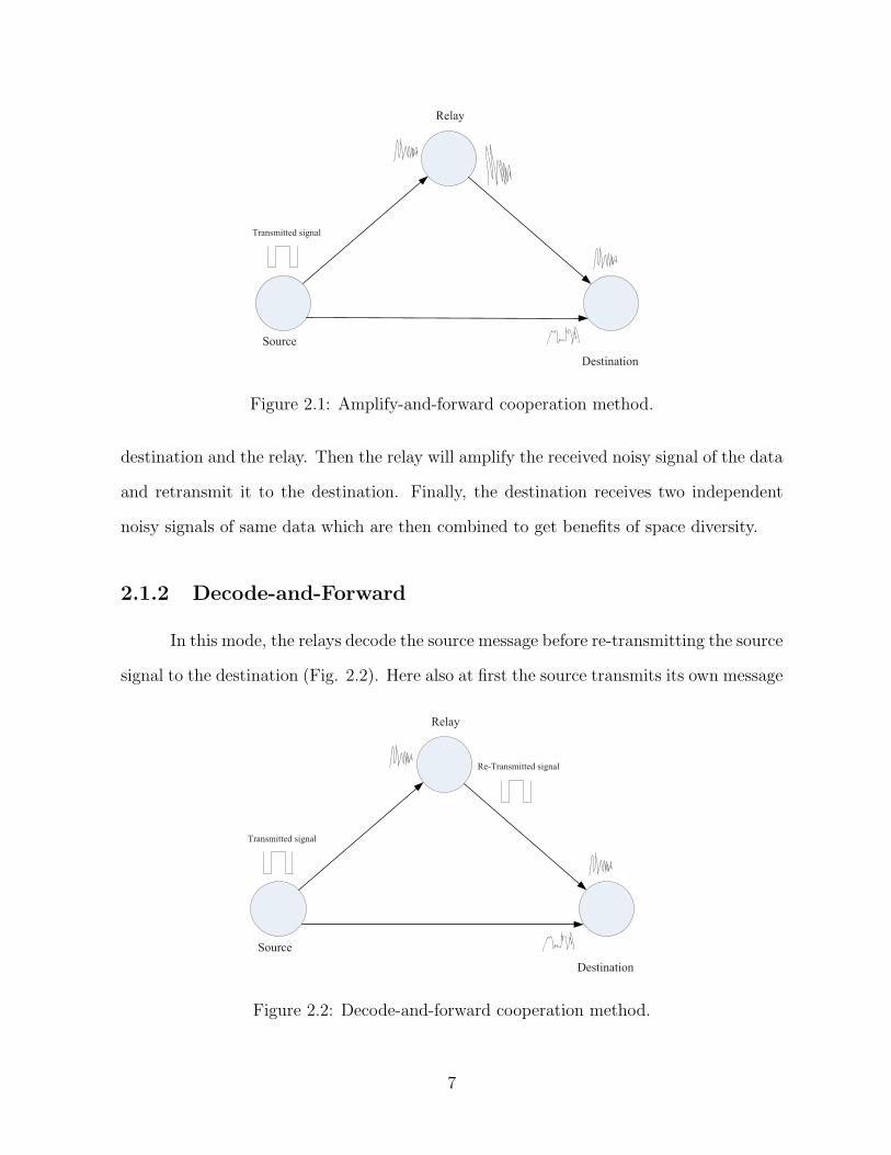
Source

Relay

Destination

Transmitted signal

Figure 2.1: Amplify-and-forward cooperation method.

destination and the relay. Then the relay will amplify the received noisy signal of the data

and retransmit it to the destination. Finally, the destination receives two independent

noisy signals of same data which are then combined to get benefits of space diversity.

2.1.2 Decode-and-Forward

In this mode, the relays decode the source message before re-transmitting the source

signal to the destination (Fig. 2.2). Here also at first the source transmits its own message

Source

Relay

Destination

Transmitted signal

Re-Transmitted signal

Figure 2.2: Decode-and-forward cooperation method.

7

to the destination and the relay. Then the relays decode the received signal from the source

and retransmit an estimate of the source data to the destination. Finally the destination

combines these signals to achieve space diversity. There are several combining techniques

that can be used to combine the same data at the destination. In the following section

we will consider several combining techniques.

2.2 Diversity Combining Techniques

In diversity techniques the destination receives same data over multiple time slots,

where each replica experiences different channel while forwarding to the destination. The

idea behind this is that, at least one of the replicas will be received correctly or at least one

link has sufficient signal-to-noise ratio (SNR) to decode the transmitted signal correctly.

Let us assume we have L replicas (L links) and the probability of error on a single link is

p, then the error probability of U independent links is pL. Therefore, the error rate of the

system decreases inversely with the Lth power of average SNR. In this case, the system

has L order diversity. In diversity combining, Selection Combining (SC), Maximal Ratio

Combining (MRC) are two common techniques. In the next subsection we will review

these two combining techniques.

2.2.1 Maximum Ratio Combining (MRC)

Let us consider a communication system when L diversity links are available at the

receiver. Then the set of received signals at the receiver can be written as

y1 =√ρh1x+ n1

y2 =√ρh2x+ n2

.

.

.

8

0 2 4 6 8 10 12 14 16 18 2010

−5

10−4

10−3

10−2

10−1

Eb/N

0, dB

Bit E

rro

r R

ate

L = 1

L = 2

L = 3

L = 4

Figure 2.3: Bit error rate of BPSK modulation with MRC in Rayleigh fading channel.

yL =√ρhLx+ nL.

where the channel gain for the Lth link is given by hL, and the independent Gaussian noise

term is denoted by nL. The average signal to noise ratio per link is ρ. The set of received

signals can be combined using MRC when channel knowledge are perfectly available at

the receiver. Therefore the received signal using MRC can be written as

y =

(

L∑

j=1

∣

∣hj

∣

∣

2

)

x+ n, (2.1)

where n is the Gaussian noise with variance per complex dimension given by(

∑L

j=1

∣

∣hj

∣

∣

2)

/2

[1]. The received effective instantaneous SNR is(

∑L

j=1

∣

∣hj

∣

∣

2)

ρ. This shows that, the SNR

of L links with MRC is the sum of each link instantaneous signal to noise ratio. Therefore

the error probability performance is decreased.

9

Figure 2.3, shows the bit error rate of binary phase shift keying (BPSK) modulation

over Rayleigh fading channel for different number of links when MRC is used at the

receiver. In this case, the fading coefcients are assumed to be known at the receiver. We

observe that the error rate performance improves with increasing the number of links.

2.2.2 Selection Combining (SC)

In selection combining, the main idea is to select the best link for a given transmis-

sion. Among the L transmissions, only the best link is selected and used for decoding. In

SC, we simply measure the received signal power for different links and make the selection

based on received signal power. This allowed us to work with one single link, i.e. the best

one at a given time. In other words, in SC the link with the highest SNR is selected

for demodulation. Therefore, the input-output relationship between the transmitted and

received signals is described in [1] as

y =

(

maxj=1,2,....L

∣

∣hj

∣

∣

)

x+ n, (2.2)

where L is number of links and n is a complex Gaussian random variable with variance

0.5 per dimension. Thus the effective instantaneous SNR after combining is given by [1]

ρSC =

(

maxj=1,2,....L

∣

∣hj

∣

∣

2)

ρ. (2.3)

Figure 2.4, shows the bit error rate of BPSK modulation over Rayleigh fading

channels for different number of links when SC is used at the receiver. In this case, the

fading coefcients are also assumed to be known at the receiver since coherent modulation

(BPSK) is used at the receiver. We observe that the error rate performance also improves

with increasing the number of links but, an interesting modulation scheme to be used in

conjunction with the SC is differential PSK (DPSK). This is because no explicit channel

estimation is needed for detection, and selection can be done using the received signal

10

0 2 4 6 8 10 12 14 16 18 2010

−5

10−4

10−3

10−2

10−1

Eb/N

0, dB

Bit E

rro

r R

ate

L=1

L=2

L=3

L=4

Figure 2.4: Bit error rate of BPSK modulation with SC in Rayleigh fading channel.

11

power, which may degrade the error performance slightly.

2.3 Jake’s Channel Model

Jake’s channel model is widely used for modeling a Rayleigh fading Channel. This

model allows an effective approximation of the desired Rayleigh fading model by using

finite number of low frequency sinusoid oscillators [14]. The complex low-pass Rayleigh

fading envelope in [15] can be written as

g (t) = gI (t) + jgQ (t) (2.4)

where

gI (t) = 2

[

M∑

n=1

cos βn cos 2πfnt+√2 cosα cos 2πfmt

]

(2.5)

gQ (t) = 2

[

M∑

n=1

sin βn cos 2πfnt+√2 sinα cos 2πfmt

]

. (2.6)

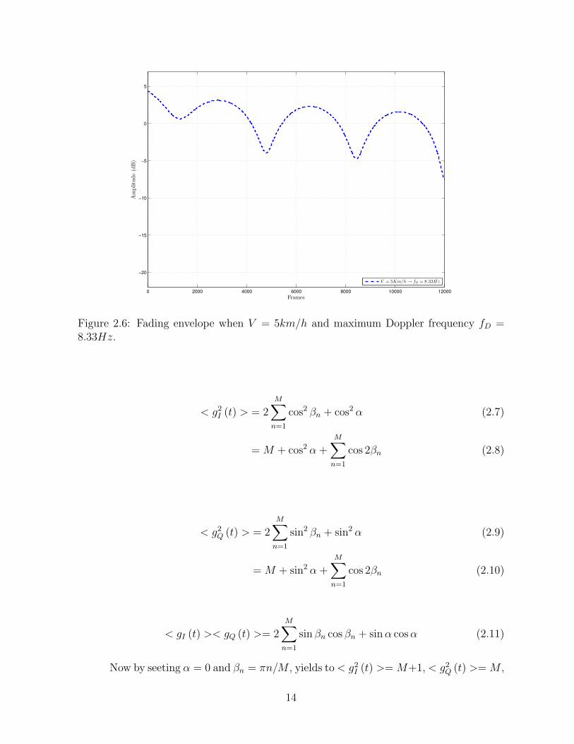
From the above, fading simulator can be constructed as shown in Fig. 2.5. Here

M is number of low frequency oscillators with frequency fn = fm cos (2πn/U) where

n = 1, 2, ....,M , and M = 4U +2. The amplitude at each frequency is set to unity except

for the frequency fm which has amplitude 1/√2.

Note that the channel phases in (2.4) are desired to be uniformly distributed. To

achieve this goal, the phases α and βn are chosen in such a way that < g2I (t) >=< g2Q (t) >

and < gI (t) gQ (t) >= 0, where < . > is a time average operator. From Fig. 2.5, < g2I (t) >

and < g2Q (t) > can be written as [15]

12

. . . . . .

. . .

Figure 2.5: Jake’s fading genarator by summing a number of low frequency oscillators,where α = 0 and βn = πn/M , gives < g2I (t) >= M + 1, < g2Q (t) >= M and <gI (t) gQ (t) >= 0 [15].

13

0 2000 4000 6000 8000 10000 12000

−20

−15

−10

−5

0

5

Frames

Amplitude(dB)

V = 5Km/h→ fD = 8.33Hz

Figure 2.6: Fading envelope when V = 5km/h and maximum Doppler frequency fD =8.33Hz.

< g2I (t) > = 2M∑

n=1

cos2 βn + cos2 α (2.7)

= M + cos2 α +M∑

n=1

cos 2βn (2.8)

< g2Q (t) > = 2M∑

n=1

sin2 βn + sin2 α (2.9)

= M + sin2 α +M∑

n=1

cos 2βn (2.10)

< gI (t) >< gQ (t) >= 2M∑

n=1

sin βn cos βn + sinα cosα (2.11)

Now by seeting α = 0 and βn = πn/M , yields to< g2I (t) >= M+1, < g2Q (t) >= M ,

14

0 2000 4000 6000 8000 10000 12000

−20

−15

−10

−5

0

5

Frames

Amplitude(dB)

V = 30Km/h → fD = 50Hz

Figure 2.7: Fading envelope when V = 30km/h and maximum Doppler frequency fD =50Hz.

0 2000 4000 6000 8000 10000 12000

−20

−15

−10

−5

0

5

Frames

Amplitude(dB)

V = 100Km/h→ fD = 167Hz

Figure 2.8: Fading envelope when V = 100km/h and maximum Doppler frequency fD =167Hz.

15

and < gI (t) gQ (t) >= 0. The mean square value < g2I > and < g2Q > can be selected

to any desired value and the Rayleigh fading envelope is obtained by using U = 34 or

M = 8 as shown in Fig. 2.6, 2.7 and 2.8 for different speeds at V = 5km/h, 30km/h and

100km/h.

2.4 Reinforcement Learning

In these algorithms the learner is a decision-making agent that takes actions in a

environment and receives reward or penalty for its actions in trying to solve a problem.

After a set of trial-and-error runs, decision maker should learn the best policy, which

is the sequence of actions that maximize the total reward (Fig. 2.9) [16]. The basic

Enviroment

Agent

RewardState Action

Figure 2.9: The agent interacts with an environment and at any state of the environmentagent takes an action that changes the state and returns a reward [16].

reinforcement learning model consists of:

• a set of states St

• a set of actions A

16

• rules of transitioning between states

• rules that determine the scalar immediate reward or penalty of a transition; and

• rules that describe what the agent observes.

In this learning process, an agent interacts with the environment in discrete time

steps. At time t, the agent receives an observation ot, which includes the reward ra.

Based on the reward, the agent chooses an action from the set of available actions which

is subsequently sent to the environment. As a result, the environment moves to a new

state st+1 and the reward rt+1. In the literature, some of the well known reinforcement

learning algorithms are: Temporal difference learning, Q-learning, State-Action-Reward-

State-Action (SARSA) [16], Learning automata [17], etc. These algorithms have been

applied successfully to problems such as robot control, elevator scheduling, telecommuni-

cations.

2.5 Q-Learning

Q-learning is a form of reinforcement learning technique. In this technique, agent

learns to find an optimal action-selection policy for any given state. Each state provides

reward to the agent for a selected action. The goal of the agent is to maximize the rewards

by selecting the best action in each state. In the next few subsections, we briefly describe

some factors that effect the Q-learning algorithm.

2.5.1 Learning Factor

The learning factor determines to what extent the recent information will override

the past information. The numerical value of learning factor is usually between 0 and 1.

17

In this case, an agent is not learning when the learning factor is 0 and learning factor

1 leads to the case where the agent considers the most recently acquired information.

Learning factor 1 is optimal for deterministic environments and learning factor is 0 when

the states are stochastic. But in practice, learning rate is assumed to be constant for all

states.

2.5.2 Discount Factor

The discount factor is responsible for the future rewards. A factor value 0 will make

the agent use the current rewards only, and a factor that approaches toward 1 will make

the agent endeavor for a long-term high reward. If the discount factor equals or greater

than 1, the action values may diverge.

2.5.3 Initial Conditions

Q-learning algorithm sets an initial condition before first update occurs, since it

is an iterative algorithm. Initial condition is set in such a way that it encourage explo-

ration. In exploration, the algorithm chooses random action and updates the Q-learning

table using the reward from the environment. Otherwise the algorithm chooses an action

associated with the highest Q-value in the Q-learning table.

2.6 Cognitive Radio

The worldwide technical advancement in mobile wireless communication and the

increasing number of mobile users, mobile devices such as cell phones, PDAs and lap-

tops have made a revolutionary change in the genus wireless communication. On the

other hand, Federal Communication Commission (FCC) measurements reveal that, cur-

rent spectrum utilization efficiency of the licensed radio spectra could be as low as 15% on

average [18]. To address this inefficiency of radio spectrum usage, the FCC has motivated

18

the use of opportunistic spectrum sharing to make the licensed frequency bands accessi-

ble for unlicensed wireless users. The main objective behind this is to create cognitive

competence of wireless devices for both licensed and unlicensed spectrum usage.

For increasing the efficiency of the spectrum usage, secondary (unlicensed) user

determines available frequency channels and respective bandwidths by using spectrum-

sensing capability. After successful sensing of opportunity, non-utilized frequency channels

are assigned to cognitive radios (CR). Simultaneous spectrum-sensing and data transmis-

sion causes degradation of Quality of service (QoS). Under this constraint two design

objectives can be considered namely, spectrum Sensing optimization and to achieve de-

sired level of QoS. To meet these design objectives, performance metric of overall system

should be maximized. Two important performance metrics in spectrum sensing should

be considered, the probability that a CR falsely detects a primary user (PU) when no PU

is present and the probability that a CR fails to detect a PU when it is present.

So far, most of the studies are focused on policy based radio, where a list of rules are

assigned for the radios to behave in a certain situation. Machine learning is a technique

that can be incorporated with CR to improve the system performance. Reinforcement

learning can be used in unknown environment, where an agent learns from trail-an-error

[19], [16]. Dynamic channel allocation using reinforcement learning has been studied

in [20]. Moreover, in [21] adaptive transmit power for spectrum management and in

[22] cooperative sensing in CR ad-hoc networks have been studied using reinforcement

learning. Efficient exploration in reinforcement learning for CR spectrum sharing has

been studied in [23]. Other learning techniques, game theory, neural networks are also

studied in the context of CR [24].

CR with multiple antennas should be chosen for more powerful spectrum sens-

ing schemes [25]. CR with multiple antenna and machine learning techniques have been

studied for environment learning in [26]. MIMO with CR utilizes simultaneous spectrum-

sensing and data transmission using multiple antenna technology to increase the through-

19

put of CR systems and avoid delay caused by spectrum sensing.

2.7 Cognitive Networks

A cognitive network can be described as a cognitive process that can realize the cur-

rent network conditions, and then plan, decide, and act on those conditions. This network

can learn from these adaptations and use them for the future decisions, by considering

end-to-end performance goals. Cognition can be used to improve the performance of re-

source management, QoS, security, access control, or many other network performance

goals compare to noncognitive networks. In most of the cases, implementing a cognitive

network requires a system that is more complex than a noncognitive network. At the same

time, cognitive network is costly in terms of overhead, architecture, and operation that

should justify the overall performance of the network [27]. In cognitive networks, goals

are based on end-to-end network performance but in the case of cognitive radio goals are

depended on only the radio user. This end-to-end performance goal helps the cognitive

network to operate in all layers of protocol stack. Another main difference is cognitive

networks are applicable both wired and wireless networks, whereas cognitive radios are

applicable only in wireless networks.

In this thesis, we propose cross-layer schemes that target cognitive networks as it

is based on learning techniques.

2.8 Conclusions

In this chapter, we have presented an overview for cooperative relay networks,

several diversity techniques, reinforcement learning, Rayleigh fading channel model, Q-

learning, cognitive radio, and cognitive networks. For the remaining chapters, we will be

using these protocols and mathematical tools to address the relays and antennas selection

issues of cooperative relay networks.

20

Chapter 3

Learning Based Relay Selection

3.1 Introduction

As an alternative of multiple antennas, cooperative diversity system allows the

receiver to see independent versions of source’s information which yield to realize the

spatial diversity without increasing the total transmit power. The two main modes of

cooperative communications are: regenerative or DF and non-regenerative or AF. In AF

mode, relay node amplifies the source message prior forwarding to the destination, whereas

in DF mode the relay decodes the source message and re-generates an estimate of this

message before forwarding to destination.

From the standpoint of DF, decoding errors occurring at relay node(s) cause severe

performance degradation in terms of symbol error rate (SER) compared to the direct

link transmission. In this case, the system suffers from detrimental effects due to error

propagation when the channel between the source and relay (S – R) is poor. In these

circumstances, relay selection is required to minimize error propagation from relay nodes

to the destination. Various methods have been proposed to reduce the error propagation

and to improve the system performance [8], [9]. For instance in [8], relay node(s) only

forward the source message if the S – R channel gain is above given threshold level. It is

21

shown in [28] that only relays with correctly decoded messages forward source message to

the destination. Other relay selection schemes where relay is selected based on maximum

SNR between relay and the destination are presented and analyzed in [10]– [11]. In [29]

the authors have shown that using media access control (MAC) layer RTS-CTS signaling,

best relay can be selected based on minimization of energy consumption.

In relay networks, selecting all reliable relay(s) is not the optimal solution for the

overall performance enhancement. Recently, many works have focused on cross-layer de-

sign approaches for relay networks. In [9], the authors presented throughput maximization

scheme based on packet and modulation size optimization, where both source and reli-

able relays realize orthogonal space time block codes (O-STBC). The work in [9] also

showed that throughput performance can be further improved through packet length and

modulation size optimization. Relay combination can also be chosen through machine

learning method, where selection is performed using past relay selection experience at the

destination.

Recently, many studies have been conducted using machine learning in cognitive

radio systems. In [30], [31] game-theoretic stochastic learning is used to address the

problem of distributed channel selection for opportunistic spectrum access. Q-learning

is another algorithm in machine learning that belongs to reinforcement learning [16],

[32]. In [33] decentralized Q-learning is used to manage aggregated interference control

in cognitive radio networks. Q-learning is also used for relay selection based on physical

layer parameters in [34]. Motivated by the works in [9], [33]– [35], we propose a cross-layer

relay selection scheme using Q-learning that maximizes the link layer throughput. Another

advantage of the proposed scheme is the average relay utilization to ensure efficient use

of the available bandwidth. In [9], all reliable relays are selected to forward the source’s

message to destination, whereas our proposed scheme always select less number of relays

compared to the scheme in [9].

The rest of the chapter is organized as follows. In section 3.2, the system model

22

is described. Derivation of transmission efficiency, the proposed relay selection algorithm

using Q-learning and simulation results are presented in section 3.3, 4.4, 3.5, respectively.

Finally conclusions are outlined in section 3.6.

3.2 System Model

We consider a cooperative diversity network consisting of a source, N relays, and

a destination as shown in Fig. 3.1. In this scheme, source node transmits a packet to the

destination node with cyclic redundancy check (CRC) bits appended to its message for

error detection. All relay nodes overhear the transmission due to the broadcast nature

of the channel. After receiving a packet, the destination and relays decode the source’s

message and check for errors. If the destination correctly decodes the source’s message,

then it sends a positive acknowledgment (ACK) to the source and relays, through a

error free feedback channel which is assumed to be perfect. Otherwise, the destination

sends negative acknowledgment (NACK) and R SEL (relay select) packet, requesting for

retransmission. When a positive ACK is received, the source transmits a new packet and

all relays remain silent. On the other hand when NACK and R SEL are received, all

selected reliable relay(s) forward source information to the destination. Fig. 3.2 and 3.3

show the time diagram and complete flow chart of the system respectively. Finally the

destination decodes the combined signal from source and relay(s) nodes.

The retransmission process continues until the destination correctly decodes the

source’s message or the number of retransmissions reaches its maximum Nmax. We assume

that the source, relays and destination are equipped with single antenna, packets are sent

through Time Division Multiple Access (TDMA) communication mode over multipath

time-varying Rayleigh fading channels modeled using Jake’s model. This model is widely

accepted for modeling the time variations of Rayleigh fading channels. We use this model

to make better decisions on relay selection using the Q-learning algorithm. This algorithm

23

S

R1

D

R2

RN

Source Destination

N Relays

hSD

Figure 3.1: Cooperative system with N relays.

S

R1

RN

DNACK

R_SEL = Relay Selection SIFS = Small Inter Frame Space

SIFS

R_SEL

.

.

.

.

.

.

Packet

ACK

TLrelays

TLrelays = Packet Transmission Time for Relays

Packet

Packet

Packet

Figure 3.2: Relay selection timing diagram

24

Source node transmits a new packet

Relay nodes check CRC. The ones

who get the right CRC become

the reliable relays. Destination

node receives and checks CRC

CRC is

correct

Destination

sends ACK

Destination

sends ACK

Destination sends NACK

Destination selects source and relay combination

from the Q-learning table to retransmit the

signal to the destination

Destination node receives and checks CRC

CRC is

correct

Yes

No

Yes

No

Yes

No

= + 1

= 0

Figure 3.3: Flow chart of the proposed system.

25

selects the best source and relay combination that maximize the transmission efficiency

by selecting either exploration or exploitation modes of operation. For simplicity, we also

assume channels are fixed for the entire duration of a packet transmission.

The complex channel coefficients of the source to destination (S-D), source to relay

(S-R) and relay to destination (R-D) links are denoted as hsd, hsr and hrd, respectively,

each modeled as complex Gaussian distributed with zero mean and unit variance. We

also denote the received signal from source to relay, source to destination and relay to

destination as ysd, ysr and yrd respectively. These received signals are given by,

ysd =√

Eshsdx+ nsd, (3.1)

ysr =√

Eshsrx+ nsr, (3.2)

yrd =√

Erhrdx+ nrd, (3.3)

where x is the transmitted source symbol and x is the estimated symbol at the relay. Es

and Er denote the transmitted energy from source and relay respectively, the noise nsd,

nsr, and nrd are additive white Gaussian each with zero mean and variance σ2. Considering

all relays, the received signal at the destination in a vector form is given by,

yrd =√

Erhrdx+Nrd, , (3.4)

In (3.4), yrd, hrd, and nrd are (N × 1) vector. These are given by,

yrd> =

[

y1 y2 ...... yN

]

, (3.5)

hrd> =

[

h1 h2 ...... hN

]

, (3.6)

Nrd> =

[

n1 n2 ...... nN

]

. (3.7)

26

In the literature, most of the studies consider perfect channel state information

(CSI) at the receiver for coherent detection. Here we use non-coherent differential Binary

Phase Shift Keying (DBPSK) to overcome the problem of channel estimation at the

receiver side and hence lower complexity. This also reduces the communication overhead

and wasted power as in pilot and training based channel estimation techniques, specially

when the fading is rapid. Non-coherent detection for cooperative communications was

studied in [36–38]. To avoid CSI estimation we employ selection combining (SC) technique

to combine the signals from source and relays. The performance of SC is inferior compared

to the maximum-ratio combining (MRC). However, the implementation of MRC requires

knowledge of instantaneous channel gain which as mentioned earlier could be impractical

in some scenarios. The conditional bit error rate (BER) for a given channel coefficient h

when DBPSK modulation is used can be written as [2],

Pb(h) =1

2exp−ρ . (3.8)

where ρ is average signal-to-noise ratio (SNR) per link.

3.3 Performance Analysis

First we define some useful parameters that will be used to evaluate the transmis-

sion efficiency (i.e. normalized throughput) of the proposed system.

• PERsd = Average Packet Error Rate (PER) of S-D link (direct transmission).

• PERretx = Average PER of retransmission.

• PERsr = Average PER of S-R link.

• SERsd = Average Symbol Error Rate (SER) of S-D link (direct transmission).

• SERRetxRelay = Average SER of retransmission.

27

• SERsr = Average SER of S-R link.

The transmission efficiency for adaptive DF is described in [9] as

η =(TL − TC)Psk

TLE(Tpacket), (3.9)

where TL and TC are the transmission time of data packet and CRC bits, respectively.

Packet successful probability of reception and average number of packet transmission per

packet are given by Ps and E(Tpacket), respectively. k is number of bits per symbol. How-

ever, in [9] the authors did not consider packet transmission time from relay to destination

indicated in Fig. 3.2. For that, the link layer transmission efficiency when considering

packet transmission time from relay to destination can be rewritten as

η =(TL − TC)Psk

TLE(Tpacket) + E(TLrelays), (3.10)

where E(TLrelays) is the average relay selection time per packet. Now,the packet successful

probability of reception Ps is given by [9],

Ps =N∑

i=0

(

1− PERsd

(

PERRetxRelay(i)Nmax

))

Pr(i), (3.11)

where N is the total number of relays, PERRetxRelay(i) denote average PER of the ith

reliable relay retransmission given by

PERRetxRelay(i) = 1− (1− SERRetxRelay(i))Lp

k (3.12)

Lp is packet length. When non of the relays could decode the source signal correctly,

which is the case when i = 0, the average PERRetxRelay(0) = 1− (1− SERRetxRelay(0))Lk

and SERRetxRelay (0) = SERsd. Pr(i) is the probability that i relays correctly decode the

28

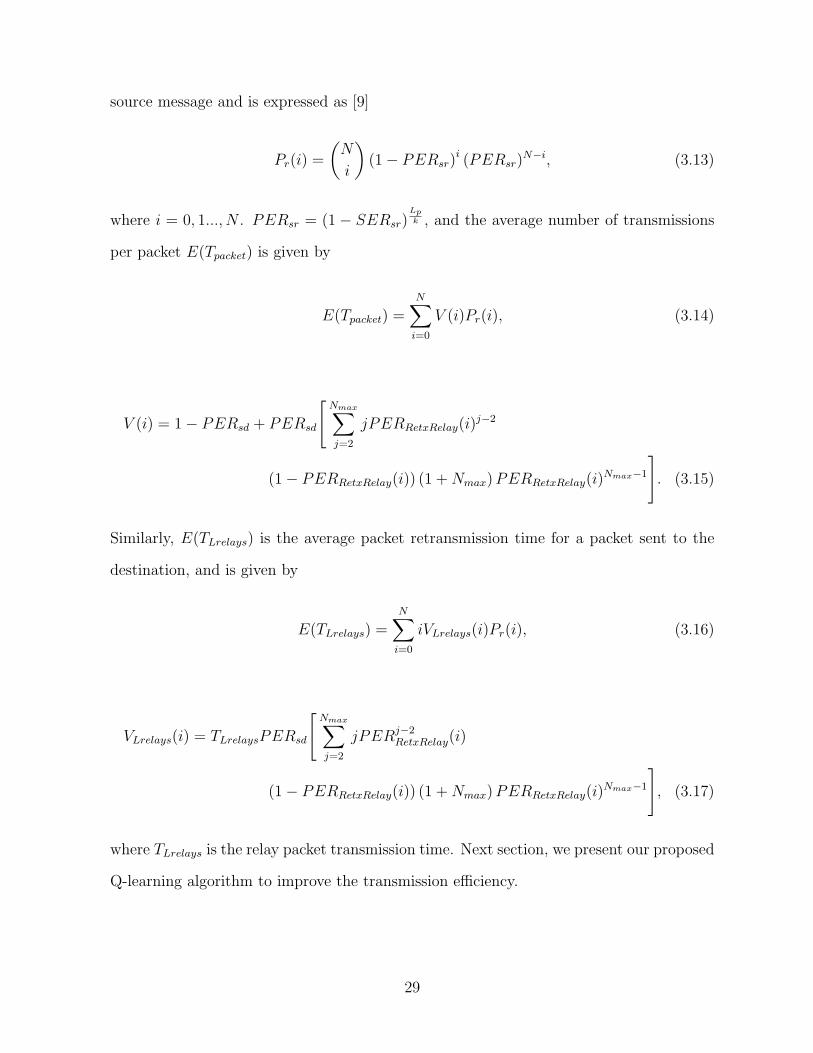
source message and is expressed as [9]

Pr(i) =

(

N

i

)

(1− PERsr)i (PERsr)

N−i, (3.13)

where i = 0, 1..., N . PERsr = (1 − SERsr)Lp

k , and the average number of transmissions

per packet E(Tpacket) is given by

E(Tpacket) =N∑

i=0

V (i)Pr(i), (3.14)

V (i) = 1− PERsd + PERsd

[

Nmax∑

j=2

jPERRetxRelay(i)j−2

(1− PERRetxRelay(i)) (1 +Nmax)PERRetxRelay(i)Nmax−1

]

. (3.15)

Similarly, E(TLrelays) is the average packet retransmission time for a packet sent to the

destination, and is given by

E(TLrelays) =N∑

i=0

iVLrelays(i)Pr(i), (3.16)

VLrelays(i) = TLrelaysPERsd

[

Nmax∑

j=2

jPERj−2RetxRelay(i)

(1− PERRetxRelay(i)) (1 +Nmax)PERRetxRelay(i)Nmax−1

]

, (3.17)

where TLrelays is the relay packet transmission time. Next section, we present our proposed

Q-learning algorithm to improve the transmission efficiency.

29

3.4 Relay Selection Using Q-learning

In the underlying system, the destination adopts Q-learning algorithm. In this

algorithm, after a set of trial-and-error, the destination should learn the best policy, which

is a sequence of actions that maximize the total reward when channels are modeled as

time-varying Rayleigh fading. For our system, an action is defined as packet transmission

process through possible source and selected reliable relay(s) combination and the reward

is defined as the transmission efficiency for a selected action. In the Q-learning algorithm,

the destination selects an action by exploration or exploitation. Here the main goal, is to

find a balance between exploration and exploitation.

In the exploration mode of the Q-learning, the destination selects a combination

where all reliable relays are present so that the destination can update all possible source

and relay combinations. It is to be noted that all relays access the channel using TDMA

mode to forward the source message to the destination. On the other hand, in the ex-

ploitation mode, the destination selects an action that has the maximum Q-value in the

Q-learning table.

The Q-table is used at the destination to store and update the Q-value for different

combinations of source and reliable relay(s). A single element subset wr is chosen from

set Wr and can be written as

Wr = {{SR1}, {SR2}, {SR3}, ....., {SR1R2...RN}}. (3.18)

For example, SR1 is defined as a single element subset of Wr when only the source(S) and

relay(R1) are used for packet transmission. Now, we define a as an action for which the

destination receives a reward ra. Reward can be calculated from (3.10) and the Q-value

Qt(a) is estimated after an action a at time t. The Q-values are updated according to

following function given by [16],

30

Table 3.1: Q-learning Table For Relay Selection

T ime Q(SR1) Q(SR2) .. Q(SRn) .. Q(SR1R2..RN )

0 0 0 .. 0 .. 0.. .. .. .. .. .. .... .. .. .. .. .. .... .. .. .. .. .. ..t1 Qt1

(SR1) Qt1(SR2) .. Qt1

(SRN ) .. Qt1(SR1R2..RN )

t1 + 1 Qt1+1(SR1) Qt1+1(SR2) .. Qt1+1(SRN ) .. Qt1+1(SR1R2..RN )

Qt+1(a) = Qt(a) + η [rt+1(a)−Qt(a)] , (3.19)

where η is the learning factor and rt+1(a) is the reward at time t+1 for action a. Qt+1(a)

is the expected value for action a at time t+ 1. Initially, we set all values of the Q-table

to zeros. After that, the destination chooses an action by exploration or exploitation. For

the selected action, the destination receives a reward (ra ≥ 0) after which it evaluates its

Q-value to update the Q-table.

Table 3.1 shows the Q-table where we can see that all Q-values are initialized to

zeros at initialization. For instance, we assume that at time t1+1 a single element subset

SRN is selected by exploitation because the Q-value of the single element subset SRN has

maximum Q-value among all elements in the Q-table at time t1. In Table 3.1, Qt1+1(SRN)

and Qt1(SRN) represent the Q-value at time t + 1 and t, respectively. At time t1 + 1,

Qt1(SRN) is updated by Qt1+1(SRN) and the remaining Q values are kept unchanged. In

this process, the destination does not need CSI information for relay selection. That is no

overhead incurred by the system where all reliable relays do not need to send extra bits

to estimate the CSI for relay selection.

3.5 Simulation Results

In this section, we present simulation results to assess the performance of the

adaptive DF cooperative system using the proposed Q-learning relay selection scheme.

31

We investigate the transmission efficiency and usage of relay combination under different

time-varying Rayleigh fading channels. The simulation parameters are as follows, packet

transmission time and CRC bits transmission time are TL = 2.667 × 10−4s and TC =

4.167 × 10−6s, respectively. It is to be noted that the packet length is set to 1024 bits,

CRC is 16 bits long and the corresponding transmission data rate is 3.84 × 106bps. The

maximum number of retransmissions per packet Nmax = 3 and unless otherwise specified,

the total number of available relays is N= 4 and the average SNR of the source to relay(s)

link is γs−r = 20dB. The channels are modeled as Rayleigh fading with fading coefficients

fixed for the entire duration of the packet transmission.

3.5.1 Q-learning Based Relay Selection Using ε Greedy Mecha-

nism

In this subsection, Q-learning algorithm selects a source and reliable relay(s) based

on ε greedy mechanism presented in [39]. In this mechanism, the destination chooses

exploration with probability ε and selects an action that has maximum Q-value in the

Q-learning table (Q-table) with probability (1−ε). The destination starts the exploration

with a very high ε value and updates ε after each successful packet transmission as in

(3.20),

ε = ε− ε

mr

. (3.20)

where mr is update parameter. From (3.20), we can write the probability of selecting a

source and relay combination as

zi =

1− ε

mr

, if the action is exploitation

ε

mr

, otherwise

(3.21)

In our simulation, we set the update parameter mr in such a way that the desti-

nation chooses exploration frequently. It is noted that exploration helps the destination

32

Algorithm 1 Q-learning algorithm for relay selection using ε greedy mechanism

1: ε = Probability of choosing exploration2: rv = Uniformly distributed [0,1]3: for (initial time to end time) do4: ε = ε/update parameter5: p = ε6: if p < rv or ε == initial value then7: Choose source and relay combination where all reliable relays are present8: else9: Choose source and relay combination associated with the highest Q-value in the

Q-table10: end if11: if ε > 1 then12: ε to initial value13: end if14: Update Q-table using (3.19)15: end for

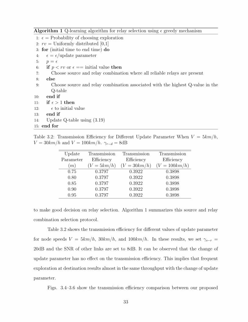
Table 3.2: Transmission Efficiency for Different Update Parameter When V = 5km/h,V = 30km/h and V = 100km/h. γr−d = 8dB

Update Transmission Transmission TransmissionParameter Efficiency Efficiency Efficiency

(m) (V = 5km/h) (V = 30km/h) (V = 100km/h)0.75 0.3797 0.3922 0.38980.80 0.3797 0.3922 0.38980.85 0.3797 0.3922 0.38980.90 0.3797 0.3922 0.38980.95 0.3797 0.3922 0.3898

to make good decision on relay selection. Algorithm 1 summarizes this source and relay

combination selection protocol.

Table 3.2 shows the transmission efficiency for different values of update parameter

for node speeds V = 5km/h, 30km/h, and 100km/h. In these results, we set γs−r =

20dB and the SNR of other links are set to 8dB. It can be observed that the change of

update parameter has no effect on the transmission efficiency. This implies that frequent

exploration at destination results almost in the same throughput with the change of update

parameter.

Figs. 3.4–3.6 show the transmission efficiency comparison between our proposed

33

0 2 4 6 8 10 12 14 16 18 200

0.1

0.2

0.3

0.4

0.5

0.6

0.7

0.8

0.9

1

Eb/N

0(dB)

Tra

nsm

issio

n E

ffic

ien

cy

Q−learning using Jakes model, V=5km/h

System in [9] using Jakes model, V=5km/h

Figure 3.4: Transmission efficiency comparison of system in [9] and Q-learning using εgreedy mechanism, under Jake’s channel model where V = 5km/h, γs−r =20dB.

system using Q-learning and ε greedy mechanism with the system in [9]. To do that, we

set the number of relays and channel gains to be identical for both schemes. It is to be

noted that the system in [9] considers all correctly decoded relays to forward the source

message to the destination. On the other hand, in our proposed system, relays are selected

based on the relay selection criteria presented in Algorithm 1. From the results, we can

see that our system provides better performance in most of the cases, which implies that

relay selection using Q-learning performed at link-layer improves the system performance.

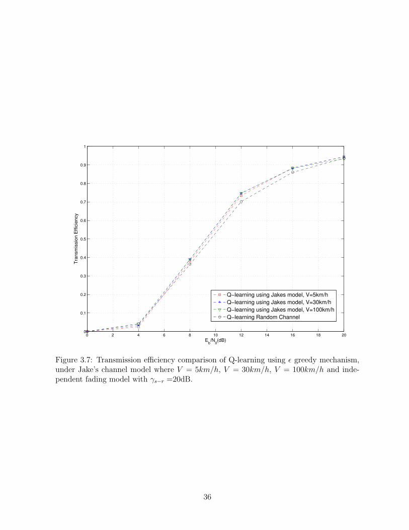
Fig. 3.7 also shows the transmission efficiency comparison between Q-learning

based ε greedy mechanism under Jake’s Rayleigh fading model with V = 5km/h, 30km/h,

and 100km/h and the case of independent fading realizations. From the results, we can see

that both cases perform almost identical from low SNRs to high SNRs, because Algorithm

1 operates in such a way that the destination chooses exploration more than exploitation.

Note that, in the independent channel model case, the probability of selecting incorrect

34

0 2 4 6 8 10 12 14 16 18 200

0.1

0.2

0.3

0.4

0.5

0.6

0.7

0.8

0.9

1

Eb/N

0(dB)

Tra

nsm

issio

n E

ffic

ien

cy

Q−learning, using jakes model, V=30km/h

System in [9], using jakes model V=30km/h

Figure 3.5: Transmission efficiency comparison of system in [9] and Q-learning using εgreedy mechanism, under Jake’s channel model is used where V = 30km/h, γs−r =20dB.

0 2 4 6 8 10 12 14 16 18 200

0.1

0.2

0.3

0.4

0.5

0.6

0.7

0.8

0.9

1

Eb/N

0(dB)

Tra

nsm

issio

n E

ffic

iency


System in [9] using Jakes model V=100km/h

Figure 3.6: Transmission efficiency comparison of system in [9] and Q-learning using εgreedy mechanism, under Jake’s channel model is used where V = 100km/h, γs−r =20dB.

35

0 2 4 6 8 10 12 14 16 18 200

0.1

0.2

0.3

0.4

0.5

0.6

0.7

0.8

0.9

1

Eb/N

0(dB)

Tra

nsm

issio

n E

ffic

ien

cy




Q−learning Random Channel

Figure 3.7: Transmission efficiency comparison of Q-learning using ε greedy mechanism,under Jake’s channel model where V = 5km/h, V = 30km/h, V = 100km/h and inde-pendent fading model with γs−r =20dB.

36

0 2 4 6 8 10 12 14 16 18 200

0.1

0.2

0.3

0.4

0.5

0.6

0.7

0.8

0.9

1

Eb/N0(dB)

Tra

nsm

issio

n E

ffic

iency

Q−learning, using jakes model, V=5km/h and N = 8

Q−learning, using jakes model, V=5km/h and N = 12

Q−learning, Random Channel and N = 8

Q−learning, Random Channel and N = 12

Figure 3.8: Transmission efficiency comparison of Q-learning using ε greedy mechanism,under Jake’s channel model where V = 5km/h and independent fading model withγs−r =20dB, N = 8 and 12.

relay combination is small when the number of relays is also small. Another reason is

that the Q-learning using ε greedy mechanism algorithm is suitable since it learns how

many relays are good for maximizing the link layer transmission efficiency. From here we

can say that if we have small number of relays in the network, the probability of selecting

incorrect relay combination is also small for Q-learning using independent channel model.

Fig. 3.8 shows the throughput performance using Jake’s fading model compared

with the independent channel case using Q-learning based ε greedy mechanism when a

network has larger number of relays. In both cases, it is observed that our proposed selec-

tion performs well when the time variation in the fading model are utilized. This implies

that when a network has larger number of relays, the probability of selecting a incorrect

relay combination is higher for the system under independent channel realizations. On the

other-hand, the Q-learning algorithm utilizes the memory introduced in the time-varying

channel to learn about the channel and using learning process the destination takes proper

37

1 2 3 4 5 6 7 80.32

0.34

0.36

0.38

0.4

0.42

0.44

0.46

Number of Relays

Tra

nsm

issio

n E

ffic

iency

Figure 3.9: Transmission efficiency vs number of relays where Q-learning using ε greedymechanism is used, and Jake’s channel model is also used where V = 5km/h.γs−r =20dBand γr−d =8dB

decision based on previous relay selection experience.

Fig. 3.9 shows the throughput performance as a function of number of relays in the

network. These results are based on fixed SNR from relays to the destination. However,

from the source to relay the SNR is fixed to 20dB. Results show that as we increase the

number of relays in the network, the throughput performance is improved. This is due to

the fact that, the large number of relays in the network allows more links from the relay

nodes to the destination. As a result, once the exploration is completed, the destination

has a large number of combination to find the proper combination from the Q-learning

table to maximize the throughput.

38

Algorithm 2 Effect of exploration to exploitation ratio on Q-learning relay selectionalgorithm

1: integer = xn

2: for (initial time to end time) do3: if counter == 0 or first packet then4: Choose source and relay combination where all reliable relays are present5: else6: Choose source and relay combination associated with the highest Q-value in the

Q-table7: counter = counter + 18: end if9: if counter ≥ xn then10: counter = 011: end if12: Update Q-table using (3.19)13: end for

3.5.2 Effect of Exploration to Exploitation Ratio (EER) on Q-

learning Relay Selection

In this subsection, our algorithm operates in such a way that the destination chooses

the exploitation mode more than the exploration mode where the destination adopts

the Q-learning algorithm for relay combination selection. In this case, the destination

operates in the exploration mode after certain fixed number of packets. Otherwise, the

destination operates in the exploitation mode for relay combination selection using the

Q-learning table. In our simulations, we noted that the exploration mode helps the

destination to make proper decisions on future relay selection. However, operating in the

exploration mode is known to be expensive since in this case all reliable relays participate

in retransmissions as our system employs TDMA for relay communications. Algorithm 2

summarizes this source and relay combination selection protocol.

Tables 3.3–3.5 show the transmission efficiency for different exploration to exploita-

tion ratios when V = 5km/h, 30km/h, and 100km/h. We set the SNR from source to

relay link γs−r = 20dB and all other links are set at 8dB. From the results, we can see that

for all three cases, the transmission efficiency changes with the change of exploration to

39

Table 3.3: Transmission efficiency for different exploration to exploitation ratio. V =5km/h. γr−d = 8dB

Exploration to Transmission EfficiencyExploitation ratio (V = 5km/h)

1/100 0.36001/1000 0.36321/2000 0.37561/3000 0.38981/4000 0.39431/5000 0.40771/6000 0.45491/7000 0.46521/7100 0.49071/7200 0.44211/7900 0.38771/8000 0.3607



1/100 0.36121/1000 0.38041/2000 0.39791/3000 0.42971/4000 0.42601/5000 0.44241/6000 0.45491/7000 0.49521/7100 0.50091/7200 0.48901/8000 0.47261/8500 0.3986

40



1/100 0.39641/1000 0.46291/2000 0.48051/3000 0.49981/4000 0.46681/5000 0.46591/6000 0.45471/7000 0.3759

exploitation ratio (EER). It can be noted that, EER 1/7100 provides the maximum trans-

mission efficiency for both cases, when V = 5km/h and V = 30km/h. Similarly, when

V = 100km/h EER 1/3000 provides maximum transmission efficiency. It can also be

noted that for V = 100km/h exploration to exploitation ratio increased because channel

changes very fast compared to other two cases when V = 5km/h and 30km/h.

Figs. 3.10–3.12 show the transmission efficiency comparison between the system

in [9], the effect of exploration-to-exploitation ratio on the Q-learning and the effect of ε

greedy mechanism on Q-learning. From the results, one can see that in all three cases, the

EER outperforms the Q-learning using ε greedy mechanism and the system in [9]. This

implies that exploration is more expensive than exploitation in TDMA communication

mode, as in exploration all reliable relays participate to forward the source information

to the destination.

Fig. 3.13 shows the effect of exploration-to-exploitation ratio on the Q-learning

relay selection algorithm when the channels are modeled using Jake’s Rayleigh fading

model with V = 5km/h, 30km/h, and 100km/h and the case of independent fading

realizations. As the results show, our Q-learning algorithm utilizes the memory introduced

in the time-varying channel to learn about the different channels, and uses this learning

process to improve the relay selection procedure as time elapses.

41

0 2 4 6 8 10 12 14 16 18 200

0.1

0.2

0.3

0.4

0.5

0.6

0.7

0.8

0.9

1

Eb/N

0(dB)

Tra

nsm

issio

n E

ffic

iency

Q−learning using ε greedy mechanism

Q−learning exploration−to−exploitation ratio (EER)

System in [9]

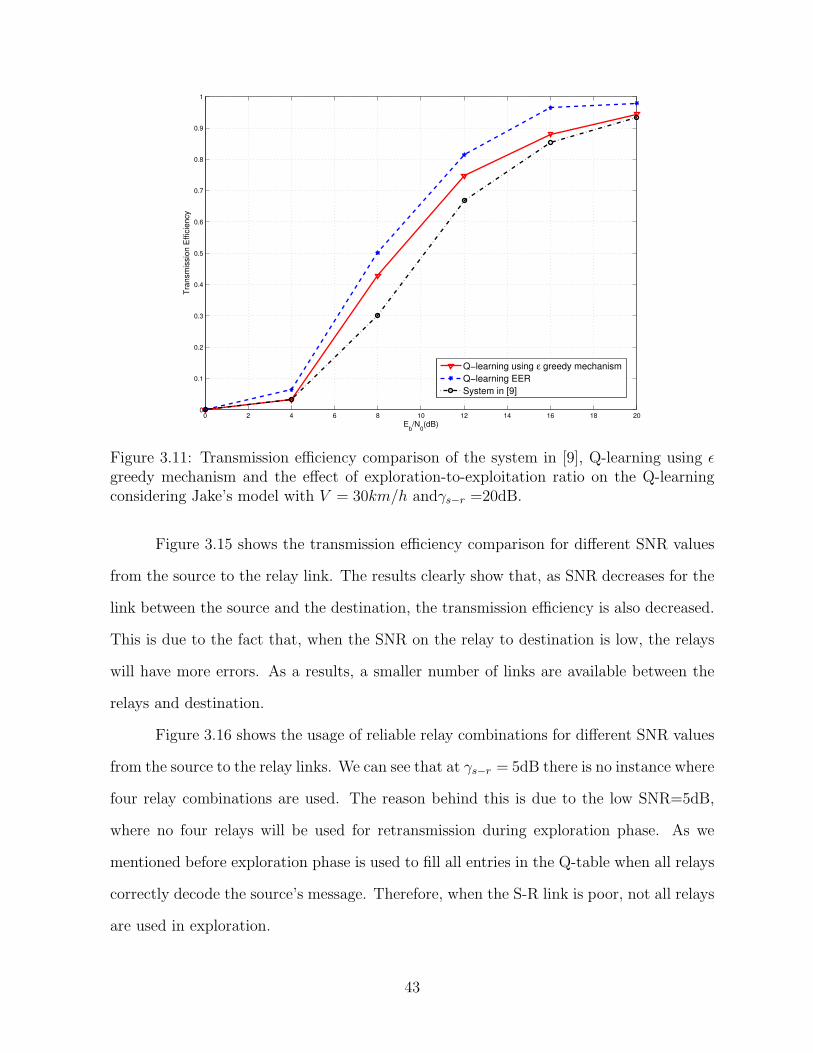
Figure 3.10: Transmission efficiency comparison of the system in [9], Q-learning using εgreedy mechanism and the effect of exploration-to-exploitation ratio on the Q-learningconsidering Jake’s model with V = 5km/h andγs−r =20dB.

Fig. 3.14 shows the percentage usage of relay combination for the system in [9]

and the effect of the exploration-to-exploitation ratio on the Q-learning algorithm. As

evident from these results, the percentage of relay usage for the system [9] is always four

regardless of the link quality given by the SNRs. This is expected as the system in [9]

is based on fixed number of relays. However, the number of transmitting relays varies

for our Q-learning based cross-layer approach as it maximizes the link-layer transmission

efficiency. In other-wards, Fig. 3.14 indicates the percentages of usage of relays that

maximizes the transmission efficiency. From the results, one can see that at low SNRs,

small number of relays are employed as the channels between relays to the destination

are poor. As the SNR increases, channels become more reliable and more relays are used

in retransmission. Also one should note that as the node speed goes high, the Q-learning

acts on the limited memory of the channel and hence, more relays are employed relative

to the case with lower node speeds.

42

0 2 4 6 8 10 12 14 16 18 200

0.1

0.2

0.3

0.4

0.5

0.6

0.7

0.8

0.9

1

Eb/N

0(dB)

Tra

nsm

issio

n E

ffic

iency

Q−learning using ε greedy mechanism

Q−learning EER

System in [9]


Figure 3.15 shows the transmission efficiency comparison for different SNR values

from the source to the relay link. The results clearly show that, as SNR decreases for the

link between the source and the destination, the transmission efficiency is also decreased.

This is due to the fact that, when the SNR on the relay to destination is low, the relays

will have more errors. As a results, a smaller number of links are available between the

relays and destination.

Figure 3.16 shows the usage of reliable relay combinations for different SNR values

from the source to the relay links. We can see that at γs−r = 5dB there is no instance where

four relay combinations are used. The reason behind this is due to the low SNR=5dB,

where no four relays will be used for retransmission during exploration phase. As we

mentioned before exploration phase is used to fill all entries in the Q-table when all relays

correctly decode the source’s message. Therefore, when the S-R link is poor, not all relays

are used in exploration.

43

0 2 4 6 8 10 12 14 16 18 200

0.1

0.2

0.3

0.4

0.5

0.6

0.7

0.8

0.9

1

Eb/N

0(dB)

Tra

nsm

issio

n E

ffic

iency

Q−learning, using ε greedy mechanism

Q−learning, EER

System in [9]


0 2 4 6 8 10 12 14 16 18 200

0.1

0.2

0.3

0.4

0.5

0.6

0.7

0.8

0.9

1

Eb/N

0(dB)

Tra

nsm

issio

n E

ffic

iency

Q−learning, EER, V=5km/h



Q−learning, EER, Random Channel

Figure 3.13: Effect of exploration-to-exploitation ratio with node speed V = 5km/h,V = 30km/h, V = 100km/h and independent fading model with γs−r =20dB.

44

0 4 8 12 16 200

50

100

0 4 8 12 16 200

50

100

0 4 8 12 16 200

50

100

0 4 8 12 16 200

50

100

Perc

enta

ge u

sage o

f re

lay c

om

bin

ation (

%)

0 4 8 12 16 200

50

100

Eb/N

0 (dB)

1 Relay 2 Relays 3 Relays 4 Relays

V = 5 km/h

V = 100 km/h

V = 30 km/h

Random

All realys

Figure 3.14: Usage of reliable relay combination for system in [9], effect of exploration toexploitation ratio on Q-learning when channels are Jake’s Rayleigh fading channel withV = 5km/h, V = 30km/h, V = 100km/h and effect of exploration to exploitation ratioon Q-learning when channels are random.γs−r = 20dB.

45

0 2 4 6 8 10 12 14 16 18 200

0.1

0.2

0.3

0.4

0.5

0.6

0.7

0.8

0.9

1

Eb/N

0(dB)

Tra

nsm

issio

n E

ffic

iency

Q−learning, S−R = 20dB



Figure 3.15: Transmission efficiency comparison for different SNR values of S-R link.Where, jake’s model is used as fading channel, V = 5km/h.

0 4 8 12 16 200

50

100

0 4 8 12 16 200

20

40

60

80

100

0 4 8 12 16 200

20

40

60

80

100

Pe

rce

nta

ge

usa

ge

of

rela

y c

om

bin

atio

n (

%)

Eb/N

0 (dB)

1 Relay 2 Relays 3 Relays 4 Relays

γs−r

= 20dB

γs−r

= 10dB

γs−r

= 5dB

Figure 3.16: Usage of reliable relay combination for different SNR values of S-R link.Where, Jake’s model is used as fading channel, V = 5km/h.

46

3.6 Conclusions

In this chapter, we have presented Q-learning based cross-layer relay selection

scheme to maximize the link layer transmission efficiency. The proposed learning al-

gorithm utilizes the memory introduced by the time-varying Rayleigh fading channel to

learn and act on future relay selections. Hence improved throughput maximization rela-

tive to the conventional schemes with no learning involved. We have examined that the

ε greedy mechanism and the effect of exploration-to-exploitation ratio on the Q-learning

provide transmission efficiency gain over existing systems where all reliable relays partici-

pate in retransmission. Moreover, our proposed system utilizes the channel resources more

efficiently than existing systems. Hence the system uses the bandwidth more efficiently

and also provides improved transmission efficiency.

47

Chapter 4

Learning Based Transmit Antenna

Selection of Multiple-Antenna Relays

In the previous chapter, we have considered all relays operating with a single trans-

mit antenna and determined the transmission efficiency. To meet the increasing demand

for high data rate services, transmit antenna diversity has been widely embraced as ef-

fective method to enhance the capacity of wireless systems, while operating on the same

bandwidth compared to the single antenna case. In this chapter, we extend our study of

chapter 3 to design relay networks with multiple antennas over Rayleigh fading channels.

4.1 Introduction

MIMO technology can potentially improve network throughput and transmission

reliability by utilizing multiple antennas at the transmitter and/or at the receiver. Now

it has been widely used in many standards [40]–[42] due to its ability to significant per-

formance enhancement of wireless communication systems [43], [44]. In this technology,

multiplexing techniques take advantage of the rich scattering environment to increase

transmission capacity [45] and diversity combats fading to enhance the transmission reli-

ability [46], [47].

48

In the previous chapter, all relays in the system are assumed to be equipped with

a single antenna. This precludes the beneficial use of MIMO technology in conjunction

with relaying systems. However, it has been theoretically shown that the performance of

relaying systems can be significantly enhanced by exploiting the benefits offered by MIMO

technology [48]. In [48] the author investigated ergodic capacity of dual-hop AF MIMO

system. The work in [49] shows the effect of multiple antennas on outage probability in

relay networks.

In multiple antenna environment, selecting all antennas is not an optimal solution

as cost increases with the number of RF chains needed for multiple antennas. A MIMO

system with antenna selection can improve the performance compared to the case with

no antenna selection. However, the computational load and extra memory are required

for an optimal selection through an exhaustive search over all possible antenna subsets

[50], [51]. This load grows exponentially with the increase of total number of available

antennas. To address this issue, antennas can be selected by machine learning techniques

using past antenna selection experience. In [52], machine learning is used for channel

selection in cognitive ad-hoc Single-Input and Single-Output (SISO) networks. Machine

learning is also used in [53] to address the channel allocation problem for heterogenous

cognitive networks. Similar to previous chapter, the Q-learning algorithm can also be

implemented in antenna selection for the relay nodes. In [54], co-operative Q-learning

is used to assign channels for cognitive nodes. Q-learning is also used in [55] to assign

channels for two cognitive nodes from a set of two channels. On the other hand, in [56] the

authors evaluated the performance of user satisfaction based Q-learning channel selection

algorithm for ad-hoc networks where cognitive nodes in heterogeneous environments are

considered.

Motivated by the works in [9], [49], [50], [51], we propose a cross-layer antenna

selection scheme from the reliable relays using Q-learning that maximize the link layer

throughput. Another advantage of the proposed scheme is due to the average antenna

49

utilization of reliable relays to ensure efficient use of available bandwidth. From the above,

this chapter is organized as follows. Section 4.2, describes the system model for multiple-

antennas relay networks. Performance analysis is presented in section 4.3. Simulation

settings and results of the proposed algorithm are presented in Section 4.5. Finally,

conclusions are drawn in Section 4.6.

4.2 System Model

Similar to chapter 3, here we also consider a cooperative diversity network con-

sisting of a source, a destination and N relays as shown in Fig. 4.1. In this scheme,

source node transmits a packet to the destination node with cyclic redundancy check

(CRC) bits appended to its message for error detection. All relay nodes overhear the

transmission due to the broadcast nature of the channel. After receiving a packet, the

destination and relays decode the source’s message and check for errors. If the destination

correctly decodes the source’s message, then it sends a positive acknowledgment (ACK)

to the source and relays, through a error free feedback channel which is assumed to be

perfect. Otherwise, the destination sends negative acknowledgment (NACK) and A SEL

(antenna select) packet, requesting for retransmission. When a positive ACK packet is

received, the source transmits a new packet and all relays remain silent. But when NACK

and A SEL are received, all selected antenna associated with reliable relay(s) forward

source information to the destination. Figs. 3.2 and 3.3 show the time diagram and the

complete flow chart of the system. Finally the destination decodes the combined signal

from source and relay(s) nodes.

This retransmission process continues until the destination correctly decodes the

source’s message or the number of retransmission reaches its maximum Nmax. We assume

source and destination are equipped with single antenna. But the relays are equipped

with one receive antenna and NT transmit antennas. All packets are sent through TDMA

50

TX1

TXN

.

.

.

TX1

TXN

.

.

.

TX1

TXN

.

.

.

.

.

.

.

.

Relay 1

Relay 2

Relay N

Source Destination

RX

RX

RX

TX RX

Figure 4.1: Schematic illustration of the system under consideration.

51

Source node transmits a new packet

Relay nodes check CRC. The ones

who get the right CRC become

the reliable relays. Destination

node receives and checks CRC

CRC is

correct

Destination

sends ACK

Destination

sends ACK

Destination sends NACK

Destination selects source and relay’s antenna

combination from the Q-learning table to retransmit

the

signal to the destination

Destination node receives and checks CRC

CRC is

correct

Yes

No

Yes

No

Yes

No

= + 1

= 0

Figure 4.2: Flow chart of the proposed system.

52

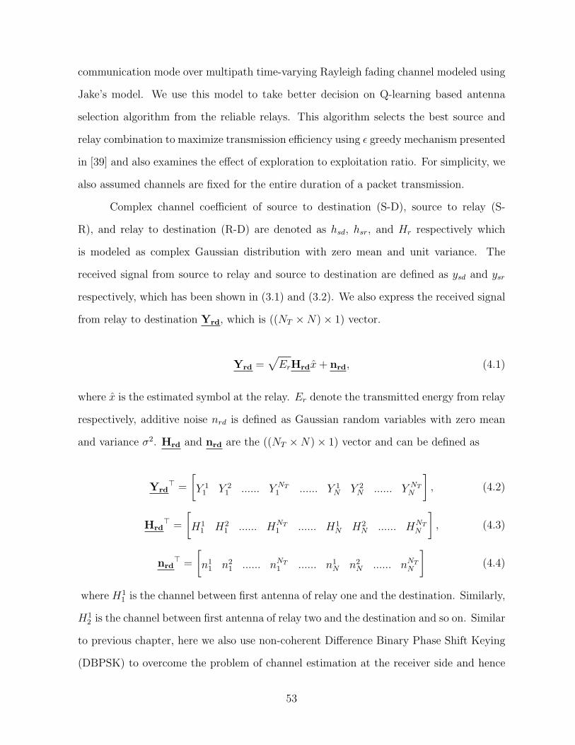
communication mode over multipath time-varying Rayleigh fading channel modeled using

Jake’s model. We use this model to take better decision on Q-learning based antenna

selection algorithm from the reliable relays. This algorithm selects the best source and

relay combination to maximize transmission efficiency using ε greedy mechanism presented

in [39] and also examines the effect of exploration to exploitation ratio. For simplicity, we

also assumed channels are fixed for the entire duration of a packet transmission.

Complex channel coefficient of source to destination (S-D), source to relay (S-

R), and relay to destination (R-D) are denoted as hsd, hsr, and Hr respectively which

is modeled as complex Gaussian distribution with zero mean and unit variance. The

received signal from source to relay and source to destination are defined as ysd and ysr

respectively, which has been shown in (3.1) and (3.2). We also express the received signal

from relay to destination Yrd, which is ((NT ×N)× 1) vector.

Yrd =√

ErHrdx+ nrd, (4.1)

where x is the estimated symbol at the relay. Er denote the transmitted energy from relay

respectively, additive noise nrd is defined as Gaussian random variables with zero mean

and variance σ2. Hrd and nrd are the ((NT ×N)× 1) vector and can be defined as

Yrd> =

[

Y 11 Y 2

1 ...... Y NT

1 ...... Y 1N Y 2

N ...... Y NT

N

]

, (4.2)

Hrd> =

[

H11 H2

1 ...... HNT

1 ...... H1N H2

N ...... HNT

N

]

, (4.3)

nrd> =

[

n11 n2

1 ...... nNT

1 ...... n1N n2

N ...... nNT

N

]

(4.4)

where H11 is the channel between first antenna of relay one and the destination. Similarly,

H12 is the channel between first antenna of relay two and the destination and so on. Similar

to previous chapter, here we also use non-coherent Difference Binary Phase Shift Keying

(DBPSK) to overcome the problem of channel estimation at the receiver side and hence

53

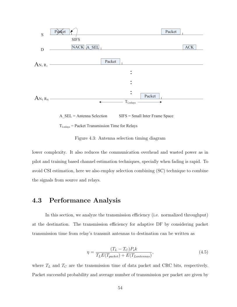
S

AN1 R1

ANT RN

DNACK

A_SEL = Antenna Selection SIFS = Small Inter Frame Space

SIFS

A_SEL

.

.

.

.

.

.

Packet

ACK

TLrelays

TLrelays = Packet Transmission Time for Relays

Packet

Packet

Packet

Figure 4.3: Antenna selection timing diagram

lower complexity. It also reduces the communication overhead and wasted power as in

pilot and training based channel estimation techniques, specially when fading is rapid. To

avoid CSI estimation, here we also employ selection combining (SC) technique to combine

the signals from source and relays.

4.3 Performance Analysis

In this section, we analyze the transmission efficiency (i.e. normalized throughput)

at the destination. The transmission efficiency for adaptive DF by considering packet

transmission time from relay’s transmit antennas to destination can be written as

η =(TL − TC)Psk

TLE(Tpacket) + E(TLantennas), (4.5)

where TL and TC are the transmission time of data packet and CRC bits, respectively.

Packet successful probability and average number of transmission per packet are given by

54

Ps and E(Tpacket), respectively. k is number of bits per symbol and E(TLantennas) is the

average packet transmission time from the relay’s antennas to the destination per packet.

Now, the packet successful probability Ps is given by [9],

Ps =N∑

i=0

(

1− PERsd (PERRetxAntenna(i))Nmax

)

Pr(i), (4.6)

where N is the total number of relays, PERRetxAntenna(i) denote the average PER of the

ith reliable relay retransmission given by

PERRetxAntenna(i) = 1− (1− SERRetxAntenna(i))Lp

k (4.7)

SERRetxAntenna is average SER of retransmission and Lp is total packet length. When

not a single relay could decode the source signal correctly, which is the case when i = 0,

the average PERRetxAntenna(0) = 1− (1− SERRetxAntenna(0))Lk and SERRetxAntenna (0) =

SERsd. Pr(i) is the probability that i relays correctly decode the source message has been

shown in (3.13)

The average number of transmission time per packet E(Tpacket) and is given by

E(Tpacket) =N∑

i=0

Vpacket(i)Pr(i), (4.8)

Vpacket(i) = 1− PERsd + PERsd

[

Nmax∑

j=2

j(PERRetxAntenna(i))j−2

(1− PERRetxAntenna(i)) (1 +Nmax) (PERRetxAntenna(i))Nmax−1

]

. (4.9)

Similarly, E(TLantennas) is the average packet retransmission time for a packet sent the

55

destination, and is given by

E(TLantennas) = NT

N∑

i=0

iVLantennas(i)Pr(i), (4.10)

VLantennas(i) = TLantennasPERsd

[

Nmax∑

j=2

j(PERRetxAntenna(i))j−2

(1− PERRetxAntenna(i)) (1 +Nmax) (PERRetxAntenna(i))Nmax−1

]

. (4.11)

where NT is number of transmit antennas per relay and TLantennas is the packet trans-

mission time from an antenna. In next subsection, we present our proposed Q-learning

algorithm to select transmit antenna from the reliable relays to improve the transmission

efficiency.

4.4 Transmit Antenna Selection Using Q-learning

Similar to previous chapter, the destination also adopts Q-learning algorithm. In

this algorithm, the destination should learn to choose the best action after a set of trail and

error to maximize the total reward when channels are modeled as time-varying Rayleigh

fading. For our system, an action is defined as packet transmission process through

possible source and selected reliable relay’s transmit antenna(s) combination and the

reward is defined as the transmission efficiency for a selected action. In the Q-learning

algorithm, destination selects an action by exploration or exploitation. Here the main

goal is also finding a balance between exploration and exploitation.

In exploration mode of the Q-learning, the destination selects a combination where

all reliable relay’s transmit antenna are present so that destination can update all pos-

sible source and relay’s transmit antenna combinations. It can be noted that, all relay’s

transmit antenna access the channel using the channel using TDMA mode to forward the

56

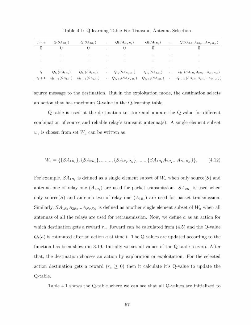
Table 4.1: Q-learning Table For Transmit Antenna Selection

T ime Q(SA1R1) Q(SA2R1

) .. Q(SANT R1) Q(SA1R2

) .. Q(SA1R1A2R2

...ANT RN)

0 0 0 .. 0 0 .. 0.. .. .. .. .. .. .. .... .. .. .. .. .. .. .... .. .. .. .. .. .. ..t1 Qt1

(SA1R1) Qt1

(SA2R1) .. Qt1

(SANT R1) Qt1

(SA1R2) .. Qt1

(SA1R1A2R2

...ANT RN)

t1 + 1 Qt1+1(SA1R1) Qt1+1(SA2R1

) .. Qt1+1(SANT R1) Qt1+1(SA1R2

) .. Qt1+1(SA1R1A2R2

...ANT RN)

source message to the destination. But in the exploitation mode, the destination selects

an action that has maximum Q-value in the Q-learning table.

Q-table is used at the destination to store and update the Q-value for different

combination of source and reliable relay’s transmit antenna(s). A single element subset

wa is chosen from set Wa can be written as

Wa = {{SA1R1}, {SA2R1

}, ........, {SANTRN}, ....., {SA1R1

A2R2...ANTRN

}}, (4.12)

For example, SA1R1is defined as a single element subset of Wa when only source(S) and

antenna one of relay one (A1R1) are used for packet transmission. SA2R1

is used when

only source(S) and antenna two of relay one (A1R1) are used for packet transmission.

Similarly, SA1R1A2R2

...ANTRNis defined as another single element subset of Wa when all

antennas of all the relays are used for retransmission. Now, we define a as an action for

which destination gets a reward ra. Reward can be calculated from (4.5) and the Q-value

Qt(a) is estimated after an action a at time t. The Q-values are updated according to the

function has been shown in 3.19. Initially we set all values of the Q-table to zero. After

that, the destination chooses an action by exploration or exploitation. For the selected

action destination gets a reward (ra ≥ 0) then it calculate it’s Q-value to update the

Q-table.

Table 4.1 shows the Q-table where we can see that all Q-values are initialized to

57

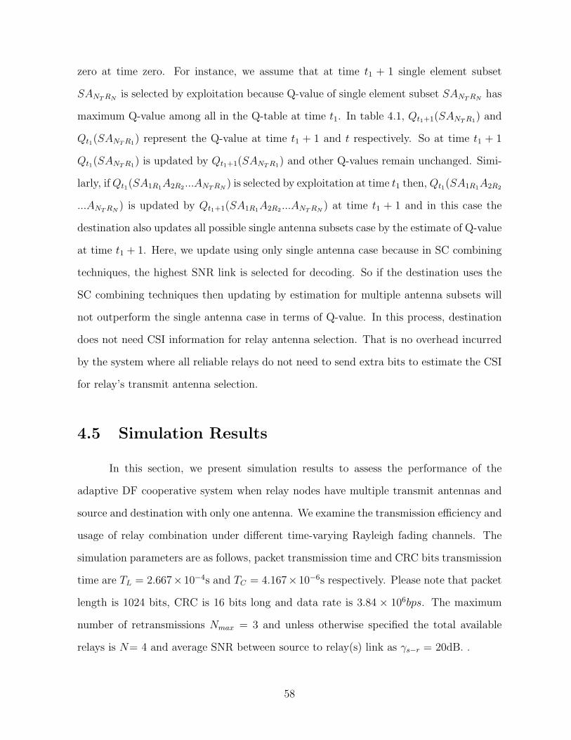
zero at time zero. For instance, we assume that at time t1 + 1 single element subset

SANTRNis selected by exploitation because Q-value of single element subset SANTRN

has

maximum Q-value among all in the Q-table at time t1. In table 4.1, Qt1+1(SANTR1) and

Qt1(SANTR1) represent the Q-value at time t1 + 1 and t respectively. So at time t1 + 1

Qt1(SANTR1) is updated by Qt1+1(SANTR1

) and other Q-values remain unchanged. Simi-

larly, ifQt1(SA1R1A2R2

...ANTRN) is selected by exploitation at time t1 then, Qt1(SA1R1

A2R2

...ANTRN) is updated by Qt1+1(SA1R1

A2R2...ANTRN

) at time t1 + 1 and in this case the

destination also updates all possible single antenna subsets case by the estimate of Q-value

at time t1 + 1. Here, we update using only single antenna case because in SC combining

techniques, the highest SNR link is selected for decoding. So if the destination uses the

SC combining techniques then updating by estimation for multiple antenna subsets will

not outperform the single antenna case in terms of Q-value. In this process, destination

does not need CSI information for relay antenna selection. That is no overhead incurred

by the system where all reliable relays do not need to send extra bits to estimate the CSI

for relay’s transmit antenna selection.

4.5 Simulation Results

In this section, we present simulation results to assess the performance of the

adaptive DF cooperative system when relay nodes have multiple transmit antennas and

source and destination with only one antenna. We examine the transmission efficiency and

usage of relay combination under different time-varying Rayleigh fading channels. The

simulation parameters are as follows, packet transmission time and CRC bits transmission

time are TL = 2.667× 10−4s and TC = 4.167× 10−6s respectively. Please note that packet

length is 1024 bits, CRC is 16 bits long and data rate is 3.84 × 106bps. The maximum

number of retransmissions Nmax = 3 and unless otherwise specified the total available

relays is N= 4 and average SNR between source to relay(s) link as γs−r = 20dB. .

58

4.5.1 Q-learning Based Antenna Selection Using ε Greedy Mech-

anism

In this subsection, Q-learning algorithm selects a source and antenna(s) combi-

nation from the reliable relays based on ε greedy mechanism presented in [39]. In this

mechanism, the destination chooses exploration with probability ε and selects an action

that has maximum Q-value in Q-learning table (Q-table) with probability (1 − ε). The

Destination starts the exploration with a very high ε value and updates ε after each

successful packet transmission as in (4.13),

ε = ε− ε

ma

. (4.13)

where ma is the update parameter. From (4.13), we can write the probability of selecting

a source and antenna(s) combination as

zj =

1− ε

ma

, if the action is exploitation

ε

ma

, otherwise

(4.14)

In our simulation, we set the update parameter mr in such a way that the des-

tination chooses exploration frequently. It is to be noted that, exploration helps the

destination to make good decision on antenna(s) selection. Algorithm 3 summarizes this

source and antenna(s) combination selection protocol.

By setting ma = mr a cooperative relay network is simulated over a time-varying

Rayleigh fading channels modeled using Jake’s Rayleigh fading model. In Fig.4.4 the

throughput performance of relay with single transmit antenna case is compared with the

relay with two transmit antennas case. In two transmit antenna case, the destination

uses Q-learning based ε greedy mechanism to select relay but both transmit antennas are

used to forward source message to the destination. In other-words, no transmit antenna

selection algorithm is employed for the relays to forward the source message to the des-

59

Algorithm 3 Q-learning algorithm for antenna selection using ε greedy mechanism

1: ε = Probability of choosing exploration2: rv = Uniformly distributed [0,1]3: for (initial time to end time) do4: ε = ε/update parameter5: p = ε6: if p < rv or ε == initial value then7: Choose source and antenna(s) combination where all reliable relay’s transmit

antennas are present8: else9: Choose source and antenna(s) combination associated with the highest Q-value

in the Q-table10: end if11: if ε > 1 then12: ε to initial value13: end if14: Update Q-table using (3.19)15: end for

0 2 4 6 8 10 12 14 16 18 200

0.1

0.2

0.3

0.4

0.5

0.6

0.7

0.8

0.9

1

Eb/N

0(dB)

Tra

nsm

issio

n E

ffic

iency

Q−learning, single antenna, V=5km/h

Q−learning, two antennas with relay selection,no antenna selection , V=5km/h

Figure 4.4: Transmission efficiency comparison between the Q-learning algorithm using εgreedy mechanism, when relays are equipped with one transmit antenna and also whenrelays are equipped with two transmit antenna but no antenna selection is used underJake’s channel model, where V = 5km/h and γs−r =20dB.

60

tination. From the results, we can see that single transmit antenna case outperform the

two transmit antennas case since no transmit antenna selection algorithm is employed. As

noted before work in [50,51] showed that selecting all antenna is not the optimal solution

for the performance enhancement. To address this issue transmit antenna selection using

Q-learning could be a solution to improve the system performance.

By adding the Q-learning relay selection algorithm, Fig. 4.5 compares the through-

put performance of the cooperative relay network for the case with and without transmit

antenna selection when relays are equipped with two transmit antennas over time-varying

Rayleigh fading environment. Results show that antenna selection using the Q-learning

provides significant throughput gain over the no antenna selection case. These results also

suggest that, in presence of selection algorithm full diversity gain can be realized at the

destination to minimize bit error rate and maximize transmission efficiency.

Fig. 4.6 shows the throughput performance of the cooperative relay network for

various number of transmit antennas. Results show that, throughput is increased as

we increase the number of transmit antennas for the relay nodes. This implies that for

larger number of available channels between the relay nodes, the Q-learning algorithm

utilizes the memory introduced in the time-varying channels to learn about the different

channel and the learning process helps destination to choose the proper antenna subset

to maximize the throughput.

Fig. 4.7 shows the throughput performance as a function of number of relays in the

network. These results are based on γs−r =20dB and all other links are fixed to γr−d =8dB.

From the results, we can see that two antenna case always outperform the single antenna

case as more reliable links between the relays to the destination are available. More

reliable links help the destination to take proper decision on antenna selection. It can be

observed that, the transmission efficiency of one relay equipped with two antennas case

is identical with two relays equipped with one antenna case and this trend continues for

other similar cases.

61

0 2 4 6 8 10 12 14 16 18 200

0.1

0.2

0.3

0.4

0.5

0.6

0.7

0.8

0.9

1

Eb/N

0(dB)

Tra

nsm

issio

n E

ffic

iency

Q−learning, two antennas with antenna selection, V=5km/h

Q−learning, two antennas with relay selection, no antenna selection , V=5km/h

Figure 4.5: Transmission efficiency comparison of system under Q-learning algorithmusing ε greedy mechanism, with and without transmit antenna selection, when relays areequipped with two transmit antennas and Jake’s channel model is used, where V = 5km/hand γs−r =20dB.

62

0 2 4 6 8 10 12 14 16 18 200

0.1

0.2

0.3

0.4

0.5

0.6

0.7

0.8

0.9

1

Eb/N

0(dB)

Tra

nsm

issio

n E

ffic

iency

Q−learning, one antennas, V=5km/h

Q−learning, two antennas with antenna selection, V=5km/h

Q−learning, three antennas with antenna selection , V=5km/h

Figure 4.6: Transmission efficiency comparison of system under Q-learning algorithm usingε greedy mechanism, for various number of transmit antennas for relay node. Where, jake’smodel is used as fading channel, V = 5km/h and γs−r =20dB.

63

1 2 3 4 5 6 7 80.32

0.34

0.36

0.38

0.4

0.42

0.44

0.46

0.48

0.5

Number of Relays

Tra

nsm

issio

n E

ffic

ien

cy

One antenna

Two antennas

Figure 4.7: Transmission efficiency comparison of the system equipped with one and twoantennas, where Q-learning using ε greedy mechanism and Jake’s channel model is usedwhere V = 5km/h.γs−r =20dB and γr−d =8dB

4.5.2 Effect of Exploration to Exploitation Ratio on Q-learning

Antenna Selection

In this subsection, our algorithm operates in such a way that the destination chooses

the exploitation mode more than the exploration mode, where the destination adopts the

Q-learning algorithm for relay’s transmit antenna combination selection. In this case,

the destination operates in the exploration mode after certain fixed number of packets.

Otherwise, the destination operates in the exploitation mode for relay’s transmit antenna

combination selection using the Q-learning table. In our simulation, we noted that the

exploration mode helps the destination to make proper decision on future relay’s transmit

antenna selection. However, operating in the exploration mode is known to be expensive

since in this case all reliable relay’s transmit antenna participate in retransmission as our

system is using TDMA communication for relay communications. Algorithm 4 summarizes

64

this source and relay’s antenna combination selection protocol.

Algorithm 4 Effect of exploration to exploitation ratio on Q-learning based antennaselection algorithm

1: an integer = xm

2: for (initial time to end time) do3: if counter == 0 or first packet then4: Choose source and relay’s transmit antenna combination where all reliable relays

are present5: else6: Choose source and relay’s transmit antenna combination associated with the high-

est Q-value in the Q-table7: counter = counter + 18: end if9: if counter ≥ xm then10: counter = 011: end if12: Update Q-table using (3.19)13: end for

Tables 3.3–3.5 show the transmission efficiency for different exploration to exploita-

tion ratio when V = 5km/h, 30km/h and 100km/h. We set the SNR from source to relay

link γs−r = 20dB and all other links are set at 8dB. From the results, we can see that for

all three cases, the transmission efficiency changes with the change of exploration to ex-

ploitation ratio. It can be noted that, exploration to exploitation ratio 1/7200 and 1/7100

provide maximum transmission efficiency for cases, when V = 5km/h and 30km/h respec-

tively. Similarly, when V = 100km/h exploration to exploitation ratio 1/3200 provides

maximum transmission efficiency. It can also be noted that for V = 100km/h exploration

to the exploitation ratio increases since the channel changes very fast compared to the

other two cases.

Fig. 4.8 shows the transmission efficiency comparison between the Q-learning using

ε greedy mechanism and the effect of exploration and exploitation ratio on Q-learning when

NT=1 and NT =2. From the results, we can see that both EER cases outperform the Q-

learning using ε greedy mechanism. Results also show that, the relay equipped with more

than one antenna offer better throughput performance compared to single antenna case

65



1/100 0.44101/1000 0.44791/2000 0.45111/3000 0.47741/4000 0.48431/5000 0.51771/6000 0.52491/7000 0.55521/7100 0.57071/7200 0.60131/7900 0.49771/8000 0.4407



1/100 0.46381/1000 0.47621/2000 0.48391/3000 0.48981/4000 0.49031/5000 0.53811/6000 0.56241/7000 0.57741/7100 0.59701/7200 0.58451/7900 0.48271/8000 0.4554

66



1/100 0.44531/1000 0.46541/2000 0.48391/3000 0.55331/3100 0.57341/3200 0.60761/4000 0.53811/5000 0.45241/6000 0.4674

as the multiple transmit antennas allow more combinations which help the destination

to find the proper source and relay’s transmit antenna combination from the Q-learning

table.

Fig. 4.9 shows the effect of exploration-to-exploitation ratio on the Q-learning

relay’s transmit antenna selection algorithm when the channels are modeled using Jake’s

Rayleigh fading model with V = 5km/h, 30km/h, 100km/h and the case of independent

fading realizations. As the results show, our Q-learning algorithm utilizes the memory

introduced in the time-varying channel to learn about the different channels, and uses

this learning process to improve the relay’s transmit antenna selection procedure as time

elapses.

Fig. 4.10 shows the percentage usage of antenna combinations. As evident from

these results, the number of relays transmitting antennas varies for our Q-learning based

cross-layer approach as it maximizes the link-layer transmission efficiency. In other-wards,

Fig.4.10 indicates the percentages of usage of relay’s transmitting antennas that maximizes

the transmission efficiency. From the results, one can see that at low SNRs, small number

of relay’s transmitting antennas are employed as the channels between relay’s transmitting

antennas to destination are poor. As the SNR increases, the channels become more reliable

and more transmitting antennas are used in retransmission. Also one should note that as

67

0 2 4 6 8 10 12 14 16 18 200

0.1

0.2

0.3

0.4

0.5

0.6

0.7

0.8

0.9

1

Eb/N

0(dB)

Tra

nsm

issio

n E

ffic

iency

Q−learning, using ε greedy mechanism, NT=2

Q−learning, exploration to exploitation ratio (EER), NT=1

Q−learning, EER, NT=2

Figure 4.8: Transmission Efficiency Comparison of system using Q-learning based ε greedymechanism and effect of exploration to exploitation ratio on Q-learning, when NT=1 andNT=2 under Jake’s channel model where V = 5km/h.γs−r = 20dB.

the node speed goes high, the Q-learning acts on the limited memory of the channel and

hence, more relay’s transmitting antennas are employed relative to the case with lower

node speeds.

From the bar graph we can see that, at SNR is 0dB the destination chooses single

antenna combination most of the time when the node speeds are V = 5km/h and V =

30km/h as the total SNR is normalized to all links between relay’s transmit antennas

to the destination. As a result, all links between the relay’s transmit antennas to the

destination are poor. It can be also observed that, when SNRs are 4dB, 8dB, and 12dB

there are few instances where two–six antenna combinations are used where the single

antenna combination is more dominant.

Fig. 4.11 shows the transmission efficiency comparison for different SNR values

68

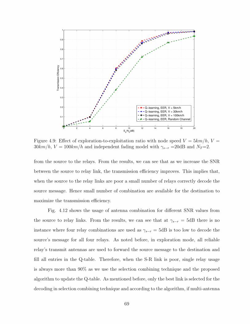
0 2 4 6 8 10 12 14 16 18 200

0.1

0.2

0.3

0.4

0.5

0.6

0.7

0.8

0.9

1

Eb/N

0(dB)

Tra

nsm

issio

n E

ffic

iency

Q−learning, EER, V = 5km/h



Q−learning, EER, Random Channel

Figure 4.9: Effect of exploration-to-exploitation ratio with node speed V = 5km/h, V =30km/h, V = 100km/h and independent fading model with γs−r =20dB and NT=2.

from the source to the relays. From the results, we can see that as we increase the SNR

between the source to relay link, the transmission efficiency improves. This implies that,

when the source to the relay links are poor a small number of relays correctly decode the

source message. Hence small number of combination are available for the destination to

maximize the transmission efficiency.

Fig. 4.12 shows the usage of antenna combination for different SNR values from

the source to relay links. From the results, we can see that at γs−r = 5dB there is no

instance where four relay combinations are used as γs−r = 5dB is too low to decode the

source’s message for all four relays. As noted before, in exploration mode, all reliable

relay’s transmit antennas are used to forward the source message to the destination and

fill all entries in the Q-table. Therefore, when the S-R link is poor, single relay usage

is always more than 90% as we use the selection combining technique and the proposed

algorithm to update the Q-table. As mentioned before, only the best link is selected for the

decoding in selection combining technique and according to the algorithm, if multi-antenna

69

0 4 8 12 16 200

50

100

0 4 8 12 16 200

50

100

0 4 8 12 16 200

50

100

0 4 8 12 16 200

20

40

60

80

100

Perc

enta

ge u

sage o

f ante

nna c

om

bin

ation (

%)

Eb/N

0 (dB)

1 Antenna 2 Antennas 3 Antennas 4 Antennas 5 Antenna 6 Antennas 7 Antennas 8 Antennas

V = 5 km/h

V = 30 km/h

V = 100 km/h

Random

Figure 4.10: Usage of antenna combination for EER on Q-learning when channels are

Jake’s Rayleigh fading channel with node speed V = 5km/h, V = 30km/h, V = 100km/hand EER on Q-learning when channels are random. γs−r =20dB and NT=2.

70

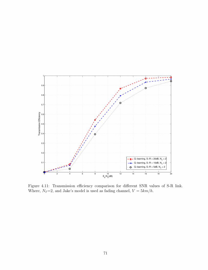
0 2 4 6 8 10 12 14 16 18 200

0.1

0.2

0.3

0.4

0.5

0.6

0.7

0.8

0.9

1

Eb/N

0(dB)

Tra

nsm

issio

n E

ffic

iency

Q−learning, S−R = 20dB, NT = 2



Figure 4.11: Transmission efficiency comparison for different SNR values of S-R link.Where, NT=2, and Jake’s model is used as fading channel, V = 5km/h.

71

0 4 8 12 16 200

50

100

0 4 8 12 16 200

50

100

0 4 8 12 16 200

50

100

Pe

rce

nta

ge

usa

ge

of

an

ten

na

co

mb

ina

tio

n (

%)

Eb/N

0 (dB)

1 Antenna 2 Antennas 3 Antennas 4 Antennas 5 Antenna 6 Antennas 7 Antennas 8 Antennas

γs−r

= 20dB

γs−r

= 10dB

γs−r

= 5dB

Figure 4.12: Usage of antenna combination for different SNR values of S-R link. Where,

Jake’s model is used as fading channel, V = 5km/h.

combination is selected by exploitation mode, then the destination not only updates it’s

specific combination but also updates all possible single antenna combinations by the

estimate of Q-values. This helps the destination to choose the proper combination for the

next packet transmission to maximize the link layer throughput by realizing the memory

introduced by the fading channel model.

4.6 Conclusions

In this chapter, we have presented the Q-learning based cross-layer relay’s transmit

antenna selection scheme to maximize the link layer transmission efficiency. The proposed

learning algorithm utilizes the memory introduced by the time-varying Rayleigh fading

channel to learn and act on future relay selections and hence, improved throughput max-

imization relative to the conventional schemes with no learning involved. We have shown

72

that when relays are equipped with multiple transmit antennas the throughput perfor-

mance outperforms the case with single transmit antenna. The performance of transmit

antenna selection has been studied in this work. We have presented and compared the

throughput performance with and without transmit antenna selection. The impact of the

number of cooperating relays have been studied, where we have shown that as the number

of cooperating relays increases, the throughput performance improves. Furthermore, the

throughput performance for different source to relay link qualities has been studied. Re-

sults have shown that as the channel quality gets poorer, less reliable relays are available

and the system throughput degrades. Our proposed system utilizes the channel resources

more efficiently than the existing systems.

73

Chapter 5

Conclusions and Future Works

5.1 Conclusions

In this thesis we focused on studying the performance of cooperative relay networks.

First we briefly reviewed cooperative diversity, different diversity combining techniques,

Jake’s Rayleigh fading model and an introduction on reinforcement learning. Throughout

the thesis, we proved that using learning algorithms, reliable relay and reliable relay’s

antenna selection improve the performance of the cooperative network.

In chapter 3, the performance of Q-learning based cross-layer relay selection scheme

was analyzed to maximize the link layer transmission efficiency. We studied the case for

both time-varying Rayleigh fading channel modeled as Jake’s model and also for indepen-

dent fading model. We showed that, the proposed learning algorithm utilizes the memory

introduced by the time-varying Rayleigh fading channel to learn and act on future relay

selection to improve throughput performance relative to schemes where no learning is

involved. We also have shown the effect of exploration-to-exploitation ratio, where the

algorithm offers transmission efficiency gain over systems utilizing ε greedy mechanism.

In addition to that, our proposed system uses the bandwidth efficiently as the algorithm

chooses few number of reliable relays to maximize the throughput.

74

In chapter 4, multiple transmit antennas are considered for the relay nodes to

analyze the Q-learning based cross-layer relay’s transmit antennas selection scheme to

maximize the link layer transmission efficiency. The performance of the network was

studied for both the ε greedy mechanism and the optimized exploration-to-exploitation

ratio using the Q-learning based relay’s transmit antennas selection. We have shown

that, the throughput performance of multiple transmit antennas employed in the relay

node outperform the case when the relays are equipped with single transmit antenna. We

also have presented and compared the throughput performance with and without transmit

antenna selection. The impact of the number of cooperating relays has been examined,

where we have shown that as the number of cooperating relays increases the throughput

performance improves. Furthermore, the throughput performance for different source to

relay link qualities has also studied. Results show that as the channel quality gets poorer

the system employs less relays and hence system throughput degrades. We also found

that, our proposed system utilizes the channel resources more efficiently and also provides

improved transmission efficiency.

5.2 Future Works

In the sequel, here, we list some of the topics of interest.

1. In Chapter 3 and 4, we have considered cooperative networks operating in a par-

ticular frequency channel at a particular time instant. But, nodes can operate in

multiple frequency channels simultaneously instead of adopting a single channel.

Channel allocation problem for such system is an important research direction.

2. In our study we haven’t used any channel coding techniques. Therefore, a study of

the improvements when employing powerful channel codes such as turbo code is of

75

great interest.

3. The proposed cross-layer schemes are aimed at cognitive networks where learning

techniques are a major part of such networks. However, our study was more gen-

eral where it can be used for any cooperative system with some powerful nodes

that can accommodate learning techniques. It is of interest to study the proposed

cross-layer schemes in a cognitive network setting where both primary and cognitive

(secondary) users exits.

4. Also, our proposed cross-layer schemes require additional computations and storage

to perform Q-learning. A computational study would also be interesting to compare

with conventional (i.e, no learning) techniques.

76

Bibliography

[1] T. M. Duman and A. Ghrayeb, Coding for MIMO communication systems. Wiley

Online Library, 2007.

[2] J. G. Proakis, Digital Communications. New York:McGraw-Hill, 2001.

[3] D. G. A. Paulraj, R. Nabar, Introduction to Space-Time Wireless Communications.

Cambridge University press, 2003.

[4] W. L. M.-i. L. D. M. B. C. Q. Li, G. Li and Z. Li., “MIMO techniques in WiMAX

and LTE: a feature overview,” IEEE Communications Magazine, vol. 48, no. 5, pp.

86–92, 2010.

[5] E. C. L. Charfi and L. Kamou, “PHY/MAC enhancements and QoS mechanisms

for very high throughput WLANs: A survey,” IEEE Communications Surveys &

Tutorials, vol. 15, no. 4, pp. 1714–1735, 2013.

[6] E. van der Muelen, “Three-terminal communication channels,” Adv. Appl. Probab,

vol. 3, pp. 120–154, 1971.

[7] A. J. G. S. Cui and A. Bahai, “Energy-efficiency of mimo and cooperative mimo in

sensor networks,” IEEE Journal on Selected Areas in Communications, vol. 22, p.

10891098, 2008.

[8] J. N. Laneman, D. N. Tse, and G. W. Wornell, “Cooperative diversity in wireless net-

77

works: Efficient protocols and outage behavior,” IEEE Transactions on Information

Theory, vol. 50, no. 12, pp. 3062–3080, 2004.

[9] L. Dai and K. Letaief, “Throughput maximization of ad-hoc wireless networks using

adaptive cooperative diversity and truncated ARQ,” IEEE Transactions on Commu-

nications, vol. 56, no. 11, pp. 1907–1918, 2008.

[10] Y. Zhao, R. Adve, and T. J. Lim, “Symbol error rate of selection amplify-and-forward

relay systems,” IEEE Communications Letters, vol. 10, no. 11, pp. 757–759, 2006.

[11] E. Koyuncu, Y. Jing, and H. Jafarkhani, “Distributed beamforming in wireless relay

networks with quantized feedback,” IEEE Journal on Selected Areas in Communica-

tions, vol. 26, no. 8, pp. 1429–1439, 2008.

[12] A. Sendonaris, E. Erkip, and B. Aazhang, “User cooperation diversity. Part I. System

description,” IEEE Transactions on Communications, vol. 51, no. 11, pp. 1927–1938,

2003.

[13] J. N. Laneman and G. W. Wornell, “Distributed space-time-coded protocols for ex-

ploiting cooperative diversity in wireless networks,” IEEE Transactions on Informa-

tion Theory, vol. 49, no. 10, pp. 2415–2425, 2003.

[14] M. Patzold and F. Laue, “Statistical properties of jakes’ fading channel simulator,”

in Vehicular Technology Conference, 1998. VTC 98. 48th IEEE, vol. 2. IEEE, 1998,

pp. 712–718.

[15] G. L. Stuber, Principles of Mobile Communication, T. Edition, Ed., 2012.

[16] E. Alpaydin, Introduction to machine learning. MIT press, 2004.

[17] T. M. N. K., “Learning automata - a survey,” IEEE Transactions on Systems, Man,

and Cybernetics, vol. SMC-4, no. 4, pp. 323–334, 1974.

78

[18] “Report of the spectrum efficiency working group,” FCC, Washington, DC, Tech.

Rep., Tech. Rep. 02-135, Nov. 2002.

[19] L. M. M. A. Kaelbling, L.P., “einforcement learning: a survey,” J. Artif. Intell. Res.,

pp. 237–287, 1996.

[20] D. G. T. Jiang and P. Mitchel, “Efficient exploration in reinforcement learning-based

cognitive radio spectrum sharing,” IET Communications, vol. 5, no. 10, pp. 1309–

1317, 2011.

[21] M. D. F. C. Wu, K. Chowdhury and W. Melei, “Spectrum management of cognitive

radio using multi-agent reinforcement learning,” in 9th International Conference on

Autonomous Agents and Multiagent Systems: Industry track, 2010.

[22] B. Lo and I. Akyildiz, “Reinforcement learning-based cooperative sensing in cogni-

tive radio ad hoc networks,” in Personal Indoor and Mobile Radio Communications

(PIMRC), 2010 IEEE 21st International Symposium on, 2010, pp. 2244–2249.

[23] D. G. T. Jiang and P. Mitchell, “Efficient exploration in reinforcement learning-based

cognitive radio spectrum sharing,” IET Communications, vol. 5, no. 10, pp. 1309–

1317, 2011.

[24] S. M. C. T. Tan, C.K., “Game theoretic approach for channel assignment and power

control with no-internal-regret learning in wireless ad hoc networks,” IET Commu-

nications, vol. 2, no. 9, pp. 1159–1169, 2008.

[25] S. R. N. M. Neihart and D. J. Allsto, “A Parallel, Multi-Resolution Sensing Technique

for Multiple Antenna Cognitive Radios,” in Circuits and Systems, 2007. ISCAS 2007.

IEEE International Symposium on, 2007, pp. 2530–2533.

[26] Y.-C. L. Feifei Gao, Rui Zhang and X. Wang, “Design of learning-based MIMO

cognitive radio systems,” vol. 59, no. 4, pp. 1707–1720, 2010.

79

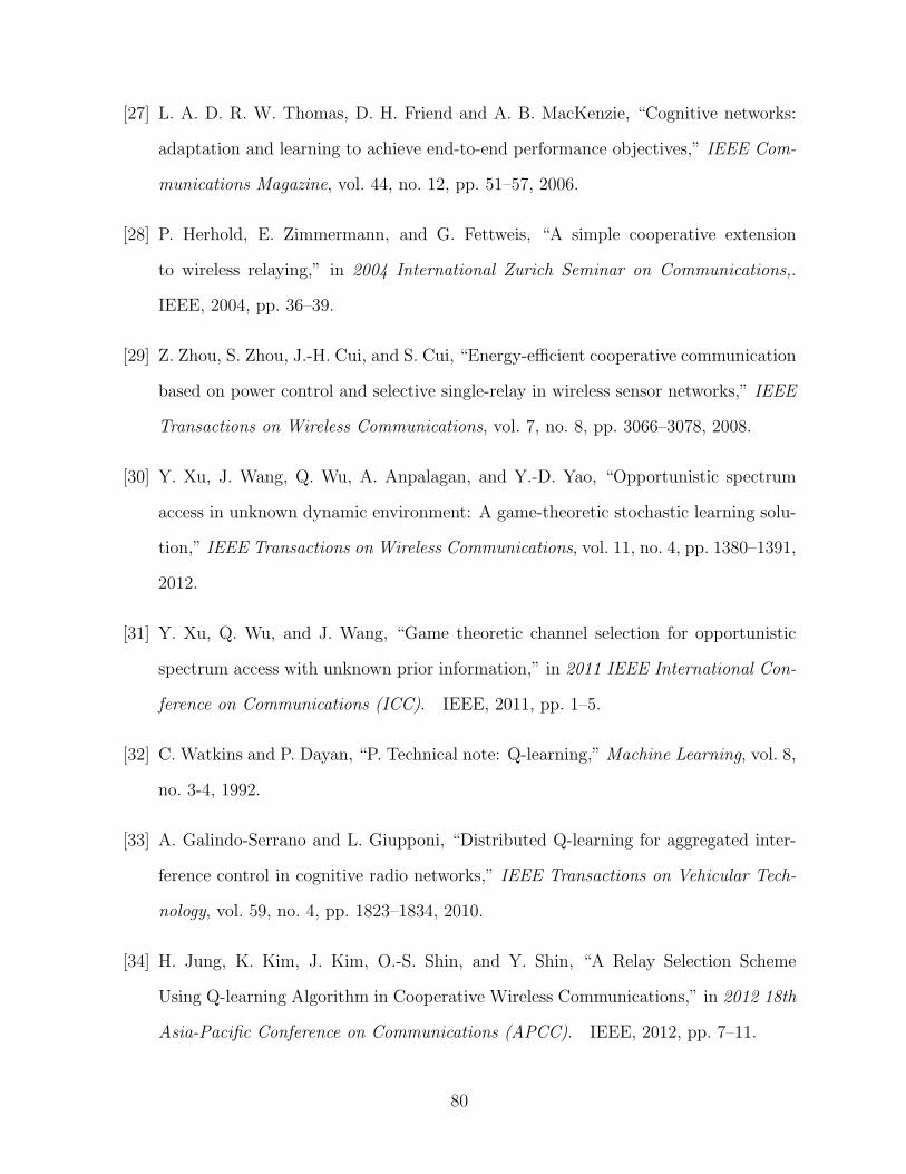
[27] L. A. D. R. W. Thomas, D. H. Friend and A. B. MacKenzie, “Cognitive networks:

adaptation and learning to achieve end-to-end performance objectives,” IEEE Com-

munications Magazine, vol. 44, no. 12, pp. 51–57, 2006.

[28] P. Herhold, E. Zimmermann, and G. Fettweis, “A simple cooperative extension

to wireless relaying,” in 2004 International Zurich Seminar on Communications,.

IEEE, 2004, pp. 36–39.

[29] Z. Zhou, S. Zhou, J.-H. Cui, and S. Cui, “Energy-efficient cooperative communication

based on power control and selective single-relay in wireless sensor networks,” IEEE

Transactions on Wireless Communications, vol. 7, no. 8, pp. 3066–3078, 2008.

[30] Y. Xu, J. Wang, Q. Wu, A. Anpalagan, and Y.-D. Yao, “Opportunistic spectrum

access in unknown dynamic environment: A game-theoretic stochastic learning solu-

tion,” IEEE Transactions on Wireless Communications, vol. 11, no. 4, pp. 1380–1391,

2012.

[31] Y. Xu, Q. Wu, and J. Wang, “Game theoretic channel selection for opportunistic

spectrum access with unknown prior information,” in 2011 IEEE International Con-

ference on Communications (ICC). IEEE, 2011, pp. 1–5.

[32] C. Watkins and P. Dayan, “P. Technical note: Q-learning,” Machine Learning, vol. 8,

no. 3-4, 1992.

[33] A. Galindo-Serrano and L. Giupponi, “Distributed Q-learning for aggregated inter-

ference control in cognitive radio networks,” IEEE Transactions on Vehicular Tech-

nology, vol. 59, no. 4, pp. 1823–1834, 2010.

[34] H. Jung, K. Kim, J. Kim, O.-S. Shin, and Y. Shin, “A Relay Selection Scheme

Using Q-learning Algorithm in Cooperative Wireless Communications,” in 2012 18th

Asia-Pacific Conference on Communications (APCC). IEEE, 2012, pp. 7–11.

80

[35] P. Liu, Z. Tao, S. Narayanan, T. Korakis, and S. S. Panwar, “CoopMAC: A coopera-

tive MAC for wireless LANs,” IEEE Journal on Selected Areas in Communications,

vol. 25, no. 2, pp. 340–354, 2007.

[36] Q. Zhao and H. Li, “Performance of differential modulation with wireless relays in

rayleigh fading channels,” Communications Letters, IEEE, vol. 9, no. 4, pp. 343–345,

2005.

[37] M. R. Souryal, “Non-coherent amplify-and-forward generalized likelihood ratio test

receiver,” Wireless Communications, IEEE Transactions on, vol. 9, no. 7, pp. 2320–

2327, 2010.

[38] R. Annavajjala, P. C. Cosman, and L. B. Milstein, “On the performance of opti-

mum noncoherent amplify-and-forward reception for cooperative diversity,” in Mil-

itary Communications Conference, 2005. MILCOM 2005. IEEE. IEEE, 2005, pp.

3280–3288.

[39] E. Rodrigues Gomes and R. Kowalczyk, “Dynamic analysis of multiagent Q-learning

with ε-greedy exploration,” in Proceedings of the 26th Annual International Confer-

ence on Machine Learning. ACM, 2009, pp. 369–376.

[40] K. Fazel and S. Kaiser, Multi-Carrier and Spread Spectrum Systems: From OFDM

and MC-CDMA to LTE and WiMAX. John Wiley & Sons., 2008.

[41] H. C. K. Yang, S. Ou and J. He, “A multihop peer-communication protocol with

fairness guarantee for IEEE 802.16-based vehicular networks,” IEEE transactions on

vechicular technologys, vol. 56, no. 6, pp. 3358–3370, 2007.

[42] K. G. K. Yang, S. Ou and H.-H. Chen, “Convergence of ethernet PON and IEEE

802.16 broadband access networks and its QoS-aware dynamic bandwidth allocation

scheme,” IEEE Journal on Selected Areas in Communications, vol. 27, no. 2, pp.

101–116, 2009.

81

[43] G. J. Foschini and M. J. Gans, “On limits of wireless communications in a fading

environment when using multiple antennas,” Wireless Personal Commun., vol. 6, p.

311335, 1998.

[44] H. W. C.-X. Wang, X. Hong and W. X, “Spatial temporal correlation properties of the

3GPP spatial channel model and the Kronecker MIMO channel model,” EURASIP

J. Wireless Commun. and Networking, p. 9 pages, 2007.

[45] G. J. Foschini, “Layered space-time architecture for wireless communication in fading

environments when using multi- element antennas,” Bell Labs Tech. J.(2), pp. 41–59,

1996.

[46] S. M. Alamouti, “A simple transmit diversity technique for wireless communications,”

IEEE Journal on Selected Areas in Communications, vol. 16, no. 8, pp. 1451–1458,

1998.

[47] N. S. V. Tarokh and A. Calderbank, “Space-time codes for high data rate wireless

communication: Perfor- mance criteria and code construction,” IEEE Trans. Inform.

Theory, (2), pp. 744765,, March, 1998.

[48] C. Z. S. Jin, M. R. McKay and K.-K. Wong, “Ergodic capacity analysis of amplify-

and-forward MIMO dual-hop systems,” IEEE Trans. Inf. Theory, vol. 56, pp. 1903–

1907, 2008.

[49] W. E. S. Sungjoon Park, “Opportunistic dual timer relay selection in MIMO relay

networks,” in Military Communications Conference, 2012 - MILCOM 2012, 2012,

pp. 1–6.

[50] R. U. N. D. A. Gore and A. J. Paulrj, “Selecting an optimal set of transmit antennas

for a low rank matrix channel,” in Acoustics, Speech, and Signal Processing, 2000.

ICASSP ’00. Proceedings. 2000 IEEE International Conference on, vol. 5, 2000, pp.

2785–2788.

82

[51] H. S. Z. Tang and I. B. Collings, “Performance of 802.11n WLAN with transmit an-

tenna selection in measured indoor channels,” in Communications Theory Workshop,

2008. AusCTW 2008. Australian, 2008, pp. 139–143.

[52] N. Nie and C. Comanici, “Adaptive channel allocation spectrum etiquette for cogni-

tive radio networks,” in New Frontiers in Dynamic Spectrum Access Networks, 2005.

DySPAN 2005. 2005 First IEEE International Symposium on, 2005, pp. 269–278.

[53] P. K. K.-L. A. Yau and P. D. Teal, “Context-awareness and intelligence in distributed

cognitive radio networks: A reinforcement learning approach,” in Communications

Theory Workshop (AusCTW), 2010 Australian, 2010, pp. 35–42.

[54] P. Venkatraman and B. Hamdaou, “Cooperative q-learning for multiple secondary

users in dynamic spectrum access,” in Wireless Communications and Mobile Com-

puting Conference (IWCMC), 2011 7th International, 2011, pp. 238–242.

[55] H. Li, “Multi-agent q-learning of channel selection in multi-user cognitive radio sys-

tems: A two by two case,” in Systems, Man and Cybernetics, 2009. SMC 2009. IEEE

International Conference on, 2009, pp. 1893–1898.

[56] A. Ghosh and W. Hamouda, “Channel selection for heterogeneous nodes in cognitive

networks,” in Communications (ICC), 2013 IEEE International Conference on, 2013,

pp. 5939–5943.

83

learning based relay and antenna selection in cooperative ... · learning based relay and antenna...

Documents