learning apache spark with pythonweb.utk.edu/~wfeng1/doc/pyspark.pdf · spark runs on hadoop,...
TRANSCRIPT
Learning Apache Spark with PythonRelease v1.0
Wenqiang Feng
February 18, 2019

CONTENTS
1 Preface 21.1 About . . . . . . . . . . . . . . . . . . . . . . . . . . . . . . . . . . . . . . . . . . . . 21.2 Motivation for this tutorial . . . . . . . . . . . . . . . . . . . . . . . . . . . . . . . . . 31.3 Copyright notice and license info . . . . . . . . . . . . . . . . . . . . . . . . . . . . . 31.4 Acknowledgement . . . . . . . . . . . . . . . . . . . . . . . . . . . . . . . . . . . . . 31.5 Feedback and suggestions . . . . . . . . . . . . . . . . . . . . . . . . . . . . . . . . . 4
2 Why Spark with Python ? 52.1 Why Spark? . . . . . . . . . . . . . . . . . . . . . . . . . . . . . . . . . . . . . . . . 52.2 Why Spark with Python (PySpark)? . . . . . . . . . . . . . . . . . . . . . . . . . . . . 6
3 Configure Running Platform 83.1 Run on Databricks Community Cloud . . . . . . . . . . . . . . . . . . . . . . . . . . . 83.2 Configure Spark on Mac and Ubuntu . . . . . . . . . . . . . . . . . . . . . . . . . . . 123.3 Configure Spark on Windows . . . . . . . . . . . . . . . . . . . . . . . . . . . . . . . 153.4 PySpark With Text Editor or IDE . . . . . . . . . . . . . . . . . . . . . . . . . . . . . 153.5 PySparkling Water: Spark + H2O . . . . . . . . . . . . . . . . . . . . . . . . . . . . . 173.6 Set up Spark on Cloud . . . . . . . . . . . . . . . . . . . . . . . . . . . . . . . . . . . 193.7 Demo Code in this Section . . . . . . . . . . . . . . . . . . . . . . . . . . . . . . . . . 19
4 An Introduction to Apache Spark 214.1 Core Concepts . . . . . . . . . . . . . . . . . . . . . . . . . . . . . . . . . . . . . . . 214.2 Spark Components . . . . . . . . . . . . . . . . . . . . . . . . . . . . . . . . . . . . . 214.3 Architecture . . . . . . . . . . . . . . . . . . . . . . . . . . . . . . . . . . . . . . . . 244.4 How Spark Works? . . . . . . . . . . . . . . . . . . . . . . . . . . . . . . . . . . . . . 24
5 Programming with RDDs 255.1 Create RDD . . . . . . . . . . . . . . . . . . . . . . . . . . . . . . . . . . . . . . . . 255.2 Spark Operations . . . . . . . . . . . . . . . . . . . . . . . . . . . . . . . . . . . . . . 28
6 Statistics Preliminary 316.1 Notations . . . . . . . . . . . . . . . . . . . . . . . . . . . . . . . . . . . . . . . . . . 316.2 Measurement Formula . . . . . . . . . . . . . . . . . . . . . . . . . . . . . . . . . . . 316.3 Statistical Tests . . . . . . . . . . . . . . . . . . . . . . . . . . . . . . . . . . . . . . . 32
7 Data Exploration 337.1 Univariate Analysis . . . . . . . . . . . . . . . . . . . . . . . . . . . . . . . . . . . . 337.2 Multivariate Analysis . . . . . . . . . . . . . . . . . . . . . . . . . . . . . . . . . . . . 45
8 Regression 49
i
8.1 Linear Regression . . . . . . . . . . . . . . . . . . . . . . . . . . . . . . . . . . . . . 498.2 Generalized linear regression . . . . . . . . . . . . . . . . . . . . . . . . . . . . . . . 578.3 Decision tree Regression . . . . . . . . . . . . . . . . . . . . . . . . . . . . . . . . . . 638.4 Random Forest Regression . . . . . . . . . . . . . . . . . . . . . . . . . . . . . . . . . 688.5 Gradient-boosted tree regression . . . . . . . . . . . . . . . . . . . . . . . . . . . . . . 73
9 Regularization 799.1 Ordinary least squares regression . . . . . . . . . . . . . . . . . . . . . . . . . . . . . 799.2 Ridge regression . . . . . . . . . . . . . . . . . . . . . . . . . . . . . . . . . . . . . . 799.3 Least Absolute Shrinkage and Selection Operator (LASSO) . . . . . . . . . . . . . . . 809.4 Elastic net . . . . . . . . . . . . . . . . . . . . . . . . . . . . . . . . . . . . . . . . . 80
10 Classification 8110.1 Binomial logistic regression . . . . . . . . . . . . . . . . . . . . . . . . . . . . . . . . 8110.2 Multinomial logistic regression . . . . . . . . . . . . . . . . . . . . . . . . . . . . . . 8910.3 Decision tree Classification . . . . . . . . . . . . . . . . . . . . . . . . . . . . . . . . 9910.4 Random forest Classification . . . . . . . . . . . . . . . . . . . . . . . . . . . . . . . . 10610.5 Gradient-boosted tree Classification . . . . . . . . . . . . . . . . . . . . . . . . . . . . 11310.6 XGBoost: Gradient-boosted tree Classification . . . . . . . . . . . . . . . . . . . . . . 11410.7 Naive Bayes Classification . . . . . . . . . . . . . . . . . . . . . . . . . . . . . . . . . 116
11 Clustering 12611.1 K-Means Model . . . . . . . . . . . . . . . . . . . . . . . . . . . . . . . . . . . . . . 126
12 RFM Analysis 13412.1 RFM Analysis Methodology . . . . . . . . . . . . . . . . . . . . . . . . . . . . . . . . 13512.2 Demo . . . . . . . . . . . . . . . . . . . . . . . . . . . . . . . . . . . . . . . . . . . . 13712.3 Extension . . . . . . . . . . . . . . . . . . . . . . . . . . . . . . . . . . . . . . . . . . 141
13 Text Mining 14713.1 Text Collection . . . . . . . . . . . . . . . . . . . . . . . . . . . . . . . . . . . . . . . 14713.2 Text Preprocessing . . . . . . . . . . . . . . . . . . . . . . . . . . . . . . . . . . . . . 15313.3 Text Classification . . . . . . . . . . . . . . . . . . . . . . . . . . . . . . . . . . . . . 15613.4 Sentiment analysis . . . . . . . . . . . . . . . . . . . . . . . . . . . . . . . . . . . . . 16113.5 N-grams and Correlations . . . . . . . . . . . . . . . . . . . . . . . . . . . . . . . . . 16713.6 Topic Model: Latent Dirichlet Allocation . . . . . . . . . . . . . . . . . . . . . . . . . 167
14 Social Network Analysis 17814.1 Introduction . . . . . . . . . . . . . . . . . . . . . . . . . . . . . . . . . . . . . . . . 17814.2 Co-occurrence Network . . . . . . . . . . . . . . . . . . . . . . . . . . . . . . . . . . 17814.3 Appendix: matrix multiplication in PySpark . . . . . . . . . . . . . . . . . . . . . . . 18214.4 Correlation Network . . . . . . . . . . . . . . . . . . . . . . . . . . . . . . . . . . . . 183
15 ALS: Stock Portfolio Recommendations 18415.1 Recommender systems . . . . . . . . . . . . . . . . . . . . . . . . . . . . . . . . . . . 18515.2 Alternating Least Squares . . . . . . . . . . . . . . . . . . . . . . . . . . . . . . . . . 18515.3 Demo . . . . . . . . . . . . . . . . . . . . . . . . . . . . . . . . . . . . . . . . . . . . 185
16 Monte Carlo Simulation 19216.1 Simulating Casino Win . . . . . . . . . . . . . . . . . . . . . . . . . . . . . . . . . . . 19216.2 Simulating a Random Walk . . . . . . . . . . . . . . . . . . . . . . . . . . . . . . . . 193
17 Markov Chain Monte Carlo 201
ii

18 Neural Network 20218.1 Feedforward Neural Network . . . . . . . . . . . . . . . . . . . . . . . . . . . . . . . 202
19 My PySpark Package 20519.1 Hierarchical Structure . . . . . . . . . . . . . . . . . . . . . . . . . . . . . . . . . . . 20519.2 Set Up . . . . . . . . . . . . . . . . . . . . . . . . . . . . . . . . . . . . . . . . . . . 20619.3 ReadMe . . . . . . . . . . . . . . . . . . . . . . . . . . . . . . . . . . . . . . . . . . . 206
20 Main Reference 208
Bibliography 209
Index 211
iii

iv

Learning Apache Spark with Python, Release v1.0
Welcome to my Learning Apache Spark with Python note! In this note, you will learn a wide arrayof concepts about PySpark in Data Mining, Text Mining, Machine Leanring and Deep Learning. ThePDF version can be downloaded from HERE.
CONTENTS 1
CHAPTER
ONE
PREFACE
1.1 About
1.1.1 About this note
This is a shared repository for Learning Apache Spark Notes. The PDF version can bedownloaded from HERE. The first version was posted on Github in ChenFeng ([Feng2017]).This shared repository mainly contains the self-learning and self-teaching notes from Wen-qiang during his IMA Data Science Fellowship. The reader is referred to the repositoryhttps://github.com/runawayhorse001/LearningApacheSpark for more details about the dataset andthe .ipynb files.
In this repository, I try to use the detailed demo code and examples to show how to use each mainfunctions. If you find your work wasn’t cited in this note, please feel free to let me know.
Although I am by no means an data mining programming and Big Data expert, I decided that it wouldbe useful for me to share what I learned about PySpark programming in the form of easy tutorials withdetailed example. I hope those tutorials will be a valuable tool for your studies.
The tutorials assume that the reader has a preliminary knowledge of programing and Linux. And thisdocument is generated automatically by using sphinx.
1.1.2 About the authors
• Wenqiang Feng
– Data Scientist and PhD in Mathematics
– University of Tennessee at Knoxville
– Email: [email protected]
• Biography
Wenqiang Feng is Data Scientist within DST’s Applied Analytics Group. Dr. Feng’s responsibil-ities include providing DST clients with access to cutting-edge skills and technologies, includingBig Data analytic solutions, advanced analytic and data enhancement techniques and modeling.
Dr. Feng has deep analytic expertise in data mining, analytic systems, machine learning algo-rithms, business intelligence, and applying Big Data tools to strategically solve industry problemsin a cross-functional business. Before joining DST, Dr. Feng was an IMA Data Science Fellow atThe Institute for Mathematics and its Applications (IMA) at the University of Minnesota. Whilethere, he helped startup companies make marketing decisions based on deep predictive analytics.
2
Learning Apache Spark with Python, Release v1.0
Dr. Feng graduated from University of Tennessee, Knoxville, with Ph.D. in Computational Math-ematics and Master’s degree in Statistics. He also holds Master’s degree in Computational Math-ematics from Missouri University of Science and Technology (MST) and Master’s degree in Ap-plied Mathematics from the University of Science and Technology of China (USTC).
• Declaration
The work of Wenqiang Feng was supported by the IMA, while working at IMA. However, anyopinion, finding, and conclusions or recommendations expressed in this material are those of theauthor and do not necessarily reflect the views of the IMA, UTK and DST.
1.2 Motivation for this tutorial
I was motivated by the IMA Data Science Fellowship project to learn PySpark. After that I was im-pressed and attracted by the PySpark. And I foud that:
1. It is no exaggeration to say that Spark is the most powerful Bigdata tool.
2. However, I still found that learning Spark was a difficult process. I have to Google it and identifywhich one is true. And it was hard to find detailed examples which I can easily learned the fullprocess in one file.
3. Good sources are expensive for a graduate student.
1.3 Copyright notice and license info
This Learning Apache Spark with Python PDF file is supposed to be afree and living document, which is why its source is available online athttps://runawayhorse001.github.io/LearningApacheSpark/pyspark.pdf. But this document is li-censed according to both MIT License and Creative Commons Attribution-NonCommercial 2.0 Generic(CC BY-NC 2.0) License.
When you plan to use, copy, modify, merge, publish, distribute or sublicense, Please see the termsof those licenses for more details and give the corresponding credits to the author.
1.4 Acknowledgement
At here, I would like to thank Ming Chen, Jian Sun and Zhongbo Li at the University of Tennesseeat Knoxville for the valuable disscussion and thank the generous anonymous authors for providing thedetailed solutions and source code on the internet. Without those help, this repository would not havebeen possible to be made. Wenqiang also would like to thank the Institute for Mathematics and ItsApplications (IMA) at University of Minnesota, Twin Cities for support during his IMA Data ScientistFellow visit.
A special thank you goes to Dr. Haiping Lu, Lecturer in Machine Learning at Department of ComputerScience, University of Sheffield, for recommending and heavily using my tutorial in his teaching classand for the valuable suggestions.
1.2. Motivation for this tutorial 3
Learning Apache Spark with Python, Release v1.0
1.5 Feedback and suggestions
Your comments and suggestions are highly appreciated. I am more than happy to receive corrections,suggestions or feedbacks through email ([email protected]) for improvements.
4 Chapter 1. Preface
CHAPTER
TWO
WHY SPARK WITH PYTHON ?
Chinese proverb
Sharpening the knife longer can make it easier to hack the firewood – old Chinese proverb
I want to answer this question from the following two parts:
2.1 Why Spark?
I think the following four main reasons from Apache Spark™ official website are good enough to con-vince you to use Spark.
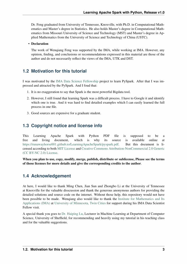
1. Speed
Run programs up to 100x faster than Hadoop MapReduce in memory, or 10x faster on disk.
Apache Spark has an advanced DAG execution engine that supports acyclic data flow and in-memory computing.
Figure 2.1: Logistic regression in Hadoop and Spark
2. Ease of Use
Write applications quickly in Java, Scala, Python, R.
Spark offers over 80 high-level operators that make it easy to build parallel apps. And you can useit interactively from the Scala, Python and R shells.
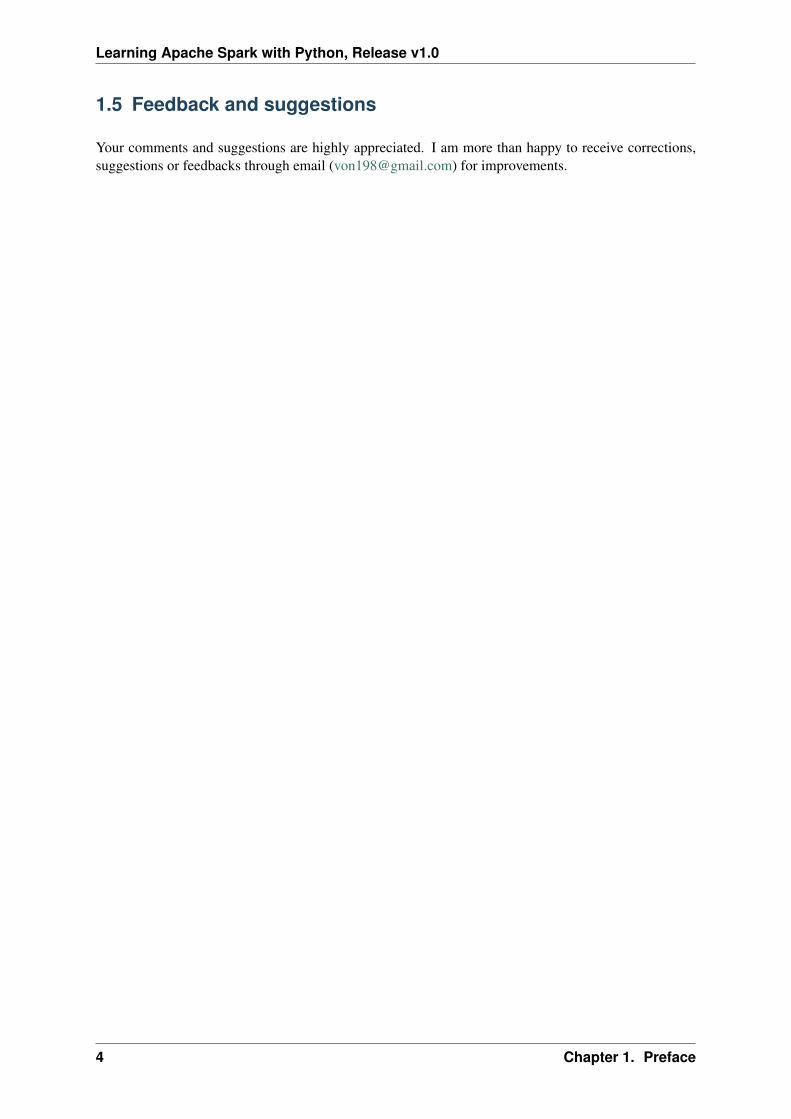
3. Generality
Combine SQL, streaming, and complex analytics.
5
Learning Apache Spark with Python, Release v1.0
Spark powers a stack of libraries including SQL and DataFrames, MLlib for machine learning,GraphX, and Spark Streaming. You can combine these libraries seamlessly in the same applica-tion.
Figure 2.2: The Spark stack
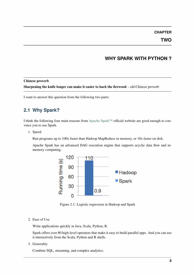
4. Runs Everywhere
Spark runs on Hadoop, Mesos, standalone, or in the cloud. It can access diverse data sourcesincluding HDFS, Cassandra, HBase, and S3.
Figure 2.3: The Spark platform
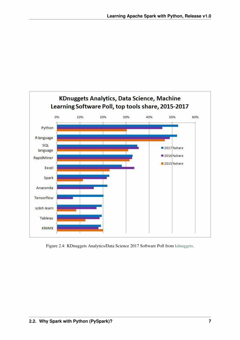
2.2 Why Spark with Python (PySpark)?
No matter you like it or not, Python has been one of the most popular programming languages.
6 Chapter 2. Why Spark with Python ?
Learning Apache Spark with Python, Release v1.0
Figure 2.4: KDnuggets Analytics/Data Science 2017 Software Poll from kdnuggets.
2.2. Why Spark with Python (PySpark)? 7
CHAPTER
THREE
CONFIGURE RUNNING PLATFORM
Chinese proverb
Good tools are prerequisite to the successful execution of a job. – old Chinese proverb
A good programming platform can save you lots of troubles and time. Herein I will only present howto install my favorite programming platform and only show the easiest way which I know to set it up onLinux system. If you want to install on the other operator system, you can Google it. In this section, youmay learn how to set up Pyspark on the corresponding programming platform and package.
3.1 Run on Databricks Community Cloud
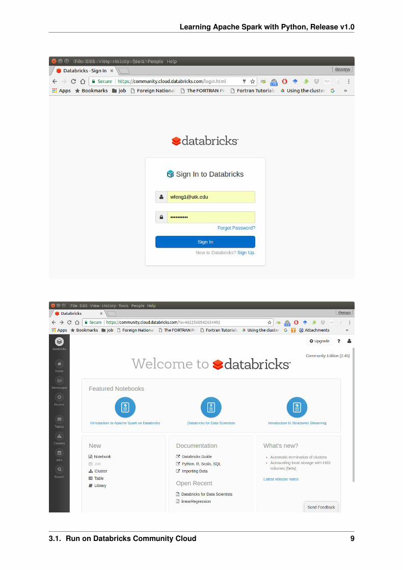
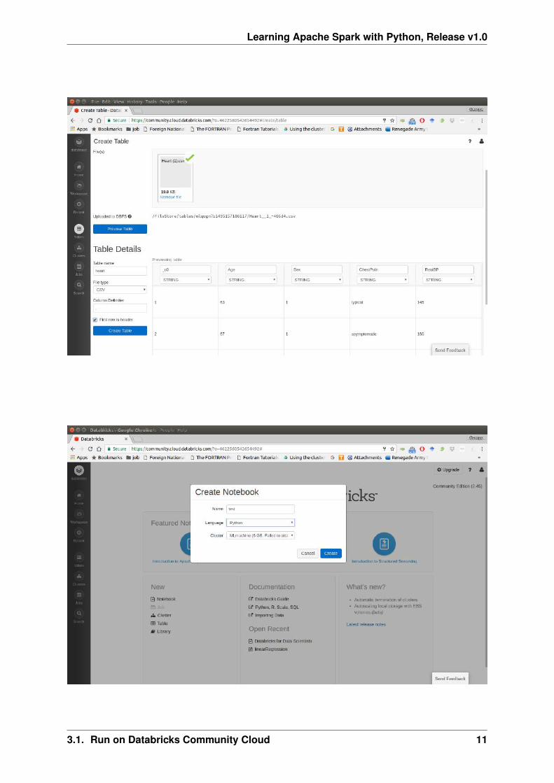
If you don’t have any experience with Linux or Unix operator system, I would love to recommend youto use Spark on Databricks Community Cloud. Since you do not need to setup the Spark and it’s totallyfree for Community Edition. Please follow the steps listed below.
1. Sign up a account at: https://community.cloud.databricks.com/login.html
2. Sign in with your account, then you can creat your cluster(machine), table(dataset)and notebook(code).
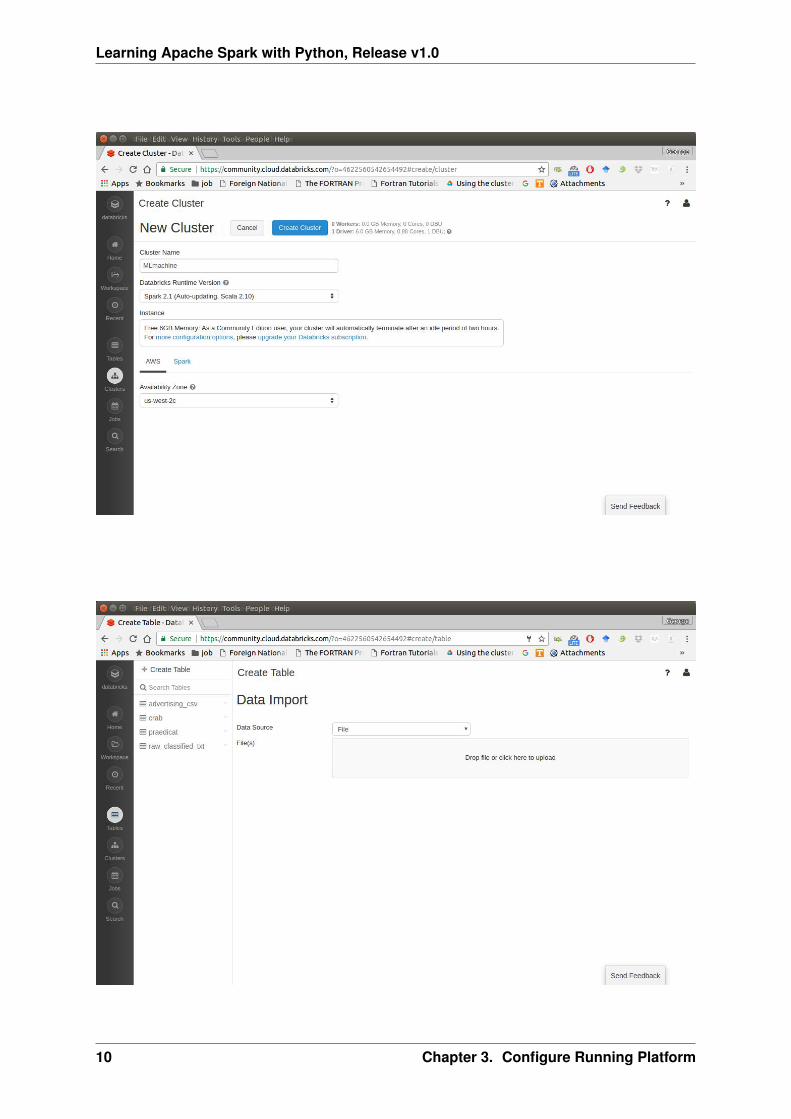
3. Create your cluster where your code will run
4. Import your dataset
Note: You need to save the path which appears at Uploaded to DBFS: /File-Store/tables/05rmhuqv1489687378010/. Since we will use this path to load the dataset.
5. Creat your notebook
After finishing the above 5 steps, you are ready to run your Spark code on Databricks Community Cloud.I will run all the following demos on Databricks Community Cloud. Hopefully, when you run the democode, you will get the following results:
8
Learning Apache Spark with Python, Release v1.0
3.1. Run on Databricks Community Cloud 9
Learning Apache Spark with Python, Release v1.0
10 Chapter 3. Configure Running Platform
Learning Apache Spark with Python, Release v1.0
3.1. Run on Databricks Community Cloud 11
Learning Apache Spark with Python, Release v1.0
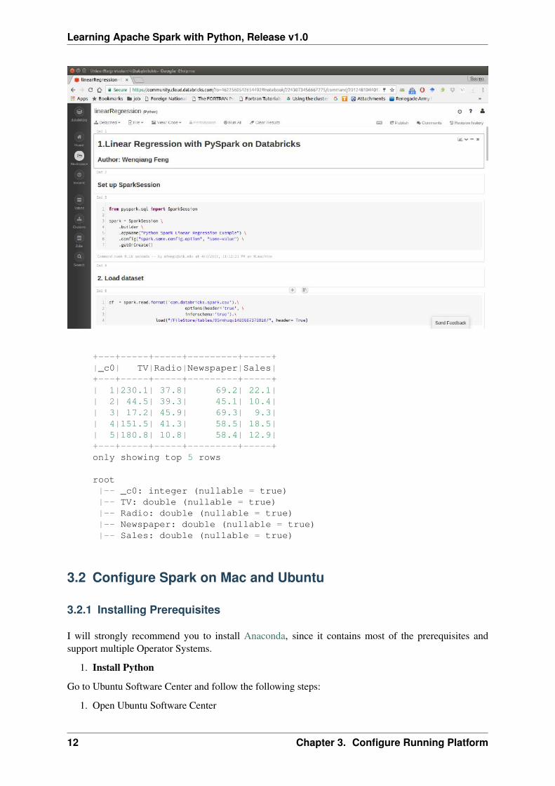
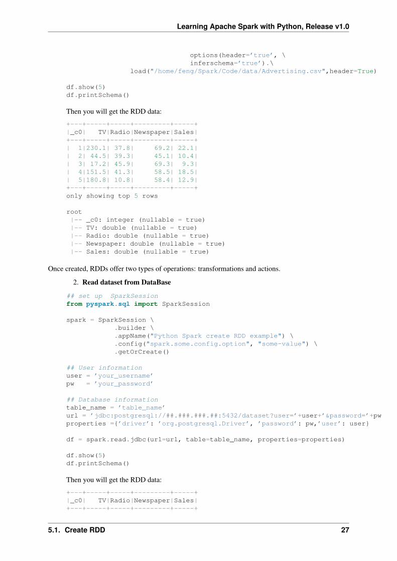
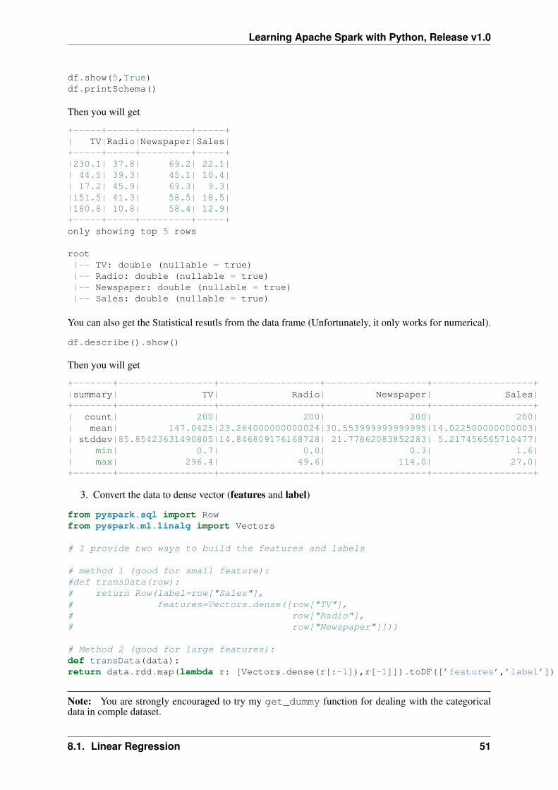
+---+-----+-----+---------+-----+|_c0| TV|Radio|Newspaper|Sales|+---+-----+-----+---------+-----+| 1|230.1| 37.8| 69.2| 22.1|| 2| 44.5| 39.3| 45.1| 10.4|| 3| 17.2| 45.9| 69.3| 9.3|| 4|151.5| 41.3| 58.5| 18.5|| 5|180.8| 10.8| 58.4| 12.9|+---+-----+-----+---------+-----+only showing top 5 rows
root|-- _c0: integer (nullable = true)|-- TV: double (nullable = true)|-- Radio: double (nullable = true)|-- Newspaper: double (nullable = true)|-- Sales: double (nullable = true)
3.2 Configure Spark on Mac and Ubuntu
3.2.1 Installing Prerequisites
I will strongly recommend you to install Anaconda, since it contains most of the prerequisites andsupport multiple Operator Systems.
1. Install Python
Go to Ubuntu Software Center and follow the following steps:
1. Open Ubuntu Software Center
12 Chapter 3. Configure Running Platform
Learning Apache Spark with Python, Release v1.0
2. Search for python
3. And click Install
Or Open your terminal and using the following command:
sudo apt-get install build-essential checkinstallsudo apt-get install libreadline-gplv2-dev libncursesw5-dev libssl-dev
libsqlite3-dev tk-dev libgdbm-dev libc6-dev libbz2-devsudo apt-get install pythonsudo easy_install pipsudo pip install ipython
3.2.2 Install Java
Java is used by many other softwares. So it is quite possible that you have already installed it. You canby using the following command in Command Prompt:
java -version
Otherwise, you can follow the steps in How do I install Java for my Mac? to install java on Mac and usethe following command in Command Prompt to install on Ubuntu:
sudo apt-add-repository ppa:webupd8team/javasudo apt-get updatesudo apt-get install oracle-java8-installer
3.2.3 Install Java SE Runtime Environment
I installed ORACLE Java JDK.
Warning: Installing Java and Java SE Runtime Environment steps are very important, sinceSpark is a domain-specific language written in Java.
You can check if your Java is available and find it’s version by using the following command in Com-mand Prompt:
java -version
If your Java is installed successfully, you will get the similar results as follows:
java version "1.8.0_131"Java(TM) SE Runtime Environment (build 1.8.0_131-b11)Java HotSpot(TM) 64-Bit Server VM (build 25.131-b11, mixed mode)
3.2.4 Install Apache Spark
Actually, the Pre-build version doesn’t need installation. You can use it when you unpack it.
1. Download: You can get the Pre-built Apache Spark™ from Download ApacheSpark™.
2. Unpack: Unpack the Apache Spark™ to the path where you want to install the Spark.
3.2. Configure Spark on Mac and Ubuntu 13
Learning Apache Spark with Python, Release v1.0
3. Test: Test the Prerequisites: change the directionspark-#.#.#-bin-hadoop#.#/bin and run
./pyspark
Python 2.7.13 |Anaconda 4.4.0 (x86_64)| (default, Dec 20 2016, 23:05:08)[GCC 4.2.1 Compatible Apple LLVM 6.0 (clang-600.0.57)] on darwinType "help", "copyright", "credits" or "license" for more information.Anaconda is brought to you by Continuum Analytics.Please check out: http://continuum.io/thanks and https://anaconda.orgUsing Spark’s default log4j profile: org/apache/spark/log4j-defaults.propertiesSetting default log level to "WARN".To adjust logging level use sc.setLogLevel(newLevel). For SparkR,use setLogLevel(newLevel).17/08/30 13:30:12 WARN NativeCodeLoader: Unable to load native-hadooplibrary for your platform... using builtin-java classes where applicable17/08/30 13:30:17 WARN ObjectStore: Failed to get database global_temp,returning NoSuchObjectExceptionWelcome to
____ __/ __/__ ___ _____/ /___\ \/ _ \/ _ ‘/ __/ ’_/
/__ / .__/\_,_/_/ /_/\_\ version 2.1.1/_/
Using Python version 2.7.13 (default, Dec 20 2016 23:05:08)SparkSession available as ’spark’.
3.2.5 Configure the Spark
1. Mac Operator System: open your bash_profile in Terminal
vim ~/.bash_profile
And add the following lines to your bash_profile (remember to change the path)
# add for sparkexport SPARK_HOME=your_spark_installation_pathexport PATH=$PATH:$SPARK_HOME/bin:$SPARK_HOME/sbinexport PATH=$PATH:$SPARK_HOME/binexport PYSPARK_DRIVE_PYTHON="jupyter"export PYSPARK_DRIVE_PYTHON_OPTS="notebook"
At last, remember to source your bash_profile
source ~/.bash_profile
2. Ubuntu Operator Sysytem: open your bashrc in Terminal
vim ~/.bashrc
And add the following lines to your bashrc (remember to change the path)
# add for sparkexport SPARK_HOME=your_spark_installation_pathexport PATH=$PATH:$SPARK_HOME/bin:$SPARK_HOME/sbinexport PATH=$PATH:$SPARK_HOME/bin
14 Chapter 3. Configure Running Platform
Learning Apache Spark with Python, Release v1.0
export PYSPARK_DRIVE_PYTHON="jupyter"export PYSPARK_DRIVE_PYTHON_OPTS="notebook"
At last, remember to source your bashrc
source ~/.bashrc
3.3 Configure Spark on Windows
Installing open source software on Windows is always a nightmare for me. Thanks for Deelesh Mandloi.You can follow the detailed procedures in the blog Getting Started with PySpark on Windows to installthe Apache Spark™ on your Windows Operator System.
3.4 PySpark With Text Editor or IDE
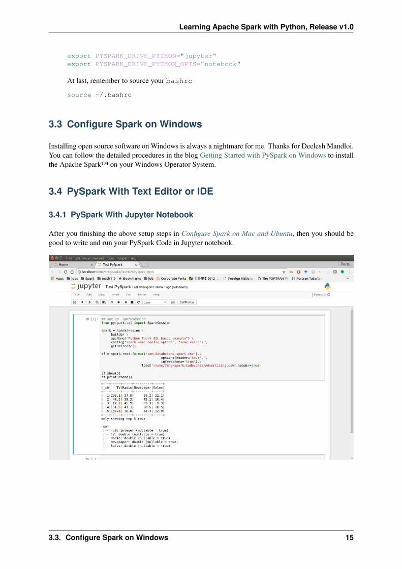
3.4.1 PySpark With Jupyter Notebook
After you finishing the above setup steps in Configure Spark on Mac and Ubuntu, then you should begood to write and run your PySpark Code in Jupyter notebook.
3.3. Configure Spark on Windows 15
Learning Apache Spark with Python, Release v1.0
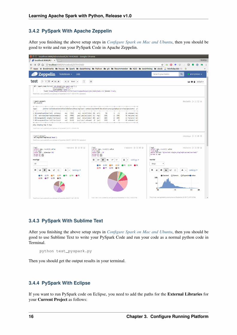
3.4.2 PySpark With Apache Zeppelin
After you finishing the above setup steps in Configure Spark on Mac and Ubuntu, then you should begood to write and run your PySpark Code in Apache Zeppelin.
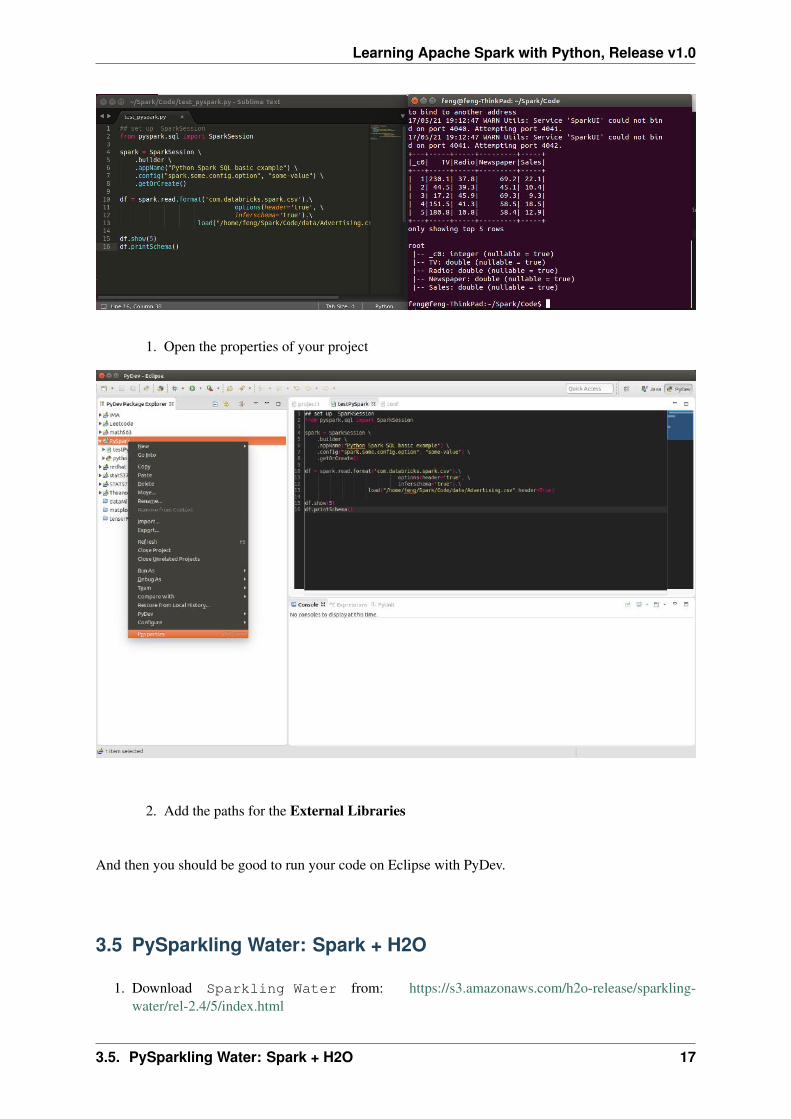
3.4.3 PySpark With Sublime Text
After you finishing the above setup steps in Configure Spark on Mac and Ubuntu, then you should begood to use Sublime Text to write your PySpark Code and run your code as a normal python code inTerminal.
python test_pyspark.py
Then you should get the output results in your terminal.
3.4.4 PySpark With Eclipse
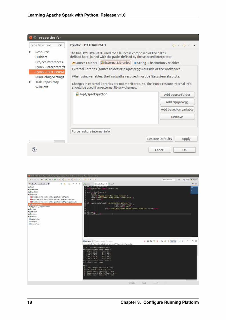
If you want to run PySpark code on Eclipse, you need to add the paths for the External Libraries foryour Current Project as follows:
16 Chapter 3. Configure Running Platform
Learning Apache Spark with Python, Release v1.0
1. Open the properties of your project
2. Add the paths for the External Libraries
And then you should be good to run your code on Eclipse with PyDev.
3.5 PySparkling Water: Spark + H2O
1. Download Sparkling Water from: https://s3.amazonaws.com/h2o-release/sparkling-water/rel-2.4/5/index.html
3.5. PySparkling Water: Spark + H2O 17
Learning Apache Spark with Python, Release v1.0
18 Chapter 3. Configure Running Platform
Learning Apache Spark with Python, Release v1.0
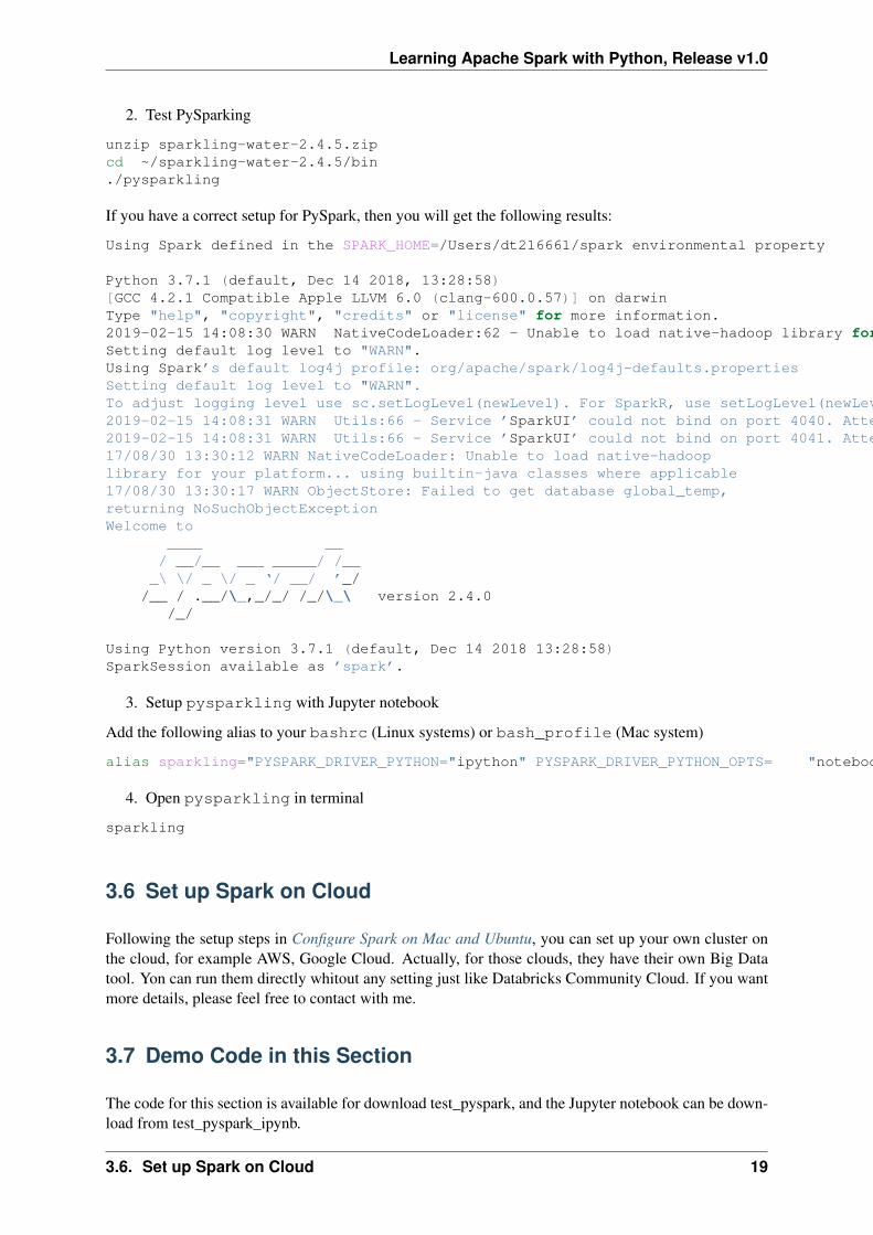
2. Test PySparking
unzip sparkling-water-2.4.5.zipcd ~/sparkling-water-2.4.5/bin./pysparkling
If you have a correct setup for PySpark, then you will get the following results:
Using Spark defined in the SPARK_HOME=/Users/dt216661/spark environmental property
Python 3.7.1 (default, Dec 14 2018, 13:28:58)[GCC 4.2.1 Compatible Apple LLVM 6.0 (clang-600.0.57)] on darwinType "help", "copyright", "credits" or "license" for more information.2019-02-15 14:08:30 WARN NativeCodeLoader:62 - Unable to load native-hadoop library for your platform... using builtin-java classes where applicableSetting default log level to "WARN".Using Spark’s default log4j profile: org/apache/spark/log4j-defaults.propertiesSetting default log level to "WARN".To adjust logging level use sc.setLogLevel(newLevel). For SparkR, use setLogLevel(newLevel).2019-02-15 14:08:31 WARN Utils:66 - Service ’SparkUI’ could not bind on port 4040. Attempting port 4041.2019-02-15 14:08:31 WARN Utils:66 - Service ’SparkUI’ could not bind on port 4041. Attempting port 4042.17/08/30 13:30:12 WARN NativeCodeLoader: Unable to load native-hadooplibrary for your platform... using builtin-java classes where applicable17/08/30 13:30:17 WARN ObjectStore: Failed to get database global_temp,returning NoSuchObjectExceptionWelcome to
____ __/ __/__ ___ _____/ /__
_\ \/ _ \/ _ ‘/ __/ ’_//__ / .__/\_,_/_/ /_/\_\ version 2.4.0
/_/
Using Python version 3.7.1 (default, Dec 14 2018 13:28:58)SparkSession available as ’spark’.
3. Setup pysparkling with Jupyter notebook
Add the following alias to your bashrc (Linux systems) or bash_profile (Mac system)
alias sparkling="PYSPARK_DRIVER_PYTHON="ipython" PYSPARK_DRIVER_PYTHON_OPTS= "notebook" /~/~/sparkling-water-2.4.5/bin/pysparkling"
4. Open pysparkling in terminal
sparkling
3.6 Set up Spark on Cloud
Following the setup steps in Configure Spark on Mac and Ubuntu, you can set up your own cluster onthe cloud, for example AWS, Google Cloud. Actually, for those clouds, they have their own Big Datatool. Yon can run them directly whitout any setting just like Databricks Community Cloud. If you wantmore details, please feel free to contact with me.
3.7 Demo Code in this Section
The code for this section is available for download test_pyspark, and the Jupyter notebook can be down-load from test_pyspark_ipynb.
3.6. Set up Spark on Cloud 19
Learning Apache Spark with Python, Release v1.0
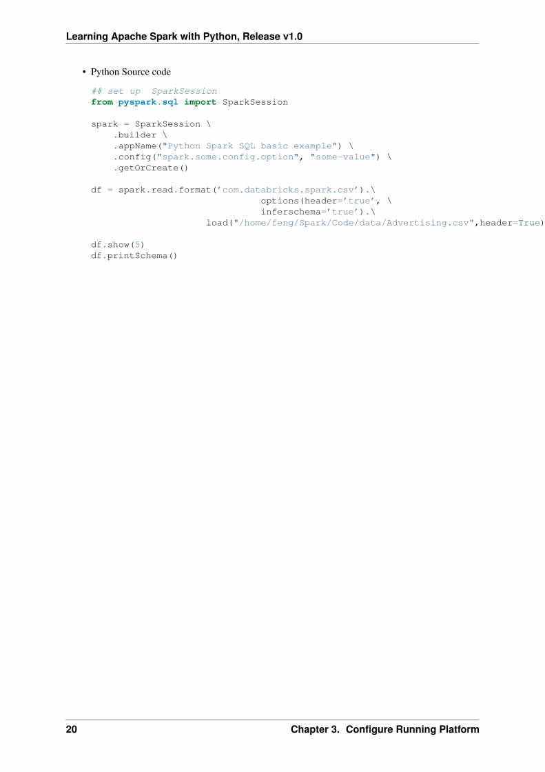
• Python Source code
## set up SparkSessionfrom pyspark.sql import SparkSession
spark = SparkSession \.builder \.appName("Python Spark SQL basic example") \.config("spark.some.config.option", "some-value") \.getOrCreate()
df = spark.read.format(’com.databricks.spark.csv’).\options(header=’true’, \inferschema=’true’).\
load("/home/feng/Spark/Code/data/Advertising.csv",header=True)
df.show(5)df.printSchema()
20 Chapter 3. Configure Running Platform
CHAPTER
FOUR
AN INTRODUCTION TO APACHE SPARK
Chinese proverb
Know yourself and know your enemy, and you will never be defeated – idiom, from Sunzi’s Art ofWar
4.1 Core Concepts
Most of the following content comes from [Kirillov2016]. So the copyright belongs to Anton Kirillov.I will refer you to get more details from Apache Spark core concepts, architecture and internals.
Before diving deep into how Apache Spark works, lets understand the jargon of Apache Spark
• Job: A piece of code which reads some input from HDFS or local, performs some computationon the data and writes some output data.
• Stages: Jobs are divided into stages. Stages are classified as a Map or reduce stages (Its easier tounderstand if you have worked on Hadoop and want to correlate). Stages are divided based oncomputational boundaries, all computations (operators) cannot be Updated in a single Stage. Ithappens over many stages.
• Tasks: Each stage has some tasks, one task per partition. One task is executed on one partition ofdata on one executor (machine).
• DAG: DAG stands for Directed Acyclic Graph, in the present context its a DAG of operators.
• Executor: The process responsible for executing a task.
• Master: The machine on which the Driver program runs
• Slave: The machine on which the Executor program runs
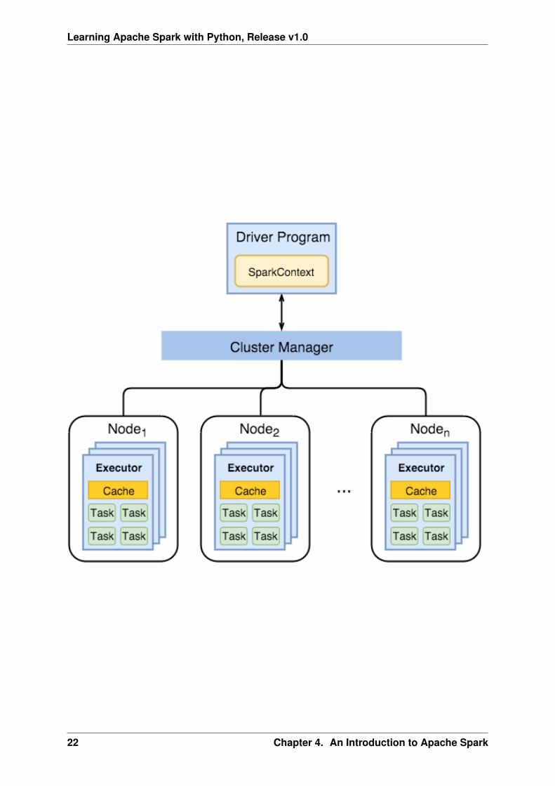
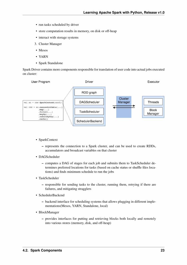
4.2 Spark Components
1. Spark Driver
• separate process to execute user applications
• creates SparkContext to schedule jobs execution and negotiate with cluster manager
2. Executors
21
Learning Apache Spark with Python, Release v1.0
22 Chapter 4. An Introduction to Apache Spark
Learning Apache Spark with Python, Release v1.0
• run tasks scheduled by driver
• store computation results in memory, on disk or off-heap
• interact with storage systems
3. Cluster Manager
• Mesos
• YARN
• Spark Standalone
Spark Driver contains more components responsible for translation of user code into actual jobs executedon cluster:
• SparkContext
– represents the connection to a Spark cluster, and can be used to create RDDs,accumulators and broadcast variables on that cluster
• DAGScheduler
– computes a DAG of stages for each job and submits them to TaskScheduler de-termines preferred locations for tasks (based on cache status or shuffle files loca-tions) and finds minimum schedule to run the jobs
• TaskScheduler
– responsible for sending tasks to the cluster, running them, retrying if there arefailures, and mitigating stragglers
• SchedulerBackend
– backend interface for scheduling systems that allows plugging in different imple-mentations(Mesos, YARN, Standalone, local)
• BlockManager
– provides interfaces for putting and retrieving blocks both locally and remotelyinto various stores (memory, disk, and off-heap)
4.2. Spark Components 23
Learning Apache Spark with Python, Release v1.0
4.3 Architecture
4.4 How Spark Works?
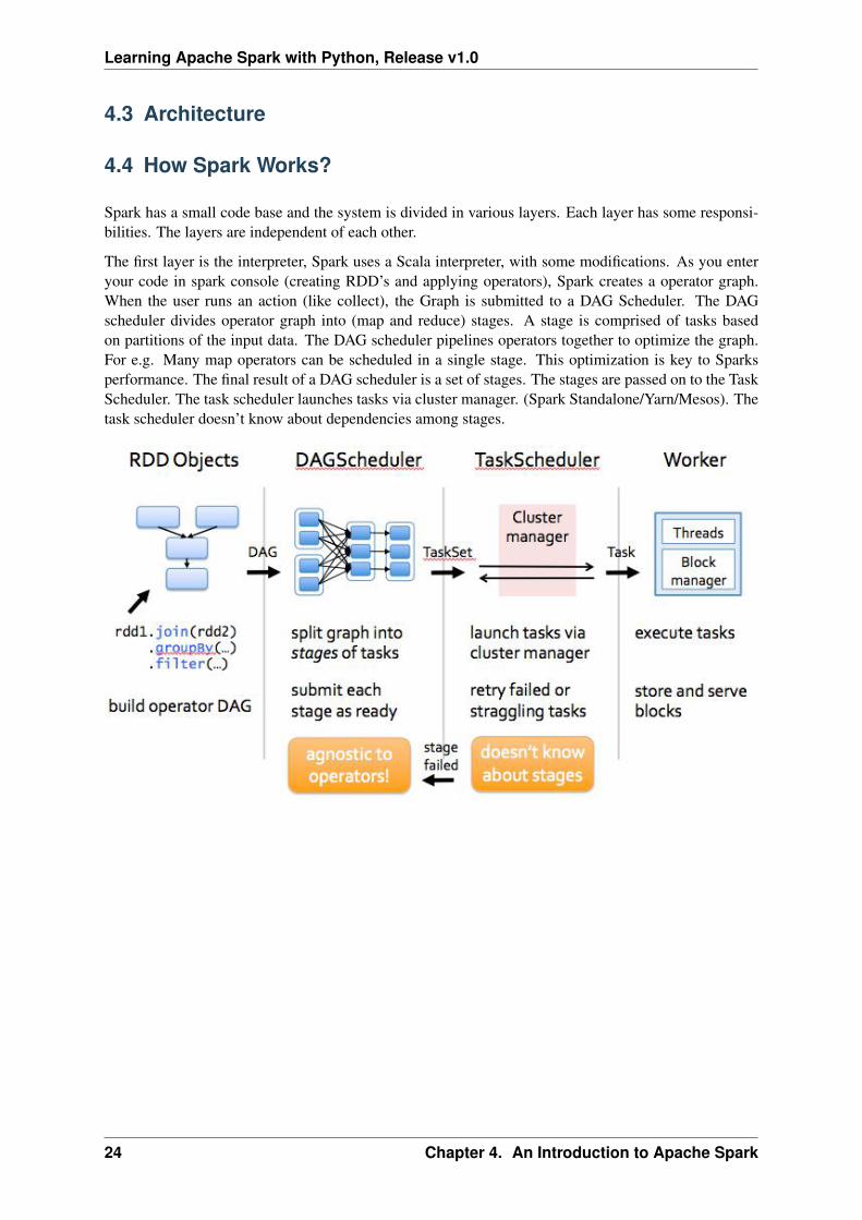
Spark has a small code base and the system is divided in various layers. Each layer has some responsi-bilities. The layers are independent of each other.
The first layer is the interpreter, Spark uses a Scala interpreter, with some modifications. As you enteryour code in spark console (creating RDD’s and applying operators), Spark creates a operator graph.When the user runs an action (like collect), the Graph is submitted to a DAG Scheduler. The DAGscheduler divides operator graph into (map and reduce) stages. A stage is comprised of tasks basedon partitions of the input data. The DAG scheduler pipelines operators together to optimize the graph.For e.g. Many map operators can be scheduled in a single stage. This optimization is key to Sparksperformance. The final result of a DAG scheduler is a set of stages. The stages are passed on to the TaskScheduler. The task scheduler launches tasks via cluster manager. (Spark Standalone/Yarn/Mesos). Thetask scheduler doesn’t know about dependencies among stages.
24 Chapter 4. An Introduction to Apache Spark
CHAPTER
FIVE
PROGRAMMING WITH RDDS
Chinese proverb
If you only know yourself, but not your opponent, you may win or may lose. If you know neitheryourself nor your enemy, you will always endanger yourself – idiom, from Sunzi’s Art of War
RDD represents Resilient Distributed Dataset. An RDD in Spark is simply an immutable distributedcollection of objects sets. Each RDD is split into multiple partitions (similar pattern with smaller sets),which may be computed on different nodes of the cluster.
5.1 Create RDD
Usually, there are two popular way to create the RDDs: loading an external dataset, or distributing a setof collection of objects. The following examples show some simplest ways to create RDDs by usingparallelize() fucntion which takes an already existing collection in your program and pass thesame to the Spark Context.
1. By using parallelize( ) fucntion
from pyspark.sql import SparkSession
spark = SparkSession \.builder \.appName("Python Spark create RDD example") \.config("spark.some.config.option", "some-value") \.getOrCreate()
df = spark.sparkContext.parallelize([(1, 2, 3, ’a b c’),(4, 5, 6, ’d e f’),(7, 8, 9, ’g h i’)]).toDF([’col1’, ’col2’, ’col3’,’col4’])
Then you will get the RDD data:
df.show()
+----+----+----+-----+|col1|col2|col3| col4|+----+----+----+-----+| 1| 2| 3|a b c|| 4| 5| 6|d e f|| 7| 8| 9|g h i|+----+----+----+-----+
25
Learning Apache Spark with Python, Release v1.0
from pyspark.sql import SparkSession
spark = SparkSession \.builder \.appName("Python Spark create RDD example") \.config("spark.some.config.option", "some-value") \.getOrCreate()
myData = spark.sparkContext.parallelize([(1,2), (3,4), (5,6), (7,8), (9,10)])
Then you will get the RDD data:
myData.collect()
[(1, 2), (3, 4), (5, 6), (7, 8), (9, 10)]
2. By using createDataFrame( ) function
from pyspark.sql import SparkSession
spark = SparkSession \.builder \.appName("Python Spark create RDD example") \.config("spark.some.config.option", "some-value") \.getOrCreate()
Employee = spark.createDataFrame([(’1’, ’Joe’, ’70000’, ’1’),(’2’, ’Henry’, ’80000’, ’2’),(’3’, ’Sam’, ’60000’, ’2’),(’4’, ’Max’, ’90000’, ’1’)],[’Id’, ’Name’, ’Sallary’,’DepartmentId’]
)
Then you will get the RDD data:
+---+-----+-------+------------+| Id| Name|Sallary|DepartmentId|+---+-----+-------+------------+| 1| Joe| 70000| 1|| 2|Henry| 80000| 2|| 3| Sam| 60000| 2|| 4| Max| 90000| 1|+---+-----+-------+------------+
3. By using read and load functions
1. Read dataset from .csv file
## set up SparkSessionfrom pyspark.sql import SparkSession
spark = SparkSession \.builder \.appName("Python Spark create RDD example") \.config("spark.some.config.option", "some-value") \.getOrCreate()
df = spark.read.format(’com.databricks.spark.csv’).\
26 Chapter 5. Programming with RDDs
Learning Apache Spark with Python, Release v1.0
options(header=’true’, \inferschema=’true’).\
load("/home/feng/Spark/Code/data/Advertising.csv",header=True)
df.show(5)df.printSchema()
Then you will get the RDD data:
+---+-----+-----+---------+-----+|_c0| TV|Radio|Newspaper|Sales|+---+-----+-----+---------+-----+| 1|230.1| 37.8| 69.2| 22.1|| 2| 44.5| 39.3| 45.1| 10.4|| 3| 17.2| 45.9| 69.3| 9.3|| 4|151.5| 41.3| 58.5| 18.5|| 5|180.8| 10.8| 58.4| 12.9|+---+-----+-----+---------+-----+only showing top 5 rows
root|-- _c0: integer (nullable = true)|-- TV: double (nullable = true)|-- Radio: double (nullable = true)|-- Newspaper: double (nullable = true)|-- Sales: double (nullable = true)
Once created, RDDs offer two types of operations: transformations and actions.
2. Read dataset from DataBase
## set up SparkSessionfrom pyspark.sql import SparkSession
spark = SparkSession \.builder \.appName("Python Spark create RDD example") \.config("spark.some.config.option", "some-value") \.getOrCreate()
## User informationuser = ’your_username’pw = ’your_password’
## Database informationtable_name = ’table_name’url = ’jdbc:postgresql://##.###.###.##:5432/dataset?user=’+user+’&password=’+pwproperties ={’driver’: ’org.postgresql.Driver’, ’password’: pw,’user’: user}
df = spark.read.jdbc(url=url, table=table_name, properties=properties)
df.show(5)df.printSchema()
Then you will get the RDD data:
+---+-----+-----+---------+-----+|_c0| TV|Radio|Newspaper|Sales|+---+-----+-----+---------+-----+
5.1. Create RDD 27
Learning Apache Spark with Python, Release v1.0
| 1|230.1| 37.8| 69.2| 22.1|| 2| 44.5| 39.3| 45.1| 10.4|| 3| 17.2| 45.9| 69.3| 9.3|| 4|151.5| 41.3| 58.5| 18.5|| 5|180.8| 10.8| 58.4| 12.9|+---+-----+-----+---------+-----+only showing top 5 rows
root|-- _c0: integer (nullable = true)|-- TV: double (nullable = true)|-- Radio: double (nullable = true)|-- Newspaper: double (nullable = true)|-- Sales: double (nullable = true)
Note:
Reading tables from Database needs the proper drive for the corresponding Database. Forexample, the above demo needs org.postgresql.Driver and you need to down-load it and put it in ‘‘jars‘‘ folder of your spark installation path. I downloadpostgresql-42.1.1.jar from the official website and put it in jars folder.
3. Read dataset from HDFS
from pyspark.conf import SparkConffrom pyspark.context import SparkContextfrom pyspark.sql import HiveContext
sc= SparkContext(’local’,’example’)hc = HiveContext(sc)tf1 = sc.textFile("hdfs://cdhstltest/user/data/demo.CSV")print(tf1.first())
hc.sql("use intg_cme_w")spf = hc.sql("SELECT * FROM spf LIMIT 100")print(spf.show(5))
5.2 Spark Operations
Warning: All the figures below are from Jeffrey Thompson. The interested reader is referred topyspark pictures
There are two main types of Spark operations: Transformations and Actions.
Note: Some people defined three types of operations: Transformations, Actions and Shuffles.
28 Chapter 5. Programming with RDDs
Learning Apache Spark with Python, Release v1.0
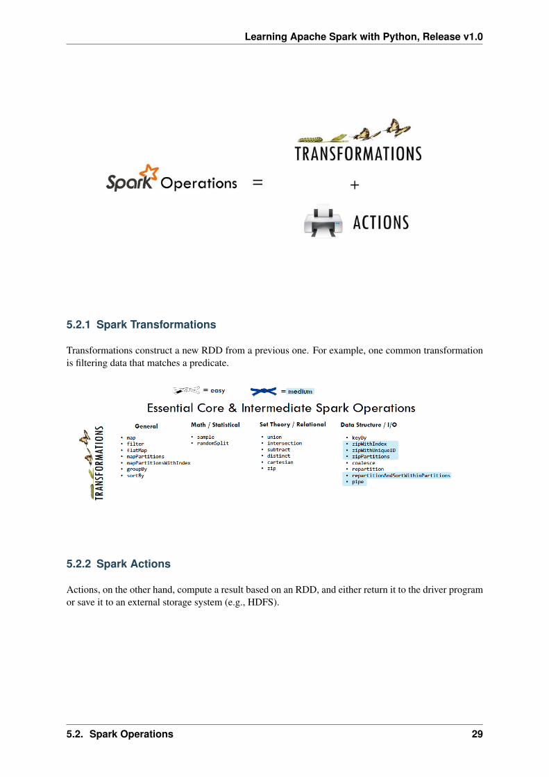
5.2.1 Spark Transformations
Transformations construct a new RDD from a previous one. For example, one common transformationis filtering data that matches a predicate.
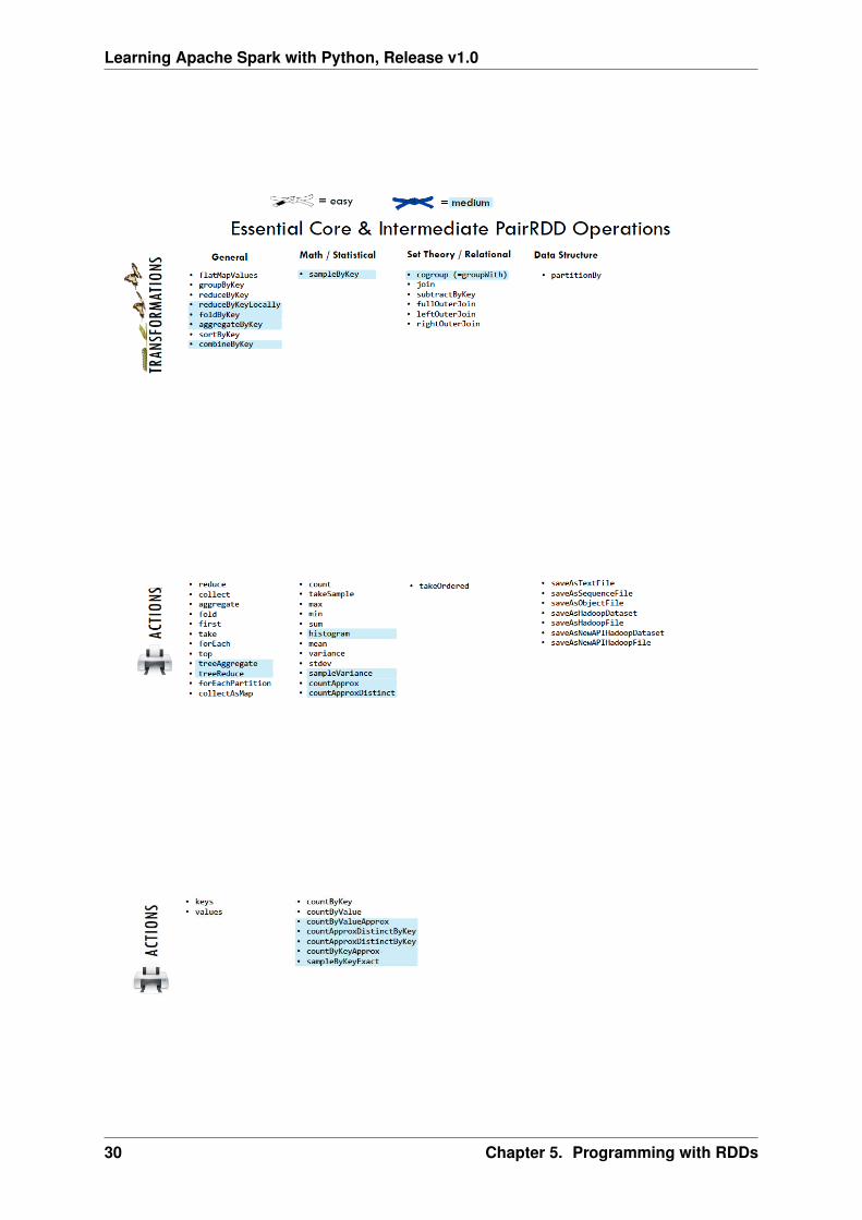
5.2.2 Spark Actions
Actions, on the other hand, compute a result based on an RDD, and either return it to the driver programor save it to an external storage system (e.g., HDFS).
5.2. Spark Operations 29
Learning Apache Spark with Python, Release v1.0
30 Chapter 5. Programming with RDDs
CHAPTER
SIX
STATISTICS PRELIMINARY
Chinese proverb
If you only know yourself, but not your opponent, you may win or may lose. If you know neitheryourself nor your enemy, you will always endanger yourself – idiom, from Sunzi’s Art of War
6.1 Notations
• m : the number of the samples
• n : the number of the features
• 𝑦𝑖 : i-th label
• 𝑦 = 1𝑚
∑︀𝑛𝑖=1 𝑦𝑖: the mean of 𝑦.
6.2 Measurement Formula
• Mean squared error
In statistics, the MSE (Mean Squared Error) of an estimator (of a procedure for estimating an unobservedquantity) measures the average of the squares of the errors or deviations—that is, the difference betweenthe estimator and what is estimated.
MSE =1
𝑚
𝑚∑︁𝑖=1
(𝑦𝑖 − 𝑦𝑖)2
• Root Mean squared error
RMSE =√
MSE =
⎯⎸⎸⎷ 1
𝑚
𝑚∑︁𝑖=1
(𝑦𝑖 − 𝑦𝑖)2
• Total sum of squares
In statistical data analysis the TSS (Total Sum of Squares) is a quantity that appears as part of a standardway of presenting results of such analyses. It is defined as being the sum, over all observations, of thesquared differences of each observation from the overall mean.
TSS =
𝑚∑︁𝑖=1
(𝑦𝑖 − 𝑦)2
31
Learning Apache Spark with Python, Release v1.0
• Residual Sum of Squares
RSS =1
𝑚
𝑚∑︁𝑖=1
(𝑦𝑖 − 𝑦𝑖)2
• Coefficient of determination 𝑅2
𝑅2 := 1 − RSSTSS
.
6.3 Statistical Tests
6.3.1 Correlational Test
• Pearson correlation: Tests for the strength of the association between two continuous variables.
• Spearman correlation: Tests for the strength of the association between two ordinal variables (doesnot rely on the assumption of normal distributed data).
• Chi-square: Tests for the strength of the association between two categorical variables.
6.3.2 Comparison of Means test
• Paired T-test: Tests for difference between two related variables.
• Independent T-test: Tests for difference between two independent variables.
• ANOVA: Tests the difference between group means after any other variance in the outcome vari-able is accounted for.
6.3.3 Non-parametric Test
• Wilcoxon rank-sum test: Tests for difference between two independent variables - takes into ac-count magnitude and direction of difference.
• Wilcoxon sign-rank test: Tests for difference between two related variables - takes into accountmagnitude and direction of difference.
• Sign test: Tests if two related variables are different – ignores magnitude of change, only takesinto account direction.
32 Chapter 6. Statistics Preliminary
CHAPTER
SEVEN
DATA EXPLORATION
Chinese proverb
A journey of a thousand miles begins with a single step – idiom, from Laozi.
I wouldn’t say that understanding your dataset is the most difficult thing in data science, but it is reallyimportant and time-consuming. Data Exploration is about describing the data by means of statisticaland visualization techniques. We explore data in order to understand the features and bring importantfeatures to our models.
7.1 Univariate Analysis
In mathematics, univariate refers to an expression, equation, function or polynomial of only one variable.“Uni” means “one”, so in other words your data has only one variable. So you do not need to dealwith the causes or relationships in this step. Univariate analysis takes data, summarizes that variables(attributes) one by one and finds patterns in the data.
There are many ways that can describe patterns found in univariate data include central tendency (mean,mode and median) and dispersion: range, variance, maximum, minimum, quartiles (including the in-terquartile range), coefficient of variation and standard deviation. You also have several options for vi-sualizing and describing data with univariate data. Such as frequency Distribution Tables,bar Charts, histograms, frequency Polygons, pie Charts.
The variable could be either categorical or numerical, I will demostrate the different statistical andvisulization techniques to investigate each type of the variable.
• The Jupyter notebook can be download from Data Exploration.
• The data can be downloaf from German Credit.
7.1.1 Numerical Variables
• Describe
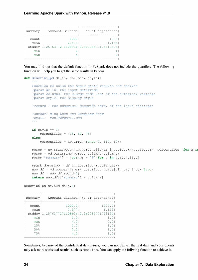
The desctibe function in pandas and spark will give us most of the statistical results, such asmin, median, max, quartiles and standard deviation. With the help of the user definedfunction, you can get even more statistical results.
# selected varables for the demonstrationnum_cols = [’Account Balance’,’No of dependents’]df.select(num_cols).describe().show()
33
Learning Apache Spark with Python, Release v1.0
+-------+------------------+-------------------+|summary| Account Balance| No of dependents|+-------+------------------+-------------------+| count| 1000| 1000|| mean| 2.577| 1.155|| stddev|1.2576377271108936|0.36208577175319395|| min| 1| 1|| max| 4| 2|+-------+------------------+-------------------+
You may find out that the default function in PySpark does not include the quartiles. The followingfunction will help you to get the same results in Pandas
def describe_pd(df_in, columns, style):’’’Function to union the basic stats results and deciles:param df_in: the input dataframe:param columns: the cloumn name list of the numerical variable:param style: the display style
:return : the numerical describe info. of the input dataframe
:author: MIng Chen and Wenqiang Feng:email: [email protected]’’’
if style == 1:percentiles = [25, 50, 75]
else:percentiles = np.array(range(0, 110, 10))
percs = np.transpose([np.percentile(df_in.select(x).collect(), percentiles) for x in columns])percs = pd.DataFrame(percs, columns=columns)percs[’summary’] = [str(p) + ’%’ for p in percentiles]
spark_describe = df_in.describe().toPandas()new_df = pd.concat([spark_describe, percs],ignore_index=True)new_df = new_df.round(2)return new_df[[’summary’] + columns]
describe_pd(df,num_cols,1)
+-------+------------------+-----------------+|summary| Account Balance| No of dependents|+-------+------------------+-----------------+| count| 1000.0| 1000.0|| mean| 2.577| 1.155|| stddev|1.2576377271108936|0.362085771753194|| min| 1.0| 1.0|| max| 4.0| 2.0|| 25%| 1.0| 1.0|| 50%| 2.0| 1.0|| 75%| 4.0| 1.0|+-------+------------------+-----------------+
Sometimes, because of the confidential data issues, you can not deliver the real data and your clientsmay ask more statistical results, such as deciles. You can apply the follwing function to achieve it.
34 Chapter 7. Data Exploration
Learning Apache Spark with Python, Release v1.0
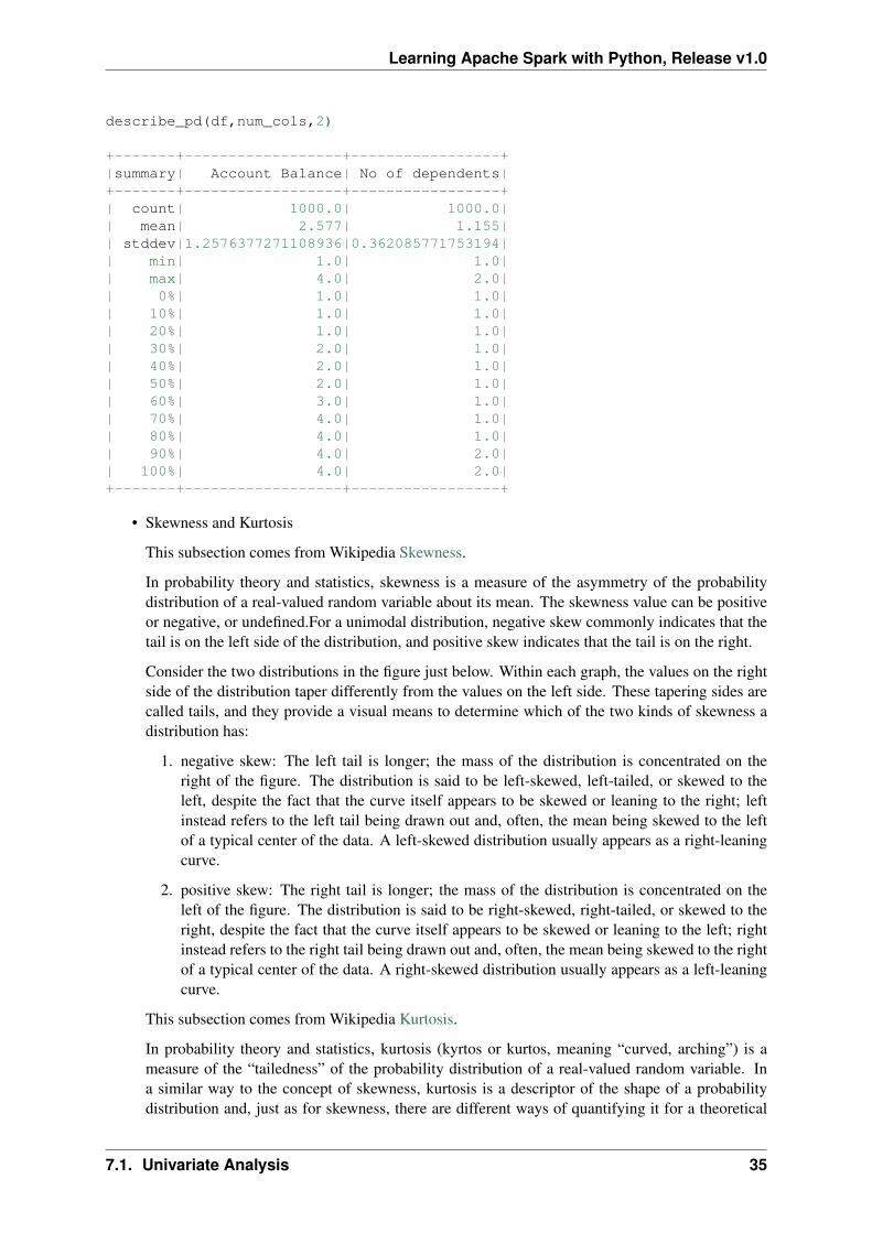
describe_pd(df,num_cols,2)
+-------+------------------+-----------------+|summary| Account Balance| No of dependents|+-------+------------------+-----------------+| count| 1000.0| 1000.0|| mean| 2.577| 1.155|| stddev|1.2576377271108936|0.362085771753194|| min| 1.0| 1.0|| max| 4.0| 2.0|| 0%| 1.0| 1.0|| 10%| 1.0| 1.0|| 20%| 1.0| 1.0|| 30%| 2.0| 1.0|| 40%| 2.0| 1.0|| 50%| 2.0| 1.0|| 60%| 3.0| 1.0|| 70%| 4.0| 1.0|| 80%| 4.0| 1.0|| 90%| 4.0| 2.0|| 100%| 4.0| 2.0|+-------+------------------+-----------------+
• Skewness and Kurtosis
This subsection comes from Wikipedia Skewness.
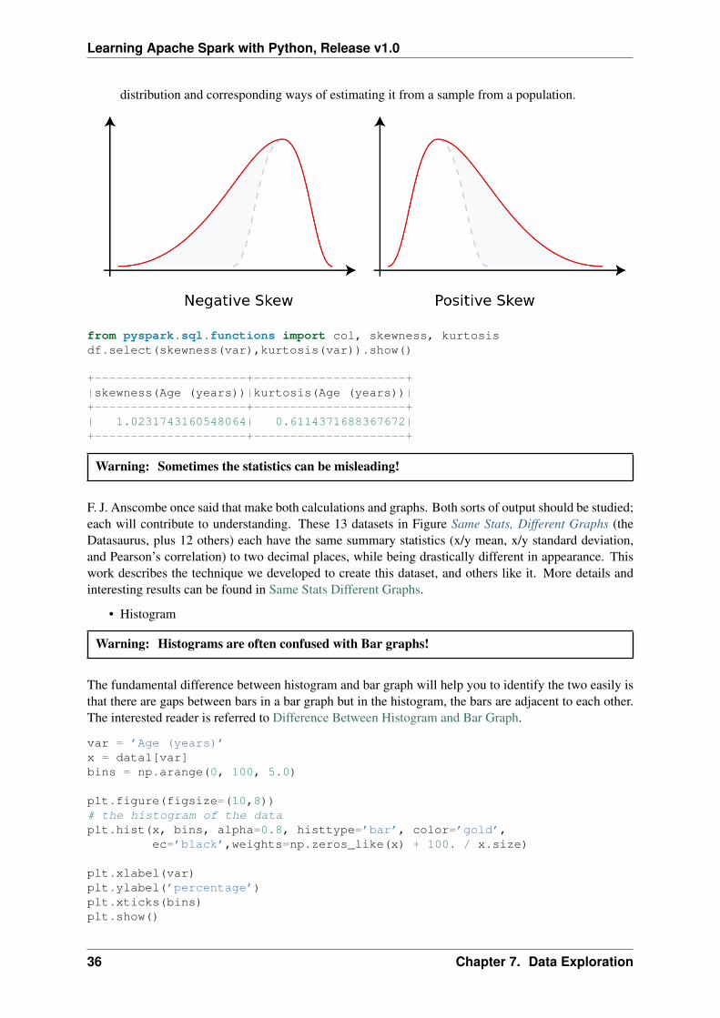
In probability theory and statistics, skewness is a measure of the asymmetry of the probabilitydistribution of a real-valued random variable about its mean. The skewness value can be positiveor negative, or undefined.For a unimodal distribution, negative skew commonly indicates that thetail is on the left side of the distribution, and positive skew indicates that the tail is on the right.
Consider the two distributions in the figure just below. Within each graph, the values on the rightside of the distribution taper differently from the values on the left side. These tapering sides arecalled tails, and they provide a visual means to determine which of the two kinds of skewness adistribution has:
1. negative skew: The left tail is longer; the mass of the distribution is concentrated on theright of the figure. The distribution is said to be left-skewed, left-tailed, or skewed to theleft, despite the fact that the curve itself appears to be skewed or leaning to the right; leftinstead refers to the left tail being drawn out and, often, the mean being skewed to the leftof a typical center of the data. A left-skewed distribution usually appears as a right-leaningcurve.
2. positive skew: The right tail is longer; the mass of the distribution is concentrated on theleft of the figure. The distribution is said to be right-skewed, right-tailed, or skewed to theright, despite the fact that the curve itself appears to be skewed or leaning to the left; rightinstead refers to the right tail being drawn out and, often, the mean being skewed to the rightof a typical center of the data. A right-skewed distribution usually appears as a left-leaningcurve.
This subsection comes from Wikipedia Kurtosis.
In probability theory and statistics, kurtosis (kyrtos or kurtos, meaning “curved, arching”) is ameasure of the “tailedness” of the probability distribution of a real-valued random variable. Ina similar way to the concept of skewness, kurtosis is a descriptor of the shape of a probabilitydistribution and, just as for skewness, there are different ways of quantifying it for a theoretical
7.1. Univariate Analysis 35
Learning Apache Spark with Python, Release v1.0
distribution and corresponding ways of estimating it from a sample from a population.
from pyspark.sql.functions import col, skewness, kurtosisdf.select(skewness(var),kurtosis(var)).show()
+---------------------+---------------------+|skewness(Age (years))|kurtosis(Age (years))|+---------------------+---------------------+| 1.0231743160548064| 0.6114371688367672|+---------------------+---------------------+
Warning: Sometimes the statistics can be misleading!
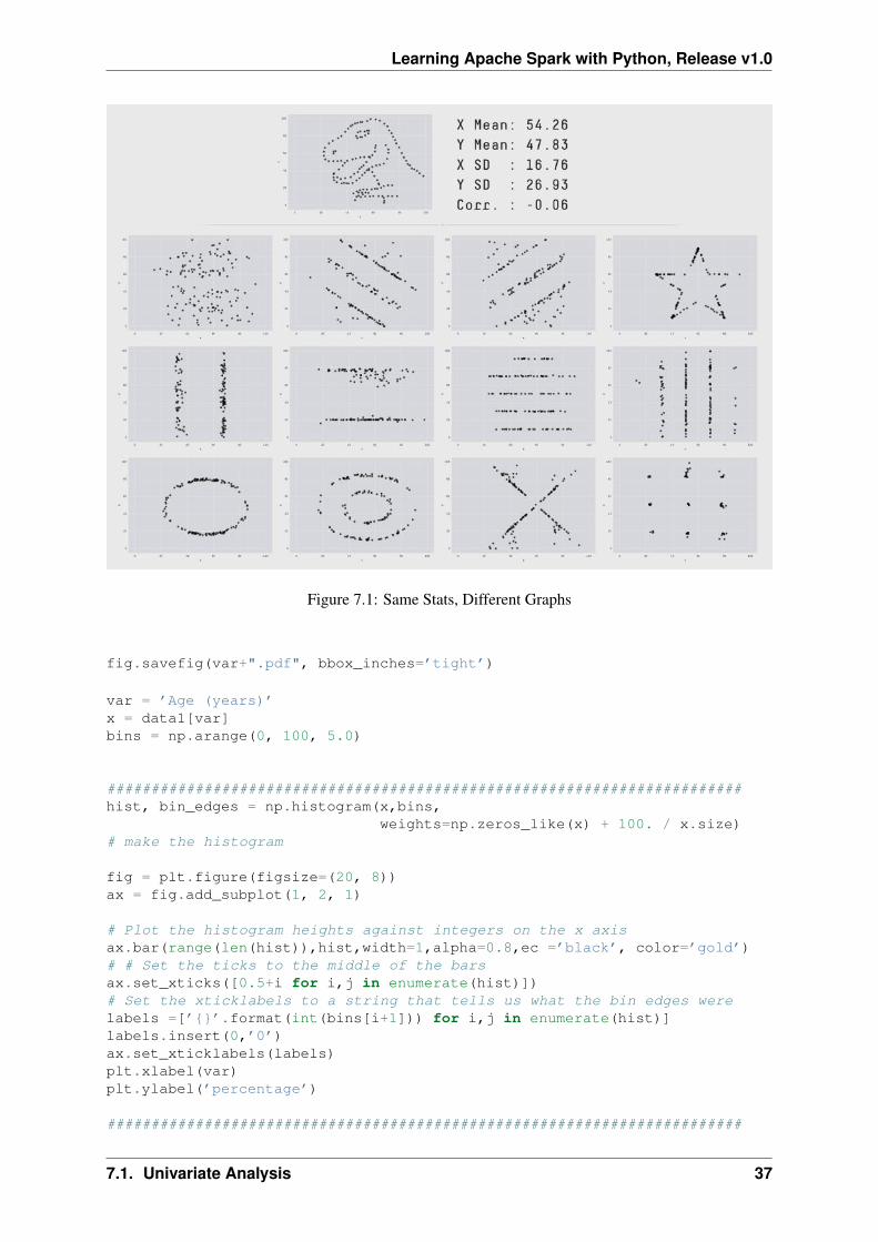
F. J. Anscombe once said that make both calculations and graphs. Both sorts of output should be studied;each will contribute to understanding. These 13 datasets in Figure Same Stats, Different Graphs (theDatasaurus, plus 12 others) each have the same summary statistics (x/y mean, x/y standard deviation,and Pearson’s correlation) to two decimal places, while being drastically different in appearance. Thiswork describes the technique we developed to create this dataset, and others like it. More details andinteresting results can be found in Same Stats Different Graphs.
• Histogram
Warning: Histograms are often confused with Bar graphs!
The fundamental difference between histogram and bar graph will help you to identify the two easily isthat there are gaps between bars in a bar graph but in the histogram, the bars are adjacent to each other.The interested reader is referred to Difference Between Histogram and Bar Graph.
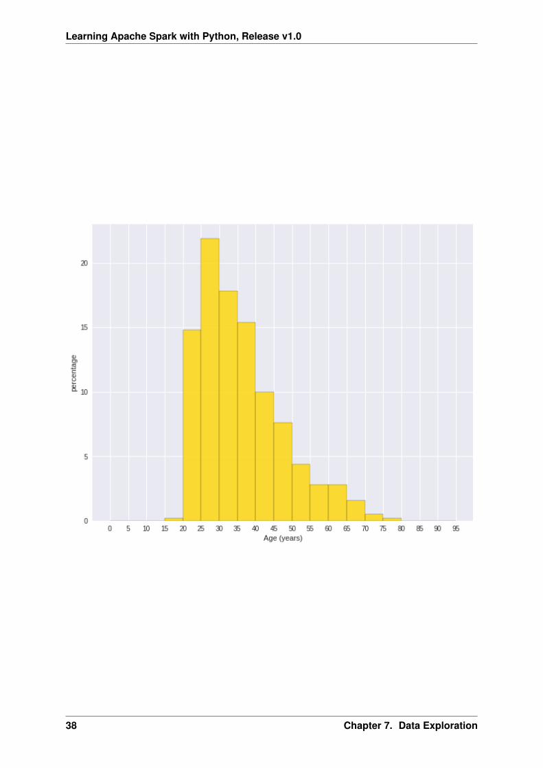
var = ’Age (years)’x = data1[var]bins = np.arange(0, 100, 5.0)
plt.figure(figsize=(10,8))# the histogram of the dataplt.hist(x, bins, alpha=0.8, histtype=’bar’, color=’gold’,
ec=’black’,weights=np.zeros_like(x) + 100. / x.size)
plt.xlabel(var)plt.ylabel(’percentage’)plt.xticks(bins)plt.show()
36 Chapter 7. Data Exploration
Learning Apache Spark with Python, Release v1.0
Figure 7.1: Same Stats, Different Graphs
fig.savefig(var+".pdf", bbox_inches=’tight’)
var = ’Age (years)’x = data1[var]bins = np.arange(0, 100, 5.0)
########################################################################hist, bin_edges = np.histogram(x,bins,
weights=np.zeros_like(x) + 100. / x.size)# make the histogram
fig = plt.figure(figsize=(20, 8))ax = fig.add_subplot(1, 2, 1)
# Plot the histogram heights against integers on the x axisax.bar(range(len(hist)),hist,width=1,alpha=0.8,ec =’black’, color=’gold’)# # Set the ticks to the middle of the barsax.set_xticks([0.5+i for i,j in enumerate(hist)])# Set the xticklabels to a string that tells us what the bin edges werelabels =[’{}’.format(int(bins[i+1])) for i,j in enumerate(hist)]labels.insert(0,’0’)ax.set_xticklabels(labels)plt.xlabel(var)plt.ylabel(’percentage’)
########################################################################
7.1. Univariate Analysis 37
Learning Apache Spark with Python, Release v1.0
38 Chapter 7. Data Exploration
Learning Apache Spark with Python, Release v1.0
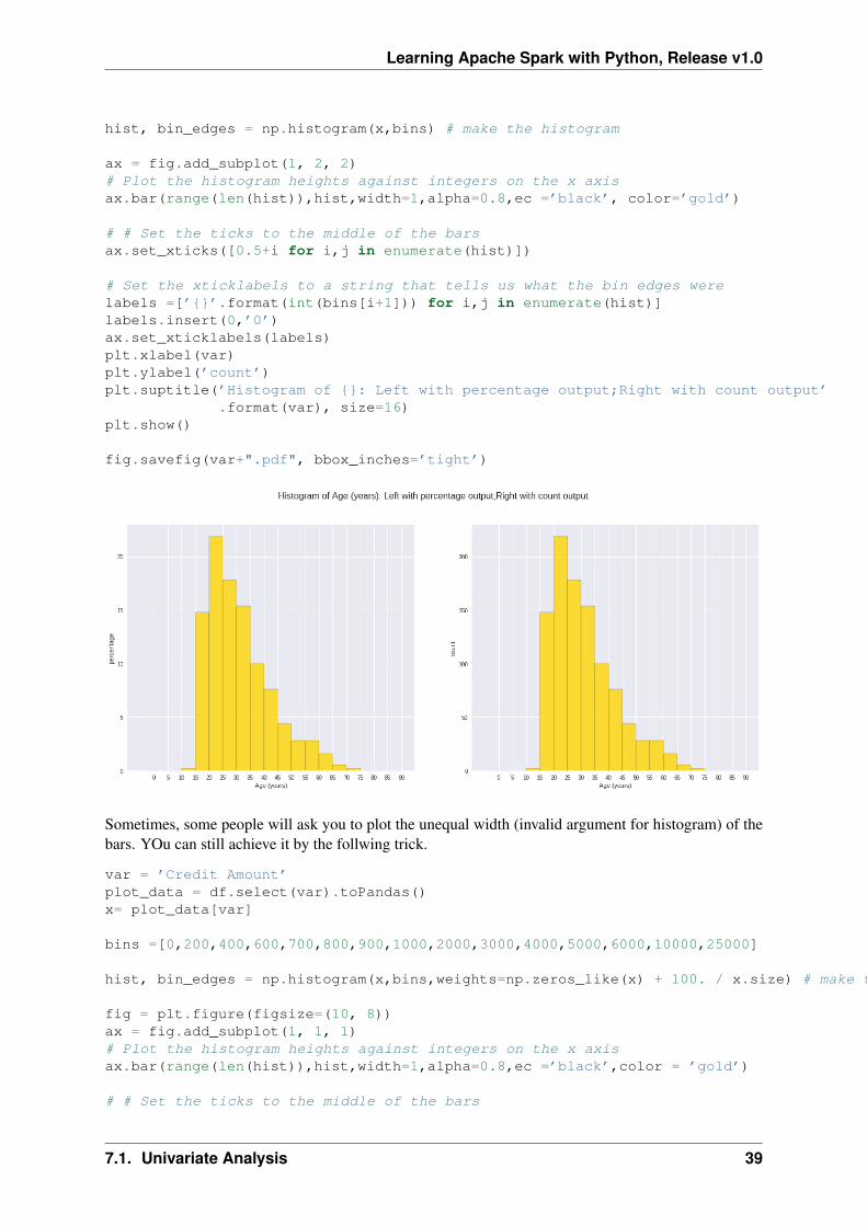
hist, bin_edges = np.histogram(x,bins) # make the histogram
ax = fig.add_subplot(1, 2, 2)# Plot the histogram heights against integers on the x axisax.bar(range(len(hist)),hist,width=1,alpha=0.8,ec =’black’, color=’gold’)
# # Set the ticks to the middle of the barsax.set_xticks([0.5+i for i,j in enumerate(hist)])
# Set the xticklabels to a string that tells us what the bin edges werelabels =[’{}’.format(int(bins[i+1])) for i,j in enumerate(hist)]labels.insert(0,’0’)ax.set_xticklabels(labels)plt.xlabel(var)plt.ylabel(’count’)plt.suptitle(’Histogram of {}: Left with percentage output;Right with count output’
.format(var), size=16)plt.show()
fig.savefig(var+".pdf", bbox_inches=’tight’)
Sometimes, some people will ask you to plot the unequal width (invalid argument for histogram) of thebars. YOu can still achieve it by the follwing trick.
var = ’Credit Amount’plot_data = df.select(var).toPandas()x= plot_data[var]
bins =[0,200,400,600,700,800,900,1000,2000,3000,4000,5000,6000,10000,25000]
hist, bin_edges = np.histogram(x,bins,weights=np.zeros_like(x) + 100. / x.size) # make the histogram
fig = plt.figure(figsize=(10, 8))ax = fig.add_subplot(1, 1, 1)# Plot the histogram heights against integers on the x axisax.bar(range(len(hist)),hist,width=1,alpha=0.8,ec =’black’,color = ’gold’)
# # Set the ticks to the middle of the bars
7.1. Univariate Analysis 39
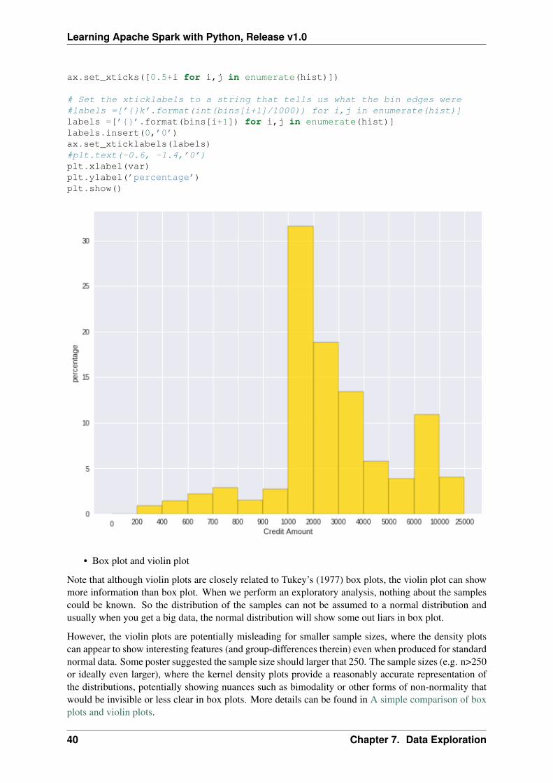
Learning Apache Spark with Python, Release v1.0
ax.set_xticks([0.5+i for i,j in enumerate(hist)])
# Set the xticklabels to a string that tells us what the bin edges were#labels =[’{}k’.format(int(bins[i+1]/1000)) for i,j in enumerate(hist)]labels =[’{}’.format(bins[i+1]) for i,j in enumerate(hist)]labels.insert(0,’0’)ax.set_xticklabels(labels)#plt.text(-0.6, -1.4,’0’)plt.xlabel(var)plt.ylabel(’percentage’)plt.show()
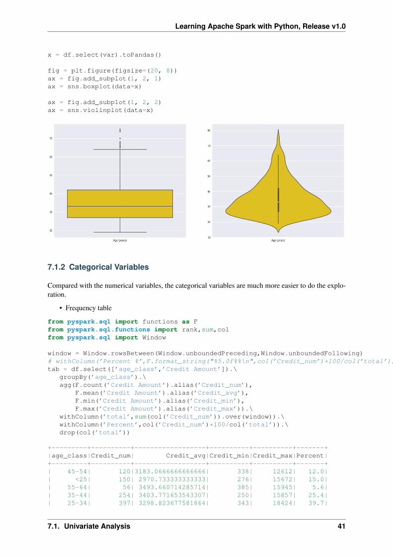
• Box plot and violin plot
Note that although violin plots are closely related to Tukey’s (1977) box plots, the violin plot can showmore information than box plot. When we perform an exploratory analysis, nothing about the samplescould be known. So the distribution of the samples can not be assumed to a normal distribution andusually when you get a big data, the normal distribution will show some out liars in box plot.
However, the violin plots are potentially misleading for smaller sample sizes, where the density plotscan appear to show interesting features (and group-differences therein) even when produced for standardnormal data. Some poster suggested the sample size should larger that 250. The sample sizes (e.g. n>250or ideally even larger), where the kernel density plots provide a reasonably accurate representation ofthe distributions, potentially showing nuances such as bimodality or other forms of non-normality thatwould be invisible or less clear in box plots. More details can be found in A simple comparison of boxplots and violin plots.
40 Chapter 7. Data Exploration
Learning Apache Spark with Python, Release v1.0
x = df.select(var).toPandas()
fig = plt.figure(figsize=(20, 8))ax = fig.add_subplot(1, 2, 1)ax = sns.boxplot(data=x)
ax = fig.add_subplot(1, 2, 2)ax = sns.violinplot(data=x)
7.1.2 Categorical Variables
Compared with the numerical variables, the categorical variables are much more easier to do the explo-ration.
• Frequency table
from pyspark.sql import functions as Ffrom pyspark.sql.functions import rank,sum,colfrom pyspark.sql import Window
window = Window.rowsBetween(Window.unboundedPreceding,Window.unboundedFollowing)# withColumn(’Percent %’,F.format_string("%5.0f%%\n",col(’Credit_num’)*100/col(’total’))).\tab = df.select([’age_class’,’Credit Amount’]).\
groupBy(’age_class’).\agg(F.count(’Credit Amount’).alias(’Credit_num’),
F.mean(’Credit Amount’).alias(’Credit_avg’),F.min(’Credit Amount’).alias(’Credit_min’),F.max(’Credit Amount’).alias(’Credit_max’)).\
withColumn(’total’,sum(col(’Credit_num’)).over(window)).\withColumn(’Percent’,col(’Credit_num’)*100/col(’total’)).\drop(col(’total’))
+---------+----------+------------------+----------+----------+-------+|age_class|Credit_num| Credit_avg|Credit_min|Credit_max|Percent|+---------+----------+------------------+----------+----------+-------+| 45-54| 120|3183.0666666666666| 338| 12612| 12.0|| <25| 150| 2970.733333333333| 276| 15672| 15.0|| 55-64| 56| 3493.660714285714| 385| 15945| 5.6|| 35-44| 254| 3403.771653543307| 250| 15857| 25.4|| 25-34| 397| 3298.823677581864| 343| 18424| 39.7|
7.1. Univariate Analysis 41
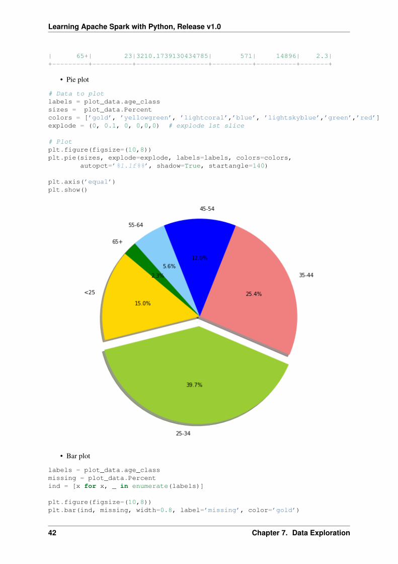
Learning Apache Spark with Python, Release v1.0
| 65+| 23|3210.1739130434785| 571| 14896| 2.3|+---------+----------+------------------+----------+----------+-------+
• Pie plot
# Data to plotlabels = plot_data.age_classsizes = plot_data.Percentcolors = [’gold’, ’yellowgreen’, ’lightcoral’,’blue’, ’lightskyblue’,’green’,’red’]explode = (0, 0.1, 0, 0,0,0) # explode 1st slice
# Plotplt.figure(figsize=(10,8))plt.pie(sizes, explode=explode, labels=labels, colors=colors,
autopct=’%1.1f%%’, shadow=True, startangle=140)
plt.axis(’equal’)plt.show()
• Bar plot
labels = plot_data.age_classmissing = plot_data.Percentind = [x for x, _ in enumerate(labels)]
plt.figure(figsize=(10,8))plt.bar(ind, missing, width=0.8, label=’missing’, color=’gold’)
42 Chapter 7. Data Exploration
Learning Apache Spark with Python, Release v1.0
plt.xticks(ind, labels)plt.ylabel("percentage")
plt.show()
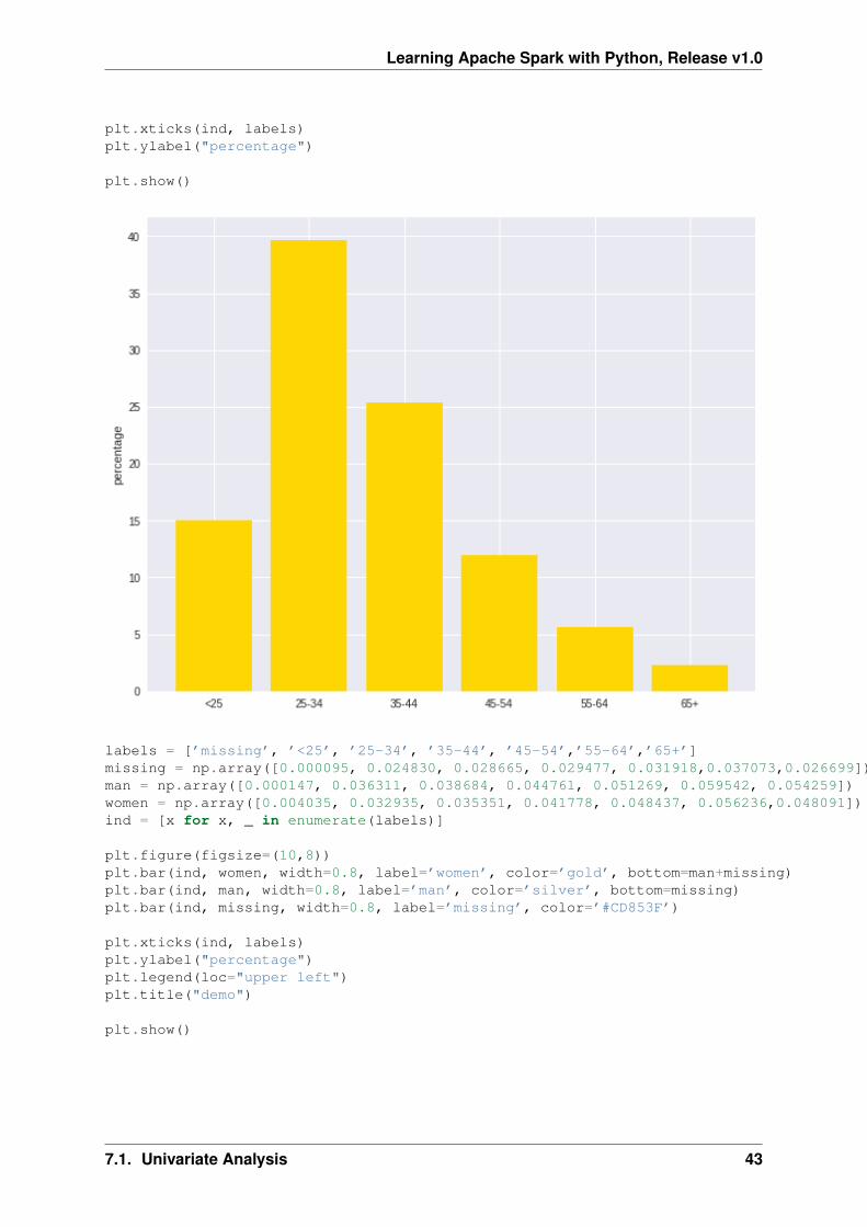
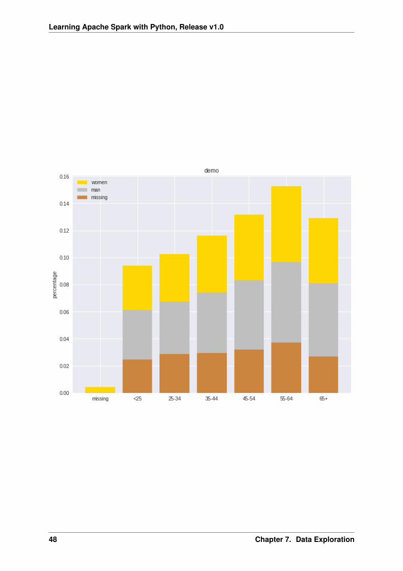
labels = [’missing’, ’<25’, ’25-34’, ’35-44’, ’45-54’,’55-64’,’65+’]missing = np.array([0.000095, 0.024830, 0.028665, 0.029477, 0.031918,0.037073,0.026699])man = np.array([0.000147, 0.036311, 0.038684, 0.044761, 0.051269, 0.059542, 0.054259])women = np.array([0.004035, 0.032935, 0.035351, 0.041778, 0.048437, 0.056236,0.048091])ind = [x for x, _ in enumerate(labels)]
plt.figure(figsize=(10,8))plt.bar(ind, women, width=0.8, label=’women’, color=’gold’, bottom=man+missing)plt.bar(ind, man, width=0.8, label=’man’, color=’silver’, bottom=missing)plt.bar(ind, missing, width=0.8, label=’missing’, color=’#CD853F’)
plt.xticks(ind, labels)plt.ylabel("percentage")plt.legend(loc="upper left")plt.title("demo")
plt.show()
7.1. Univariate Analysis 43

Learning Apache Spark with Python, Release v1.0
44 Chapter 7. Data Exploration
Learning Apache Spark with Python, Release v1.0
7.2 Multivariate Analysis
In this section, I will only demostrate the bivariate analysis. Since the multivariate analysis is the gener-ation of the bivariate.
7.2.1 Numerical V.S. Numerical
• Correlation matrix
from pyspark.mllib.stat import Statisticsimport pandas as pd
corr_data = df.select(num_cols)
col_names = corr_data.columnsfeatures = corr_data.rdd.map(lambda row: row[0:])corr_mat=Statistics.corr(features, method="pearson")corr_df = pd.DataFrame(corr_mat)corr_df.index, corr_df.columns = col_names, col_names
print(corr_df.to_string())
+--------------------+--------------------+| Account Balance| No of dependents|+--------------------+--------------------+| 1.0|-0.01414542650320914||-0.01414542650320914| 1.0|+--------------------+--------------------+
• Scatter Plot
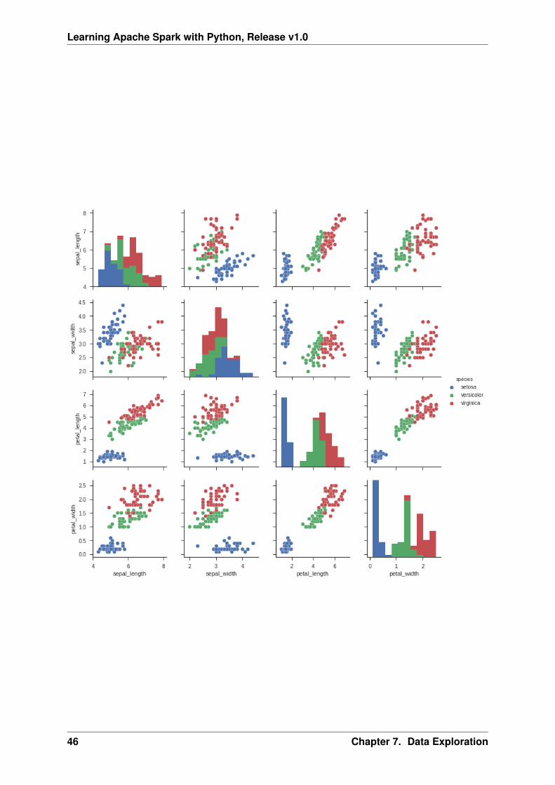
import seaborn as snssns.set(style="ticks")
df = sns.load_dataset("iris")sns.pairplot(df, hue="species")plt.show()
7.2.2 Categorical V.S. Categorical
• Pearson’s Chi-squared test
Warning: pyspark.ml.stat is only available in Spark 2.4.0.
from pyspark.ml.linalg import Vectorsfrom pyspark.ml.stat import ChiSquareTest
data = [(0.0, Vectors.dense(0.5, 10.0)),(0.0, Vectors.dense(1.5, 20.0)),(1.0, Vectors.dense(1.5, 30.0)),(0.0, Vectors.dense(3.5, 30.0)),(0.0, Vectors.dense(3.5, 40.0)),(1.0, Vectors.dense(3.5, 40.0))]
df = spark.createDataFrame(data, ["label", "features"])
7.2. Multivariate Analysis 45
Learning Apache Spark with Python, Release v1.0
46 Chapter 7. Data Exploration
Learning Apache Spark with Python, Release v1.0
r = ChiSquareTest.test(df, "features", "label").head()print("pValues: " + str(r.pValues))print("degreesOfFreedom: " + str(r.degreesOfFreedom))print("statistics: " + str(r.statistics))
pValues: [0.687289278791,0.682270330336]degreesOfFreedom: [2, 3]statistics: [0.75,1.5]
• Cross table
df.stat.crosstab("age_class", "Occupation").show()
+--------------------+---+---+---+---+|age_class_Occupation| 1| 2| 3| 4|+--------------------+---+---+---+---+| <25| 4| 34|108| 4|| 55-64| 1| 15| 31| 9|| 25-34| 7| 61|269| 60|| 35-44| 4| 58|143| 49|| 65+| 5| 3| 6| 9|| 45-54| 1| 29| 73| 17|+--------------------+---+---+---+---+
• Stacked plot
labels = [’missing’, ’<25’, ’25-34’, ’35-44’, ’45-54’,’55-64’,’65+’]missing = np.array([0.000095, 0.024830, 0.028665, 0.029477, 0.031918,0.037073,0.026699])man = np.array([0.000147, 0.036311, 0.038684, 0.044761, 0.051269, 0.059542, 0.054259])women = np.array([0.004035, 0.032935, 0.035351, 0.041778, 0.048437, 0.056236,0.048091])ind = [x for x, _ in enumerate(labels)]
plt.figure(figsize=(10,8))plt.bar(ind, women, width=0.8, label=’women’, color=’gold’, bottom=man+missing)plt.bar(ind, man, width=0.8, label=’man’, color=’silver’, bottom=missing)plt.bar(ind, missing, width=0.8, label=’missing’, color=’#CD853F’)
plt.xticks(ind, labels)plt.ylabel("percentage")plt.legend(loc="upper left")plt.title("demo")
plt.show()
7.2.3 Numerical V.S. Categorical
7.2. Multivariate Analysis 47
Learning Apache Spark with Python, Release v1.0
48 Chapter 7. Data Exploration
CHAPTER
EIGHT
REGRESSION
Chinese proverb
A journey of a thousand miles begins with a single step. – old Chinese proverb
In statistical modeling, regression analysis focuses on investigating the relationship between a dependentvariable and one or more independent variables. Wikipedia Regression analysis
In data mining, Regression is a model to represent the relationship between the value of lable ( or target,it is numerical variable) and on one or more features (or predictors they can be numerical and categoricalvariables).
8.1 Linear Regression
8.1.1 Introduction
Given that a data set {𝑥𝑖1, . . . , 𝑥𝑖𝑛, 𝑦𝑖}𝑚𝑖=1 which contains n features (variables) and m samples (datapoints), in simple linear regression model for modeling 𝑚 data points with one independent variable:𝑥𝑖1, the formula is given by:
𝑦𝑖 = 𝛽0 + 𝛽1𝑥𝑖1,where, 𝑖 = 1, · · ·𝑚.
In matrix notation, the data set is written as X = [X1, · · · ,X𝑛] with X𝑖 = {𝑥·𝑖}𝑛𝑖=1, y = {𝑦𝑖}𝑚𝑖=1 and𝛽⊤ = {𝛽𝑖}𝑚𝑖=1. Then the normal equations are written as
y = X𝛽.
8.1.2 How to solve it?
1. Direct Methods (For more information please refer to my Prelim Notes for Numerical Analysis)
• For squared or rectangular matrices
– Singular Value Decomposition
– Gram-Schmidt orthogonalization
– QR Decomposition
49
Learning Apache Spark with Python, Release v1.0
• For squared matrices
– LU Decomposition
– Cholesky Decomposition
– Regular Splittings
2. Iterative Methods
• Stationary cases iterative method
– Jacobi Method
– Gauss-Seidel Method
– Richardson Method
– Successive Over Relaxation (SOR) Method
• Dynamic cases iterative method
– Chebyshev iterative Method
– Minimal residuals Method
– Minimal correction iterative method
– Steepest Descent Method
– Conjugate Gradients Method
8.1.3 Demo
• The Jupyter notebook can be download from Linear Regression which was implemented withoutusing Pipeline.
• The Jupyter notebook can be download from Linear Regression with Pipeline which was imple-mented with using Pipeline.
• I will only present the code with pipeline style in the following.
• For more details about the parameters, please visit Linear Regression API .
1. Set up spark context and SparkSession
from pyspark.sql import SparkSession
spark = SparkSession \.builder \.appName("Python Spark regression example") \.config("spark.some.config.option", "some-value") \.getOrCreate()
2. Load dataset
df = spark.read.format(’com.databricks.spark.csv’).\options(header=’true’, \inferschema=’true’).\
load("../data/Advertising.csv",header=True);
check the data set
50 Chapter 8. Regression
Learning Apache Spark with Python, Release v1.0
df.show(5,True)df.printSchema()
Then you will get
+-----+-----+---------+-----+| TV|Radio|Newspaper|Sales|+-----+-----+---------+-----+|230.1| 37.8| 69.2| 22.1|| 44.5| 39.3| 45.1| 10.4|| 17.2| 45.9| 69.3| 9.3||151.5| 41.3| 58.5| 18.5||180.8| 10.8| 58.4| 12.9|+-----+-----+---------+-----+only showing top 5 rows
root|-- TV: double (nullable = true)|-- Radio: double (nullable = true)|-- Newspaper: double (nullable = true)|-- Sales: double (nullable = true)
You can also get the Statistical resutls from the data frame (Unfortunately, it only works for numerical).
df.describe().show()
Then you will get
+-------+-----------------+------------------+------------------+------------------+|summary| TV| Radio| Newspaper| Sales|+-------+-----------------+------------------+------------------+------------------+| count| 200| 200| 200| 200|| mean| 147.0425|23.264000000000024|30.553999999999995|14.022500000000003|| stddev|85.85423631490805|14.846809176168728| 21.77862083852283| 5.217456565710477|| min| 0.7| 0.0| 0.3| 1.6|| max| 296.4| 49.6| 114.0| 27.0|+-------+-----------------+------------------+------------------+------------------+
3. Convert the data to dense vector (features and label)
from pyspark.sql import Rowfrom pyspark.ml.linalg import Vectors
# I provide two ways to build the features and labels
# method 1 (good for small feature):#def transData(row):# return Row(label=row["Sales"],# features=Vectors.dense([row["TV"],# row["Radio"],# row["Newspaper"]]))
# Method 2 (good for large features):def transData(data):return data.rdd.map(lambda r: [Vectors.dense(r[:-1]),r[-1]]).toDF([’features’,’label’])
Note: You are strongly encouraged to try my get_dummy function for dealing with the categoricaldata in comple dataset.
8.1. Linear Regression 51
Learning Apache Spark with Python, Release v1.0
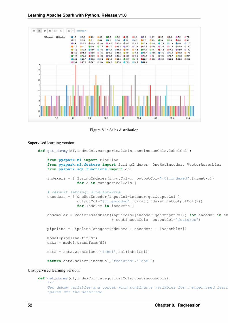
Figure 8.1: Sales distribution
Supervised learning version:
def get_dummy(df,indexCol,categoricalCols,continuousCols,labelCol):
from pyspark.ml import Pipelinefrom pyspark.ml.feature import StringIndexer, OneHotEncoder, VectorAssemblerfrom pyspark.sql.functions import col
indexers = [ StringIndexer(inputCol=c, outputCol="{0}_indexed".format(c))for c in categoricalCols ]
# default setting: dropLast=Trueencoders = [ OneHotEncoder(inputCol=indexer.getOutputCol(),
outputCol="{0}_encoded".format(indexer.getOutputCol()))for indexer in indexers ]
assembler = VectorAssembler(inputCols=[encoder.getOutputCol() for encoder in encoders]+ continuousCols, outputCol="features")
pipeline = Pipeline(stages=indexers + encoders + [assembler])
model=pipeline.fit(df)data = model.transform(df)
data = data.withColumn(’label’,col(labelCol))
return data.select(indexCol,’features’,’label’)
Unsupervised learning version:
def get_dummy(df,indexCol,categoricalCols,continuousCols):’’’Get dummy variables and concat with continuous variables for unsupervised learning.:param df: the dataframe
52 Chapter 8. Regression
Learning Apache Spark with Python, Release v1.0
:param categoricalCols: the name list of the categorical data:param continuousCols: the name list of the numerical data:return k: feature matrix
:author: Wenqiang Feng:email: [email protected]’’’
indexers = [ StringIndexer(inputCol=c, outputCol="{0}_indexed".format(c))for c in categoricalCols ]
# default setting: dropLast=Trueencoders = [ OneHotEncoder(inputCol=indexer.getOutputCol(),
outputCol="{0}_encoded".format(indexer.getOutputCol()))for indexer in indexers ]
assembler = VectorAssembler(inputCols=[encoder.getOutputCol() for encoder in encoders]+ continuousCols, outputCol="features")
pipeline = Pipeline(stages=indexers + encoders + [assembler])
model=pipeline.fit(df)data = model.transform(df)
return data.select(indexCol,’features’)
4. Transform the dataset to DataFrame
transformed= transData(df)transformed.show(5)
+-----------------+-----+| features|label|+-----------------+-----+|[230.1,37.8,69.2]| 22.1|| [44.5,39.3,45.1]| 10.4|| [17.2,45.9,69.3]| 9.3||[151.5,41.3,58.5]| 18.5||[180.8,10.8,58.4]| 12.9|+-----------------+-----+only showing top 5 rows
Note: You will find out that all of the supervised machine learning algorithms in Spark are based onthe features and label (unsupervised machine learning algorithms in Spark are based on the features).That is to say, you can play with all of the machine learning algorithms in Spark when you get ready thefeatures and label in pipeline architecture.
5. Deal With Categorical Variables
from pyspark.ml import Pipelinefrom pyspark.ml.regression import LinearRegressionfrom pyspark.ml.feature import VectorIndexerfrom pyspark.ml.evaluation import RegressionEvaluator
# Automatically identify categorical features, and index them.# We specify maxCategories so features with > 4 distinct values are treated as continuous.
8.1. Linear Regression 53
Learning Apache Spark with Python, Release v1.0
featureIndexer = VectorIndexer(inputCol="features", \outputCol="indexedFeatures",\maxCategories=4).fit(transformed)
data = featureIndexer.transform(transformed)
Now you check your dataset with
data.show(5,True)
you will get
+-----------------+-----+-----------------+| features|label| indexedFeatures|+-----------------+-----+-----------------+|[230.1,37.8,69.2]| 22.1|[230.1,37.8,69.2]|| [44.5,39.3,45.1]| 10.4| [44.5,39.3,45.1]|| [17.2,45.9,69.3]| 9.3| [17.2,45.9,69.3]||[151.5,41.3,58.5]| 18.5|[151.5,41.3,58.5]||[180.8,10.8,58.4]| 12.9|[180.8,10.8,58.4]|+-----------------+-----+-----------------+only showing top 5 rows
6. Split the data into training and test sets (40% held out for testing)
# Split the data into training and test sets (40% held out for testing)(trainingData, testData) = transformed.randomSplit([0.6, 0.4])
You can check your train and test data as follows (In my opinion, it is always to good to keep trackingyour data during prototype pahse):
trainingData.show(5)testData.show(5)
Then you will get
+---------------+-----+---------------+| features|label|indexedFeatures|+---------------+-----+---------------+| [4.1,11.6,5.7]| 3.2| [4.1,11.6,5.7]|| [5.4,29.9,9.4]| 5.3| [5.4,29.9,9.4]||[7.3,28.1,41.4]| 5.5|[7.3,28.1,41.4]||[7.8,38.9,50.6]| 6.6|[7.8,38.9,50.6]|| [8.6,2.1,1.0]| 4.8| [8.6,2.1,1.0]|+---------------+-----+---------------+only showing top 5 rows
+----------------+-----+----------------+| features|label| indexedFeatures|+----------------+-----+----------------+| [0.7,39.6,8.7]| 1.6| [0.7,39.6,8.7]|| [8.4,27.2,2.1]| 5.7| [8.4,27.2,2.1]||[11.7,36.9,45.2]| 7.3|[11.7,36.9,45.2]||[13.2,15.9,49.6]| 5.6|[13.2,15.9,49.6]||[16.9,43.7,89.4]| 8.7|[16.9,43.7,89.4]|+----------------+-----+----------------+only showing top 5 rows
7. Fit Ordinary Least Square Regression Model
54 Chapter 8. Regression
Learning Apache Spark with Python, Release v1.0
For more details about the parameters, please visit Linear Regression API .
# Import LinearRegression classfrom pyspark.ml.regression import LinearRegression
# Define LinearRegression algorithmlr = LinearRegression()
8. Pipeline Architecture
# Chain indexer and tree in a Pipelinepipeline = Pipeline(stages=[featureIndexer, lr])
model = pipeline.fit(trainingData)
9. Summary of the Model
Spark has a poor summary function for data and model. I wrote a summary function which has similarformat as R output for the linear regression in PySpark.
def modelsummary(model):import numpy as npprint ("Note: the last rows are the information for Intercept")print ("##","-------------------------------------------------")print ("##"," Estimate | Std.Error | t Values | P-value")coef = np.append(list(model.coefficients),model.intercept)Summary=model.summary
for i in range(len(Summary.pValues)):print ("##",’{:10.6f}’.format(coef[i]),\’{:10.6f}’.format(Summary.coefficientStandardErrors[i]),\’{:8.3f}’.format(Summary.tValues[i]),\’{:10.6f}’.format(Summary.pValues[i]))
print ("##",’---’)print ("##","Mean squared error: % .6f" \
% Summary.meanSquaredError, ", RMSE: % .6f" \% Summary.rootMeanSquaredError )
print ("##","Multiple R-squared: %f" % Summary.r2, ", \Total iterations: %i"% Summary.totalIterations)
modelsummary(model.stages[-1])
You will get the following summary results:
Note: the last rows are the information for Intercept(’##’, ’-------------------------------------------------’)(’##’, ’ Estimate | Std.Error | t Values | P-value’)(’##’, ’ 0.044186’, ’ 0.001663’, ’ 26.573’, ’ 0.000000’)(’##’, ’ 0.206311’, ’ 0.010846’, ’ 19.022’, ’ 0.000000’)(’##’, ’ 0.001963’, ’ 0.007467’, ’ 0.263’, ’ 0.793113’)(’##’, ’ 2.596154’, ’ 0.379550’, ’ 6.840’, ’ 0.000000’)(’##’, ’---’)(’##’, ’Mean squared error: 2.588230’, ’, RMSE: 1.608798’)(’##’, ’Multiple R-squared: 0.911869’, ’, Total iterations: 1’)
10. Make predictions
8.1. Linear Regression 55
Learning Apache Spark with Python, Release v1.0
# Make predictions.predictions = model.transform(testData)
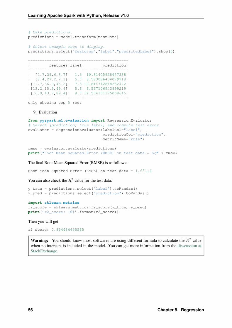
# Select example rows to display.predictions.select("features","label","predictedLabel").show(5)
+----------------+-----+------------------+| features|label| prediction|+----------------+-----+------------------+| [0.7,39.6,8.7]| 1.6| 10.81405928637388|| [8.4,27.2,2.1]| 5.7| 8.583086404079918||[11.7,36.9,45.2]| 7.3|10.814712818232422||[13.2,15.9,49.6]| 5.6| 6.557106943899219||[16.9,43.7,89.4]| 8.7|12.534151375058645|+----------------+-----+------------------+only showing top 5 rows
9. Evaluation
from pyspark.ml.evaluation import RegressionEvaluator# Select (prediction, true label) and compute test errorevaluator = RegressionEvaluator(labelCol="label",
predictionCol="prediction",metricName="rmse")
rmse = evaluator.evaluate(predictions)print("Root Mean Squared Error (RMSE) on test data = %g" % rmse)
The final Root Mean Squared Error (RMSE) is as follows:
Root Mean Squared Error (RMSE) on test data = 1.63114
You can also check the 𝑅2 value for the test data:
y_true = predictions.select("label").toPandas()y_pred = predictions.select("prediction").toPandas()
import sklearn.metricsr2_score = sklearn.metrics.r2_score(y_true, y_pred)print(’r2_score: {0}’.format(r2_score))
Then you will get
r2_score: 0.854486655585
Warning: You should know most softwares are using different formula to calculate the 𝑅2 valuewhen no intercept is included in the model. You can get more information from the disscussion atStackExchange.
56 Chapter 8. Regression
Learning Apache Spark with Python, Release v1.0
8.2 Generalized linear regression
8.2.1 Introduction
8.2.2 How to solve it?
8.2.3 Demo
• The Jupyter notebook can be download from Generalized Linear Regression.
• For more details about the parameters, please visit Generalized Linear Regression API .
1. Set up spark context and SparkSession
from pyspark.sql import SparkSession
spark = SparkSession \.builder \.appName("Python Spark regression example") \.config("spark.some.config.option", "some-value") \.getOrCreate()
2. Load dataset
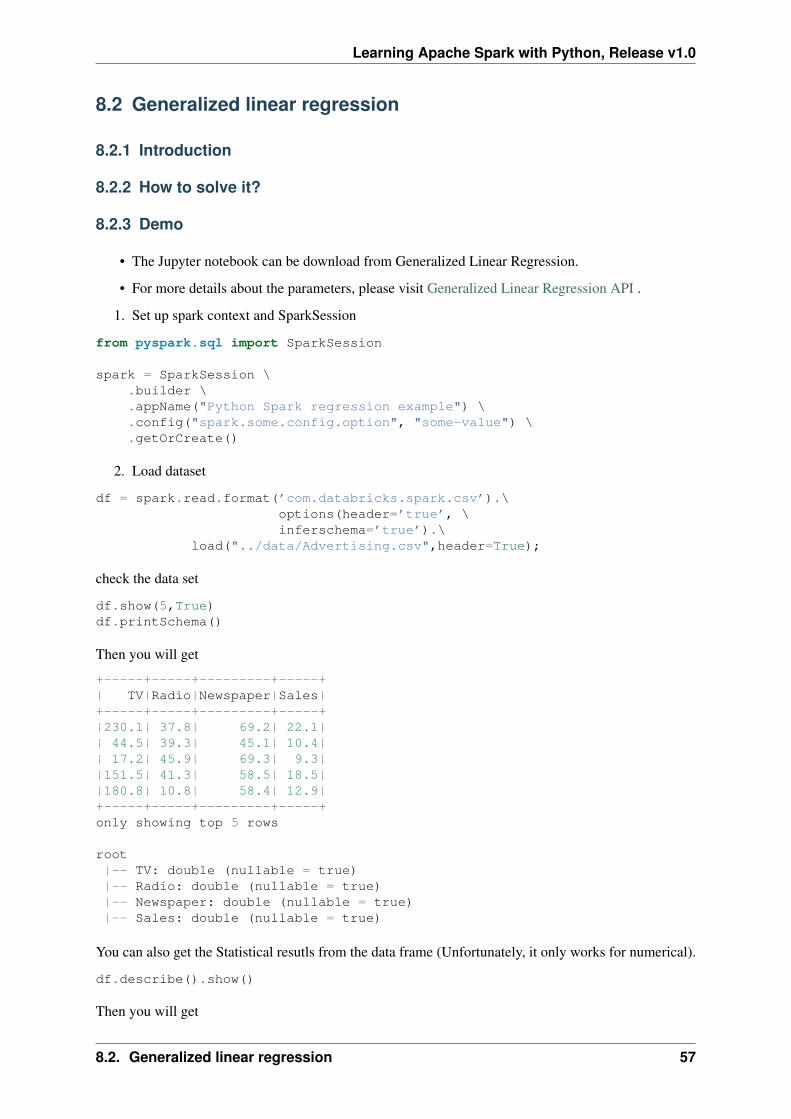
df = spark.read.format(’com.databricks.spark.csv’).\options(header=’true’, \inferschema=’true’).\
load("../data/Advertising.csv",header=True);
check the data set
df.show(5,True)df.printSchema()
Then you will get
+-----+-----+---------+-----+| TV|Radio|Newspaper|Sales|+-----+-----+---------+-----+|230.1| 37.8| 69.2| 22.1|| 44.5| 39.3| 45.1| 10.4|| 17.2| 45.9| 69.3| 9.3||151.5| 41.3| 58.5| 18.5||180.8| 10.8| 58.4| 12.9|+-----+-----+---------+-----+only showing top 5 rows
root|-- TV: double (nullable = true)|-- Radio: double (nullable = true)|-- Newspaper: double (nullable = true)|-- Sales: double (nullable = true)
You can also get the Statistical resutls from the data frame (Unfortunately, it only works for numerical).
df.describe().show()
Then you will get
8.2. Generalized linear regression 57
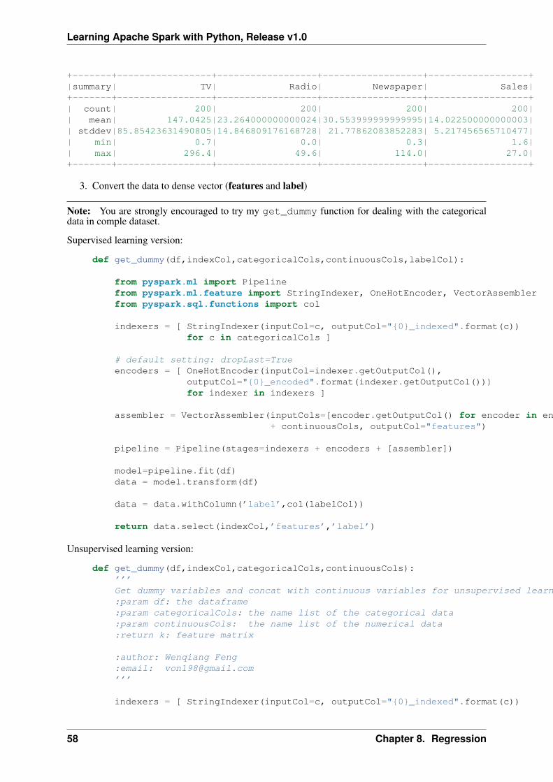
Learning Apache Spark with Python, Release v1.0
+-------+-----------------+------------------+------------------+------------------+|summary| TV| Radio| Newspaper| Sales|+-------+-----------------+------------------+------------------+------------------+| count| 200| 200| 200| 200|| mean| 147.0425|23.264000000000024|30.553999999999995|14.022500000000003|| stddev|85.85423631490805|14.846809176168728| 21.77862083852283| 5.217456565710477|| min| 0.7| 0.0| 0.3| 1.6|| max| 296.4| 49.6| 114.0| 27.0|+-------+-----------------+------------------+------------------+------------------+
3. Convert the data to dense vector (features and label)
Note: You are strongly encouraged to try my get_dummy function for dealing with the categoricaldata in comple dataset.
Supervised learning version:
def get_dummy(df,indexCol,categoricalCols,continuousCols,labelCol):
from pyspark.ml import Pipelinefrom pyspark.ml.feature import StringIndexer, OneHotEncoder, VectorAssemblerfrom pyspark.sql.functions import col
indexers = [ StringIndexer(inputCol=c, outputCol="{0}_indexed".format(c))for c in categoricalCols ]
# default setting: dropLast=Trueencoders = [ OneHotEncoder(inputCol=indexer.getOutputCol(),
outputCol="{0}_encoded".format(indexer.getOutputCol()))for indexer in indexers ]
assembler = VectorAssembler(inputCols=[encoder.getOutputCol() for encoder in encoders]+ continuousCols, outputCol="features")
pipeline = Pipeline(stages=indexers + encoders + [assembler])
model=pipeline.fit(df)data = model.transform(df)
data = data.withColumn(’label’,col(labelCol))
return data.select(indexCol,’features’,’label’)
Unsupervised learning version:
def get_dummy(df,indexCol,categoricalCols,continuousCols):’’’Get dummy variables and concat with continuous variables for unsupervised learning.:param df: the dataframe:param categoricalCols: the name list of the categorical data:param continuousCols: the name list of the numerical data:return k: feature matrix
:author: Wenqiang Feng:email: [email protected]’’’
indexers = [ StringIndexer(inputCol=c, outputCol="{0}_indexed".format(c))
58 Chapter 8. Regression
Learning Apache Spark with Python, Release v1.0
for c in categoricalCols ]
# default setting: dropLast=Trueencoders = [ OneHotEncoder(inputCol=indexer.getOutputCol(),
outputCol="{0}_encoded".format(indexer.getOutputCol()))for indexer in indexers ]
assembler = VectorAssembler(inputCols=[encoder.getOutputCol() for encoder in encoders]+ continuousCols, outputCol="features")
pipeline = Pipeline(stages=indexers + encoders + [assembler])
model=pipeline.fit(df)data = model.transform(df)
return data.select(indexCol,’features’)
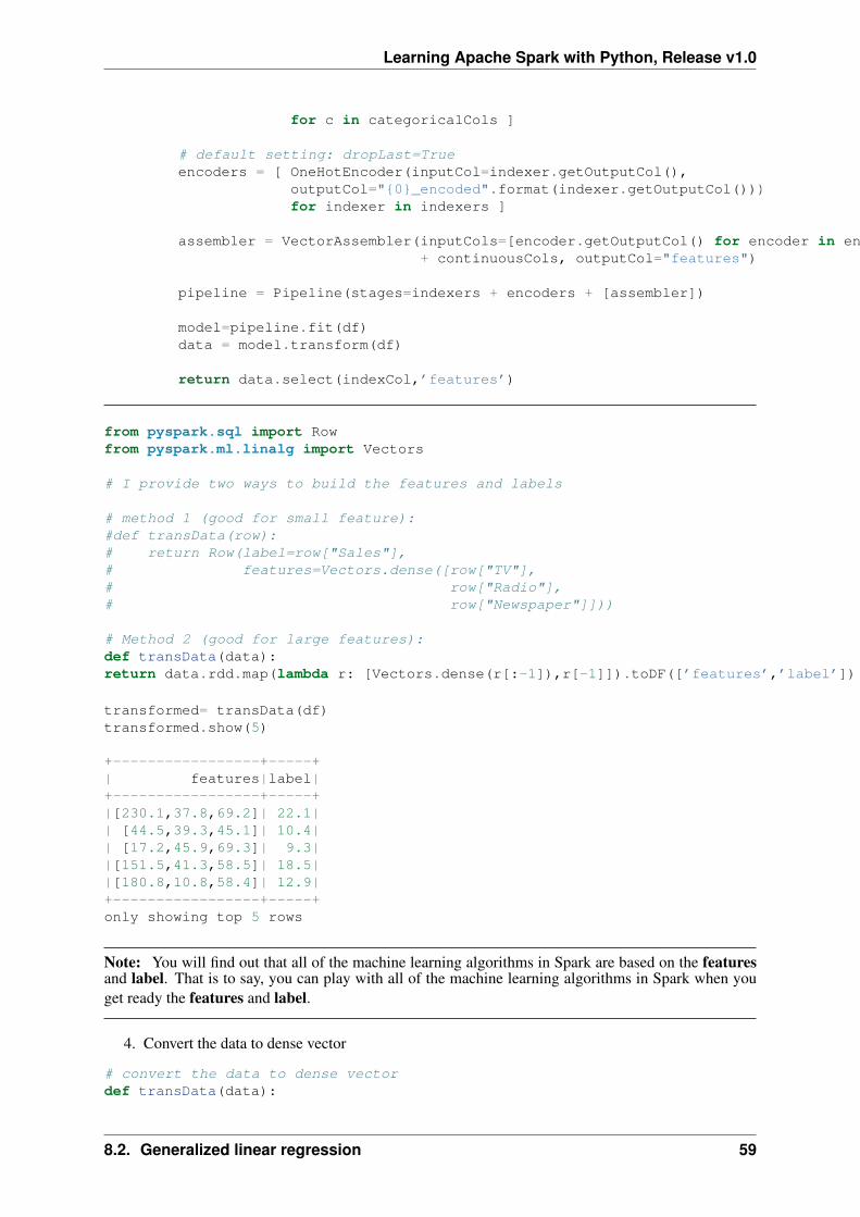
from pyspark.sql import Rowfrom pyspark.ml.linalg import Vectors
# I provide two ways to build the features and labels
# method 1 (good for small feature):#def transData(row):# return Row(label=row["Sales"],# features=Vectors.dense([row["TV"],# row["Radio"],# row["Newspaper"]]))
# Method 2 (good for large features):def transData(data):return data.rdd.map(lambda r: [Vectors.dense(r[:-1]),r[-1]]).toDF([’features’,’label’])
transformed= transData(df)transformed.show(5)
+-----------------+-----+| features|label|+-----------------+-----+|[230.1,37.8,69.2]| 22.1|| [44.5,39.3,45.1]| 10.4|| [17.2,45.9,69.3]| 9.3||[151.5,41.3,58.5]| 18.5||[180.8,10.8,58.4]| 12.9|+-----------------+-----+only showing top 5 rows
Note: You will find out that all of the machine learning algorithms in Spark are based on the featuresand label. That is to say, you can play with all of the machine learning algorithms in Spark when youget ready the features and label.
4. Convert the data to dense vector
# convert the data to dense vectordef transData(data):
8.2. Generalized linear regression 59
Learning Apache Spark with Python, Release v1.0
return data.rdd.map(lambda r: [r[-1], Vectors.dense(r[:-1])]).\toDF([’label’,’features’])
from pyspark.sql import Rowfrom pyspark.ml.linalg import Vectors
data= transData(df)data.show()
5. Deal with the Categorical variables
from pyspark.ml import Pipelinefrom pyspark.ml.regression import LinearRegressionfrom pyspark.ml.feature import VectorIndexerfrom pyspark.ml.evaluation import RegressionEvaluator
# Automatically identify categorical features, and index them.# We specify maxCategories so features with > 4# distinct values are treated as continuous.
featureIndexer = VectorIndexer(inputCol="features", \outputCol="indexedFeatures",\maxCategories=4).fit(transformed)
data = featureIndexer.transform(transformed)
When you check you data at this point, you will get
+-----------------+-----+-----------------+| features|label| indexedFeatures|+-----------------+-----+-----------------+|[230.1,37.8,69.2]| 22.1|[230.1,37.8,69.2]|| [44.5,39.3,45.1]| 10.4| [44.5,39.3,45.1]|| [17.2,45.9,69.3]| 9.3| [17.2,45.9,69.3]||[151.5,41.3,58.5]| 18.5|[151.5,41.3,58.5]||[180.8,10.8,58.4]| 12.9|[180.8,10.8,58.4]|+-----------------+-----+-----------------+only showing top 5 rows
6. Split the data into training and test sets (40% held out for testing)
# Split the data into training and test sets (40% held out for testing)(trainingData, testData) = transformed.randomSplit([0.6, 0.4])
You can check your train and test data as follows (In my opinion, it is always to good to keep trackingyour data during prototype pahse):
trainingData.show(5)testData.show(5)
Then you will get
+----------------+-----+----------------+| features|label| indexedFeatures|+----------------+-----+----------------+| [5.4,29.9,9.4]| 5.3| [5.4,29.9,9.4]|| [7.8,38.9,50.6]| 6.6| [7.8,38.9,50.6]|| [8.4,27.2,2.1]| 5.7| [8.4,27.2,2.1]|| [8.7,48.9,75.0]| 7.2| [8.7,48.9,75.0]|
60 Chapter 8. Regression
Learning Apache Spark with Python, Release v1.0
|[11.7,36.9,45.2]| 7.3|[11.7,36.9,45.2]|+----------------+-----+----------------+only showing top 5 rows
+---------------+-----+---------------+| features|label|indexedFeatures|+---------------+-----+---------------+| [0.7,39.6,8.7]| 1.6| [0.7,39.6,8.7]|| [4.1,11.6,5.7]| 3.2| [4.1,11.6,5.7]||[7.3,28.1,41.4]| 5.5|[7.3,28.1,41.4]|| [8.6,2.1,1.0]| 4.8| [8.6,2.1,1.0]||[17.2,4.1,31.6]| 5.9|[17.2,4.1,31.6]|+---------------+-----+---------------+only showing top 5 rows
7. Fit Generalized Linear Regression Model
# Import LinearRegression classfrom pyspark.ml.regression import GeneralizedLinearRegression
# Define LinearRegression algorithmglr = GeneralizedLinearRegression(family="gaussian", link="identity",\
maxIter=10, regParam=0.3)
8. Pipeline Architecture
# Chain indexer and tree in a Pipelinepipeline = Pipeline(stages=[featureIndexer, glr])
model = pipeline.fit(trainingData)
9. Summary of the Model
Spark has a poor summary function for data and model. I wrote a summary function which has similarformat as R output for the linear regression in PySpark.
def modelsummary(model):import numpy as npprint ("Note: the last rows are the information for Intercept")print ("##","-------------------------------------------------")print ("##"," Estimate | Std.Error | t Values | P-value")coef = np.append(list(model.coefficients),model.intercept)Summary=model.summary
for i in range(len(Summary.pValues)):print ("##",’{:10.6f}’.format(coef[i]),\’{:10.6f}’.format(Summary.coefficientStandardErrors[i]),\’{:8.3f}’.format(Summary.tValues[i]),\’{:10.6f}’.format(Summary.pValues[i]))
print ("##",’---’)# print ("##","Mean squared error: % .6f" \# % Summary.meanSquaredError, ", RMSE: % .6f" \# % Summary.rootMeanSquaredError )# print ("##","Multiple R-squared: %f" % Summary.r2, ", \# Total iterations: %i"% Summary.totalIterations)
8.2. Generalized linear regression 61
Learning Apache Spark with Python, Release v1.0
modelsummary(model.stages[-1])
You will get the following summary results:
Note: the last rows are the information for Intercept(’##’, ’-------------------------------------------------’)(’##’, ’ Estimate | Std.Error | t Values | P-value’)(’##’, ’ 0.042857’, ’ 0.001668’, ’ 25.692’, ’ 0.000000’)(’##’, ’ 0.199922’, ’ 0.009881’, ’ 20.232’, ’ 0.000000’)(’##’, ’ -0.001957’, ’ 0.006917’, ’ -0.283’, ’ 0.777757’)(’##’, ’ 3.007515’, ’ 0.406389’, ’ 7.401’, ’ 0.000000’)(’##’, ’---’)
10. Make predictions
# Make predictions.predictions = model.transform(testData)
# Select example rows to display.predictions.select("features","label","predictedLabel").show(5)
+---------------+-----+------------------+| features|label| prediction|+---------------+-----+------------------+| [0.7,39.6,8.7]| 1.6|10.937383732327625|| [4.1,11.6,5.7]| 3.2| 5.491166258750164||[7.3,28.1,41.4]| 5.5| 8.8571603947873|| [8.6,2.1,1.0]| 4.8| 3.793966281660073||[17.2,4.1,31.6]| 5.9| 4.502507124763654|+---------------+-----+------------------+only showing top 5 rows
11. Evaluation
from pyspark.ml.evaluation import RegressionEvaluatorfrom pyspark.ml.evaluation import RegressionEvaluator# Select (prediction, true label) and compute test errorevaluator = RegressionEvaluator(labelCol="label",
predictionCol="prediction",metricName="rmse")
rmse = evaluator.evaluate(predictions)print("Root Mean Squared Error (RMSE) on test data = %g" % rmse)
The final Root Mean Squared Error (RMSE) is as follows:
Root Mean Squared Error (RMSE) on test data = 1.89857
y_true = predictions.select("label").toPandas()y_pred = predictions.select("prediction").toPandas()
import sklearn.metricsr2_score = sklearn.metrics.r2_score(y_true, y_pred)print(’r2_score: {0}’.format(r2_score))
Then you will get the 𝑅2 value:
62 Chapter 8. Regression
Learning Apache Spark with Python, Release v1.0
r2_score: 0.87707391843
8.3 Decision tree Regression
8.3.1 Introduction
8.3.2 How to solve it?
8.3.3 Demo
• The Jupyter notebook can be download from Decision Tree Regression.
• For more details about the parameters, please visit Decision Tree Regressor API .
1. Set up spark context and SparkSession
from pyspark.sql import SparkSession
spark = SparkSession \.builder \.appName("Python Spark regression example") \.config("spark.some.config.option", "some-value") \.getOrCreate()
2. Load dataset
df = spark.read.format(’com.databricks.spark.csv’).\options(header=’true’, \inferschema=’true’).\
load("../data/Advertising.csv",header=True);
check the data set
df.show(5,True)df.printSchema()
Then you will get
+-----+-----+---------+-----+| TV|Radio|Newspaper|Sales|+-----+-----+---------+-----+|230.1| 37.8| 69.2| 22.1|| 44.5| 39.3| 45.1| 10.4|| 17.2| 45.9| 69.3| 9.3||151.5| 41.3| 58.5| 18.5||180.8| 10.8| 58.4| 12.9|+-----+-----+---------+-----+only showing top 5 rows
root|-- TV: double (nullable = true)|-- Radio: double (nullable = true)|-- Newspaper: double (nullable = true)|-- Sales: double (nullable = true)
8.3. Decision tree Regression 63
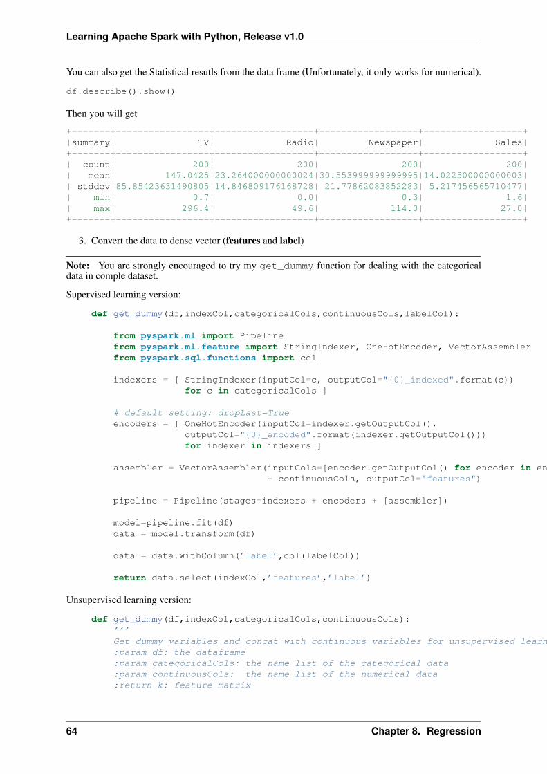
Learning Apache Spark with Python, Release v1.0
You can also get the Statistical resutls from the data frame (Unfortunately, it only works for numerical).
df.describe().show()
Then you will get
+-------+-----------------+------------------+------------------+------------------+|summary| TV| Radio| Newspaper| Sales|+-------+-----------------+------------------+------------------+------------------+| count| 200| 200| 200| 200|| mean| 147.0425|23.264000000000024|30.553999999999995|14.022500000000003|| stddev|85.85423631490805|14.846809176168728| 21.77862083852283| 5.217456565710477|| min| 0.7| 0.0| 0.3| 1.6|| max| 296.4| 49.6| 114.0| 27.0|+-------+-----------------+------------------+------------------+------------------+
3. Convert the data to dense vector (features and label)
Note: You are strongly encouraged to try my get_dummy function for dealing with the categoricaldata in comple dataset.
Supervised learning version:
def get_dummy(df,indexCol,categoricalCols,continuousCols,labelCol):
from pyspark.ml import Pipelinefrom pyspark.ml.feature import StringIndexer, OneHotEncoder, VectorAssemblerfrom pyspark.sql.functions import col
indexers = [ StringIndexer(inputCol=c, outputCol="{0}_indexed".format(c))for c in categoricalCols ]
# default setting: dropLast=Trueencoders = [ OneHotEncoder(inputCol=indexer.getOutputCol(),
outputCol="{0}_encoded".format(indexer.getOutputCol()))for indexer in indexers ]
assembler = VectorAssembler(inputCols=[encoder.getOutputCol() for encoder in encoders]+ continuousCols, outputCol="features")
pipeline = Pipeline(stages=indexers + encoders + [assembler])
model=pipeline.fit(df)data = model.transform(df)
data = data.withColumn(’label’,col(labelCol))
return data.select(indexCol,’features’,’label’)
Unsupervised learning version:
def get_dummy(df,indexCol,categoricalCols,continuousCols):’’’Get dummy variables and concat with continuous variables for unsupervised learning.:param df: the dataframe:param categoricalCols: the name list of the categorical data:param continuousCols: the name list of the numerical data:return k: feature matrix
64 Chapter 8. Regression
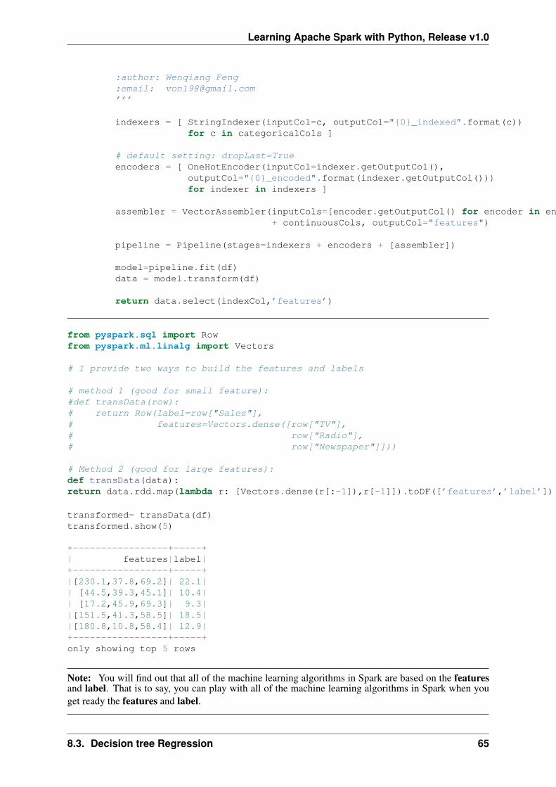
Learning Apache Spark with Python, Release v1.0
:author: Wenqiang Feng:email: [email protected]’’’
indexers = [ StringIndexer(inputCol=c, outputCol="{0}_indexed".format(c))for c in categoricalCols ]
# default setting: dropLast=Trueencoders = [ OneHotEncoder(inputCol=indexer.getOutputCol(),
outputCol="{0}_encoded".format(indexer.getOutputCol()))for indexer in indexers ]
assembler = VectorAssembler(inputCols=[encoder.getOutputCol() for encoder in encoders]+ continuousCols, outputCol="features")
pipeline = Pipeline(stages=indexers + encoders + [assembler])
model=pipeline.fit(df)data = model.transform(df)
return data.select(indexCol,’features’)
from pyspark.sql import Rowfrom pyspark.ml.linalg import Vectors
# I provide two ways to build the features and labels
# method 1 (good for small feature):#def transData(row):# return Row(label=row["Sales"],# features=Vectors.dense([row["TV"],# row["Radio"],# row["Newspaper"]]))
# Method 2 (good for large features):def transData(data):return data.rdd.map(lambda r: [Vectors.dense(r[:-1]),r[-1]]).toDF([’features’,’label’])
transformed= transData(df)transformed.show(5)
+-----------------+-----+| features|label|+-----------------+-----+|[230.1,37.8,69.2]| 22.1|| [44.5,39.3,45.1]| 10.4|| [17.2,45.9,69.3]| 9.3||[151.5,41.3,58.5]| 18.5||[180.8,10.8,58.4]| 12.9|+-----------------+-----+only showing top 5 rows
Note: You will find out that all of the machine learning algorithms in Spark are based on the featuresand label. That is to say, you can play with all of the machine learning algorithms in Spark when youget ready the features and label.
8.3. Decision tree Regression 65
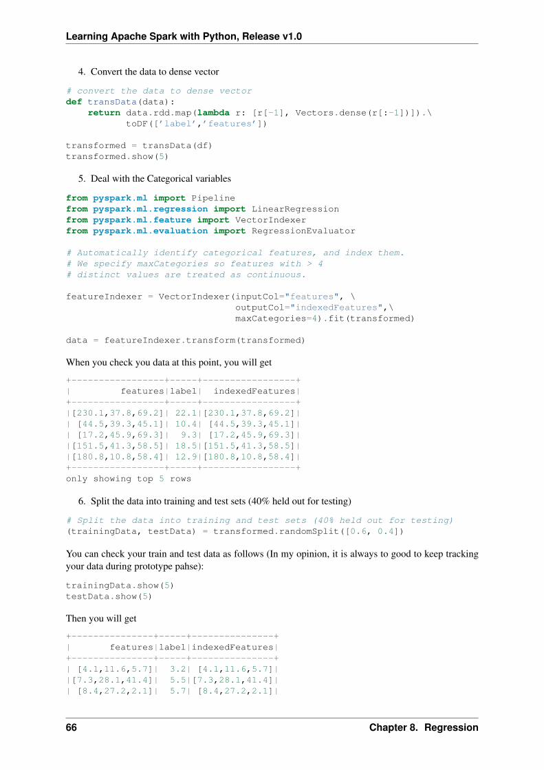
Learning Apache Spark with Python, Release v1.0
4. Convert the data to dense vector
# convert the data to dense vectordef transData(data):
return data.rdd.map(lambda r: [r[-1], Vectors.dense(r[:-1])]).\toDF([’label’,’features’])
transformed = transData(df)transformed.show(5)
5. Deal with the Categorical variables
from pyspark.ml import Pipelinefrom pyspark.ml.regression import LinearRegressionfrom pyspark.ml.feature import VectorIndexerfrom pyspark.ml.evaluation import RegressionEvaluator
# Automatically identify categorical features, and index them.# We specify maxCategories so features with > 4# distinct values are treated as continuous.
featureIndexer = VectorIndexer(inputCol="features", \outputCol="indexedFeatures",\maxCategories=4).fit(transformed)
data = featureIndexer.transform(transformed)
When you check you data at this point, you will get
+-----------------+-----+-----------------+| features|label| indexedFeatures|+-----------------+-----+-----------------+|[230.1,37.8,69.2]| 22.1|[230.1,37.8,69.2]|| [44.5,39.3,45.1]| 10.4| [44.5,39.3,45.1]|| [17.2,45.9,69.3]| 9.3| [17.2,45.9,69.3]||[151.5,41.3,58.5]| 18.5|[151.5,41.3,58.5]||[180.8,10.8,58.4]| 12.9|[180.8,10.8,58.4]|+-----------------+-----+-----------------+only showing top 5 rows
6. Split the data into training and test sets (40% held out for testing)
# Split the data into training and test sets (40% held out for testing)(trainingData, testData) = transformed.randomSplit([0.6, 0.4])
You can check your train and test data as follows (In my opinion, it is always to good to keep trackingyour data during prototype pahse):
trainingData.show(5)testData.show(5)
Then you will get
+---------------+-----+---------------+| features|label|indexedFeatures|+---------------+-----+---------------+| [4.1,11.6,5.7]| 3.2| [4.1,11.6,5.7]||[7.3,28.1,41.4]| 5.5|[7.3,28.1,41.4]|| [8.4,27.2,2.1]| 5.7| [8.4,27.2,2.1]|
66 Chapter 8. Regression
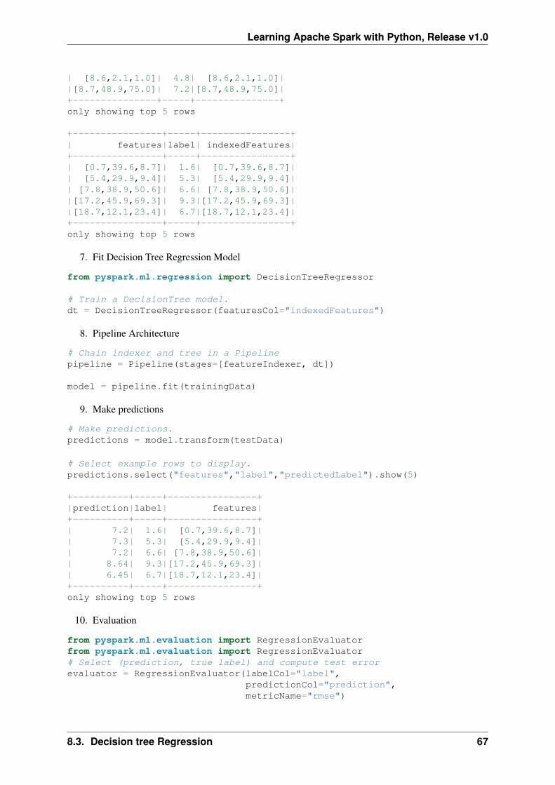
Learning Apache Spark with Python, Release v1.0
| [8.6,2.1,1.0]| 4.8| [8.6,2.1,1.0]||[8.7,48.9,75.0]| 7.2|[8.7,48.9,75.0]|+---------------+-----+---------------+only showing top 5 rows
+----------------+-----+----------------+| features|label| indexedFeatures|+----------------+-----+----------------+| [0.7,39.6,8.7]| 1.6| [0.7,39.6,8.7]|| [5.4,29.9,9.4]| 5.3| [5.4,29.9,9.4]|| [7.8,38.9,50.6]| 6.6| [7.8,38.9,50.6]||[17.2,45.9,69.3]| 9.3|[17.2,45.9,69.3]||[18.7,12.1,23.4]| 6.7|[18.7,12.1,23.4]|+----------------+-----+----------------+only showing top 5 rows
7. Fit Decision Tree Regression Model
from pyspark.ml.regression import DecisionTreeRegressor
# Train a DecisionTree model.dt = DecisionTreeRegressor(featuresCol="indexedFeatures")
8. Pipeline Architecture
# Chain indexer and tree in a Pipelinepipeline = Pipeline(stages=[featureIndexer, dt])
model = pipeline.fit(trainingData)
9. Make predictions
# Make predictions.predictions = model.transform(testData)
# Select example rows to display.predictions.select("features","label","predictedLabel").show(5)
+----------+-----+----------------+|prediction|label| features|+----------+-----+----------------+| 7.2| 1.6| [0.7,39.6,8.7]|| 7.3| 5.3| [5.4,29.9,9.4]|| 7.2| 6.6| [7.8,38.9,50.6]|| 8.64| 9.3|[17.2,45.9,69.3]|| 6.45| 6.7|[18.7,12.1,23.4]|+----------+-----+----------------+only showing top 5 rows
10. Evaluation
from pyspark.ml.evaluation import RegressionEvaluatorfrom pyspark.ml.evaluation import RegressionEvaluator# Select (prediction, true label) and compute test errorevaluator = RegressionEvaluator(labelCol="label",
predictionCol="prediction",metricName="rmse")
8.3. Decision tree Regression 67
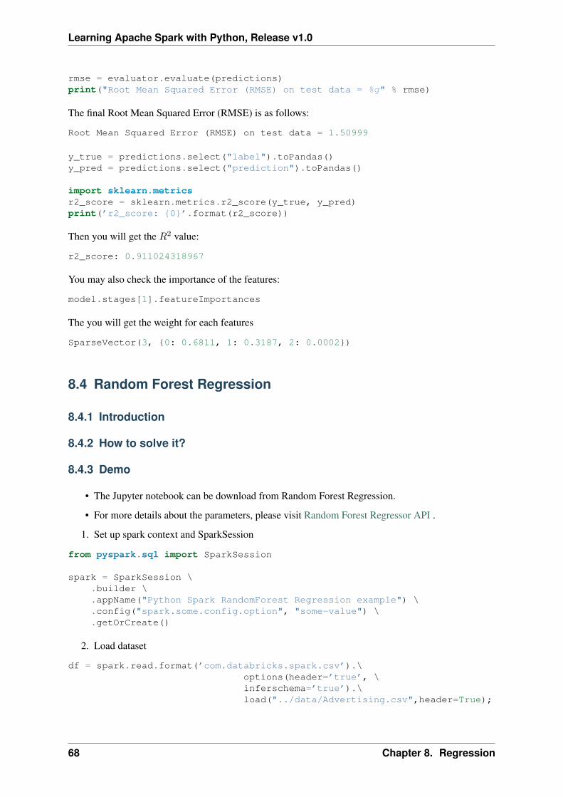
Learning Apache Spark with Python, Release v1.0
rmse = evaluator.evaluate(predictions)print("Root Mean Squared Error (RMSE) on test data = %g" % rmse)
The final Root Mean Squared Error (RMSE) is as follows:
Root Mean Squared Error (RMSE) on test data = 1.50999
y_true = predictions.select("label").toPandas()y_pred = predictions.select("prediction").toPandas()
import sklearn.metricsr2_score = sklearn.metrics.r2_score(y_true, y_pred)print(’r2_score: {0}’.format(r2_score))
Then you will get the 𝑅2 value:
r2_score: 0.911024318967
You may also check the importance of the features:
model.stages[1].featureImportances
The you will get the weight for each features
SparseVector(3, {0: 0.6811, 1: 0.3187, 2: 0.0002})
8.4 Random Forest Regression
8.4.1 Introduction
8.4.2 How to solve it?
8.4.3 Demo
• The Jupyter notebook can be download from Random Forest Regression.
• For more details about the parameters, please visit Random Forest Regressor API .
1. Set up spark context and SparkSession
from pyspark.sql import SparkSession
spark = SparkSession \.builder \.appName("Python Spark RandomForest Regression example") \.config("spark.some.config.option", "some-value") \.getOrCreate()
2. Load dataset
df = spark.read.format(’com.databricks.spark.csv’).\options(header=’true’, \inferschema=’true’).\load("../data/Advertising.csv",header=True);
68 Chapter 8. Regression
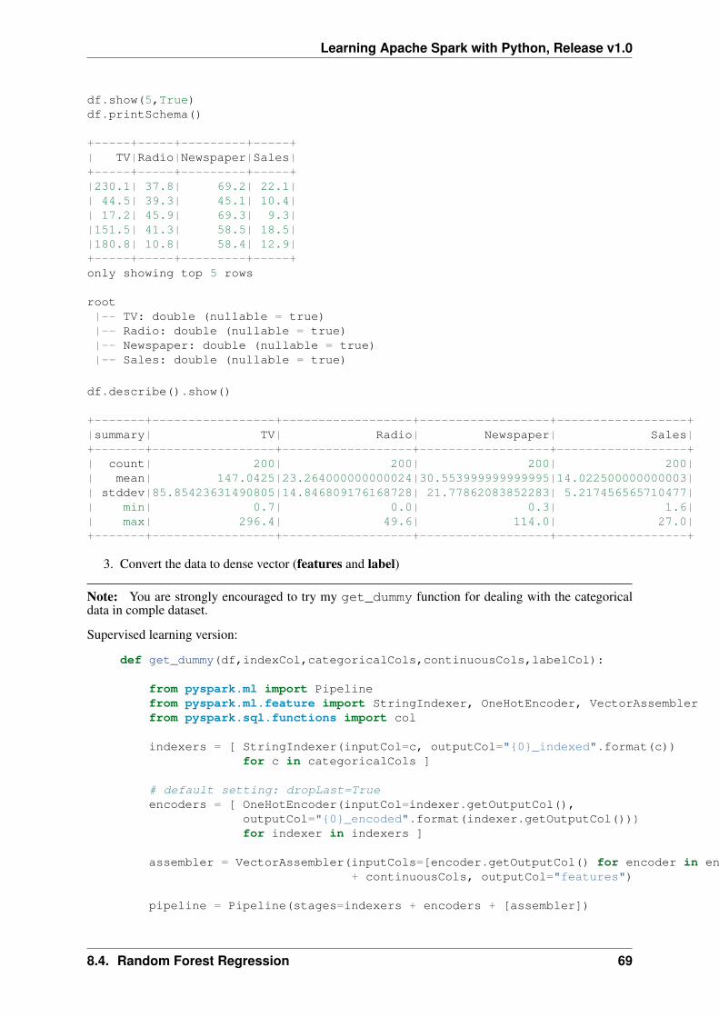
Learning Apache Spark with Python, Release v1.0
df.show(5,True)df.printSchema()
+-----+-----+---------+-----+| TV|Radio|Newspaper|Sales|+-----+-----+---------+-----+|230.1| 37.8| 69.2| 22.1|| 44.5| 39.3| 45.1| 10.4|| 17.2| 45.9| 69.3| 9.3||151.5| 41.3| 58.5| 18.5||180.8| 10.8| 58.4| 12.9|+-----+-----+---------+-----+only showing top 5 rows
root|-- TV: double (nullable = true)|-- Radio: double (nullable = true)|-- Newspaper: double (nullable = true)|-- Sales: double (nullable = true)
df.describe().show()
+-------+-----------------+------------------+------------------+------------------+|summary| TV| Radio| Newspaper| Sales|+-------+-----------------+------------------+------------------+------------------+| count| 200| 200| 200| 200|| mean| 147.0425|23.264000000000024|30.553999999999995|14.022500000000003|| stddev|85.85423631490805|14.846809176168728| 21.77862083852283| 5.217456565710477|| min| 0.7| 0.0| 0.3| 1.6|| max| 296.4| 49.6| 114.0| 27.0|+-------+-----------------+------------------+------------------+------------------+
3. Convert the data to dense vector (features and label)
Note: You are strongly encouraged to try my get_dummy function for dealing with the categoricaldata in comple dataset.
Supervised learning version:
def get_dummy(df,indexCol,categoricalCols,continuousCols,labelCol):
from pyspark.ml import Pipelinefrom pyspark.ml.feature import StringIndexer, OneHotEncoder, VectorAssemblerfrom pyspark.sql.functions import col
indexers = [ StringIndexer(inputCol=c, outputCol="{0}_indexed".format(c))for c in categoricalCols ]
# default setting: dropLast=Trueencoders = [ OneHotEncoder(inputCol=indexer.getOutputCol(),
outputCol="{0}_encoded".format(indexer.getOutputCol()))for indexer in indexers ]
assembler = VectorAssembler(inputCols=[encoder.getOutputCol() for encoder in encoders]+ continuousCols, outputCol="features")
pipeline = Pipeline(stages=indexers + encoders + [assembler])
8.4. Random Forest Regression 69
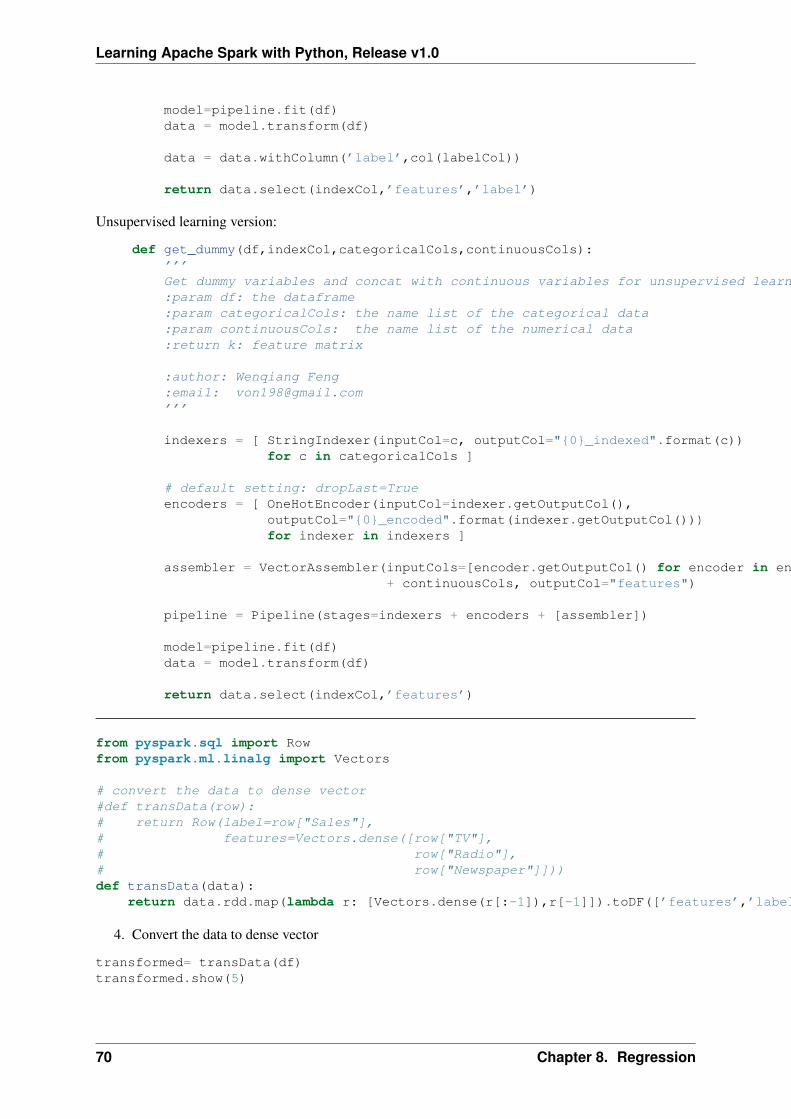
Learning Apache Spark with Python, Release v1.0
model=pipeline.fit(df)data = model.transform(df)
data = data.withColumn(’label’,col(labelCol))
return data.select(indexCol,’features’,’label’)
Unsupervised learning version:
def get_dummy(df,indexCol,categoricalCols,continuousCols):’’’Get dummy variables and concat with continuous variables for unsupervised learning.:param df: the dataframe:param categoricalCols: the name list of the categorical data:param continuousCols: the name list of the numerical data:return k: feature matrix
:author: Wenqiang Feng:email: [email protected]’’’
indexers = [ StringIndexer(inputCol=c, outputCol="{0}_indexed".format(c))for c in categoricalCols ]
# default setting: dropLast=Trueencoders = [ OneHotEncoder(inputCol=indexer.getOutputCol(),
outputCol="{0}_encoded".format(indexer.getOutputCol()))for indexer in indexers ]
assembler = VectorAssembler(inputCols=[encoder.getOutputCol() for encoder in encoders]+ continuousCols, outputCol="features")
pipeline = Pipeline(stages=indexers + encoders + [assembler])
model=pipeline.fit(df)data = model.transform(df)
return data.select(indexCol,’features’)
from pyspark.sql import Rowfrom pyspark.ml.linalg import Vectors
# convert the data to dense vector#def transData(row):# return Row(label=row["Sales"],# features=Vectors.dense([row["TV"],# row["Radio"],# row["Newspaper"]]))def transData(data):
return data.rdd.map(lambda r: [Vectors.dense(r[:-1]),r[-1]]).toDF([’features’,’label’])
4. Convert the data to dense vector
transformed= transData(df)transformed.show(5)
70 Chapter 8. Regression
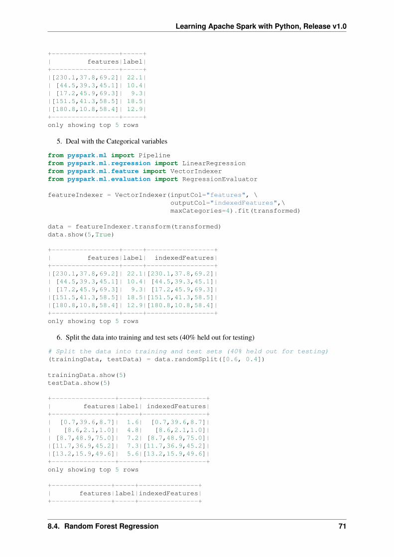
Learning Apache Spark with Python, Release v1.0
+-----------------+-----+| features|label|+-----------------+-----+|[230.1,37.8,69.2]| 22.1|| [44.5,39.3,45.1]| 10.4|| [17.2,45.9,69.3]| 9.3||[151.5,41.3,58.5]| 18.5||[180.8,10.8,58.4]| 12.9|+-----------------+-----+only showing top 5 rows
5. Deal with the Categorical variables
from pyspark.ml import Pipelinefrom pyspark.ml.regression import LinearRegressionfrom pyspark.ml.feature import VectorIndexerfrom pyspark.ml.evaluation import RegressionEvaluator
featureIndexer = VectorIndexer(inputCol="features", \outputCol="indexedFeatures",\maxCategories=4).fit(transformed)
data = featureIndexer.transform(transformed)data.show(5,True)
+-----------------+-----+-----------------+| features|label| indexedFeatures|+-----------------+-----+-----------------+|[230.1,37.8,69.2]| 22.1|[230.1,37.8,69.2]|| [44.5,39.3,45.1]| 10.4| [44.5,39.3,45.1]|| [17.2,45.9,69.3]| 9.3| [17.2,45.9,69.3]||[151.5,41.3,58.5]| 18.5|[151.5,41.3,58.5]||[180.8,10.8,58.4]| 12.9|[180.8,10.8,58.4]|+-----------------+-----+-----------------+only showing top 5 rows
6. Split the data into training and test sets (40% held out for testing)
# Split the data into training and test sets (40% held out for testing)(trainingData, testData) = data.randomSplit([0.6, 0.4])
trainingData.show(5)testData.show(5)
+----------------+-----+----------------+| features|label| indexedFeatures|+----------------+-----+----------------+| [0.7,39.6,8.7]| 1.6| [0.7,39.6,8.7]|| [8.6,2.1,1.0]| 4.8| [8.6,2.1,1.0]|| [8.7,48.9,75.0]| 7.2| [8.7,48.9,75.0]||[11.7,36.9,45.2]| 7.3|[11.7,36.9,45.2]||[13.2,15.9,49.6]| 5.6|[13.2,15.9,49.6]|+----------------+-----+----------------+only showing top 5 rows
+---------------+-----+---------------+| features|label|indexedFeatures|+---------------+-----+---------------+
8.4. Random Forest Regression 71
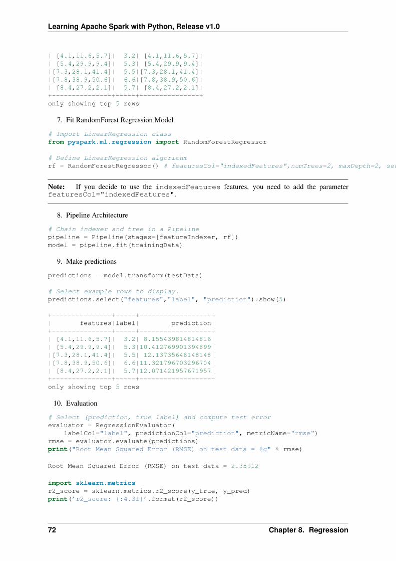
Learning Apache Spark with Python, Release v1.0
| [4.1,11.6,5.7]| 3.2| [4.1,11.6,5.7]|| [5.4,29.9,9.4]| 5.3| [5.4,29.9,9.4]||[7.3,28.1,41.4]| 5.5|[7.3,28.1,41.4]||[7.8,38.9,50.6]| 6.6|[7.8,38.9,50.6]|| [8.4,27.2,2.1]| 5.7| [8.4,27.2,2.1]|+---------------+-----+---------------+only showing top 5 rows
7. Fit RandomForest Regression Model
# Import LinearRegression classfrom pyspark.ml.regression import RandomForestRegressor
# Define LinearRegression algorithmrf = RandomForestRegressor() # featuresCol="indexedFeatures",numTrees=2, maxDepth=2, seed=42
Note: If you decide to use the indexedFeatures features, you need to add the parameterfeaturesCol="indexedFeatures".
8. Pipeline Architecture
# Chain indexer and tree in a Pipelinepipeline = Pipeline(stages=[featureIndexer, rf])model = pipeline.fit(trainingData)
9. Make predictions
predictions = model.transform(testData)
# Select example rows to display.predictions.select("features","label", "prediction").show(5)
+---------------+-----+------------------+| features|label| prediction|+---------------+-----+------------------+| [4.1,11.6,5.7]| 3.2| 8.155439814814816|| [5.4,29.9,9.4]| 5.3|10.412769901394899||[7.3,28.1,41.4]| 5.5| 12.13735648148148||[7.8,38.9,50.6]| 6.6|11.321796703296704|| [8.4,27.2,2.1]| 5.7|12.071421957671957|+---------------+-----+------------------+only showing top 5 rows
10. Evaluation
# Select (prediction, true label) and compute test errorevaluator = RegressionEvaluator(
labelCol="label", predictionCol="prediction", metricName="rmse")rmse = evaluator.evaluate(predictions)print("Root Mean Squared Error (RMSE) on test data = %g" % rmse)
Root Mean Squared Error (RMSE) on test data = 2.35912
import sklearn.metricsr2_score = sklearn.metrics.r2_score(y_true, y_pred)print(’r2_score: {:4.3f}’.format(r2_score))
72 Chapter 8. Regression
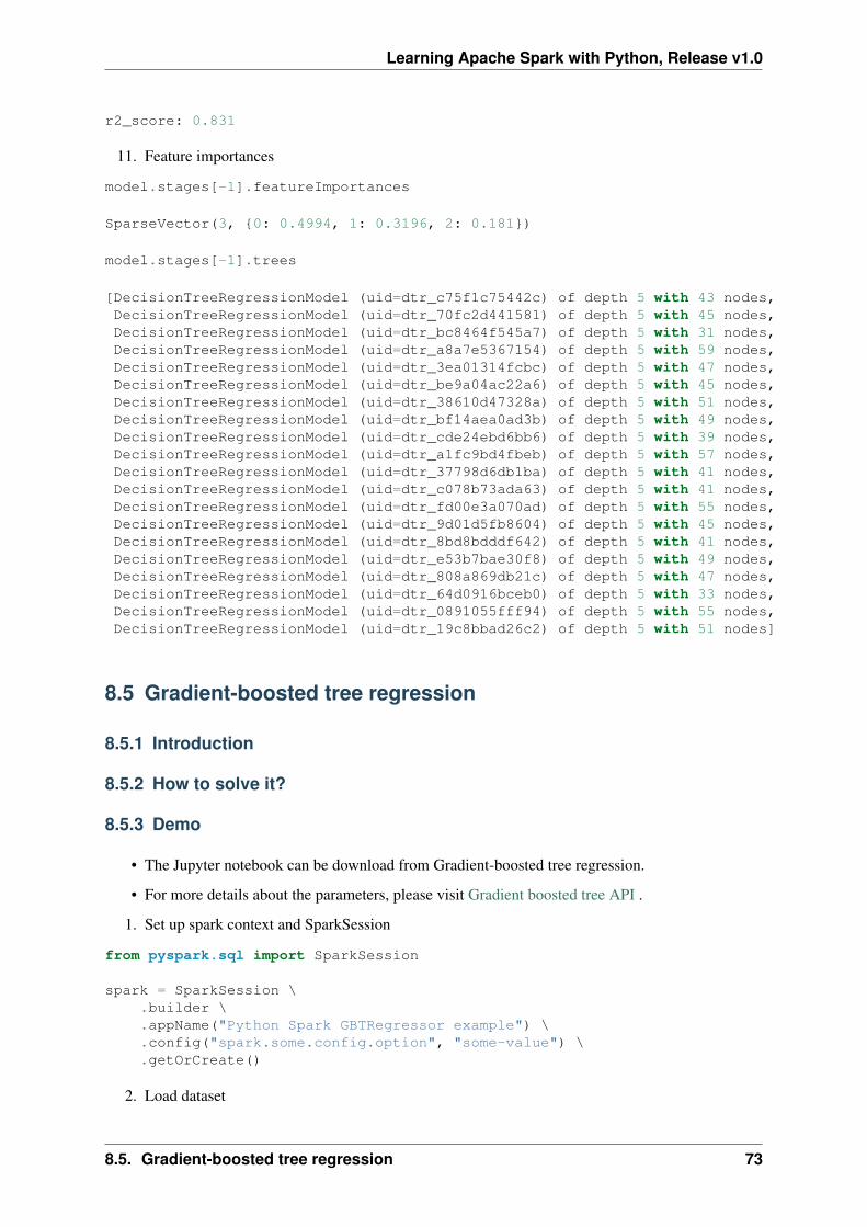
Learning Apache Spark with Python, Release v1.0
r2_score: 0.831
11. Feature importances
model.stages[-1].featureImportances
SparseVector(3, {0: 0.4994, 1: 0.3196, 2: 0.181})
model.stages[-1].trees
[DecisionTreeRegressionModel (uid=dtr_c75f1c75442c) of depth 5 with 43 nodes,DecisionTreeRegressionModel (uid=dtr_70fc2d441581) of depth 5 with 45 nodes,DecisionTreeRegressionModel (uid=dtr_bc8464f545a7) of depth 5 with 31 nodes,DecisionTreeRegressionModel (uid=dtr_a8a7e5367154) of depth 5 with 59 nodes,DecisionTreeRegressionModel (uid=dtr_3ea01314fcbc) of depth 5 with 47 nodes,DecisionTreeRegressionModel (uid=dtr_be9a04ac22a6) of depth 5 with 45 nodes,DecisionTreeRegressionModel (uid=dtr_38610d47328a) of depth 5 with 51 nodes,DecisionTreeRegressionModel (uid=dtr_bf14aea0ad3b) of depth 5 with 49 nodes,DecisionTreeRegressionModel (uid=dtr_cde24ebd6bb6) of depth 5 with 39 nodes,DecisionTreeRegressionModel (uid=dtr_a1fc9bd4fbeb) of depth 5 with 57 nodes,DecisionTreeRegressionModel (uid=dtr_37798d6db1ba) of depth 5 with 41 nodes,DecisionTreeRegressionModel (uid=dtr_c078b73ada63) of depth 5 with 41 nodes,DecisionTreeRegressionModel (uid=dtr_fd00e3a070ad) of depth 5 with 55 nodes,DecisionTreeRegressionModel (uid=dtr_9d01d5fb8604) of depth 5 with 45 nodes,DecisionTreeRegressionModel (uid=dtr_8bd8bdddf642) of depth 5 with 41 nodes,DecisionTreeRegressionModel (uid=dtr_e53b7bae30f8) of depth 5 with 49 nodes,DecisionTreeRegressionModel (uid=dtr_808a869db21c) of depth 5 with 47 nodes,DecisionTreeRegressionModel (uid=dtr_64d0916bceb0) of depth 5 with 33 nodes,DecisionTreeRegressionModel (uid=dtr_0891055fff94) of depth 5 with 55 nodes,DecisionTreeRegressionModel (uid=dtr_19c8bbad26c2) of depth 5 with 51 nodes]
8.5 Gradient-boosted tree regression
8.5.1 Introduction
8.5.2 How to solve it?
8.5.3 Demo
• The Jupyter notebook can be download from Gradient-boosted tree regression.
• For more details about the parameters, please visit Gradient boosted tree API .
1. Set up spark context and SparkSession
from pyspark.sql import SparkSession
spark = SparkSession \.builder \.appName("Python Spark GBTRegressor example") \.config("spark.some.config.option", "some-value") \.getOrCreate()
2. Load dataset
8.5. Gradient-boosted tree regression 73
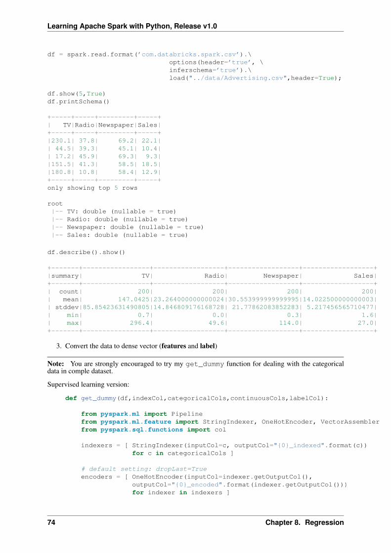
Learning Apache Spark with Python, Release v1.0
df = spark.read.format(’com.databricks.spark.csv’).\options(header=’true’, \inferschema=’true’).\load("../data/Advertising.csv",header=True);
df.show(5,True)df.printSchema()
+-----+-----+---------+-----+| TV|Radio|Newspaper|Sales|+-----+-----+---------+-----+|230.1| 37.8| 69.2| 22.1|| 44.5| 39.3| 45.1| 10.4|| 17.2| 45.9| 69.3| 9.3||151.5| 41.3| 58.5| 18.5||180.8| 10.8| 58.4| 12.9|+-----+-----+---------+-----+only showing top 5 rows
root|-- TV: double (nullable = true)|-- Radio: double (nullable = true)|-- Newspaper: double (nullable = true)|-- Sales: double (nullable = true)
df.describe().show()
+-------+-----------------+------------------+------------------+------------------+|summary| TV| Radio| Newspaper| Sales|+-------+-----------------+------------------+------------------+------------------+| count| 200| 200| 200| 200|| mean| 147.0425|23.264000000000024|30.553999999999995|14.022500000000003|| stddev|85.85423631490805|14.846809176168728| 21.77862083852283| 5.217456565710477|| min| 0.7| 0.0| 0.3| 1.6|| max| 296.4| 49.6| 114.0| 27.0|+-------+-----------------+------------------+------------------+------------------+
3. Convert the data to dense vector (features and label)
Note: You are strongly encouraged to try my get_dummy function for dealing with the categoricaldata in comple dataset.
Supervised learning version:
def get_dummy(df,indexCol,categoricalCols,continuousCols,labelCol):
from pyspark.ml import Pipelinefrom pyspark.ml.feature import StringIndexer, OneHotEncoder, VectorAssemblerfrom pyspark.sql.functions import col
indexers = [ StringIndexer(inputCol=c, outputCol="{0}_indexed".format(c))for c in categoricalCols ]
# default setting: dropLast=Trueencoders = [ OneHotEncoder(inputCol=indexer.getOutputCol(),
outputCol="{0}_encoded".format(indexer.getOutputCol()))for indexer in indexers ]
74 Chapter 8. Regression
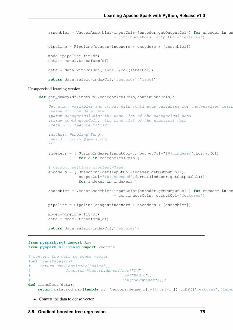
Learning Apache Spark with Python, Release v1.0
assembler = VectorAssembler(inputCols=[encoder.getOutputCol() for encoder in encoders]+ continuousCols, outputCol="features")
pipeline = Pipeline(stages=indexers + encoders + [assembler])
model=pipeline.fit(df)data = model.transform(df)
data = data.withColumn(’label’,col(labelCol))
return data.select(indexCol,’features’,’label’)
Unsupervised learning version:
def get_dummy(df,indexCol,categoricalCols,continuousCols):’’’Get dummy variables and concat with continuous variables for unsupervised learning.:param df: the dataframe:param categoricalCols: the name list of the categorical data:param continuousCols: the name list of the numerical data:return k: feature matrix
:author: Wenqiang Feng:email: [email protected]’’’
indexers = [ StringIndexer(inputCol=c, outputCol="{0}_indexed".format(c))for c in categoricalCols ]
# default setting: dropLast=Trueencoders = [ OneHotEncoder(inputCol=indexer.getOutputCol(),
outputCol="{0}_encoded".format(indexer.getOutputCol()))for indexer in indexers ]
assembler = VectorAssembler(inputCols=[encoder.getOutputCol() for encoder in encoders]+ continuousCols, outputCol="features")
pipeline = Pipeline(stages=indexers + encoders + [assembler])
model=pipeline.fit(df)data = model.transform(df)
return data.select(indexCol,’features’)
from pyspark.sql import Rowfrom pyspark.ml.linalg import Vectors
# convert the data to dense vector#def transData(row):# return Row(label=row["Sales"],# features=Vectors.dense([row["TV"],# row["Radio"],# row["Newspaper"]]))def transData(data):
return data.rdd.map(lambda r: [Vectors.dense(r[:-1]),r[-1]]).toDF([’features’,’label’])
4. Convert the data to dense vector
8.5. Gradient-boosted tree regression 75

Learning Apache Spark with Python, Release v1.0
transformed= transData(df)transformed.show(5)
+-----------------+-----+| features|label|+-----------------+-----+|[230.1,37.8,69.2]| 22.1|| [44.5,39.3,45.1]| 10.4|| [17.2,45.9,69.3]| 9.3||[151.5,41.3,58.5]| 18.5||[180.8,10.8,58.4]| 12.9|+-----------------+-----+only showing top 5 rows
5. Deal with the Categorical variables
from pyspark.ml import Pipelinefrom pyspark.ml.regression import GBTRegressorfrom pyspark.ml.feature import VectorIndexerfrom pyspark.ml.evaluation import RegressionEvaluator
featureIndexer = VectorIndexer(inputCol="features", \outputCol="indexedFeatures",\maxCategories=4).fit(transformed)
data = featureIndexer.transform(transformed)data.show(5,True)
+-----------------+-----+-----------------+| features|label| indexedFeatures|+-----------------+-----+-----------------+|[230.1,37.8,69.2]| 22.1|[230.1,37.8,69.2]|| [44.5,39.3,45.1]| 10.4| [44.5,39.3,45.1]|| [17.2,45.9,69.3]| 9.3| [17.2,45.9,69.3]||[151.5,41.3,58.5]| 18.5|[151.5,41.3,58.5]||[180.8,10.8,58.4]| 12.9|[180.8,10.8,58.4]|+-----------------+-----+-----------------+only showing top 5 rows
6. Split the data into training and test sets (40% held out for testing)
# Split the data into training and test sets (40% held out for testing)(trainingData, testData) = data.randomSplit([0.6, 0.4])
trainingData.show(5)testData.show(5)
+----------------+-----+----------------+| features|label| indexedFeatures|+----------------+-----+----------------+| [0.7,39.6,8.7]| 1.6| [0.7,39.6,8.7]|| [8.6,2.1,1.0]| 4.8| [8.6,2.1,1.0]|| [8.7,48.9,75.0]| 7.2| [8.7,48.9,75.0]||[11.7,36.9,45.2]| 7.3|[11.7,36.9,45.2]||[13.2,15.9,49.6]| 5.6|[13.2,15.9,49.6]|+----------------+-----+----------------+only showing top 5 rows
76 Chapter 8. Regression
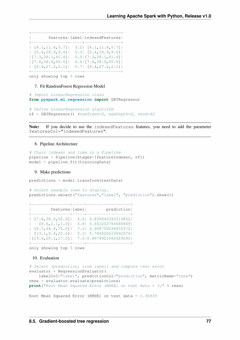
Learning Apache Spark with Python, Release v1.0
+---------------+-----+---------------+| features|label|indexedFeatures|+---------------+-----+---------------+| [4.1,11.6,5.7]| 3.2| [4.1,11.6,5.7]|| [5.4,29.9,9.4]| 5.3| [5.4,29.9,9.4]||[7.3,28.1,41.4]| 5.5|[7.3,28.1,41.4]||[7.8,38.9,50.6]| 6.6|[7.8,38.9,50.6]|| [8.4,27.2,2.1]| 5.7| [8.4,27.2,2.1]|+---------------+-----+---------------+only showing top 5 rows
7. Fit RandomForest Regression Model
# Import LinearRegression classfrom pyspark.ml.regression import GBTRegressor
# Define LinearRegression algorithmrf = GBTRegressor() #numTrees=2, maxDepth=2, seed=42
Note: If you decide to use the indexedFeatures features, you need to add the parameterfeaturesCol="indexedFeatures".
8. Pipeline Architecture
# Chain indexer and tree in a Pipelinepipeline = Pipeline(stages=[featureIndexer, rf])model = pipeline.fit(trainingData)
9. Make predictions
predictions = model.transform(testData)
# Select example rows to display.predictions.select("features","label", "prediction").show(5)
+----------------+-----+------------------+| features|label| prediction|+----------------+-----+------------------+| [7.8,38.9,50.6]| 6.6| 6.836040343319862|| [8.6,2.1,1.0]| 4.8| 5.652202764688849|| [8.7,48.9,75.0]| 7.2| 6.908750296855572|| [13.1,0.4,25.6]| 5.3| 5.784020210692574||[19.6,20.1,17.0]| 7.6|6.8678921062629295|+----------------+-----+------------------+only showing top 5 rows
10. Evaluation
# Select (prediction, true label) and compute test errorevaluator = RegressionEvaluator(
labelCol="label", predictionCol="prediction", metricName="rmse")rmse = evaluator.evaluate(predictions)print("Root Mean Squared Error (RMSE) on test data = %g" % rmse)
Root Mean Squared Error (RMSE) on test data = 1.36939
8.5. Gradient-boosted tree regression 77
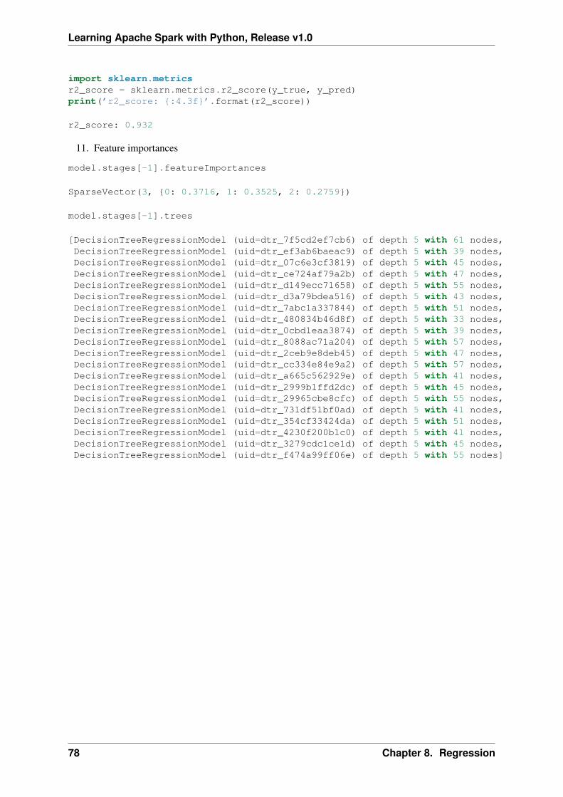
Learning Apache Spark with Python, Release v1.0
import sklearn.metricsr2_score = sklearn.metrics.r2_score(y_true, y_pred)print(’r2_score: {:4.3f}’.format(r2_score))
r2_score: 0.932
11. Feature importances
model.stages[-1].featureImportances
SparseVector(3, {0: 0.3716, 1: 0.3525, 2: 0.2759})
model.stages[-1].trees
[DecisionTreeRegressionModel (uid=dtr_7f5cd2ef7cb6) of depth 5 with 61 nodes,DecisionTreeRegressionModel (uid=dtr_ef3ab6baeac9) of depth 5 with 39 nodes,DecisionTreeRegressionModel (uid=dtr_07c6e3cf3819) of depth 5 with 45 nodes,DecisionTreeRegressionModel (uid=dtr_ce724af79a2b) of depth 5 with 47 nodes,DecisionTreeRegressionModel (uid=dtr_d149ecc71658) of depth 5 with 55 nodes,DecisionTreeRegressionModel (uid=dtr_d3a79bdea516) of depth 5 with 43 nodes,DecisionTreeRegressionModel (uid=dtr_7abc1a337844) of depth 5 with 51 nodes,DecisionTreeRegressionModel (uid=dtr_480834b46d8f) of depth 5 with 33 nodes,DecisionTreeRegressionModel (uid=dtr_0cbd1eaa3874) of depth 5 with 39 nodes,DecisionTreeRegressionModel (uid=dtr_8088ac71a204) of depth 5 with 57 nodes,DecisionTreeRegressionModel (uid=dtr_2ceb9e8deb45) of depth 5 with 47 nodes,DecisionTreeRegressionModel (uid=dtr_cc334e84e9a2) of depth 5 with 57 nodes,DecisionTreeRegressionModel (uid=dtr_a665c562929e) of depth 5 with 41 nodes,DecisionTreeRegressionModel (uid=dtr_2999b1ffd2dc) of depth 5 with 45 nodes,DecisionTreeRegressionModel (uid=dtr_29965cbe8cfc) of depth 5 with 55 nodes,DecisionTreeRegressionModel (uid=dtr_731df51bf0ad) of depth 5 with 41 nodes,DecisionTreeRegressionModel (uid=dtr_354cf33424da) of depth 5 with 51 nodes,DecisionTreeRegressionModel (uid=dtr_4230f200b1c0) of depth 5 with 41 nodes,DecisionTreeRegressionModel (uid=dtr_3279cdc1ce1d) of depth 5 with 45 nodes,DecisionTreeRegressionModel (uid=dtr_f474a99ff06e) of depth 5 with 55 nodes]
78 Chapter 8. Regression
CHAPTER
NINE
REGULARIZATION
In mathematics, statistics, and computer science, particularly in the fields of machine learning and in-verse problems, regularization is a process of introducing additional information in order to solve anill-posed problem or to prevent overfitting (Wikipedia Regularization).
Due to the sparsity within our data, our training sets will often be ill-posed (singular). Applying regu-larization to the regression has many advantages, including:
1. Converting ill-posed problems to well-posed by adding additional information via the penaltyparameter 𝜆
2. Preventing overfitting
3. Variable selection and the removal of correlated variables (Glmnet Vignette). The Ridge methodshrinks the coefficients of correlated variables while the LASSO method picks one variable anddiscards the others. The elastic net penalty is a mixture of these two; if variables are correlatedin groups then 𝛼 = 0.5 tends to select the groups as in or out. If 𝛼 is close to 1, the elastic netperforms much like the LASSO method and removes any degeneracies and wild behavior causedby extreme correlations.
9.1 Ordinary least squares regression
min𝛽∈R𝑝
1
𝑛‖�̂�𝛽 − 𝑌 ‖2
When 𝜆 = 0 (i.e. regParam = 0), then there is no penalty.
LinearRegression(featuresCol="features", labelCol="label", predictionCol="prediction", maxIter=100,regParam=0.0, elasticNetParam=0.0, tol=1e-6, fitIntercept=True, standardization=True, solver="auto",weightCol=None, aggregationDepth=2)
9.2 Ridge regression
min𝛽∈R𝑝
1
𝑛‖�̂�𝛽 − 𝑌 ‖2 + 𝜆‖𝛽‖22
When 𝜆 > 0 (i.e. regParam > 0) and 𝛼 = 0 (i.e. elasticNetParam = 0) , then the penalty is anL2 penalty.
79
Learning Apache Spark with Python, Release v1.0
LinearRegression(featuresCol="features", labelCol="label", predictionCol="prediction", maxIter=100,regParam=0.1, elasticNetParam=0.0, tol=1e-6, fitIntercept=True, standardization=True, solver="auto",weightCol=None, aggregationDepth=2)
9.3 Least Absolute Shrinkage and Selection Operator (LASSO)
min𝛽∈R𝑝
1
𝑛‖�̂�𝛽 − 𝑌 ‖2 + 𝜆‖𝛽‖1
When 𝜆 > 0 (i.e. regParam > 0) and 𝛼 = 1 (i.e. elasticNetParam = 1), then the penalty is anL1 penalty.
LinearRegression(featuresCol="features", labelCol="label", predictionCol="prediction", maxIter=100,regParam=0.0, elasticNetParam=0.0, tol=1e-6, fitIntercept=True, standardization=True, solver="auto",weightCol=None, aggregationDepth=2)
9.4 Elastic net
min𝛽∈R𝑝
1
𝑛‖�̂�𝛽 − 𝑌 ‖2 + 𝜆(𝛼‖𝛽‖1 + (1 − 𝛼)‖𝛽‖22), 𝛼 ∈ (0, 1)
When 𝜆 > 0 (i.e. regParam > 0) and elasticNetParam ∈ (0, 1) (i.e. 𝛼 ∈ (0, 1)) , then thepenalty is an L1 + L2 penalty.
LinearRegression(featuresCol="features", labelCol="label", predictionCol="prediction", maxIter=100,regParam=0.0, elasticNetParam=0.0, tol=1e-6, fitIntercept=True, standardization=True, solver="auto",weightCol=None, aggregationDepth=2)
80 Chapter 9. Regularization
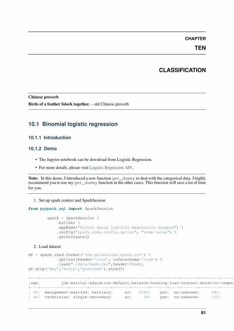
CHAPTER
TEN
CLASSIFICATION
Chinese proverb
Birds of a feather folock together. – old Chinese proverb
10.1 Binomial logistic regression
10.1.1 Introduction
10.1.2 Demo
• The Jupyter notebook can be download from Logistic Regression.
• For more details, please visit Logistic Regression API .
Note: In this demo, I introduced a new function get_dummy to deal with the categorical data. I highlyrecommend you to use my get_dummy function in the other cases. This function will save a lot of timefor you.
1. Set up spark context and SparkSession
from pyspark.sql import SparkSession
spark = SparkSession \.builder \.appName("Python Spark Logistic Regression example") \.config("spark.some.config.option", "some-value") \.getOrCreate()
2. Load dataset
df = spark.read.format(’com.databricks.spark.csv’) \.options(header=’true’, inferschema=’true’) \.load("./data/bank.csv",header=True);
df.drop(’day’,’month’,’poutcome’).show(5)
+---+------------+-------+---------+-------+-------+-------+----+-------+--------+--------+-----+--------+---+|age| job|marital|education|default|balance|housing|loan|contact|duration|campaign|pdays|previous| y|+---+------------+-------+---------+-------+-------+-------+----+-------+--------+--------+-----+--------+---+| 58| management|married| tertiary| no| 2143| yes| no|unknown| 261| 1| -1| 0| no|| 44| technician| single|secondary| no| 29| yes| no|unknown| 151| 1| -1| 0| no|
81
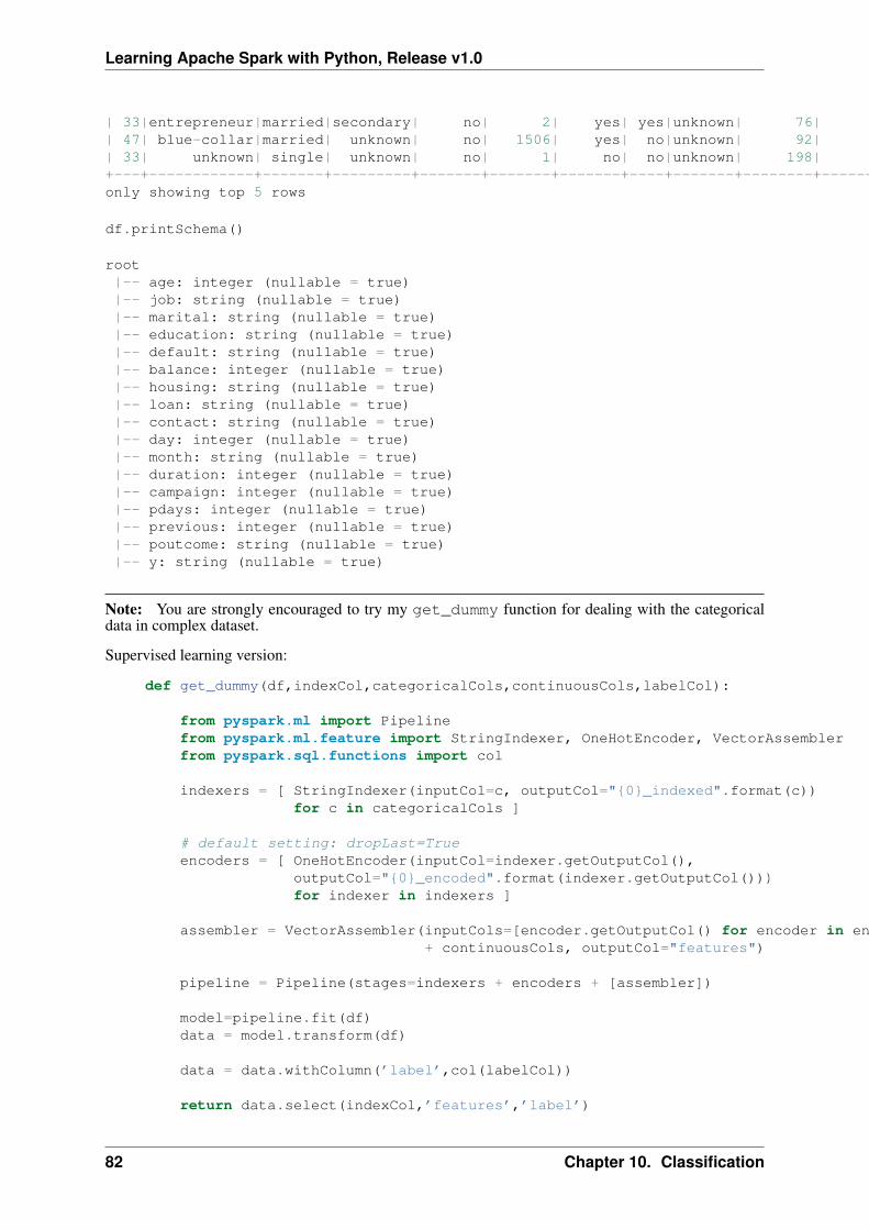
Learning Apache Spark with Python, Release v1.0
| 33|entrepreneur|married|secondary| no| 2| yes| yes|unknown| 76| 1| -1| 0| no|| 47| blue-collar|married| unknown| no| 1506| yes| no|unknown| 92| 1| -1| 0| no|| 33| unknown| single| unknown| no| 1| no| no|unknown| 198| 1| -1| 0| no|+---+------------+-------+---------+-------+-------+-------+----+-------+--------+--------+-----+--------+---+only showing top 5 rows
df.printSchema()
root|-- age: integer (nullable = true)|-- job: string (nullable = true)|-- marital: string (nullable = true)|-- education: string (nullable = true)|-- default: string (nullable = true)|-- balance: integer (nullable = true)|-- housing: string (nullable = true)|-- loan: string (nullable = true)|-- contact: string (nullable = true)|-- day: integer (nullable = true)|-- month: string (nullable = true)|-- duration: integer (nullable = true)|-- campaign: integer (nullable = true)|-- pdays: integer (nullable = true)|-- previous: integer (nullable = true)|-- poutcome: string (nullable = true)|-- y: string (nullable = true)
Note: You are strongly encouraged to try my get_dummy function for dealing with the categoricaldata in complex dataset.
Supervised learning version:
def get_dummy(df,indexCol,categoricalCols,continuousCols,labelCol):
from pyspark.ml import Pipelinefrom pyspark.ml.feature import StringIndexer, OneHotEncoder, VectorAssemblerfrom pyspark.sql.functions import col
indexers = [ StringIndexer(inputCol=c, outputCol="{0}_indexed".format(c))for c in categoricalCols ]
# default setting: dropLast=Trueencoders = [ OneHotEncoder(inputCol=indexer.getOutputCol(),
outputCol="{0}_encoded".format(indexer.getOutputCol()))for indexer in indexers ]
assembler = VectorAssembler(inputCols=[encoder.getOutputCol() for encoder in encoders]+ continuousCols, outputCol="features")
pipeline = Pipeline(stages=indexers + encoders + [assembler])
model=pipeline.fit(df)data = model.transform(df)
data = data.withColumn(’label’,col(labelCol))
return data.select(indexCol,’features’,’label’)
82 Chapter 10. Classification
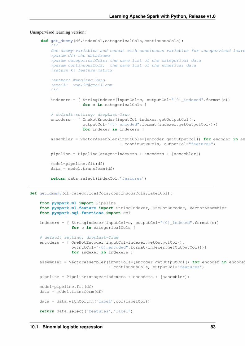
Learning Apache Spark with Python, Release v1.0
Unsupervised learning version:
def get_dummy(df,indexCol,categoricalCols,continuousCols):’’’Get dummy variables and concat with continuous variables for unsupervised learning.:param df: the dataframe:param categoricalCols: the name list of the categorical data:param continuousCols: the name list of the numerical data:return k: feature matrix
:author: Wenqiang Feng:email: [email protected]’’’
indexers = [ StringIndexer(inputCol=c, outputCol="{0}_indexed".format(c))for c in categoricalCols ]
# default setting: dropLast=Trueencoders = [ OneHotEncoder(inputCol=indexer.getOutputCol(),
outputCol="{0}_encoded".format(indexer.getOutputCol()))for indexer in indexers ]
assembler = VectorAssembler(inputCols=[encoder.getOutputCol() for encoder in encoders]+ continuousCols, outputCol="features")
pipeline = Pipeline(stages=indexers + encoders + [assembler])
model=pipeline.fit(df)data = model.transform(df)
return data.select(indexCol,’features’)
def get_dummy(df,categoricalCols,continuousCols,labelCol):
from pyspark.ml import Pipelinefrom pyspark.ml.feature import StringIndexer, OneHotEncoder, VectorAssemblerfrom pyspark.sql.functions import col
indexers = [ StringIndexer(inputCol=c, outputCol="{0}_indexed".format(c))for c in categoricalCols ]
# default setting: dropLast=Trueencoders = [ OneHotEncoder(inputCol=indexer.getOutputCol(),
outputCol="{0}_encoded".format(indexer.getOutputCol()))for indexer in indexers ]
assembler = VectorAssembler(inputCols=[encoder.getOutputCol() for encoder in encoders]+ continuousCols, outputCol="features")
pipeline = Pipeline(stages=indexers + encoders + [assembler])
model=pipeline.fit(df)data = model.transform(df)
data = data.withColumn(’label’,col(labelCol))
return data.select(’features’,’label’)
10.1. Binomial logistic regression 83
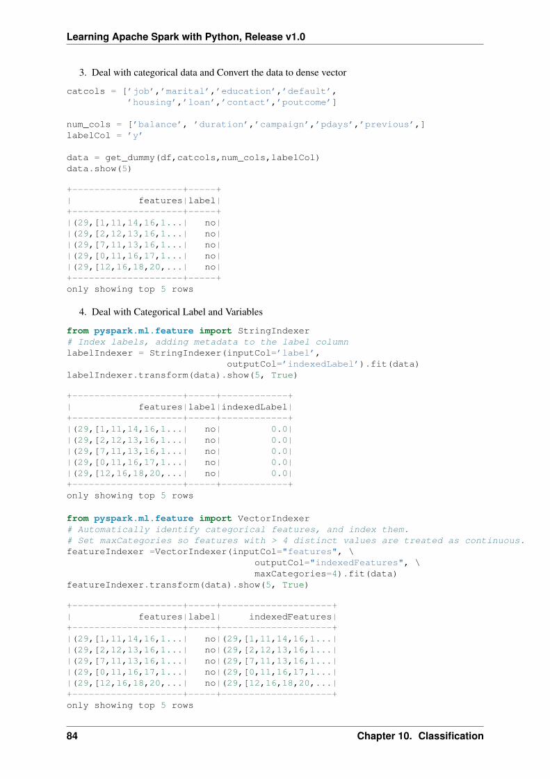
Learning Apache Spark with Python, Release v1.0
3. Deal with categorical data and Convert the data to dense vector
catcols = [’job’,’marital’,’education’,’default’,’housing’,’loan’,’contact’,’poutcome’]
num_cols = [’balance’, ’duration’,’campaign’,’pdays’,’previous’,]labelCol = ’y’
data = get_dummy(df,catcols,num_cols,labelCol)data.show(5)
+--------------------+-----+| features|label|+--------------------+-----+|(29,[1,11,14,16,1...| no||(29,[2,12,13,16,1...| no||(29,[7,11,13,16,1...| no||(29,[0,11,16,17,1...| no||(29,[12,16,18,20,...| no|+--------------------+-----+only showing top 5 rows
4. Deal with Categorical Label and Variables
from pyspark.ml.feature import StringIndexer# Index labels, adding metadata to the label columnlabelIndexer = StringIndexer(inputCol=’label’,
outputCol=’indexedLabel’).fit(data)labelIndexer.transform(data).show(5, True)
+--------------------+-----+------------+| features|label|indexedLabel|+--------------------+-----+------------+|(29,[1,11,14,16,1...| no| 0.0||(29,[2,12,13,16,1...| no| 0.0||(29,[7,11,13,16,1...| no| 0.0||(29,[0,11,16,17,1...| no| 0.0||(29,[12,16,18,20,...| no| 0.0|+--------------------+-----+------------+only showing top 5 rows
from pyspark.ml.feature import VectorIndexer# Automatically identify categorical features, and index them.# Set maxCategories so features with > 4 distinct values are treated as continuous.featureIndexer =VectorIndexer(inputCol="features", \
outputCol="indexedFeatures", \maxCategories=4).fit(data)
featureIndexer.transform(data).show(5, True)
+--------------------+-----+--------------------+| features|label| indexedFeatures|+--------------------+-----+--------------------+|(29,[1,11,14,16,1...| no|(29,[1,11,14,16,1...||(29,[2,12,13,16,1...| no|(29,[2,12,13,16,1...||(29,[7,11,13,16,1...| no|(29,[7,11,13,16,1...||(29,[0,11,16,17,1...| no|(29,[0,11,16,17,1...||(29,[12,16,18,20,...| no|(29,[12,16,18,20,...|+--------------------+-----+--------------------+only showing top 5 rows
84 Chapter 10. Classification
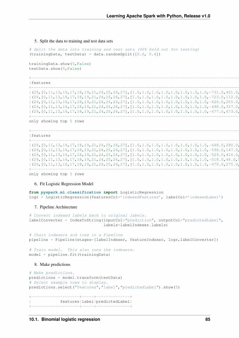
Learning Apache Spark with Python, Release v1.0
5. Split the data to training and test data sets
# Split the data into training and test sets (40% held out for testing)(trainingData, testData) = data.randomSplit([0.6, 0.4])
trainingData.show(5,False)testData.show(5,False)
+-------------------------------------------------------------------------------------------------+-----+|features |label|+-------------------------------------------------------------------------------------------------+-----+|(29,[0,11,13,16,17,18,19,21,24,25,26,27],[1.0,1.0,1.0,1.0,1.0,1.0,1.0,1.0,-731.0,401.0,4.0,-1.0])|no ||(29,[0,11,13,16,17,18,19,21,24,25,26,27],[1.0,1.0,1.0,1.0,1.0,1.0,1.0,1.0,-723.0,112.0,2.0,-1.0])|no ||(29,[0,11,13,16,17,18,19,21,24,25,26,27],[1.0,1.0,1.0,1.0,1.0,1.0,1.0,1.0,-626.0,205.0,1.0,-1.0])|no ||(29,[0,11,13,16,17,18,19,21,24,25,26,27],[1.0,1.0,1.0,1.0,1.0,1.0,1.0,1.0,-498.0,357.0,1.0,-1.0])|no ||(29,[0,11,13,16,17,18,19,21,24,25,26,27],[1.0,1.0,1.0,1.0,1.0,1.0,1.0,1.0,-477.0,473.0,2.0,-1.0])|no |+-------------------------------------------------------------------------------------------------+-----+only showing top 5 rows
+-------------------------------------------------------------------------------------------------+-----+|features |label|+-------------------------------------------------------------------------------------------------+-----+|(29,[0,11,13,16,17,18,19,21,24,25,26,27],[1.0,1.0,1.0,1.0,1.0,1.0,1.0,1.0,-648.0,280.0,2.0,-1.0])|no ||(29,[0,11,13,16,17,18,19,21,24,25,26,27],[1.0,1.0,1.0,1.0,1.0,1.0,1.0,1.0,-596.0,147.0,1.0,-1.0])|no ||(29,[0,11,13,16,17,18,19,21,24,25,26,27],[1.0,1.0,1.0,1.0,1.0,1.0,1.0,1.0,-529.0,416.0,4.0,-1.0])|no ||(29,[0,11,13,16,17,18,19,21,24,25,26,27],[1.0,1.0,1.0,1.0,1.0,1.0,1.0,1.0,-518.0,46.0,5.0,-1.0]) |no ||(29,[0,11,13,16,17,18,19,21,24,25,26,27],[1.0,1.0,1.0,1.0,1.0,1.0,1.0,1.0,-470.0,275.0,2.0,-1.0])|no |+-------------------------------------------------------------------------------------------------+-----+only showing top 5 rows
6. Fit Logistic Regression Model
from pyspark.ml.classification import LogisticRegressionlogr = LogisticRegression(featuresCol=’indexedFeatures’, labelCol=’indexedLabel’)
7. Pipeline Architecture
# Convert indexed labels back to original labels.labelConverter = IndexToString(inputCol="prediction", outputCol="predictedLabel",
labels=labelIndexer.labels)
# Chain indexers and tree in a Pipelinepipeline = Pipeline(stages=[labelIndexer, featureIndexer, logr,labelConverter])
# Train model. This also runs the indexers.model = pipeline.fit(trainingData)
8. Make predictions
# Make predictions.predictions = model.transform(testData)# Select example rows to display.predictions.select("features","label","predictedLabel").show(5)
+--------------------+-----+--------------+| features|label|predictedLabel|+--------------------+-----+--------------+
10.1. Binomial logistic regression 85
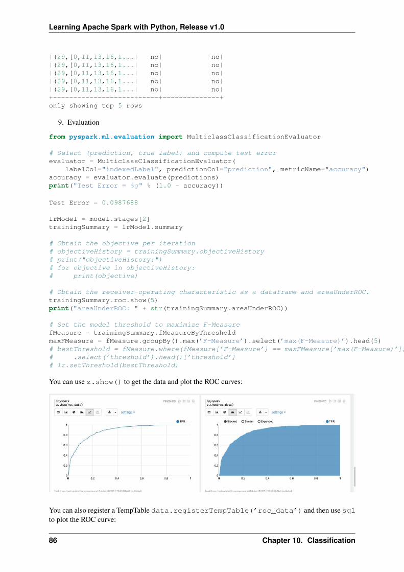
Learning Apache Spark with Python, Release v1.0
|(29,[0,11,13,16,1...| no| no||(29,[0,11,13,16,1...| no| no||(29,[0,11,13,16,1...| no| no||(29,[0,11,13,16,1...| no| no||(29,[0,11,13,16,1...| no| no|+--------------------+-----+--------------+only showing top 5 rows
9. Evaluation
from pyspark.ml.evaluation import MulticlassClassificationEvaluator
# Select (prediction, true label) and compute test errorevaluator = MulticlassClassificationEvaluator(
labelCol="indexedLabel", predictionCol="prediction", metricName="accuracy")accuracy = evaluator.evaluate(predictions)print("Test Error = %g" % (1.0 - accuracy))
Test Error = 0.0987688
lrModel = model.stages[2]trainingSummary = lrModel.summary
# Obtain the objective per iteration# objectiveHistory = trainingSummary.objectiveHistory# print("objectiveHistory:")# for objective in objectiveHistory:# print(objective)
# Obtain the receiver-operating characteristic as a dataframe and areaUnderROC.trainingSummary.roc.show(5)print("areaUnderROC: " + str(trainingSummary.areaUnderROC))
# Set the model threshold to maximize F-MeasurefMeasure = trainingSummary.fMeasureByThresholdmaxFMeasure = fMeasure.groupBy().max(’F-Measure’).select(’max(F-Measure)’).head(5)# bestThreshold = fMeasure.where(fMeasure[’F-Measure’] == maxFMeasure[’max(F-Measure)’]) \# .select(’threshold’).head()[’threshold’]# lr.setThreshold(bestThreshold)
You can use z.show() to get the data and plot the ROC curves:
You can also register a TempTable data.registerTempTable(’roc_data’) and then use sqlto plot the ROC curve:
86 Chapter 10. Classification
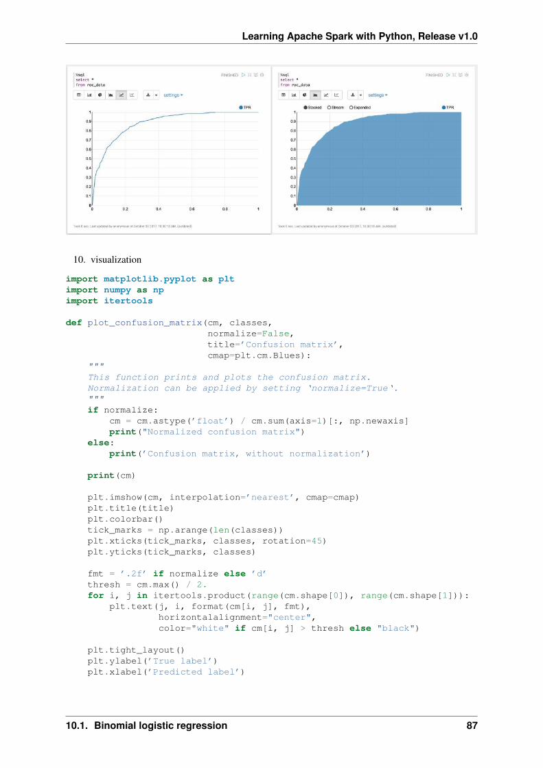
Learning Apache Spark with Python, Release v1.0
10. visualization
import matplotlib.pyplot as pltimport numpy as npimport itertools
def plot_confusion_matrix(cm, classes,normalize=False,title=’Confusion matrix’,cmap=plt.cm.Blues):
"""This function prints and plots the confusion matrix.Normalization can be applied by setting ‘normalize=True‘."""if normalize:
cm = cm.astype(’float’) / cm.sum(axis=1)[:, np.newaxis]print("Normalized confusion matrix")
else:print(’Confusion matrix, without normalization’)
print(cm)
plt.imshow(cm, interpolation=’nearest’, cmap=cmap)plt.title(title)plt.colorbar()tick_marks = np.arange(len(classes))plt.xticks(tick_marks, classes, rotation=45)plt.yticks(tick_marks, classes)
fmt = ’.2f’ if normalize else ’d’thresh = cm.max() / 2.for i, j in itertools.product(range(cm.shape[0]), range(cm.shape[1])):
plt.text(j, i, format(cm[i, j], fmt),horizontalalignment="center",color="white" if cm[i, j] > thresh else "black")
plt.tight_layout()plt.ylabel(’True label’)plt.xlabel(’Predicted label’)
10.1. Binomial logistic regression 87
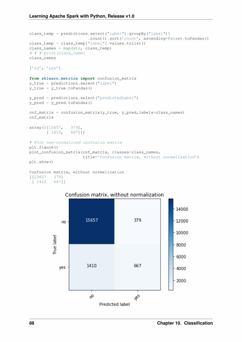
Learning Apache Spark with Python, Release v1.0
class_temp = predictions.select("label").groupBy("label")\.count().sort(’count’, ascending=False).toPandas()
class_temp = class_temp["label"].values.tolist()class_names = map(str, class_temp)# # # print(class_name)class_names
[’no’, ’yes’]
from sklearn.metrics import confusion_matrixy_true = predictions.select("label")y_true = y_true.toPandas()
y_pred = predictions.select("predictedLabel")y_pred = y_pred.toPandas()
cnf_matrix = confusion_matrix(y_true, y_pred,labels=class_names)cnf_matrix
array([[15657, 379],[ 1410, 667]])
# Plot non-normalized confusion matrixplt.figure()plot_confusion_matrix(cnf_matrix, classes=class_names,
title=’Confusion matrix, without normalization’)plt.show()
Confusion matrix, without normalization[[15657 379][ 1410 667]]
88 Chapter 10. Classification
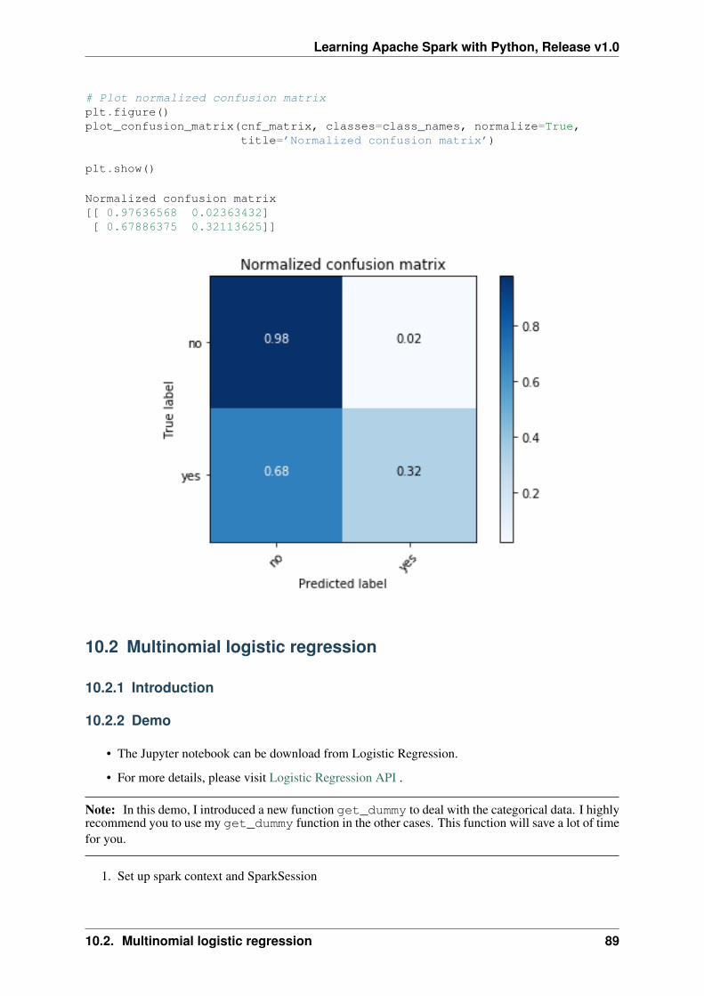
Learning Apache Spark with Python, Release v1.0
# Plot normalized confusion matrixplt.figure()plot_confusion_matrix(cnf_matrix, classes=class_names, normalize=True,
title=’Normalized confusion matrix’)
plt.show()
Normalized confusion matrix[[ 0.97636568 0.02363432][ 0.67886375 0.32113625]]
10.2 Multinomial logistic regression
10.2.1 Introduction
10.2.2 Demo
• The Jupyter notebook can be download from Logistic Regression.
• For more details, please visit Logistic Regression API .
Note: In this demo, I introduced a new function get_dummy to deal with the categorical data. I highlyrecommend you to use my get_dummy function in the other cases. This function will save a lot of timefor you.
1. Set up spark context and SparkSession
10.2. Multinomial logistic regression 89
Learning Apache Spark with Python, Release v1.0
from pyspark.sql import SparkSession
spark = SparkSession \.builder \.appName("Python Spark MultinomialLogisticRegression classification") \.config("spark.some.config.option", "some-value") \.getOrCreate()
2. Load dataset
df = spark.read.format(’com.databricks.spark.csv’) \.options(header=’true’, inferschema=’true’) \.load("./data/WineData2.csv",header=True);
df.show(5)
+-----+--------+------+-----+---------+----+-----+-------+----+---------+-------+-------+|fixed|volatile|citric|sugar|chlorides|free|total|density| pH|sulphates|alcohol|quality|+-----+--------+------+-----+---------+----+-----+-------+----+---------+-------+-------+| 7.4| 0.7| 0.0| 1.9| 0.076|11.0| 34.0| 0.9978|3.51| 0.56| 9.4| 5|| 7.8| 0.88| 0.0| 2.6| 0.098|25.0| 67.0| 0.9968| 3.2| 0.68| 9.8| 5|| 7.8| 0.76| 0.04| 2.3| 0.092|15.0| 54.0| 0.997|3.26| 0.65| 9.8| 5|| 11.2| 0.28| 0.56| 1.9| 0.075|17.0| 60.0| 0.998|3.16| 0.58| 9.8| 6|| 7.4| 0.7| 0.0| 1.9| 0.076|11.0| 34.0| 0.9978|3.51| 0.56| 9.4| 5|+-----+--------+------+-----+---------+----+-----+-------+----+---------+-------+-------+only showing top 5 rows
df.printSchema()
root|-- fixed: double (nullable = true)|-- volatile: double (nullable = true)|-- citric: double (nullable = true)|-- sugar: double (nullable = true)|-- chlorides: double (nullable = true)|-- free: double (nullable = true)|-- total: double (nullable = true)|-- density: double (nullable = true)|-- pH: double (nullable = true)|-- sulphates: double (nullable = true)|-- alcohol: double (nullable = true)|-- quality: string (nullable = true)
# Convert to float formatdef string_to_float(x):
return float(x)
#def condition(r):
if (0<= r <= 4):label = "low"
elif(4< r <= 6):label = "medium"
else:label = "high"
return label
from pyspark.sql.functions import udffrom pyspark.sql.types import StringType, DoubleType
90 Chapter 10. Classification

Learning Apache Spark with Python, Release v1.0
string_to_float_udf = udf(string_to_float, DoubleType())quality_udf = udf(lambda x: condition(x), StringType())
df = df.withColumn("quality", quality_udf("quality"))
df.show(5,True)
+-----+--------+------+-----+---------+----+-----+-------+----+---------+-------+-------+|fixed|volatile|citric|sugar|chlorides|free|total|density| pH|sulphates|alcohol|quality|+-----+--------+------+-----+---------+----+-----+-------+----+---------+-------+-------+| 7.4| 0.7| 0.0| 1.9| 0.076|11.0| 34.0| 0.9978|3.51| 0.56| 9.4| medium|| 7.8| 0.88| 0.0| 2.6| 0.098|25.0| 67.0| 0.9968| 3.2| 0.68| 9.8| medium|| 7.8| 0.76| 0.04| 2.3| 0.092|15.0| 54.0| 0.997|3.26| 0.65| 9.8| medium|| 11.2| 0.28| 0.56| 1.9| 0.075|17.0| 60.0| 0.998|3.16| 0.58| 9.8| medium|| 7.4| 0.7| 0.0| 1.9| 0.076|11.0| 34.0| 0.9978|3.51| 0.56| 9.4| medium|+-----+--------+------+-----+---------+----+-----+-------+----+---------+-------+-------+only showing top 5 rows
df.printSchema()
root|-- fixed: double (nullable = true)|-- volatile: double (nullable = true)|-- citric: double (nullable = true)|-- sugar: double (nullable = true)|-- chlorides: double (nullable = true)|-- free: double (nullable = true)|-- total: double (nullable = true)|-- density: double (nullable = true)|-- pH: double (nullable = true)|-- sulphates: double (nullable = true)|-- alcohol: double (nullable = true)|-- quality: string (nullable = true)
3. Deal with categorical data and Convert the data to dense vector
Note: You are strongly encouraged to try my get_dummy function for dealing with the categoricaldata in complex dataset.
Supervised learning version:
def get_dummy(df,indexCol,categoricalCols,continuousCols,labelCol):
from pyspark.ml import Pipelinefrom pyspark.ml.feature import StringIndexer, OneHotEncoder, VectorAssemblerfrom pyspark.sql.functions import col
indexers = [ StringIndexer(inputCol=c, outputCol="{0}_indexed".format(c))for c in categoricalCols ]
# default setting: dropLast=Trueencoders = [ OneHotEncoder(inputCol=indexer.getOutputCol(),
outputCol="{0}_encoded".format(indexer.getOutputCol()))for indexer in indexers ]
assembler = VectorAssembler(inputCols=[encoder.getOutputCol() for encoder in encoders]+ continuousCols, outputCol="features")
10.2. Multinomial logistic regression 91
Learning Apache Spark with Python, Release v1.0
pipeline = Pipeline(stages=indexers + encoders + [assembler])
model=pipeline.fit(df)data = model.transform(df)
data = data.withColumn(’label’,col(labelCol))
return data.select(indexCol,’features’,’label’)
Unsupervised learning version:
def get_dummy(df,indexCol,categoricalCols,continuousCols):’’’Get dummy variables and concat with continuous variables for unsupervised learning.:param df: the dataframe:param categoricalCols: the name list of the categorical data:param continuousCols: the name list of the numerical data:return k: feature matrix
:author: Wenqiang Feng:email: [email protected]’’’
indexers = [ StringIndexer(inputCol=c, outputCol="{0}_indexed".format(c))for c in categoricalCols ]
# default setting: dropLast=Trueencoders = [ OneHotEncoder(inputCol=indexer.getOutputCol(),
outputCol="{0}_encoded".format(indexer.getOutputCol()))for indexer in indexers ]
assembler = VectorAssembler(inputCols=[encoder.getOutputCol() for encoder in encoders]+ continuousCols, outputCol="features")
pipeline = Pipeline(stages=indexers + encoders + [assembler])
model=pipeline.fit(df)data = model.transform(df)
return data.select(indexCol,’features’)
def get_dummy(df,categoricalCols,continuousCols,labelCol):
from pyspark.ml import Pipelinefrom pyspark.ml.feature import StringIndexer, OneHotEncoder, VectorAssemblerfrom pyspark.sql.functions import col
indexers = [ StringIndexer(inputCol=c, outputCol="{0}_indexed".format(c))for c in categoricalCols ]
# default setting: dropLast=Trueencoders = [ OneHotEncoder(inputCol=indexer.getOutputCol(),
outputCol="{0}_encoded".format(indexer.getOutputCol()))for indexer in indexers ]
assembler = VectorAssembler(inputCols=[encoder.getOutputCol() for encoder in encoders]+ continuousCols, outputCol="features")
92 Chapter 10. Classification
Learning Apache Spark with Python, Release v1.0
pipeline = Pipeline(stages=indexers + encoders + [assembler])
model=pipeline.fit(df)data = model.transform(df)
data = data.withColumn(’label’,col(labelCol))
return data.select(’features’,’label’)
4. Transform the dataset to DataFrame
from pyspark.ml.linalg import Vectors # !!!!caution: not from pyspark.mllib.linalg import Vectorsfrom pyspark.ml import Pipelinefrom pyspark.ml.feature import IndexToString,StringIndexer, VectorIndexerfrom pyspark.ml.tuning import CrossValidator, ParamGridBuilderfrom pyspark.ml.evaluation import MulticlassClassificationEvaluator
def transData(data):return data.rdd.map(lambda r: [Vectors.dense(r[:-1]),r[-1]]).toDF([’features’,’label’])
transformed = transData(df)transformed.show(5)
+--------------------+------+| features| label|+--------------------+------+|[7.4,0.7,0.0,1.9,...|medium||[7.8,0.88,0.0,2.6...|medium||[7.8,0.76,0.04,2....|medium||[11.2,0.28,0.56,1...|medium||[7.4,0.7,0.0,1.9,...|medium|+--------------------+------+only showing top 5 rows
4. Deal with Categorical Label and Variables
# Index labels, adding metadata to the label columnlabelIndexer = StringIndexer(inputCol=’label’,
outputCol=’indexedLabel’).fit(transformed)labelIndexer.transform(transformed).show(5, True)
+--------------------+------+------------+| features| label|indexedLabel|+--------------------+------+------------+|[7.4,0.7,0.0,1.9,...|medium| 0.0||[7.8,0.88,0.0,2.6...|medium| 0.0||[7.8,0.76,0.04,2....|medium| 0.0||[11.2,0.28,0.56,1...|medium| 0.0||[7.4,0.7,0.0,1.9,...|medium| 0.0|+--------------------+------+------------+only showing top 5 rows
# Automatically identify categorical features, and index them.# Set maxCategories so features with > 4 distinct values are treated as continuous.featureIndexer =VectorIndexer(inputCol="features", \
outputCol="indexedFeatures", \maxCategories=4).fit(transformed)
featureIndexer.transform(transformed).show(5, True)
10.2. Multinomial logistic regression 93
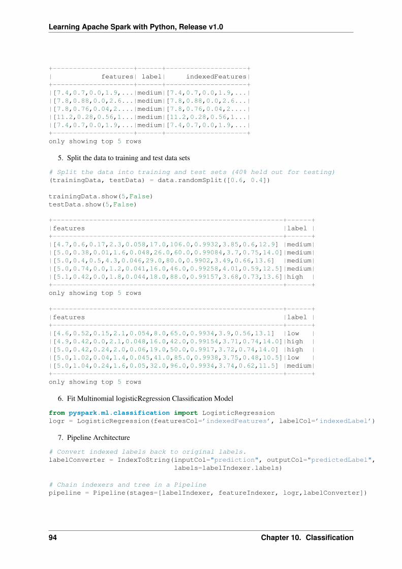
Learning Apache Spark with Python, Release v1.0
+--------------------+------+--------------------+| features| label| indexedFeatures|+--------------------+------+--------------------+|[7.4,0.7,0.0,1.9,...|medium|[7.4,0.7,0.0,1.9,...||[7.8,0.88,0.0,2.6...|medium|[7.8,0.88,0.0,2.6...||[7.8,0.76,0.04,2....|medium|[7.8,0.76,0.04,2....||[11.2,0.28,0.56,1...|medium|[11.2,0.28,0.56,1...||[7.4,0.7,0.0,1.9,...|medium|[7.4,0.7,0.0,1.9,...|+--------------------+------+--------------------+only showing top 5 rows
5. Split the data to training and test data sets
# Split the data into training and test sets (40% held out for testing)(trainingData, testData) = data.randomSplit([0.6, 0.4])
trainingData.show(5,False)testData.show(5,False)
+---------------------------------------------------------+------+|features |label |+---------------------------------------------------------+------+|[4.7,0.6,0.17,2.3,0.058,17.0,106.0,0.9932,3.85,0.6,12.9] |medium||[5.0,0.38,0.01,1.6,0.048,26.0,60.0,0.99084,3.7,0.75,14.0]|medium||[5.0,0.4,0.5,4.3,0.046,29.0,80.0,0.9902,3.49,0.66,13.6] |medium||[5.0,0.74,0.0,1.2,0.041,16.0,46.0,0.99258,4.01,0.59,12.5]|medium||[5.1,0.42,0.0,1.8,0.044,18.0,88.0,0.99157,3.68,0.73,13.6]|high |+---------------------------------------------------------+------+only showing top 5 rows
+---------------------------------------------------------+------+|features |label |+---------------------------------------------------------+------+|[4.6,0.52,0.15,2.1,0.054,8.0,65.0,0.9934,3.9,0.56,13.1] |low ||[4.9,0.42,0.0,2.1,0.048,16.0,42.0,0.99154,3.71,0.74,14.0]|high ||[5.0,0.42,0.24,2.0,0.06,19.0,50.0,0.9917,3.72,0.74,14.0] |high ||[5.0,1.02,0.04,1.4,0.045,41.0,85.0,0.9938,3.75,0.48,10.5]|low ||[5.0,1.04,0.24,1.6,0.05,32.0,96.0,0.9934,3.74,0.62,11.5] |medium|+---------------------------------------------------------+------+only showing top 5 rows
6. Fit Multinomial logisticRegression Classification Model
from pyspark.ml.classification import LogisticRegressionlogr = LogisticRegression(featuresCol=’indexedFeatures’, labelCol=’indexedLabel’)
7. Pipeline Architecture
# Convert indexed labels back to original labels.labelConverter = IndexToString(inputCol="prediction", outputCol="predictedLabel",
labels=labelIndexer.labels)
# Chain indexers and tree in a Pipelinepipeline = Pipeline(stages=[labelIndexer, featureIndexer, logr,labelConverter])
94 Chapter 10. Classification
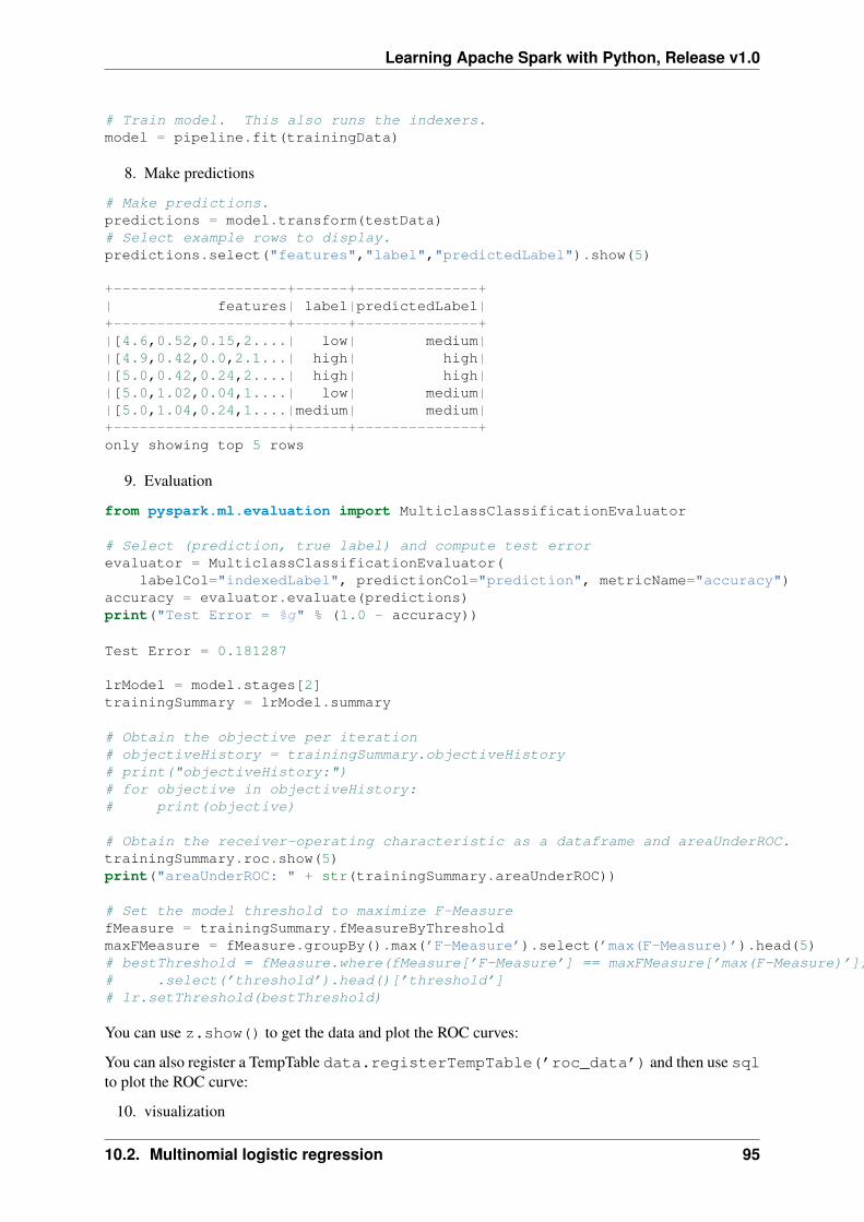
Learning Apache Spark with Python, Release v1.0
# Train model. This also runs the indexers.model = pipeline.fit(trainingData)
8. Make predictions
# Make predictions.predictions = model.transform(testData)# Select example rows to display.predictions.select("features","label","predictedLabel").show(5)
+--------------------+------+--------------+| features| label|predictedLabel|+--------------------+------+--------------+|[4.6,0.52,0.15,2....| low| medium||[4.9,0.42,0.0,2.1...| high| high||[5.0,0.42,0.24,2....| high| high||[5.0,1.02,0.04,1....| low| medium||[5.0,1.04,0.24,1....|medium| medium|+--------------------+------+--------------+only showing top 5 rows
9. Evaluation
from pyspark.ml.evaluation import MulticlassClassificationEvaluator
# Select (prediction, true label) and compute test errorevaluator = MulticlassClassificationEvaluator(
labelCol="indexedLabel", predictionCol="prediction", metricName="accuracy")accuracy = evaluator.evaluate(predictions)print("Test Error = %g" % (1.0 - accuracy))
Test Error = 0.181287
lrModel = model.stages[2]trainingSummary = lrModel.summary
# Obtain the objective per iteration# objectiveHistory = trainingSummary.objectiveHistory# print("objectiveHistory:")# for objective in objectiveHistory:# print(objective)
# Obtain the receiver-operating characteristic as a dataframe and areaUnderROC.trainingSummary.roc.show(5)print("areaUnderROC: " + str(trainingSummary.areaUnderROC))
# Set the model threshold to maximize F-MeasurefMeasure = trainingSummary.fMeasureByThresholdmaxFMeasure = fMeasure.groupBy().max(’F-Measure’).select(’max(F-Measure)’).head(5)# bestThreshold = fMeasure.where(fMeasure[’F-Measure’] == maxFMeasure[’max(F-Measure)’]) \# .select(’threshold’).head()[’threshold’]# lr.setThreshold(bestThreshold)
You can use z.show() to get the data and plot the ROC curves:
You can also register a TempTable data.registerTempTable(’roc_data’) and then use sqlto plot the ROC curve:
10. visualization
10.2. Multinomial logistic regression 95
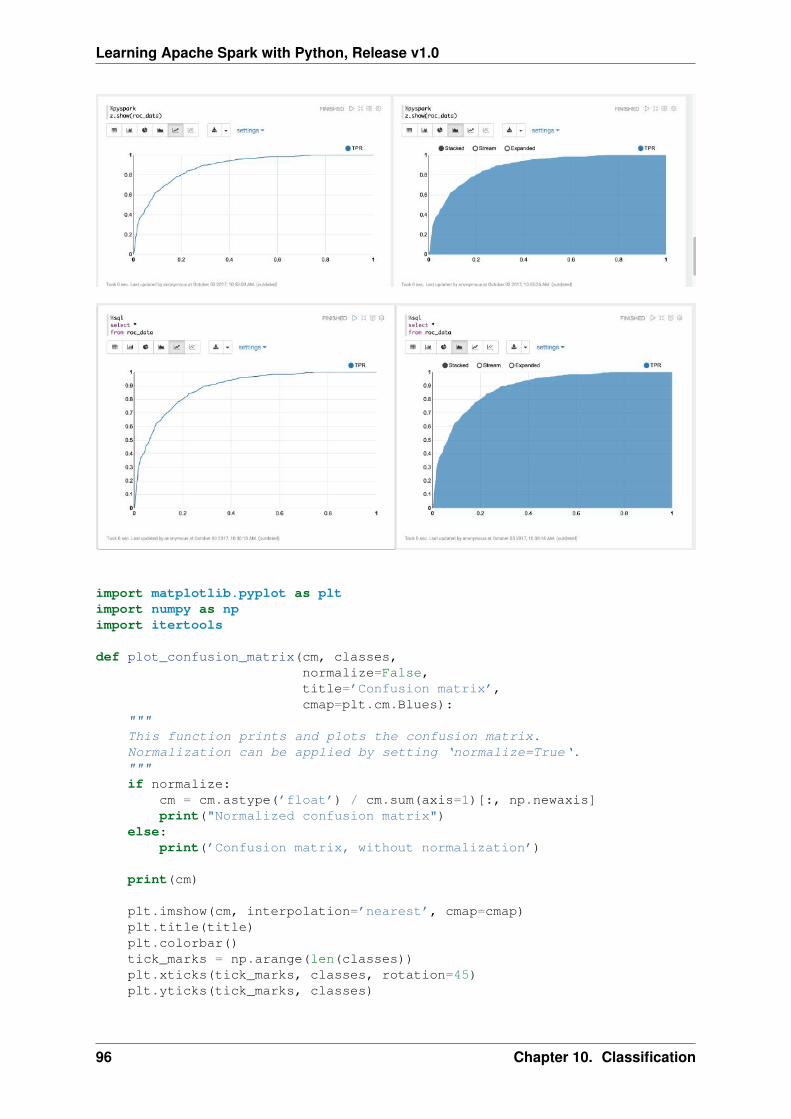
Learning Apache Spark with Python, Release v1.0
import matplotlib.pyplot as pltimport numpy as npimport itertools
def plot_confusion_matrix(cm, classes,normalize=False,title=’Confusion matrix’,cmap=plt.cm.Blues):
"""This function prints and plots the confusion matrix.Normalization can be applied by setting ‘normalize=True‘."""if normalize:
cm = cm.astype(’float’) / cm.sum(axis=1)[:, np.newaxis]print("Normalized confusion matrix")
else:print(’Confusion matrix, without normalization’)
print(cm)
plt.imshow(cm, interpolation=’nearest’, cmap=cmap)plt.title(title)plt.colorbar()tick_marks = np.arange(len(classes))plt.xticks(tick_marks, classes, rotation=45)plt.yticks(tick_marks, classes)
96 Chapter 10. Classification
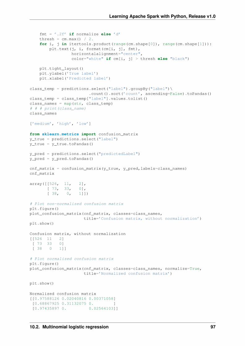
Learning Apache Spark with Python, Release v1.0
fmt = ’.2f’ if normalize else ’d’thresh = cm.max() / 2.for i, j in itertools.product(range(cm.shape[0]), range(cm.shape[1])):
plt.text(j, i, format(cm[i, j], fmt),horizontalalignment="center",color="white" if cm[i, j] > thresh else "black")
plt.tight_layout()plt.ylabel(’True label’)plt.xlabel(’Predicted label’)
class_temp = predictions.select("label").groupBy("label")\.count().sort(’count’, ascending=False).toPandas()
class_temp = class_temp["label"].values.tolist()class_names = map(str, class_temp)# # # print(class_name)class_names
[’medium’, ’high’, ’low’]
from sklearn.metrics import confusion_matrixy_true = predictions.select("label")y_true = y_true.toPandas()
y_pred = predictions.select("predictedLabel")y_pred = y_pred.toPandas()
cnf_matrix = confusion_matrix(y_true, y_pred,labels=class_names)cnf_matrix
array([[526, 11, 2],[ 73, 33, 0],[ 38, 0, 1]])
# Plot non-normalized confusion matrixplt.figure()plot_confusion_matrix(cnf_matrix, classes=class_names,
title=’Confusion matrix, without normalization’)plt.show()
Confusion matrix, without normalization[[526 11 2][ 73 33 0][ 38 0 1]]
# Plot normalized confusion matrixplt.figure()plot_confusion_matrix(cnf_matrix, classes=class_names, normalize=True,
title=’Normalized confusion matrix’)
plt.show()
Normalized confusion matrix[[0.97588126 0.02040816 0.00371058][0.68867925 0.31132075 0. ][0.97435897 0. 0.02564103]]
10.2. Multinomial logistic regression 97
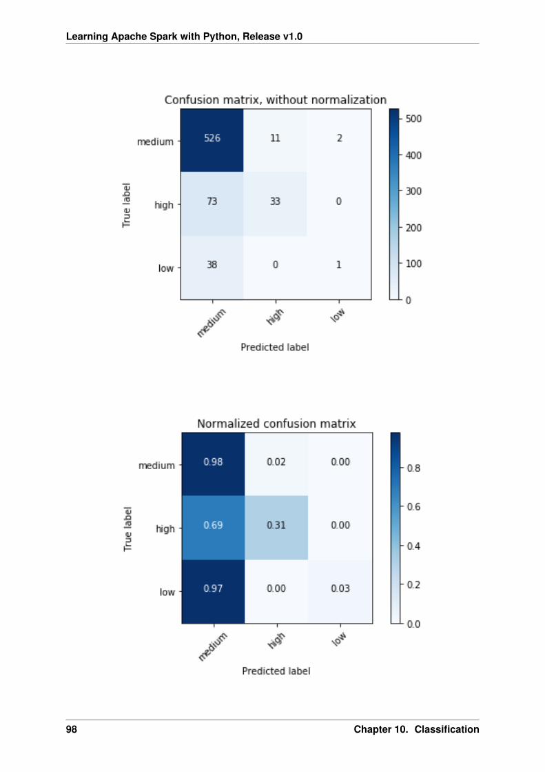
Learning Apache Spark with Python, Release v1.0
98 Chapter 10. Classification
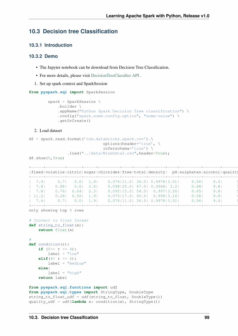
Learning Apache Spark with Python, Release v1.0
10.3 Decision tree Classification
10.3.1 Introduction
10.3.2 Demo
• The Jupyter notebook can be download from Decision Tree Classification.
• For more details, please visit DecisionTreeClassifier API .
1. Set up spark context and SparkSession
from pyspark.sql import SparkSession
spark = SparkSession \.builder \.appName("Python Spark Decision Tree classification") \.config("spark.some.config.option", "some-value") \.getOrCreate()
2. Load dataset
df = spark.read.format(’com.databricks.spark.csv’).\options(header=’true’, \inferschema=’true’) \
.load("../data/WineData2.csv",header=True);df.show(5,True)
+-----+--------+------+-----+---------+----+-----+-------+----+---------+-------+-------+|fixed|volatile|citric|sugar|chlorides|free|total|density| pH|sulphates|alcohol|quality|+-----+--------+------+-----+---------+----+-----+-------+----+---------+-------+-------+| 7.4| 0.7| 0.0| 1.9| 0.076|11.0| 34.0| 0.9978|3.51| 0.56| 9.4| 5|| 7.8| 0.88| 0.0| 2.6| 0.098|25.0| 67.0| 0.9968| 3.2| 0.68| 9.8| 5|| 7.8| 0.76| 0.04| 2.3| 0.092|15.0| 54.0| 0.997|3.26| 0.65| 9.8| 5|| 11.2| 0.28| 0.56| 1.9| 0.075|17.0| 60.0| 0.998|3.16| 0.58| 9.8| 6|| 7.4| 0.7| 0.0| 1.9| 0.076|11.0| 34.0| 0.9978|3.51| 0.56| 9.4| 5|+-----+--------+------+-----+---------+----+-----+-------+----+---------+-------+-------+only showing top 5 rows
# Convert to float formatdef string_to_float(x):
return float(x)
#def condition(r):
if (0<= r <= 4):label = "low"
elif(4< r <= 6):label = "medium"
else:label = "high"
return label
from pyspark.sql.functions import udffrom pyspark.sql.types import StringType, DoubleTypestring_to_float_udf = udf(string_to_float, DoubleType())quality_udf = udf(lambda x: condition(x), StringType())
10.3. Decision tree Classification 99
Learning Apache Spark with Python, Release v1.0
df = df.withColumn("quality", quality_udf("quality"))df.show(5,True)df.printSchema()
+-----+--------+------+-----+---------+----+-----+-------+----+---------+-------+-------+|fixed|volatile|citric|sugar|chlorides|free|total|density| pH|sulphates|alcohol|quality|+-----+--------+------+-----+---------+----+-----+-------+----+---------+-------+-------+| 7.4| 0.7| 0.0| 1.9| 0.076|11.0| 34.0| 0.9978|3.51| 0.56| 9.4| medium|| 7.8| 0.88| 0.0| 2.6| 0.098|25.0| 67.0| 0.9968| 3.2| 0.68| 9.8| medium|| 7.8| 0.76| 0.04| 2.3| 0.092|15.0| 54.0| 0.997|3.26| 0.65| 9.8| medium|| 11.2| 0.28| 0.56| 1.9| 0.075|17.0| 60.0| 0.998|3.16| 0.58| 9.8| medium|| 7.4| 0.7| 0.0| 1.9| 0.076|11.0| 34.0| 0.9978|3.51| 0.56| 9.4| medium|+-----+--------+------+-----+---------+----+-----+-------+----+---------+-------+-------+only showing top 5 rows
root|-- fixed: double (nullable = true)|-- volatile: double (nullable = true)|-- citric: double (nullable = true)|-- sugar: double (nullable = true)|-- chlorides: double (nullable = true)|-- free: double (nullable = true)|-- total: double (nullable = true)|-- density: double (nullable = true)|-- pH: double (nullable = true)|-- sulphates: double (nullable = true)|-- alcohol: double (nullable = true)|-- quality: string (nullable = true)
3. Convert the data to dense vector
Note: You are strongly encouraged to try my get_dummy function for dealing with the categoricaldata in complex dataset.
Supervised learning version:
def get_dummy(df,indexCol,categoricalCols,continuousCols,labelCol):
from pyspark.ml import Pipelinefrom pyspark.ml.feature import StringIndexer, OneHotEncoder, VectorAssemblerfrom pyspark.sql.functions import col
indexers = [ StringIndexer(inputCol=c, outputCol="{0}_indexed".format(c))for c in categoricalCols ]
# default setting: dropLast=Trueencoders = [ OneHotEncoder(inputCol=indexer.getOutputCol(),
outputCol="{0}_encoded".format(indexer.getOutputCol()))for indexer in indexers ]
assembler = VectorAssembler(inputCols=[encoder.getOutputCol() for encoder in encoders]+ continuousCols, outputCol="features")
pipeline = Pipeline(stages=indexers + encoders + [assembler])
model=pipeline.fit(df)data = model.transform(df)
100 Chapter 10. Classification
Learning Apache Spark with Python, Release v1.0
data = data.withColumn(’label’,col(labelCol))
return data.select(indexCol,’features’,’label’)
Unsupervised learning version:
def get_dummy(df,indexCol,categoricalCols,continuousCols):’’’Get dummy variables and concat with continuous variables for unsupervised learning.:param df: the dataframe:param categoricalCols: the name list of the categorical data:param continuousCols: the name list of the numerical data:return k: feature matrix
:author: Wenqiang Feng:email: [email protected]’’’
indexers = [ StringIndexer(inputCol=c, outputCol="{0}_indexed".format(c))for c in categoricalCols ]
# default setting: dropLast=Trueencoders = [ OneHotEncoder(inputCol=indexer.getOutputCol(),
outputCol="{0}_encoded".format(indexer.getOutputCol()))for indexer in indexers ]
assembler = VectorAssembler(inputCols=[encoder.getOutputCol() for encoder in encoders]+ continuousCols, outputCol="features")
pipeline = Pipeline(stages=indexers + encoders + [assembler])
model=pipeline.fit(df)data = model.transform(df)
return data.select(indexCol,’features’)
# !!!!caution: not from pyspark.mllib.linalg import Vectorsfrom pyspark.ml.linalg import Vectorsfrom pyspark.ml import Pipelinefrom pyspark.ml.feature import IndexToString,StringIndexer, VectorIndexerfrom pyspark.ml.tuning import CrossValidator, ParamGridBuilderfrom pyspark.ml.evaluation import MulticlassClassificationEvaluator
def transData(data):return data.rdd.map(lambda r: [Vectors.dense(r[:-1]),r[-1]]).toDF([’features’,’label’])
4. Transform the dataset to DataFrame
transformed = transData(df)transformed.show(5)
+--------------------+------+| features| label|+--------------------+------+|[7.4,0.7,0.0,1.9,...|medium||[7.8,0.88,0.0,2.6...|medium||[7.8,0.76,0.04,2....|medium|
10.3. Decision tree Classification 101
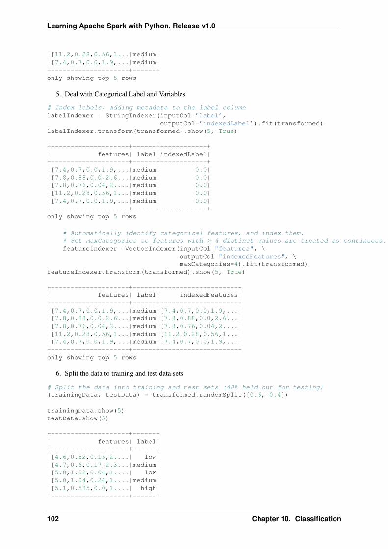
Learning Apache Spark with Python, Release v1.0
|[11.2,0.28,0.56,1...|medium||[7.4,0.7,0.0,1.9,...|medium|+--------------------+------+only showing top 5 rows
5. Deal with Categorical Label and Variables
# Index labels, adding metadata to the label columnlabelIndexer = StringIndexer(inputCol=’label’,
outputCol=’indexedLabel’).fit(transformed)labelIndexer.transform(transformed).show(5, True)
+--------------------+------+------------+| features| label|indexedLabel|+--------------------+------+------------+|[7.4,0.7,0.0,1.9,...|medium| 0.0||[7.8,0.88,0.0,2.6...|medium| 0.0||[7.8,0.76,0.04,2....|medium| 0.0||[11.2,0.28,0.56,1...|medium| 0.0||[7.4,0.7,0.0,1.9,...|medium| 0.0|+--------------------+------+------------+only showing top 5 rows
# Automatically identify categorical features, and index them.# Set maxCategories so features with > 4 distinct values are treated as continuous.featureIndexer =VectorIndexer(inputCol="features", \
outputCol="indexedFeatures", \maxCategories=4).fit(transformed)
featureIndexer.transform(transformed).show(5, True)
+--------------------+------+--------------------+| features| label| indexedFeatures|+--------------------+------+--------------------+|[7.4,0.7,0.0,1.9,...|medium|[7.4,0.7,0.0,1.9,...||[7.8,0.88,0.0,2.6...|medium|[7.8,0.88,0.0,2.6...||[7.8,0.76,0.04,2....|medium|[7.8,0.76,0.04,2....||[11.2,0.28,0.56,1...|medium|[11.2,0.28,0.56,1...||[7.4,0.7,0.0,1.9,...|medium|[7.4,0.7,0.0,1.9,...|+--------------------+------+--------------------+only showing top 5 rows
6. Split the data to training and test data sets
# Split the data into training and test sets (40% held out for testing)(trainingData, testData) = transformed.randomSplit([0.6, 0.4])
trainingData.show(5)testData.show(5)
+--------------------+------+| features| label|+--------------------+------+|[4.6,0.52,0.15,2....| low||[4.7,0.6,0.17,2.3...|medium||[5.0,1.02,0.04,1....| low||[5.0,1.04,0.24,1....|medium||[5.1,0.585,0.0,1....| high|+--------------------+------+
102 Chapter 10. Classification
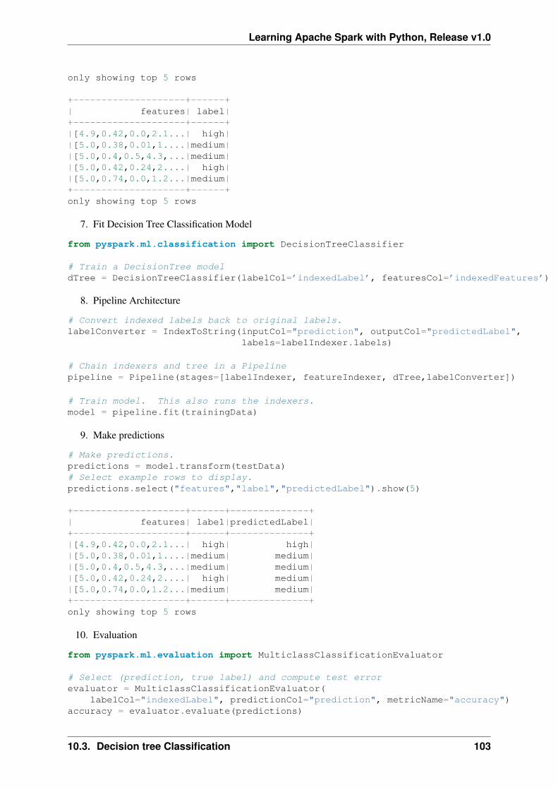
Learning Apache Spark with Python, Release v1.0
only showing top 5 rows
+--------------------+------+| features| label|+--------------------+------+|[4.9,0.42,0.0,2.1...| high||[5.0,0.38,0.01,1....|medium||[5.0,0.4,0.5,4.3,...|medium||[5.0,0.42,0.24,2....| high||[5.0,0.74,0.0,1.2...|medium|+--------------------+------+only showing top 5 rows
7. Fit Decision Tree Classification Model
from pyspark.ml.classification import DecisionTreeClassifier
# Train a DecisionTree modeldTree = DecisionTreeClassifier(labelCol=’indexedLabel’, featuresCol=’indexedFeatures’)
8. Pipeline Architecture
# Convert indexed labels back to original labels.labelConverter = IndexToString(inputCol="prediction", outputCol="predictedLabel",
labels=labelIndexer.labels)
# Chain indexers and tree in a Pipelinepipeline = Pipeline(stages=[labelIndexer, featureIndexer, dTree,labelConverter])
# Train model. This also runs the indexers.model = pipeline.fit(trainingData)
9. Make predictions
# Make predictions.predictions = model.transform(testData)# Select example rows to display.predictions.select("features","label","predictedLabel").show(5)
+--------------------+------+--------------+| features| label|predictedLabel|+--------------------+------+--------------+|[4.9,0.42,0.0,2.1...| high| high||[5.0,0.38,0.01,1....|medium| medium||[5.0,0.4,0.5,4.3,...|medium| medium||[5.0,0.42,0.24,2....| high| medium||[5.0,0.74,0.0,1.2...|medium| medium|+--------------------+------+--------------+only showing top 5 rows
10. Evaluation
from pyspark.ml.evaluation import MulticlassClassificationEvaluator
# Select (prediction, true label) and compute test errorevaluator = MulticlassClassificationEvaluator(
labelCol="indexedLabel", predictionCol="prediction", metricName="accuracy")accuracy = evaluator.evaluate(predictions)
10.3. Decision tree Classification 103
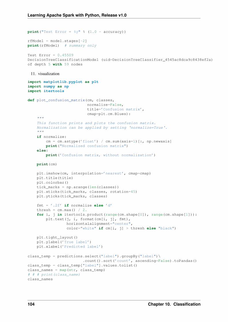
Learning Apache Spark with Python, Release v1.0
print("Test Error = %g" % (1.0 - accuracy))
rfModel = model.stages[-2]print(rfModel) # summary only
Test Error = 0.45509DecisionTreeClassificationModel (uid=DecisionTreeClassifier_4545ac8dca9c8438ef2a)of depth 5 with 59 nodes
11. visualization
import matplotlib.pyplot as pltimport numpy as npimport itertools
def plot_confusion_matrix(cm, classes,normalize=False,title=’Confusion matrix’,cmap=plt.cm.Blues):
"""This function prints and plots the confusion matrix.Normalization can be applied by setting ‘normalize=True‘."""if normalize:
cm = cm.astype(’float’) / cm.sum(axis=1)[:, np.newaxis]print("Normalized confusion matrix")
else:print(’Confusion matrix, without normalization’)
print(cm)
plt.imshow(cm, interpolation=’nearest’, cmap=cmap)plt.title(title)plt.colorbar()tick_marks = np.arange(len(classes))plt.xticks(tick_marks, classes, rotation=45)plt.yticks(tick_marks, classes)
fmt = ’.2f’ if normalize else ’d’thresh = cm.max() / 2.for i, j in itertools.product(range(cm.shape[0]), range(cm.shape[1])):
plt.text(j, i, format(cm[i, j], fmt),horizontalalignment="center",color="white" if cm[i, j] > thresh else "black")
plt.tight_layout()plt.ylabel(’True label’)plt.xlabel(’Predicted label’)
class_temp = predictions.select("label").groupBy("label")\.count().sort(’count’, ascending=False).toPandas()
class_temp = class_temp["label"].values.tolist()class_names = map(str, class_temp)# # # print(class_name)class_names
104 Chapter 10. Classification
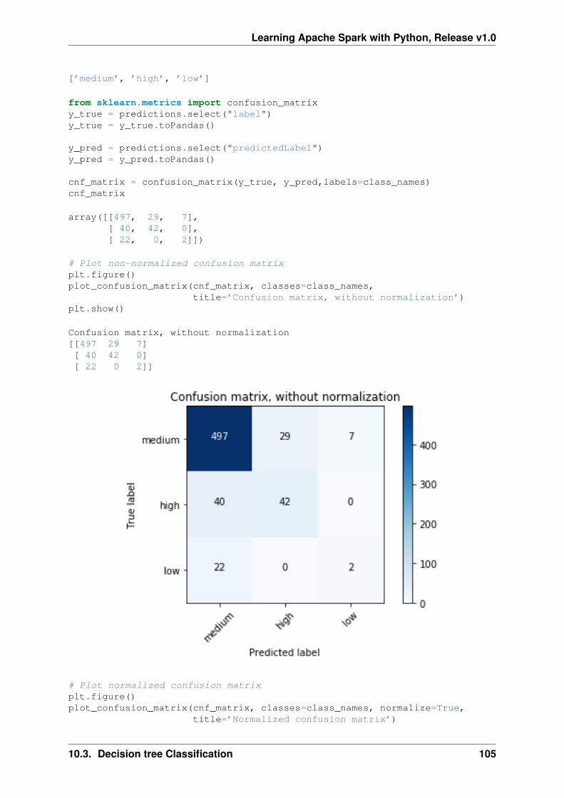
Learning Apache Spark with Python, Release v1.0
[’medium’, ’high’, ’low’]
from sklearn.metrics import confusion_matrixy_true = predictions.select("label")y_true = y_true.toPandas()
y_pred = predictions.select("predictedLabel")y_pred = y_pred.toPandas()
cnf_matrix = confusion_matrix(y_true, y_pred,labels=class_names)cnf_matrix
array([[497, 29, 7],[ 40, 42, 0],[ 22, 0, 2]])
# Plot non-normalized confusion matrixplt.figure()plot_confusion_matrix(cnf_matrix, classes=class_names,
title=’Confusion matrix, without normalization’)plt.show()
Confusion matrix, without normalization[[497 29 7][ 40 42 0][ 22 0 2]]
# Plot normalized confusion matrixplt.figure()plot_confusion_matrix(cnf_matrix, classes=class_names, normalize=True,
title=’Normalized confusion matrix’)
10.3. Decision tree Classification 105
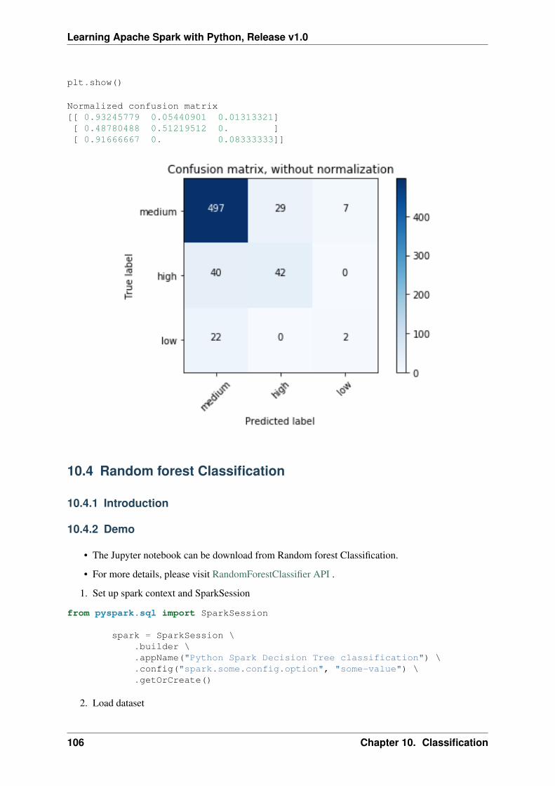
Learning Apache Spark with Python, Release v1.0
plt.show()
Normalized confusion matrix[[ 0.93245779 0.05440901 0.01313321][ 0.48780488 0.51219512 0. ][ 0.91666667 0. 0.08333333]]
10.4 Random forest Classification
10.4.1 Introduction
10.4.2 Demo
• The Jupyter notebook can be download from Random forest Classification.
• For more details, please visit RandomForestClassifier API .
1. Set up spark context and SparkSession
from pyspark.sql import SparkSession
spark = SparkSession \.builder \.appName("Python Spark Decision Tree classification") \.config("spark.some.config.option", "some-value") \.getOrCreate()
2. Load dataset
106 Chapter 10. Classification
Learning Apache Spark with Python, Release v1.0
df = spark.read.format(’com.databricks.spark.csv’).\options(header=’true’, \inferschema=’true’) \
.load("../data/WineData2.csv",header=True);df.show(5,True)
+-----+--------+------+-----+---------+----+-----+-------+----+---------+-------+-------+|fixed|volatile|citric|sugar|chlorides|free|total|density| pH|sulphates|alcohol|quality|+-----+--------+------+-----+---------+----+-----+-------+----+---------+-------+-------+| 7.4| 0.7| 0.0| 1.9| 0.076|11.0| 34.0| 0.9978|3.51| 0.56| 9.4| 5|| 7.8| 0.88| 0.0| 2.6| 0.098|25.0| 67.0| 0.9968| 3.2| 0.68| 9.8| 5|| 7.8| 0.76| 0.04| 2.3| 0.092|15.0| 54.0| 0.997|3.26| 0.65| 9.8| 5|| 11.2| 0.28| 0.56| 1.9| 0.075|17.0| 60.0| 0.998|3.16| 0.58| 9.8| 6|| 7.4| 0.7| 0.0| 1.9| 0.076|11.0| 34.0| 0.9978|3.51| 0.56| 9.4| 5|+-----+--------+------+-----+---------+----+-----+-------+----+---------+-------+-------+only showing top 5 rows
# Convert to float formatdef string_to_float(x):
return float(x)
#def condition(r):
if (0<= r <= 4):label = "low"
elif(4< r <= 6):label = "medium"
else:label = "high"
return label
from pyspark.sql.functions import udffrom pyspark.sql.types import StringType, DoubleTypestring_to_float_udf = udf(string_to_float, DoubleType())quality_udf = udf(lambda x: condition(x), StringType())
df = df.withColumn("quality", quality_udf("quality"))df.show(5,True)df.printSchema()
+-----+--------+------+-----+---------+----+-----+-------+----+---------+-------+-------+|fixed|volatile|citric|sugar|chlorides|free|total|density| pH|sulphates|alcohol|quality|+-----+--------+------+-----+---------+----+-----+-------+----+---------+-------+-------+| 7.4| 0.7| 0.0| 1.9| 0.076|11.0| 34.0| 0.9978|3.51| 0.56| 9.4| medium|| 7.8| 0.88| 0.0| 2.6| 0.098|25.0| 67.0| 0.9968| 3.2| 0.68| 9.8| medium|| 7.8| 0.76| 0.04| 2.3| 0.092|15.0| 54.0| 0.997|3.26| 0.65| 9.8| medium|| 11.2| 0.28| 0.56| 1.9| 0.075|17.0| 60.0| 0.998|3.16| 0.58| 9.8| medium|| 7.4| 0.7| 0.0| 1.9| 0.076|11.0| 34.0| 0.9978|3.51| 0.56| 9.4| medium|+-----+--------+------+-----+---------+----+-----+-------+----+---------+-------+-------+only showing top 5 rows
root|-- fixed: double (nullable = true)|-- volatile: double (nullable = true)|-- citric: double (nullable = true)|-- sugar: double (nullable = true)|-- chlorides: double (nullable = true)|-- free: double (nullable = true)
10.4. Random forest Classification 107
Learning Apache Spark with Python, Release v1.0
|-- total: double (nullable = true)|-- density: double (nullable = true)|-- pH: double (nullable = true)|-- sulphates: double (nullable = true)|-- alcohol: double (nullable = true)|-- quality: string (nullable = true)
3. Convert the data to dense vector
Note: You are strongly encouraged to try my get_dummy function for dealing with the categoricaldata in complex dataset.
Supervised learning version:
def get_dummy(df,indexCol,categoricalCols,continuousCols,labelCol):
from pyspark.ml import Pipelinefrom pyspark.ml.feature import StringIndexer, OneHotEncoder, VectorAssemblerfrom pyspark.sql.functions import col
indexers = [ StringIndexer(inputCol=c, outputCol="{0}_indexed".format(c))for c in categoricalCols ]
# default setting: dropLast=Trueencoders = [ OneHotEncoder(inputCol=indexer.getOutputCol(),
outputCol="{0}_encoded".format(indexer.getOutputCol()))for indexer in indexers ]
assembler = VectorAssembler(inputCols=[encoder.getOutputCol() for encoder in encoders]+ continuousCols, outputCol="features")
pipeline = Pipeline(stages=indexers + encoders + [assembler])
model=pipeline.fit(df)data = model.transform(df)
data = data.withColumn(’label’,col(labelCol))
return data.select(indexCol,’features’,’label’)
Unsupervised learning version:
def get_dummy(df,indexCol,categoricalCols,continuousCols):’’’Get dummy variables and concat with continuous variables for unsupervised learning.:param df: the dataframe:param categoricalCols: the name list of the categorical data:param continuousCols: the name list of the numerical data:return k: feature matrix
:author: Wenqiang Feng:email: [email protected]’’’
indexers = [ StringIndexer(inputCol=c, outputCol="{0}_indexed".format(c))for c in categoricalCols ]
# default setting: dropLast=True
108 Chapter 10. Classification
Learning Apache Spark with Python, Release v1.0
encoders = [ OneHotEncoder(inputCol=indexer.getOutputCol(),outputCol="{0}_encoded".format(indexer.getOutputCol()))for indexer in indexers ]
assembler = VectorAssembler(inputCols=[encoder.getOutputCol() for encoder in encoders]+ continuousCols, outputCol="features")
pipeline = Pipeline(stages=indexers + encoders + [assembler])
model=pipeline.fit(df)data = model.transform(df)
return data.select(indexCol,’features’)
# !!!!caution: not from pyspark.mllib.linalg import Vectorsfrom pyspark.ml.linalg import Vectorsfrom pyspark.ml import Pipelinefrom pyspark.ml.feature import IndexToString,StringIndexer, VectorIndexerfrom pyspark.ml.tuning import CrossValidator, ParamGridBuilderfrom pyspark.ml.evaluation import MulticlassClassificationEvaluator
def transData(data):return data.rdd.map(lambda r: [Vectors.dense(r[:-1]),r[-1]]).toDF([’features’,’label’])
4. Transform the dataset to DataFrame
transformed = transData(df)transformed.show(5)
+--------------------+------+| features| label|+--------------------+------+|[7.4,0.7,0.0,1.9,...|medium||[7.8,0.88,0.0,2.6...|medium||[7.8,0.76,0.04,2....|medium||[11.2,0.28,0.56,1...|medium||[7.4,0.7,0.0,1.9,...|medium|+--------------------+------+only showing top 5 rows
5. Deal with Categorical Label and Variables
# Index labels, adding metadata to the label columnlabelIndexer = StringIndexer(inputCol=’label’,
outputCol=’indexedLabel’).fit(transformed)labelIndexer.transform(transformed).show(5, True)
+--------------------+------+------------+| features| label|indexedLabel|+--------------------+------+------------+|[7.4,0.7,0.0,1.9,...|medium| 0.0||[7.8,0.88,0.0,2.6...|medium| 0.0||[7.8,0.76,0.04,2....|medium| 0.0||[11.2,0.28,0.56,1...|medium| 0.0||[7.4,0.7,0.0,1.9,...|medium| 0.0|+--------------------+------+------------+only showing top 5 rows
10.4. Random forest Classification 109
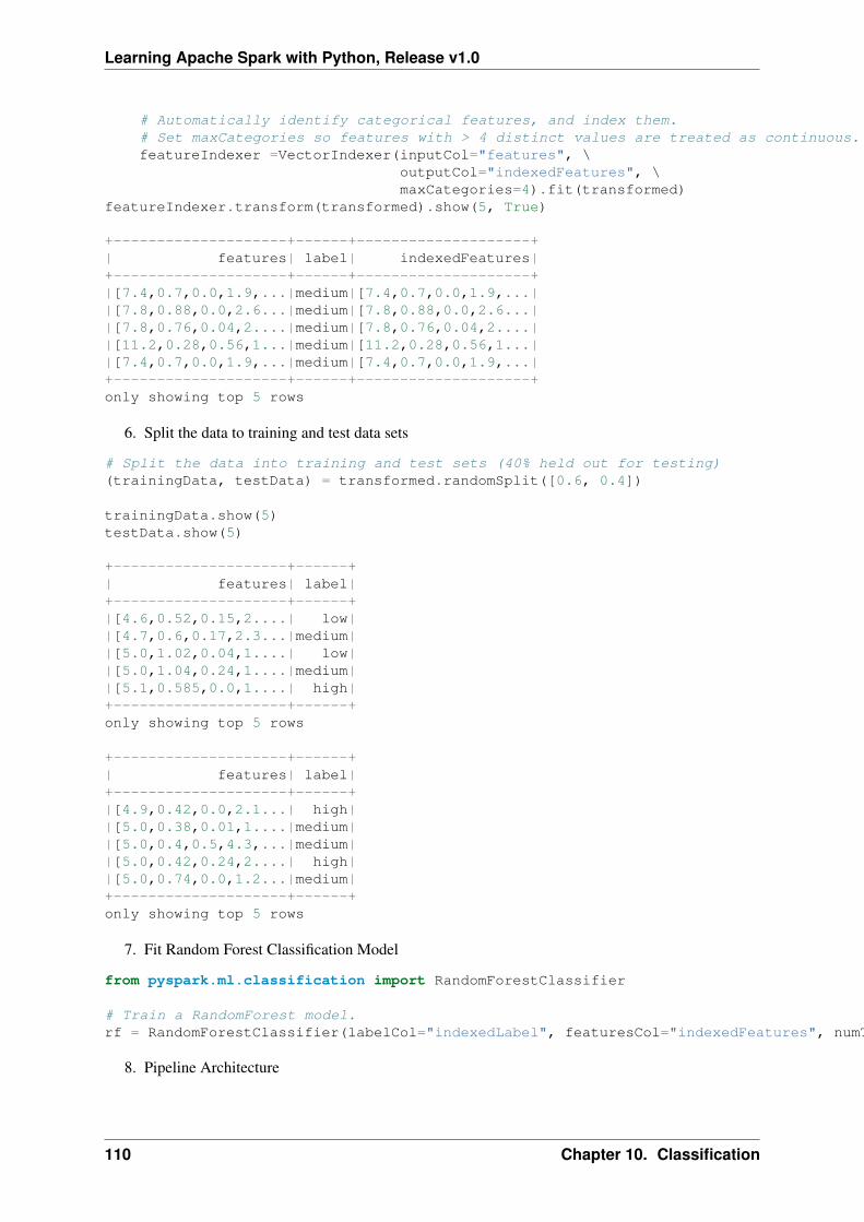
Learning Apache Spark with Python, Release v1.0
# Automatically identify categorical features, and index them.# Set maxCategories so features with > 4 distinct values are treated as continuous.featureIndexer =VectorIndexer(inputCol="features", \
outputCol="indexedFeatures", \maxCategories=4).fit(transformed)
featureIndexer.transform(transformed).show(5, True)
+--------------------+------+--------------------+| features| label| indexedFeatures|+--------------------+------+--------------------+|[7.4,0.7,0.0,1.9,...|medium|[7.4,0.7,0.0,1.9,...||[7.8,0.88,0.0,2.6...|medium|[7.8,0.88,0.0,2.6...||[7.8,0.76,0.04,2....|medium|[7.8,0.76,0.04,2....||[11.2,0.28,0.56,1...|medium|[11.2,0.28,0.56,1...||[7.4,0.7,0.0,1.9,...|medium|[7.4,0.7,0.0,1.9,...|+--------------------+------+--------------------+only showing top 5 rows
6. Split the data to training and test data sets
# Split the data into training and test sets (40% held out for testing)(trainingData, testData) = transformed.randomSplit([0.6, 0.4])
trainingData.show(5)testData.show(5)
+--------------------+------+| features| label|+--------------------+------+|[4.6,0.52,0.15,2....| low||[4.7,0.6,0.17,2.3...|medium||[5.0,1.02,0.04,1....| low||[5.0,1.04,0.24,1....|medium||[5.1,0.585,0.0,1....| high|+--------------------+------+only showing top 5 rows
+--------------------+------+| features| label|+--------------------+------+|[4.9,0.42,0.0,2.1...| high||[5.0,0.38,0.01,1....|medium||[5.0,0.4,0.5,4.3,...|medium||[5.0,0.42,0.24,2....| high||[5.0,0.74,0.0,1.2...|medium|+--------------------+------+only showing top 5 rows
7. Fit Random Forest Classification Model
from pyspark.ml.classification import RandomForestClassifier
# Train a RandomForest model.rf = RandomForestClassifier(labelCol="indexedLabel", featuresCol="indexedFeatures", numTrees=10)
8. Pipeline Architecture
110 Chapter 10. Classification
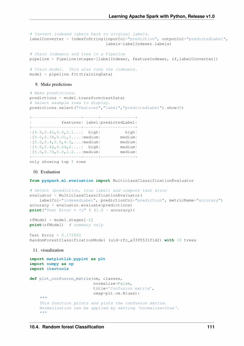
Learning Apache Spark with Python, Release v1.0
# Convert indexed labels back to original labels.labelConverter = IndexToString(inputCol="prediction", outputCol="predictedLabel",
labels=labelIndexer.labels)
# Chain indexers and tree in a Pipelinepipeline = Pipeline(stages=[labelIndexer, featureIndexer, rf,labelConverter])
# Train model. This also runs the indexers.model = pipeline.fit(trainingData)
9. Make predictions
# Make predictions.predictions = model.transform(testData)# Select example rows to display.predictions.select("features","label","predictedLabel").show(5)
+--------------------+------+--------------+| features| label|predictedLabel|+--------------------+------+--------------+|[4.9,0.42,0.0,2.1...| high| high||[5.0,0.38,0.01,1....|medium| medium||[5.0,0.4,0.5,4.3,...|medium| medium||[5.0,0.42,0.24,2....| high| medium||[5.0,0.74,0.0,1.2...|medium| medium|+--------------------+------+--------------+only showing top 5 rows
10. Evaluation
from pyspark.ml.evaluation import MulticlassClassificationEvaluator
# Select (prediction, true label) and compute test errorevaluator = MulticlassClassificationEvaluator(
labelCol="indexedLabel", predictionCol="prediction", metricName="accuracy")accuracy = evaluator.evaluate(predictions)print("Test Error = %g" % (1.0 - accuracy))
rfModel = model.stages[-2]print(rfModel) # summary only
Test Error = 0.173502RandomForestClassificationModel (uid=rfc_a3395531f1d2) with 10 trees
11. visualization
import matplotlib.pyplot as pltimport numpy as npimport itertools
def plot_confusion_matrix(cm, classes,normalize=False,title=’Confusion matrix’,cmap=plt.cm.Blues):
"""This function prints and plots the confusion matrix.Normalization can be applied by setting ‘normalize=True‘."""
10.4. Random forest Classification 111
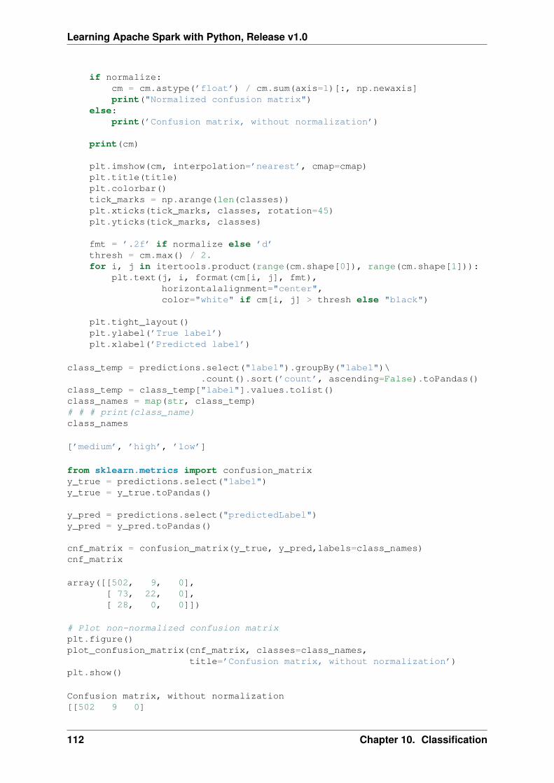
Learning Apache Spark with Python, Release v1.0
if normalize:cm = cm.astype(’float’) / cm.sum(axis=1)[:, np.newaxis]print("Normalized confusion matrix")
else:print(’Confusion matrix, without normalization’)
print(cm)
plt.imshow(cm, interpolation=’nearest’, cmap=cmap)plt.title(title)plt.colorbar()tick_marks = np.arange(len(classes))plt.xticks(tick_marks, classes, rotation=45)plt.yticks(tick_marks, classes)
fmt = ’.2f’ if normalize else ’d’thresh = cm.max() / 2.for i, j in itertools.product(range(cm.shape[0]), range(cm.shape[1])):
plt.text(j, i, format(cm[i, j], fmt),horizontalalignment="center",color="white" if cm[i, j] > thresh else "black")
plt.tight_layout()plt.ylabel(’True label’)plt.xlabel(’Predicted label’)
class_temp = predictions.select("label").groupBy("label")\.count().sort(’count’, ascending=False).toPandas()
class_temp = class_temp["label"].values.tolist()class_names = map(str, class_temp)# # # print(class_name)class_names
[’medium’, ’high’, ’low’]
from sklearn.metrics import confusion_matrixy_true = predictions.select("label")y_true = y_true.toPandas()
y_pred = predictions.select("predictedLabel")y_pred = y_pred.toPandas()
cnf_matrix = confusion_matrix(y_true, y_pred,labels=class_names)cnf_matrix
array([[502, 9, 0],[ 73, 22, 0],[ 28, 0, 0]])
# Plot non-normalized confusion matrixplt.figure()plot_confusion_matrix(cnf_matrix, classes=class_names,
title=’Confusion matrix, without normalization’)plt.show()
Confusion matrix, without normalization[[502 9 0]
112 Chapter 10. Classification
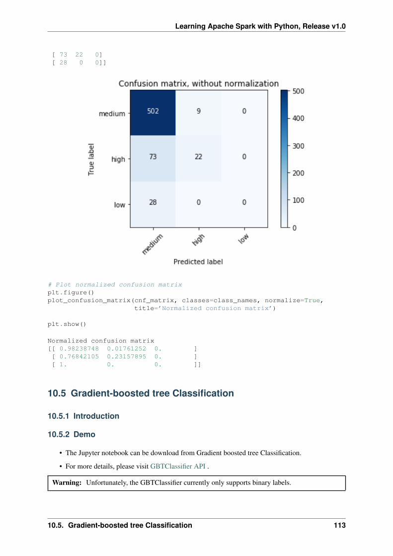
Learning Apache Spark with Python, Release v1.0
[ 73 22 0][ 28 0 0]]
# Plot normalized confusion matrixplt.figure()plot_confusion_matrix(cnf_matrix, classes=class_names, normalize=True,
title=’Normalized confusion matrix’)
plt.show()
Normalized confusion matrix[[ 0.98238748 0.01761252 0. ][ 0.76842105 0.23157895 0. ][ 1. 0. 0. ]]
10.5 Gradient-boosted tree Classification
10.5.1 Introduction
10.5.2 Demo
• The Jupyter notebook can be download from Gradient boosted tree Classification.
• For more details, please visit GBTClassifier API .
Warning: Unfortunately, the GBTClassifier currently only supports binary labels.
10.5. Gradient-boosted tree Classification 113
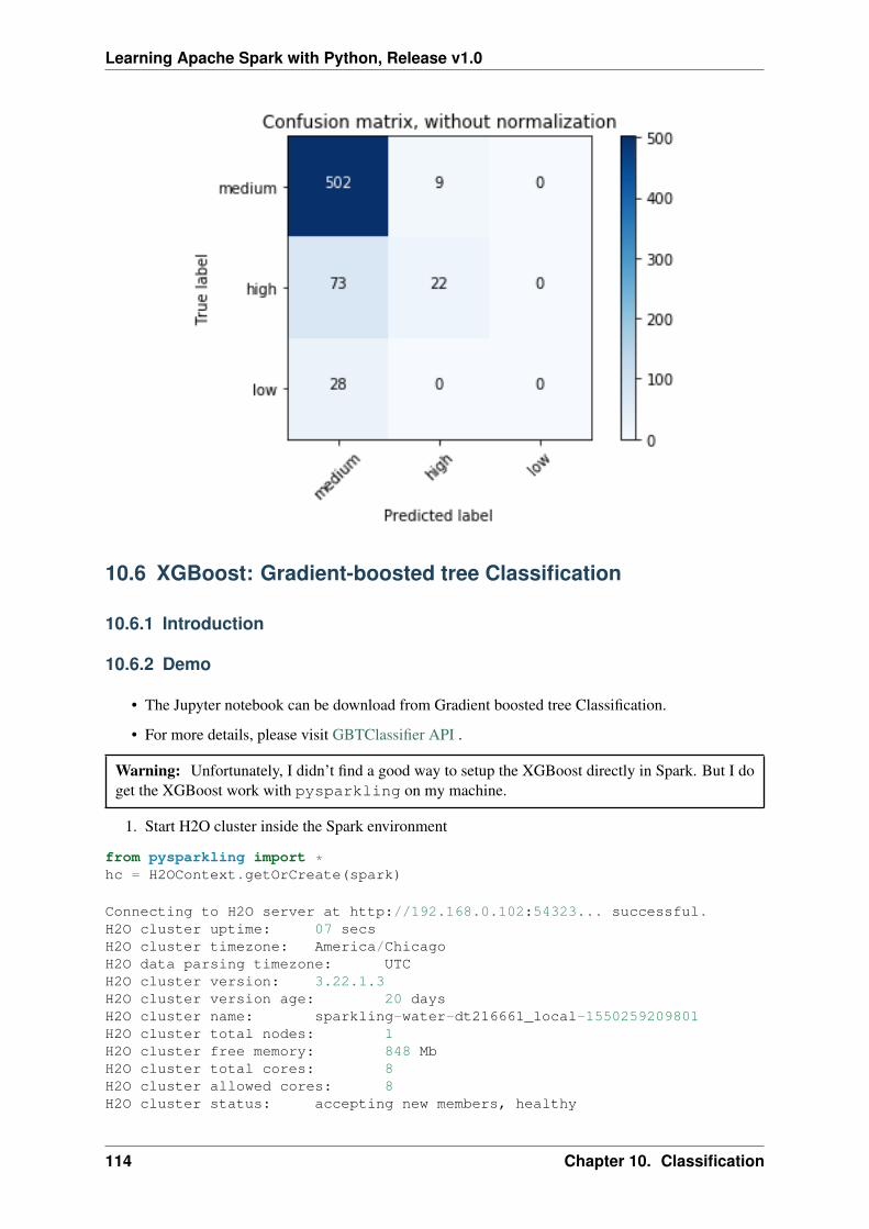
Learning Apache Spark with Python, Release v1.0
10.6 XGBoost: Gradient-boosted tree Classification
10.6.1 Introduction
10.6.2 Demo
• The Jupyter notebook can be download from Gradient boosted tree Classification.
• For more details, please visit GBTClassifier API .
Warning: Unfortunately, I didn’t find a good way to setup the XGBoost directly in Spark. But I doget the XGBoost work with pysparkling on my machine.
1. Start H2O cluster inside the Spark environment
from pysparkling import *hc = H2OContext.getOrCreate(spark)
Connecting to H2O server at http://192.168.0.102:54323... successful.H2O cluster uptime: 07 secsH2O cluster timezone: America/ChicagoH2O data parsing timezone: UTCH2O cluster version: 3.22.1.3H2O cluster version age: 20 daysH2O cluster name: sparkling-water-dt216661_local-1550259209801H2O cluster total nodes: 1H2O cluster free memory: 848 MbH2O cluster total cores: 8H2O cluster allowed cores: 8H2O cluster status: accepting new members, healthy
114 Chapter 10. Classification
Learning Apache Spark with Python, Release v1.0
H2O connection url: http://192.168.0.102:54323H2O connection proxy: NoneH2O internal security: FalseH2O API Extensions: XGBoost, Algos, AutoML, Core V3, Core V4Python version: 3.7.1 final
Sparkling Water Context:
* H2O name: sparkling-water-dt216661_local-1550259209801
* cluster size: 1
* list of used nodes:(executorId, host, port)------------------------(driver,192.168.0.102,54323)------------------------
Open H2O Flow in browser: http://192.168.0.102:54323 (CMD + click in Mac OSX)
2. Parse the data using H2O and convert them to Spark Frame
import h2oframe = h2o.import_file("https://raw.githubusercontent.com/h2oai/sparkling-water/master/examples/smalldata/prostate/prostate.csv")spark_frame = hc.as_spark_frame(frame)
spark_frame.show(4)
+---+-------+---+----+-----+-----+----+----+-------+| ID|CAPSULE|AGE|RACE|DPROS|DCAPS| PSA| VOL|GLEASON|+---+-------+---+----+-----+-----+----+----+-------+| 1| 0| 65| 1| 2| 1| 1.4| 0.0| 6|| 2| 0| 72| 1| 3| 2| 6.7| 0.0| 7|| 3| 0| 70| 1| 1| 2| 4.9| 0.0| 6|| 4| 0| 76| 2| 2| 1|51.2|20.0| 7|+---+-------+---+----+-----+-----+----+----+-------+only showing top 4 rows
3. Train the model
from pysparkling.ml import H2OXGBoostestimator = H2OXGBoost(predictionCol="AGE")model = estimator.fit(spark_frame)
4. Run Predictions
predictions = model.transform(spark_frame)predictions.show(4)
+---+-------+---+----+-----+-----+----+----+-------+-------------------+| ID|CAPSULE|AGE|RACE|DPROS|DCAPS| PSA| VOL|GLEASON| prediction_output|+---+-------+---+----+-----+-----+----+----+-------+-------------------+| 1| 0| 65| 1| 2| 1| 1.4| 0.0| 6|[64.85852813720703]|| 2| 0| 72| 1| 3| 2| 6.7| 0.0| 7| [72.0611801147461]|| 3| 0| 70| 1| 1| 2| 4.9| 0.0| 6|[70.26496887207031]|| 4| 0| 76| 2| 2| 1|51.2|20.0| 7|[75.26521301269531]|+---+-------+---+----+-----+-----+----+----+-------+-------------------+only showing top 4 rows
10.6. XGBoost: Gradient-boosted tree Classification 115
Learning Apache Spark with Python, Release v1.0
10.7 Naive Bayes Classification
10.7.1 Introduction
10.7.2 Demo
• The Jupyter notebook can be download from Naive Bayes Classification.
• For more details, please visit NaiveBayes API .
1. Set up spark context and SparkSession
from pyspark.sql import SparkSession
spark = SparkSession \.builder \.appName("Python Spark Naive Bayes classification") \.config("spark.some.config.option", "some-value") \.getOrCreate()
2. Load dataset
df = spark.read.format(’com.databricks.spark.csv’) \.options(header=’true’, inferschema=’true’) \.load("./data/WineData2.csv",header=True);
df.show(5)
+-----+--------+------+-----+---------+----+-----+-------+----+---------+-------+-------+|fixed|volatile|citric|sugar|chlorides|free|total|density| pH|sulphates|alcohol|quality|+-----+--------+------+-----+---------+----+-----+-------+----+---------+-------+-------+| 7.4| 0.7| 0.0| 1.9| 0.076|11.0| 34.0| 0.9978|3.51| 0.56| 9.4| 5|| 7.8| 0.88| 0.0| 2.6| 0.098|25.0| 67.0| 0.9968| 3.2| 0.68| 9.8| 5|| 7.8| 0.76| 0.04| 2.3| 0.092|15.0| 54.0| 0.997|3.26| 0.65| 9.8| 5|| 11.2| 0.28| 0.56| 1.9| 0.075|17.0| 60.0| 0.998|3.16| 0.58| 9.8| 6|| 7.4| 0.7| 0.0| 1.9| 0.076|11.0| 34.0| 0.9978|3.51| 0.56| 9.4| 5|+-----+--------+------+-----+---------+----+-----+-------+----+---------+-------+-------+only showing top 5 rows
df.printSchema()
root|-- fixed: double (nullable = true)|-- volatile: double (nullable = true)|-- citric: double (nullable = true)|-- sugar: double (nullable = true)|-- chlorides: double (nullable = true)|-- free: double (nullable = true)|-- total: double (nullable = true)|-- density: double (nullable = true)|-- pH: double (nullable = true)|-- sulphates: double (nullable = true)|-- alcohol: double (nullable = true)|-- quality: string (nullable = true)
# Convert to float formatdef string_to_float(x):
return float(x)
116 Chapter 10. Classification
Learning Apache Spark with Python, Release v1.0
#def condition(r):
if (0<= r <= 6):label = "low"
else:label = "high"
return label
from pyspark.sql.functions import udffrom pyspark.sql.types import StringType, DoubleTypestring_to_float_udf = udf(string_to_float, DoubleType())quality_udf = udf(lambda x: condition(x), StringType())
df = df.withColumn("quality", quality_udf("quality"))
df.show(5,True)
+-----+--------+------+-----+---------+----+-----+-------+----+---------+-------+-------+|fixed|volatile|citric|sugar|chlorides|free|total|density| pH|sulphates|alcohol|quality|+-----+--------+------+-----+---------+----+-----+-------+----+---------+-------+-------+| 7.4| 0.7| 0.0| 1.9| 0.076|11.0| 34.0| 0.9978|3.51| 0.56| 9.4| medium|| 7.8| 0.88| 0.0| 2.6| 0.098|25.0| 67.0| 0.9968| 3.2| 0.68| 9.8| medium|| 7.8| 0.76| 0.04| 2.3| 0.092|15.0| 54.0| 0.997|3.26| 0.65| 9.8| medium|| 11.2| 0.28| 0.56| 1.9| 0.075|17.0| 60.0| 0.998|3.16| 0.58| 9.8| medium|| 7.4| 0.7| 0.0| 1.9| 0.076|11.0| 34.0| 0.9978|3.51| 0.56| 9.4| medium|+-----+--------+------+-----+---------+----+-----+-------+----+---------+-------+-------+only showing top 5 rows
df.printSchema()
root|-- fixed: double (nullable = true)|-- volatile: double (nullable = true)|-- citric: double (nullable = true)|-- sugar: double (nullable = true)|-- chlorides: double (nullable = true)|-- free: double (nullable = true)|-- total: double (nullable = true)|-- density: double (nullable = true)|-- pH: double (nullable = true)|-- sulphates: double (nullable = true)|-- alcohol: double (nullable = true)|-- quality: string (nullable = true)
3. Deal with categorical data and Convert the data to dense vector
Note: You are strongly encouraged to try my get_dummy function for dealing with the categoricaldata in complex dataset.
Supervised learning version:
def get_dummy(df,indexCol,categoricalCols,continuousCols,labelCol):
from pyspark.ml import Pipelinefrom pyspark.ml.feature import StringIndexer, OneHotEncoder, VectorAssemblerfrom pyspark.sql.functions import col
10.7. Naive Bayes Classification 117
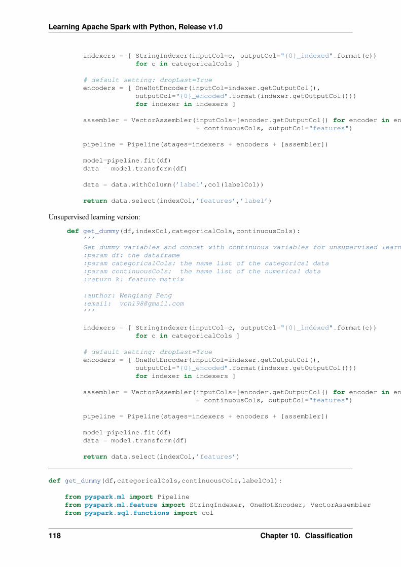
Learning Apache Spark with Python, Release v1.0
indexers = [ StringIndexer(inputCol=c, outputCol="{0}_indexed".format(c))for c in categoricalCols ]
# default setting: dropLast=Trueencoders = [ OneHotEncoder(inputCol=indexer.getOutputCol(),
outputCol="{0}_encoded".format(indexer.getOutputCol()))for indexer in indexers ]
assembler = VectorAssembler(inputCols=[encoder.getOutputCol() for encoder in encoders]+ continuousCols, outputCol="features")
pipeline = Pipeline(stages=indexers + encoders + [assembler])
model=pipeline.fit(df)data = model.transform(df)
data = data.withColumn(’label’,col(labelCol))
return data.select(indexCol,’features’,’label’)
Unsupervised learning version:
def get_dummy(df,indexCol,categoricalCols,continuousCols):’’’Get dummy variables and concat with continuous variables for unsupervised learning.:param df: the dataframe:param categoricalCols: the name list of the categorical data:param continuousCols: the name list of the numerical data:return k: feature matrix
:author: Wenqiang Feng:email: [email protected]’’’
indexers = [ StringIndexer(inputCol=c, outputCol="{0}_indexed".format(c))for c in categoricalCols ]
# default setting: dropLast=Trueencoders = [ OneHotEncoder(inputCol=indexer.getOutputCol(),
outputCol="{0}_encoded".format(indexer.getOutputCol()))for indexer in indexers ]
assembler = VectorAssembler(inputCols=[encoder.getOutputCol() for encoder in encoders]+ continuousCols, outputCol="features")
pipeline = Pipeline(stages=indexers + encoders + [assembler])
model=pipeline.fit(df)data = model.transform(df)
return data.select(indexCol,’features’)
def get_dummy(df,categoricalCols,continuousCols,labelCol):
from pyspark.ml import Pipelinefrom pyspark.ml.feature import StringIndexer, OneHotEncoder, VectorAssemblerfrom pyspark.sql.functions import col
118 Chapter 10. Classification
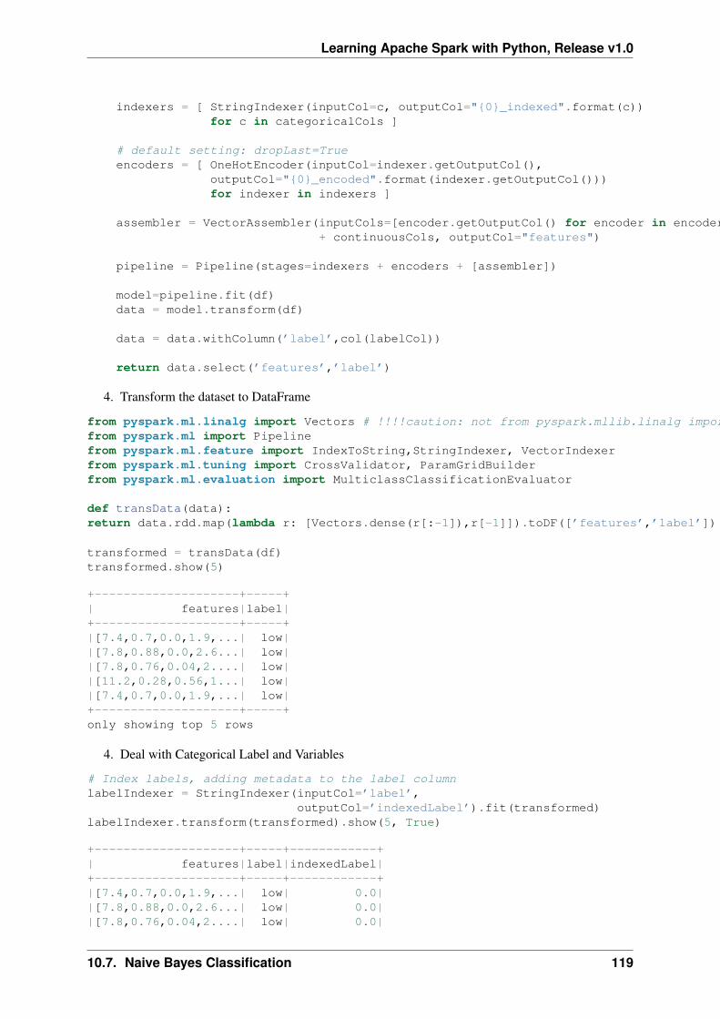
Learning Apache Spark with Python, Release v1.0
indexers = [ StringIndexer(inputCol=c, outputCol="{0}_indexed".format(c))for c in categoricalCols ]
# default setting: dropLast=Trueencoders = [ OneHotEncoder(inputCol=indexer.getOutputCol(),
outputCol="{0}_encoded".format(indexer.getOutputCol()))for indexer in indexers ]
assembler = VectorAssembler(inputCols=[encoder.getOutputCol() for encoder in encoders]+ continuousCols, outputCol="features")
pipeline = Pipeline(stages=indexers + encoders + [assembler])
model=pipeline.fit(df)data = model.transform(df)
data = data.withColumn(’label’,col(labelCol))
return data.select(’features’,’label’)
4. Transform the dataset to DataFrame
from pyspark.ml.linalg import Vectors # !!!!caution: not from pyspark.mllib.linalg import Vectorsfrom pyspark.ml import Pipelinefrom pyspark.ml.feature import IndexToString,StringIndexer, VectorIndexerfrom pyspark.ml.tuning import CrossValidator, ParamGridBuilderfrom pyspark.ml.evaluation import MulticlassClassificationEvaluator
def transData(data):return data.rdd.map(lambda r: [Vectors.dense(r[:-1]),r[-1]]).toDF([’features’,’label’])
transformed = transData(df)transformed.show(5)
+--------------------+-----+| features|label|+--------------------+-----+|[7.4,0.7,0.0,1.9,...| low||[7.8,0.88,0.0,2.6...| low||[7.8,0.76,0.04,2....| low||[11.2,0.28,0.56,1...| low||[7.4,0.7,0.0,1.9,...| low|+--------------------+-----+only showing top 5 rows
4. Deal with Categorical Label and Variables
# Index labels, adding metadata to the label columnlabelIndexer = StringIndexer(inputCol=’label’,
outputCol=’indexedLabel’).fit(transformed)labelIndexer.transform(transformed).show(5, True)
+--------------------+-----+------------+| features|label|indexedLabel|+--------------------+-----+------------+|[7.4,0.7,0.0,1.9,...| low| 0.0||[7.8,0.88,0.0,2.6...| low| 0.0||[7.8,0.76,0.04,2....| low| 0.0|
10.7. Naive Bayes Classification 119
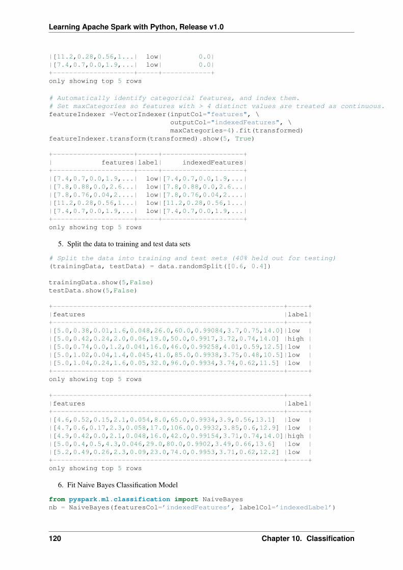
Learning Apache Spark with Python, Release v1.0
|[11.2,0.28,0.56,1...| low| 0.0||[7.4,0.7,0.0,1.9,...| low| 0.0|+--------------------+-----+------------+only showing top 5 rows
# Automatically identify categorical features, and index them.# Set maxCategories so features with > 4 distinct values are treated as continuous.featureIndexer =VectorIndexer(inputCol="features", \
outputCol="indexedFeatures", \maxCategories=4).fit(transformed)
featureIndexer.transform(transformed).show(5, True)
+--------------------+-----+--------------------+| features|label| indexedFeatures|+--------------------+-----+--------------------+|[7.4,0.7,0.0,1.9,...| low|[7.4,0.7,0.0,1.9,...||[7.8,0.88,0.0,2.6...| low|[7.8,0.88,0.0,2.6...||[7.8,0.76,0.04,2....| low|[7.8,0.76,0.04,2....||[11.2,0.28,0.56,1...| low|[11.2,0.28,0.56,1...||[7.4,0.7,0.0,1.9,...| low|[7.4,0.7,0.0,1.9,...|+--------------------+-----+--------------------+only showing top 5 rows
5. Split the data to training and test data sets
# Split the data into training and test sets (40% held out for testing)(trainingData, testData) = data.randomSplit([0.6, 0.4])
trainingData.show(5,False)testData.show(5,False)
+---------------------------------------------------------+-----+|features |label|+---------------------------------------------------------+-----+|[5.0,0.38,0.01,1.6,0.048,26.0,60.0,0.99084,3.7,0.75,14.0]|low ||[5.0,0.42,0.24,2.0,0.06,19.0,50.0,0.9917,3.72,0.74,14.0] |high ||[5.0,0.74,0.0,1.2,0.041,16.0,46.0,0.99258,4.01,0.59,12.5]|low ||[5.0,1.02,0.04,1.4,0.045,41.0,85.0,0.9938,3.75,0.48,10.5]|low ||[5.0,1.04,0.24,1.6,0.05,32.0,96.0,0.9934,3.74,0.62,11.5] |low |+---------------------------------------------------------+-----+only showing top 5 rows
+---------------------------------------------------------+-----+|features |label|+---------------------------------------------------------+-----+|[4.6,0.52,0.15,2.1,0.054,8.0,65.0,0.9934,3.9,0.56,13.1] |low ||[4.7,0.6,0.17,2.3,0.058,17.0,106.0,0.9932,3.85,0.6,12.9] |low ||[4.9,0.42,0.0,2.1,0.048,16.0,42.0,0.99154,3.71,0.74,14.0]|high ||[5.0,0.4,0.5,4.3,0.046,29.0,80.0,0.9902,3.49,0.66,13.6] |low ||[5.2,0.49,0.26,2.3,0.09,23.0,74.0,0.9953,3.71,0.62,12.2] |low |+---------------------------------------------------------+-----+only showing top 5 rows
6. Fit Naive Bayes Classification Model
from pyspark.ml.classification import NaiveBayesnb = NaiveBayes(featuresCol=’indexedFeatures’, labelCol=’indexedLabel’)
120 Chapter 10. Classification
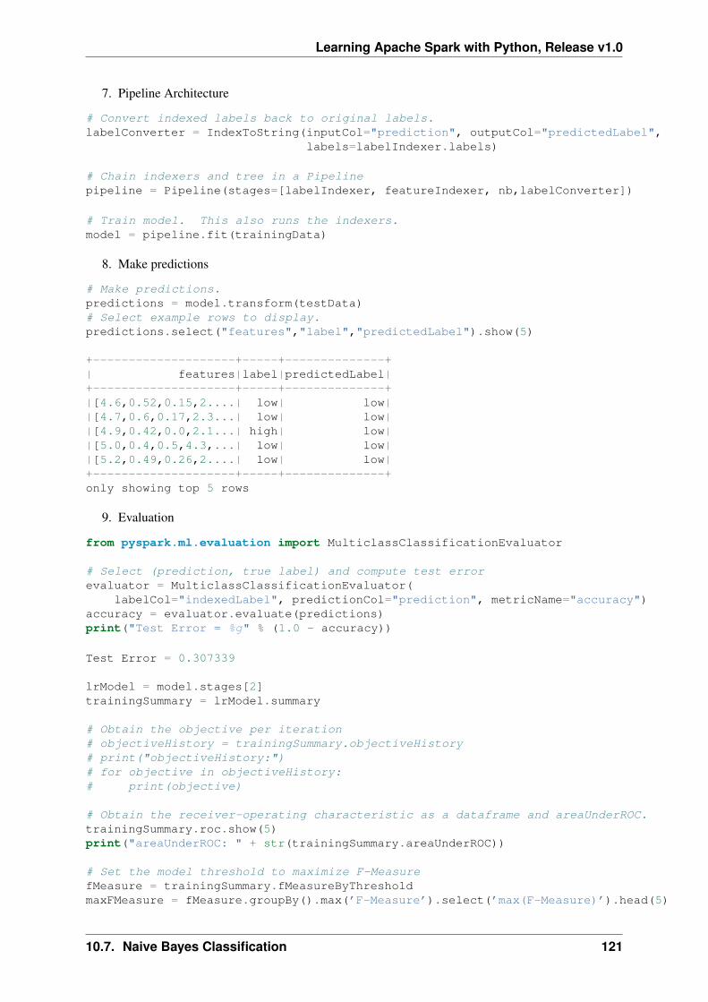
Learning Apache Spark with Python, Release v1.0
7. Pipeline Architecture
# Convert indexed labels back to original labels.labelConverter = IndexToString(inputCol="prediction", outputCol="predictedLabel",
labels=labelIndexer.labels)
# Chain indexers and tree in a Pipelinepipeline = Pipeline(stages=[labelIndexer, featureIndexer, nb,labelConverter])
# Train model. This also runs the indexers.model = pipeline.fit(trainingData)
8. Make predictions
# Make predictions.predictions = model.transform(testData)# Select example rows to display.predictions.select("features","label","predictedLabel").show(5)
+--------------------+-----+--------------+| features|label|predictedLabel|+--------------------+-----+--------------+|[4.6,0.52,0.15,2....| low| low||[4.7,0.6,0.17,2.3...| low| low||[4.9,0.42,0.0,2.1...| high| low||[5.0,0.4,0.5,4.3,...| low| low||[5.2,0.49,0.26,2....| low| low|+--------------------+-----+--------------+only showing top 5 rows
9. Evaluation
from pyspark.ml.evaluation import MulticlassClassificationEvaluator
# Select (prediction, true label) and compute test errorevaluator = MulticlassClassificationEvaluator(
labelCol="indexedLabel", predictionCol="prediction", metricName="accuracy")accuracy = evaluator.evaluate(predictions)print("Test Error = %g" % (1.0 - accuracy))
Test Error = 0.307339
lrModel = model.stages[2]trainingSummary = lrModel.summary
# Obtain the objective per iteration# objectiveHistory = trainingSummary.objectiveHistory# print("objectiveHistory:")# for objective in objectiveHistory:# print(objective)
# Obtain the receiver-operating characteristic as a dataframe and areaUnderROC.trainingSummary.roc.show(5)print("areaUnderROC: " + str(trainingSummary.areaUnderROC))
# Set the model threshold to maximize F-MeasurefMeasure = trainingSummary.fMeasureByThresholdmaxFMeasure = fMeasure.groupBy().max(’F-Measure’).select(’max(F-Measure)’).head(5)
10.7. Naive Bayes Classification 121
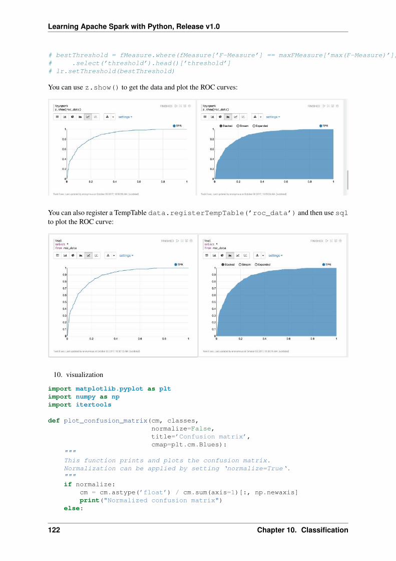
Learning Apache Spark with Python, Release v1.0
# bestThreshold = fMeasure.where(fMeasure[’F-Measure’] == maxFMeasure[’max(F-Measure)’]) \# .select(’threshold’).head()[’threshold’]# lr.setThreshold(bestThreshold)
You can use z.show() to get the data and plot the ROC curves:
You can also register a TempTable data.registerTempTable(’roc_data’) and then use sqlto plot the ROC curve:
10. visualization
import matplotlib.pyplot as pltimport numpy as npimport itertools
def plot_confusion_matrix(cm, classes,normalize=False,title=’Confusion matrix’,cmap=plt.cm.Blues):
"""This function prints and plots the confusion matrix.Normalization can be applied by setting ‘normalize=True‘."""if normalize:
cm = cm.astype(’float’) / cm.sum(axis=1)[:, np.newaxis]print("Normalized confusion matrix")
else:
122 Chapter 10. Classification
Learning Apache Spark with Python, Release v1.0
print(’Confusion matrix, without normalization’)
print(cm)
plt.imshow(cm, interpolation=’nearest’, cmap=cmap)plt.title(title)plt.colorbar()tick_marks = np.arange(len(classes))plt.xticks(tick_marks, classes, rotation=45)plt.yticks(tick_marks, classes)
fmt = ’.2f’ if normalize else ’d’thresh = cm.max() / 2.for i, j in itertools.product(range(cm.shape[0]), range(cm.shape[1])):
plt.text(j, i, format(cm[i, j], fmt),horizontalalignment="center",color="white" if cm[i, j] > thresh else "black")
plt.tight_layout()plt.ylabel(’True label’)plt.xlabel(’Predicted label’)
class_temp = predictions.select("label").groupBy("label")\.count().sort(’count’, ascending=False).toPandas()
class_temp = class_temp["label"].values.tolist()class_names = map(str, class_temp)# # # print(class_name)class_names
[’low’, ’high’]
from sklearn.metrics import confusion_matrixy_true = predictions.select("label")y_true = y_true.toPandas()
y_pred = predictions.select("predictedLabel")y_pred = y_pred.toPandas()
cnf_matrix = confusion_matrix(y_true, y_pred,labels=class_names)cnf_matrix
array([[392, 169],[ 32, 61]])
# Plot non-normalized confusion matrixplt.figure()plot_confusion_matrix(cnf_matrix, classes=class_names,
title=’Confusion matrix, without normalization’)plt.show()
Confusion matrix, without normalization[[392 169][ 32 61]]
# Plot normalized confusion matrixplt.figure()plot_confusion_matrix(cnf_matrix, classes=class_names, normalize=True,
10.7. Naive Bayes Classification 123
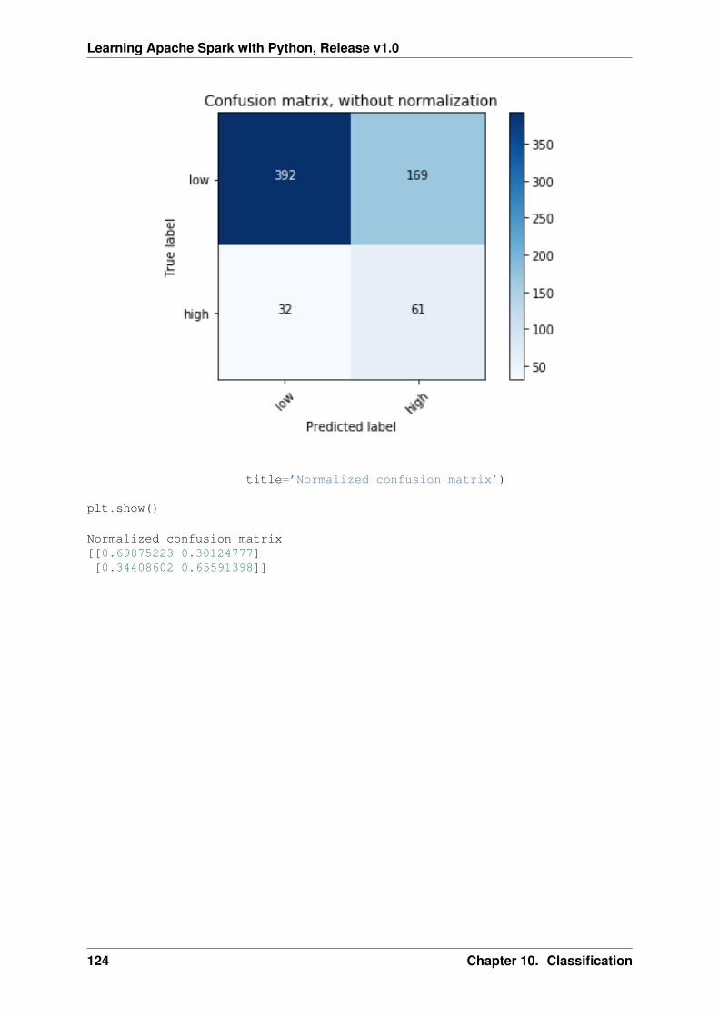
Learning Apache Spark with Python, Release v1.0
title=’Normalized confusion matrix’)
plt.show()
Normalized confusion matrix[[0.69875223 0.30124777][0.34408602 0.65591398]]
124 Chapter 10. Classification
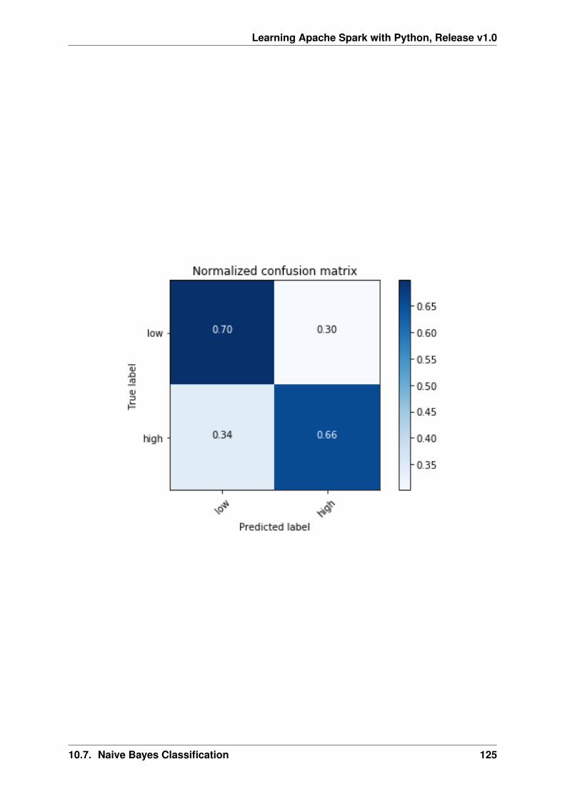
Learning Apache Spark with Python, Release v1.0
10.7. Naive Bayes Classification 125
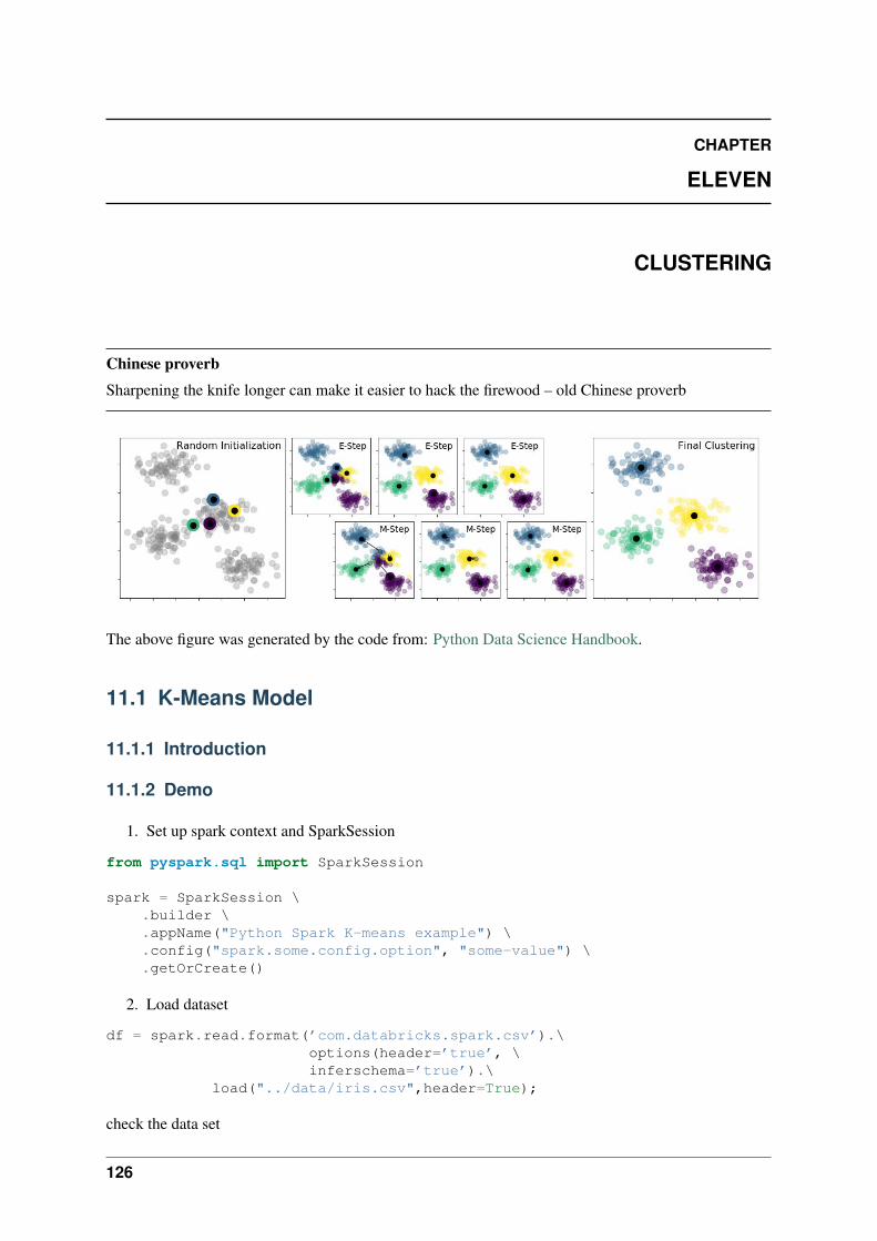
CHAPTER
ELEVEN
CLUSTERING
Chinese proverb
Sharpening the knife longer can make it easier to hack the firewood – old Chinese proverb
The above figure was generated by the code from: Python Data Science Handbook.
11.1 K-Means Model
11.1.1 Introduction
11.1.2 Demo
1. Set up spark context and SparkSession
from pyspark.sql import SparkSession
spark = SparkSession \.builder \.appName("Python Spark K-means example") \.config("spark.some.config.option", "some-value") \.getOrCreate()
2. Load dataset
df = spark.read.format(’com.databricks.spark.csv’).\options(header=’true’, \inferschema=’true’).\
load("../data/iris.csv",header=True);
check the data set
126
Learning Apache Spark with Python, Release v1.0
df.show(5,True)df.printSchema()
Then you will get
+------------+-----------+------------+-----------+-------+|sepal_length|sepal_width|petal_length|petal_width|species|+------------+-----------+------------+-----------+-------+| 5.1| 3.5| 1.4| 0.2| setosa|| 4.9| 3.0| 1.4| 0.2| setosa|| 4.7| 3.2| 1.3| 0.2| setosa|| 4.6| 3.1| 1.5| 0.2| setosa|| 5.0| 3.6| 1.4| 0.2| setosa|+------------+-----------+------------+-----------+-------+only showing top 5 rows
root|-- sepal_length: double (nullable = true)|-- sepal_width: double (nullable = true)|-- petal_length: double (nullable = true)|-- petal_width: double (nullable = true)|-- species: string (nullable = true)
You can also get the Statistical resutls from the data frame (Unfortunately, it only works for numerical).
df.describe().show()
Then you will get
+-------+------------------+-------------------+------------------+------------------+---------+|summary| sepal_length| sepal_width| petal_length| petal_width| species|+-------+------------------+-------------------+------------------+------------------+---------+| count| 150| 150| 150| 150| 150|| mean| 5.843333333333335| 3.0540000000000007|3.7586666666666693|1.1986666666666672| null|| stddev|0.8280661279778637|0.43359431136217375| 1.764420419952262|0.7631607417008414| null|| min| 4.3| 2.0| 1.0| 0.1| setosa|| max| 7.9| 4.4| 6.9| 2.5|virginica|+-------+------------------+-------------------+------------------+------------------+---------+
3. Convert the data to dense vector (features)
# convert the data to dense vectordef transData(data):
return data.rdd.map(lambda r: [Vectors.dense(r[:-1])]).toDF([’features’])
Note: You are strongly encouraged to try my get_dummy function for dealing with the categoricaldata in complex dataset.
Supervised learning version:
def get_dummy(df,indexCol,categoricalCols,continuousCols,labelCol):
from pyspark.ml import Pipelinefrom pyspark.ml.feature import StringIndexer, OneHotEncoder, VectorAssemblerfrom pyspark.sql.functions import col
indexers = [ StringIndexer(inputCol=c, outputCol="{0}_indexed".format(c))for c in categoricalCols ]
11.1. K-Means Model 127
Learning Apache Spark with Python, Release v1.0
# default setting: dropLast=Trueencoders = [ OneHotEncoder(inputCol=indexer.getOutputCol(),
outputCol="{0}_encoded".format(indexer.getOutputCol()))for indexer in indexers ]
assembler = VectorAssembler(inputCols=[encoder.getOutputCol() for encoder in encoders]+ continuousCols, outputCol="features")
pipeline = Pipeline(stages=indexers + encoders + [assembler])
model=pipeline.fit(df)data = model.transform(df)
data = data.withColumn(’label’,col(labelCol))
return data.select(indexCol,’features’,’label’)
Unsupervised learning version:
def get_dummy(df,indexCol,categoricalCols,continuousCols):’’’Get dummy variables and concat with continuous variables for unsupervised learning.:param df: the dataframe:param categoricalCols: the name list of the categorical data:param continuousCols: the name list of the numerical data:return k: feature matrix
:author: Wenqiang Feng:email: [email protected]’’’
indexers = [ StringIndexer(inputCol=c, outputCol="{0}_indexed".format(c))for c in categoricalCols ]
# default setting: dropLast=Trueencoders = [ OneHotEncoder(inputCol=indexer.getOutputCol(),
outputCol="{0}_encoded".format(indexer.getOutputCol()))for indexer in indexers ]
assembler = VectorAssembler(inputCols=[encoder.getOutputCol() for encoder in encoders]+ continuousCols, outputCol="features")
pipeline = Pipeline(stages=indexers + encoders + [assembler])
model=pipeline.fit(df)data = model.transform(df)
return data.select(indexCol,’features’)
4. Transform the dataset to DataFrame
transformed= transData(df)transformed.show(5, False)
+-----------------+|features |+-----------------+
128 Chapter 11. Clustering
Learning Apache Spark with Python, Release v1.0
|[5.1,3.5,1.4,0.2]||[4.9,3.0,1.4,0.2]||[4.7,3.2,1.3,0.2]||[4.6,3.1,1.5,0.2]||[5.0,3.6,1.4,0.2]|+-----------------+only showing top 5 rows
5. Deal With Categorical Variables
from pyspark.ml import Pipelinefrom pyspark.ml.regression import LinearRegressionfrom pyspark.ml.feature import VectorIndexerfrom pyspark.ml.evaluation import RegressionEvaluator
# Automatically identify categorical features, and index them.# We specify maxCategories so features with > 4 distinct values are treated as continuous.
featureIndexer = VectorIndexer(inputCol="features", \outputCol="indexedFeatures",\maxCategories=4).fit(transformed)
data = featureIndexer.transform(transformed)
Now you check your dataset with
data.show(5,True)
you will get
+-----------------+-----------------+| features| indexedFeatures|+-----------------+-----------------+|[5.1,3.5,1.4,0.2]|[5.1,3.5,1.4,0.2]||[4.9,3.0,1.4,0.2]|[4.9,3.0,1.4,0.2]||[4.7,3.2,1.3,0.2]|[4.7,3.2,1.3,0.2]||[4.6,3.1,1.5,0.2]|[4.6,3.1,1.5,0.2]||[5.0,3.6,1.4,0.2]|[5.0,3.6,1.4,0.2]|+-----------------+-----------------+only showing top 5 rows
6. Elbow method to determine the optimal number of clusters for k-means clustering
import numpy as npcost = np.zeros(20)for k in range(2,20):
kmeans = KMeans()\.setK(k)\.setSeed(1) \.setFeaturesCol("indexedFeatures")\.setPredictionCol("cluster")
model = kmeans.fit(data)cost[k] = model.computeCost(data) # requires Spark 2.0 or later
import numpy as npimport matplotlib.mlab as mlabimport matplotlib.pyplot as plt
11.1. K-Means Model 129
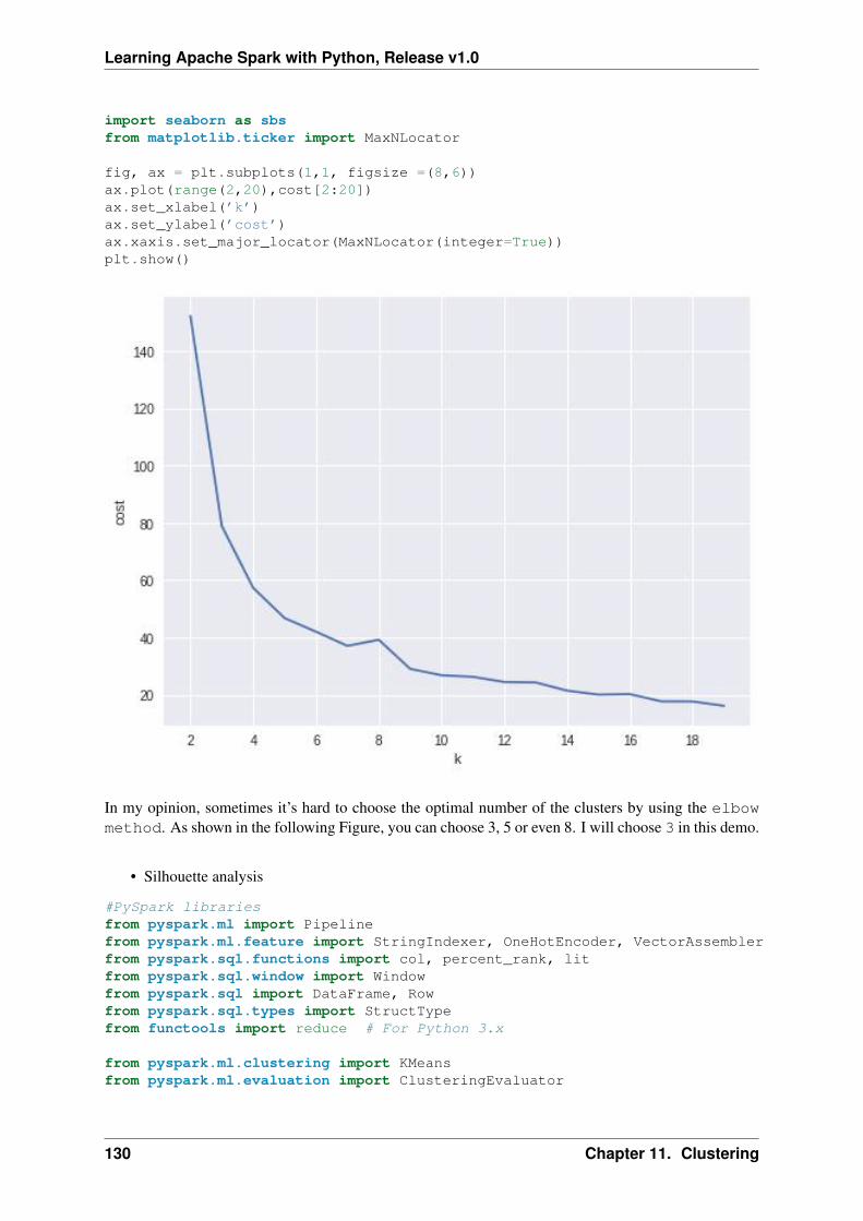
Learning Apache Spark with Python, Release v1.0
import seaborn as sbsfrom matplotlib.ticker import MaxNLocator
fig, ax = plt.subplots(1,1, figsize =(8,6))ax.plot(range(2,20),cost[2:20])ax.set_xlabel(’k’)ax.set_ylabel(’cost’)ax.xaxis.set_major_locator(MaxNLocator(integer=True))plt.show()
In my opinion, sometimes it’s hard to choose the optimal number of the clusters by using the elbowmethod. As shown in the following Figure, you can choose 3, 5 or even 8. I will choose 3 in this demo.
• Silhouette analysis
#PySpark librariesfrom pyspark.ml import Pipelinefrom pyspark.ml.feature import StringIndexer, OneHotEncoder, VectorAssemblerfrom pyspark.sql.functions import col, percent_rank, litfrom pyspark.sql.window import Windowfrom pyspark.sql import DataFrame, Rowfrom pyspark.sql.types import StructTypefrom functools import reduce # For Python 3.x
from pyspark.ml.clustering import KMeansfrom pyspark.ml.evaluation import ClusteringEvaluator
130 Chapter 11. Clustering
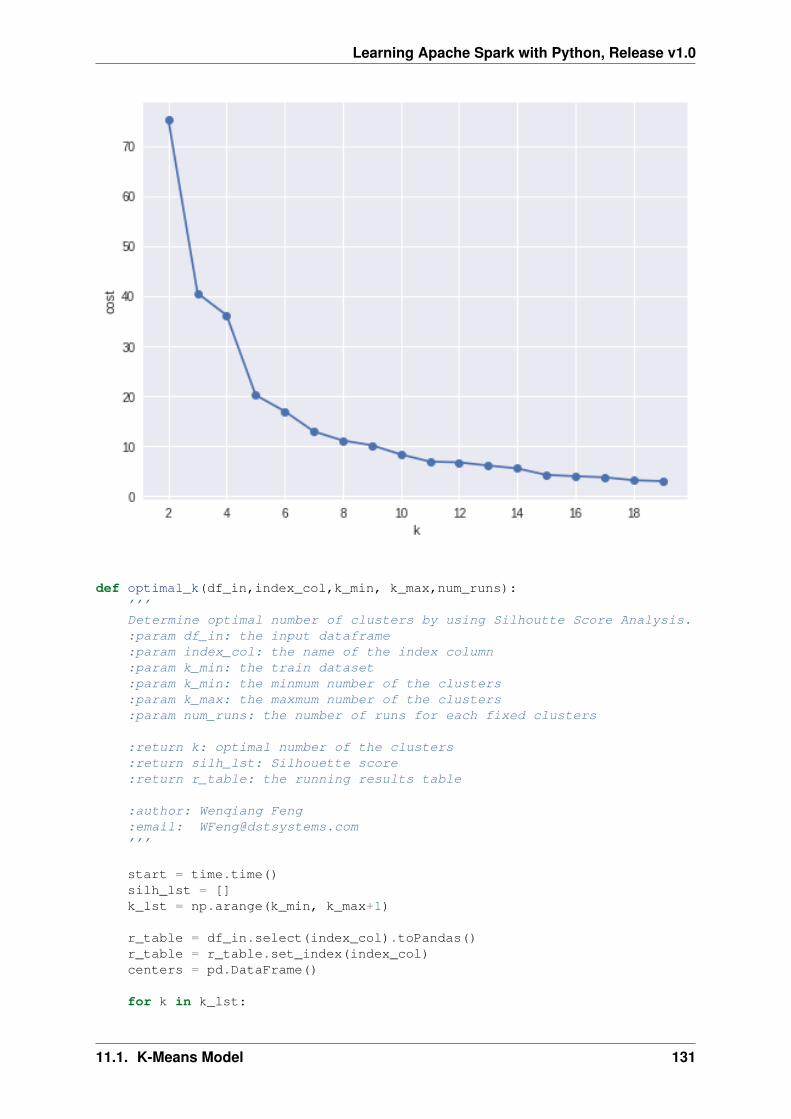
Learning Apache Spark with Python, Release v1.0
def optimal_k(df_in,index_col,k_min, k_max,num_runs):’’’Determine optimal number of clusters by using Silhoutte Score Analysis.:param df_in: the input dataframe:param index_col: the name of the index column:param k_min: the train dataset:param k_min: the minmum number of the clusters:param k_max: the maxmum number of the clusters:param num_runs: the number of runs for each fixed clusters
:return k: optimal number of the clusters:return silh_lst: Silhouette score:return r_table: the running results table
:author: Wenqiang Feng:email: [email protected]’’’
start = time.time()silh_lst = []k_lst = np.arange(k_min, k_max+1)
r_table = df_in.select(index_col).toPandas()r_table = r_table.set_index(index_col)centers = pd.DataFrame()
for k in k_lst:
11.1. K-Means Model 131
Learning Apache Spark with Python, Release v1.0
silh_val = []for run in np.arange(1, num_runs+1):
# Trains a k-means model.kmeans = KMeans()\
.setK(k)\
.setSeed(int(np.random.randint(100, size=1)))model = kmeans.fit(df_in)
# Make predictionspredictions = model.transform(df_in)r_table[’cluster_{k}_{run}’.format(k=k, run=run)]= predictions.select(’prediction’).toPandas()
# Evaluate clustering by computing Silhouette scoreevaluator = ClusteringEvaluator()silhouette = evaluator.evaluate(predictions)silh_val.append(silhouette)
silh_array=np.asanyarray(silh_val)silh_lst.append(silh_array.mean())
elapsed = time.time() - start
silhouette = pd.DataFrame(list(zip(k_lst,silh_lst)),columns = [’k’, ’silhouette’])
print(’+------------------------------------------------------------+’)print("| The finding optimal k phase took %8.0f s. |" %(elapsed))print(’+------------------------------------------------------------+’)
return k_lst[np.argmax(silh_lst, axis=0)], silhouette , r_table
k, silh_lst, r_table = optimal_k(scaledData,index_col,k_min, k_max,num_runs)
+------------------------------------------------------------+| The finding optimal k phase took 1783 s. |+------------------------------------------------------------+
spark.createDataFrame(silh_lst).show()
+---+------------------+| k| silhouette|+---+------------------+| 3|0.8045154385557953|| 4|0.6993528775512052|| 5|0.6689286654221447|| 6|0.6356184024841809|| 7|0.7174102265711756|| 8|0.6720861758298997|| 9| 0.601771359881241|| 10|0.6292447334578428|+---+------------------+
From the silhouette list, we can choose 3 as the optimal number of the clusters.
Warning: ClusteringEvaluator in pyspark.ml.evaluation requires Spark 2.4 orlater!!
132 Chapter 11. Clustering
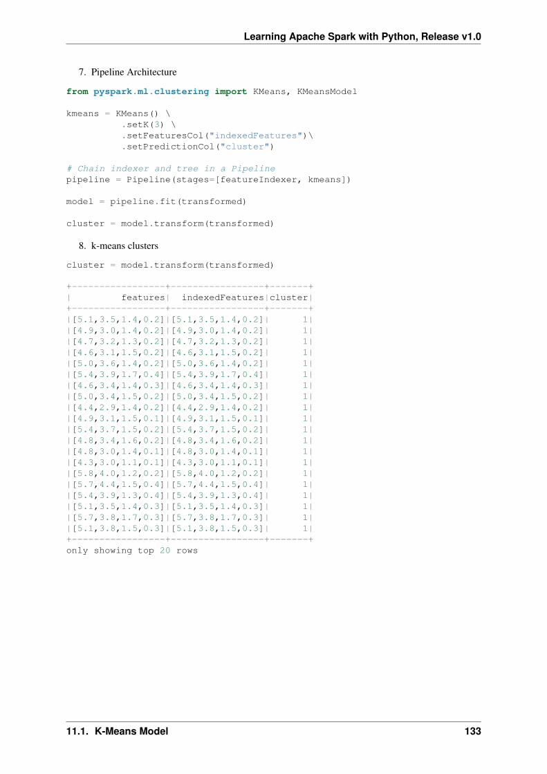
Learning Apache Spark with Python, Release v1.0
7. Pipeline Architecture
from pyspark.ml.clustering import KMeans, KMeansModel
kmeans = KMeans() \.setK(3) \.setFeaturesCol("indexedFeatures")\.setPredictionCol("cluster")
# Chain indexer and tree in a Pipelinepipeline = Pipeline(stages=[featureIndexer, kmeans])
model = pipeline.fit(transformed)
cluster = model.transform(transformed)
8. k-means clusters
cluster = model.transform(transformed)
+-----------------+-----------------+-------+| features| indexedFeatures|cluster|+-----------------+-----------------+-------+|[5.1,3.5,1.4,0.2]|[5.1,3.5,1.4,0.2]| 1||[4.9,3.0,1.4,0.2]|[4.9,3.0,1.4,0.2]| 1||[4.7,3.2,1.3,0.2]|[4.7,3.2,1.3,0.2]| 1||[4.6,3.1,1.5,0.2]|[4.6,3.1,1.5,0.2]| 1||[5.0,3.6,1.4,0.2]|[5.0,3.6,1.4,0.2]| 1||[5.4,3.9,1.7,0.4]|[5.4,3.9,1.7,0.4]| 1||[4.6,3.4,1.4,0.3]|[4.6,3.4,1.4,0.3]| 1||[5.0,3.4,1.5,0.2]|[5.0,3.4,1.5,0.2]| 1||[4.4,2.9,1.4,0.2]|[4.4,2.9,1.4,0.2]| 1||[4.9,3.1,1.5,0.1]|[4.9,3.1,1.5,0.1]| 1||[5.4,3.7,1.5,0.2]|[5.4,3.7,1.5,0.2]| 1||[4.8,3.4,1.6,0.2]|[4.8,3.4,1.6,0.2]| 1||[4.8,3.0,1.4,0.1]|[4.8,3.0,1.4,0.1]| 1||[4.3,3.0,1.1,0.1]|[4.3,3.0,1.1,0.1]| 1||[5.8,4.0,1.2,0.2]|[5.8,4.0,1.2,0.2]| 1||[5.7,4.4,1.5,0.4]|[5.7,4.4,1.5,0.4]| 1||[5.4,3.9,1.3,0.4]|[5.4,3.9,1.3,0.4]| 1||[5.1,3.5,1.4,0.3]|[5.1,3.5,1.4,0.3]| 1||[5.7,3.8,1.7,0.3]|[5.7,3.8,1.7,0.3]| 1||[5.1,3.8,1.5,0.3]|[5.1,3.8,1.5,0.3]| 1|+-----------------+-----------------+-------+only showing top 20 rows
11.1. K-Means Model 133
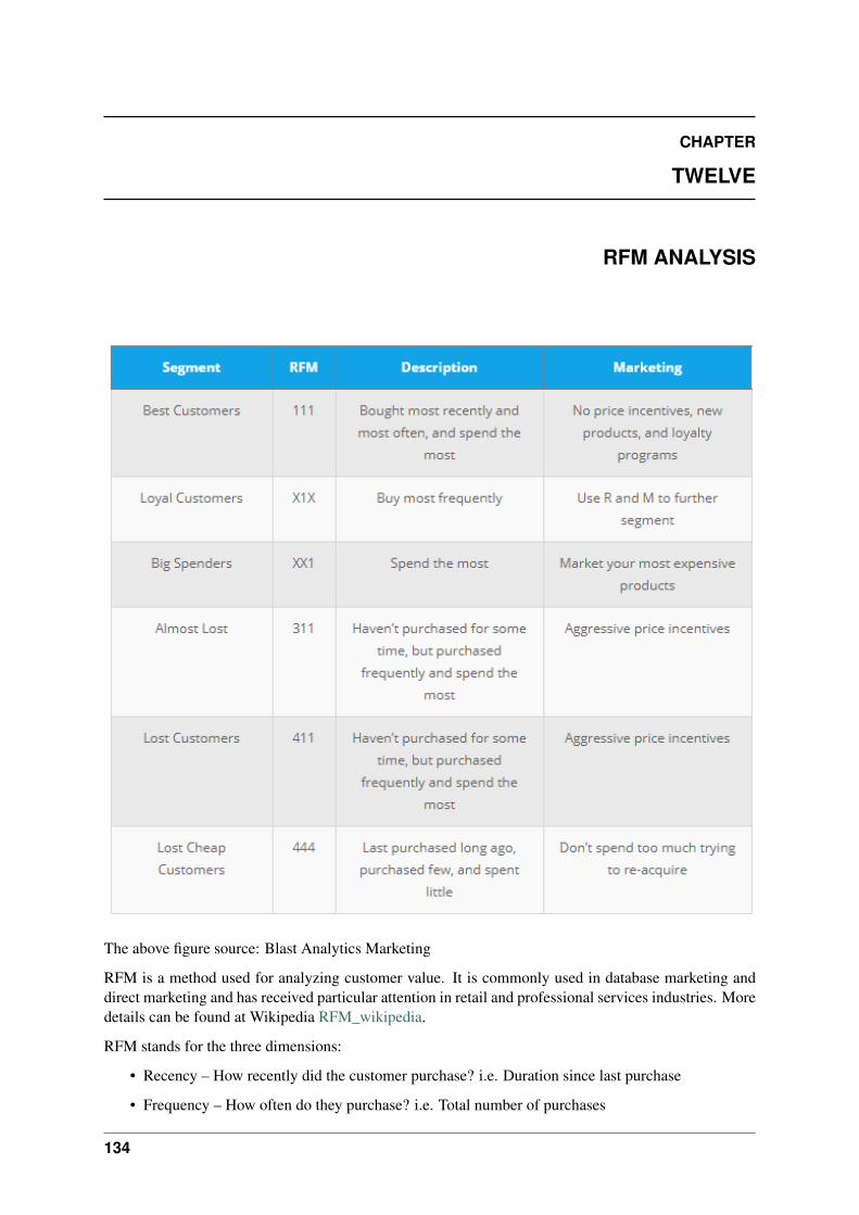
CHAPTER
TWELVE
RFM ANALYSIS
The above figure source: Blast Analytics Marketing
RFM is a method used for analyzing customer value. It is commonly used in database marketing anddirect marketing and has received particular attention in retail and professional services industries. Moredetails can be found at Wikipedia RFM_wikipedia.
RFM stands for the three dimensions:
• Recency – How recently did the customer purchase? i.e. Duration since last purchase
• Frequency – How often do they purchase? i.e. Total number of purchases
134
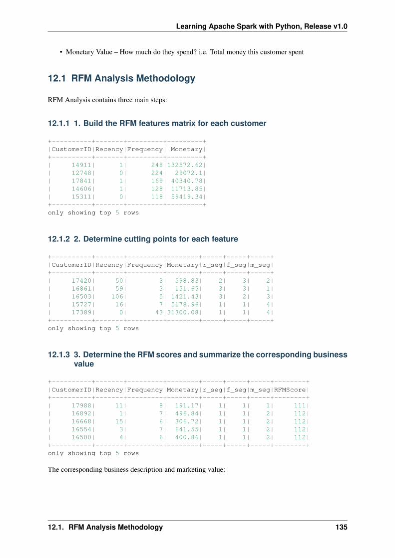
Learning Apache Spark with Python, Release v1.0
• Monetary Value – How much do they spend? i.e. Total money this customer spent
12.1 RFM Analysis Methodology
RFM Analysis contains three main steps:
12.1.1 1. Build the RFM features matrix for each customer
+----------+-------+---------+---------+|CustomerID|Recency|Frequency| Monetary|+----------+-------+---------+---------+| 14911| 1| 248|132572.62|| 12748| 0| 224| 29072.1|| 17841| 1| 169| 40340.78|| 14606| 1| 128| 11713.85|| 15311| 0| 118| 59419.34|+----------+-------+---------+---------+only showing top 5 rows
12.1.2 2. Determine cutting points for each feature
+----------+-------+---------+--------+-----+-----+-----+|CustomerID|Recency|Frequency|Monetary|r_seg|f_seg|m_seg|+----------+-------+---------+--------+-----+-----+-----+| 17420| 50| 3| 598.83| 2| 3| 2|| 16861| 59| 3| 151.65| 3| 3| 1|| 16503| 106| 5| 1421.43| 3| 2| 3|| 15727| 16| 7| 5178.96| 1| 1| 4|| 17389| 0| 43|31300.08| 1| 1| 4|+----------+-------+---------+--------+-----+-----+-----+only showing top 5 rows
12.1.3 3. Determine the RFM scores and summarize the corresponding businessvalue
+----------+-------+---------+--------+-----+-----+-----+--------+|CustomerID|Recency|Frequency|Monetary|r_seg|f_seg|m_seg|RFMScore|+----------+-------+---------+--------+-----+-----+-----+--------+| 17988| 11| 8| 191.17| 1| 1| 1| 111|| 16892| 1| 7| 496.84| 1| 1| 2| 112|| 16668| 15| 6| 306.72| 1| 1| 2| 112|| 16554| 3| 7| 641.55| 1| 1| 2| 112|| 16500| 4| 6| 400.86| 1| 1| 2| 112|+----------+-------+---------+--------+-----+-----+-----+--------+only showing top 5 rows
The corresponding business description and marketing value:
12.1. RFM Analysis Methodology 135
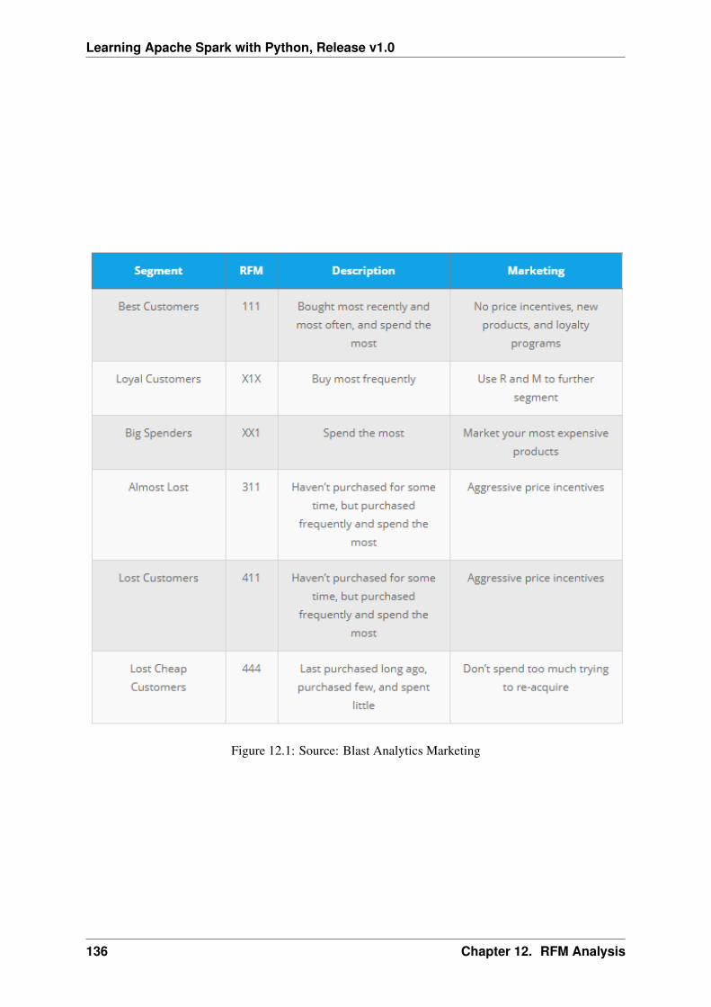
Learning Apache Spark with Python, Release v1.0
Figure 12.1: Source: Blast Analytics Marketing
136 Chapter 12. RFM Analysis
Learning Apache Spark with Python, Release v1.0
12.2 Demo
• The Jupyter notebook can be download from Data Exploration.
• The data can be downloaf from German Credit.
12.2.1 Load and clean data
1. Set up spark context and SparkSession
from pyspark.sql import SparkSession
spark = SparkSession \.builder \.appName("Python Spark RFM example") \.config("spark.some.config.option", "some-value") \.getOrCreate()
2. Load dataset
df_raw = spark.read.format(’com.databricks.spark.csv’).\options(header=’true’, \inferschema=’true’).\
load("Online Retail.csv",header=True);
check the data set
df_raw.show(5)df_raw.printSchema()
Then you will get
+---------+---------+--------------------+--------+------------+---------+----------+--------------+|InvoiceNo|StockCode| Description|Quantity| InvoiceDate|UnitPrice|CustomerID| Country|+---------+---------+--------------------+--------+------------+---------+----------+--------------+| 536365| 85123A|WHITE HANGING HEA...| 6|12/1/10 8:26| 2.55| 17850|United Kingdom|| 536365| 71053| WHITE METAL LANTERN| 6|12/1/10 8:26| 3.39| 17850|United Kingdom|| 536365| 84406B|CREAM CUPID HEART...| 8|12/1/10 8:26| 2.75| 17850|United Kingdom|| 536365| 84029G|KNITTED UNION FLA...| 6|12/1/10 8:26| 3.39| 17850|United Kingdom|| 536365| 84029E|RED WOOLLY HOTTIE...| 6|12/1/10 8:26| 3.39| 17850|United Kingdom|+---------+---------+--------------------+--------+------------+---------+----------+--------------+only showing top 5 rows
root|-- InvoiceNo: string (nullable = true)|-- StockCode: string (nullable = true)|-- Description: string (nullable = true)|-- Quantity: integer (nullable = true)|-- InvoiceDate: string (nullable = true)|-- UnitPrice: double (nullable = true)|-- CustomerID: integer (nullable = true)|-- Country: string (nullable = true)
3. Data clean and data manipulation
• check and remove the null values
12.2. Demo 137
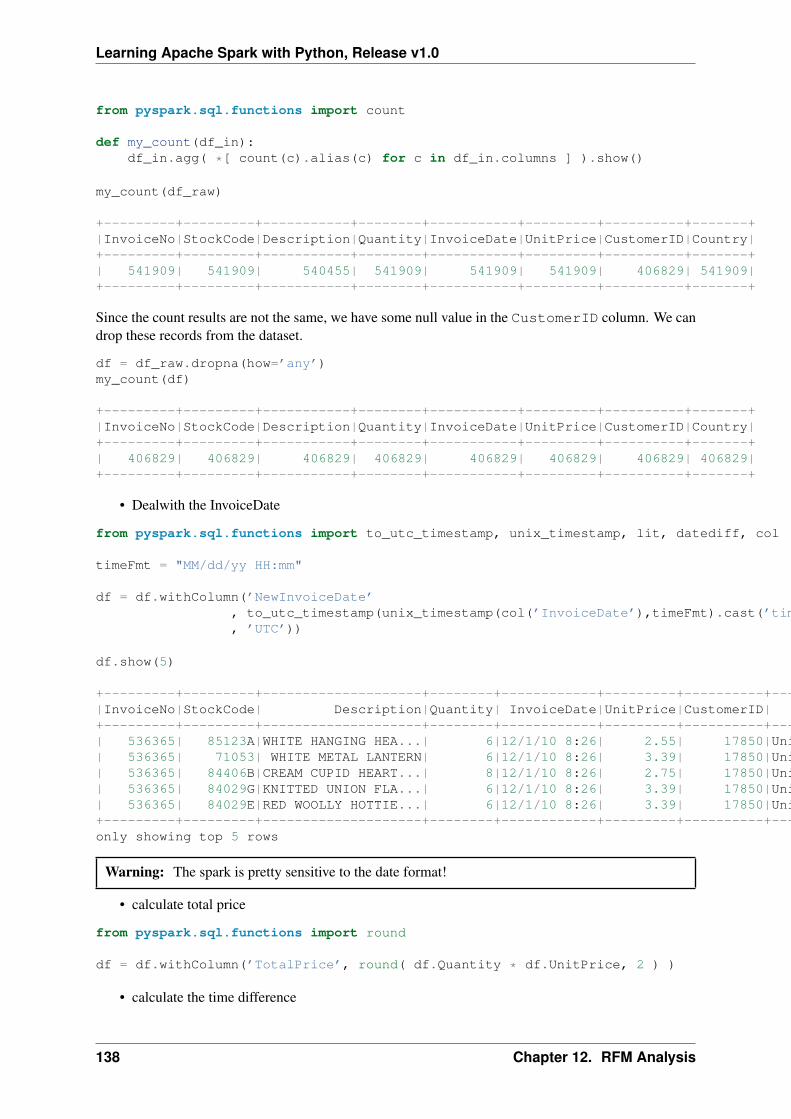
Learning Apache Spark with Python, Release v1.0
from pyspark.sql.functions import count
def my_count(df_in):df_in.agg( *[ count(c).alias(c) for c in df_in.columns ] ).show()
my_count(df_raw)
+---------+---------+-----------+--------+-----------+---------+----------+-------+|InvoiceNo|StockCode|Description|Quantity|InvoiceDate|UnitPrice|CustomerID|Country|+---------+---------+-----------+--------+-----------+---------+----------+-------+| 541909| 541909| 540455| 541909| 541909| 541909| 406829| 541909|+---------+---------+-----------+--------+-----------+---------+----------+-------+
Since the count results are not the same, we have some null value in the CustomerID column. We candrop these records from the dataset.
df = df_raw.dropna(how=’any’)my_count(df)
+---------+---------+-----------+--------+-----------+---------+----------+-------+|InvoiceNo|StockCode|Description|Quantity|InvoiceDate|UnitPrice|CustomerID|Country|+---------+---------+-----------+--------+-----------+---------+----------+-------+| 406829| 406829| 406829| 406829| 406829| 406829| 406829| 406829|+---------+---------+-----------+--------+-----------+---------+----------+-------+
• Dealwith the InvoiceDate
from pyspark.sql.functions import to_utc_timestamp, unix_timestamp, lit, datediff, col
timeFmt = "MM/dd/yy HH:mm"
df = df.withColumn(’NewInvoiceDate’, to_utc_timestamp(unix_timestamp(col(’InvoiceDate’),timeFmt).cast(’timestamp’), ’UTC’))
df.show(5)
+---------+---------+--------------------+--------+------------+---------+----------+--------------+--------------------+|InvoiceNo|StockCode| Description|Quantity| InvoiceDate|UnitPrice|CustomerID| Country| NewInvoiceDate|+---------+---------+--------------------+--------+------------+---------+----------+--------------+--------------------+| 536365| 85123A|WHITE HANGING HEA...| 6|12/1/10 8:26| 2.55| 17850|United Kingdom|2010-12-01 08:26:...|| 536365| 71053| WHITE METAL LANTERN| 6|12/1/10 8:26| 3.39| 17850|United Kingdom|2010-12-01 08:26:...|| 536365| 84406B|CREAM CUPID HEART...| 8|12/1/10 8:26| 2.75| 17850|United Kingdom|2010-12-01 08:26:...|| 536365| 84029G|KNITTED UNION FLA...| 6|12/1/10 8:26| 3.39| 17850|United Kingdom|2010-12-01 08:26:...|| 536365| 84029E|RED WOOLLY HOTTIE...| 6|12/1/10 8:26| 3.39| 17850|United Kingdom|2010-12-01 08:26:...|+---------+---------+--------------------+--------+------------+---------+----------+--------------+--------------------+only showing top 5 rows
Warning: The spark is pretty sensitive to the date format!
• calculate total price
from pyspark.sql.functions import round
df = df.withColumn(’TotalPrice’, round( df.Quantity * df.UnitPrice, 2 ) )
• calculate the time difference
138 Chapter 12. RFM Analysis
Learning Apache Spark with Python, Release v1.0
from pyspark.sql.functions import mean, min, max, sum, datediff, to_date
date_max = df.select(max(’NewInvoiceDate’)).toPandas()current = to_utc_timestamp( unix_timestamp(lit(str(date_max.iloc[0][0])), \
’yy-MM-dd HH:mm’).cast(’timestamp’), ’UTC’ )
# Calculatre Durationdf = df.withColumn(’Duration’, datediff(lit(current), ’NewInvoiceDate’))
• build the Recency, Frequency and Monetary
recency = df.groupBy(’CustomerID’).agg(min(’Duration’).alias(’Recency’))frequency = df.groupBy(’CustomerID’, ’InvoiceNo’).count()\
.groupBy(’CustomerID’)\
.agg(count("*").alias("Frequency"))monetary = df.groupBy(’CustomerID’).agg(round(sum(’TotalPrice’), 2).alias(’Monetary’))rfm = recency.join(frequency,’CustomerID’, how = ’inner’)\
.join(monetary,’CustomerID’, how = ’inner’)
rfm.show(5)
+----------+-------+---------+--------+|CustomerID|Recency|Frequency|Monetary|+----------+-------+---------+--------+| 17420| 50| 3| 598.83|| 16861| 59| 3| 151.65|| 16503| 106| 5| 1421.43|| 15727| 16| 7| 5178.96|| 17389| 0| 43|31300.08|+----------+-------+---------+--------+only showing top 5 rows
12.2.2 RFM Segmentation
4. Determine cutting points
In this section, you can use the techniques (statistical results and visualizations) in Data Explorationsection to help you determine the cutting points for each attribute. In my opinion, the cutting points aremainly depend on the business sense. You’s better talk to your makrting people and get feedback andsuggestion from them. I will use the quantile as the cutting points in this demo.
cols = [’Recency’,’Frequency’,’Monetary’]describe_pd(rfm,cols,1)
+-------+-----------------+-----------------+------------------+|summary| Recency| Frequency| Monetary|+-------+-----------------+-----------------+------------------+| count| 4372.0| 4372.0| 4372.0|| mean|91.58119853613907| 5.07548032936871|1898.4597003659655|| stddev|100.7721393138483|9.338754163574727| 8219.345141139722|| min| 0.0| 1.0| -4287.63|| max| 373.0| 248.0| 279489.02|| 25%| 16.0| 1.0|293.36249999999995|| 50%| 50.0| 3.0| 648.075|| 75%| 143.0| 5.0| 1611.725|+-------+-----------------+-----------------+------------------+
12.2. Demo 139
Learning Apache Spark with Python, Release v1.0
The user defined function by using the cutting points:
def RScore(x):if x <= 16:
return 1elif x<= 50:
return 2elif x<= 143:
return 3else:
return 4
def FScore(x):if x <= 1:
return 4elif x <= 3:
return 3elif x <= 5:
return 2else:
return 1
def MScore(x):if x <= 293:
return 4elif x <= 648:
return 3elif x <= 1611:
return 2else:
return 1
from pyspark.sql.functions import udffrom pyspark.sql.types import StringType, DoubleType
R_udf = udf(lambda x: RScore(x), StringType())F_udf = udf(lambda x: FScore(x), StringType())M_udf = udf(lambda x: MScore(x), StringType())
5. RFM Segmentation
rfm_seg = rfm.withColumn("r_seg", R_udf("Recency"))rfm_seg = rfm_seg.withColumn("f_seg", F_udf("Frequency"))rfm_seg = rfm_seg.withColumn("m_seg", M_udf("Monetary"))rfm_seg = rfm_seg.withColumn(’RFMScore’,
F.concat(F.col(’r_seg’),F.col(’f_seg’), F.col(’m_seg’)))rfm_seg.sort(F.col(’RFMScore’)).show(5)
12.2.3 Statistical Summary
6. Statistical Summary
• simple summary
rfm_seg.groupBy(’RFMScore’)\.agg({’Recency’:’mean’,
’Frequency’: ’mean’,
140 Chapter 12. RFM Analysis
Learning Apache Spark with Python, Release v1.0
’Monetary’: ’mean’} )\.sort(F.col(’RFMScore’)).show(5)
+--------+-----------------+------------------+------------------+|RFMScore| avg(Recency)| avg(Monetary)| avg(Frequency)|+--------+-----------------+------------------+------------------+| 111| 11.0| 191.17| 8.0|| 112| 8.0| 505.9775| 7.5|| 113|7.237113402061856|1223.3604123711339| 7.752577319587629|| 114|6.035123966942149| 8828.888595041324|18.882231404958677|| 121| 9.6| 207.24| 4.4|+--------+-----------------+------------------+------------------+only showing top 5 rows
• complex summary
grp = ’RFMScore’num_cols = [’Recency’,’Frequency’,’Monetary’]df_input = rfm_seg
quantile_grouped = quantile_agg(df_input,grp,num_cols)quantile_grouped.toPandas().to_csv(output_dir+’quantile_grouped.csv’)
deciles_grouped = deciles_agg(df_input,grp,num_cols)deciles_grouped.toPandas().to_csv(output_dir+’deciles_grouped.csv’)
12.3 Extension
You can also apply the K-means clustering in Clustering section to do the segmentation.
12.3.1 Build feature matrix
1. build dense feature matrix
from pyspark.sql import Rowfrom pyspark.ml.linalg import Vectors
# method 1 (good for small feature):#def transData(row):# return Row(label=row["Sales"],# features=Vectors.dense([row["TV"],# row["Radio"],# row["Newspaper"]]))
# Method 2 (good for large features):def transData(data):
return data.rdd.map(lambda r: [r[0],Vectors.dense(r[1:])]).toDF([’CustomerID’,’rfm’])
transformed= transData(rfm)transformed.show(5)
+----------+-------------------+|CustomerID| rfm|+----------+-------------------+
12.3. Extension 141
Learning Apache Spark with Python, Release v1.0
| 17420| [50.0,3.0,598.83]|| 16861| [59.0,3.0,151.65]|| 16503|[106.0,5.0,1421.43]|| 15727| [16.0,7.0,5178.96]|| 17389|[0.0,43.0,31300.08]|+----------+-------------------+only showing top 5 rows
2. Scaler the feature matrix
from pyspark.ml.feature import MinMaxScaler
scaler = MinMaxScaler(inputCol="rfm",\outputCol="features")
scalerModel = scaler.fit(transformed)scaledData = scalerModel.transform(transformed)scaledData.show(5,False)
+----------+-------------------+--------------------------------------------------------------+|CustomerID|rfm |features |+----------+-------------------+--------------------------------------------------------------+|17420 |[50.0,3.0,598.83] |[0.13404825737265416,0.008097165991902834,0.01721938714830836]||16861 |[59.0,3.0,151.65] |[0.1581769436997319,0.008097165991902834,0.01564357039241953] ||16503 |[106.0,5.0,1421.43]|[0.28418230563002683,0.016194331983805668,0.02011814573186342]||15727 |[16.0,7.0,5178.96] |[0.04289544235924933,0.024291497975708502,0.03335929858922501]||17389 |[0.0,43.0,31300.08]|[0.0,0.1700404858299595,0.12540746393334334] |+----------+-------------------+--------------------------------------------------------------+only showing top 5 rows
12.3.2 K-means clustering
3. Find optimal number of cluster
I will present two popular ways to determine the optimal number of the cluster.
• elbow analysis
#PySpark librariesfrom pyspark.ml import Pipelinefrom pyspark.ml.feature import StringIndexer, OneHotEncoder, VectorAssemblerfrom pyspark.sql.functions import col, percent_rank, litfrom pyspark.sql.window import Windowfrom pyspark.sql import DataFrame, Rowfrom pyspark.sql.types import StructTypefrom functools import reduce # For Python 3.x
from pyspark.ml.clustering import KMeans#from pyspark.ml.evaluation import ClusteringEvaluator # requires Spark 2.4 or later
import numpy as npcost = np.zeros(20)for k in range(2,20):
kmeans = KMeans()\.setK(k)\.setSeed(1) \.setFeaturesCol("features")\.setPredictionCol("cluster")
142 Chapter 12. RFM Analysis
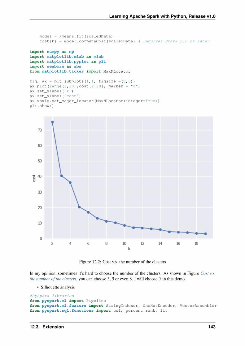
Learning Apache Spark with Python, Release v1.0
model = kmeans.fit(scaledData)cost[k] = model.computeCost(scaledData) # requires Spark 2.0 or later
import numpy as npimport matplotlib.mlab as mlabimport matplotlib.pyplot as pltimport seaborn as sbsfrom matplotlib.ticker import MaxNLocator
fig, ax = plt.subplots(1,1, figsize =(8,6))ax.plot(range(2,20),cost[2:20], marker = "o")ax.set_xlabel(’k’)ax.set_ylabel(’cost’)ax.xaxis.set_major_locator(MaxNLocator(integer=True))plt.show()
Figure 12.2: Cost v.s. the number of the clusters
In my opinion, sometimes it’s hard to choose the number of the clusters. As shown in Figure Cost v.s.the number of the clusters, you can choose 3, 5 or even 8. I will choose 3 in this demo.
• Silhouette analysis
#PySpark librariesfrom pyspark.ml import Pipelinefrom pyspark.ml.feature import StringIndexer, OneHotEncoder, VectorAssemblerfrom pyspark.sql.functions import col, percent_rank, lit
12.3. Extension 143
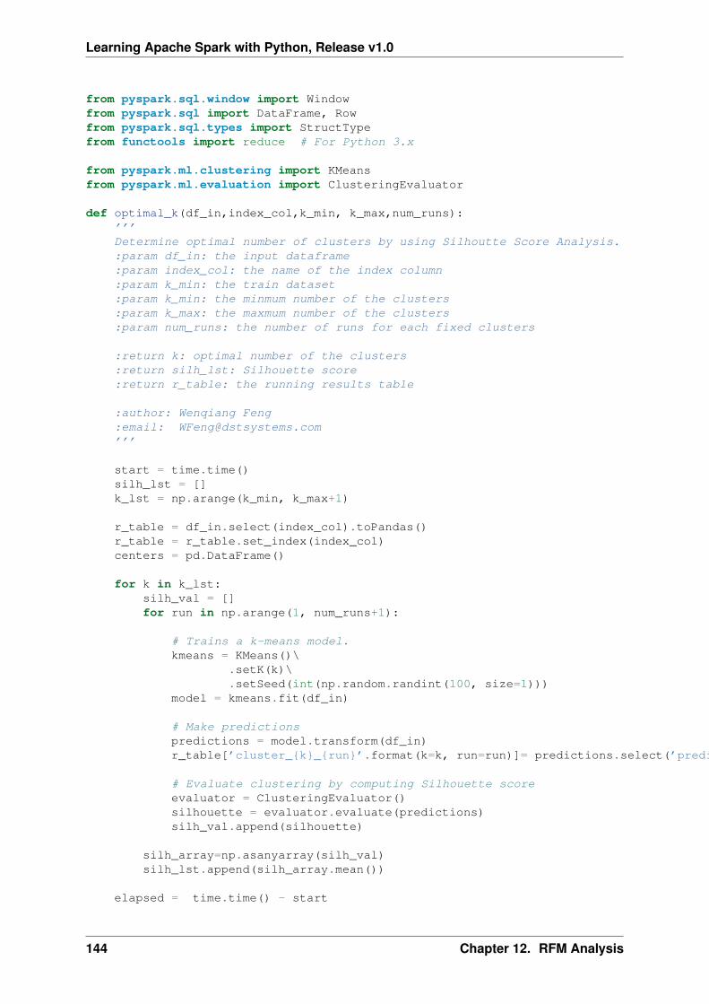
Learning Apache Spark with Python, Release v1.0
from pyspark.sql.window import Windowfrom pyspark.sql import DataFrame, Rowfrom pyspark.sql.types import StructTypefrom functools import reduce # For Python 3.x
from pyspark.ml.clustering import KMeansfrom pyspark.ml.evaluation import ClusteringEvaluator
def optimal_k(df_in,index_col,k_min, k_max,num_runs):’’’Determine optimal number of clusters by using Silhoutte Score Analysis.:param df_in: the input dataframe:param index_col: the name of the index column:param k_min: the train dataset:param k_min: the minmum number of the clusters:param k_max: the maxmum number of the clusters:param num_runs: the number of runs for each fixed clusters
:return k: optimal number of the clusters:return silh_lst: Silhouette score:return r_table: the running results table
:author: Wenqiang Feng:email: [email protected]’’’
start = time.time()silh_lst = []k_lst = np.arange(k_min, k_max+1)
r_table = df_in.select(index_col).toPandas()r_table = r_table.set_index(index_col)centers = pd.DataFrame()
for k in k_lst:silh_val = []for run in np.arange(1, num_runs+1):
# Trains a k-means model.kmeans = KMeans()\
.setK(k)\
.setSeed(int(np.random.randint(100, size=1)))model = kmeans.fit(df_in)
# Make predictionspredictions = model.transform(df_in)r_table[’cluster_{k}_{run}’.format(k=k, run=run)]= predictions.select(’prediction’).toPandas()
# Evaluate clustering by computing Silhouette scoreevaluator = ClusteringEvaluator()silhouette = evaluator.evaluate(predictions)silh_val.append(silhouette)
silh_array=np.asanyarray(silh_val)silh_lst.append(silh_array.mean())
elapsed = time.time() - start
144 Chapter 12. RFM Analysis
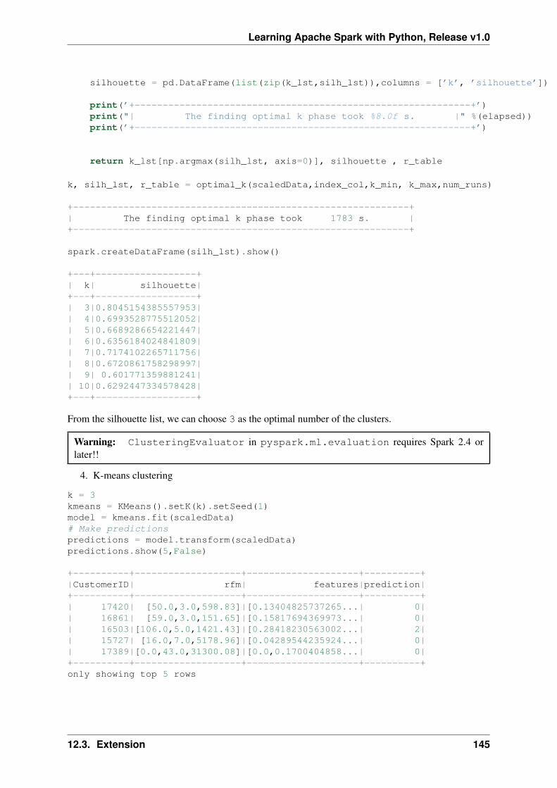
Learning Apache Spark with Python, Release v1.0
silhouette = pd.DataFrame(list(zip(k_lst,silh_lst)),columns = [’k’, ’silhouette’])
print(’+------------------------------------------------------------+’)print("| The finding optimal k phase took %8.0f s. |" %(elapsed))print(’+------------------------------------------------------------+’)
return k_lst[np.argmax(silh_lst, axis=0)], silhouette , r_table
k, silh_lst, r_table = optimal_k(scaledData,index_col,k_min, k_max,num_runs)
+------------------------------------------------------------+| The finding optimal k phase took 1783 s. |+------------------------------------------------------------+
spark.createDataFrame(silh_lst).show()
+---+------------------+| k| silhouette|+---+------------------+| 3|0.8045154385557953|| 4|0.6993528775512052|| 5|0.6689286654221447|| 6|0.6356184024841809|| 7|0.7174102265711756|| 8|0.6720861758298997|| 9| 0.601771359881241|| 10|0.6292447334578428|+---+------------------+
From the silhouette list, we can choose 3 as the optimal number of the clusters.
Warning: ClusteringEvaluator in pyspark.ml.evaluation requires Spark 2.4 orlater!!
4. K-means clustering
k = 3kmeans = KMeans().setK(k).setSeed(1)model = kmeans.fit(scaledData)# Make predictionspredictions = model.transform(scaledData)predictions.show(5,False)
+----------+-------------------+--------------------+----------+|CustomerID| rfm| features|prediction|+----------+-------------------+--------------------+----------+| 17420| [50.0,3.0,598.83]|[0.13404825737265...| 0|| 16861| [59.0,3.0,151.65]|[0.15817694369973...| 0|| 16503|[106.0,5.0,1421.43]|[0.28418230563002...| 2|| 15727| [16.0,7.0,5178.96]|[0.04289544235924...| 0|| 17389|[0.0,43.0,31300.08]|[0.0,0.1700404858...| 0|+----------+-------------------+--------------------+----------+only showing top 5 rows
12.3. Extension 145
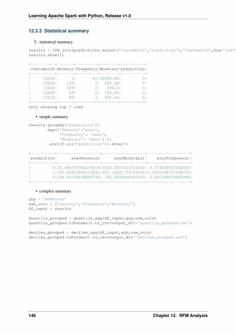
Learning Apache Spark with Python, Release v1.0
12.3.3 Statistical summary
5. statistical summary
results = rfm.join(predictions.select(’CustomerID’,’prediction’),’CustomerID’,how=’left’)results.show(5)
+----------+-------+---------+--------+----------+|CustomerID|Recency|Frequency|Monetary|prediction|+----------+-------+---------+--------+----------+| 13098| 1| 41|28658.88| 0|| 13248| 124| 2| 465.68| 2|| 13452| 259| 2| 590.0| 1|| 13460| 29| 2| 183.44| 0|| 13518| 85| 1| 659.44| 0|+----------+-------+---------+--------+----------+only showing top 5 rows
• simple summary
results.groupBy(’prediction’)\.agg({’Recency’:’mean’,
’Frequency’: ’mean’,’Monetary’: ’mean’} )\
.sort(F.col(’prediction’)).show(5)
+----------+------------------+------------------+------------------+|prediction| avg(Recency)| avg(Monetary)| avg(Frequency)|+----------+------------------+------------------+------------------+| 0|30.966337980278816|2543.0355321319284| 6.514450867052023|| 1|296.02403846153845|407.16831730769206|1.5592948717948718|| 2|154.40148698884758| 702.5096406443623| 2.550185873605948|+----------+------------------+------------------+------------------+
• complex summary
grp = ’RFMScore’num_cols = [’Recency’,’Frequency’,’Monetary’]df_input = results
quantile_grouped = quantile_agg(df_input,grp,num_cols)quantile_grouped.toPandas().to_csv(output_dir+’quantile_grouped.csv’)
deciles_grouped = deciles_agg(df_input,grp,num_cols)deciles_grouped.toPandas().to_csv(output_dir+’deciles_grouped.csv’)
146 Chapter 12. RFM Analysis
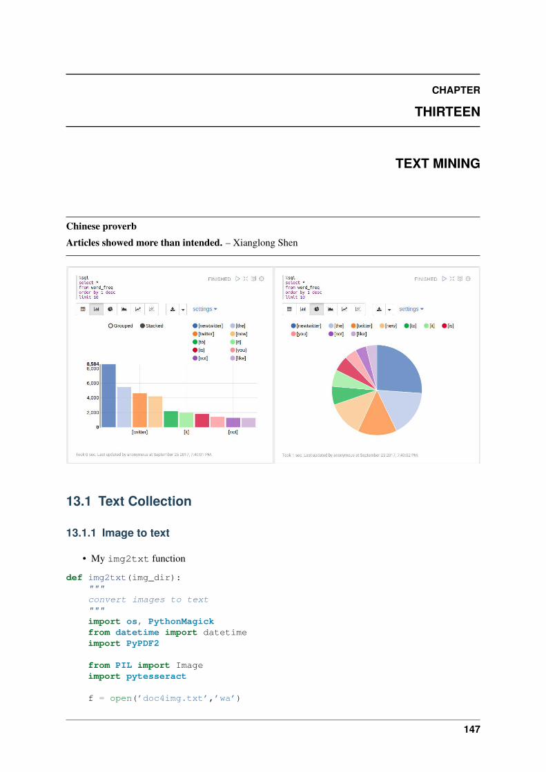
CHAPTER
THIRTEEN
TEXT MINING
Chinese proverb
Articles showed more than intended. – Xianglong Shen
13.1 Text Collection
13.1.1 Image to text
• My img2txt function
def img2txt(img_dir):"""convert images to text"""import os, PythonMagickfrom datetime import datetimeimport PyPDF2
from PIL import Imageimport pytesseract
f = open(’doc4img.txt’,’wa’)
147
Learning Apache Spark with Python, Release v1.0
for img in [img_file for img_file in os.listdir(img_dir)if (img_file.endswith(".png") or
img_file.endswith(".jpg") orimg_file.endswith(".jpeg"))]:
start_time = datetime.now()
input_img = img_dir + "/" + img
print(’--------------------------------------------------------------------’)print(img)print(’Converting ’ + img +’.......’)print(’--------------------------------------------------------------------’)
# extract the text information from imagestext = pytesseract.image_to_string(Image.open(input_img))print(text)
# ouput text filef.write( img + "\n")f.write(text.encode(’utf-8’))
print "CPU Time for converting" + img +":"+ str(datetime.now() - start_time) +"\n"f.write( "\n-------------------------------------------------------------\n")
f.close()
• Demo
I applied my img2txt function to the image in Image folder.
image_dir = r"Image"
img2txt(image_dir)
Then I got the following results:
--------------------------------------------------------------------feng.pdf_0.pngConverting feng.pdf_0.png.......--------------------------------------------------------------------l I l w
Wenqiang FengData ScientistDST APPLIED ANALYTICS GROUP
Wenqiang Feng is Data Scientist for DST’s Applied Analytics Group. Dr. Feng’s responsibilitiesinclude providing DST clients with access to cutting--edge skills and technologies, including BigData analytic solutions, advanced analytic and data enhancement techniques and modeling.
Dr. Feng has deep analytic expertise in data mining, analytic systems, machine learningalgorithms, business intelligence, and applying Big Data tools to strategically solve industryproblems in a cross--functional business. Before joining the DST Applied Analytics Group, Dr.Feng holds a MA Data Science Fellow at The Institute for Mathematics and Its Applications
148 Chapter 13. Text Mining
Learning Apache Spark with Python, Release v1.0
{IMA) at the University of Minnesota. While there, he helped startup companies makemarketing decisions based on deep predictive analytics.
Dr. Feng graduated from University of Tennessee, Knoxville with PhD in Computationalmathematics and Master’s degree in Statistics. He also holds Master’s degree in ComputationalMathematics at Missouri University of Science and Technology (MST) and Master’s degree inApplied Mathematics at University of science and technology of China (USTC).CPU Time for convertingfeng.pdf_0.png:0:00:02.061208
13.1.2 Image Enhnaced to text
• My img2txt_enhance function
def img2txt_enhance(img_dir,scaler):"""convert images files to text"""
import numpy as npimport os, PythonMagickfrom datetime import datetimeimport PyPDF2
from PIL import Image, ImageEnhance, ImageFilterimport pytesseract
f = open(’doc4img.txt’,’wa’)for img in [img_file for img_file in os.listdir(img_dir)
if (img_file.endswith(".png") orimg_file.endswith(".jpg") orimg_file.endswith(".jpeg"))]:
start_time = datetime.now()
input_img = img_dir + "/" + imgenhanced_img = img_dir + "/" +"Enhanced" + "/"+ img
im = Image.open(input_img) # the second oneim = im.filter(ImageFilter.MedianFilter())enhancer = ImageEnhance.Contrast(im)im = enhancer.enhance(1)im = im.convert(’1’)im.save(enhanced_img)
for scale in np.ones(scaler):im = Image.open(enhanced_img) # the second oneim = im.filter(ImageFilter.MedianFilter())enhancer = ImageEnhance.Contrast(im)im = enhancer.enhance(scale)im = im.convert(’1’)im.save(enhanced_img)
print(’--------------------------------------------------------------------’)print(img)
13.1. Text Collection 149
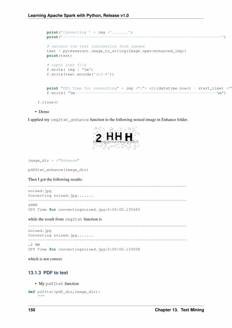
Learning Apache Spark with Python, Release v1.0
print(’Converting ’ + img +’.......’)print(’--------------------------------------------------------------------’)
# extract the text information from imagestext = pytesseract.image_to_string(Image.open(enhanced_img))print(text)
# ouput text filef.write( img + "\n")f.write(text.encode(’utf-8’))
print "CPU Time for converting" + img +":"+ str(datetime.now() - start_time) +"\n"f.write( "\n-------------------------------------------------------------\n")
f.close()
• Demo
I applied my img2txt_enhance function to the following noised image in Enhance folder.
image_dir = r"Enhance"
pdf2txt_enhance(image_dir)
Then I got the following results:
--------------------------------------------------------------------noised.jpgConverting noised.jpg.......--------------------------------------------------------------------zHHHCPU Time for convertingnoised.jpg:0:00:00.135465
while the result from img2txt function is
--------------------------------------------------------------------noised.jpgConverting noised.jpg.......--------------------------------------------------------------------,2 WWCPU Time for convertingnoised.jpg:0:00:00.133508
which is not correct.
13.1.3 PDF to text
• My pdf2txt function
def pdf2txt(pdf_dir,image_dir):"""
150 Chapter 13. Text Mining
Learning Apache Spark with Python, Release v1.0
convert PDF to text"""
import os, PythonMagickfrom datetime import datetimeimport PyPDF2
from PIL import Imageimport pytesseract
f = open(’doc.txt’,’wa’)for pdf in [pdf_file for pdf_file in os.listdir(pdf_dir) if pdf_file.endswith(".pdf")]:
start_time = datetime.now()
input_pdf = pdf_dir + "/" + pdf
pdf_im = PyPDF2.PdfFileReader(file(input_pdf, "rb"))npage = pdf_im.getNumPages()
print(’--------------------------------------------------------------------’)print(pdf)print(’Converting %d pages.’ % npage)print(’--------------------------------------------------------------------’)
f.write( "\n--------------------------------------------------------------------\n")
for p in range(npage):
pdf_file = input_pdf + ’[’ + str(p) +’]’image_file = image_dir + "/" + pdf+ ’_’ + str(p)+ ’.png’
# convert PDF files to Imagesim = PythonMagick.Image()im.density(’300’)im.read(pdf_file)im.write(image_file)
# extract the text information from imagestext = pytesseract.image_to_string(Image.open(image_file))
#print(text)
# ouput text filef.write( pdf + "\n")f.write(text.encode(’utf-8’))
print "CPU Time for converting" + pdf +":"+ str(datetime.now() - start_time) +"\n"
f.close()
• Demo
I applied my pdf2txt function to my scaned bio pdf file in pdf folder.
pdf_dir = r"pdf"image_dir = r"Image"
13.1. Text Collection 151
Learning Apache Spark with Python, Release v1.0
pdf2txt(pdf_dir,image_dir)
Then I got the following results:
--------------------------------------------------------------------feng.pdfConverting 1 pages.--------------------------------------------------------------------l I l w
Wenqiang FengData ScientistDST APPLIED ANALYTICS GROUP
Wenqiang Feng is Data Scientist for DST’s Applied Analytics Group. Dr. Feng’s responsibilitiesinclude providing DST clients with access to cutting--edge skills and technologies, including BigData analytic solutions, advanced analytic and data enhancement techniques and modeling.
Dr. Feng has deep analytic expertise in data mining, analytic systems, machine learningalgorithms, business intelligence, and applying Big Data tools to strategically solve industryproblems in a cross--functional business. Before joining the DST Applied Analytics Group, Dr.Feng holds a MA Data Science Fellow at The Institute for Mathematics and Its Applications{IMA) at the University of Minnesota. While there, he helped startup companies makemarketing decisions based on deep predictive analytics.
Dr. Feng graduated from University of Tennessee, Knoxville with PhD in Computationalmathematics and Master’s degree in Statistics. He also holds Master’s degree in ComputationalMathematics at Missouri University of Science and Technology (MST) and Master’s degree inApplied Mathematics at University of science and technology of China (USTC).CPU Time for convertingfeng.pdf:0:00:03.143800
13.1.4 Audio to text
• My audio2txt function
def audio2txt(audio_dir):’’’ convert audio to text’’’
import speech_recognition as srr = sr.Recognizer()
f = open(’doc.txt’,’wa’)for audio_n in [audio_file for audio_file in os.listdir(audio_dir) \
if audio_file.endswith(".wav")]:
filename = audio_dir + "/" + audio_n
# Read audio datawith sr.AudioFile(filename) as source:
audio = r.record(source) # read the entire audio file
# Google Speech Recognitiontext = r.recognize_google(audio)
152 Chapter 13. Text Mining
Learning Apache Spark with Python, Release v1.0
# ouput text filef.write( audio_n + ": ")f.write(text.encode(’utf-8’))f.write("\n")
print(’You said: ’ + text)
f.close()
• Demo
I applied my audio2txt function to my audio records in audio folder.
audio_dir = r"audio"
audio2txt(audio_dir)
Then I got the following results:
You said: hello this is George welcome to my tutorialYou said: mathematics is important in daily lifeYou said: call me tomorrowYou said: do you want something to eatYou said: I want to speak with himYou said: nice to see youYou said: can you speak slowlyYou said: have a good day
By the way, you can use my following python code to record your own audio and play with audio2txtfunction in Command-line python record.py "demo2.wav":
import sys, getopt
import speech_recognition as sr
audio_filename = sys.argv[1]
r = sr.Recognizer()with sr.Microphone() as source:
r.adjust_for_ambient_noise(source)print("Hey there, say something, I am recording!")audio = r.listen(source)print("Done listening!")
with open(audio_filename, "wb") as f:f.write(audio.get_wav_data())
13.2 Text Preprocessing
• check to see if a row only contains whitespace
def check_blanks(data_str):is_blank = str(data_str.isspace())return is_blank
13.2. Text Preprocessing 153
Learning Apache Spark with Python, Release v1.0
• Determine whether the language of the text content is english or not: Use langid module to classifythe language to make sure we are applying the correct cleanup actions for English langid
def check_lang(data_str):predict_lang = langid.classify(data_str)if predict_lang[1] >= .9:
language = predict_lang[0]else:
language = ’NA’return language
• Remove features
def remove_features(data_str):# compile regexurl_re = re.compile(’https?://(www.)?\w+\.\w+(/\w+)*/?’)punc_re = re.compile(’[%s]’ % re.escape(string.punctuation))num_re = re.compile(’(\\d+)’)mention_re = re.compile(’@(\w+)’)alpha_num_re = re.compile("^[a-z0-9_.]+$")# convert to lowercasedata_str = data_str.lower()# remove hyperlinksdata_str = url_re.sub(’ ’, data_str)# remove @mentionsdata_str = mention_re.sub(’ ’, data_str)# remove puncuationdata_str = punc_re.sub(’ ’, data_str)# remove numeric ’words’data_str = num_re.sub(’ ’, data_str)# remove non a-z 0-9 characters and words shorter than 3 characterslist_pos = 0cleaned_str = ’’for word in data_str.split():
if list_pos == 0:if alpha_num_re.match(word) and len(word) > 2:
cleaned_str = wordelse:
cleaned_str = ’ ’else:
if alpha_num_re.match(word) and len(word) > 2:cleaned_str = cleaned_str + ’ ’ + word
else:cleaned_str += ’ ’
list_pos += 1return cleaned_str
• removes stop words
def remove_stops(data_str):# expects a stringstops = set(stopwords.words("english"))list_pos = 0cleaned_str = ’’text = data_str.split()for word in text:
if word not in stops:# rebuild cleaned_str
154 Chapter 13. Text Mining
Learning Apache Spark with Python, Release v1.0
if list_pos == 0:cleaned_str = word
else:cleaned_str = cleaned_str + ’ ’ + word
list_pos += 1return cleaned_str
• tagging text
def tag_and_remove(data_str):cleaned_str = ’ ’# noun tagsnn_tags = [’NN’, ’NNP’, ’NNP’, ’NNPS’, ’NNS’]# adjectivesjj_tags = [’JJ’, ’JJR’, ’JJS’]# verbsvb_tags = [’VB’, ’VBD’, ’VBG’, ’VBN’, ’VBP’, ’VBZ’]nltk_tags = nn_tags + jj_tags + vb_tags
# break string into ’words’text = data_str.split()
# tag the text and keep only those with the right tagstagged_text = pos_tag(text)for tagged_word in tagged_text:
if tagged_word[1] in nltk_tags:cleaned_str += tagged_word[0] + ’ ’
return cleaned_str
• lemmatization
def lemmatize(data_str):# expects a stringlist_pos = 0cleaned_str = ’’lmtzr = WordNetLemmatizer()text = data_str.split()tagged_words = pos_tag(text)for word in tagged_words:
if ’v’ in word[1].lower():lemma = lmtzr.lemmatize(word[0], pos=’v’)
else:lemma = lmtzr.lemmatize(word[0], pos=’n’)
if list_pos == 0:cleaned_str = lemma
else:cleaned_str = cleaned_str + ’ ’ + lemma
list_pos += 1return cleaned_str
define the preprocessing function in PySpark
from pyspark.sql.functions import udffrom pyspark.sql.types import StringTypeimport preproc as pp
check_lang_udf = udf(pp.check_lang, StringType())
13.2. Text Preprocessing 155
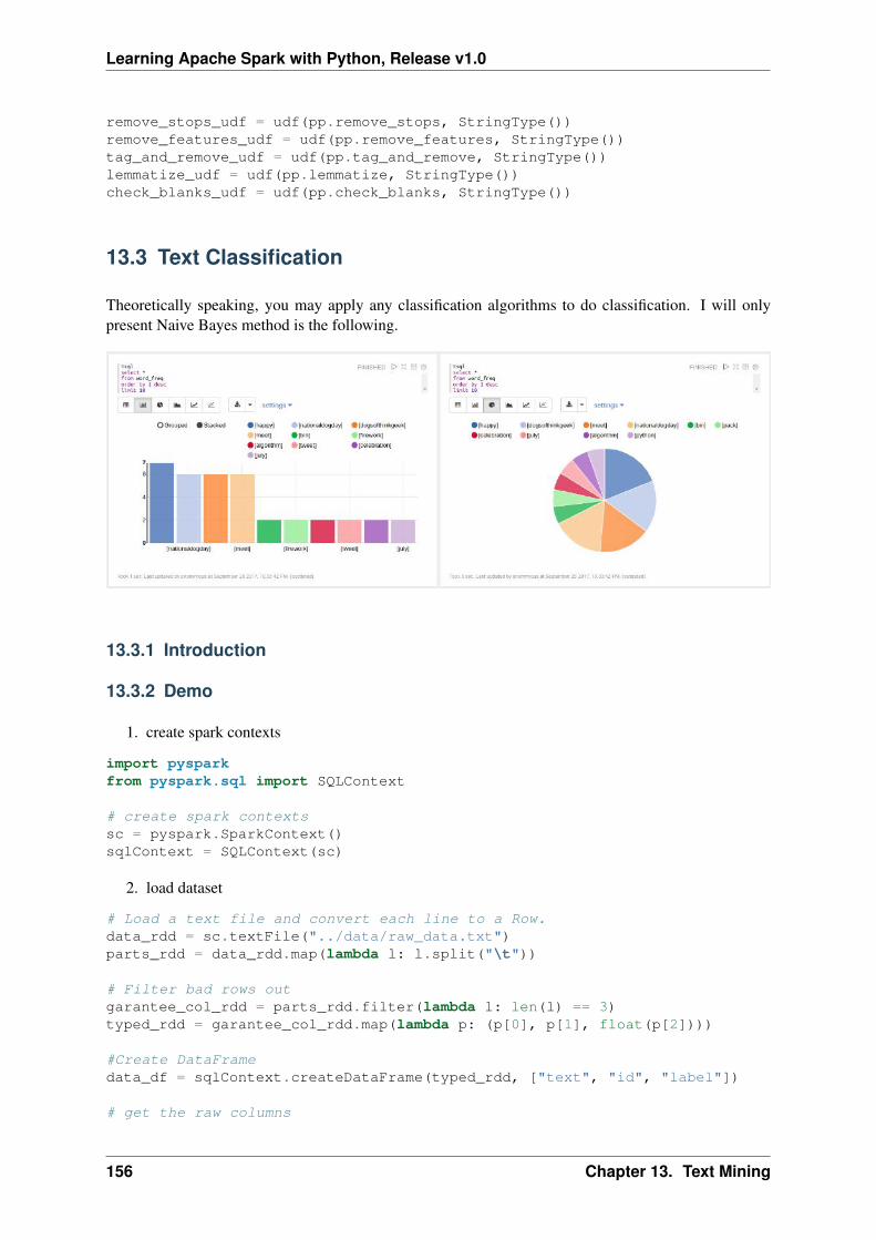
Learning Apache Spark with Python, Release v1.0
remove_stops_udf = udf(pp.remove_stops, StringType())remove_features_udf = udf(pp.remove_features, StringType())tag_and_remove_udf = udf(pp.tag_and_remove, StringType())lemmatize_udf = udf(pp.lemmatize, StringType())check_blanks_udf = udf(pp.check_blanks, StringType())
13.3 Text Classification
Theoretically speaking, you may apply any classification algorithms to do classification. I will onlypresent Naive Bayes method is the following.
13.3.1 Introduction
13.3.2 Demo
1. create spark contexts
import pysparkfrom pyspark.sql import SQLContext
# create spark contextssc = pyspark.SparkContext()sqlContext = SQLContext(sc)
2. load dataset
# Load a text file and convert each line to a Row.data_rdd = sc.textFile("../data/raw_data.txt")parts_rdd = data_rdd.map(lambda l: l.split("\t"))
# Filter bad rows outgarantee_col_rdd = parts_rdd.filter(lambda l: len(l) == 3)typed_rdd = garantee_col_rdd.map(lambda p: (p[0], p[1], float(p[2])))
#Create DataFramedata_df = sqlContext.createDataFrame(typed_rdd, ["text", "id", "label"])
# get the raw columns
156 Chapter 13. Text Mining
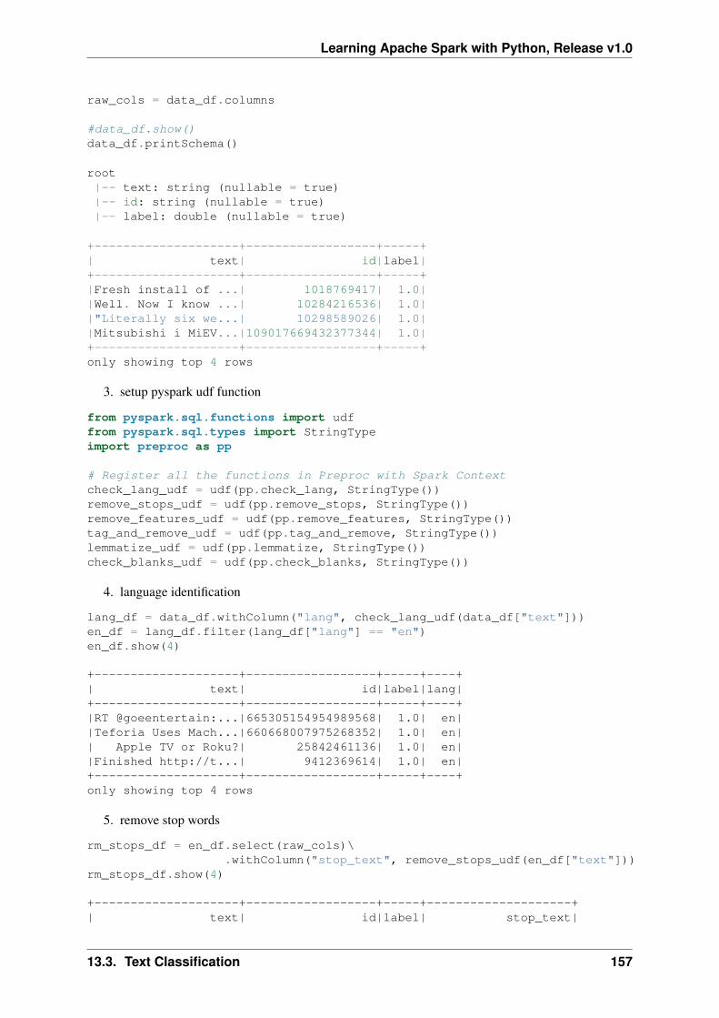
Learning Apache Spark with Python, Release v1.0
raw_cols = data_df.columns
#data_df.show()data_df.printSchema()
root|-- text: string (nullable = true)|-- id: string (nullable = true)|-- label: double (nullable = true)
+--------------------+------------------+-----+| text| id|label|+--------------------+------------------+-----+|Fresh install of ...| 1018769417| 1.0||Well. Now I know ...| 10284216536| 1.0||"Literally six we...| 10298589026| 1.0||Mitsubishi i MiEV...|109017669432377344| 1.0|+--------------------+------------------+-----+only showing top 4 rows
3. setup pyspark udf function
from pyspark.sql.functions import udffrom pyspark.sql.types import StringTypeimport preproc as pp
# Register all the functions in Preproc with Spark Contextcheck_lang_udf = udf(pp.check_lang, StringType())remove_stops_udf = udf(pp.remove_stops, StringType())remove_features_udf = udf(pp.remove_features, StringType())tag_and_remove_udf = udf(pp.tag_and_remove, StringType())lemmatize_udf = udf(pp.lemmatize, StringType())check_blanks_udf = udf(pp.check_blanks, StringType())
4. language identification
lang_df = data_df.withColumn("lang", check_lang_udf(data_df["text"]))en_df = lang_df.filter(lang_df["lang"] == "en")en_df.show(4)
+--------------------+------------------+-----+----+| text| id|label|lang|+--------------------+------------------+-----+----+|RT @goeentertain:...|665305154954989568| 1.0| en||Teforia Uses Mach...|660668007975268352| 1.0| en|| Apple TV or Roku?| 25842461136| 1.0| en||Finished http://t...| 9412369614| 1.0| en|+--------------------+------------------+-----+----+only showing top 4 rows
5. remove stop words
rm_stops_df = en_df.select(raw_cols)\.withColumn("stop_text", remove_stops_udf(en_df["text"]))
rm_stops_df.show(4)
+--------------------+------------------+-----+--------------------+| text| id|label| stop_text|
13.3. Text Classification 157
Learning Apache Spark with Python, Release v1.0
+--------------------+------------------+-----+--------------------+|RT @goeentertain:...|665305154954989568| 1.0|RT @goeentertain:...||Teforia Uses Mach...|660668007975268352| 1.0|Teforia Uses Mach...|| Apple TV or Roku?| 25842461136| 1.0| Apple TV Roku?||Finished http://t...| 9412369614| 1.0|Finished http://t...|+--------------------+------------------+-----+--------------------+only showing top 4 rows
6. remove irrelevant features
rm_features_df = rm_stops_df.select(raw_cols+["stop_text"])\.withColumn("feat_text", \remove_features_udf(rm_stops_df["stop_text"]))
rm_features_df.show(4)
+--------------------+------------------+-----+--------------------+--------------------+| text| id|label| stop_text| feat_text|+--------------------+------------------+-----+--------------------+--------------------+|RT @goeentertain:...|665305154954989568| 1.0|RT @goeentertain:...| future blase ...||Teforia Uses Mach...|660668007975268352| 1.0|Teforia Uses Mach...|teforia uses mach...|| Apple TV or Roku?| 25842461136| 1.0| Apple TV Roku?| apple roku||Finished http://t...| 9412369614| 1.0|Finished http://t...| finished|+--------------------+------------------+-----+--------------------+--------------------+only showing top 4 rows
7. tag the words
tagged_df = rm_features_df.select(raw_cols+["feat_text"]) \.withColumn("tagged_text", \tag_and_remove_udf(rm_features_df.feat_text))
tagged_df.show(4)
+--------------------+------------------+-----+--------------------+--------------------+| text| id|label| feat_text| tagged_text|+--------------------+------------------+-----+--------------------+--------------------+|RT @goeentertain:...|665305154954989568| 1.0| future blase ...| future blase vic...||Teforia Uses Mach...|660668007975268352| 1.0|teforia uses mach...| teforia uses mac...|| Apple TV or Roku?| 25842461136| 1.0| apple roku| apple roku ||Finished http://t...| 9412369614| 1.0| finished| finished |+--------------------+------------------+-----+--------------------+--------------------+only showing top 4 rows
8. lemmatization of words
lemm_df = tagged_df.select(raw_cols+["tagged_text"]) \.withColumn("lemm_text", lemmatize_udf(tagged_df["tagged_text"]))
lemm_df.show(4)
+--------------------+------------------+-----+--------------------+--------------------+| text| id|label| tagged_text| lemm_text|+--------------------+------------------+-----+--------------------+--------------------+|RT @goeentertain:...|665305154954989568| 1.0| future blase vic...|future blase vice...||Teforia Uses Mach...|660668007975268352| 1.0| teforia uses mac...|teforia use machi...|| Apple TV or Roku?| 25842461136| 1.0| apple roku | apple roku||Finished http://t...| 9412369614| 1.0| finished | finish|+--------------------+------------------+-----+--------------------+--------------------+only showing top 4 rows
158 Chapter 13. Text Mining
Learning Apache Spark with Python, Release v1.0
9. remove blank rows and drop duplicates
check_blanks_df = lemm_df.select(raw_cols+["lemm_text"])\.withColumn("is_blank", check_blanks_udf(lemm_df["lemm_text"]))
# remove blanksno_blanks_df = check_blanks_df.filter(check_blanks_df["is_blank"] == "False")
# drop duplicatesdedup_df = no_blanks_df.dropDuplicates([’text’, ’label’])
dedup_df.show(4)
+--------------------+------------------+-----+--------------------+--------+| text| id|label| lemm_text|is_blank|+--------------------+------------------+-----+--------------------+--------+|RT @goeentertain:...|665305154954989568| 1.0|future blase vice...| False||Teforia Uses Mach...|660668007975268352| 1.0|teforia use machi...| False|| Apple TV or Roku?| 25842461136| 1.0| apple roku| False||Finished http://t...| 9412369614| 1.0| finish| False|+--------------------+------------------+-----+--------------------+--------+only showing top 4 rows
10. add unieuq ID
from pyspark.sql.functions import monotonically_increasing_id# Create Unique IDdedup_df = dedup_df.withColumn("uid", monotonically_increasing_id())dedup_df.show(4)
+--------------------+------------------+-----+--------------------+--------+------------+| text| id|label| lemm_text|is_blank| uid|+--------------------+------------------+-----+--------------------+--------+------------+| dragon| 1546813742| 1.0| dragon| False| 85899345920|| hurt much| 1558492525| 1.0| hurt much| False|111669149696||seth blog word se...|383221484023709697| 1.0|seth blog word se...| False|128849018880||teforia use machi...|660668007975268352| 1.0|teforia use machi...| False|137438953472|+--------------------+------------------+-----+--------------------+--------+------------+only showing top 4 rows
11. create final dataset
data = dedup_df.select(’uid’,’id’, ’text’,’label’)data.show(4)
+------------+------------------+--------------------+-----+| uid| id| text|label|+------------+------------------+--------------------+-----+| 85899345920| 1546813742| dragon| 1.0||111669149696| 1558492525| hurt much| 1.0||128849018880|383221484023709697|seth blog word se...| 1.0||137438953472|660668007975268352|teforia use machi...| 1.0|+------------+------------------+--------------------+-----+only showing top 4 rows
12. Create taining and test sets
# Split the data into training and test sets (40% held out for testing)(trainingData, testData) = data.randomSplit([0.6, 0.4])
13.3. Text Classification 159
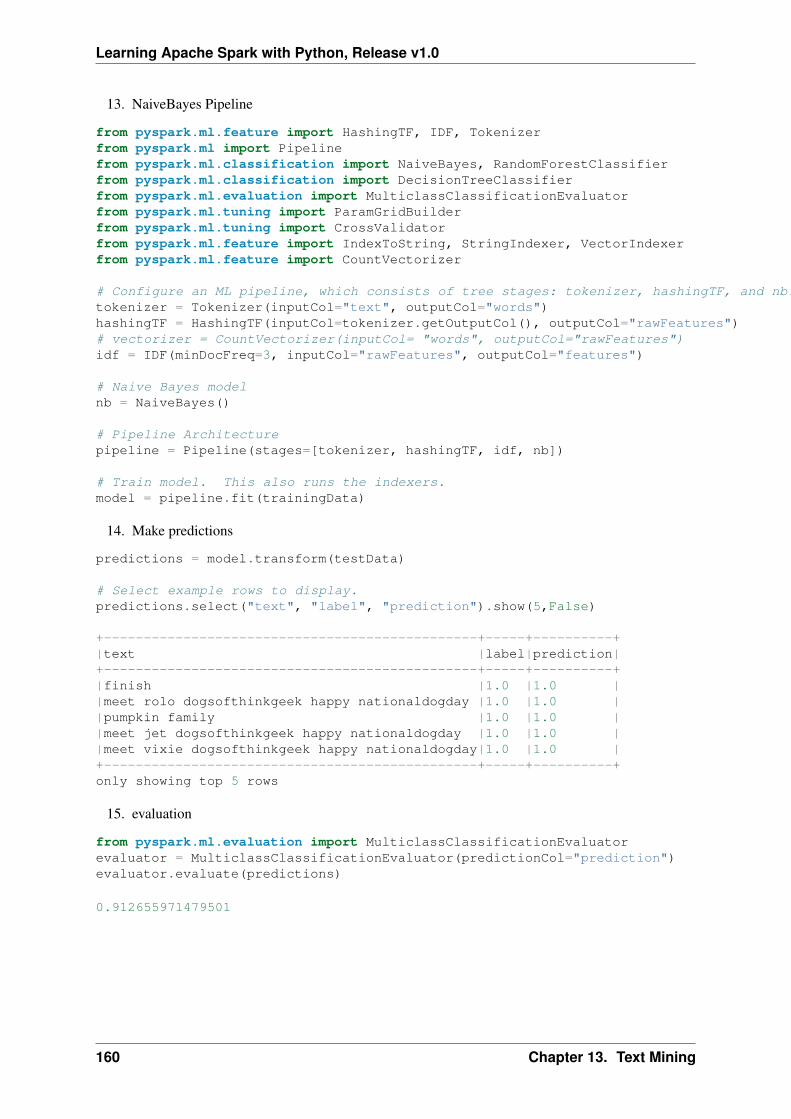
Learning Apache Spark with Python, Release v1.0
13. NaiveBayes Pipeline
from pyspark.ml.feature import HashingTF, IDF, Tokenizerfrom pyspark.ml import Pipelinefrom pyspark.ml.classification import NaiveBayes, RandomForestClassifierfrom pyspark.ml.classification import DecisionTreeClassifierfrom pyspark.ml.evaluation import MulticlassClassificationEvaluatorfrom pyspark.ml.tuning import ParamGridBuilderfrom pyspark.ml.tuning import CrossValidatorfrom pyspark.ml.feature import IndexToString, StringIndexer, VectorIndexerfrom pyspark.ml.feature import CountVectorizer
# Configure an ML pipeline, which consists of tree stages: tokenizer, hashingTF, and nb.tokenizer = Tokenizer(inputCol="text", outputCol="words")hashingTF = HashingTF(inputCol=tokenizer.getOutputCol(), outputCol="rawFeatures")# vectorizer = CountVectorizer(inputCol= "words", outputCol="rawFeatures")idf = IDF(minDocFreq=3, inputCol="rawFeatures", outputCol="features")
# Naive Bayes modelnb = NaiveBayes()
# Pipeline Architecturepipeline = Pipeline(stages=[tokenizer, hashingTF, idf, nb])
# Train model. This also runs the indexers.model = pipeline.fit(trainingData)
14. Make predictions
predictions = model.transform(testData)
# Select example rows to display.predictions.select("text", "label", "prediction").show(5,False)
+-----------------------------------------------+-----+----------+|text |label|prediction|+-----------------------------------------------+-----+----------+|finish |1.0 |1.0 ||meet rolo dogsofthinkgeek happy nationaldogday |1.0 |1.0 ||pumpkin family |1.0 |1.0 ||meet jet dogsofthinkgeek happy nationaldogday |1.0 |1.0 ||meet vixie dogsofthinkgeek happy nationaldogday|1.0 |1.0 |+-----------------------------------------------+-----+----------+only showing top 5 rows
15. evaluation
from pyspark.ml.evaluation import MulticlassClassificationEvaluatorevaluator = MulticlassClassificationEvaluator(predictionCol="prediction")evaluator.evaluate(predictions)
0.912655971479501
160 Chapter 13. Text Mining
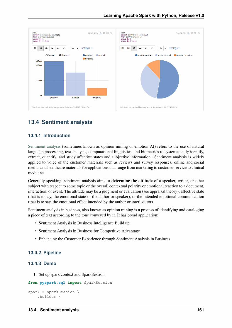
Learning Apache Spark with Python, Release v1.0
13.4 Sentiment analysis
13.4.1 Introduction
Sentiment analysis (sometimes known as opinion mining or emotion AI) refers to the use of naturallanguage processing, text analysis, computational linguistics, and biometrics to systematically identify,extract, quantify, and study affective states and subjective information. Sentiment analysis is widelyapplied to voice of the customer materials such as reviews and survey responses, online and socialmedia, and healthcare materials for applications that range from marketing to customer service to clinicalmedicine.
Generally speaking, sentiment analysis aims to determine the attitude of a speaker, writer, or othersubject with respect to some topic or the overall contextual polarity or emotional reaction to a document,interaction, or event. The attitude may be a judgment or evaluation (see appraisal theory), affective state(that is to say, the emotional state of the author or speaker), or the intended emotional communication(that is to say, the emotional effect intended by the author or interlocutor).
Sentiment analysis in business, also known as opinion mining is a process of identifying and cataloginga piece of text according to the tone conveyed by it. It has broad application:
• Sentiment Analysis in Business Intelligence Build up
• Sentiment Analysis in Business for Competitive Advantage
• Enhancing the Customer Experience through Sentiment Analysis in Business
13.4.2 Pipeline
13.4.3 Demo
1. Set up spark context and SparkSession
from pyspark.sql import SparkSession
spark = SparkSession \.builder \
13.4. Sentiment analysis 161
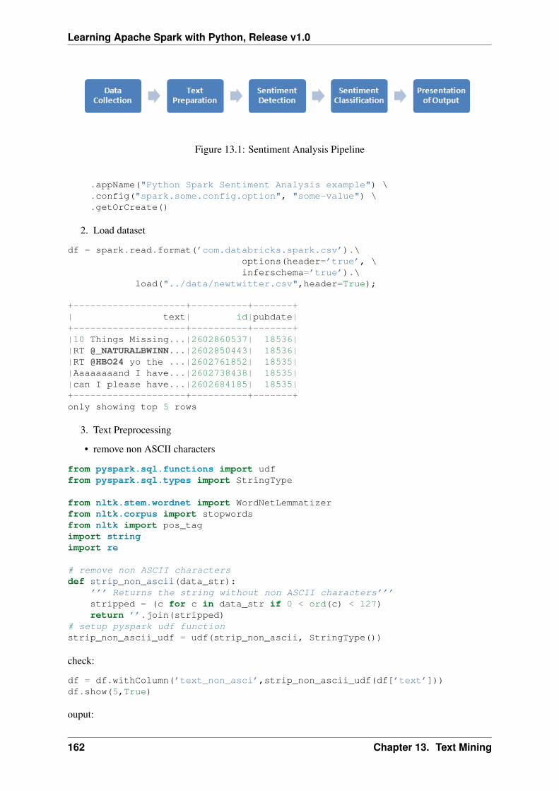
Learning Apache Spark with Python, Release v1.0
Figure 13.1: Sentiment Analysis Pipeline
.appName("Python Spark Sentiment Analysis example") \
.config("spark.some.config.option", "some-value") \
.getOrCreate()
2. Load dataset
df = spark.read.format(’com.databricks.spark.csv’).\options(header=’true’, \inferschema=’true’).\
load("../data/newtwitter.csv",header=True);
+--------------------+----------+-------+| text| id|pubdate|+--------------------+----------+-------+|10 Things Missing...|2602860537| 18536||RT @_NATURALBWINN...|2602850443| 18536||RT @HBO24 yo the ...|2602761852| 18535||Aaaaaaaand I have...|2602738438| 18535||can I please have...|2602684185| 18535|+--------------------+----------+-------+only showing top 5 rows
3. Text Preprocessing
• remove non ASCII characters
from pyspark.sql.functions import udffrom pyspark.sql.types import StringType
from nltk.stem.wordnet import WordNetLemmatizerfrom nltk.corpus import stopwordsfrom nltk import pos_tagimport stringimport re
# remove non ASCII charactersdef strip_non_ascii(data_str):
’’’ Returns the string without non ASCII characters’’’stripped = (c for c in data_str if 0 < ord(c) < 127)return ’’.join(stripped)
# setup pyspark udf functionstrip_non_ascii_udf = udf(strip_non_ascii, StringType())
check:
df = df.withColumn(’text_non_asci’,strip_non_ascii_udf(df[’text’]))df.show(5,True)
ouput:
162 Chapter 13. Text Mining

Learning Apache Spark with Python, Release v1.0
+--------------------+----------+-------+--------------------+| text| id|pubdate| text_non_asci|+--------------------+----------+-------+--------------------+|10 Things Missing...|2602860537| 18536|10 Things Missing...||RT @_NATURALBWINN...|2602850443| 18536|RT @_NATURALBWINN...||RT @HBO24 yo the ...|2602761852| 18535|RT @HBO24 yo the ...||Aaaaaaaand I have...|2602738438| 18535|Aaaaaaaand I have...||can I please have...|2602684185| 18535|can I please have...|+--------------------+----------+-------+--------------------+only showing top 5 rows
• fixed abbreviation
# fixed abbreviationdef fix_abbreviation(data_str):
data_str = data_str.lower()data_str = re.sub(r’\bthats\b’, ’that is’, data_str)data_str = re.sub(r’\bive\b’, ’i have’, data_str)data_str = re.sub(r’\bim\b’, ’i am’, data_str)data_str = re.sub(r’\bya\b’, ’yeah’, data_str)data_str = re.sub(r’\bcant\b’, ’can not’, data_str)data_str = re.sub(r’\bdont\b’, ’do not’, data_str)data_str = re.sub(r’\bwont\b’, ’will not’, data_str)data_str = re.sub(r’\bid\b’, ’i would’, data_str)data_str = re.sub(r’wtf’, ’what the fuck’, data_str)data_str = re.sub(r’\bwth\b’, ’what the hell’, data_str)data_str = re.sub(r’\br\b’, ’are’, data_str)data_str = re.sub(r’\bu\b’, ’you’, data_str)data_str = re.sub(r’\bk\b’, ’OK’, data_str)data_str = re.sub(r’\bsux\b’, ’sucks’, data_str)data_str = re.sub(r’\bno+\b’, ’no’, data_str)data_str = re.sub(r’\bcoo+\b’, ’cool’, data_str)data_str = re.sub(r’rt\b’, ’’, data_str)data_str = data_str.strip()return data_str
fix_abbreviation_udf = udf(fix_abbreviation, StringType())
check:
df = df.withColumn(’fixed_abbrev’,fix_abbreviation_udf(df[’text_non_asci’]))df.show(5,True)
ouput:
+--------------------+----------+-------+--------------------+--------------------+| text| id|pubdate| text_non_asci| fixed_abbrev|+--------------------+----------+-------+--------------------+--------------------+|10 Things Missing...|2602860537| 18536|10 Things Missing...|10 things missing...||RT @_NATURALBWINN...|2602850443| 18536|RT @_NATURALBWINN...|@_naturalbwinner ...||RT @HBO24 yo the ...|2602761852| 18535|RT @HBO24 yo the ...|@hbo24 yo the #ne...||Aaaaaaaand I have...|2602738438| 18535|Aaaaaaaand I have...|aaaaaaaand i have...||can I please have...|2602684185| 18535|can I please have...|can i please have...|+--------------------+----------+-------+--------------------+--------------------+only showing top 5 rows
• remove irrelevant features
13.4. Sentiment analysis 163
Learning Apache Spark with Python, Release v1.0
def remove_features(data_str):# compile regexurl_re = re.compile(’https?://(www.)?\w+\.\w+(/\w+)*/?’)punc_re = re.compile(’[%s]’ % re.escape(string.punctuation))num_re = re.compile(’(\\d+)’)mention_re = re.compile(’@(\w+)’)alpha_num_re = re.compile("^[a-z0-9_.]+$")# convert to lowercasedata_str = data_str.lower()# remove hyperlinksdata_str = url_re.sub(’ ’, data_str)# remove @mentionsdata_str = mention_re.sub(’ ’, data_str)# remove puncuationdata_str = punc_re.sub(’ ’, data_str)# remove numeric ’words’data_str = num_re.sub(’ ’, data_str)# remove non a-z 0-9 characters and words shorter than 1 characterslist_pos = 0cleaned_str = ’’for word in data_str.split():
if list_pos == 0:if alpha_num_re.match(word) and len(word) > 1:
cleaned_str = wordelse:
cleaned_str = ’ ’else:
if alpha_num_re.match(word) and len(word) > 1:cleaned_str = cleaned_str + ’ ’ + word
else:cleaned_str += ’ ’
list_pos += 1# remove unwanted space, *.split() will automatically split on# whitespace and discard duplicates, the " ".join() joins the# resulting list into one string.return " ".join(cleaned_str.split())
# setup pyspark udf functionremove_features_udf = udf(remove_features, StringType())
check:
df = df.withColumn(’removed’,remove_features_udf(df[’fixed_abbrev’]))df.show(5,True)
ouput:
+--------------------+----------+-------+--------------------+--------------------+--------------------+| text| id|pubdate| text_non_asci| fixed_abbrev| removed|+--------------------+----------+-------+--------------------+--------------------+--------------------+|10 Things Missing...|2602860537| 18536|10 Things Missing...|10 things missing...|things missing in...||RT @_NATURALBWINN...|2602850443| 18536|RT @_NATURALBWINN...|@_naturalbwinner ...|oh and do not lik...||RT @HBO24 yo the ...|2602761852| 18535|RT @HBO24 yo the ...|@hbo24 yo the #ne...|yo the newtwitter...||Aaaaaaaand I have...|2602738438| 18535|Aaaaaaaand I have...|aaaaaaaand i have...|aaaaaaaand have t...||can I please have...|2602684185| 18535|can I please have...|can i please have...|can please have t...|+--------------------+----------+-------+--------------------+--------------------+--------------------+only showing top 5 rows
4. Sentiment Analysis main function
164 Chapter 13. Text Mining
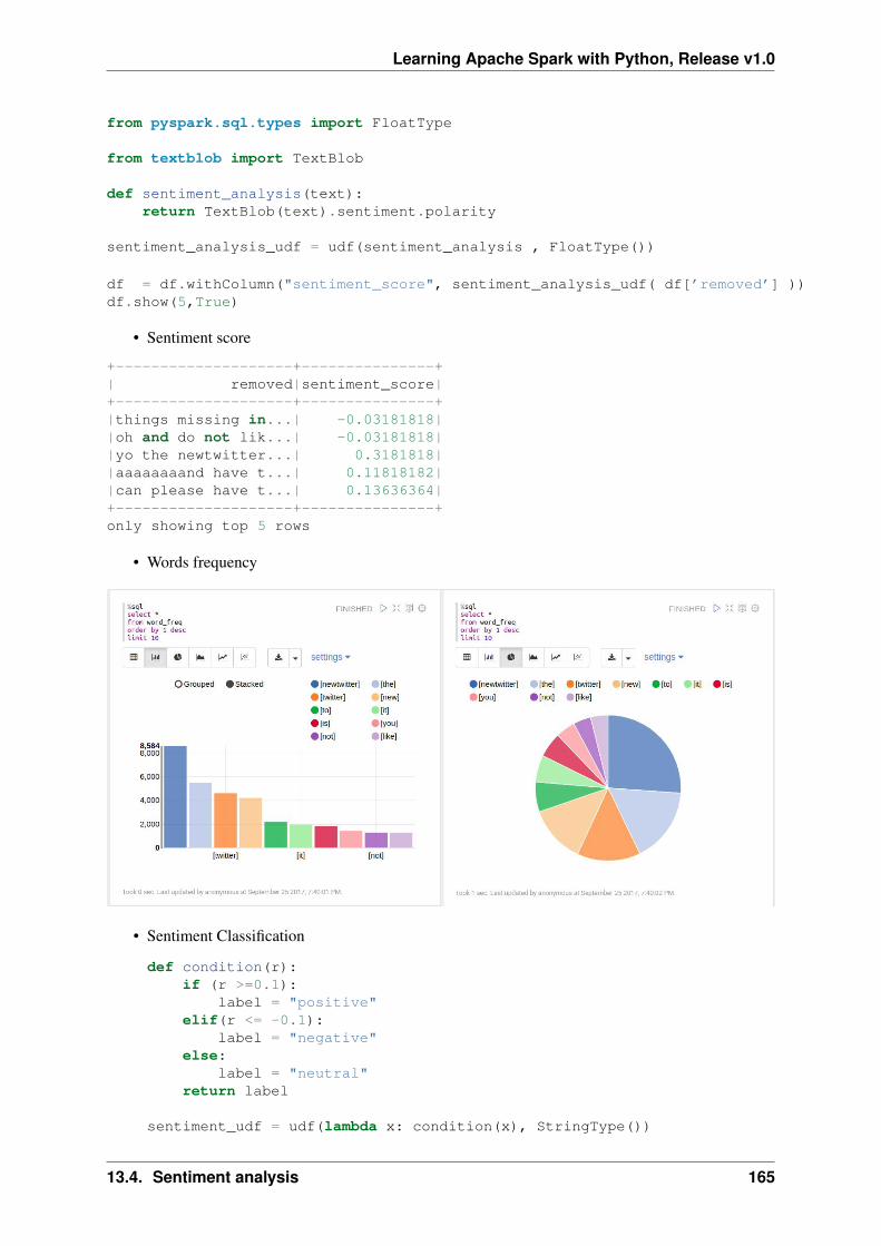
Learning Apache Spark with Python, Release v1.0
from pyspark.sql.types import FloatType
from textblob import TextBlob
def sentiment_analysis(text):return TextBlob(text).sentiment.polarity
sentiment_analysis_udf = udf(sentiment_analysis , FloatType())
df = df.withColumn("sentiment_score", sentiment_analysis_udf( df[’removed’] ))df.show(5,True)
• Sentiment score
+--------------------+---------------+| removed|sentiment_score|+--------------------+---------------+|things missing in...| -0.03181818||oh and do not lik...| -0.03181818||yo the newtwitter...| 0.3181818||aaaaaaaand have t...| 0.11818182||can please have t...| 0.13636364|+--------------------+---------------+only showing top 5 rows
• Words frequency
• Sentiment Classification
def condition(r):if (r >=0.1):
label = "positive"elif(r <= -0.1):
label = "negative"else:
label = "neutral"return label
sentiment_udf = udf(lambda x: condition(x), StringType())
13.4. Sentiment analysis 165
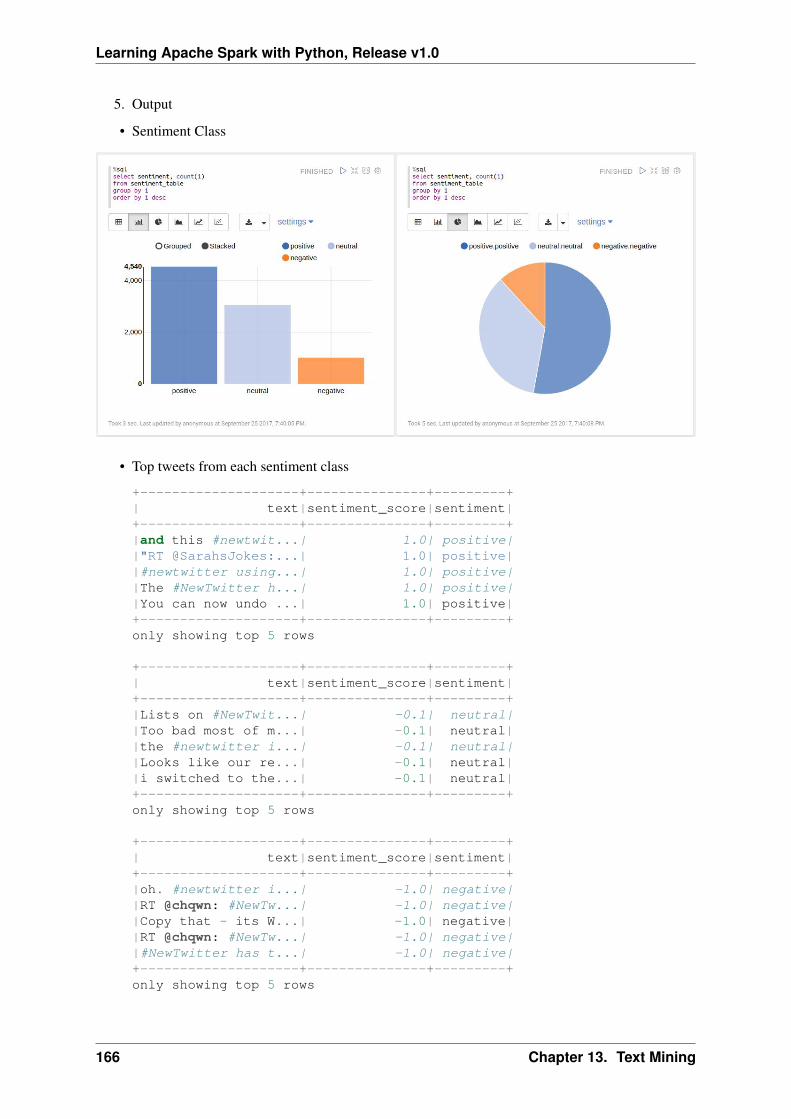
Learning Apache Spark with Python, Release v1.0
5. Output
• Sentiment Class
• Top tweets from each sentiment class
+--------------------+---------------+---------+| text|sentiment_score|sentiment|+--------------------+---------------+---------+|and this #newtwit...| 1.0| positive||"RT @SarahsJokes:...| 1.0| positive||#newtwitter using...| 1.0| positive||The #NewTwitter h...| 1.0| positive||You can now undo ...| 1.0| positive|+--------------------+---------------+---------+only showing top 5 rows
+--------------------+---------------+---------+| text|sentiment_score|sentiment|+--------------------+---------------+---------+|Lists on #NewTwit...| -0.1| neutral||Too bad most of m...| -0.1| neutral||the #newtwitter i...| -0.1| neutral||Looks like our re...| -0.1| neutral||i switched to the...| -0.1| neutral|+--------------------+---------------+---------+only showing top 5 rows
+--------------------+---------------+---------+| text|sentiment_score|sentiment|+--------------------+---------------+---------+|oh. #newtwitter i...| -1.0| negative||RT @chqwn: #NewTw...| -1.0| negative||Copy that - its W...| -1.0| negative||RT @chqwn: #NewTw...| -1.0| negative||#NewTwitter has t...| -1.0| negative|+--------------------+---------------+---------+only showing top 5 rows
166 Chapter 13. Text Mining
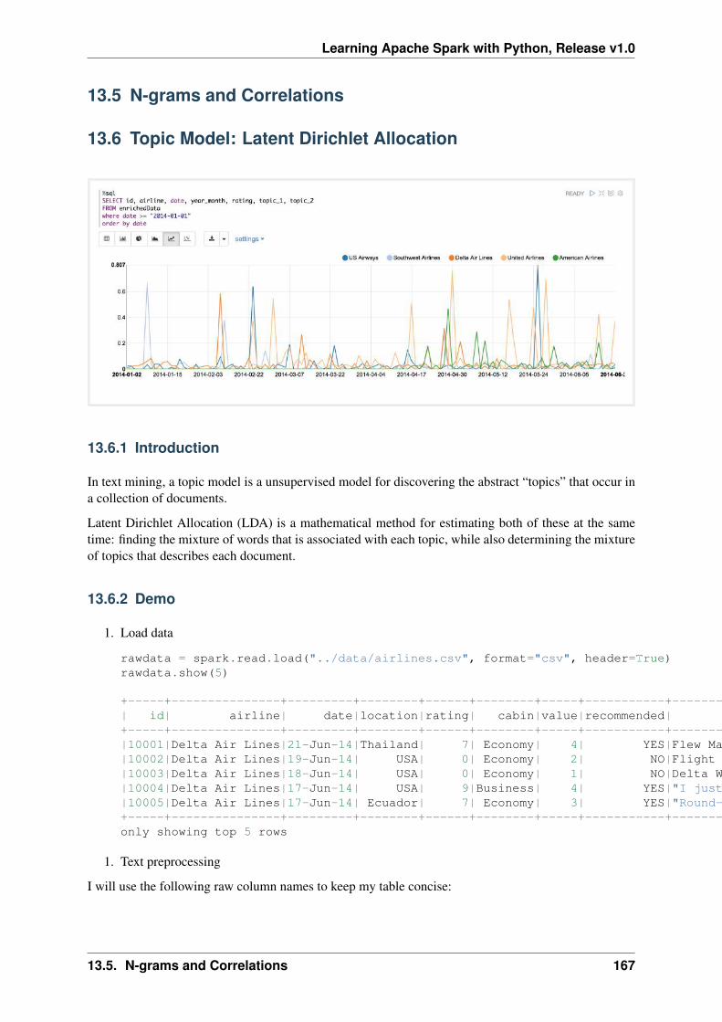
Learning Apache Spark with Python, Release v1.0
13.5 N-grams and Correlations
13.6 Topic Model: Latent Dirichlet Allocation
13.6.1 Introduction
In text mining, a topic model is a unsupervised model for discovering the abstract “topics” that occur ina collection of documents.
Latent Dirichlet Allocation (LDA) is a mathematical method for estimating both of these at the sametime: finding the mixture of words that is associated with each topic, while also determining the mixtureof topics that describes each document.
13.6.2 Demo
1. Load data
rawdata = spark.read.load("../data/airlines.csv", format="csv", header=True)rawdata.show(5)
+-----+---------------+---------+--------+------+--------+-----+-----------+--------------------+| id| airline| date|location|rating| cabin|value|recommended| review|+-----+---------------+---------+--------+------+--------+-----+-----------+--------------------+|10001|Delta Air Lines|21-Jun-14|Thailand| 7| Economy| 4| YES|Flew Mar 30 NRT t...||10002|Delta Air Lines|19-Jun-14| USA| 0| Economy| 2| NO|Flight 2463 leavi...||10003|Delta Air Lines|18-Jun-14| USA| 0| Economy| 1| NO|Delta Website fro...||10004|Delta Air Lines|17-Jun-14| USA| 9|Business| 4| YES|"I just returned ...||10005|Delta Air Lines|17-Jun-14| Ecuador| 7| Economy| 3| YES|"Round-trip fligh...|+-----+---------------+---------+--------+------+--------+-----+-----------+--------------------+only showing top 5 rows
1. Text preprocessing
I will use the following raw column names to keep my table concise:
13.5. N-grams and Correlations 167
Learning Apache Spark with Python, Release v1.0
raw_cols = rawdata.columnsraw_cols
[’id’, ’airline’, ’date’, ’location’, ’rating’, ’cabin’, ’value’, ’recommended’, ’review’]
rawdata = rawdata.dropDuplicates([’review’])
from pyspark.sql.functions import udf, colfrom pyspark.sql.types import StringType, DoubleType, DateType
from nltk.stem.wordnet import WordNetLemmatizerfrom nltk.corpus import stopwordsfrom nltk import pos_tagimport langidimport stringimport re
• remove non ASCII characters
# remove non ASCII charactersdef strip_non_ascii(data_str):
’’’ Returns the string without non ASCII characters’’’stripped = (c for c in data_str if 0 < ord(c) < 127)return ’’.join(stripped)
• check it blank line or not
# check to see if a row only contains whitespacedef check_blanks(data_str):
is_blank = str(data_str.isspace())return is_blank
• check the language (a little bit slow, I skited this step)
# check the language (only apply to english)def check_lang(data_str):
from langid.langid import LanguageIdentifier, modelidentifier = LanguageIdentifier.from_modelstring(model, norm_probs=True)predict_lang = identifier.classify(data_str)
if predict_lang[1] >= .9:language = predict_lang[0]
else:language = predict_lang[0]
return language
• fixed abbreviation
# fixed abbreviationdef fix_abbreviation(data_str):
data_str = data_str.lower()data_str = re.sub(r’\bthats\b’, ’that is’, data_str)data_str = re.sub(r’\bive\b’, ’i have’, data_str)data_str = re.sub(r’\bim\b’, ’i am’, data_str)data_str = re.sub(r’\bya\b’, ’yeah’, data_str)data_str = re.sub(r’\bcant\b’, ’can not’, data_str)data_str = re.sub(r’\bdont\b’, ’do not’, data_str)data_str = re.sub(r’\bwont\b’, ’will not’, data_str)
168 Chapter 13. Text Mining
Learning Apache Spark with Python, Release v1.0
data_str = re.sub(r’\bid\b’, ’i would’, data_str)data_str = re.sub(r’wtf’, ’what the fuck’, data_str)data_str = re.sub(r’\bwth\b’, ’what the hell’, data_str)data_str = re.sub(r’\br\b’, ’are’, data_str)data_str = re.sub(r’\bu\b’, ’you’, data_str)data_str = re.sub(r’\bk\b’, ’OK’, data_str)data_str = re.sub(r’\bsux\b’, ’sucks’, data_str)data_str = re.sub(r’\bno+\b’, ’no’, data_str)data_str = re.sub(r’\bcoo+\b’, ’cool’, data_str)data_str = re.sub(r’rt\b’, ’’, data_str)data_str = data_str.strip()return data_str
• remove irrelevant features
# remove irrelevant featuresdef remove_features(data_str):
# compile regexurl_re = re.compile(’https?://(www.)?\w+\.\w+(/\w+)*/?’)punc_re = re.compile(’[%s]’ % re.escape(string.punctuation))num_re = re.compile(’(\\d+)’)mention_re = re.compile(’@(\w+)’)alpha_num_re = re.compile("^[a-z0-9_.]+$")# convert to lowercasedata_str = data_str.lower()# remove hyperlinksdata_str = url_re.sub(’ ’, data_str)# remove @mentionsdata_str = mention_re.sub(’ ’, data_str)# remove puncuationdata_str = punc_re.sub(’ ’, data_str)# remove numeric ’words’data_str = num_re.sub(’ ’, data_str)# remove non a-z 0-9 characters and words shorter than 1 characterslist_pos = 0cleaned_str = ’’for word in data_str.split():
if list_pos == 0:if alpha_num_re.match(word) and len(word) > 1:
cleaned_str = wordelse:
cleaned_str = ’ ’else:
if alpha_num_re.match(word) and len(word) > 1:cleaned_str = cleaned_str + ’ ’ + word
else:cleaned_str += ’ ’
list_pos += 1# remove unwanted space, *.split() will automatically split on# whitespace and discard duplicates, the " ".join() joins the# resulting list into one string.return " ".join(cleaned_str.split())
• removes stop words
# removes stop wordsdef remove_stops(data_str):
# expects a string
13.6. Topic Model: Latent Dirichlet Allocation 169
Learning Apache Spark with Python, Release v1.0
stops = set(stopwords.words("english"))list_pos = 0cleaned_str = ’’text = data_str.split()for word in text:
if word not in stops:# rebuild cleaned_strif list_pos == 0:
cleaned_str = wordelse:
cleaned_str = cleaned_str + ’ ’ + wordlist_pos += 1
return cleaned_str
• Part-of-Speech Tagging
# Part-of-Speech Taggingdef tag_and_remove(data_str):
cleaned_str = ’ ’# noun tagsnn_tags = [’NN’, ’NNP’, ’NNP’, ’NNPS’, ’NNS’]# adjectivesjj_tags = [’JJ’, ’JJR’, ’JJS’]# verbsvb_tags = [’VB’, ’VBD’, ’VBG’, ’VBN’, ’VBP’, ’VBZ’]nltk_tags = nn_tags + jj_tags + vb_tags
# break string into ’words’text = data_str.split()
# tag the text and keep only those with the right tagstagged_text = pos_tag(text)for tagged_word in tagged_text:
if tagged_word[1] in nltk_tags:cleaned_str += tagged_word[0] + ’ ’
return cleaned_str
• lemmatization
# lemmatizationdef lemmatize(data_str):
# expects a stringlist_pos = 0cleaned_str = ’’lmtzr = WordNetLemmatizer()text = data_str.split()tagged_words = pos_tag(text)for word in tagged_words:
if ’v’ in word[1].lower():lemma = lmtzr.lemmatize(word[0], pos=’v’)
else:lemma = lmtzr.lemmatize(word[0], pos=’n’)
if list_pos == 0:cleaned_str = lemma
else:cleaned_str = cleaned_str + ’ ’ + lemma
list_pos += 1
170 Chapter 13. Text Mining
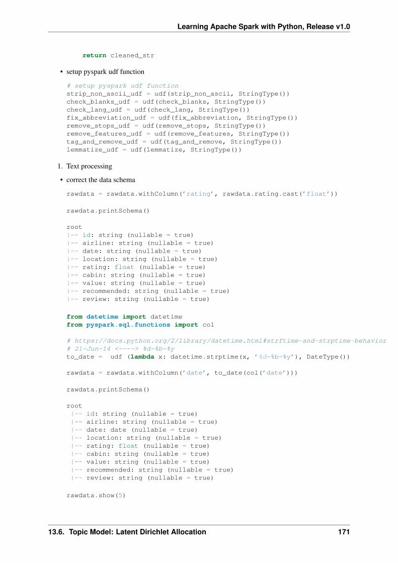
Learning Apache Spark with Python, Release v1.0
return cleaned_str
• setup pyspark udf function
# setup pyspark udf functionstrip_non_ascii_udf = udf(strip_non_ascii, StringType())check_blanks_udf = udf(check_blanks, StringType())check_lang_udf = udf(check_lang, StringType())fix_abbreviation_udf = udf(fix_abbreviation, StringType())remove_stops_udf = udf(remove_stops, StringType())remove_features_udf = udf(remove_features, StringType())tag_and_remove_udf = udf(tag_and_remove, StringType())lemmatize_udf = udf(lemmatize, StringType())
1. Text processing
• correct the data schema
rawdata = rawdata.withColumn(’rating’, rawdata.rating.cast(’float’))
rawdata.printSchema()
root|-- id: string (nullable = true)|-- airline: string (nullable = true)|-- date: string (nullable = true)|-- location: string (nullable = true)|-- rating: float (nullable = true)|-- cabin: string (nullable = true)|-- value: string (nullable = true)|-- recommended: string (nullable = true)|-- review: string (nullable = true)
from datetime import datetimefrom pyspark.sql.functions import col
# https://docs.python.org/2/library/datetime.html#strftime-and-strptime-behavior# 21-Jun-14 <----> %d-%b-%yto_date = udf (lambda x: datetime.strptime(x, ’%d-%b-%y’), DateType())
rawdata = rawdata.withColumn(’date’, to_date(col(’date’)))
rawdata.printSchema()
root|-- id: string (nullable = true)|-- airline: string (nullable = true)|-- date: date (nullable = true)|-- location: string (nullable = true)|-- rating: float (nullable = true)|-- cabin: string (nullable = true)|-- value: string (nullable = true)|-- recommended: string (nullable = true)|-- review: string (nullable = true)
rawdata.show(5)
13.6. Topic Model: Latent Dirichlet Allocation 171

Learning Apache Spark with Python, Release v1.0
+-----+------------------+----------+--------+------+--------+-----+-----------+--------------------+| id| airline| date|location|rating| cabin|value|recommended| review|+-----+------------------+----------+--------+------+--------+-----+-----------+--------------------+|10551|Southwest Airlines|2013-11-06| USA| 1.0|Business| 2| NO|Flight 3246 from ...||10298| US Airways|2014-03-31| UK| 1.0|Business| 0| NO|Flight from Manch...||10564|Southwest Airlines|2013-09-06| USA| 10.0| Economy| 5| YES|I’m Executive Pla...||10134| Delta Air Lines|2013-12-10| USA| 8.0| Economy| 4| YES|MSP-JFK-MXP and r...||10912| United Airlines|2014-04-07| USA| 3.0| Economy| 1| NO|Worst airline I h...|+-----+------------------+----------+--------+------+--------+-----+-----------+--------------------+only showing top 5 rows
rawdata = rawdata.withColumn(’non_asci’, strip_non_ascii_udf(rawdata[’review’]))
+-----+------------------+----------+--------+------+--------+-----+-----------+--------------------+--------------------+| id| airline| date|location|rating| cabin|value|recommended| review| non_asci|+-----+------------------+----------+--------+------+--------+-----+-----------+--------------------+--------------------+|10551|Southwest Airlines|2013-11-06| USA| 1.0|Business| 2| NO|Flight 3246 from ...|Flight 3246 from ...||10298| US Airways|2014-03-31| UK| 1.0|Business| 0| NO|Flight from Manch...|Flight from Manch...||10564|Southwest Airlines|2013-09-06| USA| 10.0| Economy| 5| YES|I’m Executive Pla...|I’m Executive Pla...||10134| Delta Air Lines|2013-12-10| USA| 8.0| Economy| 4| YES|MSP-JFK-MXP and r...|MSP-JFK-MXP and r...||10912| United Airlines|2014-04-07| USA| 3.0| Economy| 1| NO|Worst airline I h...|Worst airline I h...|+-----+------------------+----------+--------+------+--------+-----+-----------+--------------------+--------------------+only showing top 5 rows
rawdata = rawdata.select(raw_cols+[’non_asci’])\.withColumn(’fixed_abbrev’,fix_abbreviation_udf(rawdata[’non_asci’]))
+-----+------------------+----------+--------+------+--------+-----+-----------+--------------------+--------------------+--------------------+| id| airline| date|location|rating| cabin|value|recommended| review| non_asci| fixed_abbrev|+-----+------------------+----------+--------+------+--------+-----+-----------+--------------------+--------------------+--------------------+|10551|Southwest Airlines|2013-11-06| USA| 1.0|Business| 2| NO|Flight 3246 from ...|Flight 3246 from ...|flight 3246 from ...||10298| US Airways|2014-03-31| UK| 1.0|Business| 0| NO|Flight from Manch...|Flight from Manch...|flight from manch...||10564|Southwest Airlines|2013-09-06| USA| 10.0| Economy| 5| YES|I’m Executive Pla...|I’m Executive Pla...|i’m executive pla...||10134| Delta Air Lines|2013-12-10| USA| 8.0| Economy| 4| YES|MSP-JFK-MXP and r...|MSP-JFK-MXP and r...|msp-jfk-mxp and r...||10912| United Airlines|2014-04-07| USA| 3.0| Economy| 1| NO|Worst airline I h...|Worst airline I h...|worst airline i h...|+-----+------------------+----------+--------+------+--------+-----+-----------+--------------------+--------------------+--------------------+only showing top 5 rows
rawdata = rawdata.select(raw_cols+[’fixed_abbrev’])\.withColumn(’stop_text’,remove_stops_udf(rawdata[’fixed_abbrev’]))
+-----+------------------+----------+--------+------+--------+-----+-----------+--------------------+--------------------+--------------------+| id| airline| date|location|rating| cabin|value|recommended| review| fixed_abbrev| stop_text|+-----+------------------+----------+--------+------+--------+-----+-----------+--------------------+--------------------+--------------------+|10551|Southwest Airlines|2013-11-06| USA| 1.0|Business| 2| NO|Flight 3246 from ...|flight 3246 from ...|flight 3246 chica...||10298| US Airways|2014-03-31| UK| 1.0|Business| 0| NO|Flight from Manch...|flight from manch...|flight manchester...||10564|Southwest Airlines|2013-09-06| USA| 10.0| Economy| 5| YES|I’m Executive Pla...|i’m executive pla...|i’m executive pla...||10134| Delta Air Lines|2013-12-10| USA| 8.0| Economy| 4| YES|MSP-JFK-MXP and r...|msp-jfk-mxp and r...|msp-jfk-mxp retur...||10912| United Airlines|2014-04-07| USA| 3.0| Economy| 1| NO|Worst airline I h...|worst airline i h...|worst airline eve...|+-----+------------------+----------+--------+------+--------+-----+-----------+--------------------+--------------------+--------------------+only showing top 5 rows
rawdata = rawdata.select(raw_cols+[’stop_text’])\.withColumn(’feat_text’,remove_features_udf(rawdata[’stop_text’]))
+-----+------------------+----------+--------+------+--------+-----+-----------+--------------------+--------------------+--------------------+
172 Chapter 13. Text Mining
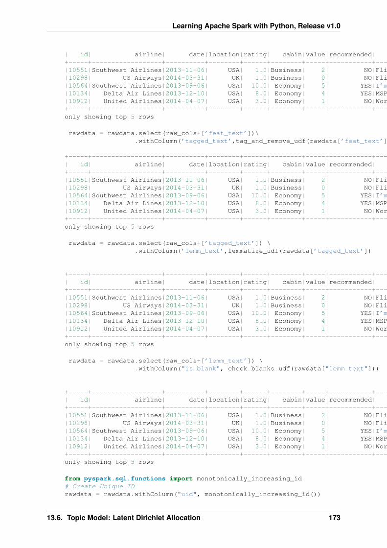
Learning Apache Spark with Python, Release v1.0
| id| airline| date|location|rating| cabin|value|recommended| review| stop_text| feat_text|+-----+------------------+----------+--------+------+--------+-----+-----------+--------------------+--------------------+--------------------+|10551|Southwest Airlines|2013-11-06| USA| 1.0|Business| 2| NO|Flight 3246 from ...|flight 3246 chica...|flight chicago mi...||10298| US Airways|2014-03-31| UK| 1.0|Business| 0| NO|Flight from Manch...|flight manchester...|flight manchester...||10564|Southwest Airlines|2013-09-06| USA| 10.0| Economy| 5| YES|I’m Executive Pla...|i’m executive pla...|executive platinu...||10134| Delta Air Lines|2013-12-10| USA| 8.0| Economy| 4| YES|MSP-JFK-MXP and r...|msp-jfk-mxp retur...|msp jfk mxp retur...||10912| United Airlines|2014-04-07| USA| 3.0| Economy| 1| NO|Worst airline I h...|worst airline eve...|worst airline eve...|+-----+------------------+----------+--------+------+--------+-----+-----------+--------------------+--------------------+--------------------+only showing top 5 rows
rawdata = rawdata.select(raw_cols+[’feat_text’])\.withColumn(’tagged_text’,tag_and_remove_udf(rawdata[’feat_text’]))
+-----+------------------+----------+--------+------+--------+-----+-----------+--------------------+--------------------+--------------------+| id| airline| date|location|rating| cabin|value|recommended| review| feat_text| tagged_text|+-----+------------------+----------+--------+------+--------+-----+-----------+--------------------+--------------------+--------------------+|10551|Southwest Airlines|2013-11-06| USA| 1.0|Business| 2| NO|Flight 3246 from ...|flight chicago mi...| flight chicago m...||10298| US Airways|2014-03-31| UK| 1.0|Business| 0| NO|Flight from Manch...|flight manchester...| flight mancheste...||10564|Southwest Airlines|2013-09-06| USA| 10.0| Economy| 5| YES|I’m Executive Pla...|executive platinu...| executive platin...||10134| Delta Air Lines|2013-12-10| USA| 8.0| Economy| 4| YES|MSP-JFK-MXP and r...|msp jfk mxp retur...| msp jfk mxp retu...||10912| United Airlines|2014-04-07| USA| 3.0| Economy| 1| NO|Worst airline I h...|worst airline eve...| worst airline ua...|+-----+------------------+----------+--------+------+--------+-----+-----------+--------------------+--------------------+--------------------+only showing top 5 rows
rawdata = rawdata.select(raw_cols+[’tagged_text’]) \.withColumn(’lemm_text’,lemmatize_udf(rawdata[’tagged_text’])
+-----+------------------+----------+--------+------+--------+-----+-----------+--------------------+--------------------+--------------------+| id| airline| date|location|rating| cabin|value|recommended| review| tagged_text| lemm_text|+-----+------------------+----------+--------+------+--------+-----+-----------+--------------------+--------------------+--------------------+|10551|Southwest Airlines|2013-11-06| USA| 1.0|Business| 2| NO|Flight 3246 from ...| flight chicago m...|flight chicago mi...||10298| US Airways|2014-03-31| UK| 1.0|Business| 0| NO|Flight from Manch...| flight mancheste...|flight manchester...||10564|Southwest Airlines|2013-09-06| USA| 10.0| Economy| 5| YES|I’m Executive Pla...| executive platin...|executive platinu...||10134| Delta Air Lines|2013-12-10| USA| 8.0| Economy| 4| YES|MSP-JFK-MXP and r...| msp jfk mxp retu...|msp jfk mxp retur...||10912| United Airlines|2014-04-07| USA| 3.0| Economy| 1| NO|Worst airline I h...| worst airline ua...|worst airline ual...|+-----+------------------+----------+--------+------+--------+-----+-----------+--------------------+--------------------+--------------------+only showing top 5 rows
rawdata = rawdata.select(raw_cols+[’lemm_text’]) \.withColumn("is_blank", check_blanks_udf(rawdata["lemm_text"]))
+-----+------------------+----------+--------+------+--------+-----+-----------+--------------------+--------------------+--------+| id| airline| date|location|rating| cabin|value|recommended| review| lemm_text|is_blank|+-----+------------------+----------+--------+------+--------+-----+-----------+--------------------+--------------------+--------+|10551|Southwest Airlines|2013-11-06| USA| 1.0|Business| 2| NO|Flight 3246 from ...|flight chicago mi...| False||10298| US Airways|2014-03-31| UK| 1.0|Business| 0| NO|Flight from Manch...|flight manchester...| False||10564|Southwest Airlines|2013-09-06| USA| 10.0| Economy| 5| YES|I’m Executive Pla...|executive platinu...| False||10134| Delta Air Lines|2013-12-10| USA| 8.0| Economy| 4| YES|MSP-JFK-MXP and r...|msp jfk mxp retur...| False||10912| United Airlines|2014-04-07| USA| 3.0| Economy| 1| NO|Worst airline I h...|worst airline ual...| False|+-----+------------------+----------+--------+------+--------+-----+-----------+--------------------+--------------------+--------+only showing top 5 rows
from pyspark.sql.functions import monotonically_increasing_id# Create Unique IDrawdata = rawdata.withColumn("uid", monotonically_increasing_id())
13.6. Topic Model: Latent Dirichlet Allocation 173
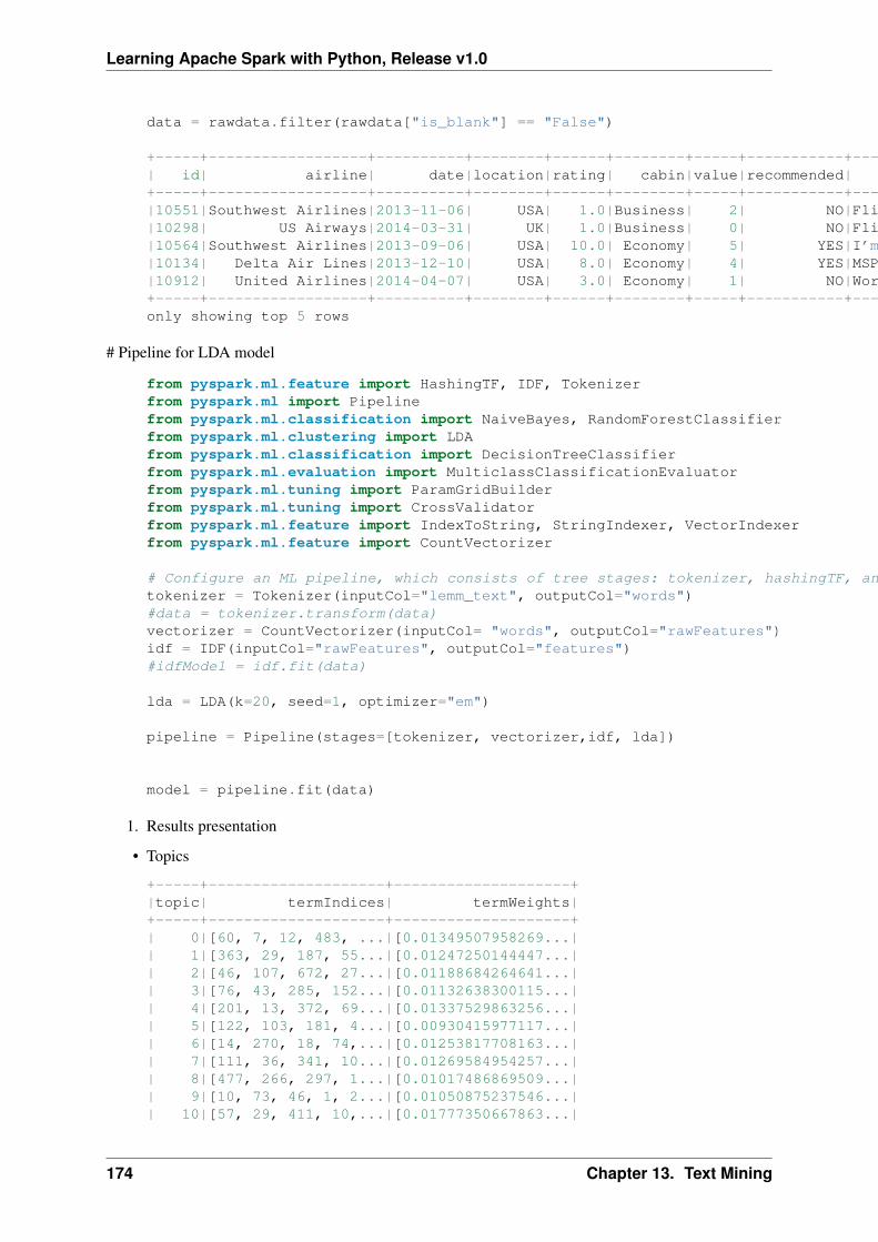
Learning Apache Spark with Python, Release v1.0
data = rawdata.filter(rawdata["is_blank"] == "False")
+-----+------------------+----------+--------+------+--------+-----+-----------+--------------------+--------------------+--------+---+| id| airline| date|location|rating| cabin|value|recommended| review| lemm_text|is_blank|uid|+-----+------------------+----------+--------+------+--------+-----+-----------+--------------------+--------------------+--------+---+|10551|Southwest Airlines|2013-11-06| USA| 1.0|Business| 2| NO|Flight 3246 from ...|flight chicago mi...| False| 0||10298| US Airways|2014-03-31| UK| 1.0|Business| 0| NO|Flight from Manch...|flight manchester...| False| 1||10564|Southwest Airlines|2013-09-06| USA| 10.0| Economy| 5| YES|I’m Executive Pla...|executive platinu...| False| 2||10134| Delta Air Lines|2013-12-10| USA| 8.0| Economy| 4| YES|MSP-JFK-MXP and r...|msp jfk mxp retur...| False| 3||10912| United Airlines|2014-04-07| USA| 3.0| Economy| 1| NO|Worst airline I h...|worst airline ual...| False| 4|+-----+------------------+----------+--------+------+--------+-----+-----------+--------------------+--------------------+--------+---+only showing top 5 rows
# Pipeline for LDA model
from pyspark.ml.feature import HashingTF, IDF, Tokenizerfrom pyspark.ml import Pipelinefrom pyspark.ml.classification import NaiveBayes, RandomForestClassifierfrom pyspark.ml.clustering import LDAfrom pyspark.ml.classification import DecisionTreeClassifierfrom pyspark.ml.evaluation import MulticlassClassificationEvaluatorfrom pyspark.ml.tuning import ParamGridBuilderfrom pyspark.ml.tuning import CrossValidatorfrom pyspark.ml.feature import IndexToString, StringIndexer, VectorIndexerfrom pyspark.ml.feature import CountVectorizer
# Configure an ML pipeline, which consists of tree stages: tokenizer, hashingTF, and nb.tokenizer = Tokenizer(inputCol="lemm_text", outputCol="words")#data = tokenizer.transform(data)vectorizer = CountVectorizer(inputCol= "words", outputCol="rawFeatures")idf = IDF(inputCol="rawFeatures", outputCol="features")#idfModel = idf.fit(data)
lda = LDA(k=20, seed=1, optimizer="em")
pipeline = Pipeline(stages=[tokenizer, vectorizer,idf, lda])
model = pipeline.fit(data)
1. Results presentation
• Topics
+-----+--------------------+--------------------+|topic| termIndices| termWeights|+-----+--------------------+--------------------+| 0|[60, 7, 12, 483, ...|[0.01349507958269...|| 1|[363, 29, 187, 55...|[0.01247250144447...|| 2|[46, 107, 672, 27...|[0.01188684264641...|| 3|[76, 43, 285, 152...|[0.01132638300115...|| 4|[201, 13, 372, 69...|[0.01337529863256...|| 5|[122, 103, 181, 4...|[0.00930415977117...|| 6|[14, 270, 18, 74,...|[0.01253817708163...|| 7|[111, 36, 341, 10...|[0.01269584954257...|| 8|[477, 266, 297, 1...|[0.01017486869509...|| 9|[10, 73, 46, 1, 2...|[0.01050875237546...|| 10|[57, 29, 411, 10,...|[0.01777350667863...|
174 Chapter 13. Text Mining
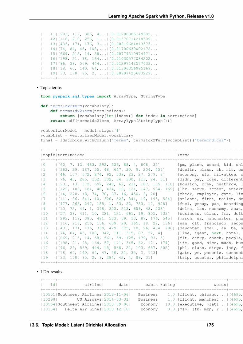
Learning Apache Spark with Python, Release v1.0
| 11|[293, 119, 385, 4...|[0.01280305149305...|| 12|[116, 218, 256, 1...|[0.01570714218509...|| 13|[433, 171, 176, 3...|[0.00819684813575...|| 14|[74, 84, 45, 108,...|[0.01700630002172...|| 15|[669, 215, 14, 58...|[0.00779310974971...|| 16|[198, 21, 98, 164...|[0.01030577084202...|| 17|[96, 29, 569, 444...|[0.01297142577633...|| 18|[18, 60, 140, 64,...|[0.01306356985169...|| 19|[33, 178, 95, 2, ...|[0.00907425683229...|+-----+--------------------+--------------------+
• Topic terms
from pyspark.sql.types import ArrayType, StringType
def termsIdx2Term(vocabulary):def termsIdx2Term(termIndices):
return [vocabulary[int(index)] for index in termIndices]return udf(termsIdx2Term, ArrayType(StringType()))
vectorizerModel = model.stages[1]vocabList = vectorizerModel.vocabularyfinal = ldatopics.withColumn("Terms", termsIdx2Term(vocabList)("termIndices"))
+-----+------------------------------------------------+-------------------------------------------------------------------------------------+|topic|termIndices |Terms |+-----+------------------------------------------------+-------------------------------------------------------------------------------------+|0 |[60, 7, 12, 483, 292, 326, 88, 4, 808, 32] |[pm, plane, board, kid, online, lga, schedule, get, memphis, arrive] ||1 |[363, 29, 187, 55, 48, 647, 30, 9, 204, 457] |[dublin, class, th, sit, entertainment, express, say, delay, dl, son] ||2 |[46, 107, 672, 274, 92, 539, 23, 27, 279, 8] |[economy, sfo, milwaukee, decent, comfortable, iad, return, united, average, airline]||3 |[76, 43, 285, 152, 102, 34, 300, 113, 24, 31] |[didn, pay, lose, different, extra, bag, mile, baggage, leave, day] ||4 |[201, 13, 372, 692, 248, 62, 211, 187, 105, 110]|[houston, crew, heathrow, louisville, london, great, denver, th, land, jfk] ||5 |[122, 103, 181, 48, 434, 10, 121, 147, 934, 169]|[lhr, serve, screen, entertainment, ny, delta, excellent, atl, sin, newark] ||6 |[14, 270, 18, 74, 70, 37, 16, 450, 3, 20] |[check, employee, gate, line, change, wait, take, fll, time, tell] ||7 |[111, 36, 341, 10, 320, 528, 844, 19, 195, 524] |[atlanta, first, toilet, delta, washington, card, global, staff, route, amsterdam] ||8 |[477, 266, 297, 185, 1, 33, 22, 783, 17, 908] |[fuel, group, pas, boarding, seat, trip, minute, orleans, make, select] ||9 |[10, 73, 46, 1, 248, 302, 213, 659, 48, 228] |[delta, lax, economy, seat, london, detroit, comfo, weren, entertainment, wife] ||10 |[57, 29, 411, 10, 221, 121, 661, 19, 805, 733] |[business, class, fra, delta, lounge, excellent, syd, staff, nov, mexico] ||11 |[293, 119, 385, 481, 503, 69, 13, 87, 176, 545] |[march, ua, manchester, phx, envoy, drink, crew, american, aa, canada] ||12 |[116, 218, 256, 156, 639, 20, 365, 18, 22, 136] |[san, clt, francisco, second, text, tell, captain, gate, minute, available] ||13 |[433, 171, 176, 339, 429, 575, 10, 26, 474, 796]|[daughter, small, aa, ba, segment, proceed, delta, passenger, size, similar] ||14 |[74, 84, 45, 108, 342, 111, 315, 87, 52, 4] |[line, agent, next, hotel, standby, atlanta, dallas, american, book, get] ||15 |[669, 215, 14, 58, 561, 59, 125, 179, 93, 5] |[fit, carry, check, people, bathroom, ask, thing, row, don, fly] ||16 |[198, 21, 98, 164, 57, 141, 345, 62, 121, 174] |[ife, good, nice, much, business, lot, dfw, great, excellent, carrier] ||17 |[96, 29, 569, 444, 15, 568, 21, 103, 657, 505] |[phl, class, diego, lady, food, wheelchair, good, serve, miami, mia] ||18 |[18, 60, 140, 64, 47, 40, 31, 35, 2, 123] |[gate, pm, phoenix, connection, cancel, connect, day, airpo, hour, charlotte] ||19 |[33, 178, 95, 2, 9, 284, 42, 4, 89, 31] |[trip, counter, philadelphia, hour, delay, stay, way, get, southwest, day] |+-----+------------------------------------------------+-------------------------------------------------------------------------------------+
• LDA results
+-----+------------------+----------+-----------+------+--------------------+--------------------+--------------------+| id| airline| date| cabin|rating| words| features| topicDistribution|+-----+------------------+----------+-----------+------+--------------------+--------------------+--------------------+|10551|Southwest Airlines|2013-11-06| Business| 1.0|[flight, chicago,...|(4695,[0,2,3,6,11...|[0.03640342580508...||10298| US Airways|2014-03-31| Business| 1.0|[flight, manchest...|(4695,[0,1,2,6,7,...|[0.01381306271470...||10564|Southwest Airlines|2013-09-06| Economy| 10.0|[executive, plati...|(4695,[0,1,6,7,11...|[0.05063554352934...||10134| Delta Air Lines|2013-12-10| Economy| 8.0|[msp, jfk, mxp, r...|(4695,[0,1,3,10,1...|[0.01494708959842...|
13.6. Topic Model: Latent Dirichlet Allocation 175
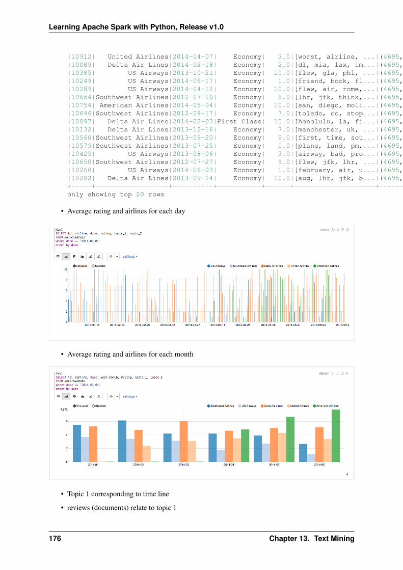
Learning Apache Spark with Python, Release v1.0
|10912| United Airlines|2014-04-07| Economy| 3.0|[worst, airline, ...|(4695,[0,1,7,8,13...|[0.04421751181232...||10089| Delta Air Lines|2014-02-18| Economy| 2.0|[dl, mia, lax, im...|(4695,[2,4,5,7,8,...|[0.02158861273876...||10385| US Airways|2013-10-21| Economy| 10.0|[flew, gla, phl, ...|(4695,[0,1,3,5,14...|[0.03343845991816...||10249| US Airways|2014-06-17| Economy| 1.0|[friend, book, fl...|(4695,[0,2,3,4,5,...|[0.02362432562165...||10289| US Airways|2014-04-12| Economy| 10.0|[flew, air, rome,...|(4695,[0,1,5,8,13...|[0.01664012816210...||10654|Southwest Airlines|2012-07-10| Economy| 8.0|[lhr, jfk, think,...|(4695,[0,4,5,6,8,...|[0.01526072330297...||10754| American Airlines|2014-05-04| Economy| 10.0|[san, diego, moli...|(4695,[0,2,8,15,2...|[0.03571177612496...||10646|Southwest Airlines|2012-08-17| Economy| 7.0|[toledo, co, stop...|(4695,[0,2,3,4,7,...|[0.02394775146271...||10097| Delta Air Lines|2014-02-03|First Class| 10.0|[honolulu, la, fi...|(4695,[0,4,6,7,13...|[0.02008375619661...||10132| Delta Air Lines|2013-12-16| Economy| 7.0|[manchester, uk, ...|(4695,[0,1,2,3,5,...|[0.01463126146601...||10560|Southwest Airlines|2013-09-20| Economy| 9.0|[first, time, sou...|(4695,[0,3,7,8,9,...|[0.04934836409896...||10579|Southwest Airlines|2013-07-25| Economy| 0.0|[plane, land, pm,...|(4695,[2,3,4,5,7,...|[0.06106959241722...||10425| US Airways|2013-08-06| Economy| 3.0|[airway, bad, pro...|(4695,[2,3,4,7,8,...|[0.01770471771322...||10650|Southwest Airlines|2012-07-27| Economy| 9.0|[flew, jfk, lhr, ...|(4695,[0,1,6,13,1...|[0.02676226245086...||10260| US Airways|2014-06-03| Economy| 1.0|[february, air, u...|(4695,[0,2,4,17,2...|[0.02887390875079...||10202| Delta Air Lines|2013-09-14| Economy| 10.0|[aug, lhr, jfk, b...|(4695,[1,2,4,7,10...|[0.02377704988307...|+-----+------------------+----------+-----------+------+--------------------+--------------------+--------------------+only showing top 20 rows
• Average rating and airlines for each day
• Average rating and airlines for each month
• Topic 1 corresponding to time line
• reviews (documents) relate to topic 1
176 Chapter 13. Text Mining
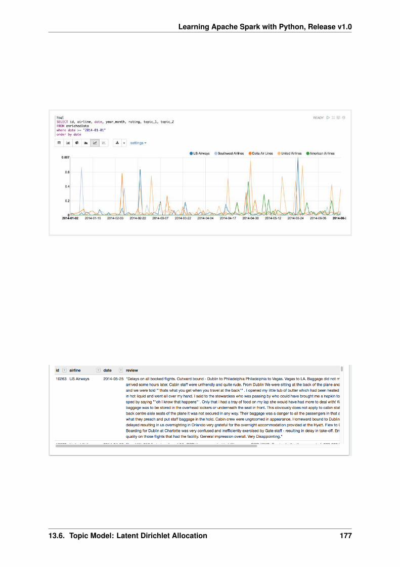
Learning Apache Spark with Python, Release v1.0
13.6. Topic Model: Latent Dirichlet Allocation 177
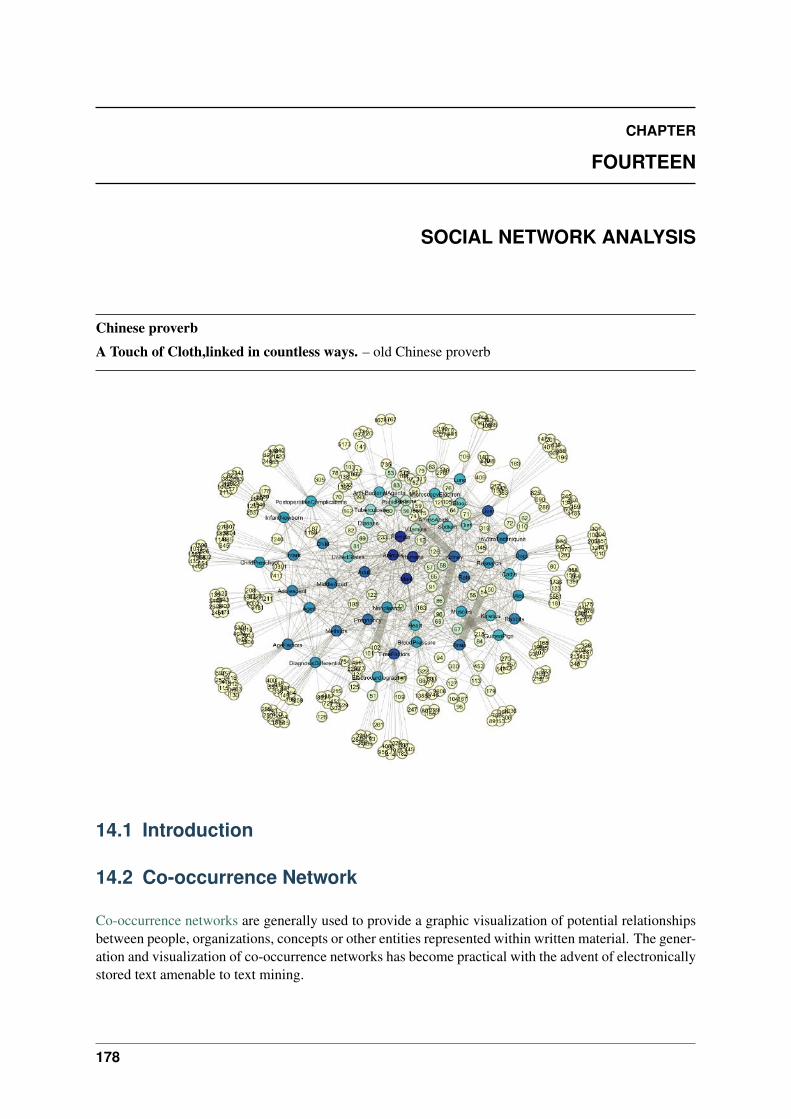
CHAPTER
FOURTEEN
SOCIAL NETWORK ANALYSIS
Chinese proverb
A Touch of Cloth,linked in countless ways. – old Chinese proverb
14.1 Introduction
14.2 Co-occurrence Network
Co-occurrence networks are generally used to provide a graphic visualization of potential relationshipsbetween people, organizations, concepts or other entities represented within written material. The gener-ation and visualization of co-occurrence networks has become practical with the advent of electronicallystored text amenable to text mining.
178

Learning Apache Spark with Python, Release v1.0
14.2.1 Methodology
• Build Corpus C
• Build Document-Term matrix D based on Corpus C
• Compute Term-Document matrix 𝐷𝑇
• Adjacency Matrix 𝐴 = 𝐷𝑇 ·𝐷
There are four main components in this algorithm in the algorithm: Corpus C, Document-Term matrixD, Term-Document matrix 𝐷𝑇 and Adjacency Matrix A. In this demo part, I will show how to buildthose four main components.
Given that we have three groups of friends, they are
+-------------------------------------+|words |+-------------------------------------+|[[george] [jimmy] [john] [peter]] ||[[vincent] [george] [stefan] [james]]||[[emma] [james] [olivia] [george]] |+-------------------------------------+
1. Corpus C
Then we can build the following corpus based on the unique elements in the given group data:
[u’george’, u’james’, u’jimmy’, u’peter’, u’stefan’, u’vincent’, u’olivia’, u’john’, u’emma’]
The corresponding elements frequency:
2. Document-Term matrix D based on Corpus C (CountVectorizer)
from pyspark.ml.feature import CountVectorizercount_vectorizer_wo = CountVectorizer(inputCol=’term’, outputCol=’features’)# with total unique vocabularycountVectorizer_mod_wo = count_vectorizer_wo.fit(df)countVectorizer_twitter_wo = countVectorizer_mod_wo.transform(df)# with truncated unique vocabulary (99%)count_vectorizer = CountVectorizer(vocabSize=48,inputCol=’term’,outputCol=’features’)
14.2. Co-occurrence Network 179
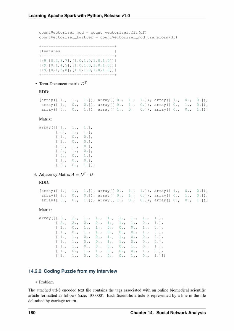
Learning Apache Spark with Python, Release v1.0
countVectorizer_mod = count_vectorizer.fit(df)countVectorizer_twitter = countVectorizer_mod.transform(df)
+-------------------------------+|features |+-------------------------------+|(9,[0,2,3,7],[1.0,1.0,1.0,1.0])||(9,[0,1,4,5],[1.0,1.0,1.0,1.0])||(9,[0,1,6,8],[1.0,1.0,1.0,1.0])|+-------------------------------+
• Term-Document matrix 𝐷𝑇
RDD:
[array([ 1., 1., 1.]), array([ 0., 1., 1.]), array([ 1., 0., 0.]),array([ 1., 0., 0.]), array([ 0., 1., 0.]), array([ 0., 1., 0.]),array([ 0., 0., 1.]), array([ 1., 0., 0.]), array([ 0., 0., 1.])]
Matrix:
array([[ 1., 1., 1.],[ 0., 1., 1.],[ 1., 0., 0.],[ 1., 0., 0.],[ 0., 1., 0.],[ 0., 1., 0.],[ 0., 0., 1.],[ 1., 0., 0.],[ 0., 0., 1.]])
3. Adjacency Matrix 𝐴 = 𝐷𝑇 ·𝐷
RDD:
[array([ 1., 1., 1.]), array([ 0., 1., 1.]), array([ 1., 0., 0.]),array([ 1., 0., 0.]), array([ 0., 1., 0.]), array([ 0., 1., 0.]),array([ 0., 0., 1.]), array([ 1., 0., 0.]), array([ 0., 0., 1.])]
Matrix:
array([[ 3., 2., 1., 1., 1., 1., 1., 1., 1.],[ 2., 2., 0., 0., 1., 1., 1., 0., 1.],[ 1., 0., 1., 1., 0., 0., 0., 1., 0.],[ 1., 0., 1., 1., 0., 0., 0., 1., 0.],[ 1., 1., 0., 0., 1., 1., 0., 0., 0.],[ 1., 1., 0., 0., 1., 1., 0., 0., 0.],[ 1., 1., 0., 0., 0., 0., 1., 0., 1.],[ 1., 0., 1., 1., 0., 0., 0., 1., 0.],[ 1., 1., 0., 0., 0., 0., 1., 0., 1.]])
14.2.2 Coding Puzzle from my interview
• Problem
The attached utf-8 encoded text file contains the tags associated with an online biomedical scientificarticle formatted as follows (size: 100000). Each Scientific article is represented by a line in the filedelimited by carriage return.
180 Chapter 14. Social Network Analysis
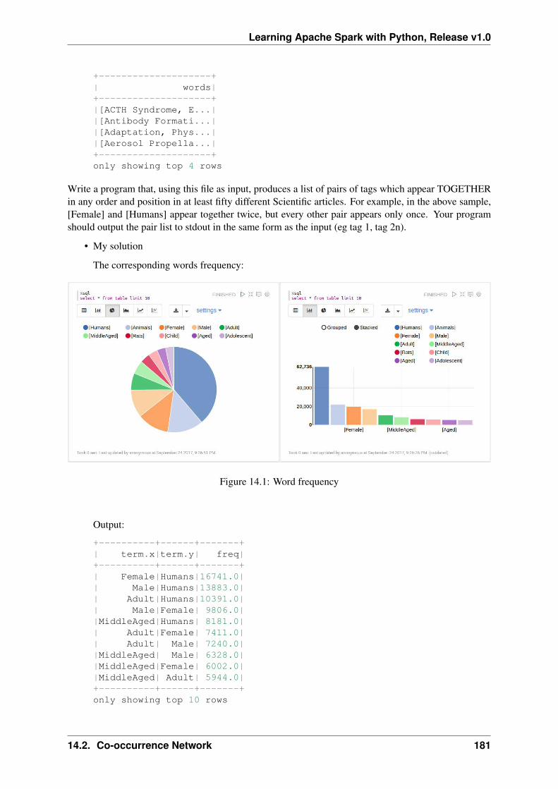
Learning Apache Spark with Python, Release v1.0
+--------------------+| words|+--------------------+|[ACTH Syndrome, E...||[Antibody Formati...||[Adaptation, Phys...||[Aerosol Propella...|+--------------------+only showing top 4 rows
Write a program that, using this file as input, produces a list of pairs of tags which appear TOGETHERin any order and position in at least fifty different Scientific articles. For example, in the above sample,[Female] and [Humans] appear together twice, but every other pair appears only once. Your programshould output the pair list to stdout in the same form as the input (eg tag 1, tag 2n).
• My solution
The corresponding words frequency:
Figure 14.1: Word frequency
Output:
+----------+------+-------+| term.x|term.y| freq|+----------+------+-------+| Female|Humans|16741.0|| Male|Humans|13883.0|| Adult|Humans|10391.0|| Male|Female| 9806.0||MiddleAged|Humans| 8181.0|| Adult|Female| 7411.0|| Adult| Male| 7240.0||MiddleAged| Male| 6328.0||MiddleAged|Female| 6002.0||MiddleAged| Adult| 5944.0|+----------+------+-------+only showing top 10 rows
14.2. Co-occurrence Network 181
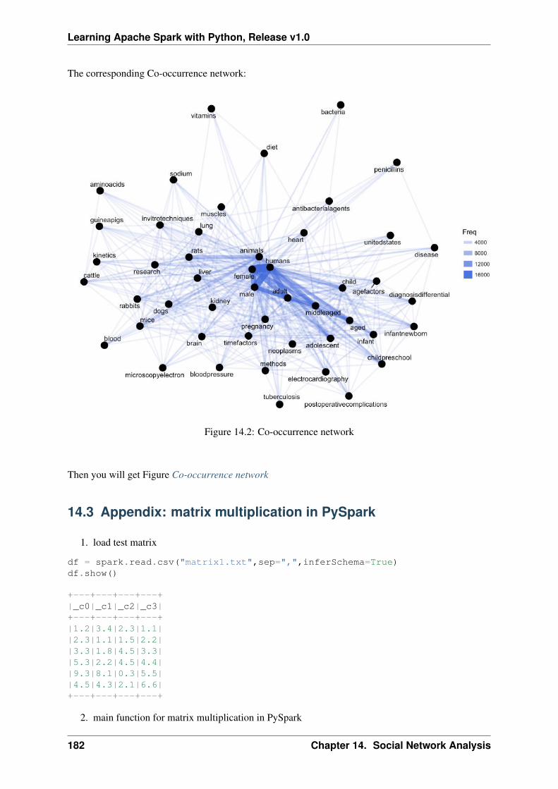
Learning Apache Spark with Python, Release v1.0
The corresponding Co-occurrence network:
Figure 14.2: Co-occurrence network
Then you will get Figure Co-occurrence network
14.3 Appendix: matrix multiplication in PySpark
1. load test matrix
df = spark.read.csv("matrix1.txt",sep=",",inferSchema=True)df.show()
+---+---+---+---+|_c0|_c1|_c2|_c3|+---+---+---+---+|1.2|3.4|2.3|1.1||2.3|1.1|1.5|2.2||3.3|1.8|4.5|3.3||5.3|2.2|4.5|4.4||9.3|8.1|0.3|5.5||4.5|4.3|2.1|6.6|+---+---+---+---+
2. main function for matrix multiplication in PySpark
182 Chapter 14. Social Network Analysis
Learning Apache Spark with Python, Release v1.0
from pyspark.sql import functions as Ffrom functools import reduce# reference: https://stackoverflow.com/questions/44348527/matrix-multiplication-at-a-in-pyspark# do the sum of the multiplication that we want, and get# one data frame for each columncolDFs = []for c2 in df.columns:
colDFs.append( df.select( [ F.sum(df[c1]*df[c2]).alias("op_{0}".format(i)) for i,c1 in enumerate(df.columns) ] ) )# now union those separate data frames to build the "matrix"mtxDF = reduce(lambda a,b: a.select(a.columns).union(b.select(a.columns)), colDFs )mtxDF.show()
+------------------+------------------+------------------+------------------+| op_0| op_1| op_2| op_3|+------------------+------------------+------------------+------------------+| 152.45|118.88999999999999| 57.15|121.44000000000001||118.88999999999999|104.94999999999999| 38.93| 94.71|| 57.15| 38.93|52.540000000000006| 55.99||121.44000000000001| 94.71| 55.99|110.10999999999999|+------------------+------------------+------------------+------------------+
3. Validation with python version
import numpy as npa = np.genfromtxt("matrix1.txt",delimiter=",")np.dot(a.T, a)
array([[152.45, 118.89, 57.15, 121.44],[118.89, 104.95, 38.93, 94.71],[ 57.15, 38.93, 52.54, 55.99],[121.44, 94.71, 55.99, 110.11]])
14.4 Correlation Network
TODO ..
14.4. Correlation Network 183
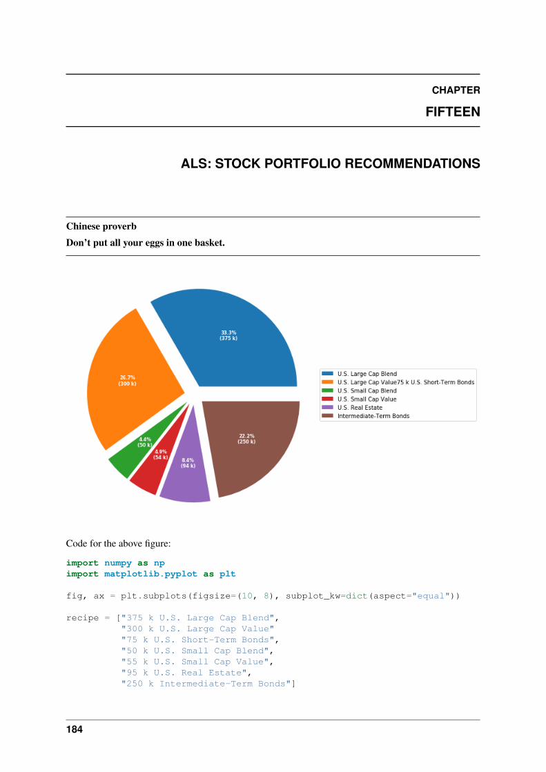
CHAPTER
FIFTEEN
ALS: STOCK PORTFOLIO RECOMMENDATIONS
Chinese proverb
Don’t put all your eggs in one basket.
Code for the above figure:
import numpy as npimport matplotlib.pyplot as plt
fig, ax = plt.subplots(figsize=(10, 8), subplot_kw=dict(aspect="equal"))
recipe = ["375 k U.S. Large Cap Blend","300 k U.S. Large Cap Value""75 k U.S. Short-Term Bonds","50 k U.S. Small Cap Blend","55 k U.S. Small Cap Value","95 k U.S. Real Estate","250 k Intermediate-Term Bonds"]
184
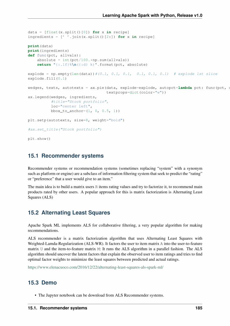
Learning Apache Spark with Python, Release v1.0
data = [float(x.split()[0]) for x in recipe]ingredients = [’ ’.join(x.split()[2:]) for x in recipe]
print(data)print(ingredients)def func(pct, allvals):
absolute = int(pct/100.*np.sum(allvals))return "{:.1f}%\n({:d} k)".format(pct, absolute)
explode = np.empty(len(data))#(0.1, 0.1, 0.1, 0.1, 0.1, 0.1) # explode 1st sliceexplode.fill(0.1)
wedges, texts, autotexts = ax.pie(data, explode=explode, autopct=lambda pct: func(pct, data),textprops=dict(color="w"))
ax.legend(wedges, ingredients,#title="Stock portfolio",loc="center left",bbox_to_anchor=(1, 0, 0.5, 1))
plt.setp(autotexts, size=8, weight="bold")
#ax.set_title("Stock portfolio")
plt.show()
15.1 Recommender systems
Recommender systems or recommendation systems (sometimes replacing “system” with a synonymsuch as platform or engine) are a subclass of information filtering system that seek to predict the “rating”or “preference” that a user would give to an item.”
The main idea is to build a matrix users R items rating values and try to factorize it, to recommend mainproducts rated by other users. A popular approach for this is matrix factorization is Alternating LeastSquares (ALS)
15.2 Alternating Least Squares
Apache Spark ML implements ALS for collaborative filtering, a very popular algorithm for makingrecommendations.
ALS recommender is a matrix factorization algorithm that uses Alternating Least Squares withWeighted-Lamda-Regularization (ALS-WR). It factors the user to item matrix A into the user-to-featurematrix U and the item-to-feature matrix M: It runs the ALS algorithm in a parallel fashion. The ALSalgorithm should uncover the latent factors that explain the observed user to item ratings and tries to findoptimal factor weights to minimize the least squares between predicted and actual ratings.
https://www.elenacuoco.com/2016/12/22/alternating-least-squares-als-spark-ml/
15.3 Demo
• The Jupyter notebook can be download from ALS Recommender systems.
15.1. Recommender systems 185
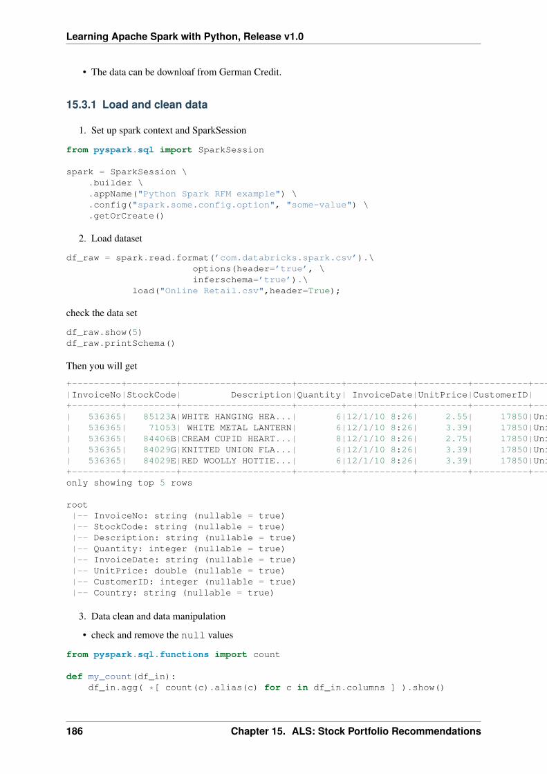
Learning Apache Spark with Python, Release v1.0
• The data can be downloaf from German Credit.
15.3.1 Load and clean data
1. Set up spark context and SparkSession
from pyspark.sql import SparkSession
spark = SparkSession \.builder \.appName("Python Spark RFM example") \.config("spark.some.config.option", "some-value") \.getOrCreate()
2. Load dataset
df_raw = spark.read.format(’com.databricks.spark.csv’).\options(header=’true’, \inferschema=’true’).\
load("Online Retail.csv",header=True);
check the data set
df_raw.show(5)df_raw.printSchema()
Then you will get
+---------+---------+--------------------+--------+------------+---------+----------+--------------+|InvoiceNo|StockCode| Description|Quantity| InvoiceDate|UnitPrice|CustomerID| Country|+---------+---------+--------------------+--------+------------+---------+----------+--------------+| 536365| 85123A|WHITE HANGING HEA...| 6|12/1/10 8:26| 2.55| 17850|United Kingdom|| 536365| 71053| WHITE METAL LANTERN| 6|12/1/10 8:26| 3.39| 17850|United Kingdom|| 536365| 84406B|CREAM CUPID HEART...| 8|12/1/10 8:26| 2.75| 17850|United Kingdom|| 536365| 84029G|KNITTED UNION FLA...| 6|12/1/10 8:26| 3.39| 17850|United Kingdom|| 536365| 84029E|RED WOOLLY HOTTIE...| 6|12/1/10 8:26| 3.39| 17850|United Kingdom|+---------+---------+--------------------+--------+------------+---------+----------+--------------+only showing top 5 rows
root|-- InvoiceNo: string (nullable = true)|-- StockCode: string (nullable = true)|-- Description: string (nullable = true)|-- Quantity: integer (nullable = true)|-- InvoiceDate: string (nullable = true)|-- UnitPrice: double (nullable = true)|-- CustomerID: integer (nullable = true)|-- Country: string (nullable = true)
3. Data clean and data manipulation
• check and remove the null values
from pyspark.sql.functions import count
def my_count(df_in):df_in.agg( *[ count(c).alias(c) for c in df_in.columns ] ).show()
186 Chapter 15. ALS: Stock Portfolio Recommendations
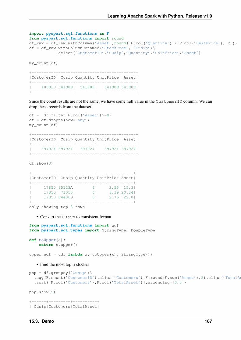
Learning Apache Spark with Python, Release v1.0
import pyspark.sql.functions as Ffrom pyspark.sql.functions import rounddf_raw = df_raw.withColumn(’Asset’,round( F.col(’Quantity’) * F.col(’UnitPrice’), 2 ))df = df_raw.withColumnRenamed(’StockCode’, ’Cusip’)\
.select(’CustomerID’,’Cusip’,’Quantity’,’UnitPrice’,’Asset’)
my_count(df)
+----------+------+--------+---------+------+|CustomerID| Cusip|Quantity|UnitPrice| Asset|+----------+------+--------+---------+------+| 406829|541909| 541909| 541909|541909|+----------+------+--------+---------+------+
Since the count results are not the same, we have some null value in the CustomerID column. We candrop these records from the dataset.
df = df.filter(F.col(’Asset’)>=0)df = df.dropna(how=’any’)my_count(df)
+----------+------+--------+---------+------+|CustomerID| Cusip|Quantity|UnitPrice| Asset|+----------+------+--------+---------+------+| 397924|397924| 397924| 397924|397924|+----------+------+--------+---------+------+
df.show(3)
+----------+------+--------+---------+-----+|CustomerID| Cusip|Quantity|UnitPrice|Asset|+----------+------+--------+---------+-----+| 17850|85123A| 6| 2.55| 15.3|| 17850| 71053| 6| 3.39|20.34|| 17850|84406B| 8| 2.75| 22.0|+----------+------+--------+---------+-----+only showing top 3 rows
• Convert the Cusip to consistent format
from pyspark.sql.functions import udffrom pyspark.sql.types import StringType, DoubleType
def toUpper(s):return s.upper()
upper_udf = udf(lambda x: toUpper(x), StringType())
• Find the most top n stockes
pop = df.groupBy(’Cusip’)\.agg(F.count(’CustomerID’).alias(’Customers’),F.round(F.sum(’Asset’),2).alias(’TotalAsset’))\.sort([F.col(’Customers’),F.col(’TotalAsset’)],ascending=[0,0])
pop.show(5)
+------+---------+----------+| Cusip|Customers|TotalAsset|
15.3. Demo 187
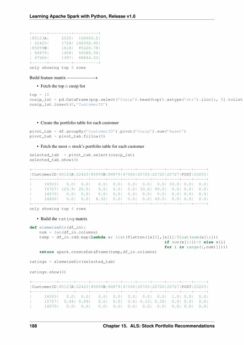
Learning Apache Spark with Python, Release v1.0
+------+---------+----------+|85123A| 2035| 100603.5|| 22423| 1724| 142592.95||85099B| 1618| 85220.78|| 84879| 1408| 56580.34|| 47566| 1397| 68844.33|+------+---------+----------+only showing top 5 rows
Build feature matrix ——————-+
• Fetch the top n cusip list
top = 10cusip_lst = pd.DataFrame(pop.select(’Cusip’).head(top)).astype(’str’).iloc[:, 0].tolist()cusip_lst.insert(0,’CustomerID’)
• Create the portfolio table for each customer
pivot_tab = df.groupBy(’CustomerID’).pivot(’Cusip’).sum(’Asset’)pivot_tab = pivot_tab.fillna(0)
• Fetch the most n stock’s portfolio table for each customer
selected_tab = pivot_tab.select(cusip_lst)selected_tab.show(4)
+----------+------+-----+------+-----+-----+-----+-----+-----+----+-----+|CustomerID|85123A|22423|85099B|84879|47566|20725|22720|20727|POST|23203|+----------+------+-----+------+-----+-----+-----+-----+-----+----+-----+| 16503| 0.0| 0.0| 0.0| 0.0| 0.0| 0.0| 0.0| 33.0| 0.0| 0.0|| 15727| 123.9| 25.5| 0.0| 0.0| 0.0| 33.0| 99.0| 0.0| 0.0| 0.0|| 14570| 0.0| 0.0| 0.0| 0.0| 0.0| 0.0| 0.0| 0.0| 0.0| 0.0|| 14450| 0.0| 0.0| 8.32| 0.0| 0.0| 0.0| 49.5| 0.0| 0.0| 0.0|+----------+------+-----+------+-----+-----+-----+-----+-----+----+-----+only showing top 4 rows
• Build the rating matrix
def elemwiseDiv(df_in):num = len(df_in.columns)temp = df_in.rdd.map(lambda x: list(flatten([x[0],[x[i]/float(sum(x[1:]))
if sum(x[1:])>0 else x[i]for i in range(1,num)]])))
return spark.createDataFrame(temp,df_in.columns)
ratings = elemwiseDiv(selected_tab)
ratings.show(4)
+----------+------+-----+------+-----+-----+-----+-----+-----+----+-----+|CustomerID|85123A|22423|85099B|84879|47566|20725|22720|20727|POST|23203|+----------+------+-----+------+-----+-----+-----+-----+-----+----+-----+| 16503| 0.0| 0.0| 0.0| 0.0| 0.0| 0.0| 0.0| 1.0| 0.0| 0.0|| 15727| 0.44| 0.09| 0.0| 0.0| 0.0| 0.12| 0.35| 0.0| 0.0| 0.0|| 14570| 0.0| 0.0| 0.0| 0.0| 0.0| 0.0| 0.0| 0.0| 0.0| 0.0|
188 Chapter 15. ALS: Stock Portfolio Recommendations
Learning Apache Spark with Python, Release v1.0
| 14450| 0.0| 0.0| 0.14| 0.0| 0.0| 0.0| 0.86| 0.0| 0.0| 0.0|+----------+------+-----+------+-----+-----+-----+-----+-----+----+-----+
• Convert rating matrix to long table
from pyspark.sql.functions import array, col, explode, struct, lit
def to_long(df, by):"""reference: https://stackoverflow.com/questions/37864222/transpose-column-to-row-with-spark"""
# Filter dtypes and split into column names and type descriptioncols, dtypes = zip(*((c, t) for (c, t) in df.dtypes if c not in by))# Spark SQL supports only homogeneous columnsassert len(set(dtypes)) == 1, "All columns have to be of the same type"
# Create and explode an array of (column_name, column_value) structskvs = explode(array([
struct(lit(c).alias("Cusip"), col(c).alias("rating")) for c in cols])).alias("kvs")
df_all = to_long(ratings,[’CustomerID’])df_all.show(5)
+----------+------+------+|CustomerID| Cusip|rating|+----------+------+------+| 16503|85123A| 0.0|| 16503| 22423| 0.0|| 16503|85099B| 0.0|| 16503| 84879| 0.0|| 16503| 47566| 0.0|+----------+------+------+only showing top 5 rows
• Convert the string Cusip to numerical index
from pyspark.ml.feature import StringIndexer# Index labels, adding metadata to the label columnlabelIndexer = StringIndexer(inputCol=’Cusip’,
outputCol=’indexedCusip’).fit(df_all)df_all = labelIndexer.transform(df_all)
df_all.show(5, True)df_all.printSchema()
+----------+------+------+------------+|CustomerID| Cusip|rating|indexedCusip|+----------+------+------+------------+| 16503|85123A| 0.0| 6.0|| 16503| 22423| 0.0| 9.0|| 16503|85099B| 0.0| 5.0|| 16503| 84879| 0.0| 1.0|| 16503| 47566| 0.0| 0.0|+----------+------+------+------------+only showing top 5 rows
15.3. Demo 189
Learning Apache Spark with Python, Release v1.0
root|-- CustomerID: long (nullable = true)|-- Cusip: string (nullable = false)|-- rating: double (nullable = true)|-- indexedCusip: double (nullable = true)
15.3.2 Train model
• build train and test dataset
train, test = df_all.randomSplit([0.8,0.2])
train.show(5)test.show(5)
+----------+-----+------------+-------------------+|CustomerID|Cusip|indexedCusip| rating|+----------+-----+------------+-------------------+| 12940|20725| 2.0| 0.0|| 12940|20727| 4.0| 0.0|| 12940|22423| 9.0|0.49990198000392083|| 12940|22720| 3.0| 0.0|| 12940|23203| 7.0| 0.0|+----------+-----+------------+-------------------+only showing top 5 rows
+----------+-----+------------+------------------+|CustomerID|Cusip|indexedCusip| rating|+----------+-----+------------+------------------+| 12940|84879| 1.0|0.1325230346990786|| 13285|20725| 2.0|0.2054154995331466|| 13285|20727| 4.0|0.2054154995331466|| 13285|47566| 0.0| 0.0|| 13623|23203| 7.0| 0.0|+----------+-----+------------+------------------+only showing top 5 rows
• train model
import itertoolsfrom math import sqrtfrom operator import addimport sysfrom pyspark.ml.recommendation import ALS
from pyspark.ml.evaluation import RegressionEvaluator
evaluator = RegressionEvaluator(metricName="rmse", labelCol="rating",predictionCol="prediction")
def computeRmse(model, data):"""Compute RMSE (Root mean Squared Error)."""predictions = model.transform(data)rmse = evaluator.evaluate(predictions)print("Root-mean-square error = " + str(rmse))
190 Chapter 15. ALS: Stock Portfolio Recommendations
Learning Apache Spark with Python, Release v1.0
return rmse
#train models and evaluate them on the validation set
ranks = [4,5]lambdas = [0.05]numIters = [30]bestModel = NonebestValidationRmse = float("inf")bestRank = 0bestLambda = -1.0bestNumIter = -1
val = test.na.drop()for rank, lmbda, numIter in itertools.product(ranks, lambdas, numIters):
als = ALS(rank=rank, maxIter=numIter, regParam=lmbda, numUserBlocks=10, numItemBlocks=10, implicitPrefs=False,alpha=1.0,userCol="CustomerID", itemCol="indexedCusip", seed=1, ratingCol="rating", nonnegative=True)
model=als.fit(train)
validationRmse = computeRmse(model, val)print("RMSE (validation) = %f for the model trained with " % validationRmse + \
"rank = %d, lambda = %.1f, and numIter = %d." % (rank, lmbda, numIter))if (validationRmse, bestValidationRmse):
bestModel = modelbestValidationRmse = validationRmsebestRank = rankbestLambda = lmbdabestNumIter = numIter
model = bestModel
15.3.3 Make prediction
• make prediction
topredict=test[test[’rating’]==0]
predictions=model.transform(topredict)predictions.filter(predictions.prediction>0)\
.sort([F.col(’CustomerID’),F.col(’Cusip’)],ascending=[0,0]).show(5)
+----------+------+------------+------+------------+|CustomerID| Cusip|indexedCusip|rating| prediction|+----------+------+------------+------+------------+| 18283| 47566| 0.0| 0.0| 0.01625076|| 18282|85123A| 6.0| 0.0| 0.057172246|| 18282| 84879| 1.0| 0.0| 0.059531752|| 18282| 23203| 7.0| 0.0| 0.010502596|| 18282| 22720| 3.0| 0.0| 0.053893942|+----------+------+------------+------+------------+only showing top 5 rows
15.3. Demo 191
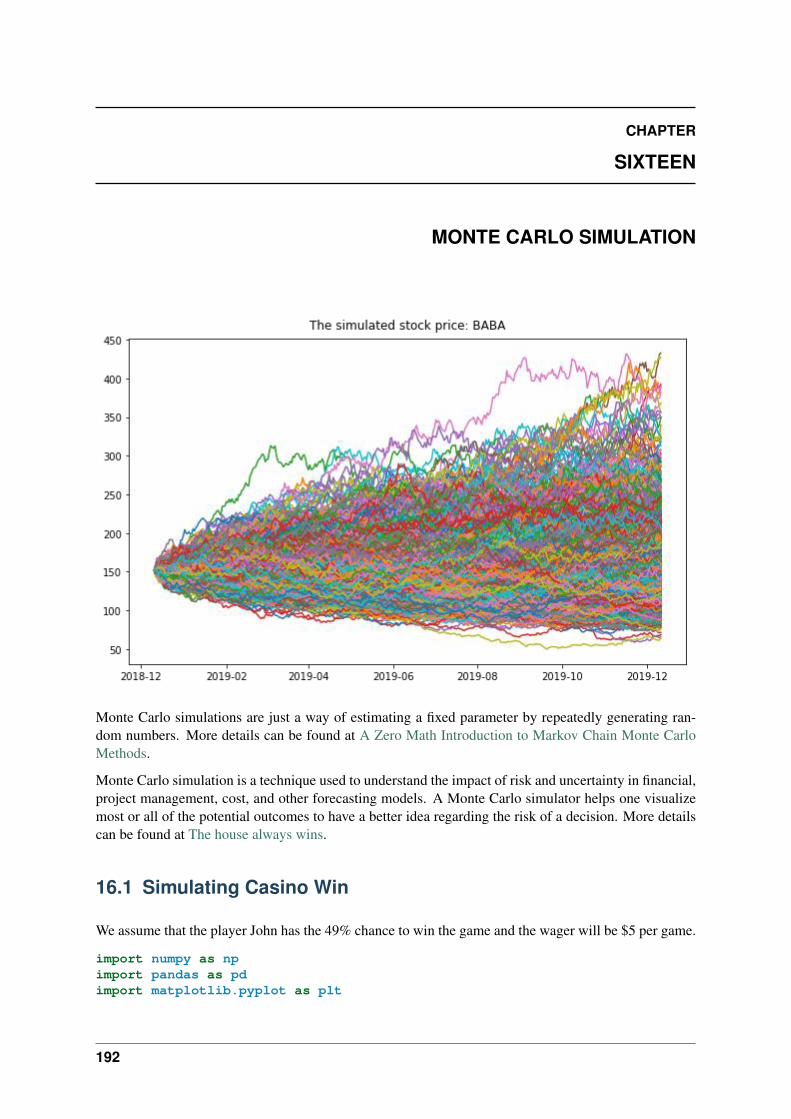
CHAPTER
SIXTEEN
MONTE CARLO SIMULATION
Monte Carlo simulations are just a way of estimating a fixed parameter by repeatedly generating ran-dom numbers. More details can be found at A Zero Math Introduction to Markov Chain Monte CarloMethods.
Monte Carlo simulation is a technique used to understand the impact of risk and uncertainty in financial,project management, cost, and other forecasting models. A Monte Carlo simulator helps one visualizemost or all of the potential outcomes to have a better idea regarding the risk of a decision. More detailscan be found at The house always wins.
16.1 Simulating Casino Win
We assume that the player John has the 49% chance to win the game and the wager will be $5 per game.
import numpy as npimport pandas as pdimport matplotlib.pyplot as plt
192
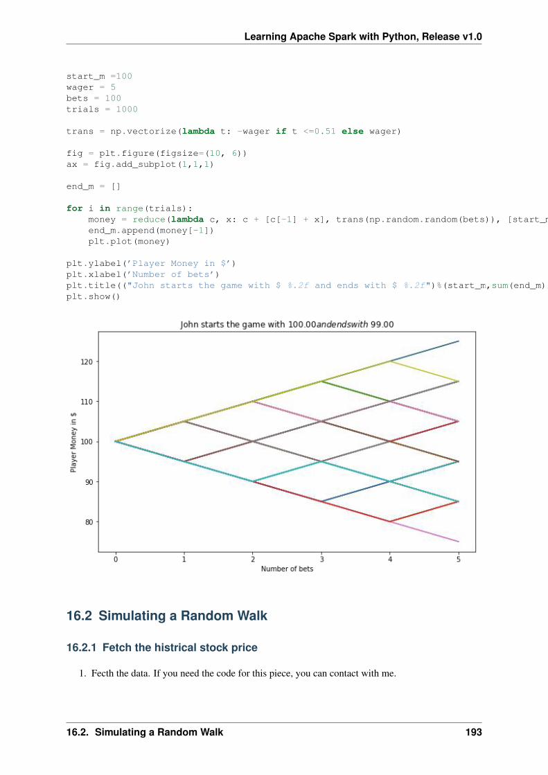
Learning Apache Spark with Python, Release v1.0
start_m =100wager = 5bets = 100trials = 1000
trans = np.vectorize(lambda t: -wager if t <=0.51 else wager)
fig = plt.figure(figsize=(10, 6))ax = fig.add_subplot(1,1,1)
end_m = []
for i in range(trials):money = reduce(lambda c, x: c + [c[-1] + x], trans(np.random.random(bets)), [start_m])end_m.append(money[-1])plt.plot(money)
plt.ylabel(’Player Money in $’)plt.xlabel(’Number of bets’)plt.title(("John starts the game with $ %.2f and ends with $ %.2f")%(start_m,sum(end_m)/len(end_m)))plt.show()
16.2 Simulating a Random Walk
16.2.1 Fetch the histrical stock price
1. Fecth the data. If you need the code for this piece, you can contact with me.
16.2. Simulating a Random Walk 193
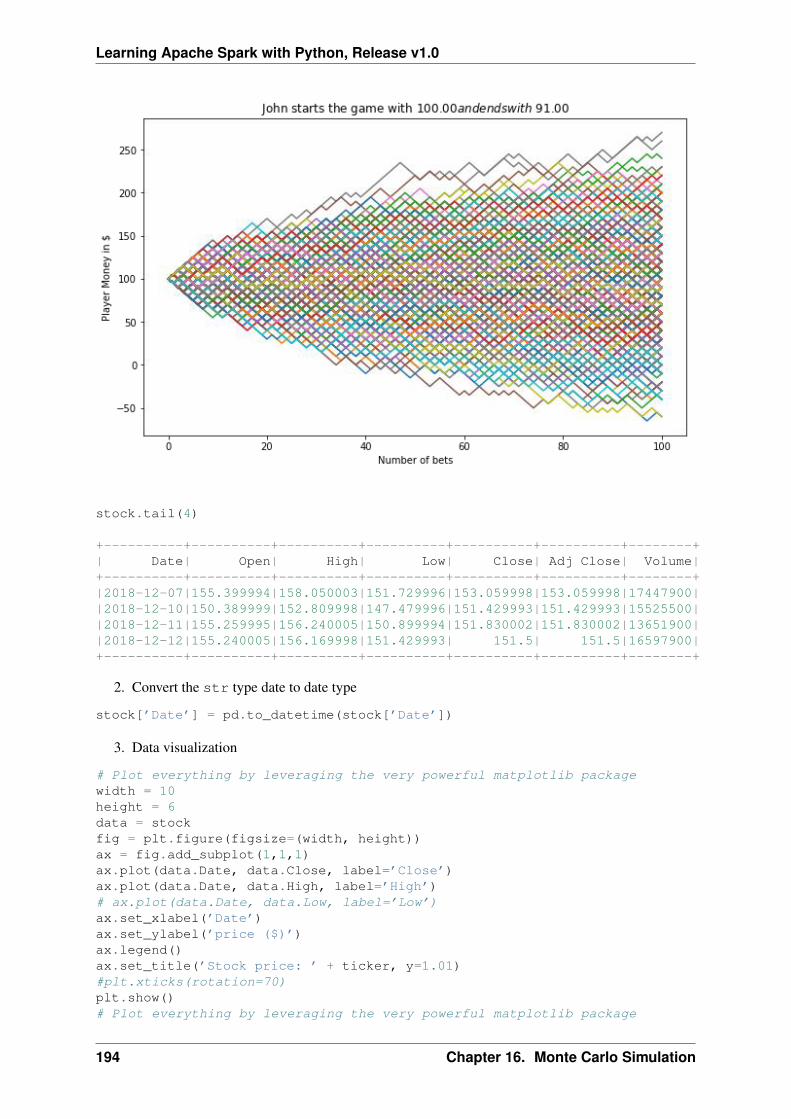
Learning Apache Spark with Python, Release v1.0
stock.tail(4)
+----------+----------+----------+----------+----------+----------+--------+| Date| Open| High| Low| Close| Adj Close| Volume|+----------+----------+----------+----------+----------+----------+--------+|2018-12-07|155.399994|158.050003|151.729996|153.059998|153.059998|17447900||2018-12-10|150.389999|152.809998|147.479996|151.429993|151.429993|15525500||2018-12-11|155.259995|156.240005|150.899994|151.830002|151.830002|13651900||2018-12-12|155.240005|156.169998|151.429993| 151.5| 151.5|16597900|+----------+----------+----------+----------+----------+----------+--------+
2. Convert the str type date to date type
stock[’Date’] = pd.to_datetime(stock[’Date’])
3. Data visualization
# Plot everything by leveraging the very powerful matplotlib packagewidth = 10height = 6data = stockfig = plt.figure(figsize=(width, height))ax = fig.add_subplot(1,1,1)ax.plot(data.Date, data.Close, label=’Close’)ax.plot(data.Date, data.High, label=’High’)# ax.plot(data.Date, data.Low, label=’Low’)ax.set_xlabel(’Date’)ax.set_ylabel(’price ($)’)ax.legend()ax.set_title(’Stock price: ’ + ticker, y=1.01)#plt.xticks(rotation=70)plt.show()# Plot everything by leveraging the very powerful matplotlib package
194 Chapter 16. Monte Carlo Simulation
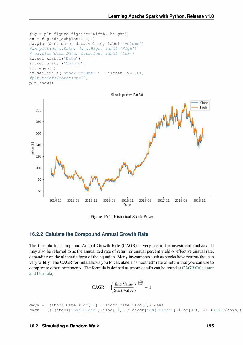
Learning Apache Spark with Python, Release v1.0
fig = plt.figure(figsize=(width, height))ax = fig.add_subplot(1,1,1)ax.plot(data.Date, data.Volume, label=’Volume’)#ax.plot(data.Date, data.High, label=’High’)# ax.plot(data.Date, data.Low, label=’Low’)ax.set_xlabel(’Date’)ax.set_ylabel(’Volume’)ax.legend()ax.set_title(’Stock volume: ’ + ticker, y=1.01)#plt.xticks(rotation=70)plt.show()
Figure 16.1: Historical Stock Price
16.2.2 Calulate the Compound Annual Growth Rate
The formula for Compound Annual Growth Rate (CAGR) is very useful for investment analysis. Itmay also be referred to as the annualized rate of return or annual percent yield or effective annual rate,depending on the algebraic form of the equation. Many investments such as stocks have returns that canvary wildly. The CAGR formula allows you to calculate a “smoothed” rate of return that you can use tocompare to other investments. The formula is defined as (more details can be found at CAGR Calculatorand Formula)
CAGR =
(︂End ValueStart Value
)︂ 365Days
− 1
days = (stock.Date.iloc[-1] - stock.Date.iloc[0]).dayscagr = ((((stock[’Adj Close’].iloc[-1]) / stock[’Adj Close’].iloc[0])) ** (365.0/days)) - 1
16.2. Simulating a Random Walk 195
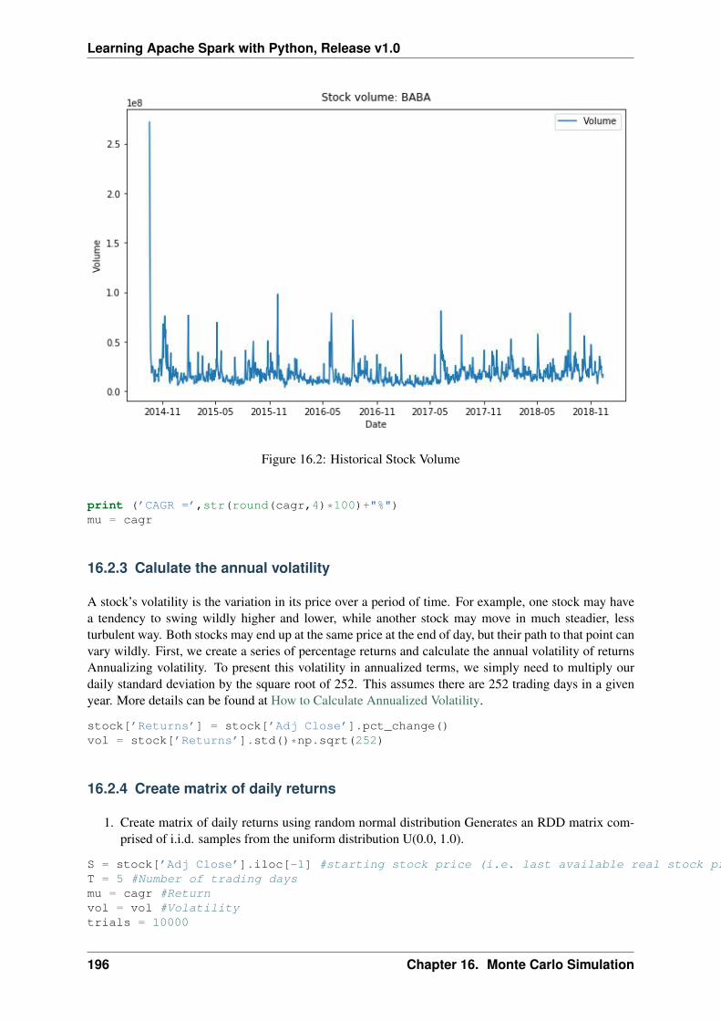
Learning Apache Spark with Python, Release v1.0
Figure 16.2: Historical Stock Volume
print (’CAGR =’,str(round(cagr,4)*100)+"%")mu = cagr
16.2.3 Calulate the annual volatility
A stock’s volatility is the variation in its price over a period of time. For example, one stock may havea tendency to swing wildly higher and lower, while another stock may move in much steadier, lessturbulent way. Both stocks may end up at the same price at the end of day, but their path to that point canvary wildly. First, we create a series of percentage returns and calculate the annual volatility of returnsAnnualizing volatility. To present this volatility in annualized terms, we simply need to multiply ourdaily standard deviation by the square root of 252. This assumes there are 252 trading days in a givenyear. More details can be found at How to Calculate Annualized Volatility.
stock[’Returns’] = stock[’Adj Close’].pct_change()vol = stock[’Returns’].std()*np.sqrt(252)
16.2.4 Create matrix of daily returns
1. Create matrix of daily returns using random normal distribution Generates an RDD matrix com-prised of i.i.d. samples from the uniform distribution U(0.0, 1.0).
S = stock[’Adj Close’].iloc[-1] #starting stock price (i.e. last available real stock price)T = 5 #Number of trading daysmu = cagr #Returnvol = vol #Volatilitytrials = 10000
196 Chapter 16. Monte Carlo Simulation
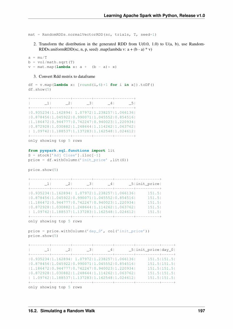
Learning Apache Spark with Python, Release v1.0
mat = RandomRDDs.normalVectorRDD(sc, trials, T, seed=1)
2. Transform the distribution in the generated RDD from U(0.0, 1.0) to U(a, b), use Random-RDDs.uniformRDD(sc, n, p, seed) .map(lambda v: a + (b - a) * v)
a = mu/Tb = vol/math.sqrt(T)v = mat.map(lambda x: a + (b - a)* x)
3. Convert Rdd mstrix to dataframe
df = v.map(lambda x: [round(i,6)+1 for i in x]).toDF()df.show(5)
+--------+--------+--------+--------+--------+| _1| _2| _3| _4| _5|+--------+--------+--------+--------+--------+|0.935234|1.162894| 1.07972|1.238257|1.066136||0.878456|1.045922|0.990071|1.045552|0.854516||1.186472|0.944777|0.742247|0.940023|1.220934||0.872928|1.030882|1.248644|1.114262|1.063762|| 1.09742|1.188537|1.137283|1.162548|1.024612|+--------+--------+--------+--------+--------+only showing top 5 rows
from pyspark.sql.functions import litS = stock[’Adj Close’].iloc[-1]price = df.withColumn(’init_price’ ,lit(S))
price.show(5)
+--------+--------+--------+--------+--------+----------+| _1| _2| _3| _4| _5|init_price|+--------+--------+--------+--------+--------+----------+|0.935234|1.162894| 1.07972|1.238257|1.066136| 151.5||0.878456|1.045922|0.990071|1.045552|0.854516| 151.5||1.186472|0.944777|0.742247|0.940023|1.220934| 151.5||0.872928|1.030882|1.248644|1.114262|1.063762| 151.5|| 1.09742|1.188537|1.137283|1.162548|1.024612| 151.5|+--------+--------+--------+--------+--------+----------+only showing top 5 rows
price = price.withColumn(’day_0’, col(’init_price’))price.show(5)
+--------+--------+--------+--------+--------+----------+-----+| _1| _2| _3| _4| _5|init_price|day_0|+--------+--------+--------+--------+--------+----------+-----+|0.935234|1.162894| 1.07972|1.238257|1.066136| 151.5|151.5||0.878456|1.045922|0.990071|1.045552|0.854516| 151.5|151.5||1.186472|0.944777|0.742247|0.940023|1.220934| 151.5|151.5||0.872928|1.030882|1.248644|1.114262|1.063762| 151.5|151.5|| 1.09742|1.188537|1.137283|1.162548|1.024612| 151.5|151.5|+--------+--------+--------+--------+--------+----------+-----+only showing top 5 rows
16.2. Simulating a Random Walk 197
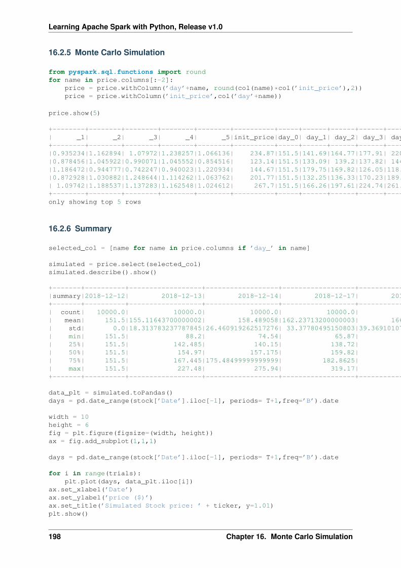
Learning Apache Spark with Python, Release v1.0
16.2.5 Monte Carlo Simulation
from pyspark.sql.functions import roundfor name in price.columns[:-2]:
price = price.withColumn(’day’+name, round(col(name)*col(’init_price’),2))price = price.withColumn(’init_price’,col(’day’+name))
price.show(5)
+--------+--------+--------+--------+--------+----------+-----+------+------+------+------+------+| _1| _2| _3| _4| _5|init_price|day_0| day_1| day_2| day_3| day_4| day_5|+--------+--------+--------+--------+--------+----------+-----+------+------+------+------+------+|0.935234|1.162894| 1.07972|1.238257|1.066136| 234.87|151.5|141.69|164.77|177.91| 220.3|234.87||0.878456|1.045922|0.990071|1.045552|0.854516| 123.14|151.5|133.09| 139.2|137.82| 144.1|123.14||1.186472|0.944777|0.742247|0.940023|1.220934| 144.67|151.5|179.75|169.82|126.05|118.49|144.67||0.872928|1.030882|1.248644|1.114262|1.063762| 201.77|151.5|132.25|136.33|170.23|189.68|201.77|| 1.09742|1.188537|1.137283|1.162548|1.024612| 267.7|151.5|166.26|197.61|224.74|261.27| 267.7|+--------+--------+--------+--------+--------+----------+-----+------+------+------+------+------+only showing top 5 rows
16.2.6 Summary
selected_col = [name for name in price.columns if ’day_’ in name]
simulated = price.select(selected_col)simulated.describe().show()
+-------+----------+------------------+------------------+------------------+------------------+------------------+|summary|2018-12-12| 2018-12-13| 2018-12-14| 2018-12-17| 2018-12-18| 2018-12-19|+-------+----------+------------------+------------------+------------------+------------------+------------------+| count| 10000.0| 10000.0| 10000.0| 10000.0| 10000.0| 10000.0|| mean| 151.5|155.11643700000002| 158.489058|162.23713200000003| 166.049375| 170.006525|| std| 0.0|18.313783237787845|26.460919262517276| 33.37780495150803|39.369101074463416|45.148120695490846|| min| 151.5| 88.2| 74.54| 65.87| 68.21| 58.25|| 25%| 151.5| 142.485| 140.15| 138.72| 138.365| 137.33|| 50%| 151.5| 154.97| 157.175| 159.82| 162.59|165.04500000000002|| 75%| 151.5| 167.445|175.48499999999999| 182.8625| 189.725| 196.975|| max| 151.5| 227.48| 275.94| 319.17| 353.59| 403.68|+-------+----------+------------------+------------------+------------------+------------------+------------------+
data_plt = simulated.toPandas()days = pd.date_range(stock[’Date’].iloc[-1], periods= T+1,freq=’B’).date
width = 10height = 6fig = plt.figure(figsize=(width, height))ax = fig.add_subplot(1,1,1)
days = pd.date_range(stock[’Date’].iloc[-1], periods= T+1,freq=’B’).date
for i in range(trials):plt.plot(days, data_plt.iloc[i])
ax.set_xlabel(’Date’)ax.set_ylabel(’price ($)’)ax.set_title(’Simulated Stock price: ’ + ticker, y=1.01)plt.show()
198 Chapter 16. Monte Carlo Simulation
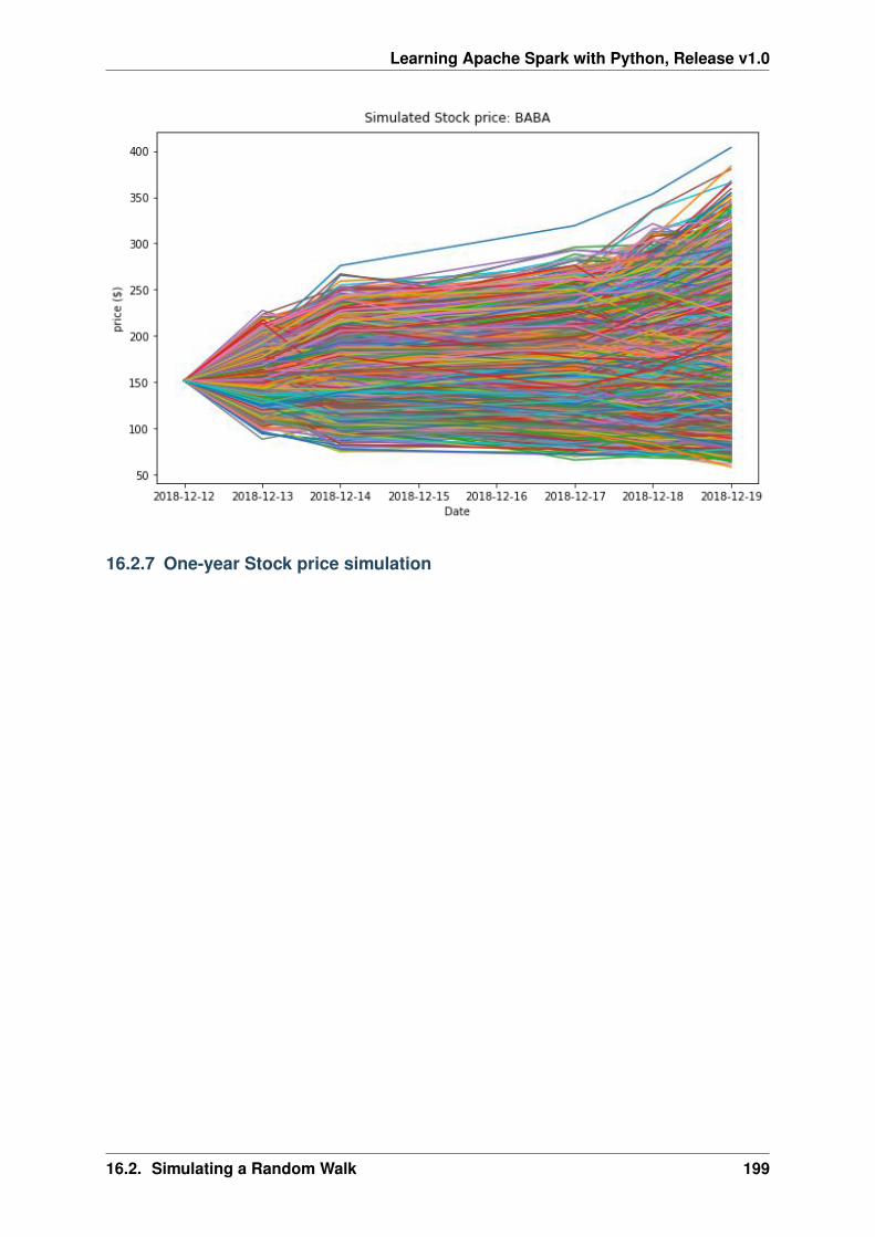
Learning Apache Spark with Python, Release v1.0
16.2.7 One-year Stock price simulation
16.2. Simulating a Random Walk 199
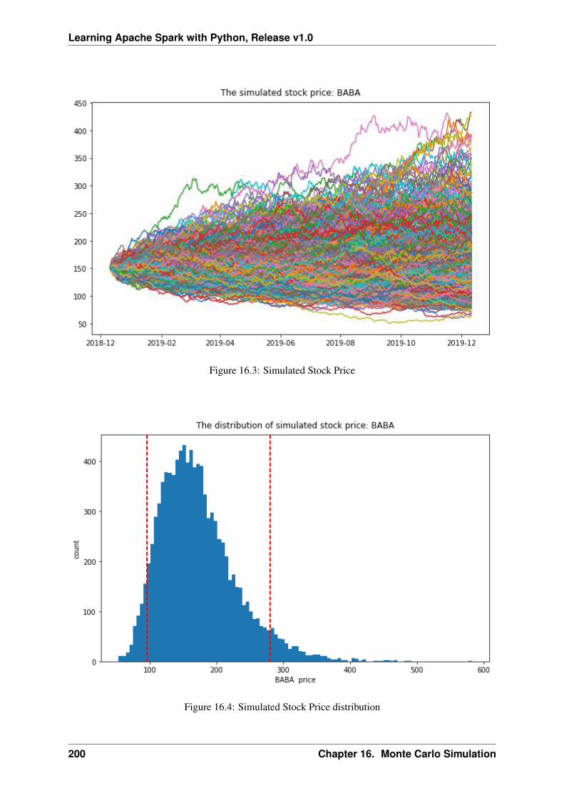
Learning Apache Spark with Python, Release v1.0
Figure 16.3: Simulated Stock Price
Figure 16.4: Simulated Stock Price distribution
200 Chapter 16. Monte Carlo Simulation

CHAPTER
SEVENTEEN
MARKOV CHAIN MONTE CARLO
Monte Carlo simulations are just a way of estimating a fixed parameter by repeatedly generating ran-dom numbers. More details can be found at A Zero Math Introduction to Markov Chain Monte CarloMethods.
Markov Chain Monte Carlo (MCMC) methods are used to approximate the posterior distribution of aparameter of interest by random sampling in a probabilistic space. More details can be found at A ZeroMath Introduction to Markov Chain Monte Carlo Methods.
TODO ..
201
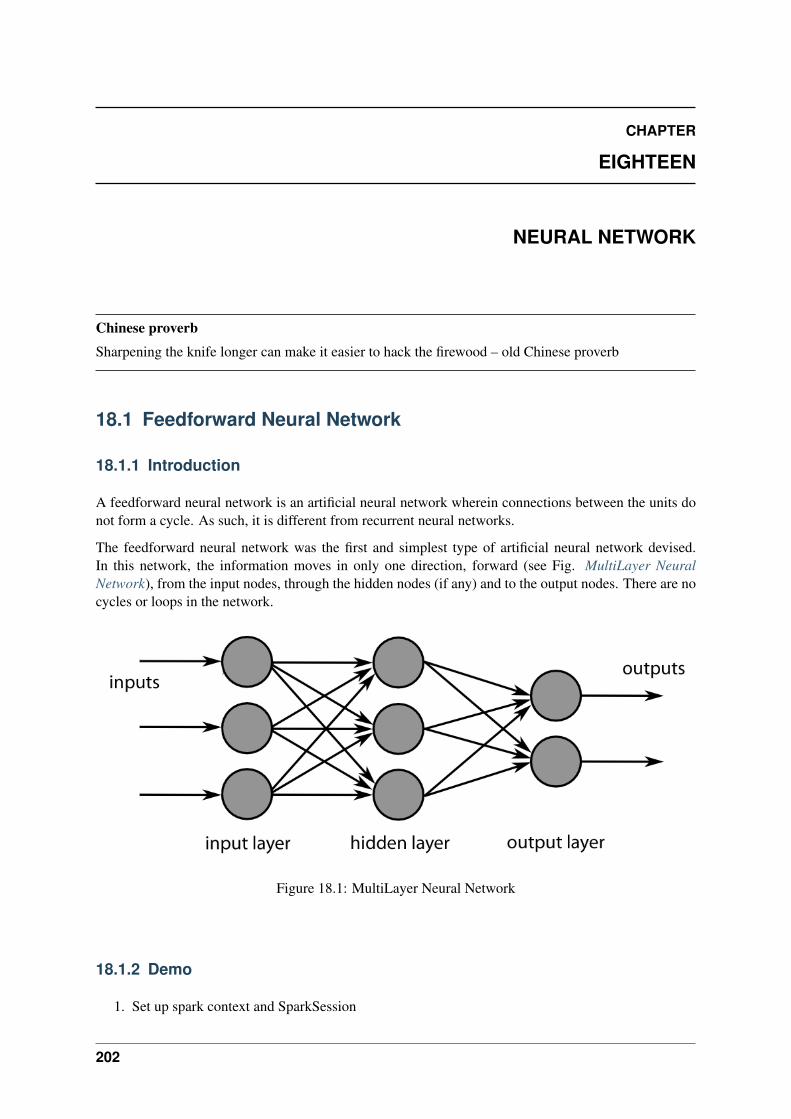
CHAPTER
EIGHTEEN
NEURAL NETWORK
Chinese proverb
Sharpening the knife longer can make it easier to hack the firewood – old Chinese proverb
18.1 Feedforward Neural Network
18.1.1 Introduction
A feedforward neural network is an artificial neural network wherein connections between the units donot form a cycle. As such, it is different from recurrent neural networks.
The feedforward neural network was the first and simplest type of artificial neural network devised.In this network, the information moves in only one direction, forward (see Fig. MultiLayer NeuralNetwork), from the input nodes, through the hidden nodes (if any) and to the output nodes. There are nocycles or loops in the network.
Figure 18.1: MultiLayer Neural Network
18.1.2 Demo
1. Set up spark context and SparkSession
202
Learning Apache Spark with Python, Release v1.0
from pyspark.sql import SparkSession
spark = SparkSession \.builder \.appName("Python Spark Feedforward neural network example") \.config("spark.some.config.option", "some-value") \.getOrCreate()
2. Load dataset
+-----+--------+------+-----+---------+----+-----+-------+----+---------+-------+-------+|fixed|volatile|citric|sugar|chlorides|free|total|density| pH|sulphates|alcohol|quality|+-----+--------+------+-----+---------+----+-----+-------+----+---------+-------+-------+| 7.4| 0.7| 0.0| 1.9| 0.076|11.0| 34.0| 0.9978|3.51| 0.56| 9.4| 5|| 7.8| 0.88| 0.0| 2.6| 0.098|25.0| 67.0| 0.9968| 3.2| 0.68| 9.8| 5|| 7.8| 0.76| 0.04| 2.3| 0.092|15.0| 54.0| 0.997|3.26| 0.65| 9.8| 5|| 11.2| 0.28| 0.56| 1.9| 0.075|17.0| 60.0| 0.998|3.16| 0.58| 9.8| 6|| 7.4| 0.7| 0.0| 1.9| 0.076|11.0| 34.0| 0.9978|3.51| 0.56| 9.4| 5|+-----+--------+------+-----+---------+----+-----+-------+----+---------+-------+-------+only showing top 5 rows
3. change categorical variable size
# Convert to float formatdef string_to_float(x):
return float(x)
#def condition(r):
if (0<= r <= 4):label = "low"
elif(4< r <= 6):label = "medium"
else:label = "high"
return label
from pyspark.sql.functions import udffrom pyspark.sql.types import StringType, DoubleTypestring_to_float_udf = udf(string_to_float, DoubleType())quality_udf = udf(lambda x: condition(x), StringType())df= df.withColumn("quality", quality_udf("quality"))
4. Convert the data to dense vector
# convert the data to dense vectordef transData(data):
return data.rdd.map(lambda r: [r[-1], Vectors.dense(r[:-1])]).\toDF([’label’,’features’])
from pyspark.sql import Rowfrom pyspark.ml.linalg import Vectors
data= transData(df)data.show()
5. Split the data into training and test sets (40% held out for testing)
18.1. Feedforward Neural Network 203
Learning Apache Spark with Python, Release v1.0
# Split the data into train and test(trainingData, testData) = data.randomSplit([0.6, 0.4])
6. Train neural network
# specify layers for the neural network:# input layer of size 11 (features), two intermediate of size 5 and 4# and output of size 7 (classes)layers = [11, 5, 4, 4, 3 , 7]
# create the trainer and set its parametersFNN = MultilayerPerceptronClassifier(labelCol="indexedLabel", \
featuresCol="indexedFeatures",\maxIter=100, layers=layers, \blockSize=128, seed=1234)
# Convert indexed labels back to original labels.labelConverter = IndexToString(inputCol="prediction", outputCol="predictedLabel",
labels=labelIndexer.labels)# Chain indexers and forest in a Pipelinefrom pyspark.ml import Pipelinepipeline = Pipeline(stages=[labelIndexer, featureIndexer, FNN, labelConverter])# train the model# Train model. This also runs the indexers.model = pipeline.fit(trainingData)
7. Make predictions
# Make predictions.predictions = model.transform(testData)# Select example rows to display.predictions.select("features","label","predictedLabel").show(5)
8. Evaluation
# Select (prediction, true label) and compute test errorevaluator = MulticlassClassificationEvaluator(
labelCol="indexedLabel", predictionCol="prediction", metricName="accuracy")accuracy = evaluator.evaluate(predictions)print("Predictions accuracy = %g, Test Error = %g" % (accuracy,(1.0 - accuracy)))
204 Chapter 18. Neural Network
CHAPTER
NINETEEN
MY PYSPARK PACKAGE
It’s super easy to wrap your own package in Python. I packed some functions which I frequently used inmy daily work. You can download and install it from My PySpark Package. The hierarchical structureand the directory structure of this package are as follows.
19.1 Hierarchical Structure
|-- build| |-- bdist.linux-x86_64| |-- lib.linux-x86_64-2.7| |-- PySparkTools| |-- __init__.py| |-- Manipulation| | |-- DataManipulation.py| | |-- __init__.py| |-- Visualization| |-- __init__.py| |-- PyPlots.py|-- dist| |-- PySParkTools-1.0-py2.7.egg|-- __init__.py|-- PySparkTools| |-- __init__.py| |-- Manipulation| | |-- DataManipulation.py| | |-- __init__.py| |-- Visualization| |-- __init__.py| |-- PyPlots.py| |-- PyPlots.pyc|-- PySParkTools.egg-info| |-- dependency_links.txt| |-- PKG-INFO| |-- requires.txt| |-- SOURCES.txt| |-- top_level.txt|-- README.md|-- requirements.txt|-- setup.py|-- test
|-- spark-warehouse|-- test1.py|-- test2.py
205
Learning Apache Spark with Python, Release v1.0
From the above hierarchical structure, you will find that you have to have __init__.py in eachdirectory. I will explain the __init__.py file with the example below:
19.2 Set Up
from setuptools import setup, find_packages
try:with open("README.md") as f:
long_description = f.read()except IOError:
long_description = ""
try:with open("requirements.txt") as f:
requirements = [x.strip() for x in f.read().splitlines() if x.strip()]except IOError:
requirements = []
setup(name=’PySParkTools’,install_requires=requirements,
version=’1.0’,description=’Python Spark Tools’,author=’Wenqiang Feng’,author_email=’[email protected]’,url=’https://github.com/runawayhorse001/PySparkTools’,packages=find_packages(),long_description=long_description)
19.3 ReadMe
# PySparkTools
This is my PySpark Tools. If you want to colne and install it, you can use
- clone
‘‘‘{bash}git clone [email protected]:runawayhorse001/PySparkTools.git‘‘‘- install
‘‘‘{bash}cd PySparkToolspip install -r requirements.txtpython setup.py install‘‘‘
- test
‘‘‘{bash}cd PySparkTools/test
206 Chapter 19. My PySpark Package

Learning Apache Spark with Python, Release v1.0
python test1.py‘‘‘
19.3. ReadMe 207

CHAPTER
TWENTY
MAIN REFERENCE
208
BIBLIOGRAPHY
[Bird2009] 19. Bird, E. Klein, and E. Loper. Natural language processing with Python: analyzing textwith the natural language toolkit. O’Reilly Media, Inc., 2009.
[Feng2017] 23. Feng and M. Chen. Learning Apache Spark, Github 2017.
[Karau2015] 8. Karau, A. Konwinski, P. Wendell and M. Zaharia. Learning Spark: Lightning-FastBig Data Analysis. O’Reilly Media, Inc., 2015
[Kirillov2016] Anton Kirillov. Apache Spark: core concepts, architecture and internals.http://datastrophic.io/core-concepts-architecture-and-internals-of-apache-spark/
209

Learning Apache Spark with Python, Release v1.0
210 Bibliography
INDEX
CConfigure Spark on Mac and Ubuntu, 14
RRun on Databricks Community Cloud, 9
SSet up Spark on Cloud, 19
211