Learning About Computers: An Analysis of Information Search and Technology Choice

Tülin Erdem

University of California, Berkeley Haas School of Business

E-Mail: erdem@haas.berkeley.edu

Michael P. Keane Yale University

Department of Economics E-Mail: michael.keane@yale.edu

Sabri Öncü

Stanford University, Graduate School of Business E-Mail: toncu@stanford.edu

Judi Strebel

San Francisco State University College of Business

E-Mail: strebel@sfsu.edu

November 2004

Acknowledgements: We thank seminar participants at Harvard, MIT, Northwestern, the University of Colorado-Boulder, the University of Houston, the University of Washington, Washington University-St. Louis, the Yale School of Management, as well as conference participants at the 2002 Bayes Conference, the 2002 Cowles Foundation Conference on Estimation of Dynamic Demand Models, and the 2003 QME conference. This research was supported by the NSF grants SBR-9812067 and SBR-9511280.

Manuscript

Learning About Computers:

An Analysis of Information Search and Technology Choice

Abstract

We estimate a dynamic model of how consumers learn about and choose between different brands of personal computers (PCs). To estimate the model, we use a panel data set that contains the search and purchase behavior of a set of consumers who were in the market for a PC. The data includes the information sources visited each period, search durations, as well as measures of price expectations and stated attitudes toward the alternatives during the search process. Our model extends recent work on estimation of Bayesian learning models of consumer choice behavior in environments characterized by uncertainty by estimating a model of active learning – i.e., a model in which consumers make optimal sequential decisions about how much information to gather prior to making a purchase. Our analysis sheds light on how consumer forward-looking price expectations and the process of learning about quality influence the consumer choice process.

A key finding is that estimates of dynamic price elasticities of demand exceed estimates that ignore the expectations effect by roughly 50%. This occurs because our estimated expectations formation process implies that consumers expect mean reversion in price changes. This enhances the incentive to buy now. Clearly, to the extent that estimates of demand elasticities are sensitive to how consumers form price expectations, it becomes important to collect data on expectations in order to learn more about how they are formed. Finally, while our work focuses specifically on the PC market, the modeling approach we develop here may be useful for studying a wide range of high-tech, high-involvement durable goods markets where active learning about different technologies is important.

Key words: Brand Choice Models, Technology Choice, Decision-making under Uncertainty,

Information Search, Consumer Expectations, Dynamic Programming

1

I. Introduction

In this paper, we develop and estimate a dynamic model of personal computer (PC)

purchase decisions. We model how consumers learn about, and then choose between, the two

competing PC technologies: the IBM Compatible/Windows platform vs. the Apple/Macintosh

platform. Although this is a very specific market, we believe our modeling framework will be

useful across a range of high-tech durable goods markets characterized by three key features: 1)

there are two or more technological alternatives, 2) consumers have uncertainty about the quality

of each alternative (and/or its suitability to their particular needs), and 3) there is a rapid pace of

technological improvement, reflected in a rapid rate of price decline for any given level of

quality. Examples of other markets where different technologies compete are Internet access

(cable modem vs. DSL) and satellite access (cable service vs. satellite dish).

There is now a significant body of literature in marketing and economics focusing on

how consumer learning about brand attributes affects consumer choice behavior in markets for

frequently purchased experience goods. Examples include Eckstein, Horsky and Raban (1988),

Erdem and Keane (1996), Anand and Shachar (2002), Ching (2002), Ackerberg (2003), and

Crawford and Shum (2003). But we are not aware of prior empirical work that examines how

learning affects consumer choice behavior in high involvement durable goods markets.

In contrast to experience goods, high-tech durables are characterized by a large number

of “search attributes.” Thus, we expect that active learning (i.e., information search) should be

important. In prior work on frequently purchased goods, learning has been modeled as passive

(i.e., coming through use experience and/or the passive reception of advertising messages). Thus,

we seek to extend the literature on learning and consumer choice behavior by developing an

estimable model of active learning that is more appropriate for high involvement goods.

In our model, consumers have prior uncertainty about the “quality” of the two alternative

PC technologies. Our notion of quality is not absolute but, rather, is taken to subsume an

individual specific match component. Prior to making a purchase, consumers decide whether to

utilize each of several alternative information sources (e.g., store visits, reading computer

articles, etc.) in order to learn about the match quality of each technology. The sources vary both

in terms of information accuracy and the cost of use.

After obtaining information, the consumer decides whether (and what) to buy. If the

consumer decides to wait, then in the next period he/she again has the option of obtaining

2

information from several different sources, and so on. Thus, waiting allows the consumer to

gather more information and make a more informed choice. On the other hand, waiting entails an

opportunity cost, since the consumer delays obtaining a new computer. The weighing of the

benefits from learning vs. the cost of delay is one source of dynamics in our model.

The other key source of dynamics in our model is that PC prices tend to decline over

time. In our model, consumers are forward-looking, so they take both current and expected

future prices into account when deciding whether today is a good time to buy. If consumers

expect prices to decline, this provides another incentive to delay purchase.1

A methodologically innovative aspect of our paper is how we model consumer

expectations of future prices. Previous work on the role of price expectations in consumer choice

behavior, such as Erdem, Imai and Keane (2003), assumes that consumers have rational

expectations – meaning they know the true price process and use it to forecast future prices. But

here, following the suggestion of Manski (2003), we have collected data on price expectations,

and used it to estimate consumers’ expectations of future PC prices. By utilizing data on

expectations, we can significantly relax the sorts of strong assumptions on expectations that are

typically invoked to estimate dynamic structural models of choice behavior.

To estimate our model, we collected a data set in collaboration with a major U.S. PC

manufacturer. Starting from a random sample of U.S. consumers contacted by random digit

dialing, we chose a subset of individuals who we identified as being actively “in the market” for

a PC. This produced a sample size of N=281. These panelists were then interviewed at roughly

7-week intervals, for nine months or until they bought a PC, whichever came first. In each wave,

they were asked whether they had yet bought a PC, and, if so, its description and cost. They were

also asked about which of several information sources they had utilized over the 7-week interval.

In addition, respondents were asked to consider the particular PC configuration they were

currently thinking of buying, and to report their perception of its current price and its price six

months earlier, as well as their forecast of the price six months ahead. This information on

current, past and expected future prices was used to estimate the price process as perceived by

consumers. We assume that consumers form price expectations based on this estimated process.

1 This aspect of the problem is also modeled by Melnikov (2000) and Song and Chintagunta (2003). But in their models consumers are assumed to have complete information about product attributes, so there is no learning.

3

A second methodologically innovative aspect of our work is that we incorporate stated

preference data into the estimation of the model. This type of procedure has been advocated by

McFadden (1989a), who argued that stated preference data may provide important identifying

information for the estimation of choice models.2 In each wave of our survey, the respondents

were asked to rate their quality perceptions for each technology on 1-7 Likert scales. We model

responses to these questions as functions of consumers’ underlying quality perceptions (via an

ordered probit specification), and incorporate them into our likelihood function.

We feel that the use of stated quality perception data is quite important here. By

observing the extent to which quality perceptions are updated after particular information sources

are utilized, we gain important information about the accuracy of those sources.

To preview our results, we note that our estimated model fits the data quite well in a

number of important dimensions, including the purchase hazards for each technology, and

utilization hazards for each information source by wave. The purchase hazard rises over time,

while the rate of information acquisitions falls, and our model captures both these features of the

data. Our estimates of the price expectation process imply that consumers expect roughly a 16%

annualized rate of price decline. The estimates also imply that consumers expect mean reversion

in price declines (e.g., if the decline over the past few months was greater (less) than normal,

then consumers expect a lesser (greater) price decline over the next few months.

Given the estimated model, we ran a number of counterfactual experiments to learn more

about the nature of the consumer behavior implied by the model. One set of experiments is

designed to gauge how expected price declines and opportunities for learning generate incentives

for purchase delays.

Another set of experiments examines how price expectations affect demand elasticities.

We find that the elasticity of demand with respect to a transitory price cut is 2.5 if expected

future price changes are held fixed, while it is 3.6 if expectations of future price changes are

allowed to adjust. Given that our estimated expectation process implies mean reversion, this is

what one would expect. That is, an exceptionally large price decline today leads consumers to

2 Several papers (primarily in the marketing literature) incorporated stated preference and/or attitudinal data into estimation of static choice models. An example is Harris and Keane (1999), who also survey other work of this type. We are not aware of prior work that incorporates stated preference data into estimation of dynamic structural models, except for van der Klaauw and Wolpin (2003), whose procedure can be interpreted in this way. They fit a dynamic model of retirement behavior to both actual retirement decisions and stated intentions about retirement age.

4

expect a smaller price decline (or even a price rebound) tomorrow, enhancing the incentive to

buy today. Thus, the expectation effect augments the short run demand elasticity by nearly 50%.

We also examine how altering the accuracy and cost of the various information sources

would alter information acquisition and technology choice behavior. We find that making

information more freely available, either by lowering the cost of a signal or increasing the

accuracy of signals, would favor the Apple/Macintosh platform. This occurs because, according

to our model, consumers have substantially greater prior uncertainty with respect to the match

quality of the Apple/Macintosh platform.

The rest of the paper is organized as follows. In section II we outline relevant streams of

previous literature. In section III we describe our model. Sections IV and V describe the solution

and estimation process. Section VI discusses our survey data on computer search behavior that

we use to estimate the model. Section VII presents our estimates, and section VIII presents the

counterfactual experiments. We conclude in section IX with a brief summary of our findings.

II. Literature Review

II.1. Consumer Search Behavior in Durable Goods Markets

There is a large body of literature in marketing examining consumer search behavior in

general (see Moorthy et al. (1997) for a survey). Several papers examine determinants of search

intensity in markets for durable goods. For example, Srinivasan and Ratchford (1991) examine

how prior knowledge, memory, interest, experience, perceived risk and cost of search affect the

effort that consumers devote to searching for information about automobiles (see also Brucks

(1985), and Urbany et al. (1989)). Weiss and Heide (1993) look at search behavior of industrial

buyers in high technology markets. They examine how buyers’ perception of technological

change and the level of technological heterogeneity affect search effort and duration.

A number of studies have also examined the relation between consumer characteristics

and what information sources they utilize when searching for information.3 These studies have

categorized information sources into the following channels: 1) retail, 2) word-of-mouth, 3) ads,

and 4) articles in “neutral” sources (i.e., third party or general-purpose publications).

3 See, for instance, Beatty and Smith (1987), Claxton et al. (1974), Furse et al. (1984), Kiel and Layton (1981), Newman and Staelin (1973) and Westbrook and Fornell (1979).

5

Neither of these streams of research has integrated active information search into

estimable models of consumer choice behavior. Roberts and Urban (1988) proposed a Bayesian

learning model with myopic agents, which integrated consumers’ (passive) learning about car

attributes through test-drives and word-of-mouth into a model of choice behavior.4 However,

they did not model consumers’ decisions to engage in active information acquisition.

Other studies have compared consumer search behavior in markets for durable goods

with relatively stable technologies vs. those with a rapid pace of technological progress (see, e.g.,

Bridges, Coughlan, and Kalish (1991), Glazer (1991), Glazer and Weiss (1991)). This work

typically concludes that differences in the decision environment between high and low tech

durable product categories limits the generalizability of results between the two categories.

II.2. Consumer Choice Behavior in High-Tech Durable Markets

There is a dearth of empirical research on consumer choice behavior in high-tech durable

goods markets. An exception is Bridges, Yim, and Briesch (1995), who examine how consumer

expectations affect demand for high-tech durables. Specifically, in reduced form-market share

model for PC’s, they construct price and technological change expectations based on the actual

price and technology of each product; i.e., they assume perfect foresight. They conclude that

expectations significantly affect market shares. Holak, Lehmann and Sultan (1987) also found

evidence that consumer forward-looking expectations affect consumer durable purchases.

II.3. Consumer Choice Behavior under Uncertainty about Quality and Future Prices

There is a large literature on consumer decision-making under uncertainty about product

quality. For instance, Erdem and Keane (1996) modeled consumer learning about quality of

alternative brands of an experience good. The consumers in their model are forward-looking

since, in making current period purchase decisions, they take into account how the value of

information that obtained through a trial purchase would affect the expected future utility stream.

A number of authors have also considered models of consumer-decision making under

uncertainty about future prices. Researchers have proposed models where consumer price

expectations affect purchase timing, brand choice and quantity decisions, and the predictions

from such models have been experimentally tested (see, e.g., Meyer and Assuncao (1990),

Krishna (1992)). Erdem, Imai and Keane (2003) estimate such a dynamic structural model on

4 See also Hauser, Urban and Weinberg (1993).

6

scanner panel data for frequently purchased consumer goods. Hendel and Nevo (2002) estimate a

related type of model.5

A key feature of high-tech durables markets is the tendency for prices to fall quickly over

time, creating an incentive to delay purchases. Melinkov (2000) models consumer behavior in

this context using data from the computer printer market. Song and Chintagunta (2003) analyze

the impact of price expectations on the diffusion patterns of new high-technology products using

aggregate data. But these models differ fundamentally from ours in that they do not model how

consumers search for information.

We are not aware of prior empirical work that integrates both learning about quality and

the expectations about future prices into a single model of consumer decision-making. Our main

contribution is to include both these features in a single model. It is important to note that both

learning and expectations of declining prices can generate incentives to delay purchase of a

durable. Our results imply that both mechanisms help to generate positive duration dependence

in the purchase hazard for consumers in the PC market, and this is a salient feature of the data.

III. A Model of Learning and Technology Choice in High-Tech Durable Goods Markets

III.1. The Utility Specification

Let Uijrt denote the utility to person i from purchase of technology j, where j=Apple,

IBM, in dollar amount Pr at time t=1,T. For convenience, in the model development section, we

refer to the Apple/Macintosh technology as simply “Apple,” and the IBM Compatible/Windows

Platform as simply “IBM.” We let Pr for r=1,R be a set of discrete dollar amounts that the

consumer may choose to spend on a computer. Discretizing the possible spending levels converts

our problem into a pure discrete choice problem, which greatly facilitates estimation. In

estimation we set R=5 (the choice of the price categories is discussed further in the data section).

Consumers have a utility function defined over the efficiency units of computer

capabilities they possess, E, and consumption of an outside good, C. If a consumer spends Pr

dollars on a PC, then his/her consumption of the outside good is Cir = Ii – Pr, where Ii is the

consumer’s income. The efficiency units of computer capabilities that the consumer obtains by

spending Pr on technology j depends on the current price per efficiency unit of that technology.

5 Gönül and Srinivasan (1996) model how expectations of future coupon availability affect purchase decisions.

7

Let πjt denote an index of the efficiency units of computer capabilities that one can

purchase by spending one dollar on technology j at time t. The πjt can be thought of as inverse

price indices. Thus, they will grow over time as computer prices drop. We normalize the inverse

price indices πjt for j=Apple, IBM equal to 1 in the base period t=1, so that changes in these

indices reveal changes in prices over time, but not absolute price levels.

Next, we let Qj denote the efficiency units of computer capabilities that one can purchase

by spending one dollar on technology j at time t=1. We will call Qj the per dollar “quality” of

technology j, and assume it is constant over time t. Essentially, we are assuming that over a

relatively short period of time the relative qualities of the two technologies remain unchanged.

Thus, the product of πjt and Qj gives the efficiency units of computer capabilities that one

can purchase by spending one dollar on technology j at time t. Hence, we have that:

Gijrt = πjtPrQj

is the efficiency units of computer capabilities that one can purchase by spending Pr dollars on

technology j at time t. Note that by spending one dollar at t=1, one obtains πj1Qj efficiency units,

but since we have normalized πjt =1 at t=1, this is just Qj (consistent with our definition of Qj).

Next, we assume the utility function Uijrt is given by:

(1) ijrtijrtijrtiijrt CGU εγαβ ++−−= })exp{1(

where the parameter βi is individual specific, while the parameters α and γ are common across

all consumers. εijrt is an iid stochastic term that captures i’s idiosyncratic taste for alternative j,r

at time t. These error terms are meant to capture miscellaneous influences on consumers’

decisions that are unobserved by the econometrician.

Substituting for Gijt and Cijrt in (1) we obtain:

(2) ijrtrjrjtiijrt PQPU εγαπβ +−−−= })exp{1(

where we have dropped the γIi term because it is constant across alternatives j,r and therefore

will not affect choices.

A key aspect of our model is that consumers do not know the attributes of the two

available technologies perfectly. Thus, they have uncertainty about the true quality levels Qj for

for j=Apple, IBM. Below, in section III.3, we will describe in detail the process by which

8

consumers learn about quality. At this point, it is sufficient to note that in a model of Bayesian

learning in which consumers have a normal prior on quality and receive normally distributed

noisy signals of quality, consumer perceptions at time t will obey the distribution:

(3) ),0(~,]|[ 2ijtijtijtjitj NzzQIQE σ+= ,

where Iit denotes the consumer’s information set (i.e., the set of signals received), ]|[ itj IQE is

the consumer quality expectation conditioned on Iit, and 2ijtσ is the perception error variance.

Together, (2) and (3) imply that a consumer’s expected utility conditional on purchase of

technology j at time t is given by:

(4) ijrtrijtrjtitjrjtiitijrt PPIQEPIUE εγσαπαπβ +−+−−= }}2/)(]|[exp{1{]|[ 22

where we have used the properties of the log-normal distribution in obtaining the above result.

Note that εijrt is not affected by the expectation operator because it is known to the consumer.

Several aspects of this specification are worth commenting upon:

First, note that the exponential (CARA) form for the sub-utility function for G (the

efficiency units of computer capability) that we specify in (1) implies that consumers are risk

averse with regard to uncertainty in Qj. This form for the sub-utility function has been used in

previous (Roberts and Urban 1988) as well as more recent work (Crawford and Shum 2003). The

parameter α determines the degree of risk aversion. We see from (4) that, when α>0, expected

utility is increasing in expected quality and decreasing in the perceived variance of quality, 2ijtσ .

Second, the assumption that utility is linear in consumption of the outside good is quite

standard in brand choice modeling. It can be motivated as an approximation under the

assumption that the marginal utility of consumption is roughly constant over the range of outside

good consumption levels generated by different choices of expenditure on computers (since

spending on computer equipment will typically be a rather small fraction of total expenditure).

Third, our notion of the “quality” of a technology is person specific. It includes not just

the absolute quality of the particular technology, but also how well that technology is suited to a

particular consumer’s needs. Thus, the Qj are best interpreted as match specific quality levels

that may differ across consumers. In our estimation, we will allow for two different types of

consumers in terms of “true” quality of the two technologies. However, for ease of exposition,

we will suppress the type specific subscripts on the Q’s.

9

Fourth, we allow βi to vary across consumers to capture the fact that some consumers

may derive greater marginal utility from additional computer capability (at any given level of G).

For instance, the utility weight βi on computer capabilities may be larger for agents with more

computer experience or more education, since they can get relatively more use out of a larger

configuration. Thus, we write ii Xβββ ~0 += , where Xi is a vector of observed consumer

characteristics (experience with computers, age, education, gender and income).

There are three key potential sources of dynamics in the consumer choice process in our

model that we will focus on:

(i) Consumers may recognize that computer prices tend to drop over time, causing the πjt to

grow over time. This creates an incentive to delay purchase. Of course, the strength of

this incentive depends on consumers’ forecast of how quickly prices will drop.

(ii) We assume that agents begin the search process with uncertainty about the quality levels

Qj. In each period t they have the opportunity to learn about the Qj. To the extent that

agents are risk averse, the expected utility obtained from a purchase is a decreasing

function of the degree of uncertainty about the Qj. This creates an incentive to delay

purchase while learning more about quality.

(iii) Working against both of the above incentives for delay is the opportunity cost that arises

from not having a new computer during the period of delay.

Thus, in addition to equation (4), we need to specify the utility that a consumer gets from

no-purchase. The per period utility that the consumer obtains if s/he makes no purchase at time t

depends upon whether the consumer already owns a computer and a number of consumer socio-

demographics. We denote this by Ui0(Xi).

At this point, a discussion of a key identification issue is in order. In sections I and II, we

noted that positive duration dependence in the purchase hazard is a key feature of our data. Any

model that includes a mechanism whereby consumers have an incentive to delay purchases can

generate such positive duration dependence. But we have noted that both expectations of falling

prices and the desire to acquire more information about quality create incentives for delay. Since

either mechanism alone can generate this key qualitative feature of the data, one might question

how it is possible to distinguish the two mechanisms (absent strong auxiliary assumptions).

For instance, if price expectations are treated as unobservable, one might suspect that any

desired extent of purchase delay (and positive duration dependence in the purchase hazard) could

10

be achieved simply by assuming that agents expect a sufficiently rapid rate of price decline.

Similarly, one could presumably generate any desired extent of delay via the learning mechanism

as well, simply by increasing the assumed level of prior quality uncertainty confronting the

consumers, thereby increasing the value of information acquisition.

Intuitively, we resolve this fundamental identification problem in two ways: First, we use

data on expectations to identify the rate of price decline that consumers actually expect (as

opposed to say, just fitting an expectation process using the choice data alone). Second, we

incorporate data on consumer perceptions of the quality of each technology and how this evolves

over time. If quality perceptions change little over time, then prior uncertainty is not a plausible

story for purchase delay.

Finally, we note that even a model with myopic agents could generate positive duration

dependence in the purchase hazard, simply because prices do, in fact, fall over time. The strength

of this effect is governed by the price elasticity of demand. However, the demand elasticity is not

free to adjust simply to fit this one aspect of the data. It must also capture how the quantity of

computer capabilities that consumers buy varies with price. Furthermore, prices do not decline

steadily over time – rather they fall more over some time intervals than others – nor do prices fall

by the same amount for both the IBM and Apple technologies in each period. A myopic model

would generate purchase hazards that rise closely in step with price declines, while a dynamic

model, because it incorporates incentives for purchase delay, can generate a hazard that rises

substantially even between periods where prices are relatively flat.

Next, we describe how agents forecast prices and learn about quality in our model.

III.2. Forecasting Future Prices

Traditionally, in the estimation of dynamic choice models in economics, one treats

uncertainty about future prices by: (1) assuming a stochastic process for prices, and (2) assuming

that agents know the true process and generate optimal forecasts accordingly (that is, agents have

rational expectations). A key feature of our work is that we depart from this approach. Because

we have data on consumer expectations of future prices, we can attempt to estimate the process

that consumers use to forecast prices directly, without having to make the further assumption that

consumers have rational expectations.

Manski (2003) has argued that this type of strategy may make results from dynamic

structural models more “credible,” both because the RE assumption may be intrinsically

11

implausible in many contexts, and because data on expectations allows one to bring more

information to bear, enabling one to achieve identification under weaker assumptions. We think

the later point is especially salient in the present context, particularly in light of the heuristic

discussion of identification issues in section III.1.

In our data, a consumer is asked his/her perception of the price of the type of PC

configuration he/she is currently thinking of buying, both at the present time and six months

earlier. The consumer is also asked for his/her forecast of the price six months ahead. We used

these data to calculate consumer’s expected price decline for a particular PC configuration. We

then used the answers to these questions to construct consumer specific measures of the

perceived change in the πjt from t-1 to t, as well as of the expected change in the πjt from t to t+1.

There are three reasons we asked consumers to think about a particular PC configuration

when answering the price perceptions/expectations questions. First, we felt it would be easier for

consumers to report perceived/expected price changes for PC configurations they were familiar

with, rather than trying to form some abstract construct of computer prices in general. Second,

we felt that focusing on a particular configuration would provide a more accurate measure of the

relevant prices facing the particular consumer (e.g., If a consumer felt that PC prices would fall

in general over the next 6 months, but that the price of the system he was interested in would not

fall, we would argue that it is the latter forecast that is more relevant to his/her purchase timing).

Third, by trying to isolate the price of a particular system, we hoped to avoid quality bias

in our price indices. For example, suppose a consumer expects the price of a “typical” PC

configuration to stay constant from this year to next, but also expects that the “typical” PC next

year will have a faster CPU. If this consumer uses a “typical” PC as his/her point of reference, he

might say he expects no price change. By asking the consumer to focus on a fixed configuration,

we hoped to elicit an expected price decline under scenarios like this.

In our view, it would be implausible to assume that respondents respond to survey

questions in exactly the way we intend (regardless of how carefully the questions are phrased), or

that they will necessarily report their perceptions and expectations with a high degree of

precision. Thus, rather than assuming that survey responses measure expectations exactly, we

assume expectations are measured with error. This means we have to assume a measurement

error process. Clearly, while having data on expectations may allow us to relax assumptions on

how expectations are formed, we can never escape entirely from a priori assumptions.

12

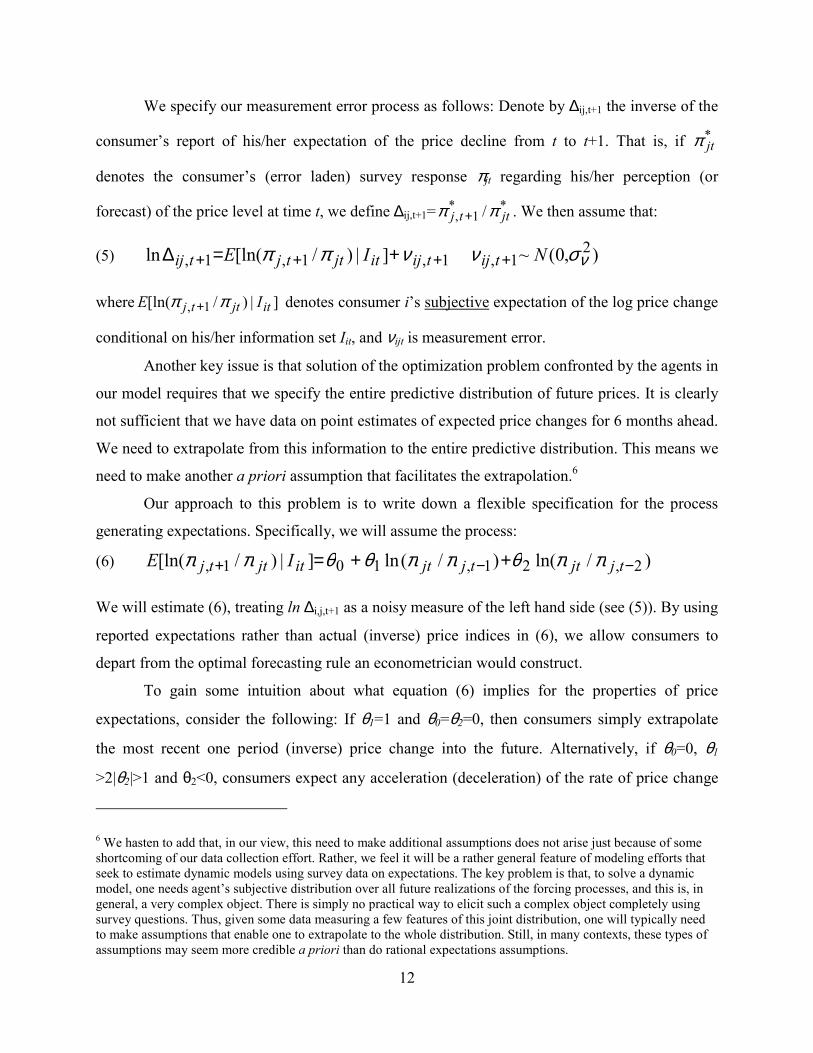
We specify our measurement error process as follows: Denote by ∆ij,t+1 the inverse of the

consumer’s report of his/her expectation of the price decline from t to t+1. That is, if *jtπ

denotes the consumer’s (error laden) survey response πjt regarding his/her perception (or

forecast) of the price level at time t, we define ∆ij,t+1= **1, / jttj ππ + . We then assume that:

(5) ),0(~]|)/[ln(ln 21,1,1,1, νσννππ NIE tijtijitjttjtij ++++ +=∆

where ]|)/[ln( 1, itjttj IE ππ + denotes consumer i’s subjective expectation of the log price change

conditional on his/her information set Iit, and νijt is measurement error.

Another key issue is that solution of the optimization problem confronted by the agents in

our model requires that we specify the entire predictive distribution of future prices. It is clearly

not sufficient that we have data on point estimates of expected price changes for 6 months ahead.

We need to extrapolate from this information to the entire predictive distribution. This means we

need to make another a priori assumption that facilitates the extrapolation.6

Our approach to this problem is to write down a flexible specification for the process

generating expectations. Specifically, we will assume the process:

(6) )/ln()/(ln]|)/ln([ 2,21,101, −−+ ++= tjjttjjtitjttj IE ππθππθθππ

We will estimate (6), treating ln ∆i,j,t+1 as a noisy measure of the left hand side (see (5)). By using

reported expectations rather than actual (inverse) price indices in (6), we allow consumers to

depart from the optimal forecasting rule an econometrician would construct.

To gain some intuition about what equation (6) implies for the properties of price

expectations, consider the following: If θ1=1 and θ0=θ2=0, then consumers simply extrapolate

the most recent one period (inverse) price change into the future. Alternatively, if θ0=0, θ1

>2|θ2|>1 and θ2<0, consumers expect any acceleration (deceleration) of the rate of price change

6 We hasten to add that, in our view, this need to make additional assumptions does not arise just because of some shortcoming of our data collection effort. Rather, we feel it will be a rather general feature of modeling efforts that seek to estimate dynamic models using survey data on expectations. The key problem is that, to solve a dynamic model, one needs agent’s subjective distribution over all future realizations of the forcing processes, and this is, in general, a very complex object. There is simply no practical way to elicit such a complex object completely using survey questions. Thus, given some data measuring a few features of this joint distribution, one will typically need to make assumptions that enable one to extrapolate to the whole distribution. Still, in many contexts, these types of assumptions may seem more credible a priori than do rational expectations assumptions.

13

that occurred from t-2 to t to continue into the future. If θ2<0 and |θ2|>|θ1+θ2|, consumers expect

mean reversion in the rate of price change towards the “natural rate”θ0/(1-θ1-2θ2). Given the

range of processes it can encompass, (6) is a fairly flexible model of expectation formation.

Using (6) we can construct estimates of consumers’ point expectations of price changes

from the current period to all future periods, ranging from 2 months ahead to the terminal period

of the planning problem, which we denote by T. For example, if the θ values in (6) are such that

consumers expect the rate of price decline to accelerate, we can calculate the extent to which the

expected rate of price decline over the next two months is less than that over the next six. Thus,

we can use (6) to construct E[lnπj,t+j/πjt|Iit] for j=1, …, T-t. Furthermore, E[lnπj,t+j|Iit] for any t+j

can be constructed from E[lnπj,t+j/πjt|Iit] because the current price levels πjt for j=IBM, Apple are

assumed to be elements of Iit.

Finally, note that having point estimates of a consumer’s price expectations at all time

horizons (out through T) is still not sufficient to solve the consumer’s dynamic choice problem.

We need to specify the subjective distribution of future prices at each horizon. For simplicity, we

will assume that agents’ subjective expectation of the distribution of prices at t+j is given by:

(7) ),]|[ln(~ln 2,, πσππ itjtjjtj IEN ++

where 2πσ is the subjective variance of the log price distribution. Unlike the θ ‘s in (6), 2

πσ is not

identified by the data on price perceptions/expectations, since we only have data on point

estimates and not measures of dispersion. It is identified in the complete structural model,

because it affects the option value of waiting and hence reservation prices.

III.3. Consumer Learning About Quality

The other key process we focus on in our model is that by which consumers learn about

the Qj - that is, the quality of the IBM/Compatible and Apple/Macintosh technologies. We

assume that consumers are Bayesians (although, as we discuss below, our estimation procedure

does not strictly impose this). They enter the market with priors on the Qj for j=IBM, Apple. We

assume that consumers have normal priors, given by:

(8) ),(~ 2jojoj QNQ σ

where Qj0 is the consumer’s prior expectation of the quality of computers of type j, and 2joσ is

the consumer’s prior uncertainty about computers of type j.

14

Consumers can learn about Qj, and thus reduce the variance 2joσ , by sampling from five

information sources, which we index by k. The five sources are: (1) retail stores, (2) articles in

computer specific publications, (3) articles in general-purpose publications, (4) advertisements,

and (5) word-of-mouth. Based on input from focus groups of recent PC buyers, managerial

interviews, and the literature reviewed in section II.1, we concluded these are the primary

information channels consumers use to gather information about PCs.7

In our model, these five information sources provide noisy signals of product quality.

Each source provides signals of different accuracy. Letting Sjkt denote a signal from source k at

time t about technology type j, the consumer knows that:

(9) ),(~ 2kjjkt QNS σ ,

where 1/ 2kσ is the precision of information contained in information source k, and Qj is the

“true” quality level of technology j=Apple/IBM. In estimation, we will allow for two different

types of consumers in regard to these true quality levels. Treating the consumer type as a latent

variable, we also estimate the population proportion of each type. However, in expositing the

model, we suppress the type specific subscript on the Qj for notational convenience.

At each time t, the consumer decides which set of information sources to visit. He/she

receives a quality signal from each visited source. The consumer then updates his/her quality

prior using standard Bayesian updating formulas. To write these formulas, it is convenient to

rewrite (9) as:

(9’) ),0(~ 2ktijktijktjjkt NxxQS σ+= .

and to recall equation (3), in which zijt denoted a consumer’s quality perception error for

technology j at time t:

(3’) ),0(~,]|[ 2ijtijtijtjitj NzzQIQE σ+= ,

where:

(10) }|])|[{( 22ititjijt IIQEQjE −=σ .

7 The data were collected from Sept. 1995 to June 1996. Panelists consistently ranked the Internet as one of the least important sources of information, so we do not include it. Since then, Internet usage has increased. However, many consumers, especially those looking for information on high-tech durables, seem to utilize the on-line versions of the same “core information channels,” such as reading Consumer Reports or magazine articles on-line. Thus, the Internet can be viewed as an alternative medium (electronic) to obtain information from each channel.

15

Then, letting Likt be a dummy variable indicating whether consumer i visits information source k

at time t, and assuming the signals are independent, we obtain the Bayesian updating formulas:

(11)

1

1

5

1 220

2 1−

= =

∑ ∑+=t

s k k

iks

jijt

Lσσ

σ

(12) )( 1,,5

1 221,,

21,,

1,, −= −

−− −∑

++= tjiijkt

k ktji

tjiikttjiijt zxLzz

σσ

σ

Equation (11) gives the evolution of the accuracy of the perception errors, whereas equation (12)

describes how perception errors themselves are updated given the quality signals. The

consumer’s subjective quality distribution for technology j at time t is then:

(13) )],|[(~ 2ijtitjj IQENQ σ .

Note that the perception errors zijt retain a normal distribution throughout the updating process.

One mechanism generating positive duration dependence in the purchase hazard is that

2ijtσ will fall over time as more information is acquired. From (4), we see that this increases

expected utility conditional on making a PC purchase. This suggests the following intuitive

argument for identification of the precisions 1/ 2kσ for k=1,5: If an information source is more

(less) accurate, the perception error variance 2ijtσ will fall more (less) after that source is visited.

This, in turn, is reflected in the extent to which the purchase hazard rises after a source is visited.

The use of stated preference data provides us with an additional source of information to

help identify the precisions. The basic idea is that, if an information source is very inaccurate,

then consumers will be very unlikely to update their quality perception substantially after visiting

that source. This is because the Kalman gain coefficient )/( 221,

21, ktijtij σσσ +−− associated with

that source in equation (12) will tend to be small. Thus, survey measures of how consumers’

quality perceptions evolve over time should help to identify the precisions. Furthermore, as we

argued earlier, the extent that perceived quality ratings change over time should help identify the

extent of prior uncertainty captured by the parameters 2joσ .

In each survey wave, we asked consumers to rate each technology on 7-point Likert

scales. More details on the questions will be provided in section VI. At this point, it suffices to

16

say that we treat responses to these perceived quality questions as providing measures of the

consumer’s underlying subjective quality perceptions E[Qj | Iit ] for j=IBM, Apple.

Specifically, we divide reported quality into a low, medium or high range. Denote these

as L, M and H, respectively. Let qijt denote consumer i’s reported quality perceptions at time t.

We assume these survey responses are generated by a quantal response model where:

jLitjijt IQEifLq µ≤= ]|[ ,

jHitjjLijt IQEifMq µµ <<= ]|[ ,

jHitjijt IQEifHq µ≥= ]|[ .

The µ’s are threshold parameters to be estimated. Of course, the E[Qj | Iit ] are random variables

from the perspective of the econometrician, because we observe only the number of signals a

consumer has received from each source, not their actual content. According to equation (3’), the

E[Qj | Iit ] are normally distributed with variance 2ijtσ . Thus, we obtain the ordered probit model:

)()Pr( jjLijtijt QLq −Φ== µσ ,

(14) )()()Pr( jjLijtjjHijtijt QQMq −Φ−−Φ== µµ σσ ,

)(1)Pr( jjHijtijt QHq −Φ−== µσ ,

where ijtσΦ is the normal distribution function with the mean 0 and variance 2

ijtσ . The response

probabilities in (14) will contribute to the likelihood function we construct in section V.8

Finally, we note that that our estimation procedure does not actually impose that

consumers update in a strict Bayesian manner. El-Gamal and Grether (1995), in their experiment

on Bayesian learning, found that, while Bayes’ rule was the most commonly used rule, subjects

often used a “representativeness heuristic.” This means they update too much when they receive

new information. Since we do not observe precisions of the information sources in our data, the

estimated precisions are free to depart from their “true” values. Increasing the estimated

precisions above their true values leads to behavior that is observationally equivalent to

excessive updating. Whether consumers are strictly Bayesian is not identified in our framework.

8 Note: In (14) we could have added an additional source of measurement error, so that consumer responses would be random even conditional on a known E[Qj | Iit ]. But we suspected that this would have little effect on the results.

17

IV. The Consumer’s Dynamic Optimization Problem

The state of a consumer at each point in the choice process is characterized by the

information set Iit introduced in the previous section. To be precise, Iit contains the complete set

of signals received by consumer i up through period t, which we denote by itx~ , for which the

subjective mean and variances of quality are sufficient statistics. It also contains the current and

lagged inverse price indices, and the consumer’s observed characteristics and latent type. That is:

(15) },,},,],~|[{{ ,1,2 τππσ iAppleIBMjtjjtijtitjit XxQEI =−= .

where Xi is a vector of consumer characteristics and τ=1,2 denote the latent type (see section

II.1). Note that ]~|[ itj xQE =E[Qj | Iit].

The consumer’s choice set at time t includes 25=32 combinations of the five potential

information sources that he/she may choose to utilize. After deciding which information sources

to sample, and seeing the resultant signals, the consumer can decide either to buy a computer or

wait until the next period. If the consumer decides to buy, there are 2⋅R possible choices (2

technologies and R expenditure levels). If the consumer decides to wait, he/she will face the

same choices at t+1. The value of each of the 32 options for information acquisition is:

(16) imtitN

ititP

itkkmk

itimt mIVmIVEcJIV ξ++Σ−==

)},(),,({max)(5

1 m=1,32

Here, the ck for k=1,5 denote the costs of obtaining information from each source k, which we

treat as parameters to be estimated. Jkm is an indicator for whether source k is included in

combination m. ξimt is an iid stochastic shock to the cost of using search option m at time t.

In (16), VitP denotes the value of the purchase option. It is defined as follows:

(17) ],|[max),(},{

mIUEmIV itijrtrj

itP

it =

This is the maximum over all possible technology and expenditure options {j=IBM, Apple,

r=1,R} of the expected utilities of those choices. These expected utilities were given in (4). The

expectations in (17) are conditional on the start of period information set Iit as augmented by

signals obtained from choosing search option m. The augmented state is denoted by (Iit, m). The

consumer does not know what signals will be obtained if search option m is chosen, so he/she

must take an expectation over the possible signals. The expectation operator in (16) incorporates

this integration over the distribution of the signals that may be received under search option m.

18

Finally NitV in (16) denotes the value of making no purchase at time t. This is:

(18) tititimm

iitN

it IVEUmIV 01,1,0 ][max),( εδ ++= ++

Thus, if no purchase is made at t, the consumer gets the per-period utility flow denoted by

U0(Xi)=γ0 + iXγ~ , where Xi is a vector of individual characteristics. Then at t+1, he/she will

repeat the process of deciding which information sources to visit, followed by the decision

whether or not to buy. The parameter δ is the discount rate. We discuss the contents of the Xi

vector in detail below. Here we note that it includes an indicator for whether the consumer

already has a home computer. Obviously this may be an important determinant of the flow utility

under the no-purchase option. The stochastic term εi0t can be interpreted as a shock to the value

of the no purchase option at time t, known to consumer i but unobserved by the econometrician.

The expectation in (18) is taken over realizations of the price indices πj,t+1 at time t+1.

Given (πj,t-1 , πj,t )∈ Iit, the consumer forms a subjective distribution over πj,t+1 using (6) and (7).

At t+1, the consumer will face the same choice over the m=1,32 search options, except that

he/she will have the augmented information set Iit+1 generated by Iit plus the information

received from the search option chosen at time t, plus the actual realization of πj,t+1.

Together, (16), (17) and (18) give the Bellman equations for the consumer’s dynamic

optimization (DP) problem. In order to solve the DP problem, we specify a finite terminal period

T and then construct the period specific value functions using backward recursion in the usual

way. We assume that if a consumer still does not buy in the terminal period T, then he/she

receives the discounted value of the per-period utility stream )(0 iXU over an infinite horizon.

Given that we have 6 waves of data covering roughly 10 months, we decided to specify a

terminal period of T=12, which corresponds to a 20-month planning horizon. As we’ll see, the

model predicts that the large majority of consumer will have bought a computer within 12

periods, so, not surprisingly, changing the terminal period seems to have little effect on our

results.

Finally, we note that, since the four state variables in (15) that characterize the evolution

of quality perceptions and prices are continuous, it is not possible to solve the DP problem

exactly. We use the Keane and Wolpin (1994) approach, which involves solving for the value

functions on a grid of state points and then extrapolating to the remaining points.

19

V. Consumer Choice Probabilities and the Construction of the Likelihood Function

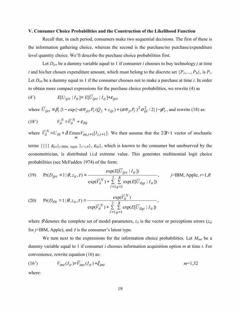
Recall that, in each period, consumers make two sequential decisions. The first of these is

the information gathering choice, whereas the second is the purchase/no purchase/expenditure

level quantity choice. We’ll describe the purchase choice probabilities first.

Let Dijrt be a dummy variable equal to 1 if consumer i chooses to buy technology j at time

t and his/her chosen expenditure amount, which must belong to the discrete set {P1,…, PR}, is Pr.

Let Di0t be a dummy equal to 1 if the consumer chooses not to make a purchase at time t. In order

to obtain more compact expressions for the purchase choice probabilities, we rewrite (4) as

(4’) ijrtitijrtitijrt IUEIUE ε+= ]|[]|[

where rijtrjtijtjrjrtiijrt PPzQPU γσαπαπβ −++−−≡ }}2/)()(exp{1{ 22 , and rewrite (18) as:

(18’) tiN

itN

it VV 0ε+=

where ][max 1,1,0 +++= titimm

iN

it IVEUV δ . We then assume that the 2⋅R+1 vector of stochastic

terms {{{{ εijrt}j=IBM, Apple }r=1,R}, εi0t}, which is known to the consumer but unobserved by the

econometrician, is distributed i.i.d extreme value. This generates multinomial logit choice

probabilities (see McFadden 1974) of the form:

(19) ∑ ∑+

==

= =

2

1 1)]|[exp()exp(

)]|[exp(),,|1Pr(

l

R

qitilqt

Nit

itijrtitijrt

IUEV

IUEzD τθ , j=IBM, Apple, r=1,R

(20) ∑ ∑+

==

= =

2

1 1

0)]|[exp()exp(

)exp(),,|1Pr(

l

R

qitilqt

Nit

Nit

ittiIUEV

VzD τθ ,

where θ denotes the complete set of model parameters, zit is the vector or perceptions errors (zijt

for j=IBM, Apple), and τ is the consumer’s latent type.

We turn next to the expressions for the information choice probabilities. Let Mimt be a

dummy variable equal to 1 if consumer i chooses information acquisition option m at time t. For

convenience, rewrite equation (16) as:

(16’) imtitimtitimt IVIV ξ+= )()( m=1,32

where:

20

)},(),,({max)(5

1mIVmIVEcJIV it

Nitit

Pitkkm

kitimt +Σ−=

=

We assume the vector of stochastic terms (ξi1t, …,ξi,,32,t), which is revealed to the consumer at

the start of period t, but which is unobserved by the econometrician, is distributed i.i.d extreme

value. This again generates multinomial logit choice probabilities of the form:

(21) ∑

==

=

− 32

1

1,))(exp(

))(exp(),,|1Pr(

litilt

itimttiimt

IV

IVzM τθ , m=1,32

Note that, by our timing conventions, zi,t-1 is the vector of quality perception errors at the start of

period t, prior to gathering any additional information.

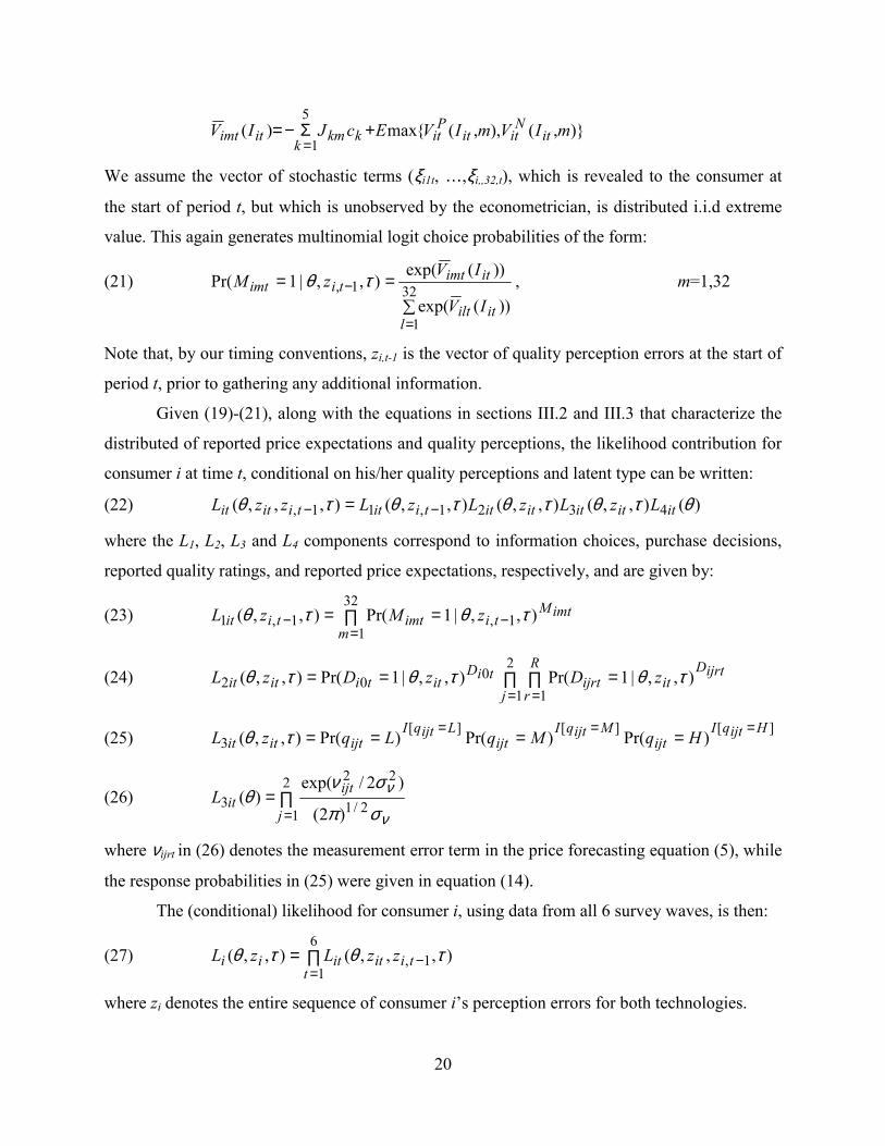
Given (19)-(21), along with the equations in sections III.2 and III.3 that characterize the

distributed of reported price expectations and quality perceptions, the likelihood contribution for

consumer i at time t, conditional on his/her quality perceptions and latent type can be written:

(22) )(),,(),,(),,(),,,( 4321,11, θτθτθτθτθ ititititittiittiitit LzLzLzLzzL −− =

where the L1, L2, L3 and L4 components correspond to information choices, purchase decisions,

reported quality ratings, and reported price expectations, respectively, and are given by:

(23) ∏ ===

−−32

11,1,1 ),,|1Pr(),,(

mimtM

tiimttiit zMzL τθτθ

(24) ∏ ∏ ==== =

2

1 1002 ),,|1Pr(),,|1Pr(),,(

j

R

r

ijrtDitijrttiD

ittiitit zDzDzL τθτθτθ

(25) ][][][3 )Pr()Pr()Pr(),,( HijtqI

ijtMijtqI

ijtLijtqI

ijtitit HqMqLqzL === ====τθ

(26) ∏==

2

1 2/1

22

3)2(

)2/exp()(

j

ijtitL

ν

ν

σπ

σνθ

where νijrt in (26) denotes the measurement error term in the price forecasting equation (5), while

the response probabilities in (25) were given in equation (14).

The (conditional) likelihood for consumer i, using data from all 6 survey waves, is then:

(27) ∏==

−6

11, ),,,(),,(

ttiititii zzLzL τθτθ

where zi denotes the entire sequence of consumer i’s perception errors for both technologies.

21

Since the econometrician does not observe either zi or τ, we must integrate them out as follows:

(28) ∑ ∫==

2

1)(),,()(

ττ τθλθ ii

iziii dzzfzLL

where λτ is the population type proportion of consumer type τ, and f(zi) denotes the joint density

of the perception errors. We know from section II.3 that f(zi) is a multivariate normal density,

with a rather complex intertemporal variance-covariance pattern governed by (11) and (12).

Unfortunately, zi is a 12-vector (there are 6 periods and two perception errors each period

– one for each technology) so the integral over zi in (28) is 12-dimensional. The evaluation of

such an integral by traditional methods is computationally impractical. Thus, we adopt the

simulated maximum likelihood (SML) approach, using 100 draws from the zi distribution to

simulate the integral (see, e.g., Lerman and Manski (1981), Pakes (1987), McFadden (1989),

Keane (1993)). This simulator is smooth, so a gradient-based method can be used to maximize

the simulated log-likelihood function. We used the Quasi-Newton method with line search. In

conjunction with this method, the BHHH algorithm is employed to approximate the Hessian.

VI. The Survey Data

In order to estimate the proposed model, we sought to construct a representative sample

of consumers throughout the U.S. who were in the market for a personal computer. Potential

panel members were first contacted in September 1995 by telephone using random digit dialing.

They were invited to participate in the panel if they met the following criteria: 1) they stated they

were extremely or very likely to buy a PC for their home within the next six to eight months, 2)

they were the member of the household most responsible for making the purchasing decision,

and 3) they were planning to spend more than $1,200 dollars on a computer. Of 7,733 contacted

individuals, 345 passed the screening process and were invited to participate in the panel.

The duration of our survey was based on prior information concerning the time that a

typical consumer spends making a PC purchase decision. Marketing managers at the PC

manufacturer we were working with estimated the purchase cycle for a personal computer to be

on average six months. Thus, in an attempt to capture the entire process for the majority of our

panel, we decided to collect data over a period of nine months.

Starting in October 1995 and ending in June 1996, panel members were asked to

complete six surveys, approximately one every seven weeks. To reduce attrition we provided a

22

variety of incentives to retain panel members. Panelists were paid $5 dollars for each completed

survey. Of the 345 individuals who received the first wave survey, 300 responded. However, we

eliminated 19 individuals due to missing information, leaving a sample size of N=281.

Table 1 describes the socio-demographic characteristics of the sample. The panelists tend

to have a higher level of education (61% possess an undergraduate or graduate degree), and a

higher income level (80% reported annual income between $35,000 and $80,000), than the

average American. The panel members reported their levels of computer expertise as 34%

“novices,” 52% “intermediate abilities,” and 14% “experts.” Slightly less than half the sample

(45%) reported this was their first time purchasing a personal computer.

In each survey, respondents were asked about their search activity since the last survey,

and whether they had yet made a PC purchase. They were re-surveyed at 7-week intervals until

they report a purchase, at which point detailed information on the configuration, brand, and price

were obtained. Once a purchase is reported, data collection on the individual ceases.

The top panel of Table 4 shows choice distributions by wave. That is, it shows how many

panelists were interviewed in each wave, and, of these, how many purchased an IBM/compatible

or Apple PC in each wave. “Wave 1” refers to the October 1995 survey. Interestingly, there are

no purchases in this wave, suggesting that the panelists tended to be at a relatively early stage of

the search process when they were selected for the project. This is a good thing from our

perspective, since we would like to capture search from an early stage.9

“Wave 2” refers to the second survey that respondents completed roughly seven weeks

later.10 Note that, since no purchases were reported in wave 1, all 281 panelists were surveyed

again in wave 2 (with no attrition). Of these 281 panelists, 19 bought an IBM and 1 bought an

Apple PC during period covered by the second wave survey. In the absence of sample attrition,

there should therefore have been 261 panelists surveyed in wave 3. However, as we see in Table

4, only 245 responded, giving a 6% attrition rate in wave 3. Attrition rates in the subsequent

three waves were 10%, 9% and 17% respectively.

9 On the other hand, it must be admitted that, unlike the other waves, the initial survey was sent out only 3 to 4 weeks after panelists were selected (and then had to be returned within two weeks). This creates a bias towards not finding as many purchases in the first wave as in subsequent waves, since a respondent who had made a purchase 5 or 6 weeks prior to the first survey could have been screened out of the panel during the initial phone interview. 10 We say “roughly” because respondents were allowed to return the survey within a two-week window. A respondent who returned the survey immediately would tend to have had a shorter gap since the previous survey.

23

Overall, the statistics in Table 4 indicate that, of the 281 original panelists, 102 made no

purchase by the end of wave 6, while 98 had bought a PC, and 81 had left the sample due to

attrition. Thus, attrition affects 29% of the original panelists. Given that the project’s duration

was almost 10 months and that the survey required at least 15 minutes of the panelist’s time, we

view this is a relatively good retention rate. Comparing the characteristics of subjects who attrite

vs. those who stay in the sample in each wave, we do not find evidence of significant differences.

The second panel of Table 4 presents attrition-adjusted calculations of the number of

panelists making each choice in each wave. That is, we treat the purchase hazard presented on

the right-hand side of the top panel as given, and adjust the sample size in each wave for

attrition. These calculations imply that, in the absence of attrition, 119 out of the original 281

panelists would have made a purchase by the 6th wave survey. In other words, if the purchase

hazard was the same for those who attrite as for those who remained in the survey, 21 out of the

81 attritors would have made a purchase by the 6th wave. This calculation implies that 40% of

the respondents have made a purchase by wave 6, which is 10 months after the original survey.

This suggests that managers we interviewed may have underestimated typical search durations.

In each survey we asked panelists if, during the previous 7-week period, they had

gathered information about PCs through: (1) store visits, (2) articles in general publications, (3)

articles in computer publications, (4) advertising, and (5) word-of-mouth. Our questions were

phrased in such a way as to try to capture active search, as opposed to purely passive exposure to

signals. For example, regarding articles in general publications, we asked: “Have you spent any

time reading articles on computer information in newspapers, general purpose magazines or

consumer guides?” And, regarding advertising, we asked: “Have you spent any time reading

advertisements about computers in newspapers, computer magazines, general purpose

magazines, or viewing TV commercials?” Thus, we asked if respondents had actually spent time

reading articles or reading/viewing ads, as opposed to merely being casually exposed to them.

We also asked panelists about their quality perceptions for both the IBM compatible and

Apple technologies. To construct a measure of perceived quality, respondents were asked to rate

each technology on 7-point Likert disagree-to-agree scales for the following five items: 1) “will

meet my needs for a long time to come,” 2) “is user friendly,” 3) “is powerful,” 4) “has a large

number of software titles,” and 5) “all components operate together without any problems

(hardware, software, peripherals).” Factor analysis suggested that the five items measured a

24

unidimensional construct. Thus, we constructed an overall quality measure by averaging the five

items. We report the reliability of the quality construct, as measured by the Cronbach’s alpha, in

Table 2. The alpha coefficients imply a high level of reliability and a high level of internal

consistency for the items. This is consistent across technologies and waves of the panel.

Recall that we incorporate in the likelihood whether a consumer reports a “low,”

“medium” or “high” quality level for each technology in each period (see equation (14)). Taking

our 7-point quality scale, we classified values in the [1-3), [3, 5] and (5,7] intervals as low,

medium, and high, respectively.

Finally, we also needed to collect data on actual and expected prices. We have already

described the construction of the price expectation data at some length in section III.2, so we will

not repeat that here. We will instead describe how we constructed the actual realized price

indices for each technology in each period. Recall that the (inverse) price indices πjt for j=IBM,

Apple that we need to construct are normalized to 1.0 at t=1 (i.e., in the first wave). Thus, we

need to construct measures of how prices changed from each wave to the next.

In order to measure how PC prices moved over the sample period, we first looked at the

PC configurations that panelists reported they were considering in the first wave. We matched

these with retail prices obtained from industry data to measure their prices. We then chose 5

representative configurations that cost approximately $1500, $2000, $2500, $3000 and $3500 in

October 1995, one each for IBM and Apple. Next, we used industry data to examine how prices

of each configuration moved over the sample period. Using a sales weighted average of the

configuration prices, our calculations implied that prices fell approximately 10% from October

1995 through June 1996. This translates into a 15% annual rate, which is quite close to the 16%

annual rate that consumers expected on average.

A 15% price decline may seem small, but it is important to note that this refers to the

price of an entire configuration, not just the CPU. According to National Income and Product

Account (NIPA) data, PC prices fell by 31% from 1995 to 1996, but the price of terminals was

flat, while that of storage devices fell only 13%, and that of other peripheral equipment fell 22%.

The NIPA data also show that price declines for PCs, monitors, memory and other peripheral

equipment accelerated substantially beginning in 1997, after our sample period had ended.

The five discrete dollar amounts noted above were also what we assumed as the elements

of agents’ discrete consumption choice set {P1, …, PR} in solving and estimating the model.

25

VII. Empirical Results

VII.1. Parameter Estimates

Table 3 reports the simulated maximum likelihood estimates of our model parameters.

We start by discussing the price expectation process parameters. To facilitate interpretation it is

useful to rewrite equation (6) in terms of prices (rather than the inverse price indices):

)/ln()/(ln]|)/ln([ 2,21,101, −−+ ++−= tjjttjjtitjttj PPPPIPPE θθθ

)/ln()/(ln)( 2,1,21,210 −−− +++−= tjtjtjjt PPPP θθθθ

Our estimate of θ0 is 0.041. Thus, if price were constant from t-2 to t (zeroing out the 2nd and 3rd

terms), consumers would expect a 4.1% price decline from t to t+1 (i.e., over the next 2 months).

Since our estimate of θ2 is negative and larger in absolute value than θ1+θ2, our estimated

expectations process implies that consumers expect mean reversion in price changes. The

process implies a steady state expected rate of price decline of 2.5% per two-month period. Since

consumers expect mean reversion, if prices had declined at a rate that was greater (less) than

2.5% from t-2 to t, then consumers would expect a price decline of less (more) than 2.5% over

the next two months. The expectations process implies a 16% annualized rate of expected price

decline, which is similar to what actually occurred (see section VI).

The estimate of the standard deviation of measurement error for reported price change

expectations (i.e., the σν in equation (5)) is 0.088, implying substantial measurement error in

consumers’ reports of their own expectations. Our estimate of the perceived standard deviation

of future price changes around consumers’ point expectations (i.e., the σπ in equation (6)) is

0.076. Thus, consumers perceive substantial volatility in price changes around their means.

Next we discuss the parameters that determine expected utility conditional on purchase

(see eqn. (4)). The price coefficient is statistically significant and positive, implying the

conditional indirect utility function is decreasing in price, as we would expect. The estimates of

the equation for the utility weight parameter, ii Xβββ ~0 += , indicate that consumers get more

utility from home computer capabilities if they are: 1) more experienced with computers, 2)

older, 3) less educated,11 and 4) male. The effect of income on the utility weight is statistically

11 The age variable was entered as Age/35. The education variable ranged from 0 to 6 (for the seven ascending categories listed in Table 1). This was entered as education/6, giving a variable ranging from 0 to 1.

26

insignificant. That more educated people get less marginal utility from additional home computer

capability may reflect the fact that they are more likely to have access to computers at work.

The parameter α was normalized to 1.0 (without loss of generality) for identification.

Note that we cannot identify α, the scale of the quality variables Qj, and the scales of the prior

and signal standard deviations, at the same time. For instance, one could double α while halving

the Qj, halving the prior standard deviations σj0, and halving all the signal standard deviations σk.

This would halve the σijt in (4), and leave expected utility unchanged. Since we resolve this

identification problem by normalizing α, the extent of risk aversion is subsumed in the scale of

the quality measures and the scale of the prior and signal standard deviations. This does not alter

the behavioral implications of the model.

We also had to normalize the constant term in the βi equation. While technically

identified, the likelihood was quite flat over a range of values for this parameter and the same set

of quality level and quality variance parameters discussed above. A first order Taylor series

expansion of the utility function in (2) around Q=0 gives U(Q) ≈ πPβQ - γP + ε. This suggests

that it may be difficult to distinguish the scale of β from the scale of the Q’s, which is indeed

what we find. Thus, we normalized β0 =1.

The equation for the No-purchase utility implies, as one would expect, that the No-

purchase utility is higher for individuals who already own a computer. Furthermore, older

people, women and lower income people have a higher No-purchase utility than younger people,

men and higher income people. Education and experience do not have a statistically significant

effect on No-Purchase utility.

We turn next to the estimates of the quality of each technology. Recall that we allow for

two latent types of consumers in terms of their match quality with each technology. Our

estimates imply that consumers who belong to the first latent segment perceive a higher match

quality for the IBM compatible technology, while type 2 consumers prefer the Apple technology.

However, the first segment constitutes 88% of the population, implying that the majority of

consumers feel that IBM/compatibles serve their needs better than Apple technology.

The prior standard deviation of quality perceptions is statistically significant, and very

large relative to the true quality levels of the two technologies. This indicates that there is

substantial prior quality uncertainty in this market. Note that the prior uncertainty for Apple is

27

larger than for IBM. Since the Windows platform is more widely used than the Apple platform,

consumers presumably have more prior exposure to information about IBM compatibles.

Table 3 also reports the estimated characteristics of each of the five information sources.

The estimates imply that store visits provide the most precise information. Word-of-mouth is the

next most accurate information source. Articles in computer magazines, articles in general

publications, and advertising provide the noisiest information.12

In regard to costs associated with information sources, the estimates imply that store

visits are the most costly way to gather information. The least costly method is word-of-mouth.

Interestingly, reading articles in computer magazines is estimated to be quite a bit more costly

than reading computer articles in general publications, or reading ads.

VII.2. Model Fit

Table 4 provides evidence on how the model fits the data on purchase decisions. The top

panel of the table describes the data itself. It reports the sample proportion of consumers who

make each choice (No-purchase, IBM, Apple) in each 7-week period (or “wave”). The second

panel provides attrition adjusted estimates of the choice frequencies, as discussed in section IV.

The bottom panel of Table 4 reports simulated choice frequencies based on our estimated

model. We simulated choice paths for 2000 hypothetical consumers, and then re-based the

statistics from this simulation to an initial sample size of N=281 (for comparability with the

observed data). We refer to the bottom panel of Table 4 as the “baseline” simulation of the

model. We extend the simulation for 12 waves, which corresponds to roughly 12⋅7=84 weeks, or

about 20 months. Since the data used in estimation extend for only 6 waves, the first 6 waves of

the simulation are an in-sample forecast, while the last 6 waves are an out-of-sample forecast.

To see how the model fits the data, one needs to compare the middle and bottom panels

of Table 4. The model fits most of the broad features of the data rather well. After 6 waves, or

roughly 10 months, the model predicts that 39.9% of consumers would have bought an IBM (or

IBM compatible) computer, while 1.9% would have bought an Apple. The corresponding figures

in the data are 40.2% and 2.1%, respectively.

12 During the estimation process, we decided to set the precisions for advertising, general sources and computer sources to be equal. We were having numerical difficulties in trying to pin down all three of these terms separately, and we could not reject a specification where these three channels had equal signaling variances.

28

A striking feature of the data is the clear positive duration dependence in the purchase

hazard. The no-purchase frequency declines almost monotonically from 100% in wave 1, to

92.9% in wave 2, …, to 89.5% in wave 5, and to 85% in wave 6. The model captures this overall

pattern rather well. For instance, it predicts a no-purchase rate of 93.0% in wave 2, falling

gradually to 89.7% in wave 5, and these figures are very close to the actuals.

The model predicts that 5.7% of consumers buy in wave 1, whereas, as we discussed in

section IV, no survey respondents reported buying during the first wave.13 Of course, any model

with a significant stochastic component to choice behavior would likely have difficult generating

such an extreme outcome in a particular period. In addition, the model somewhat overstates the

no-purchase rate in wave 6 (89.2% vs. 85% in the data). Thus, the model somewhat understates

the degree of positive duration dependence that we see in the data. However, given sampling

error in the sample purchase frequencies, the discrepancies do not appear to be serious.14

Table 5 provides evidence on how the model fits the data on search behavior. The layout

of this table is just like Table 4, except that the choices now are whether or not to utilize each of

the 5 information sources in each wave. Again, the model fits the broad features of the data

reasonably well. The model slightly underpredicts the extent of search. For instance, it predicts

that, over the first 6 waves, households visit a store in 36.2% of the periods, whereas in the data

the frequency of store visits is 40.1%. This pattern of under-predicting the utilization rate by

about 3 or 4 percentage points holds across all five information sources.

The model accurately predicts the relative utilization of each information source. The

most widely used source is word-of-mouth (66.5% utilization in the data vs. 62.1% in the

model), while the least utilized source is articles in computer magazines (38.9% utilization in the

data, vs. 35% in the model). Of course, these utilization differences are generated by the

differential costs and precisions of the information sources, as estimated in Table 3.15

13 As we discussed earlier, the first wave survey came only a few weeks after the screening interview, so any consumer who bought 5 to 7 weeks before the first survey would have been screened from the data set. This would have biased downward the number of purchases in wave 1, but we abstracted from this in setting up our model. 14 The standard error on the 85% sample frequency for wave 6 is 2.6%. 15 An interesting question is how the model can distinguish if one information source is less utilized than another because it is more expensive or less accurate (or some combination of both). The distinction would obviously not be identified (absent strong functional form assumptions) using data on information source utilization alone. However, our estimation brings two additional sources of information to bear: purchase decisions and stated quality ratings. If an information source is more accurate than another, quality ratings will be more likely to move, and perceived risk of a brand will be more likely to fall (implying a greater increase in the purchase hazard), after that source is visited.

29

Another striking feature of the data is negative duration dependence search intensity. For

instance, the percentage of consumers who gather information via store visits drops from 64.4%

in wave 1 to 29.2% in wave 6. The model predicts a decline from 60.5% to 25.5%. Thus, aside

from the tendency to under-predict utilization by a few percent in each period, the model

captures the time path of utilization very well. The same is true for all five information channels.

One reason for search intensity to fall over time is that the marginal value of search tends

to fall as consumers acquire more information. This is a direct consequence of the Bayesian

variance updating formula (equation 11), which implies that each additional signal has a smaller

variance reducing effect. That is, if Nk denotes the number of signals received from source k,

then 242 // kkN σσσ −=∂∂ , and this is decreasing in Nk since σ 4 is decreasing in Nk.

But this can’t be the whole story, because this intuition is purely static. In a dynamic

setting, negative duration dependence in search intensity seems to contradict the flavor of results

in Moscarini and Smith (2001), to the effect that search should be concentrated into the period

just prior to making a decision. Basically, if one discounts the future, it doesn’t make sense to

engage in costly search today, and then delay a decision for several periods. But two factors alter

this logic in the present context: price fluctuations and taste shocks. Intuitively, in our model, it

makes sense to acquire good information about brand attributes quickly, enabling one to form a

clear idea of which brand one prefers. One may then delay purchase until one sees a good price

for the preferred brand, or until one receives a good positive taste shock.

Of course, an alternative explanation for negative duration dependence in search intensity

is a compositional effect. Specifically, those consumers who search less intensely may stay in the

market longer. However, this story does not seem consistent with the data. Fixed effects logit

models for whether a consumer utilizes an information source in each wave show negative time

effects, similar in magnitude to the patterns in Table 5. Compositional effects are not important

in the model either. We only allowed for unobserved heterogeneity in consumer preferences for

Apple vs. IBM, and negative duration dependence is present for each type separately.

VIII. Counterfactual Experiments

In this section we present a number of counterfactual experiments designed to clarify the

nature of consumer behavior implied by the model. These experiments are all based on simulated

choice histories for 2000 hypothetical agents. These agents are presented with the same random

draws for the stochastic terms of the model as were the 2000 hypothetical agents used in the

30

baseline simulation reported in the bottom panels of Tables 4 and 5. Thus, any differences in

choice behavior between the experimental treatments and the baseline model simulation will be

due entirely to differences in the economic environment.

VIII.1. Effects of Expected Price Declines and Learning on Purchase Delay

The first set of experiments is designed to examine the roles of expected price declines

vs. learning in generating purchase delay. The top panel of Table 6 presents a simulation where,

in each wave t, consumers assume that the mean of the price distribution will remain at the

present level for all future periods. That is, we modify equation 7 so that, at time t, consumers’

subjective expectation of the distribution of future prices is given by:

ln πj,t+k ∼ N(ln πjt|σπ2) for j=IBM, Apple, k=1,2,…,T

where πjt is the current price index. Note that consumers still expect prices to fluctuate over time,

according to the variance σπ2, but they no longer expect a downward trend in prices. Another

way to describe this experiment is that we set θ0 = θ1 = θ2 in equation 6.

According to the top panel of Table 6, taking away the expectation of a downward trend

in prices results in acceleration of purchases. The purchase hazard shifts up in the first 6 periods,

stays about the same in periods 7-9, and shifts down in periods 10-12. The percentage of

consumers predicted to buy by the end of wave 6 increases from 41.8% (see Table 4) to 46.3%.

But the percentage of consumers who are predicted to buy by the end of wave 12 remains almost

unchanged (81.6% vs. 81.9%). Note, however, that positive duration dependence in the purchase

hazard remains strong even under this counterfactual experiment. Thus, most of the positive

duration dependence in the hazard does not appear to be due to the expectation of falling prices.

We don’t find this relatively small effect of expected price declines on purchase timing

surprising for two reasons. First, as we noted earlier, another factor inducing positive duration

dependence in the purchase hazard is simply that prices do fall over time, a factor that would be

present even in a static model. Second, learning is another source of duration dependence.

The bottom panel of Table 6 reports the results of an experiment designed to evaluate the

role of learning in generating purchase delay. In this experiment, we implement a substantial

increase in the cost of search. Specifically, we increase the cost visiting all five information

sources by 60%. Making learning more expensive leads to a noticeable flattening of the purchase

hazard. While the hazard rises from 5.7% in wave one to 20.1% in wave 12 under the baseline

(an increase by a factor of 3.5), the increase under the experiment is from 5.2% to 14.4% (a

31

factor of only 2.8). Making learning more expensive also shifts the purchase hazard downward,

leading to lower computer sales overall. The percentage of consumers who buy by the end of 6

waves is predicted to decline from 41.8% (see the bottom panel of Table 4) to 38.5%, while the

percentage predicted to buy by the end of wave 12 drops from 81.6% to 73.7%.

Conversely, a reduction in search costs, which leads to more search, accentuates the

positive duration dependence in the purchase hazard. Thus, our results imply that both expected

price declines and the desire to gather information both contribute to purchase delay.

VIII.2. How Price Expectations Affect Price Elasticities of Demand

In this section we present two experiments designed to examine how price expectations

affect demand elasticities. Recall that our estimates of consumers’ subjective price expectation

process imply that consumers expect a steady state rate of price decline of roughly 2.5% per two-

month period, and that they expect mean reversion in price declines. Thus, if price were to fall by

some much larger amount in a particular wave, consumers would expect a price rebound in the

following wave. This should augment the demand response to the price cut. In Table 7 we report

two experiments designed to evaluate the magnitude of this type of effect.

In the top panel of Table 7, we simulate the effect of a 20% transitory price cut for both

IBM and Apple in wave 2, holding prices fixed in all other waves. In this experiment, consumers

are assumed to form expectations according to our estimates of their subjective price

expectations process. As a result, since the 20% price decline in wave 2 is so unusually large,

consumers expect a price rebound in wave 3. Our estimates imply that the price cut induces the

percentage of consumers who buy in wave 2 to increase from 7.0% (baseline model) to 11.7%.

This is a 67% increase in sales, implying a short run price elasticity of demand with respect to a

transitory price cut of roughly 3.4.

In the bottom panel of Table 7, we report the results of an experiment in which prices are

cut by 20% in wave 2, but expectations are held fixed. That is, consumers’ expectations of the

price decline from wave 2 to waves 3, 4, …, T are held fixed at their pre-experimental levels. In

other words, consumers view the dramatic price decline in wave 2 as a one time structural break

in the price process, which will have no bearing on future price changes. Our estimates imply

that this type of price cut induces the percentage of consumers who buy in wave 2 to increase

from 7.0% to 10.2%. This 46% increase in sales implies a short run price elasticity of demand

with respect to a transitory price cut, holding expectations fixed, of roughly 2.3.

32

Thus, our results imply that expectations play a major role in how consumers respond to a

price change. The elasticity of demand with respect to a transitory price cut is nearly 50% greater

if we incorporate how the price cut alters consumers’ expectations of future price changes than if

we hold those expectations fixed (i.e., 3.4 vs. 2.3). This suggests that static models may

potentially give rather misleading estimates of price elasticities of demand. It also suggests that

estimates of demand elasticities in dynamic models could be quite sensitive to our assumptions

about expectations, thus highlighting the importance of collecting subjective expectations data.

Another issue that the simulations in Table 7 address is the extent to which a temporary

price cut leads to purchase acceleration vs. incremental sales. That is, to what extent does the

price cut simply cannibalize future sales? Comparing the baseline simulation (Table 4) with the

experiment (Table 7), we see that the price cut induces 12.4 additional consumers to buy in wave

2. Looking further out, we see that 117.3 consumers buy a PC by the end of wave 6 in the

baseline, compared to 127.3 in the experiment, an increase of 10.0.16 Thus, by wave 6, 10.0 out

of 12.4, or 80%, of the additional period 2 sales induced by the price cut represent incremental

sales, while only 20% represent cannibalization of sales from waves 3 through 6.

This story changes if we extend the analysis through to the terminal period (wave 12).

229.3 consumers buy a PC by the end of wave 12 in the baseline, compared to 233.9 in the

experiment, an increase of 4.6. Thus, by wave 12, only 4.6 out of the extra 12.4 sales induced by

the wave 2 price cut (or 37%) represent incremental sales.

It is also interesting to note the asymmetric affects of the price cuts on IBM Compatible

vs. Apple sales. Under the baseline, the percentages of consumers predicted to buy IBM or Apple

PCs by the end of wave 6 are 39.9% and 1.9%, respectively. With the 20% price cut (for both

technologies) in wave 2, these figures increase to 42.7% and 2.6%. Thus, Apple sale increase

37% while IBM sales increase only 7%. This difference occurs in part because, in wave 2, Apple

sale increase 100% while IBM sales increase 65%. But, in addition, the cannibalization of future

sales is greater for IBM. In fact, the price cut slightly increases Apple sales in subsequent

periods. This stems from the learning dynamics in the model. The substantial price cut in wave 2

16 Recall that these figures are from a simulation of 2000 consumers, re-based to a population of N=281. That is why there are fractional numbers of consumers.

33

induces consumers to recognize it is a good period to buy. This encourages more search in period

2, so consumers learn more about Apple. Since prior uncertainty about Apple is greater, events

that encourage more learning tend to favor Apple. This is discussed further in the next section.

VIII.3. How the Cost and Accuracy of Information Sources Affect Choice Behavior

In this section we examine how altering the cost and accuracy of the various information

sources would alter choice behavior. Table 8 reports two experiments where search costs are

reduced. In the top panel we reduce the cost of store visits, the most costly and most accurate

information source, by 20%. This leads to an upward shift in the purchase hazard by roughly 1 to

2.5 points in all periods. In the baseline simulation (Table 4), 41.8% of consumers have bought

by the end of wave 6, while under the experiment this increases to 48.1%.

In the bottom panel, we reduce the cost of acquiring information through advertisements

by 20%. Operationally, this might involve a manufacturer making its ads more readable or more

easily accessible. This again leads to an acceleration of purchases, increasing the percentage of

consumers who buy by the end of wave 6 to 46.0%. The effect is smaller than for store visits

because reading advertisements is less expensive and provides less accurate information. Effects

of reducing the costs of acquiring information from articles in general publications, articles in

computer publications and word-of-mouth are similar, so we do not report them.

An interesting aspect of the experiments in Table 8 is that reducing the cost of acquiring

information has a much more positive effect on Apple sales than on IBM sales. For instance,

with a 20% decrease in the cost of acquiring information via a store visit, the percentage of

consumers who buy an IBM or IBM compatible by the end of wave 12 increases from 77.5% to

78.7%, while the percent that buy an Apple increases from 4.1% to 6.2% (a 50% increase).

However, the asymmetric positive effect for Apple is much less dramatic when we reduce the

cost of gathering information via advertisements (which increases Apple sales from 4.1% to

4.7%), and the same is true for the other three information channels (not reported). This is

presumably because these alternative channels are less costly and less accurate than store visits.

Table 9 reports a set of experiments where we increase the accuracy of the information

sources. This again leads to an upward shift in the purchase hazard. Increasing the precision of

information provided by store visits by 20% increases the percentage of consumers who buy by

the end of wave 6 from 41.8% (baseline) to 49.6%. The percentage of consumers who buy by the

end of wave 12 increases from 81.6% (baseline) to 85.3%. The effect on sales is again

34

proportionately much greater for Apple than for IBM, with Apple sales by the end of wave 12

rising from 4.1% to 7.0%. Results for the other information sources are similar.

Thus, we find that making information more freely available, either by lowering the cost

or increasing the accuracy of signals, favors the Apple platform. This occurs because consumers

have much greater prior uncertainty with respect to the match quality of the Apple platform.

IX. Conclusion

We have estimated a dynamic model of how consumers learn about and choose between

different brands of PCs, with an emphasis on the choice between the IBM Compatible and

Apple/Macintosh technologies. Our work extends recent work on estimation of Bayesian

learning models of consumer choice behavior in environments characterized by uncertainty

about brand attributes. Specifically, while several authors have estimated models of passive

learning about brand attributes, we estimate a model of active learning – i.e., a model in which

consumers make optimal sequential decisions about how much information to gather prior to

making a purchase.

Our work also makes two methodological contributions. Following the suggestion of

Manski (2003), we collected data on consumer price expectations and used these data to model

consumers’ price expectation process. To our knowledge, this is the first time that a dynamic

structural model has been estimated using such an approach in lieu of the typical rational

expectations assumption.17 Also, following the suggestion of McFadden (1989a), we incorporate

stated brand quality information into our likelihood function, rather than modeling only revealed

preference data (i.e., data on purchases and observed search behavior).

Our analysis has shed light on how consumer choice behavior is influenced by both

forward-looking price expectations and the process of learning about quality. A key finding is

that estimates of dynamic price elasticities of demand – i.e., demand elasticities that account for

how a price change today alters expectations of future price changes – exceed estimates that

ignore the expectations effect by roughly 50%.

17 There has been prior work using data on expectations to predict choice behavior in choice models that are static, or that can be interpreted as reduced form approximations to the optimal decision rules from dynamic models. Examples include Delevande (2003), who models how expected effectiveness of different birth control methods affects choice of method, and Lochner (2003), who models how expected apprehension probabilities affect decisions to engage in criminal activity.

35

This occurs because our estimated expectations formation process implies that consumers

expect mean reversion in price changes. That is, if there is an exceptionally large price cut today,

consumers expect a price rebound tomorrow. This enhances the incentive to buy now.

Our findings highlight the more general point that estimates of demand elasticities from

static models, or estimates from dynamic models that make incorrect expectational assumptions,

can be quite misleading. To the extent that demand elasticities are sensitive to how consumers

form price expectations, it becomes important to collect data on expectations to learn more about

how they are formed.

Finally, while our work has focused specifically on the PC market and on the choice

between Apple and IBM compatible technologies, the modeling approach we develop here

should be useful for studying a wide range of high-tech, high-involvement durable goods

markets where active learning about different technologies is important.

36

REFERENCES Ackerberg, D. (2003): “Advertising, Learning, and Consumer Choice in Experience Good Markets:

A Structural Empirical Examination,” International Economic Review, 44, 1007-1040. Anand, Bharat, and Ron Shachar (2002): "Risk Aversion and Apparently Persuasive Advertising."

Harvard Business School Working Paper Series, No. 02-099. Beatty, Sharon E. and Scott M. Smith (1987): “External Search Effort: An Investigation across

Several Product Categories,” Journal of Consumer Research, 14, 83-95. Bridges, Eileen, Chi Kin Yim, and Richard A. Briesch (1995): “A High-Tech Product Market Share

Model with Customer Expectations,” Marketing Science, 14, 61-81. Bridges, Eileen, Anne T. Coughlan and Shlomo Kalish (1991): “New Technology Adoption in an

Innovative Marketplace: Micro- and Macro-Level Decision Making Models,” International Journal of Forecasting, 7, 257-270.

Brucks, Merrie (1985): “The Effects of Product Class Knowledge on Information Search Behavior,”

Journal of Consumer Research, 12, 1-16. Ching, Andrew (2002): “Consumer Learning and Heterogeneity: Dynamics of Demand for

Prescription Drugs After Patent Expiration,” Working Paper, Ohio State University. Claxton, John D., Joseph N. Fry and Bernard Portis (1974): “A Taxonomy of Prepurchase

Information Gathering Patterns,” Journal of Consumer Research, 1, 35-43. Crawford, Gregory S. & Shum, Matthew (2003): "Uncertainty and Learning in Pharmaceutical

Demand: Anti-Ulcer Drugs," Working Paper, University of Arizona. Delevande, Adeline (2003): “Pill, Patch or Shot? Subjective Expectations and Birth Control Choice,”

Working Paper, Northwestern University. Eckstein, Zvi, Dan Horsky and Yoel Raban (1988): “An Empirical Dynamic model of Brand

Choice,” Working Paper No. 88, University of Rochester. El-Gamal, M. A. and D. M. Grether (1995): “Are People Bayesian? Uncovering Behavioral

Strategies,” Journal of the American Statistical Association, 90, 1137−1145. Erdem, Tülin and Michael P. Keane (1996): "Decision-Making under Uncertainty: Capturing

Dynamic Brand Choice Processes in Turbulent Consumer Goods Markets," Marketing Science, 15, 1-20.

Erdem, Tülin, Susumu Imai and Michael P. Keane (2003): “Brand and Quantity Choice

Dynamics under Price Uncertainty,” Quantitative Marketing and Economics, 1, 5-64. Furse, David H., Girish N. Punj and David E. Stewart (1984): "A Typology of Individual Search

Strategies Among Purchases of New Automobiles," Journal of Consumer Research, 10, 417-431.

37

Glazer, Rashi (1991): "Marketing in an Information-Intensive Environment: Strategic Implications of Knowledge as an Asset," Journal of Marketing, 55, 1-19.

Glazer, Rashi and Allen M. Weiss (1991): "Marketing in Turbulent Environments: Decision

Processes and the Time-Value of Information," Working Paper No. 1145, Graduate School of Business, Stanford University.

Gönül, Füsun and Kannan Srinivasan (1996): “Estimating the Impact of Consumer

Expectations of Coupons on Purchase Behavior: A Dynamic Structural Model,” Marketing Science, 15, 262-279.

Harris, Katherine and Michael P. Keane (1999): “A Model of Health Plan Choice: Inferring

Preferences and Perceptions from a Combination of Revealed Preference and Attitudinal Data,” Journal of Econometrics, 89, 131-157.

Hauser, John R, Glen L. Urban, and Bruce D. Weinberg (1993): “How Consumers Allocate Their

Time when Searching for Information,” Journal of Marketing Research, 30, 452-467. Hendel, Igal and Aviv Nevo (2002): “Measuring the Implications of Sales and Consumer Stockpiling

Behavior,” Working Paper, UC Berkeley. Holak, Susan L., Donald R. Lehmann and Fareena Sultan (1987): “The Role of Expectations in the

Adoption of Innovative Consumer Durables: Some Preliminary Evidence,” Journal of Retailing, 63, 243-259.

Keane, Michael P. (1993): "Simulation Estimation for Panel Data Models with Limited Dependent

Variables," in G.S. Maddala, C.R. Rao and H.D. Vinod (Eds.), Handbook of Statistics, Elsevier Science Publishers.

Keane, Michael P. and Kenneth Wolpin (1994): “Solution and Estimation of Dynamic Programming

Models by Simulation,” Review of Economics and Statistics, 76, 648-672.

Kiel, Geoffrey C. and Roger A. Layton (1981): "Dimensions of Consumer Information Seeking," Journal of Consumer Research, 8 233-239.

Krishna, Aradhna (1992): "The Normative Impact of Consumer Price Expectations,"

Marketing Science, 11, 359-371.

Lerman, Steven and Charles Manski (1981): "On the Use of Simulated Frequencies to Approximate Choice Probabilities,” in Structural Analysis of Discrete Data with Econometric Applications, eds. C. Manski and D. McFadden. Cambridge: MIT Press.

Lochner, Lance (2003): “Individual Perceptions of the Criminal Justice System,” Working Paper,

University of Western Ontario. Manski, Charles F. (2003): "Inference on Expectations and Decisions," Econometrica,

forthcoming.

38

McFadden, Daniel (1974): "Conditional Logit Analysis of Qualitative Choice Behavior," in Frontiers of Econometrics, P. Zarembka, ed. New York: Academic Press, 105-42.

McFadden, Daniel (1989a): "The Choice Theory Approach to Market Research," Marketing Science,

5, 275-297. McFadden, Daniel (1989b): "A Method of Simulated Moments for Estimation of Discrete

Response Models without Numerical Integration," Econometrica, 57, 995-1026. Melnikov, Oleg (2000): “Demand for Differentiated Durable Products: The Case of the

US Computer Printer market,” Working Paper, Yale University. Meyer, Robert and Joao Assuncao (1990): "The Optimality of Consumer Stockpiling

Strategies," Marketing Science, 9, 18-41.

Moorthy, Sridhar, Brain T. Ratchford and Debabrata Talukdar (1997): "Consumer Information Search Revisited: Theory and Empirical Analysis," Journal of Consumer Research, 23, 263-277.

Moscarini, Giuseppe and Lones Smith (2001), “The Optimal Level of Experimentation,”

Econometrica, 69, 1629-1644. Newman, Joseph and Richard E. Staelin (1973): "Information Sources of Durable Goods," Journal of

Advertising Research, 13, 19-29.

Pakes, Ariel (1987): Patents at Options: Some Estimates of Value of Holding European Patent Stocks, Econometrica, 57, 1027-1058.

Roberts, John H. and Glen L. Urban (1988): " Modeling Multiattribute Utility, Risk, and Belief

Dynamics for New Consumer Durable Brand Choice," Management Science, 34, 167-185. Song, Inseong and Pradeep Chintagunta (2003): “A Micromodel of New Product Adoption with

Heterogeneous and Forward-Looking Consumers: Application to the Digital Camera Category,” forthcoming in Quantitative Marketing and Economics.

Srinivasan, Narasimhan and Brain T. Ratchford (1991): "An Empirical Test of a Model of External

Search for Automobiles," Journal of Consumer Research, 18, 233-242.

Weiss, Allen M. and Jan B. Heide (1993): "The Nature of Organizational Search in High Technology Markets," Journal of Marketing Research, 30, 220-33.

Westbrook, Robert A. and Claes Fornell (1979): "Patterns of Information Source Usage Among

Durable Goods Buyers," Journal of Marketing Research, 16, 303-312. Urbany, Joel E., Peter R. Dickson and William L. Wilkie (1989): "Buyers’ Uncertainty and

Information Search," Journal of Consumer Research, 16, 208-215. Van der Klaauw, Wilbert and Kenneth I. Wolpin (2003): “Social Security, Pensions and the Savings

Behavior of Households.” Working Paper, University of North Carolina.

39

TABLE 2

Quality of Technology: Coefficient Alpha

Wave 1 Wave 2 Wave 3 Wave 4 Wave 5 Wave 6

IBM/Compatible .76 .80 .79 .83 .81 .80

Apple/Macintosh .79 .80 .82 .84 .83 .80

TABLE 1 Summary Statistics

Education % Income % Age %

Elementary school through 6th 0 Under $20,000 3.6 Under 18 7Junior high school (7-8) 1.0 $20,000 to $34,999 13 18 - 24 4High School (9-12) 13.7 $35,000 to $49,999 27 25 - 34 24Trade or vocational school 3.3 $50,000 to $64,999 24 35 - 44 34Some college 21.4 $65,000 to $79,999 14 45 - 54 23Undergraduate degree 34.1 $80,000 to $99,999 6 55 - 64 7Graduate School (Ph.D. or Masters)

26.4 $100,000 or over 13 65 or over 2

Expertise % Past Purchase % Gender %Novice 34 First time buyer 45 Male 62Intermediate 52 Female 38Expert 14

No Purchase Utility Coefficientsθ 0 0.041 (0.012) Constant 3.917 (1.258)

θ 1 1.239 (0.163) Ownership of Computer 0.149 (0.061) θ 2 -0.958 (0.194) Experience 0.009 (0.049) σ ν 0.088 (0.013) Age 0.644 (0.278)

Education -0.019 (0.089) Gender 0.543 (0.245)

σ π 0.076 (0.043) Income -0.294 (0.124)

Information Search Process Parameters

Price Coefficent 0.478 (0.193) Prior Std.Dev. of Quality PerceptionIBM 0.927 (0.160)

1.000 - Apple 2.071 (0.350)

0.995 - Variability of Information

Store Visit 1.977 (0.659) Ads and Articles 4.741 (1.976)

Constant 1.000 - Word of Mouth 3.128 (1.325) Experience 0.479 (0.238) Age 0.207 (0.103) Information CostsEducation -0.734 (0.257) Store Visits 1.415 (0.123) Gender 0.639 (0.283) General Articles 0.642 (0.088) Income -0.670 (0.399) Computer Articles 1.137 (0.175)

Advertising 0.379 (0.052) Quality Coefficients Word of Mouth 0.318 (0.057)

Mean Quality( IBM)a 0.891 (0.397) Mean Quality( Apple)a -0.891 -Mean Quality( IBM)b -0.275 (0.125) IBM-Left -1.741 (0.267) Mean Quality( Apple)b 0.275 - IBM-Right 2.867 (0.419)

Apple-Left -3.217 (0.569) Apple-Right 2.433 (0.388)

1st Latent Class 0.879 (0.155) 2nd Latent Class 0.121 -

a 1st Latent Classb 2nd Latent Class

Note. Values enclosed in parentheses represent standard errors.

Latent Class Probabilities

Discount Factor

Quality Perception Interval Coefficients

TABLE 3 Parameter Estimates

Price Process Parameters

Utility Parameters

Utility Parameters (continued)

Price Process Coefficents

Measurement Error Std. Dev.

Utility Weight

Risk Aversion Coefficient

Table

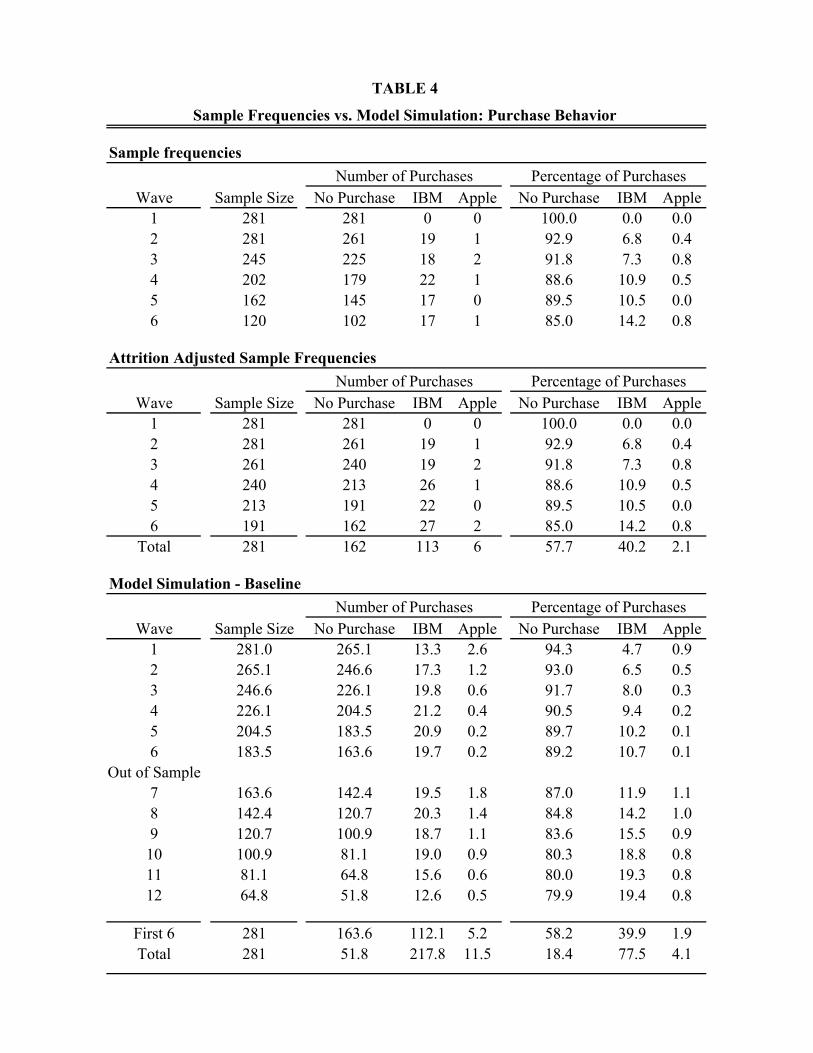
Wave Sample Size No Purchase IBM Apple No Purchase IBM Apple1 281 281 0 0 100.0 0.0 0.02 281 261 19 1 92.9 6.8 0.43 245 225 18 2 91.8 7.3 0.84 202 179 22 1 88.6 10.9 0.55 162 145 17 0 89.5 10.5 0.06 120 102 17 1 85.0 14.2 0.8

Wave Sample Size No Purchase IBM Apple No Purchase IBM Apple1 281 281 0 0 100.0 0.0 0.02 281 261 19 1 92.9 6.8 0.43 261 240 19 2 91.8 7.3 0.84 240 213 26 1 88.6 10.9 0.55 213 191 22 0 89.5 10.5 0.06 191 162 27 2 85.0 14.2 0.8

Total 281 162 113 6 57.7 40.2 2.1

Wave Sample Size No Purchase IBM Apple No Purchase IBM Apple1 281.0 265.1 13.3 2.6 94.3 4.7 0.92 265.1 246.6 17.3 1.2 93.0 6.5 0.53 246.6 226.1 19.8 0.6 91.7 8.0 0.34 226.1 204.5 21.2 0.4 90.5 9.4 0.25 204.5 183.5 20.9 0.2 89.7 10.2 0.16 183.5 163.6 19.7 0.2 89.2 10.7 0.1

Out of Sample7 163.6 142.4 19.5 1.8 87.0 11.9 1.18 142.4 120.7 20.3 1.4 84.8 14.2 1.09 120.7 100.9 18.7 1.1 83.6 15.5 0.910 100.9 81.1 19.0 0.9 80.3 18.8 0.811 81.1 64.8 15.6 0.6 80.0 19.3 0.812 64.8 51.8 12.6 0.5 79.9 19.4 0.8

First 6 281 163.6 112.1 5.2 58.2 39.9 1.9Total 281 51.8 217.8 11.5 18.4 77.5 4.1

TABLE 4

Sample Frequencies vs. Model Simulation: Purchase Behavior

Sample frequenciesNumber of Purchases Percentage of Purchases

Number of Purchases Percentage of Purchases

Attrition Adjusted Sample FrequenciesNumber of Purchases Percentage of Purchases

Model Simulation - Baseline

Sample Frequencies

Wave Sample SizeStore Visits

General Articles

Computer Articles Advertising

Word of Mouth

Store Visits

General Articles

Computer Articles Advertising

Word of Mouth

1 281 181 164 148 188 247 64.4 58.4 52.7 66.9 87.92 281 115 116 98 163 204 40.9 41.3 34.9 58.0 72.63 245 82 101 87 132 136 33.5 41.2 35.5 53.9 55.54 202 77 87 83 121 116 38.1 43.1 41.1 59.9 57.45 162 46 64 53 77 94 28.4 39.5 32.7 47.5 58.06 120 35 50 41 59 76 29.2 41.7 34.2 49.2 63.3

Wave Sample SizeStore Visits

General Articles

Computer Articles Advertising

Word of Mouth

Store Visits

General Articles

Computer Articles Advertising

Word of Mouth

1 281 181 164 148 188 247 64.4 58.4 52.7 66.9 87.92 281 115 116 98 163 204 40.9 41.3 34.9 58.0 72.63 261 87 107 92 140 144 33.5 41.2 35.5 53.9 55.54 240 91 103 98 143 137 38.1 43.1 41.1 59.9 57.45 213 60 84 69 101 123 28.4 39.5 32.7 47.5 58.06 191 55 79 65 93 120 29.2 41.7 34.2 49.2 63.3

Total 1467 589 653 570 828 975 40.1 44.5 38.9 56.4 66.5

Model Simulation - Baseline

Wave Sample SizeStore Visits

General Articles

Computer Articles Advertising

Word of Mouth

Store Visits

General Articles

Computer Articles Advertising

Word of Mouth

1 281 170 164 139 189 231 60.5 58.4 49.5 67.3 82.22 265 88 103 81 155 179 33.2 38.9 30.6 58.5 67.53 247 71 92 83 129 126 28.7 37.2 33.6 52.2 51.04 226 83 84 78 125 123 36.7 37.2 34.5 55.3 54.45 205 51 72 57 89 106 24.9 35.1 27.8 43.4 51.76 184 47 65 55 81 109 25.5 35.3 29.9 44.0 59.2

Out of Sample7 164 42 59 46 70 98 25.6 36.0 28.0 42.7 59.88 143 35 47 40 58 76 24.5 32.9 28.0 40.6 53.19 122 29 39 34 46 62 23.8 32.0 27.9 37.7 50.8

10 102 24 36 27 41 50 23.5 35.3 26.5 40.2 49.011 82 19 27 23 31 40 23.2 32.9 28.0 37.8 48.812 65 16 21 19 26 32 24.6 32.3 29.2 40.0 49.2

First 6 1408 510 580 493 768 874 36.2 41.2 35.0 54.5 62.1Total 2086 675 809 682 1040 1232 32.4 38.8 32.7 49.9 59.1

TABLE 5Sample Frequencies vs. Model Simulation: Search Behavior

Number of Consumers Collecting Information Percentage of Consumers Collecting Information

Attrition Adjusted Sample Frequencies

Number of Consumers Collecting Information Percentage of Consumers Collecting Information

Number of Consumers Collecting Information Percentage of Consumers Collecting Information

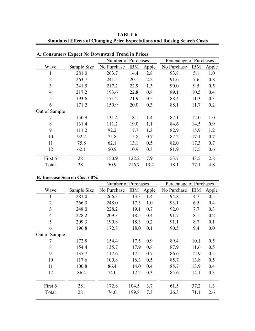
Wave Sample Size No Purchase IBM Apple No Purchase IBM Apple1 281.0 263.7 14.4 2.8 93.8 5.1 1.02 263.7 241.5 20.1 2.2 91.6 7.6 0.83 241.5 217.2 22.9 1.3 90.0 9.5 0.54 217.2 193.6 22.8 0.8 89.1 10.5 0.45 193.6 171.2 21.9 0.5 88.4 11.3 0.36 171.2 150.9 20.0 0.3 88.1 11.7 0.2

Out of Sample7 150.9 131.4 18.1 1.4 87.1 12.0 1.08 131.4 111.2 19.0 1.1 84.6 14.5 0.99 111.2 92.2 17.7 1.3 82.9 15.9 1.210 92.2 75.8 15.8 0.7 82.2 17.1 0.711 75.8 62.1 13.1 0.5 82.0 17.3 0.712 62.1 50.9 10.9 0.3 81.9 17.5 0.6

First 6 281 150.9 122.2 7.9 53.7 43.5 2.8Total 281 50.9 216.7 13.4 18.1 77.1 4.8

Wave Sample Size No Purchase IBM Apple No Purchase IBM Apple1 281.0 266.3 13.3 1.4 94.8 4.7 0.52 266.3 248.0 17.3 1.0 93.1 6.5 0.43 248.0 228.2 19.1 0.7 92.0 7.7 0.34 228.2 209.3 18.5 0.4 91.7 8.1 0.25 209.3 190.8 18.3 0.2 91.1 8.7 0.16 190.8 172.8 18.0 0.1 90.5 9.4 0.0

Out of Sample7 172.8 154.4 17.5 0.9 89.4 10.1 0.58 154.4 135.7 17.9 0.8 87.9 11.6 0.59 135.7 117.6 17.5 0.7 86.6 12.9 0.510 117.6 100.8 16.3 0.5 85.7 13.8 0.511 100.8 86.4 14.0 0.4 85.7 13.9 0.412 86.4 74.0 12.2 0.3 85.6 14.1 0.3

First 6 281 172.8 104.5 3.7 61.5 37.2 1.3Total 281 74.0 199.8 7.3 26.3 71.1 2.6

TABLE 6

B. Increase Search Cost 60%Number of Purchases Percentage of Purchases

Simulated Effects of Changing Price Expectations and Raising Search Costs

A. Consumers Expect No Downward Trend in PricesNumber of Purchases Percentage of Purchases

Wave Sample Size No Purchase IBM Apple No Purchase IBM Apple1 281.0 265.1 13.3 2.6 94.3 4.7 0.92 265.1 234.2 28.4 2.5 88.3 10.7 1.03 234.2 214.4 18.8 1.0 91.6 8.0 0.44 214.4 192.8 21.1 0.6 89.9 9.8 0.35 192.8 172.6 19.8 0.4 89.5 10.3 0.26 172.6 153.7 18.7 0.2 89.1 10.8 0.1

Out of Sample7 153.7 133.4 18.5 1.8 86.8 12.0 1.28 133.4 112.8 19.3 1.4 84.5 14.4 1.19 112.8 93.9 17.8 1.1 83.2 15.8 1.010 93.9 75.0 18.1 0.8 79.9 19.2 0.911 75.0 59.5 14.9 0.6 79.4 19.8 0.812 59.5 47.1 11.9 0.5 79.1 20.1 0.8

First 6 281 153.7 120.0 7.3 54.7 42.7 2.6Total 281 47.1 220.4 13.5 16.8 78.4 4.8

Wave Sample Size No Purchase IBM Apple No Purchase IBM Apple1 281.0 265.1 13.3 2.6 94.3 4.7 0.92 265.1 237.9 25.1 2.0 89.8 9.5 0.83 237.9 218.2 19.1 0.6 91.7 8.0 0.34 218.2 197.0 20.7 0.6 90.3 9.5 0.35 197.0 176.7 20.1 0.2 89.7 10.2 0.16 176.7 157.5 19.0 0.2 89.2 10.7 0.1

Out of Sample7 157.5 137.1 18.8 1.7 87.0 11.9 1.18 137.1 116.2 19.6 1.3 84.8 14.3 1.09 116.2 97.1 18.1 1.0 83.5 15.6 0.910 97.1 77.9 18.3 0.8 80.3 18.9 0.911 77.9 62.2 15.1 0.6 79.8 19.4 0.812 62.2 49.6 12.1 0.5 79.7 19.5 0.8

First 6 281 157.5 117.3 6.2 56.1 41.7 2.2Total 281 49.6 219.2 12.2 17.6 78.0 4.3

Number of Purchases Percentage of Purchases

A. 20% Price Decline in Wave 2 - Total EffectNumber of Purchases Percentage of Purchases

TABLE 7Price Cut Simulations

B. 20% Price Decline in Wave 2 - Expected Future Price Changes Held Fixed

Wave Sample Size No Purchase IBM Apple No Purchase IBM Apple1 281.0 258.1 18.2 4.7 91.8 6.5 1.72 258.1 233.9 21.4 2.7 90.6 8.3 1.03 233.9 209.6 22.7 1.6 89.6 9.7 0.74 209.6 187.4 21.3 1.0 89.4 10.1 0.55 187.4 165.6 21.2 0.6 88.4 11.3 0.36 165.6 145.8 19.3 0.5 88.1 11.7 0.3

Out of Sample7 145.8 125.1 18.9 1.9 85.8 12.9 1.38 125.1 104.8 18.8 1.5 83.8 15.0 1.29 104.8 86.1 17.5 1.2 82.1 16.7 1.110 86.1 68.8 16.4 0.9 79.9 19.0 1.111 68.8 54.6 13.6 0.7 79.3 19.7 1.012 54.6 42.4 11.7 0.4 77.7 21.5 0.8

First 6 281 145.8 124.1 11.0 51.9 44.2 3.9Total 281 42.4 221.0 17.6 15.1 78.7 6.2

Wave Sample Size No Purchase IBM Apple No Purchase IBM Apple1 281.0 261.4 15.6 3.9 93.0 5.6 1.42 261.4 239.5 20.1 1.8 91.6 7.7 0.73 239.5 216.2 22.4 0.9 90.3 9.4 0.44 216.2 194.5 21.1 0.5 90.0 9.8 0.25 194.5 172.2 22.0 0.3 88.5 11.3 0.26 172.2 151.8 20.2 0.2 88.1 11.7 0.1

Out of Sample7 151.8 130.8 19.4 1.6 86.1 12.8 1.18 130.8 110.0 19.5 1.3 84.1 14.9 1.09 110.0 91.5 17.6 1.0 83.1 16.0 0.910 91.5 73.5 17.2 0.8 80.3 18.8 0.811 73.5 58.9 14.0 0.6 80.2 19.0 0.812 58.9 47.3 11.2 0.4 80.3 19.0 0.7

First 6 281 151.8 121.5 7.7 54.0 43.2 2.7Total 281 47.3 220.4 13.3 16.8 78.4 4.7

TABLE 8

B. 20% Decrease in the Cost of Gathering Information from AdvertisingNumber of Purchases Percentage of Purchases

Simulated Effects of Decreasing Search Costs

A. 20% Decrease in the Cost of a Store VisitNumber of Purchases Percentage of Purchases

Wave Sample Size No Purchase IBM Apple No Purchase IBM Apple1 281.0 256.7 18.7 5.6 91.4 6.6 2.02 256.7 231.5 21.7 3.5 90.2 8.5 1.43 231.5 206.9 22.9 1.7 89.4 9.9 0.74 206.9 183.3 22.6 1.0 88.6 10.9 0.55 183.3 161.4 21.2 0.7 88.1 11.5 0.46 161.4 141.7 19.2 0.5 87.8 11.9 0.3

Out of Sample7 141.7 121.1 18.7 1.9 85.4 13.2 1.38 121.1 101.0 18.6 1.5 83.4 15.3 1.29 101.0 83.3 16.5 1.2 82.5 16.4 1.210 83.3 66.2 16.1 0.9 79.5 19.4 1.111 66.2 52.4 13.2 0.7 79.1 19.9 1.012 52.4 41.4 10.6 0.4 79.0 20.2 0.8

First 6 281 141.7 126.2 13.1 50.4 44.9 4.7Total 281 41.4 219.9 19.7 14.7 78.3 7.0

Wave Sample Size No Purchase IBM Apple No Purchase IBM Apple1 281.0 256.3 18.0 6.7 91.2 6.4 2.42 256.3 230.2 22.5 3.6 89.8 8.8 1.43 230.2 204.3 24.2 1.7 88.7 10.5 0.74 204.3 179.4 23.9 1.0 87.8 11.7 0.55 179.4 156.7 22.0 0.6 87.4 12.3 0.36 156.7 136.5 19.8 0.4 87.1 12.6 0.3

Out of Sample7 136.5 116.3 18.5 1.7 85.2 13.6 1.28 116.3 96.8 18.2 1.3 83.3 15.6 1.19 96.8 78.6 17.2 1.0 81.2 17.7 1.110 78.6 62.3 15.6 0.8 79.2 19.8 1.011 62.3 49.2 12.5 0.6 79.0 20.1 0.912 49.2 38.2 10.5 0.5 77.6 21.4 1.1

First 6 281 136.5 130.5 14.0 48.6 46.4 5.0Total 281 38.2 222.9 19.9 13.6 79.3 7.1

Wave Sample Size No Purchase IBM Apple No Purchase IBM Apple1 281.0 261.3 15.2 4.5 93.0 5.4 1.62 261.3 235.4 23.5 2.5 90.1 9.0 1.03 235.4 209.9 24.4 1.1 89.2 10.4 0.54 209.9 185.8 23.5 0.6 88.5 11.2 0.35 185.8 163.1 22.3 0.4 87.8 12.0 0.26 163.1 142.3 20.6 0.2 87.2 12.6 0.1

Out of Sample7 142.3 121.5 19.3 1.5 85.4 13.6 1.08 121.5 101.5 18.9 1.1 83.5 15.5 0.99 101.5 84.0 16.6 0.9 82.7 16.4 0.910 84.0 68.1 15.3 0.7 81.0 18.2 0.811 68.1 55.0 12.5 0.5 80.8 18.4 0.712 55.0 44.6 10.0 0.4 81.1 18.2 0.7

First 6 281 142.3 129.5 9.2 50.6 46.1 3.3Total 281 44.6 222.1 14.3 15.9 79.0 5.1

Number of Purchases Percentage of Purchases

TABLE 9

Number of Purchases Percentage of Purchases

B. Advertising, Articles in General and Computer Publications - 20% Increase in PrecisionNumber of Purchases Percentage of Purchases

C. Word-of-Mouth - 20% Increase in Precision

Simulated Effects of Making Information Sources More Accurate

A. Store Visit - 20% Increase in Precision