remote sensing

Article

Learning a Transferable Change Rule from a RecurrentNeural Network for Land Cover Change Detection

Haobo Lyu 1,†, Hui Lu 1,2,* and Lichao Mou 3,4,†

1 The Ministry of Education Key Laboratory for Earth System Modeling, Center for Earth System Science,Tsinghua University, Beijing 100084, China; lvhb15@mails.tsinghua.edu.cn

2 The Joint Center for Global Change Studies, Beijing 100875, China3 Remote Sensing Technology Institute (IMF), German Aerospace Center (DLR), Wessling 82234, Germany;

lichao.mou@dlr.de4 Signal Processing in Earth Observation (SiPEO), Technical University of Munich (TUM),

Munich 80333, Germany* Correspondence: luhui@tsinghua.edu.cn; Tel.: +86-10-6277-2565; Fax.: +86-10-6279-7284† These authors contributed equally to this work.

Academic Editors: Petri Pellikka, Lars Eklundh, Heiko Balzter, Lars T. Waser and Prasad S. ThenkabailReceived: 3 March 2016; Accepted: 12 June 2016; Published: 16 June 2016

Abstract: When exploited in remote sensing analysis, a reliable change rule with transfer abilitycan detect changes accurately and be applied widely. However, in practice, the complexity of landcover changes makes it difficult to use only one change rule or change feature learned from a givenmulti-temporal dataset to detect any other new target images without applying other learningprocesses. In this study, we consider the design of an efficient change rule having transferabilityto detect both binary and multi-class changes. The proposed method relies on an improved LongShort-Term Memory (LSTM) model to acquire and record the change information of long-termsequence remote sensing data. In particular, a core memory cell is utilized to learn the change rulefrom the information concerning binary changes or multi-class changes. Three gates are utilizedto control the input, output and update of the LSTM model for optimization. In addition, thelearned rule can be applied to detect changes and transfer the change rule from one learned image toanother new target multi-temporal image. In this study, binary experiments, transfer experimentsand multi-class change experiments are exploited to demonstrate the superiority of our method.Three contributions of this work can be summarized as follows: (1) the proposed method can learnan effective change rule to provide reliable change information for multi-temporal images; (2) thelearned change rule has good transferability for detecting changes in new target images withoutany extra learning process, and the new target images should have a multi-spectral distributionsimilar to that of the training images; and (3) to the authors’ best knowledge, this is the first timethat deep learning in recurrent neural networks is exploited for change detection. In addition, underthe framework of the proposed method, changes can be detected under both binary detection andmulti-class change detection.

Keywords: change detection; LSTM model; transferability; multi-spectral image; recurrent neural network

1. Introduction

With the development of remote sensing, the dynamic observation of the Earth has led to a greatdeal of available, detailed, accurate and up-to-date change information for use in learning about andmonitoring our planet [1]. Change detection is important for detecting dynamic changes of the Earth.Change detection attempts to identify land cover differences in the same geographical area acrossa period of time [2] and can be applied to various domains, including urban expansion [3], disaster

Remote Sens. 2016, 8, 506; doi:10.3390/rs8060506 www.mdpi.com/journal/remotesensing

Remote Sens. 2016, 8, 506 2 of 22

monitoring [4], land cover map updating [5], forest degradation survey [6] and glacier melting [7].In this context, various types of multi-temporal images are exploited to resolve the above problems.Among them, multi-spectral data with sufficient spectra and fine spatial resolution provide a powerfulability to detect changes.

In the literature, many algorithms have been designed for detecting changes, each with differentadvantages. Generally, these methods can be divided into four categories as follows:

(1) Image algebra: To detect changes directly, image differencing and image ratios are widely used todetect changes between multi-temporal images. Among them, image differencing (subtractionrule) is a robust and efficient method for detecting changes, and Change Vector Analysis (CVA) [8]represents its conceptual extension with an integrated theoretical framework, therein providinggood performance.

(2) Post-classification: Changed objects are acquired from independent classified multi-temporalmaps, and land cover changes can be easily identified from the separately-classified maps.Therefore, numerous classification methods [9,10] have been proposed to improve changedetection accuracy. In particular, a novel change-detection-driven transfer learning approach [11]was proposed to update land cover maps via the classification of image time series.

(3) Feature learning and transformation: In this category, new learned (transformed) or selectedfeatures are utilized to distinguish changes, especially using a distance metric. Amongthe change feature learning methods, physically-meaningful features and learned changefeatures both lead to a good performance and have been applied in various domains. Asphysically-meaningful features, vegetation indices, forest canopy variables and water indices areoften extracted to identify changes in specific ground-object types [12,13]. For learned featuresand transformations, various features or transformed feature spaces are learned to highlight thechange information to detect a changed region more easily than when using the original spectralinformation of multi-temporal images, such as in Principal Component Analysis (PCA) [14],Multivariate Alteration Detection (MAD) [15], subspace learning [16,17], sparse learning [18] andslow features [19].

(4) Other advanced methods: Change detection can be formulated as a statistical hypothesis testusing physical models [20]. The metric learning method [21] is also an effective method ofdetecting changes using well-learned distances. In addition, canonical correlation analysis [22,23]and clustering methods [24,25] have been proposed and found to perform well in unsupervisedchange detection tasks.

The above change detection methods all achieve good performances and make variouscontributions. However, limitations also exist and should be resolved to better detect changes. Formulti-spectral images, all available spectral bands should be considered effectively to detect changes.Moreover, the learned change information should be recorded and exploited for sequential time seriesdata with transferability. In addition, an integrated and independent change detection method canbe exploited to detect changes more widely and conveniently without the supplementary task ofthreshold selection or classification at the final decision step.

To overcome the above limitations, we expect to design an integrated and independent changerule in our method to detect changes with all available spectral information, and the change rule canbe transferred to new target multi-temporal images. Briefly, the effective change rule should have areliable capability for change information representation, and the learned change rule can be transferredto new target images without any extra learning process, which demonstrates its transferability.In addition, in this paper, transferability is restricted to new target multi-temporal imageswhose spectral distributions are similar (the same number of spectral bands) to those of trainingmulti-temporal images. Recently, some researchers [11] have proposed a change-detection-driventransfer leaning approach for updating land cover maps using classification, which has emphasizedthe importance of transferability in change detection research. Therefore, it is important to design

Remote Sens. 2016, 8, 506 3 of 22

an integrated change rule for detecting changes directly with transfer capacity, where the transfercapacity relies on a reliable capability in terms of the expression of the change information extractionfor sequential time series data. A Recurrent Neural Network (RNN) can be used to achieve theabove objectives. RNNs [26] are network models that use recurrent connections between their neuralactivations at consecutive time steps; such models use hidden layers or memory cells to learn thetime-evolving states that model the underlying dynamics of the input sequence for sequential timeseries data. RNN models have gained significant attention for solving many challenging problemsinvolving sequential time series data, especially Long Short-Term Memory (LSTM) models [27]. In anRNN learning framework, learning an appropriate representation of the sequences is an important stepfor achieving artificial intelligence. For change detection, it is important to have a reliable capability interms of the expression of change information extraction for detecting changes. Thus, RNN modelsrepresent potential approaches for learning reliable difference information and providing memorabilityfor change detection in sequential time series remote sensing data.

In this paper, we propose a new change detection method named REFEREE (learninga transferable change Rule From a recurrent neural network for change detection). The main idea ofthe proposed approach is learning an efficient change rule with a reliable capability in terms of theexpression of difference information extraction for detecting changes. For the process of learning areliable change rule, REFEREE provides transferability with a memory function to detect changes inan integrated change detection system. Therefore, REFEREE adapts LSTM models to resolve not onlybitemporal change problems, but also multi-class change detection problems (the definition can befound in Section 2). In addition, REFEREE is the first method that exploits the RNN framework to learna “change rule” for the change detection task on remote sensing images; moreover, a specially-designedLSTM model is tailored to represent the change information, which is not considered in traditionalRNN models, such as those in the literature [28,29].

The remainder of this paper is organized as follows. The experimental data and some definitionsconcerning multi-class changes in this study are described in Section 2. The details of our method arepresented in Section 3. The experimental setup for the parameters and the experimental design aredescribed in Section 4. The experimental results and discussion are presented in Section 5. Section 6concludes this paper.

2. Image Preparation

The performance of the proposed method is evaluated on three datasets. Among them,two multi-spectral datasets were acquired by the Landsat 7 Enhanced Thematic Mapper Plus (ETM+)sensor with six bands and a spatial resolution of 30 m. The last dataset was selected from imagesobtained by the EO-1 Hyperion, which is the first civil hyperspectral sensor on-board the EarthObserving One (EO-1) satellite and includes 242 spectral bands with a spatial resolution of 30 m. Withthe restricted condition of the spectral distributions in the transfer experiments (more details can befound in Section 4.3), only six bands, which are similar to the band range of the ETM sensor, wereselected from the EO-1 Hyperion images for evaluating the REFEREE model. Before using these data,the digital numbers (DNs) of the original data can be converted into absolute radiance (i.e., all ofthe datasets utilized in the experiments are normalized into a range of [0, 1]). Moreover, both theexperimental datasets and corresponding ground truth are acquired from the literature [19].

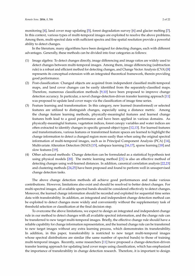
(1) Taizhou images: The first dataset consists of two images acquired for the city of Taizhou,China, in March 2000 (T1) and February 2003 (T2), with a WGS-84 projection and a coordinate range of31◦14’55.84 N–31◦27’39.26 N, 120◦02’24.38 E–121◦07’45.15 N. The two images are both 400× 400 pixels,and the two images show changes mainly related to city expansion, as shown in Figure 1a,b, in Bands 4,3 and 2. Figure 1c,d shows the labeled binary ground truth and multi-class ground truth, respectively.Here, the multi-class changes contain unchanged regions and three classes of changed regions: cityexpansion (bare soil, grassland or cultivated field to buildings or roads); changed soil (cultivated fieldto bare soil); and changed water areas (no-water regions to water regions). Additionally, the multi-class

Remote Sens. 2016, 8, 506 4 of 22

changes are changes such that the change types can be certain, although the classes at different timesteps are not certain. Taking city expansion as an example, the class characterizing one pixel may bebare soil, grassland or cultivated field at time T1, whereas the class of the same geographical pixelmay be a building or road at time T2. Then, we are unsure if the pixel changed from a certain class toanother label, whereas the change type of this pixel is certain to be city expansion. This is unsuitablefor traditional supervised classification-based change detection methods that learn change informationwithout land cover maps at different time steps.

（a） （b） （c） （d）

Figure 1. The pseudocolor images of Taizhou with RGB 432, acquired in (a) March 2000 and(b) February 2003. The labeled ground truth of the Taizhou images: (c) binary ground-truth, whereunchanged areas are shown in gray, changed areas are shown in white and black indicates an unlabeledregion not used for testing; (d) ground-truth of multi-class changes, where unchanged areas are shownin red, changed areas of city expansion are shown in green, changed soil areas are shown in orange,changed water areas are shown in blue and gray represents unlabeled regions (more details can befound in Section 4.3).

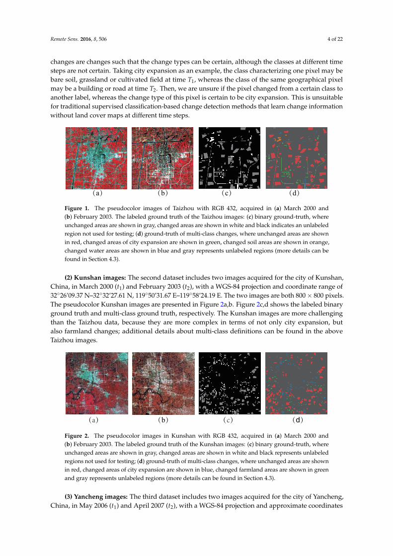
(2) Kunshan images: The second dataset includes two images acquired for the city of Kunshan,China, in March 2000 (t1) and February 2003 (t2), with a WGS-84 projection and coordinate range of32◦26’09.37 N–32◦32’27.61 N, 119◦50’31.67 E–119◦58’24.19 E. The two images are both 800× 800 pixels.The pseudocolor Kunshan images are presented in Figure 2a,b. Figure 2c,d shows the labeled binaryground truth and multi-class ground truth, respectively. The Kunshan images are more challengingthan the Taizhou data, because they are more complex in terms of not only city expansion, butalso farmland changes; additional details about multi-class definitions can be found in the aboveTaizhou images.

（a） （b） （c） （ ）

Figure 2. The pseudocolor images in Kunshan with RGB 432, acquired in (a) March 2000 and(b) February 2003. The labeled ground truth of the Kunshan images: (c) binary ground-truth, whereunchanged areas are shown in gray, changed areas are shown in white and black represents unlabeledregions not used for testing; (d) ground-truth of multi-class changes, where unchanged areas are shownin red, changed areas of city expansion are shown in blue, changed farmland areas are shown in greenand gray represents unlabeled regions (more details can be found in Section 4.3).

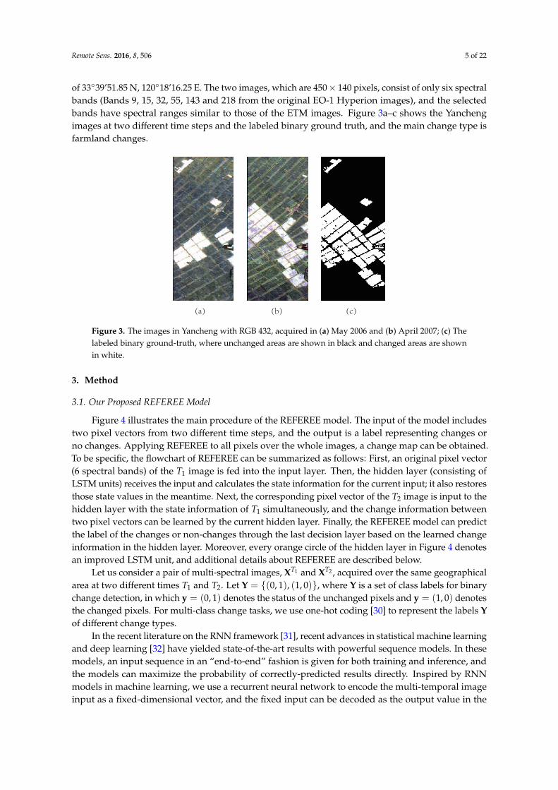
(3) Yancheng images: The third dataset includes two images acquired for the city of Yancheng,China, in May 2006 (t1) and April 2007 (t2), with a WGS-84 projection and approximate coordinates

Remote Sens. 2016, 8, 506 5 of 22

of 33◦39’51.85 N, 120◦18’16.25 E. The two images, which are 450× 140 pixels, consist of only six spectralbands (Bands 9, 15, 32, 55, 143 and 218 from the original EO-1 Hyperion images), and the selectedbands have spectral ranges similar to those of the ETM images. Figure 3a–c shows the Yanchengimages at two different time steps and the labeled binary ground truth, and the main change type isfarmland changes.

(a) (b) (c)

Figure 3. The images in Yancheng with RGB 432, acquired in (a) May 2006 and (b) April 2007; (c) Thelabeled binary ground-truth, where unchanged areas are shown in black and changed areas are shownin white.

3. Method

3.1. Our Proposed REFEREE Model

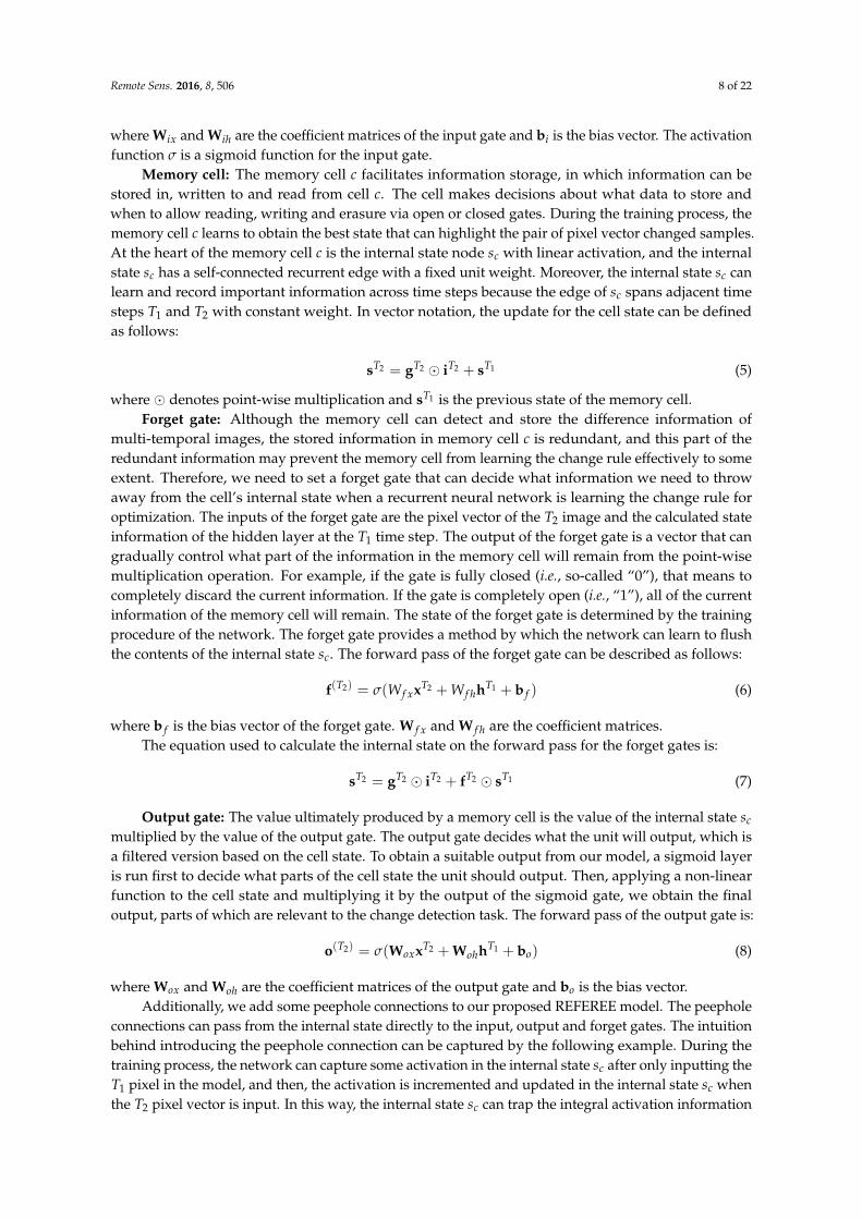
Figure 4 illustrates the main procedure of the REFEREE model. The input of the model includestwo pixel vectors from two different time steps, and the output is a label representing changes orno changes. Applying REFEREE to all pixels over the whole images, a change map can be obtained.To be specific, the flowchart of REFEREE can be summarized as follows: First, an original pixel vector(6 spectral bands) of the T1 image is fed into the input layer. Then, the hidden layer (consisting ofLSTM units) receives the input and calculates the state information for the current input; it also restoresthose state values in the meantime. Next, the corresponding pixel vector of the T2 image is input to thehidden layer with the state information of T1 simultaneously, and the change information betweentwo pixel vectors can be learned by the current hidden layer. Finally, the REFEREE model can predictthe label of the changes or non-changes through the last decision layer based on the learned changeinformation in the hidden layer. Moreover, every orange circle of the hidden layer in Figure 4 denotesan improved LSTM unit, and additional details about REFEREE are described below.

Let us consider a pair of multi-spectral images, XT1 and XT2 , acquired over the same geographicalarea at two different times T1 and T2. Let Y = {(0, 1), (1, 0)}, where Y is a set of class labels for binarychange detection, in which y = (0, 1) denotes the status of the unchanged pixels and y = (1, 0) denotesthe changed pixels. For multi-class change tasks, we use one-hot coding [30] to represent the labels Yof different change types.

In the recent literature on the RNN framework [31], recent advances in statistical machine learningand deep learning [32] have yielded state-of-the-art results with powerful sequence models. In thesemodels, an input sequence in an “end-to-end” fashion is given for both training and inference, andthe models can maximize the probability of correctly-predicted results directly. Inspired by RNNmodels in machine learning, we use a recurrent neural network to encode the multi-temporal imageinput as a fixed-dimensional vector, and the fixed input can be decoded as the output value in the

Remote Sens. 2016, 8, 506 6 of 22

training process. During the training step, the change rule of REFEREE can be learned in context layerswith transferability.

Input Layer

Hidden Layer

Decision Layer

Recurrent connection

Recurrent Neural NetworkImages

T1 Image

T2 Image

Pixel Pair Qualitative Result

Change Map

1st

2nd

Time Sequence

Figure 4. The framework overview of the proposed REFEREE change detection model.

Thus, the probability of obtaining the correct predicted results can be maximized directly formulti-temporal images XT1 and XT2 using the following formulation:

θ∗ = arg maxθ

∑i

p(yi|xT1i , xT2

i ; θ) (1)

where θ is the parameter set of our model, xT1i and xT2

i denote a pair of pixel vectors of the multi-spectralimages XT1 and XT2 and yi is the predicted label.

We input xT1i and xT2

i into the model as time sequence data; thus, it is natural to model p(yi|xT1i , xT2

i )

with a recurrent neural network, where the change rule is expressed by a fixed-length hidden stateor memory ht. The memory is updated with a new pixel vector input using a non-linear function f ,which can be described as:

ht+1 = f (ht, xt) (2)

The important advantage of a recurrent neural network is its ability to sense contextualinformation when mapping the input sequence and output.

3.2. LSTM Hidden Unit and Forward Pass of the REFEREE Model

The choice of f is critical for vanishing and exploding gradient [33] issues, which are a commonchallenge in designing and training a recurrent neural network. The LSTM model [27] is beneficialfor preventing the above problems and performs well when applied to many challenging problemsinvolving sequential time series data. Thus, in this paper, a special LSTM model is improved for therecurrent hidden unit to address change detection for multi-temporal remote sensing data.

According to the characteristics of the change detection task, a detailed architecture of the LSTMunit is designed, as shown in Figure 5. Here, REFEREE learns the reliable difference information ina core memory cell using multi-temporal images, and the core memory cell is jointly modulated bythree gates: input, output and forget gates. These gates determine the amount of dynamic informationentering, leaving and updating the memory cell. In particular, the forget gate can update the internaldifference information of the core memory cell. The output, which exits from the core memory cell,

Remote Sens. 2016, 8, 506 7 of 22

shows a reliable capability in terms of the expression of difference information extraction. Moreover,the core memory cell can recode and highlight the value of the binary changed samples or multi-classchanges in the update process to detect changes with transferability. Additional details about the threegates are given below.

Figure 5. The structure of the LSTM unit in our REFEREEmodel, in which gray arrows indicate directedconnection, where the information will flow along this direction, and a gray dotted arrow indicates apeephole connection. Additional details are available in the text.

The core of the LSTM unit is a memory cell c, which encodes the difference information aboutthe change rule. The behavior of the cell is controlled by three gates: input, output and forget gates.The gates are layers that can either decide to keep the current cell state value if the gate is 1 or to cleanthe memory from the gated layer if the gate is 0. Three gates are generally used to control the input,output and update of the current cell state value in the memory cell. The output of the memory cellcontains the change information. The definition of the three gates, memory cell and final output aredescribed below.

Input node: This unit, which is labeled gt, is a node that responds to activation from the inputlayer at the current time step T2 and from the hidden layer at the previous time step T1. The nodemerges the information at two different times and inputs this information into the cell. This unit canbe formulated as follows:

g(T2) = φ(WgxxT2 + WghhT1 + bg) (3)

where Wgx and Wgh are coefficient matrices and bg is the bias vector of the input node. φ is theactivation function of the input node, the tanh function.

Gates are an important concept in LSTM. A gate is a sigmoidal unit that responds to activationfrom the pixel vector of T2 images, as well as from the hidden layer at the T1 time step. All gates inREFEREE are used to multiply the input to decide whether to pass or cut off the input value. In brief, ifthe value of any gate is “one” (the gate is fully open), then all of the flow is passed through. In contrast,if the value of the gate is “zero” (the gate is fully closed), the flow of the other input is cut off.

Input gate: The input gate is checked to decide whether an input should be read to the memorycell. The value of the input gate multiplies the current time pixel vector and the output of the hiddenlayer at the previous time step T1. The pixel vectors usually contain abundant information; however,only parts of this information are beneficial for distinguishing changes or change types. Therefore,the input gate can automatically select useful information and input it into memory cell c to learn thechange rule. The forward pass of the input gate is:

i(T2) = σ(WixxT2 + WihhT1 + bi) (4)

Remote Sens. 2016, 8, 506 8 of 22

where Wix and Wih are the coefficient matrices of the input gate and bi is the bias vector. The activationfunction σ is a sigmoid function for the input gate.

Memory cell: The memory cell c facilitates information storage, in which information can bestored in, written to and read from cell c. The cell makes decisions about what data to store andwhen to allow reading, writing and erasure via open or closed gates. During the training process, thememory cell c learns to obtain the best state that can highlight the pair of pixel vector changed samples.At the heart of the memory cell c is the internal state node sc with linear activation, and the internalstate sc has a self-connected recurrent edge with a fixed unit weight. Moreover, the internal state sc canlearn and record important information across time steps because the edge of sc spans adjacent timesteps T1 and T2 with constant weight. In vector notation, the update for the cell state can be definedas follows:

sT2 = gT2 � iT2 + sT1 (5)

where � denotes point-wise multiplication and sT1 is the previous state of the memory cell.Forget gate: Although the memory cell can detect and store the difference information of

multi-temporal images, the stored information in memory cell c is redundant, and this part of theredundant information may prevent the memory cell from learning the change rule effectively to someextent. Therefore, we need to set a forget gate that can decide what information we need to throwaway from the cell’s internal state when a recurrent neural network is learning the change rule foroptimization. The inputs of the forget gate are the pixel vector of the T2 image and the calculated stateinformation of the hidden layer at the T1 time step. The output of the forget gate is a vector that cangradually control what part of the information in the memory cell will remain from the point-wisemultiplication operation. For example, if the gate is fully closed (i.e., so-called “0”), that means tocompletely discard the current information. If the gate is completely open (i.e., “1”), all of the currentinformation of the memory cell will remain. The state of the forget gate is determined by the trainingprocedure of the network. The forget gate provides a method by which the network can learn to flushthe contents of the internal state sc. The forward pass of the forget gate can be described as follows:

f(T2) = σ(W f xxT2 + W f hhT1 + b f ) (6)

where b f is the bias vector of the forget gate. W f x and W f h are the coefficient matrices.The equation used to calculate the internal state on the forward pass for the forget gates is:

sT2 = gT2 � iT2 + fT2 � sT1 (7)

Output gate: The value ultimately produced by a memory cell is the value of the internal state sc

multiplied by the value of the output gate. The output gate decides what the unit will output, which isa filtered version based on the cell state. To obtain a suitable output from our model, a sigmoid layeris run first to decide what parts of the cell state the unit should output. Then, applying a non-linearfunction to the cell state and multiplying it by the output of the sigmoid gate, we obtain the finaloutput, parts of which are relevant to the change detection task. The forward pass of the output gate is:

o(T2) = σ(WoxxT2 + WohhT1 + bo) (8)

where Wox and Woh are the coefficient matrices of the output gate and bo is the bias vector.Additionally, we add some peephole connections to our proposed REFEREE model. The peephole

connections can pass from the internal state directly to the input, output and forget gates. The intuitionbehind introducing the peephole connection can be captured by the following example. During thetraining process, the network can capture some activation in the internal state sc after only inputting theT1 pixel in the model, and then, the activation is incremented and updated in the internal state sc whenthe T2 pixel vector is input. In this way, the internal state sc can trap the integral activation information

Remote Sens. 2016, 8, 506 9 of 22

from the T1 pixel vector and the T2 pixel vector. If there are changed pixels, the network will recordsome difference information in the internal state, and the internal state will provide feedback to theaffected output gate. In this way, the internal state sc is the input of ot, and the output gate will offeran optimized value for the final output of this model to detect changed samples more easily, which iswhy the peephole connection is important to the REFEREE model.

The forward pass of an LSTM unit is defined as follows:Input node:

g(T2) = φ(WgxxT2 + WghhT1 + bg) (9)

Input gate:i(T2) = σ(WixxT2 + WihhT1 + WicsT1 + bi) (10)

where Wic is the coefficient matrix of the peephole connection that links the input gate and cell.Forget gate:

f(T2) = σ(W f xxT2 + W f hhT1 + W f csT1 + b f ) (11)

where W f c is the peephole connection matrix of the forget gate and memory cell.Output gate:

o(T2) = σ(WoxxT2 + WohhT1 + WocsT1 + bo) (12)

where Woc is the peephole connection matrix of the output gate and cell c.Cell output:

sT2 = gT2 � iT2 + fT2 � sT1 (13)

LSTM output:hT2 = φ(sT2)� oT2 (14)

To better understand the internal operation modes of a recurrent neural network, we unroll theloop, as shown in Figure 6. Its chain-like nature reveals that the recurrent network is intimately relatedto the sequence, and the natural architecture of a neural network is a promising way of addressingchange detection tasks for multi-temporal images.

Input T1 Input T2

Output T1 Output T2

Input t

Output t

Figure 6. An unrolled recurrent neural network.

3.3. Optimization

Suppose that we have a loss l that we wish to minimize at time step T2 and that the loss l dependson the output of decision layer y and the ground truth label y via a loss function f :

l = f (yT2 , y) (15)

Remote Sens. 2016, 8, 506 10 of 22

where f can be any differentiable loss function, such as the Euclidean loss:

l = f (yT2 , y) = ‖yT2 − y‖2 (16)

Our ultimate goal in this case is to use gradient descent to minimize the loss L over the twoimages XT1 and XT2 :

L =T2

∑t=T1

l(t) (17)

We now work through the algebra to compute the loss gradient dLdw , where w is a scalar parameter

of the model. Because the loss l = f (yT2 , y) only depends on the values of the decision layer y, hiddenlayer h and ground truth label y, we define the chain rule:

dLdw

=T2

∑t=T1

N

∑j=1

M

∑i=1

dLdyj(t)

dyj(t)dhi(t)

dhi(t)dw

(18)

where hi(t) is the scalar corresponding to the i-th hidden output of the memory cell, M is the totalnumber of memory cells, yj(t) is the j-th unit of the decision layer and N is the number of decisionlayer units. Because the network propagates information forward in time, changing yj(t) and hi(t)will not affect the loss prior to time t, which allows us to write:

dLdyj(t)

=T2

∑s=T1

dl(s)dyj(t)

=T2

∑s=t

dl(s)dyj(t)

(19)

For notational convenience, we introduce the variable L(t), which represents the cumulative lossfrom time step t onward:

L(t) =s=T2

∑s=t

l(s) (20)

In this case, L(T1) is the loss for both images XT1 and XT2 , which allows us to rewrite Equation (19) as:

dLdyj(t)

=T2

∑s=t

dl(s)dyj(t)

=dL(t)dyj(t)

(21)

We can now define the gradient calculation dLdw as follows:

dLdw

=T2

∑t=T1

N

∑j=1

M

∑i=1

dL(t)dyj(t)

dyj(t)dhi(t)

dhi(t)dw

(22)

The computation of dhi(t)dw and

dyj(t)dhi(t)

follows directly from the forward propagation equations.

The key question is how to compute dL(t)dyj(t)

. In this paper, we utilize back-propagation using the

time algorithm to resolve these issues. First, we can express the following recursion based on thevariable L(t):

L(t) =

{l(t) + L(t + 1) t < T

l(t) t = T(23)

Hence, given the activation h of an LSTM node at time step t, we have that:

dL(t)dy(t)

=dl(t)dy(t)

+dL(t + 1)

dy(t)(24)

Remote Sens. 2016, 8, 506 11 of 22

The first term dl(t)dy(t) is simply the element-wise derivative of the loss l(t) with respect to the

activations y(t) at time step t. The second term dL(t+1)dy(t) is the recurrent nature of LSTM, which shows

that we need the derivative information of the next node to compute the derivative information ofthe current node. Because dL(t)

dy(t) for both times T1 and T2 is to be computed, we start by computingdL(T2)dy(T2)

= dl(T2)dy(T2)

and work backward through the network.

4. Experimental Setup and Design

This section is structured as follows: (1) describing the competitors (comparison methods);(2) tuning the parameters of the REFEREE model and competitors; and (3) arranging the wholeexperimental design for the study of the sensitivity of REFEREE.

4.1. Competitors

In this paper, the results obtained using the REFEREE method are compared to those from severalother methods: (1) unsupervised Change Vector Analysis (CVA) [8], which is an effective methodfor multi-spectral change detection tasks; (2) PCA [34], which is simple in computation and canbe applied to real-time applications; (3) Iteratively-Reweighted Multivariate Alteration Detection(IRMAD) [15], which is a classical transformation change detection method for multi-spectral data;(4) Supervised Slow Feature Analysis (SSFA) [19], which is one of the latest feature learning methodsfor change detection; (5) Support Vector Machine (SVM) [35], which is effective for remote-sensingimage classification; (6) decision tree [36], which is a tree structure consisting of internal and terminalnodes that process data to ultimately yield a classification; and (7) Convolutional Neural Network(CNN) [37], which is a hierarchical architecture trained on large-scale datasets and that has shownpromising performance in classification and detection. Among these methods, CVA, PCA, IRMAD andSSFA are used in binary experiments, and SVM, decision tree and CNN are compared to REFEREEin multi-class experiments. Additionally, the proposed REFEREE method and other methods areevaluated based on kappa coefficients, the Overall Accuracy (OA) value and the F-score.

4.2. Setup of Parameters

The REFEREE model is trained with the RMSpropalgorithm [38], and the suggested defaultparameters are used for all of the following experiments. In REFEREE, we use a single-layer LSTMof size 512 with sigmoid gate activations and tanh activation for hidden representations, where thesigmoid gate activations and tanh activation are both default settings under the RNN framework. Thedecision layer uses sigmoid activation and then outputs a two-dimensional vector for binary changedetection tasks and three- and four-dimensional vectors for Kunshan and Taizhou multi-class changetasks. All weight matrices in our model and the bias vector are initialized from a uniform distribution,and the values of these weight matrices and the bias vector are initialized in the range [−0.1, 0.1]. Then,all of the weight matrices and bias vectors can be updated during learning processing. In addition, weuse dropout with a probability of 0.5 on the output of each LSTM to avoid overfitting.

Concerning the competitors, the threshold is an important parameter in the CVA, PCA, IRMADand SSFA methods, and k-means clustering [39] is selected for automatic threshold selection. In thebinary experiments, changes and non-changes can be regarded as a two-class classification problem [19].Therefore, the number k in k-means clustering is two. For the SVM method, LibSVM [35] is selected toevaluate the final multi-class changes, where the kernel is the radial basis function, the cost parameter is100 and gamma is 0.01. For the decision tree method in this paper, the maximum tree count parameteris 50, the minimum number of objects per leaf is two and the confidence factor for pruning is 0.1.For the CNN method, the parameters (i.e., the weights in the convolutional and FC layers) are trainedwith classic stochastic gradient descent based on the back-propagation algorithm [40].

Remote Sens. 2016, 8, 506 12 of 22

4.3. Experimental Design

To demonstrate the effectiveness of REFEREE, three experiments are designed in this paper:binary experiments, transfer experiments and multi-class change experiments.

Binary experiments: We select some training samples from multi-temporal images to test thechange detection results derived from the remaining samples. The final results are represented interms of the average accuracy acquired from ten trials, which rely on ten initial randomly-selectedtraining samples from the T1 image and the corresponding initial samples from the T2 image.Wu et al. [19] had labeled some test samples according to a detailed visual analysis of multi-temporalimages and some prior information, and these labeled samples are also used to quantitatively evaluatethe performance of REFEREE and its competitors. For each trial, additional details about the numberof training samples, testing samples and all labeled test samples are summarized in Table 1, whereunits of un denote unchanged samples and units of c denote changed samples.

Table 1. The number of training/testing samples for binary experiments, transfer experiments andmulti-class change experiments on the Taizhou and Kunshan images (the units of un mean unchangedsamples and the units of c mean changed samples). Additional details on the change types andmulti-class definitions can be found in Section 2.

Labeled Samples Training Samples Testing Samples

Taiz

hou

binary 21,116 700experiment (16,890un, 4226c) (500 un,200c) 20,416

200 (150un,50c)transfer 21,116 400 (300un,1000c) 64,183

experiment (16,890un, 4226c) 600 (450un,150c) (Kunshan)

(T-K) 800 (600un,2000c) 63,000(T-Y) 1000 (650un,250c) (Yancheng)

3172 (city change) 200 2922multi-class 564 (soil change) 50 514experiment 490 (water change) 50 440

16,890 (unchanged) 50 11890

Kun

shan

binary 64,183 1000experiment (48,119un, 16,064c) (500un,500 c) 63183

200 (100un,100c)transfer 64,183 400 (200un,200c) 21,116

experiment (48,119un, 16,064c) 600 (300un,300c) (Taizhou)

(K-T) 800 (400un,400c) 63,000(K-Y) 1000 (500un,5000c) (Yancheng)

multi-class 9958 (city change) 500 9458experiment 6506 (farmland change) 500 6006

48,119 (unchanged) 500 43,119

Yanc

heng

binary 63,000 500experiment (44,723un, 18,277c) (250un,250 c) 63,000

200 (100un,100c)transfer 63,000 400 (200un,200c) 21,116

experiment (44,723un, 18,277c) 600 (300un,300c) (Taizhou)

(Y-T) 800 (400un,400c) 64183(Y-K) 1000 (500un,5000c) (Kunshan)

Transfer experiments: The training samples are selected from training multi-temporal images (A),whereas the testing samples are selected from new target multi-temporal images (B, B 6=A) to testwhether the change rule learned from the training multi-temporal images (A) is suitable for newmulti-temporal images (B, B 6=A). This is defined as transferability. In this paper, training images

Remote Sens. 2016, 8, 506 13 of 22

and new target images should have similar multi-spectral distributions (the same number of spectralbands). In the transfer experiments, the REFEREE method is only trained once on the trainingimages (A) and is applicable without further training on arbitrary new target images. Specifically, weselect a set number of training samples from the Taizhou images, and testing samples are selectedfrom all labeled Kunshan samples without any extra information and vice versa. Additionally, tosimulate challenging real-life training and transfer conditions, we provide results for a wide range oftraining data size conditions. In many change detection situations, especially for supervised methods,the training samples may not be sufficiently fine to detect changes over the whole remote sensingdata, and less training data will not result in good features for change detection. Therefore, REFEREEis experimented with over a range of training data sizes. We randomly select 200, 400, 600, 800 and1000 training samples from training images to test the performance on whole labeled test samples ofthe other new images. The final results show the average accuracy acquired from ten trials performedindependently. Additional details about the number of training samples and testing samples can befound in Table 1.

Multi-class change experiments: Regarding change detection as a classification task, we utilizeREFEREE with the input of pixel spectral information from two different time steps, and the outputis the encoded multi-class change information. Additional details about the definition of multi-classchange and change types are described in Section 2. To synthetically evaluate the performance ofREFEREE for multi-class change detection, the numbers of labeled samples, training samples andtesting samples are summarized in Table 1. The final results show the average accuracy acquired fromten trials performed independently.

5. Results and Discussion

This section reports and discusses all of the results of the binary experiments, transfer experimentsand multi-class change experiments.

5.1. Results and Discussion of the Binary Experiments

Figures 7–9 show binary change maps and confidence level maps obtained by REFEREE onthe Taizhou images, the Kunshan images and the Yancheng images, respectively. The binarychange maps in Figures 7a,c, 8a,c and 9a clearly show the main changed regions in the labeled area.Moreover, REFEREE also provides the confidence level of the detected changed samples, as shownin Figures 7b,d, 8b,d and 9b. In the confidence level maps, the brighter the color is, the greater theprobability that the sample belongs to the changed sample. In contrast, a darker color indicates alower probability that the sample is a changed sample. For example, white in the confidence levelmap indicates that the probability that the sample is a changed sample is one (i.e., 100 percentageprobability), whereas black indicates that the probability that the sample is a changed sample iszero. A value between zero and one indicates a different probability or confidence level that thesample is a changed sample. From the confidence level maps of the changed region, it can also befound that changed regions almost all have a highlighted value, whereas unchanged regions arevery dark. The confidence values spread mostly over the two terminal values (zero and one), andthe intermediate values are limited. Therefore, it can be concluded that the REFEREE method candistinguish the changed and unchanged regions directly with the reliable difference learning ability inthe core memory cell.

Table 2 summarizes the kappa coefficients and OA values using all of the methods on thetwo experimental datasets of the labeled samples, and the highest accuracy is obtained by REFEREE.The classical approaches CVA, PCA, IRMAD and SSFA all achieve a good performance, especiallythe SSFA method, which achieves the best performance for single-band analysis [19]. However, fora real-life remote sensing analysis process, we prefer to use all of the spectral information to detectchanges with high accuracy rather than attempt using each band and select the best-performing bandto detect changes. This is because it is very difficult to test and select suitable bands from a very large

Remote Sens. 2016, 8, 506 14 of 22

remote sensing dataset individually. Here, REFEREE uses all available spectral bands and yields thebest performance among all methods.

（a） （b）

0

0.1

0.2

0.3

0.4

0.5

0.6

0.7

0.8

0. 9

1

（c） （d）0

0.1

0.2

0.3

0.4

0.5

0.6

0.7

0.8

0. 9

1

Figure 7. The thematic maps obtained from REFEREE with the Taizhou images: (a) binary changemap of the whole images, where black indicates unchanged regions and white indicates changedregions; (b) confidence level map of the whole Taizhou image, where the color bar is described inthe text; (c) binary change map of the labeled samples, where white indicates changed regions, grayindicates unchanged regions and black indicates unlabeled regions; (d) confidence level map of thelabeled samples.

（c） （d）（a） （b）0

0.1

0.2

0.3

0.4

0.5

0.6

0.7

0.8

0. 9

1

0

0.1

0.2

0.3

0.4

0.5

0.6

0.7

0.8

0. 9

1

Figure 8. The thematic maps obtained using REFEREE for the Kunshan images: (a) binary change mapof the whole images, where black indicates non-changes and white indicates changes; (b) confidencelevel map of the whole Kunshan images, where the color bar is described in the text; (c) binary changemap of labeled samples, where white indicates changed regions, gray indicates unchanged regions andblack indicates unlabeled regions; (d) confidence level map of the labeled samples.

0.1

0.2

0.3

0.4

0.5

0.6

0.7

0.8

0.9

1

（a） （b）

Figure 9. The thematic maps obtained using REFEREE for the Yancheng images: (a) binary change mapof the whole images, where black indicates non-changes and white indicates changes; (b) confidencelevel map of the whole Kunshan images, where the color bar is described in the text.

Remote Sens. 2016, 8, 506 15 of 22

Table 2. The kappa coefficients for the state-of-the-art methods on the two experimental datasets. CVA,Change Vector Analysis; IRMAD, Iteratively-Reweighted Multivariate Alteration Detection; SSFA,Supervised Slow Feature Analysis.

TaiZhou KunShan Yancheng

KAPPA OA KAPPA OA KAPPA OA

CVA 0.3755 0.6982 0.4011 0.7160 0.7907 0.8722PCA 0.5413 0.7419 0.633 0.7741 0.8174 0.9025

IRMAD 0.7942 0.9133 0.87 0.9397 0.6973 0.8352SSFA 0.8229 0.9454 0.9361 0.9763 0.9032 0.9516

REFEREE 0.9477 0.9777 0.9573 0.9837 0.9563 0.9828

5.2. Results and Discussion of the Transfer Experiments

An efficient change rule should have robust transferability. In this experimental part, REFEREE isapplied to the transfer experiments, and the results show that REFEREE has remarkable transferability.From Section 5.1, it can be seen that REFEREE yields a good performance on the Taizhou images (T),Kunshan images (K) and Yancheng images (Y), with a reliable change learning ability in the binaryexperiments. If the learned change rule used by REFEREE is stable and robust, it should yield efficienttransferability for new target images. Therefore, the transfer experimental results are presented anddiscussed in this subsection.

Six transfer experiments, the T-K, T-Y, K-T, K-Y, Y-T and Y-K transfer experiments, are designedwith cross-validation over three images in this section. Here, T denotes Taizhou images, K denotesKunshan images and Y denotes Yancehng images. Specifically, for the K-T transfer experiments, thetraining samples are selected from the Kunshan images, whereas the testing samples are all of thelabeled Taizhou samples. Similarly, in the T-K transfer experiments, the training samples are selectedfrom the Taizhou images, and the testing samples are all of the labeled Kunshan samples. By thatanalogy, the K-Y, T-Y, Y-T and Y-K transfer experiments can be understood clearly.

Additionally, to simulate challenging real-world training conditions, we provide results for a widerange of training dataset size conditions. We report the results over a range of training numbers (N) totest the final transfer results. For example, an N value of 200 (N = 200) indicates that only 200 trainingsamples (100 unchanged samples and 100 changed samples) are selected from the training images(Taizhou or Kunshan) to test all labeled test samples in the new target images (Kunshan or Taizhou).Similarly, an N value of 1000 (N = 1000) indicates that 1000 training samples (500 unchanged samplesand 500 changed samples) are used in the transfer experiments.

Table 3 summarizes the transfer results over five training data sizes in six transfer experiments.Moreover, five indices are used to provide a quantitative analysis of the change detection results:Overall Accuracy (OA), False Positives (FPs), False Negatives (FNs), Overall Error (OE) andKappacoefficients [41]. Generally, the different training data sizes available yield different results. Weprefer a very high performance with a small number of training samples rather than a large numberof samples in deep learning. The proposed method can be used widely. Note that, from Table 3,REFEREE can yield a good performance in all transfer experiments over the five training data sizeranges. For all transfer experiments, the OE value is stable and even shows some slight downwardtrend with increasing number of training samples, which indicates that REFEREE can also offer a goodperformance with small training data sizes in the transfer experiments. Moreover, compared to theFN values of the training data sizes, the FP values are much smaller, which means that REFEREE candetect almost all changed samples directly. In particular, it can be found that the K-T, K-Y and T-Ytransfer experiments yield better results than the T-K, Y-K and Y-T transfer experiments; in particular,the FP values in the K-T, T-Y and K-Y experiments are higher than those in the T-K, Y-T and Y-Kexperiments. The reason for this is related to the complexity of land cover changes in the training steps,which means that the Kunshan images present more complex changes than do the Taizhou imagesand Yancheng images. In addition, REFEREE can learn a more stable change rule from the Kunshan

Remote Sens. 2016, 8, 506 16 of 22

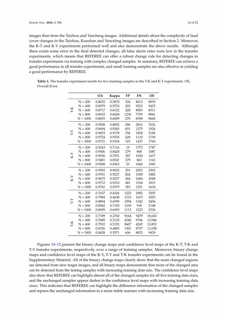
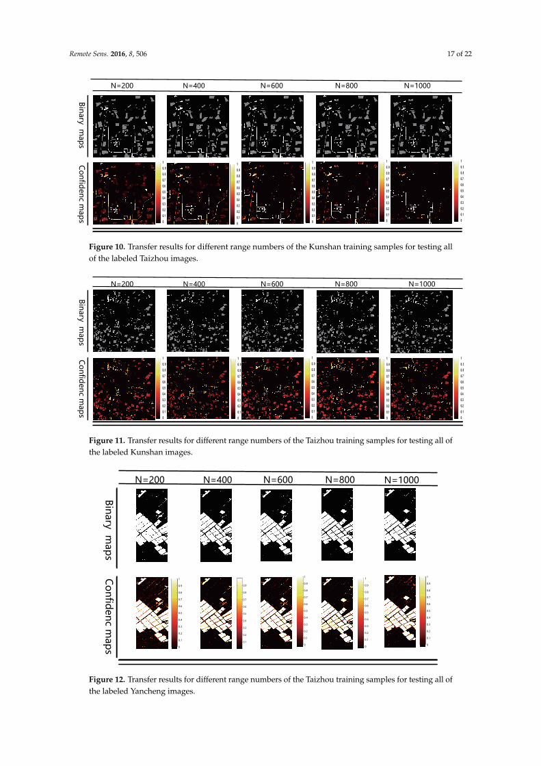
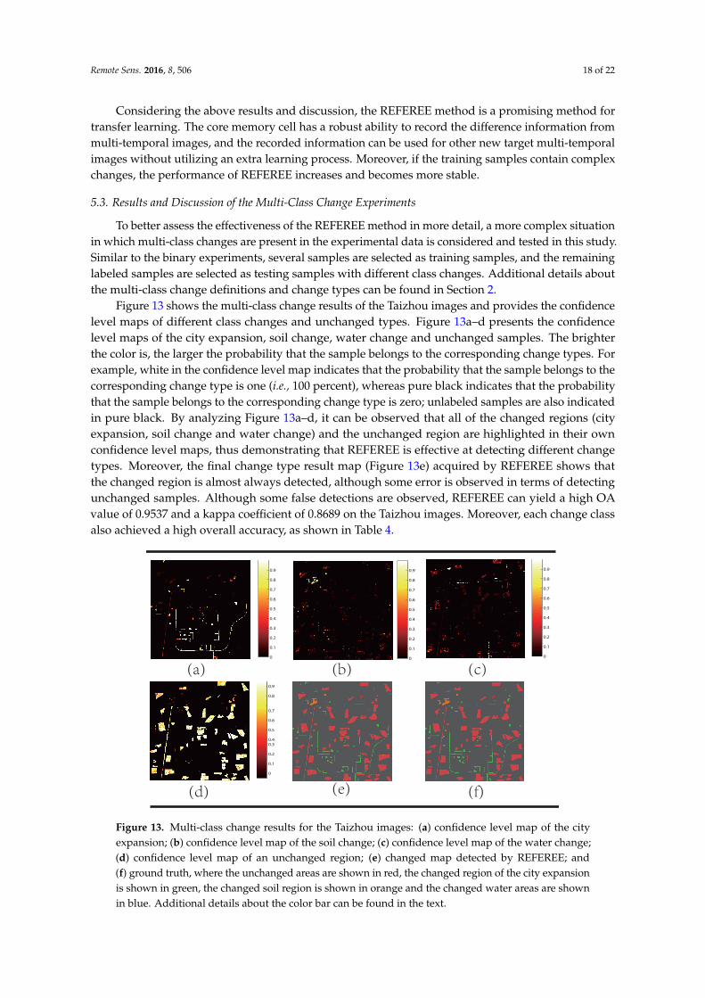
images than from the Taizhou and Yancheng images. Additional details about the complexity of landcover changes in the Taizhou, Kunshan and Yancehng images are described in Section 2. Moreover,the K-T and K-Y experiments performed well and also demonstrate the above results. Althoughthere exists some error in the final detected changes, all false alarm rates were low in the transferexperiments, which means that REFEREE can offer a robust change rule for detecting changes intransfer experiments via training with complex changed samples. In summary, REFEREE can achieve agood performance in all transfer experiments, and small training samples are also effective at yieldinga good performance by REFEREE.

Table 3. The transfer experiment results for five training samples in the T-K and K-T experiments. OE,Overall Error.

OA Kappa FP FN OE

T-K

N = 200 0.8652 0.5870 326 8613 8939N = 400 0.8579 0.5574 202 9223 9425N = 600 0.8717 0.6122 428 8083 8511N = 800 0.8652 0.6028 1236 7705 8941N = 1000 0.8693 0.6009 270 8398 8668

T-Y

N = 200 0.9508 0.8852 286 2816 3102N = 400 0.9694 0.9265 651 1275 1926N = 600 0.9653 0.9178 356 1828 2184N = 800 0.9724 0.9335 629 1110 1739N = 1000 0.9721 0.9334 323 1437 1760

K-T

N = 200 0.9243 0.7116 15 1772 1787N = 400 0.9506 0.8428 279 808 1087N = 600 0.9536 0.7931 387 1030 1417N = 800 0.9481 0.8341 279 863 1141N = 1000 0.9508 0.8363 23 1060 1083

K-Y

N = 200 0.9592 0.9032 251 2052 2303N = 400 0.9701 0.9227 824 1058 1882N = 600 0.9675 0.9227 364 1684 2048N = 800 0.9712 0.9310 481 1334 1815N = 1000 0.9741 0.9379 383 1251 1634

Y-T

N = 200 0.7637 0.4326 1223 2982 3205N = 400 0.7984 0.4638 1210 1815 3025N = 600 0.8894 0.6559 1094 1342 2436N = 800 0.8942 0.7100 1230 918 2148N = 1000 0.8939 0.6993 1113 1223 2336

Y-K

N = 200 0.7189 0.2760 9164 9479 18,643N = 400 0.7689 0.3125 4240 9706 13,946N = 600 0.7932 0.5152 9607 4245 13,852N = 800 0.8336 0.4883 1301 9737 11,038N = 1000 0.8428 0.5571 606 8823 9429

Figures 10–12 present the binary change maps and confidence level maps of the K-T, T-K andT-Y transfer experiments, respectively, over a range of training samples. Moreover, binary changemaps and confidence level maps of the K-Y, T-Y and T-K transfer experiments can be found in theSupplementary Material. All of the binary change maps clearly show that the main changed regionsare detected from new target images, and all binary maps demonstrate that more of the changed areacan be detected from the testing samples with increasing training data size. The confidence level mapsalso show that REFEREE can highlight almost all of the changed samples for all five training data sizes,and the unchanged samples appear darker in the confidence level maps with increasing training datasizes. This indicates that REFEREE can highlight the difference information of the changed samplesand repress the unchanged information in a more stable manner with increasing training data size.

Remote Sens. 2016, 8, 506 17 of 22

0

0.1

0.2

0.3

0.4

0.5

0.6

0.7

0.8

0. 9

1

0

0.1

0.2

0.3

0.4

0.5

0.6

0.7

0.8

0. 9

1

0

0.1

0.2

0.3

0.4

0.5

0.6

0.7

0.8

0. 9

1

0

0.1

0.2

0.3

0.4

0.5

0.6

0.7

0.8

0. 9

1

0

0.1

0.2

0.3

0.4

0.5

0.6

0.7

0.8

0. 9

1

Figure 10. Transfer results for different range numbers of the Kunshan training samples for testing allof the labeled Taizhou images.

0

0.1

0.2

0.3

0.4

0.5

0.6

0.7

0.8

0. 9

1

0

0.1

0.2

0.3

0.4

0.5

0.6

0.7

0.8

0. 9

1

0

0.1

0.2

0.3

0.4

0.5

0.6

0.7

0.8

0. 9

1

0

0.1

0.2

0.3

0.4

0.5

0.6

0.7

0.8

0. 9

1

0

0.1

0.2

0.3

0.4

0.5

0.6

0.7

0.8

0. 9

1

Figure 11. Transfer results for different range numbers of the Taizhou training samples for testing all ofthe labeled Kunshan images.

0

0.1

0.2

0.3

0.4

0.5

0.6

0.7

0.8

0.9

1

0.1

0.2

0.3

0.4

0.5

0.6

0.7

0.8

0.9

0

0.1

0.2

0.3

0.4

0.5

0.6

0.7

0.8

0.9

1

0

0.1

0.2

0.3

0.4

0.5

0.6

0.7

0.8

0.9

1

0

0.1

0.2

0.3

0.4

0.5

0.6

0.7

0.8

0.9

1

Figure 12. Transfer results for different range numbers of the Taizhou training samples for testing all ofthe labeled Yancheng images.

Remote Sens. 2016, 8, 506 18 of 22

Considering the above results and discussion, the REFEREE method is a promising method fortransfer learning. The core memory cell has a robust ability to record the difference information frommulti-temporal images, and the recorded information can be used for other new target multi-temporalimages without utilizing an extra learning process. Moreover, if the training samples contain complexchanges, the performance of REFEREE increases and becomes more stable.

5.3. Results and Discussion of the Multi-Class Change Experiments

To better assess the effectiveness of the REFEREE method in more detail, a more complex situationin which multi-class changes are present in the experimental data is considered and tested in this study.Similar to the binary experiments, several samples are selected as training samples, and the remaininglabeled samples are selected as testing samples with different class changes. Additional details aboutthe multi-class change definitions and change types can be found in Section 2.

Figure 13 shows the multi-class change results of the Taizhou images and provides the confidencelevel maps of different class changes and unchanged types. Figure 13a–d presents the confidencelevel maps of the city expansion, soil change, water change and unchanged samples. The brighterthe color is, the larger the probability that the sample belongs to the corresponding change types. Forexample, white in the confidence level map indicates that the probability that the sample belongs to thecorresponding change type is one (i.e., 100 percent), whereas pure black indicates that the probabilitythat the sample belongs to the corresponding change type is zero; unlabeled samples are also indicatedin pure black. By analyzing Figure 13a–d, it can be observed that all of the changed regions (cityexpansion, soil change and water change) and the unchanged region are highlighted in their ownconfidence level maps, thus demonstrating that REFEREE is effective at detecting different changetypes. Moreover, the final change type result map (Figure 13e) acquired by REFEREE shows thatthe changed region is almost always detected, although some error is observed in terms of detectingunchanged samples. Although some false detections are observed, REFEREE can yield a high OAvalue of 0.9537 and a kappa coefficient of 0.8689 on the Taizhou images. Moreover, each change classalso achieved a high overall accuracy, as shown in Table 4.

0

0.1

0.2

0.3

0.4

0.5

0.6

0.7

0.8

0.9

0

0.1

0.2

0.3

0.4

0.5

0.6

0.7

0.8

0.9

0

0.1

0.2

0.3

0.4

0.5

0.6

0.7

0.8

0.9

0

0.1

0.2

0.3

0.4

0.5

0.6

0.7

0.8

0.9

(a) (b) (c)

(d) (e) (f)

Figure 13. Multi-class change results for the Taizhou images: (a) confidence level map of the cityexpansion; (b) confidence level map of the soil change; (c) confidence level map of the water change;(d) confidence level map of an unchanged region; (e) changed map detected by REFEREE; and(f) ground truth, where the unchanged areas are shown in red, the changed region of the city expansionis shown in green, the changed soil region is shown in orange and the changed water areas are shownin blue. Additional details about the color bar can be found in the text.

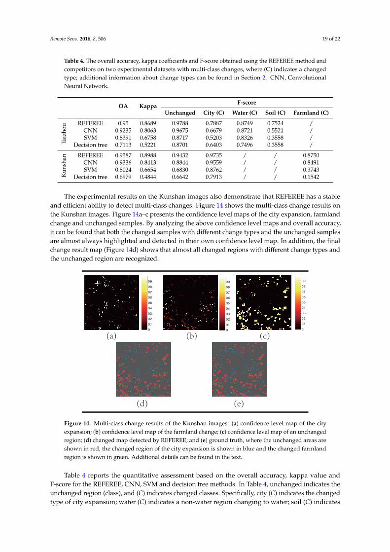
Remote Sens. 2016, 8, 506 19 of 22

Table 4. The overall accuracy, kappa coefficients and F-score obtained using the REFEREE method andcompetitors on two experimental datasets with multi-class changes, where (C) indicates a changedtype; additional information about change types can be found in Section 2. CNN, ConvolutionalNeural Network.

OA Kappa F-score

Unchanged City (C) Water (C) Soil (C) Farmland (C)

Taiz

hou REFEREE 0.95 0.8689 0.9788 0.7887 0.8749 0.7524 /

CNN 0.9235 0.8063 0.9675 0.6679 0.8721 0.5521 /SVM 0.8391 0.6758 0.8717 0.5203 0.8326 0.3558 /

Decision tree 0.7113 0.5221 0.8701 0.6403 0.7496 0.3558 /

Kun

shan REFEREE 0.9587 0.8988 0.9432 0.9735 / / 0.8750

CNN 0.9336 0.8413 0.8844 0.9559 / / 0.8491SVM 0.8024 0.6654 0.6830 0.8762 / / 0.3743

Decision tree 0.6979 0.4844 0.6642 0.7913 / / 0.1542

The experimental results on the Kunshan images also demonstrate that REFEREE has a stableand efficient ability to detect multi-class changes. Figure 14 shows the multi-class change results onthe Kunshan images. Figure 14a–c presents the confidence level maps of the city expansion, farmlandchange and unchanged samples. By analyzing the above confidence level maps and overall accuracy,it can be found that both the changed samples with different change types and the unchanged samplesare almost always highlighted and detected in their own confidence level map. In addition, the finalchange result map (Figure 14d) shows that almost all changed regions with different change types andthe unchanged region are recognized.

0

0.1

0.2

0.3

0.4

0.5

0.6

0.7

0.8

0.9

(a) (b) (c)

(d) (e)

0

0.1

0.2

0.3

0.4

0.5

0.6

0.7

0.8

0.9

0

0.1

0.2

0.3

0.4

0.5

0.6

0.7

0.8

0.9

Figure 14. Multi-class change results of the Kunshan images: (a) confidence level map of the cityexpansion; (b) confidence level map of the farmland change; (c) confidence level map of an unchangedregion; (d) changed map detected by REFEREE; and (e) ground truth, where the unchanged areas areshown in red, the changed region of the city expansion is shown in blue and the changed farmlandregion is shown in green. Additional details can be found in the text.

Table 4 reports the quantitative assessment based on the overall accuracy, kappa value andF-score for the REFEREE, CNN, SVM and decision tree methods. In Table 4, unchanged indicates theunchanged region (class), and (C) indicates changed classes. Specifically, city (C) indicates the changedtype of city expansion; water (C) indicates a non-water region changing to water; soil (C) indicates

Remote Sens. 2016, 8, 506 20 of 22

cultivated field or grassland (or any non-bare soil class) changing to bare soil; and farmland (C)indicates farmland changes. Additional details on the changed types can be found in Section 2. TheSVM and decision tree-based change detection methods performed well in the multi-class changedetection experiments in terms of the OA, kappa and F-score values. However, the CNN-based changedetection method and REFEREE both achieved higher OA, kappa and F-score values. The REFEREEmethod produced the best quantitative assessment in terms of all three indices, which means thatour learned model is an effective way of learning change information based on multi-class changes.In particular, concerning the F-score, for soil (C) and farmland (C), REFEREE achieved a 40% higherF-score than did the SVM and decision tree methods. In addition, CNN also represents a promisingway to learn features and perform classification using artificial neural networks, and our model canperform slightly better than the CNN method in terms of all quantitative assessment indices.

Regarding change detection as a classification task, we utilize REFEREE with pixels from twodifferent time steps as input and the encoded change information as output. As demonstrated bythe above experiments, the REFEREE method achieves a good performance in not only the binaryexperiments, but also the multi-class change experiments.

6. Conclusions

In this paper, a new change detection algorithm named REFEREE that can detect not only binarychanges with stable transferability, but also multi-class changes has been proposed. By introducing andimproving the basic RNN framework with the LSTM model, the proposed REFEREE algorithm canprovide a stable change rule for detecting changes from multi-temporal remote sensing data. Comparedto other state-of-the-art algorithms, the superiority of REFEREE mainly depends on learning a stableand transferable change rule by recording the difference information or multi-class changes in a corememory cell. In addition, as demonstrated by the experimental results in this paper, the superiority ofREFEREE can be summarized through three main contributions as follows: (1) REFEREE can learn astable change rule, and the core memory can record the reliable difference information; (2) comparedto other state-of-the-art algorithms, REFEREE can detect not only binary changes, but also multi-classchanges for multi-temporal images; (3) the REFEREE method also has good transferability for detectingchanges in new target images without any extra learning process. The new target images should havemulti-spectral distributions similar (the same number of spectral bands) to those of the training imagesin this paper.

As demonstrated in this paper, REFEREE is robust and stable when detecting both binary andmulti-class changed samples. However, the method still suffers from various issues. For example,a small number of unchanged samples is mistaken as changed samples; this issue should be resolvedin future work to render REFEREE more effective. We will attempt to improve the REFEREE methodto be able to detect a new changed type when the relevant training samples do not exist.

Acknowledgments: This work was jointly supported by the National Basic Research Program of China(Grant No. 2015CB953703), the National Natural Science Foundation of China (Nos. 41371328, 91537210 and51190092) and the Beijing Higher Education Young Elite Teacher Project (YETP0132). The computation in thiswork is supported by the Tsinghua National Laboratory for Information Science and Technology.

The authors would like to acknowledge the editor and reviewers for their instructive comments, whichhelped to improve this paper. The authors would also like to thank Chen Wu for providing experimental imagery.

Author Contributions: All authors contributed to the design of the experiment and to its undertaking. All authorsrevised and approved the final manuscript.

Conflicts of Interest: The authors declare no conflict of interest.

References

1. Hermosilla, T.; Wulder, M.A.; White, J.C.; Coops, N.C.; Hobart, G.W. Regional detection, characterization,and attribution of annual forest change from 1984 to 2012 using landsat-derived time series metrics.Remote Sens. Environ. 2015, 170, 121–132.

Remote Sens. 2016, 8, 506 21 of 22

2. Singh, A. Digital change detection techniques using remotely-sensed data. Int. J. Remote Sens. 1989, 10,989–1003.

3. Yuan, Y.; Meng, Y.; Lin, L.; Sahli, H; Yue, A.; Chen, J.b.; Zhao, Z.M.; Kong, Y.L.; He, D.X. ContinuousChange Detection and Classification Using Hidden Markov Model: A Case Study for Monitoring UrbanEncroachment onto Farmland in Beijing. Remote Sens. 2015, 7, 15318–15339.

4. Koltunov, A.; Ustin, S.L. Early fire detection using non-linear mul-titemporal prediction of thermal imagery.Remote Sens. Environ. 2007, 110, 18–28.

5. Wen, D.; Huang, X.; Zhang, L.; enediktsson, J.A. A novel automatic changedetection method for urbanhigh-resolution remotely sensed imagery based on multiindex scene representation. IEEE Trans. Geosci.Remote Sens. 2016, 54, 609–625.

6. Shapiro, A.C.; Trettin, C.C.; Küchly, H.; Alavinapanah, S.; Bandeira, S. The Mangroves of the Zambezi Delta:Increase in Extent Observed via Satellite from 1994 to 2013. Remote Sens. 2015, 7, 16504–16518.

7. Robson, B.A.; Holbling, D.; Nuth, C.; Strozzi, T.; Dahl, S.O. Decadal Scale Changes in Glacier Area in theHohe Tauern National Park (Austria) Determined by Object-Based Image Analysis. Remote Sens. 2016, 8,doi:10.3390/rs8010067.

8. Bovolo, F.; Bruzzone, L. A theoretical framework for unsupervised change detection based on change vectoranalysis in the polar domain. IEEE Trnas. Geosci. Remote Sens. 2007, 45, 218–236.

9. Sinha, P.; Kumar, L.; Reid, N. Rank-Based Methods for Selection of Landscape Metrics for Land CoverPattern Change Detection. Remote Sens. 2016, 8, 107, doi:10.3390/rs8020107.

10. Basnet, B.; Vodacek, A. Tracking Land Use/Land Cover Dynamics in Cloud Prone Areas Using ModerateResolution Satellite Data: A Case Study in Central Africa. Remote Sens. 2015, 7, 6683–6709.

11. Demir, B.; Bovolo, F.; Bruzzone, L. Updating land-cover maps by classification of image time series: A novelchange-detection-driven transfer learning approach. IEEE Trans. Geosci. Remote Sens. 2013, 51, 300–312.

12. Ganchev, T.D.; Jahn, O.; Marques, M.I.; Figueired, J.M.; Schuchmann, K.L. Automated acoustic detection ofvanellus chilensis lampronotus. Remote Sens. Environ. 2015, 42, 6098–6111.

13. Morsier, F.; Tuia, D.; Borgeaud, M.; Gass, V.; Thiran , J.P. Semi-supervised novelty detection using svm entiresolution path. IEEE Trans. Geosci. Remote Sens. 2013, 51, 1939–1950.

14. Parmentier, B. Characterization of Land Transitions Patterns from Multivariate Time Series Using SeasonalTrend Analysis and Principal Component Analysis. Remote Sens. 2014, 6, 12639–12665.

15. Nielsen, A.A. The regularized iteratively reweighted mad method for change detection in multi- andhyperspectral data. IEEE Trans. Image Process. 2007, 16, 463–478.

16. Wu, C.; Du, B.; Zhang, L. A subspace-based change detection method for hyperspectral images. IEEE J. Sel.Top. Appl. Earth Obs. Remote Sens. 2013, 6, 815–830.

17. Bouaraba, A.; Aissa, A.B.; Borghys, D.; Acheroy, M.; Closson, D. Insar phase filtering via joint subspaceprojection method: Application in change detection. IEEE Geosci. Remote Sens. Lett. 2014, 11, 1817–1820.

18. Erturk, A.; Iordache, M.D.; Plaza, A. Sparse unmixing-based change detection for multitemporalhyperspectral images. IEEE J. Sel. Top. Appl. Earth Obs. Remote Sens. 2015, 9, 708–719.

19. Wu, C.; Du, B.; Zhang, L. Slow feature analysis for change detection in multispectral imagery. IEEE Trans.Geosci. Remote Sens. 2014, 52, 2858–2874.

20. Meola, J.; Eismann, M.T.; Moses, R.L.; Ash, J.N. Application of model-based change detection to airborneVNIR/SWIR hyperspectral imagery. IEEE Trans. Geosci. Remote Sens. 2012, 50, 3693–3706.

21. Huang, X.; Friedl, M.A. Distance metric-based forest cover change detection using modis time series. Int. J.Appl. Earth Obs. Geoinf. 2014, 29, 78–92.

22. Byun, Y.; Han, Y.; Chae, T. Image Fusion-Based Change Detection for Flood Extent Extraction UsingBi-Temporal Very High-Resolution Satellite Images. Remote Sens. 2015, 7, 10347–10363.

23. Liu, S.; Bruzzone, L. Hierarchical unsupervised change detection in multitemporal hyperspectral images.IEEE Trans. Geosci. Remote Sens. 2015, 53, 244–260.

24. Shah-Hosseini, R.; Homayouni, S.; Safari, A. A Hybrid Kernel-Based Change Detection Method for RemotelySensed Data in a Similarity Space. Remote Sens. 2015, 7, 12829–12858.

25. Ding, K.; Huo, C. Sparse hierarchical clustering for vhr image change detection. IEEE Geosci. Remote Sens. Lett.2015, 12, 577–581.

Remote Sens. 2016, 8, 506 22 of 22

26. Fu, X.; Li, S.; Fairbank, M.; Wunsch, D.C.; Alonso, E. Training Recurrent Neural Networks with theLevenberg—Marquardt Algorithm for Optimal Control of a Grid-Connected Converter. IEEE Trans. NeuralNetw. Learn. Syst. 2014, 26, 1900–1912.

27. Ordónez, F.J.; Roggen, D. Deep Convolutional and LSTM Recurrent Neural Networks for MultimodalWearable Activity Recognition. Sensors 2016, 16, 115.

28. Ubeyli, E. Recurrent neural networks with composite features for detection of electrocardiographic changesin partial epileptic patients. Comput. Biol. Med. 2008, 38, 401–410.

29. Pacella, M.; Semeraro, Q. Using recurrent neural networks to detect changes in autocorrelated processes forquality monitoring. Comput. Ind. Eng. 2007, 52, 502–520.

30. Chren, W. One-hot residue coding for high-speed non-uniform pseudo-random test pattern generation.In Proceedings of the 1995 IEEE International Symposium on Circuits and Systems (ISCAS ’95),Seattle, WA, USA, 30 April–3 May 1995; Volume 1, pp. 401–404.

31. Brillante, C.; Mannarino, A. Improvement of aeroelastic vehicles performance through recurrent neuralnetwork controllers. Nonlinear Dyn. 2016, 84, 1479–1495.

32. Yuan, Y.; Mou, L.; Lu, X. Scene Recognition by Manifold Regularized Deep Learning Architecture.IEEE Trans. Neural Netw. Learn. Syst. 2015, 26, 2222–2233.

33. Pascanu, R.; Mikolov T.; Bengio Y. On the difficulty of training recurrent neural networks. In Proceedings ofthe IEEE International Conference on Machine Learning, Atlanta, GA, USA, 16–21 June 2013; pp. 1310–1318.

34. Deng, J.; Wang, K.; Deng, Y.; Qi, G. Pca-based land-use change detection and analysis using multitemporaland multisensor satellite data. Int. J. Remote Sens. 2008, 29, 4823–4838.

35. Chang, C.; Lin, C. LIBSVM: A Library for Support Vector Machines. ACM Trans. Intell. Syst. Technol. 2011, 2,1–27.

36. Pal, M.; Mather, P. An assessment of the effectiveness of decision tree methods for land cover classification.Remote Sens. Environ. 2003, 86, 554–565.

37. Hu, F.; Xia, G.-S.; Hu, J.; Zhang, L. Transferring Deep Convolutional Neural Networks for the SceneClassification of High-Resolution Remote Sensing Imagery. Remote Sens. 2015, 7, 14680–14707.

38. Dauphin, Y.N.; Vries, H.; Chung, J.; Bengio, Y. Rmsprop and equilibrated adaptive learning rates fornon-convex optimization. 2015, arXiv:1502.04390.

39. Celik, T. Unsupervised change detection in satellite images using principal component analysis and k-meansclustering.IEEE Geosci. Remote Sens. Lett. 2009, 6, 772–776.

40. Rumelhart, D.E.; Hintont, G.E.; Williams, R.J. Learning representations by back-propagating errors. Nature1986, 323, 533–536.

41. Congalton, R.G. A review of assessing the accuracy of classifications of remotely sensed data.Remote Sens. Environ. 1991, 37, 35–46.

c© 2016 by the authors; licensee MDPI, Basel, Switzerland. This article is an open accessarticle distributed under the terms and conditions of the Creative Commons Attribution(CC-BY) license (http://creativecommons.org/licenses/by/4.0/).