learning a predictable and generative vector ... · pdf filelearning a predictable and...

Learning a Predictable and GenerativeVector Representation for Objects

Rohit Girdhar1 David F. Fouhey1 Mikel Rodriguez2 Abhinav Gupta1

1Robotics Institute, Carnegie Mellon University 2MITRE Corporation{rgirdhar,dfouhey,abhinavg}@cs.cmu.edu, [email protected]

Abstract. What is a good vector representation of an object? We be-lieve that it should be generative in 3D, in the sense that it can producenew 3D objects; as well as be predictable from 2D, in the sense that it canbe perceived from 2D images. We propose a novel architecture, called theTL-embedding network, to learn an embedding space with these proper-ties. The network consists of two components: (a) an autoencoder thatensures the representation is generative; and (b) a convolutional net-work that ensures the representation is predictable. This enables tack-ling a number of tasks including voxel prediction from 2D images and3D model retrieval. Extensive experimental analysis demonstrates theusefulness and versatility of this embedding.

1 Introduction

What is a good vector representation for objects? On the one hand, there hasbeen a great deal of work on discriminative models such as ConvNets [18, 32]mapping 2D pixels to semantic labels. This approach, while useful for distinguish-ing between classes given an image, has two major shortcomings: the learnedrepresentations do not necessarily incorporate the 3D properties of the objectsand none of the approaches have shown strong generative capabilities. On theother hand, there is an alternate line of work focusing on learning to generateobjects using 3D CAD models and deconvolutional networks [5, 19]. In contrastto the purely discriminative paradigm, these approaches explicitly address the3D nature of objects and have shown success in generative tasks; however, theyoffer no guarantees that their representations can be inferred from images andaccordingly have not been shown to be useful for natural image tasks. In thispaper, we propose to unify these two threads of research together and proposea new vector representation (embedding) of objects.

We believe that an object representation must satisfy two criteria. Firstly, itmust be generative in 3D: we should be able to reconstruct objects in 3D fromit. Secondly, it must be predictable from 2D: we should be able to easily inferthis representation from images. These criteria are often at odds with each other:modeling occluded voxels in 3D is useful for generating objects but very difficultto predict from an image. Thus, optimizing for only one criterion, as in most pastwork, tends not to obtain the other. In contrast, we propose a novel architecture,

2 R. Girdhar, D. F. Fouhey, M. Rodriguez and A. Gupta

(a) (b)

Fig. 1: (a) We learn an embedding space that has generative capabilities to con-struct 3D structures, while being predictable from RGB images. (b) Our finalmodel’s 3D reconstruction results on natural and synthetic test images.

the TL-embedding network, that directly optimizes for both criteria. We achievethis by building an architecture that has two major components, joined via a 64-dimensional (64D) vector embedding space: (1) An autoencoder network whichmaps a 3D voxel grid to the 64D embedding space, and decodes it back to a voxelgrid; and (2) A discriminatively trained ConvNet that maps a 2D image to the64D embedding space. By themselves, these represent generative and predictablecriteria; by joining them, we can learn a representation that optimizes both.

At training time, we take the 3D voxel map of a CAD model as well as its2D rendered image and jointly optimize the components. The auto-encoder aimsto reconstruct the voxel grid and the ConvNet aims to predict the intermediateembedding. The TL-network can be thought of as a 3D auto-encoder that triesto ensure that the 3D representation can be predicted from a 2D rendered image.At test time, we can use the autoencoder and the ConvNet to obtain a represen-tation for 3D voxels and images respectively in the common latent space. Thisenables us to tackle a variety of tasks at the intersection of 2D and 3D.

We demonstrate the nature of our learned embedding in a series of experi-ments on both CAD model data and natural images gathered in-the-wild. Ourexperiments demonstrate that: (1) our representation is indeed generative in 3D,permitting reconstruction of novel CAD models; (2) our representation is pre-dictable from 2D, allowing us to predict the full 3D voxels of an object froman image (an extremely difficult task), as well as do fast CAD model retrievalfrom a natural image; and (3) that the learned space has a number of goodproperties, such as being smooth, carrying class-discriminative information, andallowing vector arithmetic. In the process, we show the importance of our designdecisions, and the value of joining the generative and predictive approaches.

2 Related Work

Our work aims to produce a representation that is generative in 3D and pre-dictable from 2D and thus touches on two long-standing and important questionsin computer vision: how do we represent 3D objects in a vector space and howdo we recognize this representation in images?

Learning a Predictable and Generative Vector Representation for Objects 3

Learning an embedding, or vector representation of visual objects is a wellstudied problem in computer vision. In the seminal work of Olshausen andField [26], the objective was to obtain a representation that was sparse andcould reconstruct the pixels. Since then, there has been a lot of work in thisreconstructive vein. For a long time, researchers focused on techniques such asstacked RBMs or autoencoders [12, 36] or DBMs [30], and more recently, this hastaken the form of generative adversarial models [9]. This line of work, however,has focused on building a 2D generative model of the pixels themselves. In thiscase, if the representation captures any 3D properties, it is modeled implicitly.In contrast, we focus on explicitly modeling the 3D shape of the world. Thus,our work is most similar to a number of recent exceptions to the 2D end-to-endapproach. Dosovitskiy et al. [5] used 3D CAD models to learn a parameterizedgenerative model for objects and Kulkarni et al. [19] introduced a technique toguide the latent representation of a generative model to explicitly model certain3D properties. While they use 3D data like our work, they use it to build agenerative model for 2D images. Our work is complementary: their work cangenerate the pixels for a chair and ours can generate the voxels (and thus, helpan agent or robot to interact with it).

There has been comparatively less work in the 3D generative space. Pastworks have used part-based models [2, 16] and deep networks [39, 20, 24] for rep-resenting 3D models. In contrast to 2D generative models, these approachesacknowledges the 3D structure of the world. However, unlike our work, it doesnot address the mapping from images to this 3D structure. We believe this is acrucial distinction: while the world is 3D, the images we receive are intrinsically2D and we must build our representations with this in mind.

The task of inferring 3D properties from images goes back to the very begin-ning of vision. Learning-based techniques started gaining traction in the mid-2000s [13, 31] by framing it as a supervised problem of mapping images of scenesto 2.5D maps. Among a large body of works trying to infer 3D representationsfrom images, our approach is most related to a group of works using render-ings of 3D CAD models to predict properties such as object viewpoint [35] orclass [34], among others [33, 10, 27]. Typically, these approaches focus on global3D properties such as pose in the case of objects, and 2.5D maps in the case ofscenes. Our work predicts a much more challenging representation, a voxel map(i.e., including the occluded parts). Related works in 3D prediction include [17,38, 3]. Our approach differs from these as it is class agnostic, voxel based andlearns a joint embedding that enables various applications beyond 3D prediction.

Our final output is related to CAD model retrieval in the sense that oneoutput of our approach is a 3D model. Many approaches achieve this via align-ment [23, 1, 14] or joint, but non-generative embeddings [21]. In contrast to theseworks, we take the extreme approach of generating the 3D voxel map from theimage. While we obtain coarser results than using an existing model, this ex-plict generative mapping gives the potential to generalize to previously unseenobjects.


64 F

ull

y C

onnec

ted

Rendered Chairs

20x20x20 Voxel Input

20x20x20 Voxel output

Sigmoid Cross-Entropy Loss

Euclidean Loss

4096 FC 4096 FC

64 FC

256

384

384

256

96

20x20x20 Voxel output

4096 FC 4096 FC

64FC

256

384

384

256

96

Input Image

Train (T-Network)

Test (L-Network)

96

256

384

256 6

96

256

384

256 6

96

256

384

256

Fig. 2: Our proposed TL-embedding network. (a) T-network: At training time,the network takes two inputs: 2D RGB images which are fed into ConvNet atthe bottom and 3D voxel maps which are fed into the autoencoder on the left.The output is a 3D voxel map. We apply two losses jointly: a reconstructionloss for the voxel outputs, and a regression loss for the 64-D embedding in themiddle. (b) L-network: During testing, we remove the encoder part and onlyuse the image as input. The ConvNet predicts the embedding representation andthe decoder predicts the voxel.

3 Our Approach

To reiterate, our goal is to learn a vector representation that is: (a) generative:we should be able to generate voxels in 3D from this representation; and (b)predictable: we should be able to take a 2D image of an object and predictthis representation. Both properties are vital for image understanding tasks.

We propose a novel TL-embedding network (Fig. 2) to optimize both thesecriteria. The T and L refer to the architecture in the training and testing phase.The top part of the T network is an autoencoder with convolution and deconvolu-tion layers. The encoder maps the 3D voxel map to a low-dimensional subspace.The decoder maps a datapoint in the low-dimensional subspace to a 3D voxelmap. The autoencoder forces the embedding to be generative, and we can sampledatapoints in this embedding to reconstruct new objects. To optimize the pre-dictable criterion, we use a ConvNet architecture similar to AlexNet [18], addinga loss function that ensures the embedding space is predictable from pixels.

Training this TL-embedding network requires 2D RGB images and their cor-responding 3D voxel maps. Since this data is hard to obtain, we use CAD modeldatasets to obtain voxel maps and render these CAD models with different ran-dom backgrounds to generate corresponding image data. We now describe ournetwork architecture and the details of our training and testing procedure.


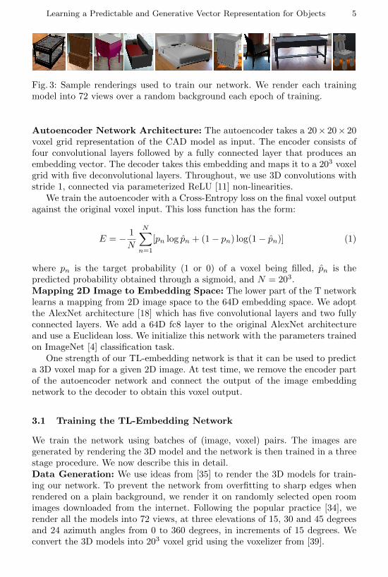
Fig. 3: Sample renderings used to train our network. We render each trainingmodel into 72 views over a random background each epoch of training.

Autoencoder Network Architecture: The autoencoder takes a 20× 20× 20voxel grid representation of the CAD model as input. The encoder consists offour convolutional layers followed by a fully connected layer that produces anembedding vector. The decoder takes this embedding and maps it to a 203 voxelgrid with five deconvolutional layers. Throughout, we use 3D convolutions withstride 1, connected via parameterized ReLU [11] non-linearities.

We train the autoencoder with a Cross-Entropy loss on the final voxel outputagainst the original voxel input. This loss function has the form:

E = − 1

N

N∑n=1

[pn log pn + (1− pn) log(1− pn)] (1)

where pn is the target probability (1 or 0) of a voxel being filled, pn is thepredicted probability obtained through a sigmoid, and N = 203.Mapping 2D Image to Embedding Space: The lower part of the T networklearns a mapping from 2D image space to the 64D embedding space. We adoptthe AlexNet architecture [18] which has five convolutional layers and two fullyconnected layers. We add a 64D fc8 layer to the original AlexNet architectureand use a Euclidean loss. We initialize this network with the parameters trainedon ImageNet [4] classification task.

One strength of our TL-embedding network is that it can be used to predicta 3D voxel map for a given 2D image. At test time, we remove the encoder partof the autoencoder network and connect the output of the image embeddingnetwork to the decoder to obtain this voxel output.

3.1 Training the TL-Embedding Network

We train the network using batches of (image, voxel) pairs. The images aregenerated by rendering the 3D model and the network is then trained in a threestage procedure. We now describe this in detail.Data Generation: We use ideas from [35] to render the 3D models for train-ing our network. To prevent the network from overfitting to sharp edges whenrendered on a plain background, we render it on randomly selected open roomimages downloaded from the internet. Following the popular practice [34], werender all the models into 72 views, at three elevations of 15, 30 and 45 degreesand 24 azimuth angles from 0 to 360 degrees, in increments of 15 degrees. Weconvert the 3D models into 203 voxel grid using the voxelizer from [39].


Table 1: Reconstruction performance using AP on test data.

Chair Table Sofa Cabinet Bed Overall

Proposed (before Joint) 96.4 97.1 99.1 99.3 94.1 97.6Proposed (after Joint) 96.4 97.0 99.2 99.3 93.8 97.6

PCA 94.8 96.7 98.6 99.0 91.5 96.8

Three-stage Training: Training a TL-embedding network from scratch andjointly is a challenging problem. Therefore, we take a three stage procedure. (1)In the first stage, we train the autoencoder part of the network independently.This network is initialized at random, and trained end-to-end with the sigmoidcross-entropy loss. We train this for about 200 epochs. (2) In the second stagewe train the ConvNet to regress to the 64D representation. Specifically, theencoder generates the embedding for the voxel and the image network is trainedto regress the embedding. The image network is initialized using ImageNet pre-trained weights. We keep the lower convolutional layers fixed. (3) In the finalstage, we finetune the network jointly with both the losses. In this stage, weobserve that the prediction loss reduces significantly while reconstruction lossreduces marginally. We also observe that most of the parameter update happensin the autoencoder network, indicating that the autoencoder updates its latentrepresentation to make it easily predictable from images, while maintaining orimproving the reconstruction performance given this new latent representation.Implementation Details: We implement this network using the Caffe [15]toolbox. In the first stage, we initialize all layers of autoencoder network fromscratch using N (0, 0.01) and train with a uniform learning rate of 10−6. Next,we train the image network by initializing fc8 from scratch and remaining layersfrom ImageNet. We finetune all layers after and including conv4 with a uni-form learning rate of 10−8. A lower learning rate is required because the initialprediction loss values are in the range of 500K. The encoder network from theautoencoder is used in testing-phase with its previously learned weights to gen-erate the labels for image network. Finally, we jointly train using both losses,initializing the network using weights learned earlier, and finetuning all layers ofautoencoder and all layers after and including conv4 for image network with alearning rate of 10−10. Since our network now has two losses, we balance theirvalues by scaling the autoencoder loss to have approximately same initial value,as otherwise the network tends to optimize for the prediction loss without regardto the reconstruction loss.

4 Experiments

We now experimentally evaluate the method. Our overarching goal is to answerthe following questions: (1) is the representation we learn generative in 3D? (2)can the representation be predicted from images in 2D? In addition to directlyanswering these questions, we verify that the model has learned a sensible latent


Tes

t M

odel

P

CA

-64

Auto

enco

der

Fig. 4: Reconstructions of random test models using PCA and the autoencoder.Predicted voxels are colored and sized by confidence of prediction, from largeand red to small and blue in decreasing order of confidence. PCA is much lessconfident about the extent as well as fine details as compared to our autoencoder.

representation by ensuring that the latent representation satisfies a number ofproperties, such as being smooth, discriminative and allowing arithmetic.

We note that our approach has a capability that, to the best of our knowledge,is previous unexplored: it can simultaneously reconstruct in 3D and predict from2D. Thus, there are no standard baselines or datasets for this task. Instead,we adopt standard datasets for each of the many tasks that our model canperform. Where appropriate, we compare the method with existing methods.These baselines, however, are specialized solutions to only one of the many taskswe can solve and often use additional supervisory information. As the communitystarts tackling increasingly difficult 3D problems like direct voxel prediction, webelieve that our work can be a strong baseline to benchmark progress.

We proceed as follows. We introduce the datasets and evaluation criterionthat we use in Sec. 4.1. We first verify that our learned representation models thespace of voxels well in a number of ways: that it is reconstructive, smooth, andcan be used to distinguish different classes of objects (Sec. 4.2). This evaluatesthe representation independently of its ability to predict voxels from images.We then verify that our approach can predict the voxels from 2D and showthat it outperforms alternate options (Sec. 4.3). Subsequently, we show that ourrepresentation can be used to do CAD retrieval from natural images (Sec. 4.4)and is capable of performing 3D shape arithmetic (Sec. 4.5).

4.1 Datasets and Evaluation

We use two datasets for evaluation. The first is a CAD model dataset used totrain the TL-embedding and to explore the learned embedding. The second isan in-the-wild dataset used to verify that the approach works on natural images.CAD Dataset: We use CAD models from the ShapeNet[39] database. Thisdatabase contains over 220K models organized into 3K WordNet synsets. Wetake a set of common indoor objects: chair (6778 models), table (8509 models),sofa (3173 models), cabinet (1572 models), and bed (254 models). We split thesemodels randomly into 16228 train and 4058 test objects. All our models are


A B---interpolation---

(a)

A B Generated Latent NN

(b)

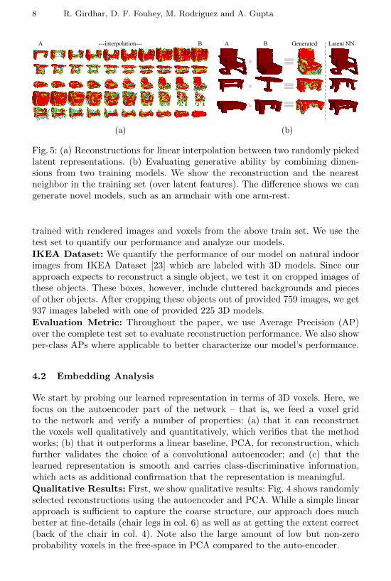
Fig. 5: (a) Reconstructions for linear interpolation between two randomly pickedlatent representations. (b) Evaluating generative ability by combining dimen-sions from two training models. We show the reconstruction and the nearestneighbor in the training set (over latent features). The difference shows we cangenerate novel models, such as an armchair with one arm-rest.

trained with rendered images and voxels from the above train set. We use thetest set to quantify our performance and analyze our models.

IKEA Dataset: We quantify the performance of our model on natural indoorimages from IKEA Dataset [23] which are labeled with 3D models. Since ourapproach expects to reconstruct a single object, we test it on cropped images ofthese objects. These boxes, however, include cluttered backgrounds and piecesof other objects. After cropping these objects out of provided 759 images, we get937 images labeled with one of provided 225 3D models.

Evaluation Metric: Throughout the paper, we use Average Precision (AP)over the complete test set to evaluate reconstruction performance. We also showper-class APs where applicable to better characterize our model’s performance.

4.2 Embedding Analysis

We start by probing our learned representation in terms of 3D voxels. Here, wefocus on the autoencoder part of the network – that is, we feed a voxel gridto the network and verify a number of properties: (a) that it can reconstructthe voxels well qualitatively and quantitatively, which verifies that the methodworks; (b) that it outperforms a linear baseline, PCA, for reconstruction, whichfurther validates the choice of a convolutional autoencoder; and (c) that thelearned representation is smooth and carries class-discriminative information,which acts as additional confirmation that the representation is meaningful.

Qualitative Results: First, we show qualitative results: Fig. 4 shows randomlyselected reconstructions using the autoencoder and PCA. While a simple linearapproach is sufficient to capture the coarse structure, our approach does muchbetter at fine-details (chair legs in col. 6) as well as at getting the extent correct(back of the chair in col. 4). Note also the large amount of low but non-zeroprobability voxels in the free-space in PCA compared to the auto-encoder.


We next show that the learned space is smooth, by computing reconstructionsfor linear interpolation between latent representations of randomly picked testmodels. As Fig. 5(a) shows, the 3D models smoothly transition in structure andmost intermediate models are also physically plausible. We also show resultsexploring the learned space and verifying whether the dimensions are meaningful.One way to do this is to generate new points in the space and reconstruct them.We generate these points by taking the first 32 dimensions from one model andthe rest from another. As seen by the difference between the reconstruction andthe nearest model in Fig. 5(b), this can generate previously unseen models thatcombine aspects of each model.

We further attempt to understand the embedding space by clamping allthe dimensions of a latent vector but one and scaling the selected dimension byadding a fixed value to it. We show its effect on two dimensions and three modelsin Fig. 6. Such scaling of these dimensions produces consistent effects acrossmodels, suggesting that some learned dimensions are semantically meaningful.

Quantitative Reconstruction Accuracy: We now evaluate the reconstruc-tion performance quantitatively on the CAD test data and report results inTable 1. Our goal here is to verify that the auto-encoder is worthwhile: we thuscompare to PCA using the same number of dimensions. Our method obtainsextremely high performance, 97.6% AP and consistently outperforms PCA, re-ducing the average error rate by 25% relative. It can be seen in Table 1 thatsome categories are easier than others: sofas and cabinets are naturally moreeasy than beds (including bunk-beds) and chairs. Our method consistently ob-tains larger gains on challenging objects, indicating the merits of a non-linearrepresentation. We also evaluate the performance of the autoencoder after thejoint training. Even after being optimized to be more predictable from imagespace, we can see that it still preserves the overall reconstruction performance.

CAD Classification: If our representation models 3D well, it should permit usto distinguish different types of objects. We empirically verify this by using ourapproach without modifications as a representation to classify 3D shapes. Notethat while adding a classification loss and finetuning might further improve re-sults, it would defeat the purpose of this experiment, which is to see whether themodel learns a good 3D representation on its own. We evaluate our represen-tation’s performance for a classification task on the Princeton ModelNet40 [28]dataset with standard train-test split from [39]. We train the network on all 40classes (again: no class information is provided) and then use the autoencoderrepresentation as a feature for 40-way classification. Since our representationis low-dimensional (64D), we expand the feature to include pairwise featuresand train a linear SVM. Our approach obtains an accuracy of 74.4%. This iswithin 2.6% of [39], a recent approach on voxels that uses class information atrepresentation-learning time, and finetunes the representation discriminativelyfor the classification experiment. Using a 64D PCA representation trained onModelNet40 trainset with the same feature augmentation and linear SVM ob-tains 68.4%. This shows that our representation is class-discriminative despitenot being trained or designed so, and outperforms the PCA.


D=22 D=9

Fig. 6: We evaluate if the dimensions are meaningful by scaling each dimensionseparately and analyzing the effect on the reconstruction. Some dimensions havea consistent effect on reconstruction across objects. Higher values in dimension22 lead to thicker legs, and higher values in 9 lead to disappearance of legs.

Table 2: Average Precision for Voxel Prediction on the CAD test set. The Pro-posed TL-Network outperforms the baselines on each object.

Chair Table Sofa Cabinet Bed Average

Proposed (with Joint) 66.9 59.7 79.3 79.3 41.9 65.4Proposed (without Joint) 66.6 57.5 79.3 76.5 33.8 62.7

Direct-conv4 40.9 23.7 58.1 44.3 23.1 38.0Direct-fc8 21.8 15.5 35.6 32.7 18.6 24.8

4.3 Voxel Prediction

We now turn to the task of predicting a 3D voxel grid from an image. Weobtain strong performance on this task and outperform a number of baselines,demonstrating the importance of each part of our approach.Baselines: To the best of our knowledge, there are no methods that directly pre-dict voxels from an image; we therefore compare to a direct prediction method aswell an ablation study, where we do not perform joint training. Specifically: (a)Direct: finetuning the ImageNet pre-trained AlexNet to predict the 203 voxel griddirectly. This corresponds to removing the auto-encoder. We tried two strate-gies for freezing the layers: Direct-conv4 refers to freezing all layers before conv4and Direct-fc8 refers to freezing all layers except fc8. (b) Without Joint: train-ing the T-L network without the final joint fine-tuning (i.e., following only thefirst two training stages). The direct baselines test whether the auto-encoder’slow-dimensional representation is necessary and the without-joint tests whetherlearning the model to be jointly generative and predictable is important.Qualitative Results: We first show qualitative results on natural images in Fig.7. Note that our method automatically predicts occluded regions of the object,unlike most work on single image 3D (e.g., [31, 13, 7, 6, 8, 37]) that predict a 2.5Dshell. For instance, our method predicts all four legs of furniture even if fewer are


Fig. 7: Reconstruction results on the IKEA dataset. Our model generalizes wellto real images, even to bookshelves which our model is not trained on.

Table 3: Average Precision for Voxel Prediction on the IKEA dataset.

Bed Bookcase Chair Desk Sofa Table Overall

Proposed 56.3 30.2 32.9 25.8 71.7 23.3 38.3Direct-conv4 38.2 26.6 31.4 26.6 69.3 19.1 31.1

Direct-fc8 29.5 17.3 20.4 19.7 38.8 16.0 19.8

visible. Our model generalizes well to natural images even though it was trainedon CAD models. Note that for instance, the round and rectangular tables arepredicted as being round and rectangular, and office chairs on a single post andfour-legged chairs can be distinguished. One difficulty with this data is thatobjects are truncated or occluded and some windows contain multiple objects;our model does well on this data, nonetheless.Quantitative Results: We now evaluate the approach quantitatively on bothdatasets. We report results on the CAD dataset in Table 2. Our approach out-performs all the baselines. Directly predicting the voxels does substantially worsebecause predicting all the voxels is a very difficult task compared to our embed-ding space. Not doing joint training produces worse results because the embed-ding is not forced to be predictable.

The IKEA dataset is more challenging because it is captured in-the-wild, butour approach still produces quantitatively strong performance. While the CADDataset models are represented in canonical form, the IKEA models are providedin no consistent orientation. We thus attempt to align each prediction with the


Kar’15 Ours Kar’15 Ours Kar’15 Ours

Fig. 8: Predictions on PASCAL 3D+ images using [17] and our method. Ourmethod is better at capturing fine stylistic details, like the straight legs and thehollow back in the first case, a single central leg in the second, and no visiblelegs in the last.

Fig. 9: Top CAD model retrievals from natural images from the IKEA dataset.

ground-truth model by taking the best rigid alignment over permutations, flipsand translational alignments (up to 10%) of the prediction. As Table 3 shows, ourapproach outperforms the direct prediction by a large margin (38% compared to31%). If we do not correct for translational alignments, we still outperform thebaseline (33% vs 28%). Directly predicting voxels again performs worse comparedto predicting the latent space and reconstructing, validating the idea of using alower-dimensional representation of objects.Comparison with Kar et al. [17]: We also compare our method with [17]on PASCAL 3D+ v1.0 [40] dataset for categories that overlap with our trainingcategories (chair and sofa). As Fig. 8 shows, our output is more varied andcaptures stylistic details better. For quantitative comparison, we voxelize theiroutput and ground truth, and compute the overlap P-R curve with alignment.Since [17] produces a binary non-probabilistic prediction and thus yields onlyone operating point, we compare via maximum F-1 score instead of AP. Afteraligning, we outperform their method 0.492 to 0.463.

4.4 CAD Retrieval

We now show results for retrieving CAD models from natural images. Our systemcan naturally tackle this task: we map each model in the CAD corpus as well as


Chair Bed Sofa Bookcase Table/DeskIn

stance

0 50 100 150 200 2500

20

40

60

80

100

120

140

0 50 100 150 200 2500

5

10

15

20

25

0 50 100 150 200 2500

10

20

30

40

50

60

70

80

0 50 100 150 200 2500

20

40

60

80

100

120

140

0 50 100 150 200 2500

10

20

30

40

50

60

70

80

Category

0 50 100 150 200 2500

50

100

150

200

250

0 50 100 150 200 2500

5

10

15

20

25

0 50 100 150 2000

20

40

60

80

100

120

140

160

0 50 100 150 200 2500

50

100

150

200

250

300

0 50 100 150 200 2500

50

100

150

200

250

Fig. 10: Histograms over position in retrieval list obtained by our proposed ap-proach (Y axis: #images, X axis: position). First row of histograms is over theposition of instance match, and second is over position of category match.

Table 4: Mean recall @10 of ground truth model in retrievals for our methodand baseline described in Sec. 4.4

Sofa Chair Bookcase Bed Table Overall

Proposed 32.3 41.0 26.8 38.5 8.0 29.3Fc7-NN 14.6 33.9 23.5 7.7 17.4 19.4

the image to their latent representations, and perform a nearest neighbor searchin this embedding space.

We use cosine distance in the latent space for retrieval. This approach is com-plementary to approaches like [23, 22]: these approaches assume the existence ofan exact-match 3D model and fits the 3D model into the image. Our approach,on the other hand, does not assume exact match and thus generalizes to retriev-ing the most similar object to the depicted object (i.e., what is the next-mostsimilar object in the corpus). We show qualitative results in Fig. 9.

We now quantitatively evaluate our approach. For each test window, we rankall 225 CAD models in the corpus by cosine distance. We can then determinetwo quantities: (a) Instance match: at what rank does the exact-match CADmodel appear? (b) Category match: at what rank does the first model of the samecategory appear? As a baseline, we render all the 225 models at 30 deg. elevationand 8 uniformly sampled azimuths from 0 to 360 deg. onto a white background,after scaling and translating each model to a unit square at the origin. We thenuse ImageNet trained AlexNet’s fc7 features over the query image and renderingsto perform nearest neighbor search (cosine distance). The first position at whicha rendering of a model appears in the retrievals is taken as the position for thatmodel. Note that this is a strong baseline with access to lot more informationsince it sees images, which are much higher resolution than our 203 voxel grids.Moreover, it is significantly slower than our method, as it represents each 3Dmodel using 8 vectors of 4096D each, while our approach uses only a single 64D


Fig. 11: Results of shape arithmetic. In the first case, adding a cabinet-like-tableto a table and removing small 2-leg table results in a table with built-in cabinet.In the second case, adding and removing a similar looking chair with straightand curved edges respectively leads to a table with curved edges.

vector. As shown in Table 4, which reports the mean recall@10 of instance match,we outperform this baseline on all categories except tables/desks because most ofthe table models are very similar, and fine differentiation between specific modelsis very hard for a coarse 203 voxel representation. We report histograms of theseranks in Fig. 10 per object category. For many categories, the top response isthe correct category, and the exact-match model is typically ranked highly. Poorperformance tends to result from images containing multiple objects (e.g., a tablepicture with chairs in it), causing the network to predict the representation forthe “wrong” object out of the ambiguous input. We also compare our modelwith [21] in the supplement available on the project webpage.

4.5 Shape Arithmetic

We have shown that the latent space is reconstructive and smooth, that itis predictable, and that it carries class information. We now show some at-tempts at probing the learned representation. Previous work in vector embed-ding spaces [29, 25] exhibit the phenomena of being able to perform arithmeticon these vector representations. For example, [25] showed that vector(King) -vector(Man) + vector(Woman) results in vector whose nearest neighbor wasthe vector for Queen. We perform a similar experiment by randomly selectingtriplets of 3D models and performing this a + b − c operation on their latentrepresentations. We then use the resulting feature to generate the voxel repre-sentation and also find the nearest neighbor in the dataset over cosine distanceon this latent representation. We show some interesting triplets in Fig. 11.Acknowledgments: This work was partially supported by Siebel Scholarship to RG,

NDSEG Fellowship to DF and Bosch Young Faculty Fellowship to AG. This material

is based on research partially sponsored by ONR MURI N000141010934, ONR MURI

N000141612007, NSF1320083 and a gift from Google. The authors would like to thank

Yahoo! and Nvidia for the compute cluster and GPU donations respectively. The au-

thors would also like to thank Martial Hebert and Xiaolong Wang for many helpful

discussions.


References

1. Aubry, M., Maturana, D., Efros, A., Russell, B., Sivic, J.: Seeing 3D chairs: exem-plar part-based 2D-3D alignment using a large dataset of cad models. In: CVPR(2014)

2. Chaudhuri, S., Kalogerakis, E., Guibas, L., Koltun, V.: Probabilistic reasoning forassembly-based 3D modeling. SIGGRAPH (2011)

3. Choy, C.B., Xu, D., Gwak, J., Chen, K., Savarese, S.: 3d-r2n2: A unified approachfor single and multi-view 3d object reconstruction. CoRR abs/1604.00449 (2016)

4. Deng, J., Dong, W., Socher, R., Li, L.J., Li, K., Fei-Fei, L.: Imagenet: A large-scalehierarchical image database. In: CVPR. pp. 248–255 (2009)

5. Dosovitskiy, A., Springenberg, J., Brox, T.: Learning to generate chairs with con-volutional neural networks. In: CVPR (2015)

6. Eigen, D., Fergus, R.: Predicting depth, surface normals and semantic labels witha common multi-scale convolutional architecture. In: ICCV (2015)

7. Eigen, D., Puhrsch, C., Fergus, R.: Depth map prediction from a single image usinga multi-scale deep network. In: NIPS (2014)

8. Fouhey, D.F., Gupta, A., Hebert, M.: Data-driven 3D primitives for single imageunderstanding. In: ICCV (2013)

9. Goodfellow, I., Pouget-Abadie, J., Mirza, M., Xu, B., Warde-Farley, D., Ozair, S.,Courville, A., Bengio, Y.: Generative adversarial nets. In: NIPS (2014)

10. Gupta, S., Arbelaez, P.A., Girshick, R.B., Malik, J.: Inferring 3D object pose inRGB-D images. CoRR (2015)

11. He, K., Zhang, X., Ren, S., Sun, J.: Delving deep into rectifiers: Surpassing human-level performance on imagenet classification. CoRR abs/1502.01852 (2015)

12. Hinton, G.E., Salakhutdinov, R.R.: Reducing the dimensionality of data with neu-ral networks. Science (2006)

13. Hoiem, D., Efros, A.A., Hebert, M.: Recovering surface layout from an image. In:IJCV (2007)

14. Huang, Q., Wang, H., Koltun, V.: Single-view reconstruction via joint analysis ofimage and shape collections. SIGGRAPH 34(4) (2015)

15. Jia, Y., Shelhamer, E., Donahue, J., Karayev, S., Long, J., Girshick, R., Guadar-rama, S., Darrell, T.: Caffe: Convolutional architecture for fast feature embedding.arXiv preprint arXiv:1408.5093 (2014)

16. Kalogerakis, E., Chaudhuri, S., Koller, D., Koltun, V.: A Probabilistic Model ofComponent-Based Shape Synthesis. SIGGRAPH (2012)

17. Kar, A., Tulsiani, S., Carreira, J., Malik, J.: Category-specific object reconstructionfrom a single image. In: CVPR (2015)

18. Krizhevsky, A., Sutskever, I., Hinton, G.E.: Imagenet classification with deep con-volutional neural networks. In: NIPS. pp. 1097–1105 (2012)

19. Kulkarni, T.D., Whitney, W., Kohli, P., Tenenbaum, J.B.: Deep convolutional in-verse graphics network. In: NIPS (2015)

20. Li, Y., Pirk, S., Su, H., Qi, C.R., J., G.L.: FPNN: Field probing neural networksfor 3d data. CoRR abs/1605.06240 (2016)

21. Li, Y., Su, H., Qi, C.R., Fish, N., Cohen-Or, D., Guibas, L.J.: Joint embeddingsof shapes and images via cnn image purification. ACM TOG (2015)

22. Lim, J.J., Khosla, A., Torralba, A.: FPM: fine pose parts-based model with 3DCAD models. In: ECCV (2014)

23. Lim, J.J., Pirsiavash, H., Torralba, A.: Parsing IKEA objects: Fine pose estimation.In: ICCV (2013)


24. Maturana, D., Scherer, S.: VoxNet: A 3D Convolutional Neural Network for Real-Time Object Recognition. In: IROS (2015)

25. Mikolov, T., Sutskever, I., Chen, K., Corrado, G., Dean, J.: Distributed represen-tations of words and phrases and their compositionality. In: NIPS (2013)

26. Olshausen, B., Field, D.: Emergence of simple-cell receptive field properties bylearning a sparse code for natural images. Nature (1996)

27. Peng, X., Sun, B., Ali, K., Saenko, K.: Exploring invariances in deep convolutionalneural networks using synthetic images. CoRR (2014)

28. Princeton ModelNet: http://modelnet.cs.princeton.edu/29. Radford, A., Metz, L., Chintala, S.: Unsupervised representation learning with

deep convolutional generative adversarial networks. CoRR abs/1511.06434 (2015)30. Salakhutdinov, R., Hinton, G.: Deep Boltzmann machines. In: AISTATS. vol. 5

(2009)31. Saxena, A., Sun, M., Ng, A.Y.: Make3D: Learning 3D scene structure from a single

still image. TPAMI 30(5), 824–840 (2008)32. Simonyan, K., Zisserman, A.: Very deep convolutional networks for large-scale

image recognition. CoRR abs/1409.1556 (2014)33. Stark, M., Goesele, M., Schiele, B.: Back to the future: Learning shape models

from 3D CAD data. In: BMVC (2010)34. Su, H., Maji, S., Kalogerakis, E., Learned-Miller, E.G.: Multi-view convolutional

neural networks for 3d shape recognition. In: ICCV (2015)35. Su, H., Qi, C.R., Li, Y., Guibas, L.J.: Render for CNN: Viewpoint estimation in

images using CNNs trained with rendered 3D model views. In: ICCV (2015)36. Vincent, P., Larochelle, H., Lajoie, I., Bengio, Y., Manzagol, P.A.: Stacked denois-

ing autoencoders: Learning useful representations in a deep network with a localdenoising criterion. J. Mach. Learn. Res. (2010)

37. Wang, X., Fouhey, D.F., Gupta, A.: Designing deep networks for surface normalestimation. In: CVPR (2015)

38. Wu, J., Xue, T., Lim, J.J., Tian, Y., Tenenbaum, J.B., Torralba, A., Freeman,W.T.: Single image 3d interpreter network. In: ECCV (2016)

39. Wu, Z., Song, S., Khosla, A., Yu, F., Zhang, L., Tang, X., Xiao, J.: 3D shapenets:A deep representation for volumetric shapes. In: CVPR (2015)

40. Xiang, Y., Mottaghi, R., Savarese, S.: Beyond pascal: A benchmark for 3d objectdetection in the wild. In: WACV (2014)

learning a predictable and generative vector ... · pdf filelearning a predictable and...

Documents