learning a model of ship movements - uvalearning a model of ship movements university of amsterdam,...
TRANSCRIPT
1
Learning a Model of Ship Movements
University of Amsterdam, Faculty of Science
Science Park 904 Postbus 94216
1090 GE Amsterdam The Netherlands
Thesis for Bachelor of Science - Artificial Intelligence
Author:
Roderik Lagerweij
Supervisors:
Gerben de Vries
Maarten van Someren
December 24, 2009
Keywords Machine Learning, Data Mining, Classification, Time Series Data, Sliding Windows, Discretization,
Attribute Selection, C4.5, Sequential Association-Rule Mining, Automatic Identification System
Abstract In very large seaports, where many ships are entering and leaving the port, collision avoidance is of
utmost importance. A system used to quickly identify ships and to provide additional information is
the Automatic Identification System (AIS). Data Mining methods may be employed to mine AIS
trajectory data for patterns to create a model capable of predicting future events, which can be used
as an extra aid for situational awareness. Two classification methods are proposed and described to
create such model. The final port of a ship entering a large sea port is chosen as future event to
predict. Both presented classification methods significantly outperform the baseline method.

2
1. Introduction In very large sea ports, where many ships are entering and leaving the port, collision avoidance is of
utmost importance. Currently used methods to prevent collisions include visual observation, audio
exchanges and radar. However, the lack of positive identification of other ships and the time delay it
takes to calculate other ships courses prevents a ship from always taking the necessary course
correction to prevent a collision or near collision.
Another system used to quickly identify ships and to provide additional information such as course
and speed is the Automatic Identification System (AIS), a system typically used in marine traffic
monitoring systems. The International Maritime Organization requires every international voyaging
ship that exceeds 300 tons gross tonnage to be equipped with an AIS transponder. As not all ships
are equipped with this transponder, AIS is primarily used as an extra aid for situational awareness
rather than as a fully automatic collision prevention system.
Using data mining methods to mine trajectory data consisting of logged AIS transmissions for
patterns may provide such extra aid for situational awareness. In this research project, two methods
are proposed and described to create a model of ship behavior based on this trajectory data. With
these models, future events can be predicted and anomalous behavior can be detected. To evaluate
the correctness of these predictions, the final dock of a ship entering a very large sea port is chosen
as future event to classify.
The central research question in this paper is:
What is a good method to predict future locations of ships?
To be able to answer this question, we need to know what kind of dataset can be used for these
predictions and what method yields good performance. Here, better performance equals higher
classification accuracies. Furthermore, we should evaluate how predictions less distant or more
distant into the future affect performance.
In the next section, some related work concerning this project is discussed. In section 3, a
characterization of the used dataset is given. In section 4, utilized preprocessing techniques are
described. The two proposed classification methods are described in section 5, along with a basic
comparison between the two and their evaluation and implementation. Up next are the experiments
and their results in section 6. Finally, in section 7 inferred conclusions are presented and possible
future work is discussed in section 8.
3
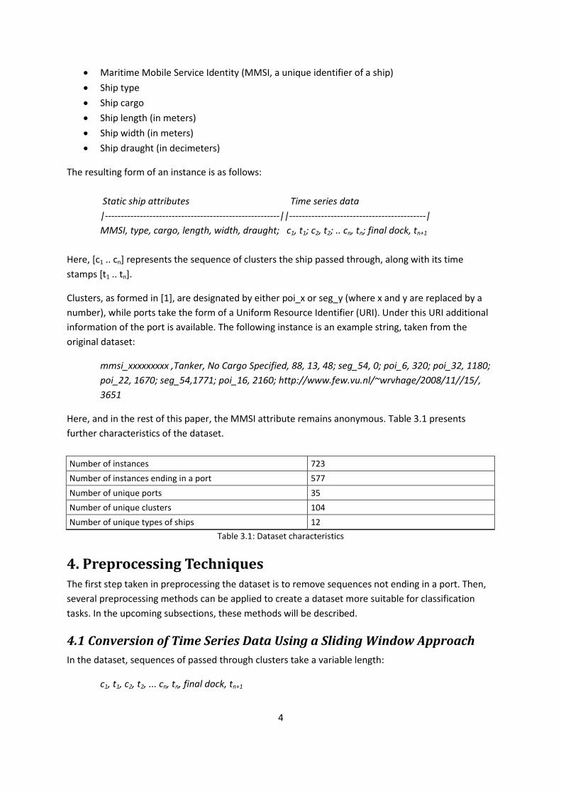
2. Related Work The trajectory data available from the AIS transmissions are spatial time series, describing the
movements of ships entering a very large sea port. Because this type of data is highly regular (e.g.
objects do not jump around) it seems intuitive to compress this data. In [1], de Vries and van
Someren present such an unsupervised method to construct a simple model of ship trajectory data
using compression (Douglas-Puecker, [2]) and clustering (Affinity Propagation) techniques. Figure 2.1
shows an indication of the result, where the green lines represent the clusters and the red lines the
data these clusters are based on.
Figure 2.1: The effect of applying clustering methods as proposed in [1]
3. Dataset The supplied dataset used in this research project, as described in the previous sections, contains one
week of data of ships exclusively entering the sea port. Besides a variable amount of time series data,
each instance contains a fixed number of static attributes, which describe the ships. These attributes
are:
4
Maritime Mobile Service Identity (MMSI, a unique identifier of a ship)
Ship type
Ship cargo
Ship length (in meters)
Ship width (in meters)
Ship draught (in decimeters)
The resulting form of an instance is as follows:
Static ship attributes Time series data
|-------------------------------------------------------||-------------------------------------------|
MMSI, type, cargo, length, width, draught; c1, t1; c2, t2; .. cn, tn; final dock, tn+1
Here, [c1 .. cn] represents the sequence of clusters the ship passed through, along with its time
stamps [t1 .. tn].
Clusters, as formed in [1], are designated by either poi_x or seg_y (where x and y are replaced by a
number), while ports take the form of a Uniform Resource Identifier (URI). Under this URI additional
information of the port is available. The following instance is an example string, taken from the
original dataset:
mmsi_xxxxxxxxx ,Tanker, No Cargo Specified, 88, 13, 48; seg_54, 0; poi_6, 320; poi_32, 1180;
poi_22, 1670; seg_54,1771; poi_16, 2160; http://www.few.vu.nl/~wrvhage/2008/11//15/,
3651
Here, and in the rest of this paper, the MMSI attribute remains anonymous. Table 3.1 presents
further characteristics of the dataset.
Number of instances 723
Number of instances ending in a port 577
Number of unique ports 35
Number of unique clusters 104
Number of unique types of ships 12
Table 3.1: Dataset characteristics
4. Preprocessing Techniques The first step taken in preprocessing the dataset is to remove sequences not ending in a port. Then,
several preprocessing methods can be applied to create a dataset more suitable for classification
tasks. In the upcoming subsections, these methods will be described.
4.1 Conversion of Time Series Data Using a Sliding Window Approach
In the dataset, sequences of passed through clusters take a variable length:
c1, t1, c2, t2, ... cn, tn, final dock, tn+1
5
were cn are clusters and tn their timestamps when these clusters are passed through. To convert this
time series data to a dataset suitable for classification tasks, an approach described in [3] is used.
Here, some window size w is chosen and n training examples are generated by sliding a window over
the complete sequence [c1,t1 - cn, tn]. For each window, new instances are generated on basis of the
data covered by the window. Then, each of these generated instances is augmented with the same
static attributes as from the original instance, as well as the classification attribute (final port).
Whenever insufficient or no history of clusters is available to fill a window, a value indicating a
missing value is used to fill the sliding window.
For each windowed instance generated using this approach, absolute timestamps are converted to
relative timestamp. As a result, each known first cluster of a window is accompanied by a zero time
stamp, while for each following cluster in the window a time stamp relative to its predecessor´s time
stamp is calculated, noted with ∆t. An example conversion of an instance from the original dataset to
windowed instances is given, with w = 3:
mmsi_xxxxxxxxx ,Tanker, No Cargo Specified, 88, 13, 48; seg_54, 0; poi_6, 320; poi_32, 1180;
poi_22, 1670; seg_54,1771; poi_16, 2160; http://www.few.vu.nl/~wrvhage/2008/11/15/,
3651
Generated instances:
MMSI Tanker No Car... 88 13 48 Missing 0 Missing 0 seg_54 0 http://..
MMSI Tanker No Car... 88 13 48 Missing 0 seg_54 0 poi_6 320 http://..
MMSI Tanker No Car... 88 13 48 seg_54 0 poi_6 320 poi_32 860 http://..
MMSI Tanker No Car... 88 13 48 poi_6 0 poi_32 860 poi_22 490 http://..
MMSI Tanker No Car... 88 13 48 poi_32 0 poi_22 490 seg_54 101 http://..
MMSI Tanker No Car... 88 13 48 poi_22 0 seg_54 101 poi_16 389 http://..
4.2 Discretization of Numeric Attributes
Discretization is a popular method used in machine learning to handle numeric attributes. In the
dataset, dimension and draught values may be assigned to bins to reduce the number of unique
values: Suppose the dataset contains n instances, and the values of a numeric attribute Xi are sorted
in ascending order. Equal Frequency Discretization (EFD, [4]) is then used to divide the sorted values
of Xi in k intervals so that each interval contains approximately an equal number of instances.
Parameter k is a user predefined parameter and is set to three in this project. Three bins should be
enough to distinguish small, medium and large vessels from each other. To prevent specific ships
(based on MMSI) more frequently occurring in the dataset from having a larger effect on the
thresholds, a list of unique ships along with its numeric attributes is created which is then used for
this discretization process.
An alternative to this method, is a binning method were the draught bins are set manually. This
method allows it to incorporate domain knowledge of ships not being allowed to enter certain
regions when their draught exceeds a certain value. This technique is evaluated as well.

6
4.3 Missing Values
A significant portion of the dataset contains incomplete instances, where dimensions and draught
are set to zero, which obviously is impossible. To prevent these values from having any influence on
bin thresholds they are replaced by a specific ´missing attribute´ value and not used in threshold
calculations.
5. Classification Methods
5.1 Baseline method
As baseline method, a dataset based on static attributes of the ships only is used to predict the final
port. To accomplish this, the dataset is first preprocessed using the sliding window approach
described in section 4.1, and then stripped of this time series data. What remains is a dataset were
only on the basis of ships characteristics a prediction can be made where the ship will dock. The
reason windowed instances are created from the original dataset first, and then stripped of this time
series data, is that otherwise a fair comparison between this method and the two proposed
classification methods would not be possible because of differing datasets.
Quinlan's C4.5 algorithm [5], a decision tree method, is then used to create a model to predict the
final port. This algorithm, popular for its execution speed and robustness, uses the information
theoretic measure gain ratio as its guide for the selection of attributes. For the root node of the tree,
C4.5 greedily searches the attribute that maximizes the ratio of its gain divided by its entropy. Then,
the algorithm is applied recursively to form the sub trees. As a final step C4.5 prunes its tree to
reduce over fitting, unlike its predecessor ID3 that skips this final pruning step. The algorithm handles
missing values by using a probabilistic approach, as described in [6].
Optionally, the following alterations can be made to the dataset, resulting in variations of the
baseline method:
Discretization of Numeric Attributes
Even though the C4.5 algorithm can handle numeric values, the earlier described discretization
method can be used to create other bins. C4.5 uses the measure gain ratio, which should
compensate for attributes having a high number of values. However, studies have shown that
discretization may improve classification accuracies anyway (e.g. [7]). One explanation for this, is that
C4.5 uses local discretization of numeric attributes, resulting in different discretizations of the same
attribute in different places. As tree depth increases less context is available, compromising their
reliability. Using a global discretization method like the one described in section 4.2 can stop this
effect from occurring.
Attribute Selection
Attribute selection can be performed to datasets to reduce dimensionality and improve results. A
selection mechanism proposed in [8] is used to select attributes. This method evaluates subsets by
considering their predictive ability in conjunction with the degree of redundancy between them.
Subsets that correlate highly with their class attribute while having low inter correlation with other
7
subsets are selected. Using these criteria, the attribute search space is searched using a best first
method.
In this paper, two additional classification methods are described of which performances are
compared to these baseline methods. For ease, in future sections the dataset used for this baseline
method will be referred to as the baseline dataset, meaning, a dataset consisting only of static
attributes and no time series data.
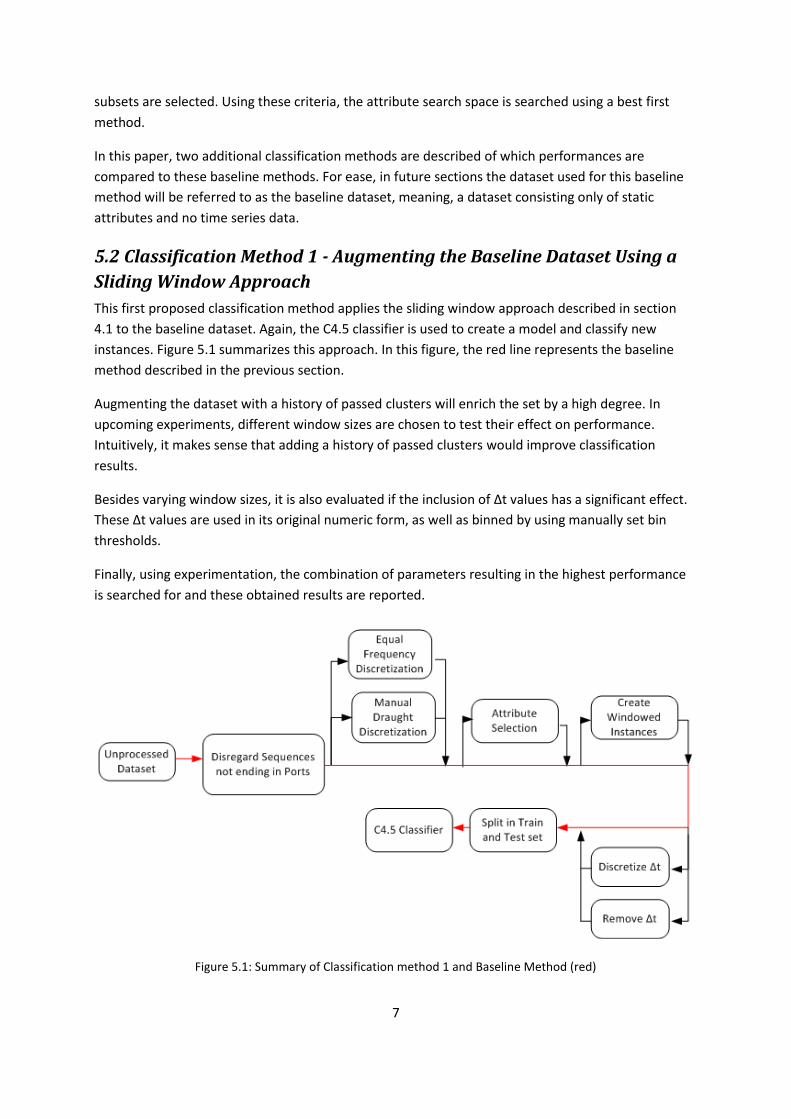
5.2 Classification Method 1 - Augmenting the Baseline Dataset Using a
Sliding Window Approach
This first proposed classification method applies the sliding window approach described in section
4.1 to the baseline dataset. Again, the C4.5 classifier is used to create a model and classify new
instances. Figure 5.1 summarizes this approach. In this figure, the red line represents the baseline
method described in the previous section.
Augmenting the dataset with a history of passed clusters will enrich the set by a high degree. In
upcoming experiments, different window sizes are chosen to test their effect on performance.
Intuitively, it makes sense that adding a history of passed clusters would improve classification
results.
Besides varying window sizes, it is also evaluated if the inclusion of ∆t values has a significant effect.
These ∆t values are used in its original numeric form, as well as binned by using manually set bin
thresholds.
Finally, using experimentation, the combination of parameters resulting in the highest performance
is searched for and these obtained results are reported.
Figure 5.1: Summary of Classification method 1 and Baseline Method (red)

8
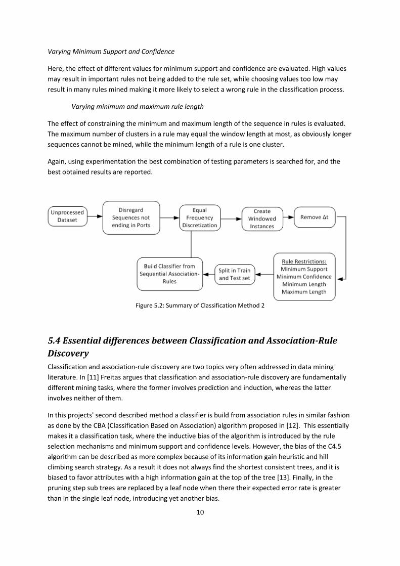
5.3 Classification Method 2 - Building a Classifier from Sequential
Association-Rules
The second approach is based on an associating mining task introduced in [9]. In this case specifically,
sequential association rules are mined from the dataset. Figure 5.2 at the end of this section
summarizes the method in a schematic overview.
Sequence mining is a method used in a variety of domains, such as shopping basket analysis and
protein sequence prediction. The goal here is to mine frequently occurring sequences (ordered
collections of items) in the dataset. An association rule is an implication in the form of X --> Y, where
this implication is satisfied in the dataset with a confidence factor 0 ≤ c ≤ 1 if and only if at least c% of
the instances of the dataset that satisfy X also satisfy Y. A sequential association-rule, is a
combination of a sequence and an association rule. By using a rule ordering system and matching the
antecedent of these rules with new instances, a classifier can be build.
The implementation of this method in this project differs from standard sequential association-rule mining tasks in that not only sequences may appear in rules, but static ship attributes as well. Therefore, resulting rules may take a form that equals a combination of a sequence and a number of ship attribute restrictions, such as: Cargo Ship, No Cargo Specified, 10, 12, 15, seg_21, poi_45 --> http://www.few.vu.nl/~wrvhage/2008/11//16/
Or, for a far less restricted example (where '_' indicates all values may be used):
_, _, _, 2, _, seg_15 --> http://www.few.vu.nl/~wrvhage/2008/11//12/
This rule refers to all ships of which their width falls in the second bin. A description of the process of
mining sequences follows:
Suppose the dataset D contains {i1, i2, .. im}, a set of m distinct items representing a cluster. An item
set or event can be described as a non empty, unordered collection of items. A sequence, however,
can be described as an ordered event. To form a sequence, items do not need to appear adjacent to
each other, as long as they are in order. To find frequent sequences in D, the basic mechanism of the
Apriori algorithm, described in [10], is used. In the first stage, D is sequentially scanned to find items
with their support being larger than the minimum support. These form the 1-sequences. These 1-
sequences are used as input for the candidate generation method to create 2-sequences. The 2-
sequences with supports larger than the threshold are collected and used as input for the 3-
sequences candidate generation method. This procedure is iteratively executed until no more non-
empty item sets can be generated.
Next, based on these sequences, we want sequential association-rules to be generated and
simultaneously to find these rules for specific ship types as well (based on type, cargo, dimensions
and draught):
For all combinations of static ship attributes, scan D and extract instances which match these
attributes. Then, perform the following steps for these instances:

9
1. Find all sequences whose support is greater than or equals the specified support threshold
using the described sequence mining method. Sequences that satisfy this condition are called
frequent sequences.
2. Generate sequential association rules based on these frequent sequences. This is
accomplished by considering all partitionings of the sequences into the antecedent A and the
consequent B of the rule. A restriction is that only a port may appear in the consequent B. The
confidence of the rule is calculated as support(AB) / support(A). When confidence meets the
required confidence threshold the rule, consisting of static attributes and a sequence
association, is added to the rule set.
Now, to select interesting rules from the dataset, constraints can be used. In this project, the
minimum support and minimum confidence constraints are used, as well as minimum and maximum
length of a rule. Because of the combination where some of the items from the instance need to be
in order and some don't, the effect of using two different minimum support measures m1 and m2 of
rule r is evaluated:
Minimum support measure m1 refers to the portion of the extracted instances that needs to
be covered by r, which will be referred to as the Relative Support
Minimum support measure m2 refers to the portion of the complete dataset that needs to be
covered by r, which will be referred to as the Absolute Support
This distinction is being made, because the distribution of ship types is not equal in the dataset. This
would result in more rules being mined for more frequently occurring ship types when exclusively
using Absolute Support.
For the classification stage, new instances are classified by matching antecedents of mined rules with
them. Here, the following rule ranking system is used:
Given two rules, ra and rb, ra precedes rb if
1. The confidence of ra is greater than that of rb
2. The confidence values of ra and rb are the same, but the support of ra is greater than that of
rb
3. The confidence and support values of ra and rb are the same, but ra has more restrictions on
the ships' static attributes, thus being more specific.
Varying Window Size
The impact of varying window sizes is measured the same way as for the first classification method.
Again, intuitively it makes sense that a history of a certain amount of clusters will yield better results.
10
Varying Minimum Support and Confidence
Here, the effect of different values for minimum support and confidence are evaluated. High values
may result in important rules not being added to the rule set, while choosing values too low may
result in many rules mined making it more likely to select a wrong rule in the classification process.
Varying minimum and maximum rule length
The effect of constraining the minimum and maximum length of the sequence in rules is evaluated.
The maximum number of clusters in a rule may equal the window length at most, as obviously longer
sequences cannot be mined, while the minimum length of a rule is one cluster.
Again, using experimentation the best combination of testing parameters is searched for, and the
best obtained results are reported.
Figure 5.2: Summary of Classification Method 2
5.4 Essential differences between Classification and Association-Rule
Discovery
Classification and association-rule discovery are two topics very often addressed in data mining
literature. In [11] Freitas argues that classification and association-rule discovery are fundamentally
different mining tasks, where the former involves prediction and induction, whereas the latter
involves neither of them.
In this projects' second described method a classifier is build from association rules in similar fashion
as done by the CBA (Classification Based on Association) algorithm proposed in [12]. This essentially
makes it a classification task, where the inductive bias of the algorithm is introduced by the rule
selection mechanisms and minimum support and confidence levels. However, the bias of the C4.5
algorithm can be described as more complex because of its information gain heuristic and hill
climbing search strategy. As a result it does not always find the shortest consistent trees, and it is
biased to favor attributes with a high information gain at the top of the tree [13]. Finally, in the
pruning step sub trees are replaced by a leaf node when there their expected error rate is greater
than in the single leaf node, introducing yet another bias.
11
Clearly, the bias of the C4.5 algorithm is a complex bias. Depending on the application domain, this
bias may fit well or it may not. Because a classifier based on association-rules lacks such complex
bias, and there is no need to use non-deterministic search methods or pruning steps, it might be
expected that the two methods produce different results.
Another theoretic difference between the two methods results from the fact that sequences can be
mined from an arbitrary long sequence, without using the windowing approach. For the decision tree
classifier however, this is not true, as this classifier requires a fixed number of attributes for every
instance. In this project however, we did use the windowing approach for the sequence miner. Not
doing so, would have resulted in sequences being mined from instances where the last cluster would
be the cluster just before ending in a port. This would actually give the system information of when a
ship is about to dock, information that is a priori not available. For this reason, for both classifiers the
windowing approach is used.
5.5 Evaluation
A widely used evaluation method for this type of classification experiment is the paired t-test on the
results of n-fold cross validation, in which the original dataset is shuffled and n folds are created.
Then, n iterations are performed where each single fold is used as test set, whereas the other n-1
folds are used as train set. Then, classification percentages of the n iterations are averaged.
A first disadvantage of this method is that different instances of the same ship would be contained in
both the test- as the train set. This method is very prone to over fitting on a specific ship, yielding
much higher results than in a realistic scenario would be achieved. This was verified by
experimentation.
A second disadvantage, pointed out by Dietterich [14], is the elevated level of Type I error, because
the method violates the independent trial assumption of the paired t-test.
A different evaluation setup is used where instead of allowing instances from a specific ship to occur
both in the train- as the test, instances marked by a specific MMSI may only occur in either of them.
Then, with this restriction, the 5 x 2 fold cross validation method described in [14] is used. In this test,
5 replications of 2-fold cross-validation are performed, where in each replication the data is
randomly split in two equal sized folds. Then, a two-tailed student T test is performed with five
degrees of freedom on the results of the 5 x 2 fold cross validation to determine any significant
differences between the methods. This method is said to have both low probability of a Type I error
and high power [14].
The results reported are the average of the classification percentages of the 5 replications.
5.6 Implementation
A testing environment is created in which all described methods can be tested and evaluated using a
graphical user interface. In this interface, all results, obtained models, mined rules etc. are reported
to the end-user in text form to allow for fast and easy testing.
All preprocessing is done by a custom created Java program. For the first classification method,
Weka´s implementations of C4.5 and attribute selection methods are used. For the second
12
classification method, our own implementation is used. The reason for using this implementation is
because the combination of rule association mining and sequential association mining is unusual, and
a free implementation was not readily available.
Running times of both classification methods are not compared to each other because faster
implementations of both classification methods are available, which would make a comparison
irrelevant. The C4.5 algorithm, for example, could be replaced by the C5.0 algorithm, which is
significantly faster [15] (only a limited version is free for use however). For the association-rule
mining method, only minor optimizations are implemented, thus making it much slower than the
C4.5 implementation. For both classification methods, however, preprocessing the dataset, creating
a classifier and classifying new instances was done in a matter of seconds. The only exception for the
second classification method would be when not discretizing the numeric ship attributes. In this case,
a vast number of attribute combinations are created, requiring an equal vast number of passes
through the dataset, resulting in very slow performance.
All testing is done on an Intel quad core system with 6 gigabytes of RAM. Multi-core is supported by
assigning each 2 fold cross-validation replica a different thread, resulting in a significant speed-up
over a single thread implementation.
6. Experimental Results Each experiment will be conducted using the earlier described 5 x 2 cross fold validation method with
the average result being reported. Experiments will be conducted for the following three categories:
Large Vessels (Tankers and Cargo Ships)
Special Crafts
Complete Dataset
Finally, to compare classification methods a student T test with five degrees of freedom is performed
to determine if differences were significant. T tests resulting in a p value of 0.05 or less are reported
as significant, denoted with an *.
6.1 Baseline Performance
Tables 6.1 and 6.2 present the results from the baseline method, and the affects of using
discretization and attribute selection methods. These can be considered variations of the baseline
method. Setting bin thresholds is accomplished by using the discretization procedure described
earlier, with the optional extension of overruling the draught bins by setting these thresholds
manually. These thresholds are acquired from a document, in which information can be found of
locations only being allowed by ships with certain draughts. For example, the Eurogeul may only be
entered by ships with a draught of 20 meters or more. From this reference document, the following
thresholds were extracted and used (in decimeters) : <143, 143 - 173, 174 - 225, >225
When using attribute selection for the complete dataset, depending on the exact train- and test set
the most often chosen attributes are type, length and draught. In case of the Large Vessel category,
length and draught are used most often. In case of the Special Crafts category only draught is chosen
as attribute, sometimes extended with the type.

13
However, in most cases, results seem to suffer from applying either of these techniques. The
exception here is for the Large Vessels category, when bin thresholds are set manually. Results
actually improve here, which makes sense as these are probably the types of vessels that have to
deal with region restrictions the most.
Large Vessels Special Crafts Complete Dataset
Baseline method 10.12 % 28.24 % 16.19 %
Automatic Binning 11.40 % 23.36 % 9.81 %
Manual Draught Bins 14.80 % 23.70 % 13.50 %
Table 6.1: Using Bins (percentage of correct classifications)
Large Vessels Special Crafts Complete Dataset
Baseline method 10.12 % 28.24 % 16.19 %
Attribute Selection 10.27 % 26.06 % 12.82
Table 6.2: Using Attribute Selection (percentage of correct classifications)
For two out of three categories the baseline method performs best when not using any discretization
or attribute selection methods. For that reason, in upcoming sections, performance of the presented
classification methods are compared to this standard baseline method.
6.2 Experiment 1
Using the first described classification method, experiments are conducted to evaluate this method.
In figure 6.1, the results of using the sliding window approach can be seen compared to those of the
baseline performance. For all three categories, up to a certain window size, classification percentages
improve. After that point, results more or less stay the same, or even decrease somewhat.
Apparently, to increase accuracy different windows sizes should be chosen for different ship types.
For example, in case of the Special Crafts category, it does not make much sense to use a window
size larger than 2. For the Large Vessels category however, an improvement can be seen in accuracy
even when increasing window size from 3 to 4.
14
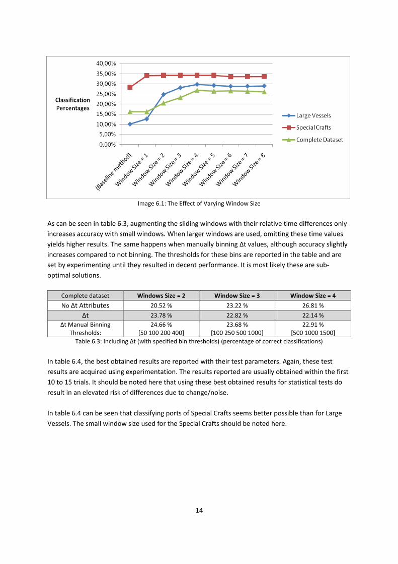
Image 6.1: The Effect of Varying Window Size
As can be seen in table 6.3, augmenting the sliding windows with their relative time differences only
increases accuracy with small windows. When larger windows are used, omitting these time values
yields higher results. The same happens when manually binning ∆t values, although accuracy slightly
increases compared to not binning. The thresholds for these bins are reported in the table and are
set by experimenting until they resulted in decent performance. It is most likely these are sub-
optimal solutions.
Complete dataset Windows Size = 2 Window Size = 3 Window Size = 4
No ∆t Attributes 20.52 % 23.22 % 26.81 %
∆t 23.78 % 22.82 % 22.14 %
∆t Manual Binning Thresholds:
24.66 % [50 100 200 400]
23.68 % [100 250 500 1000]
22.91 % [500 1000 1500]
Table 6.3: Including ∆t (with specified bin thresholds) (percentage of correct classifications)
In table 6.4, the best obtained results are reported with their test parameters. Again, these test
results are acquired using experimentation. The results reported are usually obtained within the first
10 to 15 trials. It should be noted here that using these best obtained results for statistical tests do
result in an elevated risk of differences due to change/noise.
In table 6.4 can be seen that classifying ports of Special Crafts seems better possible than for Large
Vessels. The small window size used for the Special Crafts should be noted here.

15
Large Vessels Special Crafts Complete Dataset
(Baseline method) 10.12 % 28.24 % 16.19 %
Best Results 29.97 % Window Size = 4 Discretize (automatic)
No ∆t attributes
35.24 % Window Size = 1 Discretize (automatic)
No ∆t attributes
26.81 % Window Size = 4
No ∆t attributes
Significance Level * t = 12.2517 p < 0.0001
* t = 4.1248 p = 0.0091
* t = 8.6686 p = 0.0003
Table 6.4: Best Obtained Results (percentage of correct classifications)
For all three categories the T-test resulted in P values of less than 0.05, thus concluding that the
proposed method performs significantly better than the baseline method.
6.3 Experiment 2
In this second experiment the second classification method is tested. The same approach is taken as
in the first experiment, were 5x2 cross-fold validation will be performed and the average of the
results are reported.
A side note is that the following experiments are almost exclusively performed with the discretization
parameter set to true. As for each possible combination of static ship attributes rules are mined, this
would otherwise result in a vast number of rules being mined for a vast number of combinations of
ship attributes. This proved to be computationally too expensive.
Min. Confidence = 0.5 Window Size = 1
Relative Support Absolute Support
Min support = 0.1 2.64 % 0.0 %
Min support = 0.01 21.32 % 5.63 %
Min support = 0.001 24.66 % 22.52 %
Min support = 0.0005 24.78 % 24.78 %
Table 6.5: Different Levels of Minimum Support (percentage of correct classifications)
It seems that lowering support yields better results, as demonstrated in table 6.5. For both types of
support levels, values set this low results in every candidate rule being added to the rule set.
Therefore, choosing one minimum support measure over the other does not yield better results.
From now on, only the relative support measure is used.
Min. Support = 0.0005 Window Size = 1
Complete Dataset
Min Confidence = 0.5 24.78 %
Min Confidence = 0.4 25.97 %
Min Confidence = 0.3 26.21 %
Min Confidence = 0.2 26.25 %
Table 6.6: Different Values of Minimum Confidence (percentage of correct classifications)

16
In table 6.6 minimum confidence levels are evaluated, where the minimum support is set to 0.0005.
When lowering minimum confidence we can see the same effect happening as when lowering
minimum support: performance increases along with lowering minimum confidence up to a certain
point (in this case 0.2).
Figure 6.2 : The Effect of Varying Window Size
Figure 6.2 shows the results of augmenting the dataset with sliding windows, where minimum
support and confidence levels are respectively set to 0.0005 and 0.2. Again, augmenting the dataset
with sliding windows increases accuracy. Compared to the C4.5 classification method however,
results seem to stabilize earlier when increasing window size. The results demonstrated in table 6.7,
where different constraints on sequence length are used, confirm this by showing that most
important rules consist of 1-sequences and 2-sequences. Like for the minimum support and
confidence levels, it should be noted that classification percentages improve when less restrictions
are placed (in this case using 1,2 and 3-sequences).
Min Support = 0.0005 Min Confidence = 0.2
Length 1 - 1 Length 1 - 2 Length 2 - 2 Length 2 - 3 Length 1 - 3 Length 3 - 3
Complete Dataset 25.43 % 25.85 % 19.11 % 19.19% 25.92 % 11.46 %
Table 6.7: Evaluating Length of Mined Sequences (percentage of correct classifications)
The best obtained results are reported in table 6.8 along with their testing parameters. For
comparison, the best obtained results of the first classification method are presented here as well. A
summary of the significance levels are presented in table 6.9.
Large Vessels Special Crafts Complete Dataset
Baseline method 10.12 % 28.24 % 16.19 %
Best Results M1 29.97 % 35.24 % 26.81 %
Best Results M2 27.27% Window Size = 2 Min. Support = 0.0005 Min. Confidence = 0.2
34.67% Window Size = 2 Min. Support = 0.0005 Min. Confidence = 0.2
26.54 % Window Size = 2 Min. Support = 0.0005 Min. Confidence = 0.2
Table 6.8: Best Obtained Results Methods 1 & 2 (percentage of correct classifications)

17
Large Vessels Special Crafts Complete Dataset
Baseline method <--> Best Result M1
* t = 12.2517 p < 0.0001
* t = 4.1248 p = 0.0091
* t = 8.6686 p = 0.0003
Baseline method <--> Best Results M2
* t = 11.0472 p = 0.0001
* t = 2.6952 p = 0.0430
* t = 11.3586 p < 0.0001
Best Results M1 <--> Best Results M2
* t = 4.3185 p = 0.0076
t = 0.3793 p = 0.7200
t = 0.1746 p = 0.8682
Table 6.9: Summary of Significance Levels
In all three categories the second proposed classification method outperforms the baseline method
with a significant difference. When comparing the first method with the second method however,
these results are closer. Only for the Large Vessels category is there a significant difference, in favor
of the C4.5 method.
Compared to the size of the generated trees for the complete dataset (about 3000-5000 leaves) and
the Large Vessels category (2500-3500 leaves), the size of the generated tree for the Specials Crafts is
particularly small (about 100 to 200 leaves). Most of these trees contain the 'type' attribute at the
root of the tree. Furthermore, most extracted rules from the trees contain passed clusters.
For the second classification method, rule sets contain many more rules. Again, for the Special Crafts
the least number of rules are generated (6000-7000), followed by the Large Vessels (about 30.000)
and the complete dataset (about 50.000).
As explained earlier, up to now binning has been used to reduce computational costs. However, if
the trend continues where more rules in the rule set result in higher performance, we should be
seeing some improvements when not using any discretization as well. Table 6.10 presents the results
of an experiment where for two categories the performance is compared between using
discretization and not using discretization. Accuracy does improve, and as a result this method
outperforms the best obtained results of the first classification method for the Special Crafts
category. Unfortunately, mining the complete dataset without using any bins was computationally to
expensive. It would be interesting to see more extensive testing results performed by a more
efficient implementation.
Window Size = 1 Window Size = 2 Window Size = 3
Special Crafts - No Binning 32.91 % 34.67 % 34.07 %
Special Craft - Binning 35.36 % 36.56 % 35.23 %
Large Vessels - No Binning 26.84 % 27.27 % 26.46 %
Large Vessels - Binning 28.21 % 27.52 % 26.90 %
Table 6.10 : Using bins or no bins (percentage of correct classifications)
6.4 Experiment 3
In this third experiment, the classification attribute is changed from the final port to the next cluster.
In other words, a location less distant into the future is predicted. The same classification methods as
in the first two experiments are used. As for the data-preprocessing, instances are created by using
the same sliding window approach as in the previous experiments. This time, however, all data is
18
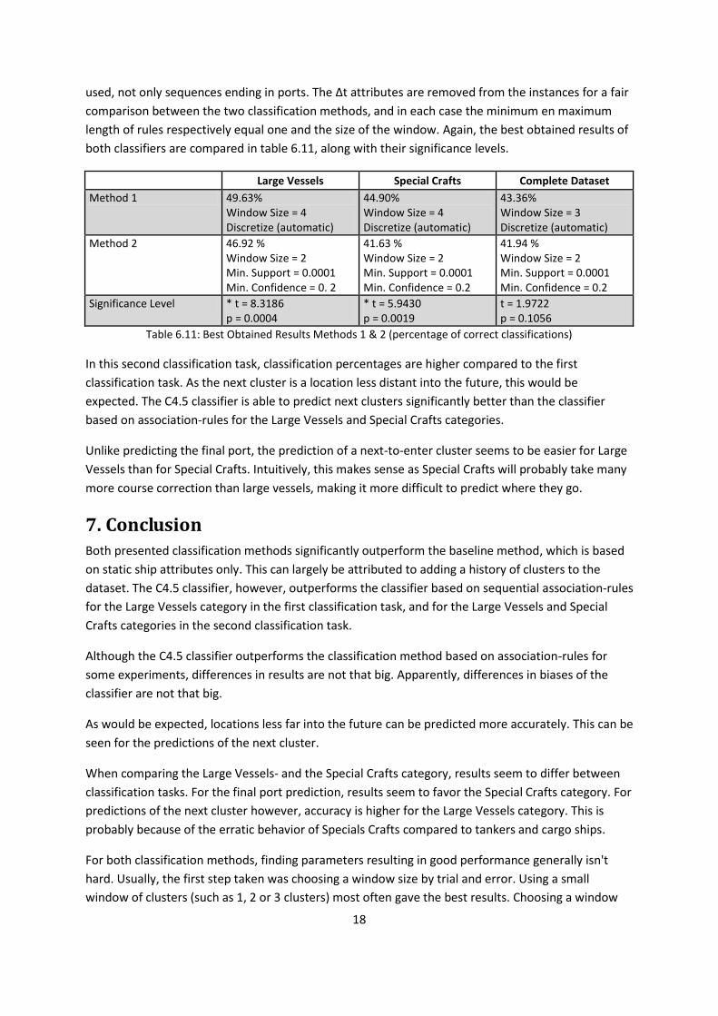
used, not only sequences ending in ports. The ∆t attributes are removed from the instances for a fair
comparison between the two classification methods, and in each case the minimum en maximum
length of rules respectively equal one and the size of the window. Again, the best obtained results of
both classifiers are compared in table 6.11, along with their significance levels.
Large Vessels Special Crafts Complete Dataset
Method 1 49.63% Window Size = 4 Discretize (automatic)
44.90% Window Size = 4 Discretize (automatic)
43.36% Window Size = 3 Discretize (automatic)
Method 2 46.92 % Window Size = 2 Min. Support = 0.0001 Min. Confidence = 0. 2
41.63 % Window Size = 2 Min. Support = 0.0001 Min. Confidence = 0.2
41.94 % Window Size = 2 Min. Support = 0.0001 Min. Confidence = 0.2
Significance Level * t = 8.3186 p = 0.0004
* t = 5.9430 p = 0.0019
t = 1.9722 p = 0.1056
Table 6.11: Best Obtained Results Methods 1 & 2 (percentage of correct classifications)
In this second classification task, classification percentages are higher compared to the first
classification task. As the next cluster is a location less distant into the future, this would be
expected. The C4.5 classifier is able to predict next clusters significantly better than the classifier
based on association-rules for the Large Vessels and Special Crafts categories.
Unlike predicting the final port, the prediction of a next-to-enter cluster seems to be easier for Large
Vessels than for Special Crafts. Intuitively, this makes sense as Special Crafts will probably take many
more course correction than large vessels, making it more difficult to predict where they go.
7. Conclusion Both presented classification methods significantly outperform the baseline method, which is based
on static ship attributes only. This can largely be attributed to adding a history of clusters to the
dataset. The C4.5 classifier, however, outperforms the classifier based on sequential association-rules
for the Large Vessels category in the first classification task, and for the Large Vessels and Special
Crafts categories in the second classification task.
Although the C4.5 classifier outperforms the classification method based on association-rules for
some experiments, differences in results are not that big. Apparently, differences in biases of the
classifier are not that big.
As would be expected, locations less far into the future can be predicted more accurately. This can be
seen for the predictions of the next cluster.
When comparing the Large Vessels- and the Special Crafts category, results seem to differ between
classification tasks. For the final port prediction, results seem to favor the Special Crafts category. For
predictions of the next cluster however, accuracy is higher for the Large Vessels category. This is
probably because of the erratic behavior of Specials Crafts compared to tankers and cargo ships.
For both classification methods, finding parameters resulting in good performance generally isn't
hard. Usually, the first step taken was choosing a window size by trial and error. Using a small
window of clusters (such as 1, 2 or 3 clusters) most often gave the best results. Choosing a window
19
size too big often resulted in worse performance. This can probably be attributed to the classifiers
not being able to handle the large number of attributes very well, a problem in classification tasks
often referred to as the 'Curse of Dimensionality'. Besides choosing an appropriate window size, for
the C4.5 classifier the exclusion of ∆t attributes seemed to be the only parameter significantly
improving classification accuracy. Again, this is probably a results of the classifier not being able to
handle the extra attributes very well. Using discretization didn´t make matters any better here.
For both classification tasks, it is hard to say if classification accuracy is high to enough to use such
classification method in practice. One reason for this is that without a more in depth analysis of the
results there is no information for which ship types, clusters, ports, etc. predictions can be
considered good. As presented results are averaged classification percentages, these results may for
example mask specific locations for which accuracy is a lot better. The same could be the case for
specific ship types, ships with a certain cargo, etc.
8. Future Work Most importantly, future research should focus on the analysis of the obtained results in this paper
(e.g. the results of different cluster plotted on a geographic map). Without knowing in which
situations and for what reasons these methods fail to predict future locations, it becomes hard to
efficiently implement any improvements.
However, some straightforward improvements include the use of different learning algorithms, as
well as different discretization- and attribute selection methods. Also, the effect of augmenting the
dataset with other attributes could be measured. These could be attributes contained in the AIS data
(such as navigational status, rate of turn, destination, etc.), or these could be external attributes like
weather conditions, day of the week, etc. Furthermore, it would be interesting to see if a larger
dataset yields different results.
To reduce the currently vast number of association rules mined from the dataset, pruning methods
could be employed.
As association rules allow multiple items in the consequent, another possibility is that a model could
be build where a sequence of future events is predicted by one rule, instead of just one future event
(which is the case for final port or next cluster). Also, instead of predicting future events, based on
the history of passed clusters static ship attributes could be predicted in case this information is
missing.
Finally, attention could be paid to creating models that detect anomalies. This way coast guard
operators can be alarmed in time if something unexpected happens. For example, this could be a
ship on a collision course, or an unauthorized entrance of a region by a ship. This would probably
improve situational awareness.

20
9. References [1] G. de Vries and M. van Someren, "Unsupervised Ship Trajectory Modeling and Prediction Using
Compression and Clustering", In BNAIC 2008, Proceedings 20th Belgian-Netherlands Conference
on Artificial Intelligence
[2] D. Douglas and T. Peucker, "Algorithms for the reduction of the number of points required to
represent a digitized line or its caricature.", The Canadian Cartographer, 10(2):112–122, 1973
[3] D. Lindsay and S. Cox, "Effective Probability Forecasting for Time Series Data Using Standard Machine Learning Techniques", in Lecture Notes in Computer Science, Volume 3686 (2005) [4] Y. Yang and G.I. Webb, "A comparative study of discretization methods for naïve-bayes classifiers", Proceeding of the Pacific Rim Knowledge Acquisition Workshop, 2002. [5] J. R. Quinlan. "C4.5: Programs for Machine Learning", Morgan Kaufmann, 1993.
[6] G. Batista and M.C. Monard, "An Analysis of Four Missing Data Treatment Methods for Supervised Learning", Applied Artificial Intelligence, 17: 519–533, 2003 [7] J. Dougherty, R. Kohavi and M. Sahami, "Supervised and Unsupervised Discretization of Continuous Features", In Prieditis, A., & Russell, S. (Eds.), Proceedings of the Twelfth International Conference on Machine Learning, pp. 194–202, (1995) San Francisco. Morgan Kaufmann [8] M. Hall, "Feature Subset Selection: A correlation Based Filter Approach", in Proc. Fourth International Conference on Neural Information Processing and Intelligent Information Systems, pp 855-858, 1997 [9] R. Agrawal, T. Imielinski, and A. Swami, "Mining Association Rules Between Sets of Items in Large Databases", ACM SIGMOD Conf. Management of Data, May 1993
[10] R. Agrawal, R. Srikant, “Fast algorithm for mining association rules”, Proc. of 20th VLDB, pp.487- 499, 1994 [11] A.A. Freitas, "Understanding the crucial differences between classification and discovery of association rules - a position paper", To appear in ACM SIGKDD Explorations, 2(1), 2000 [12] B. Liu, W. Hsu, and Y. Ma, “Integrating classification and association rule mining.” KDD-98, New York, 1998 [13] T Mitchell, "Machine Learning", McGraw Hill, pp 63-72, 1997 [14] T.G. Dietterich, "Approximate statistical tests for comparing supervised classification learning algorithms', Neural Computation, 1998, 10:1885-1924 [15] http://www.rulequest.com/see5-comparison.html