leach-sm: a protocol for extending wireless sensor …
TRANSCRIPT

Western Michigan University Western Michigan University
ScholarWorks at WMU ScholarWorks at WMU
Dissertations Graduate College
1-2011
LEACH-SM: A Protocol for Extending Wireless Sensor Network LEACH-SM: A Protocol for Extending Wireless Sensor Network
Lifetime by Management of Spare Nodes Lifetime by Management of Spare Nodes
Bilal Abu Bakr Western Michigan University
Follow this and additional works at: https://scholarworks.wmich.edu/dissertations
Part of the Computer Engineering Commons, and the Computer Sciences Commons
Recommended Citation Recommended Citation Bakr, Bilal Abu, "LEACH-SM: A Protocol for Extending Wireless Sensor Network Lifetime by Management of Spare Nodes" (2011). Dissertations. 344. https://scholarworks.wmich.edu/dissertations/344
This Dissertation-Open Access is brought to you for free and open access by the Graduate College at ScholarWorks at WMU. It has been accepted for inclusion in Dissertations by an authorized administrator of ScholarWorks at WMU. For more information, please contact [email protected].

LEACH-SM: A PROTOCOL FOR EXTENDING WIRELESS SENSOR NETWORK
LIFETIME BY MANAGEMENT OF SPARE NODES
by
Bilal Abu Bakr
A Dissertation Submitted to the
Faculty of The Graduate College in partial fulfillment of the
requirements for the Degree of Doctor of Philosophy
Department of Computer Science Advisor: Leszek T. Lilien, Ph.D.
Western Michigan University Kalamazoo, Michigan
June 2011
LEACH-SM: A PROTOCOL FOR EXTENDING WIRELESS SENSOR NETWORK LIFETIME BY MANAGEMENT OF SPARE NODES
Bilal Abu Bakr, Ph.D.
Western Michigan University, 2011
Operational lifetime of a wireless sensor network (WSN) depends on its energy
resources. Significant improvement of WSN lifetime can be achieved by adding spare
sensor nodes to WSN. Spares are ready to be switched on when any primary (a node that
is not a spare) exhausts its energy. A spare replacing a primary becomes a primary itself.
The LEACH-SM protocol (Low-Energy Adaptive Clustering Hierarchy with
Spare Management) proposed by us is a modification of the prominent LEACH protocol.
LEACH extends WSN lifetime via rotation of cluster heads but allows for inefficiencies
due to redundant sensing target coverage. There are two energy-consumption
inefficiencies in LEACH. The first one, the hotspot problem, is due to extra duties of
cluster heads (as compared to regular nodes) that increase their energy usage. The second
inefficiency is redundant data transmissions to cluster heads (made by regular nodes
covering targets redundantly). Both inefficiencies are reduced by using spares in
LEACH-SM.
LEACH-SM has three main features. First, from the subset of WSN nodes that
provide redundant area coverage, we select the optimal collection of spares (to maximize
extension of WSN lifetime). We overcome race conditions and deadlocks that can occur

during the spare selection process. The second main feature is deciding how long spares
should remain asleep, and which spares should be used as replacements for primaries that
exhausted their energy. The third main feature is estimating WSN lifetime as determined
by energy consumption of all its sensor nodes.
We provided analytical estimates and comparisons of LEACH and LEACH-SM
for simplified cases. We also run simulation experiments (using MATLAB) to compare
both protocols for general and complex cases. We studied the impact of the spare ratio
and duration of the nap interval of cluster heads on the WSN lifetime for LEACH and
LEACH-SM.
Even when no spares are used, LEACH-SM achieves 23% to 48% extension of
the average WSN lifetime when compared to LEACH (this is due to switching off
redundant nodes in LEACH-SM). When LEACH-SM uses spares, LEACH-SM achieves
183% extension of the average WSN lifetime when compared to LEACH (which is
unable to use spares).

All rights reserved
INFORMATION TO ALL USERSThe quality of this reproduction is dependent on the quality of the copy submitted.
In the unlikely event that the author did not send a complete manuscriptand there are missing pages, these will be noted. Also, if material had to be removed,
a note will indicate the deletion.
All rights reserved. This edition of the work is protected againstunauthorized copying under Title 17, United States Code.
ProQuest LLC.789 East Eisenhower Parkway
P.O. Box 1346Ann Arbor, MI 48106 - 1346
UMI 3471047
Copyright 2011 by ProQuest LLC.
UMI Number: 3471047

Copyright by Bilal Abu Bakr
2011

Dedicated to my father Prof. Irshad Ul Hasan

ii
ACKNOWLEDGMENTS
All praise to Almighty Allah for granting me perseverance to carry my research to
fruitful completion. It was a fascinating enterprise to move from the known through the
less known to the unknown aspects of the subject of my research. It was a cruise, an
academic expedition to enlarge the frontiers of knowledge within the chosen specific
framework. It involved visualization, conceptualization, and organization of data to arrive
at concrete and verifiable results. As I proceeded with my research with quantifiable
approach, I went on scaling one promontory after another.
I appreciate Prof. Leszek Lilien’s dedication to the widening of horizons. I cherish
my interaction with him to gain new insights. I marshaled my findings and tested them
before formulating them in the form of my Thesis work.
I would like to extend my sincere gratitude to Professor Ajay Gupta who
continuously shared his insights in the research subject and provided me with his
analyses and scientific critique of the underlying concept of my research project.
I greatly value the support of my Thesis committee members Professors Elise de
Doncker, and Ikhlas Abdel-Qader. I would like to thank them all for their valuable
comments, discussions, and suggestions during all stages of my work on this Thesis.
I am also so grateful to the faculty and staff of the Department of Computer
Science for helping me during this academic exploration and quest. My special thanks go
to the Department Chair, Prof. Donald Nelson; the faculty: Professors Dionysios
Kountanis, Ala Al-Fuqaha, Mark Kerstetter, and Ron Miller; and the department staff
Natallie Bolliger, John Horton, and Sheryl Todd.

iii
Acknowledgments – Continued
I would like also to thank my colleagues and library staff friends for their help
and support in the course of this research thesis.
Thanks are also due to my parents who constantly remember me in their prayers,
particularly my mother who initiated me into love and fear of God and planted in me
insatiable thirst for knowledge.
Finally, I would like to thank my wonderful wife. She has kept me happy and
stable during the Ph.D. process, and I thank her for all her tolerance and her never-ending
optimism when I came home late, frustrated, and stressed.
Bilal Abu Bakr

iv
TABLE OF CONTENTS
ACKNOWLEDGMENTS ................................................................................. ii
LIST OF TABLES ............................................................................................. xi
LIST OF FIGURES ........................................................................................... xii
CHAPTER
1. INTRODUCTION TO THE PROBLEM .............................................. 1
1.1 Using Redundancy for Extending WSN Lifetime ........................ 3
1.2 Motivation ..................................................................................... 3
1.3 Outline of the Proposed Solution: The LEACH-SM Protocol ......................................................................................... 4
1.4 Organization.................................................................................. 7
2. BACKGROUND INFORMATION ...................................................... 8
2.1 Deployment of Wireless Sensor Nodes and Object Coverage ....................................................................................... 9
2.2 Object Coverage and Connectivity ............................................... 10
2.3 Definition of SR-neighbor ............................................................ 12
2.4 Power Modes for Wireless Sensor Nodes..................................... 12
2.5 The Duty Cycle for WSN Nodes .................................................. 13
2.6 WSN Failures and Battery Capacity ............................................. 14
3. RESEARCH GOALS ............................................................................ 16
3.1 Goal 1: Optimal Spare Selection .................................................. 16
3.2 Goal 2: Management of Spare Nodes after WSN Deployment ................................................................................... 17

v
Table of Contents—Continued
CHAPTER
3.3 Goal 3: Estimating the Lifetime of WSN ..................................... 18
4. RELATED WORK ................................................................................ 19
5. DETAILED ANALYSIS OF THE INEFFICIENCY PROBLEM IN LEACH ......................................................................... 25
5.1 Timeline of LEACH ..................................................................... 26
5.2 The Inefficiency in LEACH ......................................................... 27
5.3 Notation ........................................................................................ 29
5.4 Calculating Duration of Awake Interval for LEACH ................... 33
5.4.1 Duration of Awake Interval for Regular Sensor Nodes ................................................................................... 34
5.4.2 Duration of Awake Interval for Cluster Head ..................... 35
5.4.3 Duration of Nap Interval for Cluster Head ......................... 37
5.5 Calculating Duty Cycle for LEACH ............................................. 37
5.5.1 Case 1: Duration of Nap Interval for Cluster Head is Zero ........................................................................ 38
5.5.1.1 Calculating the Duty Cycle for Cluster Head ........................................................................ 38
5.5.1.2 Calculating the Duty Cycle for Regular Nodes ...................................................................... 38
5.5.2 Case 2: Duration of Nap Interval for Cluster Head is Not Zero ................................................................. 39
5.5.2.1 Calculating the Duty Cycle for Cluster Head ........................................................................ 39
5.5.2.2 Calculating the Duty Cycle of Regular Nodes ...................................................................... 39

vi
Table of Contents—Continued
CHAPTER
5.6 Energy Consumption Model for LEACH ..................................... 39
5.6.1 Average Current Drawn by Regular Nodes ........................ 40
5.6.2 Average Current Drawn by Cluster Heads .......................... 40
5.7 Special-case Calculation of WSN Lifetime for LEACH ......................................................................................... 41
5.8 Calculating WSN Lifetime for LEACH-C and LEACH-F...................................................................................... 46
5.9 Residual WSN Lifetime for LEACH and its Variants .................. 46
6. LEACH-SM – THE PROPOSED SOLUTION TO THE LEACH INEFFICIENCY PROBLEM .................................................. 48
6.1 Cluster Setup Phase of LEACH-SM ............................................. 48
6.2 Spare Selection Phase of LEACH-SM ......................................... 49
6.2.1 Interval 1: Sensing Range Neighbor Discovery .................. 49
6.2.2 Interval 2: Running the Decentralized Energy-efficient Spare Selection Technique (DESST) .................... 52
6.2.2.1 Finding the Order of Nodes for Making the Primary/Spare Decision .................................... 55
6.2.2.2 Primary/Spare Decision .......................................... 58
6.2.2.3 Example 1: SR-neighbor Discovery (Output of Algorithm 1) .......................................... 63
6.2.2.4 Example 2: Nodes Making the Spare/Primary Decision (Output of Algorithm 2) ........................................................... 72

vii
Table of Contents—Continued
CHAPTER
7. MANAGEMENT AND SCHEDULING OF SPARE SENSOR NODES .................................................................................. 79
7.1 Management of Redundant Sensor Nodes .................................... 79
7.2 Selecting Spares ............................................................................ 80
7.3 Scheduling Spares ......................................................................... 80
7.4 The State Diagram for Nodes During Execution of LEACH-SM .................................................................................. 83
8. ANALYTICAL COMPARISON OF WSN LIFETIME FOR LEACH AND LEACH-SM .......................................................... 86
8.1 Timeline of LEACH-SM .............................................................. 86
8.2 Calculating Duration of Awake Interval for LEACH-SM ................................................................................................. 87
8.2.1 Duration of Awake Interval for Regular Sensor Nodes ................................................................................... 87
8.2.2 Duration of Awake Interval for Cluster Head ..................... 87
8.2.3 Duration of Nap Interval for Cluster Head ......................... 90
8.3 Calculating the Duty Cycle for LEACH-SM ................................ 91
8.3.1 Case 1: Duration of Nap Interval for Cluster Head is Zero ........................................................................ 91
8.3.1.1 Calculating the Duty Cycle for Cluster Head ........................................................................ 91
8.3.1.2 Calculating the Duty Cycle for Regular Nodes ...................................................................... 92
8.3.1.3 Calculating the Duty Cycle for Spare Nodes ...................................................................... 92

viii
Table of Contents—Continued
CHAPTER
8.3.2 Case 2: Duration of Nap Interval for Cluster Head is Not Zero ................................................................. 92
8.3.2.1 Calculating the Duty Cycle for Cluster Head ........................................................................ 92
8.3.2.2 Calculating the Duty Cycle for Regular Nodes ...................................................................... 92
8.3.2.3 Calculating the Duty Cycle for Spare Nodes ...................................................................... 93
8.4 Energy Consumption Model for LEACH-SM .............................. 93
8.4.1 Average Current Drawn by Regular Nodes ........................ 93
8.4.2 Average Current Drawn by Cluster Heads .......................... 93
8.4.3 Average Current Drawn by Spares ..................................... 94
8.5 Special-case Calculation of WSN Lifetime for LEACH-SM .................................................................................. 94
8.6 Spare Lifetime and Residual Spare Lifetime in LEACH-SM .................................................................................. 95
8.7 Residual WSN Lifetime for LEACH-SM ..................................... 96
9. SIMULATION OF LEACH AND LEACH-SM ................................... 97
9.1 Simulation Description ................................................................. 97
9.1.1 Simulation Scenarios ........................................................... 98
9.1.2 Simulation Models .............................................................. 100
9.1.2.1 Energy Consumption Model ................................... 100
9.1.2.2 Model for Number of Frames Per Round ...................................................................... 101

ix
Table of Contents—Continued
CHAPTER
9.2 Metrics .......................................................................................... 101
9.3 Simulation Assumptions ............................................................... 102
9.4 Simulation Setup ........................................................................... 102
9.4.1 Input Parameters .................................................................. 102
9.4.2 Random Variables ............................................................... 105
9.5 Simulation Results ........................................................................ 107
9.5.1 Results of Energy Consumption and WSN Lifetime Simulations for LEACH and LEACH-SM without Spare Replacements ........................................ 107
9.5.1.1 Simulation Results for Individual Combinations of and α Values ........................ 108
9.5.1.2 Simulation Results for Ranges of or α Values ...................................................... 133
9.5.2 Results of Energy Consumption and WSN Lifetime Simulations for LEACH-SM with Spare Replacements ............................................................ 147
9.5.2.1 Simulation Results for Individual Combinations of and α Values ........................ 148
9.5.2.2 Simulation Results for Ranges of or α Values ...................................................... 163
9.6 Simulation Conclusions ................................................................ 166
10. CONCLUSIONS.................................................................................... 168
10.1 Summary ....................................................................................... 168
10.2 Contributions ................................................................................ 170
10.3 Future Work .................................................................................. 171

x
Table of Contents—Continued
CHAPTER
APPENDIX A .............................................................................................. 172
BIBLIOGRAPHY ........................................................................................ 196

xi
LIST OF TABLES
5.1. Notation .................................................................................................... 29
9.1. Simulated combinations of values for and .................................... 99
9.2. Input parameters. ...................................................................................... 103
9.3. Random variables and their statistical properties. .................................... 106
9.4. Comparison of LEACH-SM with LEACH. ............................................. 108
9.5. Comparison of LEACH-SM with LEACH. ............................................. 134
9.6. Cases to measure WSN lifetime when replacements of exhausted primary nodes by spares are allowed. ..................................... 152
9.7. LEACH-SM with one replacement. ......................................................... 164
9.8. Average WSN lifetime for a single node for LEACH and LEACH-SM. ............................................................................................ 166

xii
LIST OF FIGURES
1.1. Rounds, phases, and frames for LEACH-SM, including the added spare selection phase.. .................................................................... 6
2.1. Hardware components of a typical sensor node. ...................................... 8
2.2. Irregular shape for transmission and sensing ranges. ............................... 10
2.3. State diagram for power modes of sensor nodes. ..................................... 13
2.4. Basic frame structure for sensor nodes. ................................................... 13
4.1. Three main categories of solutions extending WSN lifetime. ................. 19
5.1. Rounds, phases, and frames for one cluster (with a cluster head and nc regular nodes) in LEACH. ................................................... 25
5.2. Timing of awake and nap intervals for a cluster head and its 1 regular nodes. ............................................................................... 27
5.3. Different periods within a frame for a cluster head and regular nodes in LEACH. ......................................................................... 34
6.1. Rounds, phases, and frames for LEACH-SM, including the added spare selection phase.. .................................................................... 48
6.2. Illustration for SR-neighbor discovery. .................................................... 50
6.3. The SNR tables for four nodes after the hello—hello-reply message exchanges by them. ..................................................... 51
6.4. DESST puts each WSN node into either passive or active power mode. ............................................................................................. 52
6.5. Pseudocode of Algorithm 1 in DESST. ................................................... 54
6.6. The SRN tables for , , ,and after applying Algorithm 1. ............................................................................................. 56
6.7. The order in which nodes , , ,and must make the spare/primary decision. ............................................................................ 57

xiii
List of Figures—Continued
6.8. Pseudocode of Algorithm 2 in DESST. ................................................... 58
6.9. The node becomes a spare and switched into passive mode, estimated by DESST during the spare selection phase. ................ 60
6.10. The node becomes a primary and switched into active mode, estimated by DESST during the spare selection phase. ................ 62
6.11. Illustration for Example 1 of SR-neighbor discovery. ............................. 63
6.12. Illustration of sending and receiving of a hello message. .................... 64
6.13. SRN table for node 2 (below target A). ................................................... 65
6.14. Sorted SRN tables for all nodes. .............................................................. 70
6.15. The order in which node makes the spare/primary decision. .................................................................................................... 71
6.16. The order in which node makes the spare/primary decision. .................................................................................................... 72
6.17. The node becomes a spare (switches into passive mode) as decided by DESST during the spare selection phase. .............................. 74
6.18. The node becomes a spare as decided by DESST. .............................. 75
6.19. The node becomes a spare. ................................................................. 76
6.20. Illustration of selecting primary/spare status. .......................................... 77
6.21. The frame structure and timing of frame components for cluster heads in LEACH and LEACH-SM. ............................................. 78
7.1. Awake/Nap cycles for primaries and spares in LEACH-SM. .................. 81
7.2. Duty cycle of active and spare nodes in LEACH-SM, in which the spares follow the Awake/Nap cycle from time t. .................... 82
7.3. The replacement process for a primary that exhausted its energy. ...................................................................................................... 83

xiv
List of Figures—Continued
7.4. The state diagram for nodes states during execution of LEACH-SM. ............................................................................................ 84
8.1. Rounds, phases, and frames for LEACH-SM, including the added spare selection phase. ..................................................................... 86
8.2. Timing of awake and nap intervals for a cluster head and its 1 1 regular nodes. ............................................................... 88
8.3. Timeline of activities for each type of sensor node in LEACH-SM. ............................................................................................ 89
8.4. Comparison of cluster head activities in LEACH and LEACH-SM. ............................................................................................ 90
9.1. Twenty individual energy consumption curves and twenty individual WSN lifetimes for a single node for LEACH and for LEACH-SM with 0 and 25% (based on 20 simulation runs). ....................................................................................... 110
9.2. Average energy consumption curves and average WSN lifetimes for a single node for LEACH and LEACH-SM with
0 and 25% (based on 20 simulation runs). ........................... 111
9.3. Twenty individual energy consumption curves and twenty individual WSN lifetimes for a single node for LEACH and for LEACH-SM with 0 and 50% (based on 20 simulation runs). ....................................................................................... 113
9.4. Average energy consumption curves and average WSN lifetimes for a single node for LEACH and LEACH-SM with
0 and 50% (based on 20 simulation runs). ........................... 114
9.5. Twenty individual energy consumption curves and twenty individual WSN lifetimes for a single node for LEACH and for LEACH-SM with 10 and 25% (based on 20 simulation runs). ....................................................................................... 116
9.6. Average energy consumption curves and average WSN lifetimes for a single node for LEACH and LEACH-SM with
10 and 25% (based on 20 simulation runs). ......................... 117

xv
List of Figures—Continued
9.7. Twenty individual energy consumption curves and twenty individual WSN lifetimes for a single node for LEACH and for LEACH-SM with 10 and 50% (based on 20 simulation runs). ....................................................................................... 119
9.8. Average energy consumption curves and average WSN lifetimes for a single node for LEACH and LEACH-SM with
10 and 50% (based on 20 simulation runs). ......................... 120
9.9. Twenty individual energy consumption curves and twenty individual WSN lifetimes for a single node for LEACH and for LEACH-SM with 20 and 25% (based on 20 simulation runs). ....................................................................................... 122
9.10. Average energy consumption curves and average WSN lifetimes for a single node for LEACH and LEACH-SM with
20 and 25% (based on 20 simulation runs). ......................... 123
9.11. Twenty individual energy consumption curves and twenty individual WSN lifetimes for a single node for LEACH and for LEACH-SM with 20 and 50% (based on 20 simulation runs). ....................................................................................... 125
9.12. Average energy consumption curves and average WSN lifetimes for a single node for LEACH and LEACH-SM with
20 and 50% (based on 20 simulation runs). ......................... 126
9.13. Twenty individual energy consumption curves and twenty individual WSN lifetimes for a single node for LEACH and for LEACH-SM with 30 and 25% (based on 20 simulation runs). ....................................................................................... 128
9.14. Average energy consumption curves and average WSN lifetimes for a single node for LEACH and LEACH-SM with
30 and 25% (based on 20 simulation runs). ......................... 129
9.15. Twenty individual energy consumption curves and twenty individual WSN lifetimes for a single node for LEACH and for LEACH-SM with 30 and 50% (based on 20 simulation runs). ....................................................................................... 131

xvi
List of Figures—Continued
9.16. Average energy consumption curves and average WSN lifetimes for a single node for LEACH and LEACH-SM with
30 and 50% (based on 20 simulation runs). ......................... 132
9.17. Average energy consumption curves and average WSN lifetimes for a single node for LEACH and LEACH-SM for parameter values: 0, 10, 20, 30 and 25%. ............................ 136
9.18. Average energy consumption curves and average WSN lifetimes for a single node for LEACH and LEACH-SM for parameter values: 0, 10, 20, 30 and 50%. ............................ 138
9.19. Average energy consumption curves and average WSN lifetimes for a single node for LEACH and LEACH-SM for parameter values: 0 and 25%, 50%. ..................................... 140
9.20. Average energy consumption curves and average WSN lifetimes for a single node for LEACH and LEACH-SM for parameter values: 10 and 25%, 50%. .................................. 142
9.21. Average energy consumption curves and average WSN lifetimes for a single node for LEACH and LEACH-SM for parameter values: 20 and 25%, 50%. .................................. 144
9.22. Average energy consumption curves and average WSN lifetimes for a single node for LEACH and LEACH-SM for parameter values: 30 and 25%, 50%. .................................. 146
9.23. Illustration of a cluster with 20 nodes and 25%. .............................. 149
9.24. Illustration of a cluster with 20 nodes and 50% at the deployment time. ...................................................................................... 150
9.25. Illustration for a cluster with 20 nodes and 50% after the first replacement at time . ................................................................ 151
9.26. Twenty individual energy consumption curves and twenty individual WSN lifetimes for a single node for LEACH-SM with 0 and 50% (based on 20 simulation runs). ................... 154

xvii
List of Figures—Continued
9.27. Average WSN lifetime for LEACH-SM with 0 and 50%. The energy consumption curves for an exhausted
primary, and a spare 1that replaced it. ................................................... 155
9.28. Twenty individual energy consumption curves and twenty individual WSN lifetimes for a single node for LEACH-SM with 10 and 50% (based on 20 simulation runs). ................ 157
9.29. Average WSN lifetime for LEACH-SM with 10 and 50%. ................................................................................................. 158
9.30. Twenty individual energy consumption curves and twenty individual WSN lifetimes for a single node for LEACH-SM with 20 and 50% (based on 20 simulation runs). ................ 160
9.31. Average WSN lifetime for LEACH-SM with 20 and 50%. ................................................................................................. 161
9.32. Twenty individual energy consumption curves and twenty individual WSN lifetimes for a single node for LEACH-SM with 30 and 50% (based on 20 simulation runs). ................ 162
9.33. Average WSN lifetime for LEACH-SM with 30 and 50%. ................................................................................................. 163
9.34. Average energy consumption curves and average WSN lifetimes for a single node for LEACH-SM for parameter values: 0, 10, 20, 30 and 50%. ............................................. 165

1
1. INTRODUCTION TO THE PROBLEM
A wireless sensor network (WSN) may be defined as a collection of sensor nodes
that usually derive their energy from attached batteries. Typically, the nodes are tiny,
disposable, and low-power.
WSN lifetime is the key characteristics for the evaluation of sensor networks. In
the literature, there are many definitions of WSN lifetime. We accept the following
definition [VDMC08]: WSN lifetime is “the interval of time, starting with the very first
transmission in the wireless network during the setup phase and ending when the
percentage of reports from sensor nodes fall below a specific threshold, which is set
according to the type of the application.”
In other words, a WSN lifetime can be defined by a threshold % as follows.
A WSN starts its operation with active primaries (primary sensor nodes) and is
considered dead when the number of its still working nodes drops below %
(replacement of failed primary nodes by spare nodes may be allowed). In the literature,
researchers prove that deployment of spare (redundant) sensor nodes increases WSN
lifetime. E.g., Li et al. [LWYW06] discuss deployment of redundant nodes with
appropriate scheduling techniques.
We recognize the pivotal importance of energy-saving strategies, although
energy-harvesting approaches [AlGa08, ZZZ10], can also be used, either as an alternative
or as a complement.

2
We divide primaries as either cluster heads or regular nodes (that is, primary
nodes that are not cluster heads). Regular nodes sense and aggregate data, and send them
to cluster heads. Both types of primaries are activated at the beginning of normal WSN
operation.
If all spares were activated as well, they would provide an above-threshold (more
than required) or redundant target coverage at the cost of wasting energy. Therefore, they
are switched off initially but are ready to be switched on to replace a primary that
exhausts its energy. (A spare helps to replace an exhausted primary only if the spare can
cover at least some of the targets that were covered by the exhausted primary.)
To benefit from having spares, they must be properly managed. Mismanagement
of spares includes, e.g., allowing redundant and above-threshold target coverage by
spares, which increases energy consumption; energy is wasted for transmission of
redundant (thus superfluous) data from regular nodes to cluster heads. Therefore,
mismanaged spares can shorten WSN lifetime instead of extending it.
WSN lifetime can be prolonged by many techniques, including adaptive data
propagation [SuSh10], algorithms that switch between sensor covers [DVCR04], energy-
efficient communication protocols [YHE04], clustering [ASSC02], energy level
assignment [RGM08], deployment of redundant nodes with appropriate scheduling
techniques [LWYW06], energy-aware routing [GDPV03], specialized MAC protocols
[YHE02], different topology control techniques [ZDLC09], effective collision avoidance
[JiZh06], and high channel utilization [PrGa10].
However, relatively little attention is paid to extending WSN lifetime by proper
placement and management of spares.

3
An application using a WSN typically is not concerned with individual sensor
nodes [JBS07]. Instead, the application objective is achieved by the WSN as the whole.
1.1 Using Redundancy for Extending WSN Lifetime
A WSN covers targets of interest within a certain area in order to monitor certain
physical phenomena associated with these targets [Dress07]. When a sensor node
exhausts its energy and “dies,” the targets covered solely by it become uncovered,
resulting in a target coverage hole. To extend the WSN lifetime, spare sensor nodes can
replace exhausted (dead) nodes. The spares must be ready to be switched on when any
primary node (i.e., a node that is not a spare) fails or uses up its battery power.1
Replacing exhausted sensor nodes with spares to enhance the network lifetime is
not a simple job; it requires skillful network management. This is our focus. (Also,
optimization opportunities provided by good understanding of the semantics of an
application served by the WSN can be exploited. But this is beyond the scope of this
research.)
1.2 Motivation
The LEACH protocol [Hein00] is a prominent protocol for static sensor nodes
that combines the ideas of energy-efficient cluster-based routing (with a cluster head
selected in each cluster) and media access with application-specific data aggregation to
achieve good performance in terms of WSN lifetime, latency, and application-perceived
quality.
1 We consider only node failures due to battery energy exhaustion.

4
LEACH employs no spares, so all nodes in LEACH are primaries; at any given
time some primaries are cluster heads, and others are regular nodes—i.e., nodes that are
not cluster heads. According to LEACH, all regular nodes within each cluster transmit
data packets to their own cluster heads periodically.
There are two energy-consumption inefficiencies for cluster heads. The first one,
the hotspot problem, is due to extra duties of cluster heads that increase their energy
usage. The solution proposed by the LEACH protocol is well-planned rotation of the
cluster head role among all nodes in a cluster, and ensuring that all nodes serve as a
cluster head exactly only once during WSN lifetime. In this way, LEACH tries to even
out the long-term energy usage by all nodes in each cluster. However, this protocol does
not compensate sufficiently for extra energy consumption by nodes during their cluster
head service.
The second inefficiency is redundant data transmission to cluster heads by sensor
nodes covering targets redundantly. This results in unnecessary load on cluster heads.
LEACH proposes no solution for this inefficiency.
Extra energy consumption by nodes during their cluster head service and
transmission of redundant data to cluster heads may be due also to faulty spare
management. If the spares are properly managed, that is, not more than the required
number of sensor nodes is active, then we can reduce both inefficiencies.
1.3 Outline of the Proposed Solution: The LEACH-SM Protocol
LEACH incorporates randomized rotation of cluster head. The randomized
rotation of the cluster head role among the nodes in a cluster does not fully compensate

5
for the extra energy expenditure by a sensor node during the interval in which it serves as
a cluster head.
Our LEACH-SM (“SM” stands for “Spare Management”) protocol modifies
LEACH by enhancing it with an efficient management of spares. As LEACH, it is
designed for static sensor nodes and static targets.
LEACH-SM deals with both energy-consumption inefficiencies of LEACH by
adding spare selection phase, to the original LEACH protocol. During the spare selection
phase we select nodes that should become spares. After deciding to become a spare, the
spare goes Asleep to conserve energy. This results (as will be explained) in extending
WSN lifetime.
Changing the status of nodes that provide redundant target coverage2 from a
primary to a spare reduces both inefficiencies of LEACH. First, it reduces the redundant
data transmissions to the cluster head (the first inefficiency), by having some nodes as
spares, which reduces the amount of sensed data sent to cluster heads. Second, it reduces
the hotspot problem (the second inefficiency), by shortening the active interval of cluster
heads (which is the result of having some spares, that is, fewer primary nodes).
So, even just identification of nodes that should become spares increases the
overall WSN lifetime. (Other aspects of spare management can extend WSN lifetime
further.)
The LEACH-SM protocol achieves the following objectives:
Extending WSN lifetime (which—under our definition of WSN lifetime—
is equivalent to extending the period of the above-threshold coverage).
Reducing transmission of redundant data to cluster heads.
2 A node provides redundant target coverage if all targets covered by it are already covered by other nodes.

6
Allowing each sensor node in all clusters to decide in parallel if it
becomes a primary or a spare.
Maintaining scalability by using only local information for the above
optimizations.
Figure 1.1. Rounds, phases, and frames for LEACH-SM, including the added spare selection phase. Note that spare selection is done only once in WSN lifetime.
LEACH-SM adds a phase, called the spare selection phase, to the original
LEACH protocol. It follows the setup phase, and is followed by the regular operation of
the WSN, as shown in Figure 1.1. (Regular WSN operation is divided into frames, during
which nodes follow cycles of awake and nap intervals.) The Decentralized Energy-
efficient Spare Selection Technique (DESST) is run during this spare selection phase.
DESST, run in parallel on all WSN nodes in all clusters, allows each node to
decide whether it should become a spare. It is done in such a way that the above-
threshold target coverage is maintained by the WSN. After deciding to become a spare,
the node goes Asleep to conserve energy. As the result, WSN lifetime is extended.

7
1.4 Organization
Section 2 provides background information. Section 3 discusses research goals.
Section 4 discusses related work. Section 5 presents LEACH and a detailed analysis of its
inefficiency problems. Section 6 presents LEACH-SM – the proposed solution to the
LEACH inefficiency problem. Section 7 discusses management of spares. Section 8
discusses the analytical comparison of WSN lifetime for LEACH and LEACH-SM.
Section 9 presents simulation experiments evaluating and comparing LEACH and
LEACH-SM. Section 10 draws conclusions and presents future work.

8
2. BACKGROUND INFORMATION
The basic purpose of wireless sensor network is to collect the measurement of
physical values (e.g. barometric pressure, temperature, vibrations, positioning, animal
position, vital health signs of a patient, etc.), aggregate this information and transmit it to
a base station (called the “sink”) for further analysis.
Sensor nodes are a specific class of embedded systems. The description of the
composition of a single sensor node is helpful in understanding the significant resource
restrictions of sensor nodes. Figure 2.1 illustrates a typical configuration of hardware
components within a sensor node.
Figure 2.1. Hardware components of a typical sensor node.
A typical sensor node is made up of four basic components: a sensing unit, a
processing unit, a transceiver unit and a power unit [ASSC02]. The processing unit is a
small micro controller with some associated memory (SRAM) and permanent storage
(flash memory). For example, Atmel ATmega 128 is an 8-bit low-power system

9
operating at 16 MHz, with 128 Kbyte flash memory and 8 Kbyte of SRAM [ZLX08].
Wide-ranging computations are not possible for this resource-constrained device.
For wireless data communication, multiple radio technologies and transceivers are
used on sensor nodes. Widely used transceivers include the ultra-low-power single chip
RF transceiver Chipcon CC1000, operating in the 315/433/868/915 MHz SRD bands, as
well as the single-chip 2.4 GHz IEEE 802.15.4 compliant and ZigBee-ready transceiver
Chipcon CC2400 [VDMC08]. The radio communication unit can transmit messages with
a quite limited throughput to neighboring nodes.
Lastly, battery is the most critical component of the power unit. Its capacity and
size are the most challenging operational constraints of the power source. In addition to
these challenges [SLZ08], several other considerations for the use of batteries in sensor
nodes include energy density, environmental impact, cost, safety, available voltage and
charge/discharge characteristics. In this work, we are concerned with battery capacity
only.
2.1 Deployment of Wireless Sensor Nodes and Object Coverage
There are two widely used types of deployment techniques for WSNs. First, pre-
designed deployment (including as a special case grid placement) is usually performed by
human operators and results in a well-planned layout. Second, random deployment is
made in the ad hoc fashion, which includes throwing out sensor nodes from a moving
vehicle or an airplane. In this research we consider the second case, that is, the random
deployment scheme. Recall that we assume static sensor nodes.

10
2.2 Object Coverage and Connectivity
Coverage is perhaps one of the most significant characteristic in terms of
applicability and energy use in WSNs. Two coverage types need to be considered here
[Dress07] (cf. Figure 2.2). First, a sensing range (“sensor coverage”) of a sensor node
is the range within which the node is able to measure physical properties of target.
Transmission Range
Sensing Range
Figure 2.2. Irregular shape for transmission and sensing ranges.
Second, the transmission range (“radio coverage”) of a sensor node determines
network connectivity. Each node has a certain transmission range so that it can reach a
next-hop neighbor (as determined by the particular routing protocol).
Two nodes can communicate only when they are in each other’s transmission
range. WSNs must avoid having isolated sensor nodes, that is, nodes that cannot
communicate with the base station; this communication is either indirect via other nodes

11
of the WSN, or—in the worst case (because longer-distance communication means larger
energy expenditure)—directly. Each sensor node may adjust its transmission range by
increasing or decreasing its transmission power, which results in extending or shortening,
respectively, the lifetime of the node.
To simplify WSN analysis, as is typically done, we assume omnidirectional
antennas and regular sensing and transmission ranges. The latter assumption means an
ideal circular environment for sensing and transmission (while in practice, they have an
irregular shape). We also assume that for each node its transmission range is larger than
its sensing range (which, without due precision—since “r’s” are not radiuses for irregular
shapes—can be symbolically indicated as “ ”).
There are two types of object coverage: area coverage and target coverage. Area
coverage is the ability of a sensor network to cover, or monitor, a geographic area.
Therefore, in order to have 100% area coverage each point in the physical region must be
within the range of at least one sensor node.
Target coverage deals with monitoring a set of points (targets) that are located
within a domain of interest. In order to monitor all the targets within the region, each
target must be covered by at least one sensor node. Monitoring a target by more than one
sensor node may improve quality of sensing data in noisy environments but, as we have
indicated, results in having redundant coverage problems (including redundant data
transmissions to cluster heads). In this research, we deal only with target coverage only.

12
2.3 Definition of SR-neighbor
Let and be two sensor nodes with sensing ranges and respectively, then
is said to be SR-neighbor of if and only if receives the hello message of .
We define as the set of all SR-neighbors of . That is:
∶ ∈ (2.1)
The set of all SR-neighbors of from cluster is denoted by , , and
defined as:
, ∶ ∈ ⋀ ∈ (2.2)
Note that:
⋃ ,∈ , , ,…, (2.3)
We define as the set of all SR-neighbors of except itself. That
is:
(2.4)
) denotes the set of targets covered by . Suppose that targets , and
are covered by sensor node , then TS( , , .
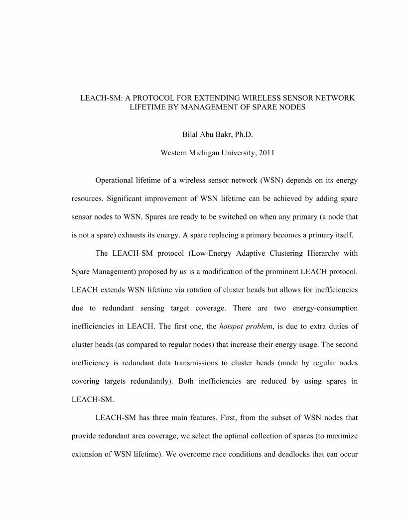
2.4 Power Modes for Wireless Sensor Nodes
There are two power modes for sensor nodes: the active mode and the passive
mode (cf. Figure 2.3.). Cluster heads and regular nodes are in the active mode, whereas
spares are in the passive mode.
13
Figure 2.3. State diagram for power modes of sensor nodes. (“I” indicates a transition occurring during WSN initialization.)
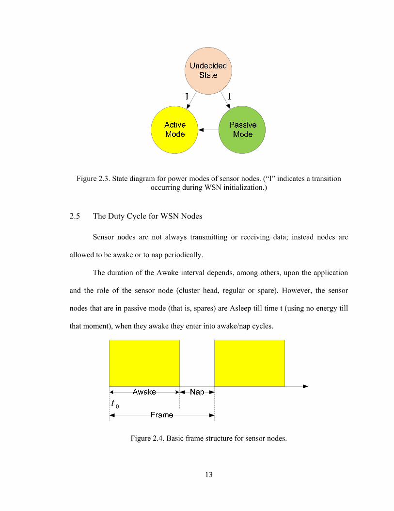
2.5 The Duty Cycle for WSN Nodes
Sensor nodes are not always transmitting or receiving data; instead nodes are
allowed to be awake or to nap periodically.
The duration of the Awake interval depends, among others, upon the application
and the role of the sensor node (cluster head, regular or spare). However, the sensor
nodes that are in passive mode (that is, spares) are Asleep till time t (using no energy till
that moment), when they awake they enter into awake/nap cycles.
0t
Figure 2.4. Basic frame structure for sensor nodes.

14
A frame is the interval during which each regular node sends one message
(consisting of multiple packets) with the sensed data to the cluster head. It includes
Awake and Nap intervals. The frame duration for a node is the sum of its one Awake
interval and one Nap interval [YHE04]. The duty cycle of a node is the ratio of the
duration of its Awake interval to the frame duration (cf. Figure 2.4).
2.6 WSN Failures and Battery Capacity
There are many reasons for WSN failure. We should know the causes of failure
for the sake of prevention. It is rarely practicable to identify a priori all failure causes.
The main reasons of WSN failures are as follows:
1. Battery exhaustion: the failure of WSN due to using out all battery energy for a
certain number of sensor nodes.
2. A defective MAC protocol: Many MAC protocols have been proposed recently to
minimize energy consumption. An inadequate MAC protocol (e.g., one allowing
for too many collisions) can cause a premature WSN failure due to faster energy
consumption.
3. Deterioration: WSNs can fail due to deterioration of its components. Deterioration
is difficult to analyze, because it varies with the type of sensor nodes and the
material used.
4. Environmental conditions: The environmental conditions (e.g., flooding, extreme
temperatures) play a significant role in WSN failures.
There are many other reasons of WSN failures. In this research we consider only
WSN failures due to battery exhaustion in sensor nodes. The restricted battery power of
sensor nodes is the major limiting factor that reduces their operating time. We show that

15
the lifetime of WSNs can be increased by efficient scheduling and proper management of
sensor nodes in WSNs.
The capacity of a battery can be defined by the amount of charge that it can store.
The charge, expressed, e.g., in Coulombs or Ah, can be converted to its equivalent units
in terms of current and time.
(2.5)
where I is current and t is time.
If and are known (and I is the average current used), we can calculate how
long the battery can last as:
B
(2.6)
16
3. RESEARCH GOALS
We propose the LEACH-SM protocol—a modification of LEACH—to realize the
following three most significant goals for extending the lifetime of WSN.
3.1 Goal 1: Optimal Spare Selection
If more than the minimal numbers of sensor nodes than required for above-threshold
coverage are active, then WSN lifetime is shortened. To achieve WSN lifetime extension,
LEACH-SM adds the spare selection phase to LEACH. This phase consists of two
intervals: the sensing range neighbor (SR-neighbor) discovery interval, and the DESST
execution interval (where DESST stands for Decentralized Energy-efficient Spare
Selection Technique).
DESST is a spare management technique that, when executed in parallel by all
regular nodes, decides whether a given node should become a spare or a regular (primary
node i.e., a node that is not a spare). At the moment t0 when the spare selection phase
ends, primary nodes are active (that is, Awake or Napping), while the spares are passive
(that is, Asleep).
DESST maintains the coverage above the target coverage threshold. DESST
consists of: (i) finding the order in which nodes must make the spare/primary decision;
and (ii) actually making this decision. Since sensing ranges for nodes can cross cluster
boundaries, race conditions and deadlocks can occur in Step (ii). We overcome these
challenges.

17
Nodes that became spares provide redundant coverage w.r.t. to the primary nodes.
If not put Asleep by DESST, they would send redundant data to cluster heads.
Importance. DESST achieves the following significant objectives: (i) extending WSN
lifetime; (ii) allowing nodes in all clusters to make primary/spare decisions in parallel;
(iii) reducing transmission of redundant data to cluster heads.
3.2 Goal 2: Management of Spare Nodes after WSN Deployment
To the best of our knowledge, limited attention is paid in the literature to
managing spares. This makes our second research goal for LEACH-SM significant. This
goal is providing a proper spare management in order to decide: (i) how long the spares
should remain Asleep; and (ii) which spare should be used as a replacement for a given
primary node that used up all their energy.
We propose that spares are initially Asleep, and wake up3 to enter the Awake-Nap
cycles at time t4 , 5 (t is estimated by DESST during the spare selection phase). During its
very short Awake intervals, each spare checks with its cluster head if it is needed to
replace a primary. Very short Awake intervals imply very long Nap intervals, which
results in lowered energy consumption by spares that are no longer in the Sleep state.
3 Spares wake up themselves (using a standard built-in time). A cluster head could wake up a sleeping spare only if
special hardware were available.
4 As primary nodes exhaust their energy, the target coverage can decrease from 100% to the threshold value. If spares
are unavailable, the coverage will go down to X% at certain time tX. We set t = tX.
5 The larger is t the more energy is saved by spares. However, if t is too large, some exhausted nodes would have no
spares ready for replacing them.

18
Note that the end of each Awake interval for a spare coincides with the end of the (much
longer) Awake interval for its cluster head.
In contrast to spares, primaries must follow the cycles of Awake and Nap
intervals from the moment t0 of WSN deployment. Their Awake intervals are much
longer, and their Nap intervals are shorter than for spares after time t.
Importance. A proper management of spare nodes saves their energy, making
them available for a longer time for replacing failed primaries. This extends WSN
lifetime.
3.3 Goal 3: Estimating the Lifetime of WSN
A good estimate of WSN lifetime is critical for planning WSN applications. The
power management problem associated with WSNs is conceptually a simple, based on
supply and consumption. In practice, it is complicated by many factors affecting WSN
lifetime. Providing WSN lifetime estimate requires: (i) calculating lifetime for primary
nodes and spares; (ii) calculating duty cycles for all types of nodes; and (iii) estimating
lifetime of node batteries.
Importance. A good estimate of WSN lifetime has a fundamental importance for
planning WSN applications.

19
4. RELATED WORK
In this section we briefly report on the work performed on the presented problem
by other researchers. A number of topology management algorithms and schemes have
been proposed to increase WSN lifetime. This section discusses briefly the main results
of the most relevant work related to lifetime extension and power management for
WSNs.
Figure 4.1. Three main categories of solutions extending WSN lifetime.
The solutions extending WSN lifetime can be divided into three main classes (cf.
Figure 4.1): (i) Data Aggregation solutions, (ii) MAC Protocol solutions, and (iii)
Scheduling of sensor nodes solutions..
The design a MAC protocol deals with energy aware routing, low duty cycle,
energy-efficient communication protocols, etc. Data aggregation solutions deal with
techniques like coding (combines incoming data), adaptive data propagation, etc.
Topology management solutions consider efficient scheduling and management of

20
individual sensor nodes, clustering of nodes, energy level assignment to nodes, and
deployment of redundant nodes, appropriate scheduling techniques, etc.
There is a lot of research being done on solutions in the areas of Data Aggregation
and MAC Protocol, but less research in the area of WSN topology management in terms
of scheduling and management of sensor nodes.
Heinzelman [Hein00] designed and implemented Low-Energy Adaptive
Clustering Hierarchy (LEACH) protocol for WSN. LEACH uses a clustering
architecture. Each cluster elects a cluster head. For balancing energy load in the network,
LEACH rotates the energy-thirsty function of the cluster head among all the nodes in a
cluster. To avoid data transmission collisions, LEACH uses a time division multiple
access (TDMA) protocol. The major characteristics of LEACH include randomized,
adaptive, and self-configured cluster formation; localized control for data transfer; low-
energy media access; and application-specific data processing for data aggregation or
compression.
Zhang et al. [ZLX08] introduced the Efficient Power and Coverage Algorithm
(EPCA) that puts the redundant sensor nodes into the sleep mode while maintaining the
sensing field fully covered. The idea of EPCA is that any sensor node turns itself off if
the so called coverage degree of its neighbors is not affected. Authors introduce two
modes in the scheduling phase: active and passive. Every sensor node in the passive
mode wakes up periodically to receive beacon messages from sensor nodes that are in the
active mode. It is not clear which sensor node will decide first to go to sleep. Moreover,
the periodic wake-up schedule for the sensor nodes those are in the passive mode remains
unspecified.

21
Zhou et al. [ZXWP06] present energy efficient data dissemination (EEDD)
protocol. They consider two-level node activity schedules: coarse and fine. At the coarse
schedule level, only a necessary set of working sensor nodes are kept Awake, and other
sensor nodes are enter the long-term sleep state. All sensor nodes decide their state
through a detection process. In the detection process, a sensor node playing the detecting
node function broadcasts a detecting message to its neighbors to detect the number of
active nodes within its detection range. If a working node in the detection range of the
message sender has energy higher than a pre-specified value Egridhead, it sends back a
response message. If the number of response messages received by the detecting node
exceeds a pre-defined threshold, the detecting node considers itself a redundant and
enters the long-term sleep state; otherwise, the detecting node enters the working mode.
The protocol proposed by Gallais et al. [ACSS06] deploys sensor nodes randomly
over a square area. An active WSN node belongs to one of the k layers, where a layer
provides a full coverage of the sensing area. In other words, the sensing area is covered
redundantly k times k layers.
Suppose that we look at the protocol at the moment that j<k layers have already
been created. But there are still nodes that do not belong to any of these j layers. Let
Node A be one of these nodes that do not belong to any layers yet. Node A listens to
activity messages from its neighbors. For example, the neighbor Node B belonging to
Layer i includes in its activity message the identifier i of the layer to which it belongs. In
this way, node A finds out all layers that cover its location and the degree of coverage
redundancy for its location. Suppose that node A finds out that its location is covered 2
times and the required degree of coverage redundancy must be 3. Node A turns itself ON

22
and sends the activity message to all its neighbors stating that it belongs to layer 3. Any
redundant node that does not belong to Layer 1 or Layer 2 can now decide to join Layer
3. This is the basic idea of the protocol for assuring that sensing area is k-covered.
Lai et al. [LWYW06] propose a genetic algorithm to find an approximate solution
for the NP-complete Disjoint Set Covers (DSC) problem. They consider extending the
WSN lifetime by dividing all sensors into disjoint sensor subsets, or sensor covers, and
each sensor cover needs to satisfy the coverage constraints. Only one sensor cover is
active to provide the functionality and the remaining sensor covers are in the sleeping
mode. Once the active sensor cover runs out of energy and consequently cannot maintain
coverage constraints, another sensor cover will be selected to enter the active mode and
provide the functionality continuously. The more sensor covers we can find, the longer
sensor network lifetime will be prolonged. Finding the optimal number of sensor covers
can be solved via transformation to the DSC problem.
Chamam et al. [ChPi907] address the problem of maximizing the WSN lifetime
under the area coverage constraint. They propose a scheduling mechanism that, for every
time slot during the operating period, calculates an optimal covering subset of sensor
nodes; only those nodes are activated for the given period and the remaining ones are put
to sleep.
Ren et al. [RGM08] propose an initial energy assignment (IEA) strategy, which
increases WSN lifetime by providing different initial energy levels to different sensor
nodes. The nodes that play more energy-consuming functions get more initial energy.
This is in an attempt to assure that all nodes, independent of their function, use up their
available energy at (nearly) the same moment.

23
Dasika et al. [DVCR04] present an algorithm that determines the schedule for
transitioning sets of sensor nodes between active and inactive states that satisfy user-
specified performance constraints. Each sensor node remains in the undecided state until
all of its “weaker” neighbors choose their state (a node is “weaker” when it has less
energy).
Esseghir et al. [EsPe08] optimize the wireless sensor network lifetime under a
reliability constraint. They introduce a function that links reliability to the average
amount of energy consumed by the network when reporting an event to the base station.
Based on this function, they bring out the required number of successive readings to be
performed in order to optimize both network lifetime and reliability.
They also give an altered definition of reliability in order to maximize the
network lifetime by relaxing the reliability restriction. In this case, the reliability is
defined w.r.t. the number of non-reported events.
Mak et al. [MaSe09] they study different WSN protocols based on various WSN
lifetime definitions. They classify WSN protocol and different WNS lifetime definitions.
With the help of simulation they compare performance of WSN protocols.
Hasegawa et al. [HKTM09] propose a routing reconfiguration method based on
an autonomous optimization of the dynamics of mutually connected neural network
which minimizes its own energy function using autonomous and distributed computing.
They also show that the proposed method can optimize routes for maximizing the
lifetime of the sensor network, without any centralized computing nodes.
Xiong et al. [XLY09] prove that the problem of maximizing the lifetime of a
data-gathering sensor network, which is defined as the number of rounds until the first

24
node depletes its energy, is NP-complete. They then formulate it as an integer program to
get a suboptimal result. They further propose a polynomial-time and provably near-
optimal algorithm to reduce the tremendous computation and storage cost of integer
programming. Finally, they evaluate the efficiency of their algorithms by extensive
experiments.

25
5. DETAILED ANALYSIS OF THE INEFFICIENCY PROBLEM IN LEACH
This section discusses in detail inefficiencies in LEACH, which can be eliminated
to extend WSN lifetime. It calculates the duration of the Awake interval, the duty cycles,
and average current drawn by cluster heads and regular nodes in LEACH. Next, it
calculates WSN lifetime for LEACH and its two main variants, named LEACH-C
(LEACH-Centralized) and LEACH-F (Fixed Cluster, Rotating Cluster-Head). Finally, it
calculates residual WSN lifetime for LEACH, LEACH-C, and LEACH-F.
1
Figure 5.1. Rounds, phases, and frames for one cluster (with a cluster head and nc regular nodes) in LEACH.

26
5.1 Timeline of LEACH
The operation of LEACH is divided into rounds as shown in Figure 5.1. Each
round is further subdivided into a (cluster) setup phase and a steady state phase. In each
round, a new cluster configuration is formed,6 and a new cluster head is selected from
among the nodes that have not served as a cluster head in previous rounds. The lifetime
estimate algorithm in LEACH assures with a high probability that LEACH will not run
out of candidate cluster heads that did not serve as a cluster head yet. In other words, for
each round an appropriate node that did not serve as a cluster head yet is found with
a high probability.
The number of rounds in LEACH is determined as N/K, where N is the number of
WSN nodes, and K is the expected number of clusters.
The steady state phase is further subdivided into frames. A frame is the interval
during which each regular node sends one message (consisting of multiple packets) with
the sensed data to the cluster head. Note that the number of frames per round is an
optimization parameter that is used to maximize WSN lifetime in LEACH (also in
LEACH-SM).
As shown in Figure 5.1, the frame duration for a node is the sum of either: (i) one
Awake interval and one Nap interval (for Nodes 1 and 1 in Figure 5.1); or (ii) one
Awake interval and two Nap interval (for Nodes 2, 3, …, 2 in Figure 5.1). Note that
the total time spent napping is the same for cases (i) and (ii).
A round duration depends on the number of frames contained within the round.
The number of frames for a given round in LEACH is determined in a way that
6 In each round, the number of clusters is determined anew. That is, in general, a different number of clusters is formed
in each round.

27
(statistically) ensures that each node’s energy is sufficient to allow the node to be a
cluster head once (during one round) during WSN lifetime and to be a regular node
during the remaining 1 rounds of WSN lifetime.
5.2 The Inefficiency in LEACH
As discussed earlier, the main reason of inefficiencies in LEACH is the inefficient
use of redundant sensor nodes.
S
R / P
Awake
Frame
Nap
Frame
Nap12
3
Regular Nodes
Cluster Head
1
Figure 5.2. Timing of awake and nap intervals for a cluster head and its 1 regular nodes. (Awake periods shown in gray, and Nap periods shown in white.)
In a WSN with N sensor nodes and Ki clusters in Round i, there are N-Ki regular
nodes (summed across all clusters) allowed to transmit data to their cluster heads.
Let nc be the number of nodes in the current cluster. Then, the Awake interval of
the cluster head should be long enough to accommodate arrival of all messages from
1 regular nodes of the cluster. Therefore, the average receiving window size for the

28
cluster head must be at least 1 , where is the average time that a
regular node needs to transmit a message with sensed data to its cluster head (cf. Figure
5.2).
Figure 5.2 shows that each Awake period for cluster heads consists of two major
parts: the receiving and processing interval R/P (for data from regular nodes), and the
transmitting interval Tb (for data sent to the base station). Figure 5.2 also shows that each
Awake period for regular nodes consists of two major parts: the sensing interval S, and
the transmitting interval Tch (for data sent to the cluster head).
To prevent collisions among regular nodes sending data to their cluster heads, the
transmission intervals for the regular nodes are carefully scheduled (as shown in Figure
5.2 by non-overlapping Tch intervals for the regular nodes). The last Tch interval for
a primary ends soon enough to leave at least time Tb of the Awake period available to the
cluster head for data transmission to its base station.
As mentioned earlier, there are two energy-consumption inefficiencies for cluster
heads in LEACH. First, there is the hotspot problem: due to its extra duties, a cluster head
uses more energy than regular sensor nodes. Second, the regular sensor nodes with
overlapping target coverages generate redundant data, which creates unnecessary load on
cluster heads.
LEACH does not propose a complete solution to either of these problems. It
incorporates well-planned rotation of the cluster head role among all nodes in a cluster,
and ensures that (with a high probability) all nodes serve as a cluster head only once
during WSN lifetime; in this way LEACH tries to even out long-term energy usage by all

29
nodes in a cluster. However, LEACH does not compensate for the loss of energy suffered
by a node during its cluster head service.
The well-planned rotation of the cluster head role is the only partial solution for
the first problem given in LEACH. LEACH does not give solutions for the second
problem.
5.3 Notation
Table 5.1 shows notation used in this research. If values of a variable X are the
same in LEACH and LEACH-SM, we use to denote the variable. Otherwise, we use
to denote the variable in LEACH and to denote the variable in LEACH-SM.
Table 5.1. Notation.
Symbol Description
Initial battery charge
Battery energy consumed during all R cluster setup phases in
LEACH/LEACH-SM
The charge consumed by a cluster head during all frames of a single
round
The remaining battery charge for all cluster head and regular node
activities
The remaining battery charge for all regular node activities
l Data packet size without header
∗ Data packet size without header

30
Table 5.1 – Continued
/ Size of data received by a cluster head from a regular node in
LEACH/LEACH-SM
/ Duty cycle of a cluster head in LEACH/LEACH-SM
/ Duty cycle of a regular node in LEACH/LEACH-SM
Number of frames per round in LEACH/LEACH-SM
/ Average current drawn by a cluster head for the Awake interval in
LEACH/LEACH-SM
Average current drawn by a cluster head for receiving messages
from regular nodes in LEACH/LEACH-SM
Average current drawn by a cluster head for storing and aggregation
of the received data in LEACH/LEACH-SM
Average current drawn by a cluster head for sending data in
LEACH/LEACH-SM
Average current drawn by a regular node during the Awake interval
in LEACH/LEACH-SM
Average current drawn by a regular node for sensing and logging the
sensed data in LEACH/LEACH-SM
Average current drawn by a regular node for sending data in
LEACH/LEACH-SM

31
Table 5.1 – Continued
Average current drawn by the spare sensor node duration the Awake
interval LEACH-SM
Average current drawn by nodes during spare selection phase in
EACH-SM
Number of WSN clusters (and cluster heads)
/ / / WSN lifetime for LEACH/LEACH-C/LEACH-F/LEACH-SM
/ /
/
Residual WSN lifetime for LEACH/LEACH-C/LEACH-F/LEACH-
SM
/ Lifetime and residual lifetime for a spare in LEACH-SM
Number of WSN nodes
Number of nodes in a cluster
/ Number of rounds in LEACH/LEACH-SM
Average data transmission rate from a regular node to its cluster
head or from a cluster head to a base station in LEACH/LEACH-SM
Average frame length, that is, the average duration of the Awake
interval + the average duration of the Nap interval in
LEACH/LEACH-SM
Total charge consumed by the node during all setup phase in
LEACH / LEACH-SM

32
Table 5.1 – Continued
/ Total charge consumed by cluster head in LEACH / LEACH-SM
Total charge consumed by regular node in LEACH / LEACH-SM
/ Total charge consumed by each node during its lifetime (and WSN
lifetime) in LEACH / LEACH-SM
/ Duration of a Nap interval of a cluster head in LEACH/LEACH-SM
/ Average duration of the Nap interval of a regular node in
LEACH/LEACH-SM
/
Duration of the setup interval in LEACH/LEACH-SM
Average current drawn by a node during setup phase in
LEACH/LEACH-SM
The ratio of cluster nodes (with the cluster head excluded) that
become spares in LEACH-SM
/ The factor by which data aggregation process reduces data size in
LEACH/LEACH-SM
/ Duration of the Awake interval of a cluster head in LEACH/
LEACH-SM
/
Time taken by a cluster head for receiving and logging (storing)
messages from regular nodes in LEACH/LEACH-SM

33
Table 5.1 – Continued
/ Average time taken by a cluster head for aggregation of data
received from its regular nodes in LEACH/LEACH-SM
/ Time taken by a cluster head for sending data to its base station in
LEACH/LEACH-SM
Duration of the Awake interval of a regular node in
LEACH/LEACH-SM
Time taken by a regular node in sensing and logging sensed data in
LEACH/LEACH-SM
Time taken by a regular node for sending data to its cluster head in
LEACH/LEACH-SM
Duration of the Awake interval for a spare node in LEACH-SM
Duration of the spare selection interval in LEACH-SM
5.4 Calculating Duration of Awake Interval for LEACH
In this section, we calculate the duration of Awake intervals for cluster head and
regular nodes in the LEACH protocol. Note that, Awake interval is different for each
kind of sensor nodes. It depends upon many factors such as data processing, logging rate
and data transmission/receiving rate of sensor node and roll of the sensor node. The
Awake interval should be long enough to accommodate a single and data bit
transmit/receive.

34
Figure 5.3. Different periods within a frame for a cluster head and regular nodes in LEACH. The arrows from Regular Nodes to Cluster Head denote transmissions of sensed
data. T is frame duration.
5.4.1 DurationofAwakeIntervalforRegularSensorNodes
Regular sensor nodes collect a certain number of samples (raw data) at a chosen
sampling rate from their sensing hardware (onboard sensors) and log (store) the samples
into its persistent storage (EEPROM) [Tin02]. At regular time intervals, regular nodes
retrieve data from their storage, and transmit them to their cluster heads.
The length of the Awake interval for a regular node (shown in gray in Figure 5.3)
is the sum of the durations for the sensing/logging period and the sending
period . The former depends on the required number of samples and the sampling
rate,7 and the latter depends on the data transmission rate.
7 The sampling rate is determined by the application using the WSN.

35
Assuming that the analog sensors of a regular node gather data at up to 1,280
samples per second, and the ADC unit of the node (cf. Figure 2.1) produces 10 bits per
sample, the regular node produces 12,800 bits of sensed data per second.
Let the length of a message sent by a regular node to its cluster head be bits.
Then, time taken by a regular node for sensing (and logging) bits of data is:
/ 12,800 (5.1)
Let the transmission rate from the regular sensor node to the cluster head be r
bits/sec, and let be the total length of the packet headers for the packets constituting the
messages (with l bits of data). Then, time taken by a regular node for transmitting
∗ bits of sensed and header data is:
∗, ∗/ (5.2)
The length of the Awake interval for a regular node is:
, ∗, ∗, (5.3)
5.4.2 DurationofAwakeIntervalforClusterHead
The duration of the Awake interval for cluster heads (shown in gray in Figure 5.3)
depends upon: (i) the number of primary nodes within the cluster, and (ii) the data
transmission rate for the regular nodes.
Let nc be the number of primaries in the current cluster. The receiving window for
the cluster head is the time taken by the cluster head for receiving and logging messages
from all nc – 1 regular nodes. The required (minimum) average length of the receiving
window for a cluster head is:
∗, ,

36
= 1 ∗, (5.4)
Regular nodes with overlapping target coverage generate redundant data. A
cluster head is responsible for receiving such redundant data, and aggregating them. Data
aggregation techniques eliminate data redundancies, and reduce the number of data
packets that the cluster heads sends to its base station [Hein00].
Time taken by a cluster head for data aggregation depends upon the number and
size of messages received from regular nodes. Let be the average time taken by the
cluster head to aggregate one bit of data ([sec/bit]). The cluster head receives
1 ∗bits of data (recall that l* is the message length). Hence, time used by a
cluster head for data aggregation is:
∗, ,
1 ∗ (5.5)
Regular nodes with overlapping target coverages generate redundant data. After
receiving all data from regular nodes, the cluster head aggregates received data, reducing
data size by a factor of % ; 0 100.
Since the total size of sensed data received by a cluster head is 1
∗ bits], then the aggregated data size is:
, ∗ , 1 ∗ (5.6)
The average time taken by the cluster head to forward the aggregated data to
its base station at the transmission rate r [bits/sec] is:
, ∗, , , ∗, /
1 ∗/ (5.7)

37
From Equations (5.5), (5.6) and (5.7), the total average time during which the
cluster head remains Awake is:
, ∗, , ,
∗, , ∗, , , ∗ , , (5.8)
Note that depends, among others, upon the number of nodes nc in the given
cluster.
5.4.3 DurationofNapIntervalforClusterHead
The Nap interval for a cluster head (cf. Figure 5.3) is:
, ∗, , , , , ∗, , , (5.9)
where T is the frame length. If a cluster head remains awake continuously, then
and 0;otherwise, 0.
Since from Equation (5.8) is much larger than from Equation (5.3), a
cluster head must stay awake for a much longer period than a regular node. This explains
why it consumes much more energy than a regular node.
5.5 Calculating Duty Cycle for LEACH
Primary nodes are not always Awake (transmitting or receiving data); they may
Nap to save energy whenever they need not be Awake. (So primaries follow cycles of
Awake and Nap intervals, as shown in Figure 5.1.)
The duty cycle for a node is defined as the ratio of the length of its Awake interval
to the frame duration.

38
The length of the Awake interval for a cluster head depends upon the number of
regular nodes within the cluster. This puts a lower limit on the frame length. We cannot
set it shorter than the duration of the Awake interval of the busiest cluster head;
otherwise, this cluster head would be unable to receive data from all regular nodes within
its cluster.
Once we set the frame length (considering the busiest cluster head), the duty
cycles for all WSN nodes will be affected. In other words, the duty cycle for each WSN
node depends upon the duration of the Awake interval of the busiest cluster head.
In calculating duty cycles for all nodes, we need to look at two cases: (i) when the
duration of the Nap interval for the cluster head is zero, and (ii) when the duration of the
Nap interval for the cluster head is not zero.
5.5.1 Case1:DurationofNapIntervalforClusterHeadisZero
5.5.1.1 Calculating the Duty Cycle for Cluster Head
When the duration of the Nap interval is zero, a cluster head will remain in
the Awake mode continuously, that is, . In this case, the duty cycle for a cluster
head is:
, ∗, , , , , ∗, , , / T T/T 100% (5.10)
5.5.1.2 Calculating the Duty Cycle for Regular Nodes
The duty cycle for a regular node is:
, ∗, , , ∗, / 100% (5.11)

39
5.5.2 Case2:DurationofNapIntervalforClusterHeadisNotZero
5.5.2.1 Calculating the Duty Cycle for Cluster Head
If 0, the duty cycle for a cluster head is:
, ∗, , , ,
, ∗, , , /T 100 , ∗, , , , 100 % (5.12)
5.5.2.2 Calculating the Duty Cycle of Regular Nodes
In this case the duty cycle of regular nodes is:
, ∗, , , ∗, / 100% (5.13)
5.6 Energy Consumption Model for LEACH
In this section, we show the energy consumption model for LEACH. We focus
here on a single WSN sensor node, even though the final goal is calculating WSN
lifetime. As was mentioned, we assume that energy, needed for sensing, logging data, and
sending/receiving of data [Dress07], is provided by node batteries.
We are using the sensor node model shown in Figure 2.1 (it is more detailed than
the model given in Ref. [Hein00]). The sensor node components primarily contributing to
the overall energy consumption are: the on board sensors, the analog-to-digital converter
unit (ADC), the micro controller, and the communication module (including the sending
and receiving modules. Energy consumed in the process of sampling, processing and
logging data by a sensor node is comparable to the energy consumed by the sender and

40
receiver circuits of the sensor node. To run all components, the Microcontroller needs be
Awake all the time.
Energy consumption by a node includes: (i) energy consumption during sensing
and logging (incl. energy consumed by the onboard sensors), (ii) energy consumption
during sending and receiving data. (In our analysis we ignore small amounts of energy
needed by regular nodes to receive rare and short messages from their cluster heads, and
by cluster heads to send these messages to regular nodes.)
Knowing time spent by each node in each state, as well as the current drawn by
the node circuitry in each state [Dress07], we can calculate the average energy consumed
by each node.
5.6.1 AverageCurrentDrawnbyRegularNodes
Let and be the average current used by a regular node during
sensing and logging, and the average current used by the node during sending data to its
cluster head, respectively. Then, the average current consumed by a regular node during
its Awake interval is (all parameter lists omitted):
(5.14)
5.6.2 AverageCurrentDrawnbyClusterHeads
Let be the average current drawn by a cluster head during receiving
messages from regular nodes, —the average current drawn by it during aggregation of

41
received data, and —the average current drawn by it during sending data to the base
station. Then, the average current drawn by a cluster head during its Awake interval is:
(5.15)
5.7 Special-case Calculation of WSN Lifetime for LEACH
As is often the case, obtaining a closed formula describing a complex
phenomenon is impossible (or, at least, beyond time or capability limitations of the
analyzers). Instead, obtaining a closed formula is limited to a special case of the
phenomenon, in which simplifying assumptions facilitate obtaining a closed formula.
The results obtained for a special (simplified) case are still very useful. They can
be used to validate results of extensive simulations run for the original general case,
“described” by the simulation in its full (or at least much more complete) complexity.
Unable to provide a closed formula for determining WSN lifetime in its full
complexity, we make simplifying assumptions in this chapter.
Let N be the number of all WSN nodes, and K be the number of clusters in Round
1. We assume that: (i) remainder(N/K) = 0, i.e., N is evenly divisible by K; (ii) the
number of clusters in each round is K, (iii) all clusters are of size R = N/K (recall that R is
the number of rounds); as a consequence, duration of all frames for all rounds is identical
(because during each frame the same number of regular nodes need to send sensed data to
their cluster heads); (iv) in each round LEACH finds a good cluster node; that is, in each
round LEACH finds an appropriate node that did not serve as a cluster head in previous
rounds; and (v) the number of frames F per round is constant (recall that F is the

42
optimization parameter that allows to maximize WSN lifetime); and (vi) no current is
drawn by nodes during their Nap intervals.
As a consequence of Assumption (iii), we will have R rounds during WSN
lifetime. The simplest way of realizing Assumption (iv) is by using the cluster
configuration created in Round 1 in all remaining rounds as well. Assumptions (iii) and
(iv) assure that each node plays the cluster head role only once.
Before providing a closed formula for determining WSN lifetime, we first
calculate the number F of frames per round (an optimization parameter for WSN lifetime
in LEACH). F needs be calculated before we can calculate WSN lifetime. Finding F is
the most complex part of finding WSN lifetime L.
Theorem 1: Let be the initial battery charge; —the average current
drawn by the cluster head (more precisely, by a node playing the role of a cluster head)
during its Awake interval; —the average current drawn by a regular node (more
precisely, a node playing the role of a regular node) during its Awake interval; —
the average current drawn by a node during the cluster setup phase; —the number of
rounds; and —the durations of the Awake intervals for a regular node and a
cluster head, respectively; and —the duration of the setup phase. Then the number
of frames F per round in LEACH is:
36001
(5.16)
Proof: With N and K being the number of all WSN nodes and the number of
clusters in each round, the total number of rounds is R = N/K (where, as assumed,

43
reminder(N/K) = 0). By our assumptions, R is also equal to the number of nodes in each
cluster.
According to LEACH, each primary will be a cluster head exactly once in its
lifetime. This means that it will be a regular node for 1 rounds.
The following consideration will be easier to follow when looking at Figure 5.1.
During the setup phase, the node consumes the charge equal to .
Since the phase is repeated in each round, the total charge consumed by the node during
all setup phase is:
/3600 [Ah] (5.17)
Since a node plays the cluster head role in exactly F frames of one round during
WSN lifetime, the charge it consumes during its entire cluster head service during WSN
lifetime is:
/3600 (5.18)
Since a node plays the regular node role in exactly F frames of R-1 rounds during
WSN lifetime, the charge it consumes during its entire regular node service during WSN
lifetime is:
1 /3600 (5.19)
Hence, the total charge consumed by each node during its lifetime (and WSN
lifetime) is:
1 /
3600

44
If the node uses all energy available to it from its battery (its full initial charge
Bcap), then . Hence:
1
/3600
36001
(5.20)
Q.E.D.
Theorem 2: Let dCH and dReg be duty cycles for cluster heads and regular nodes,
respectively; F—the number of frames per round; R—the number of rounds during the
entire WSN lifetime; —the duration of the setup phase; T—the duration of each
frame; and the remaining symbols—as defined in Theorem 1. Then, WSN lifetime L for
LEACH is:
3600 (5.21)
Proof: A setup overhead is paid only once, at the beginning of the each round. If
is the initial battery charge and is the battery energy consumed during all R
cluster setup phases, then:
(5.22)
The energy remaining for all node activities other than cluster setup (i.e. for
cluster head and regular node activities) is:
(5.23)

45
In its lifetime, each primary node serves as a cluster head only once during a
single round. The charge consumed by a cluster head during all frames of that single
round is: .
The remaining battery charge for all regular node activities (during all frames in
R-1 rounds) is:
= [ ]
This charge is fully consumed by the node during all its regular-node activities (in
all frames of R-1 rounds). Therefore, the charge consumed by a node during its regular-
node activities is: .
The WSN lifetime L in LEACH is approximately equal to the lifetime of any
primary node (since LEACH tries to assure that all nodes die at the same time). The latter
consist of the node’s lifetime as a cluster head plus the node’s lifetime as a
regular node. Hence, WSN lifetime L is:
Thus:
(5.24)
Q.E.D.

46
5.8 Calculating WSN Lifetime for LEACH-C and LEACH-F
Two main variants of LEACH are LEACH-C (LEACH-Centralized) and
LEACH-F (Fixed Cluster, Rotating Cluster-Head).
As stated above, LEACH incorporates well-planned rotation of the cluster head
role, as well as adaptive self-configuration cluster formation in each round (cf. Figure
5.1). LEACH-C differs from LEACH only by using a centralized control algorithm to
form better clusters. Therefore, we can use Theorem 2 to calculate WSN lifetime for
LEACH-C:
In contrast to LEACH, LEACH-F forms clusters only once at the beginning of
Round 1 (then, for each round, new cluster heads are selected within the fixed clusters).
Therefore, a setup overhead is paid only once. Thus, we can get WSN lifetime for
LEACH-F by replacing R in Theorem 2 with the value 1. Then, WSN lifetime for
LEACH-F is:
(5.25)
5.9 Residual WSN Lifetime for LEACH and its Variants
The residual WSN lifetime at time t is defined as the remaining life expectancy for
the WSN, given that WSN is alive at time t. A residual lifetime assessment helps in
identification of sensor nodes with low energy resources.
The residual WSN lifetime for LEACH and LEACH-C at any time is:

47
0 (5.26)
Similarly, the residual WSN lifetime for LEACH-F at any time is:
0 (5.27)

48
6. LEACH-SM – THE PROPOSED SOLUTION TO THE LEACH INEFFICIENCY PROBLEM
6.1 Cluster Setup Phase of LEACH-SM
LEACH-SM starts with the cluster setup phase (cf. Figure 6.1). During this setup
phase sensor nodes organize themselves into local clusters, with one node in each cluster
selected as the cluster head.
1
Figure 6.1. Rounds, phases, and frames for LEACH-SM, including the added spare selection phase. Note that spare selection is done only once in WSN lifetime.
Each regular node (a node that is not a cluster head) knows its cluster head and
the received signal strength RSSCH of the advertisement messages from the cluster head.

49
6.2 Spare Selection Phase of LEACH-SM
The spare selection phase (cf. Figure 6.1) consists of two intervals: the sensing
range neighbor discovery interval, and the interval during which DESST (Decentralized
Energy-efficient Spare Selection Technique) is run (to increase wireless sensor network
lifetime).
6.2.1 Interval1:SensingRangeNeighborDiscovery
During the sensing range neighbor (SR-neighbor) discovery interval each regular
sensor node s discovers its sensing-range neighbors (SR-neighbors) in the following way.
First, node s broadcasts a hello message, which is received by all nodes within its
sensing range (we assume realistically that the transmission range exceeds the sensing
range of a node). The hello message contains of the sender node s and of the
static targets ( ) covered by s.
The recipient r of the hello message replies with the hello-reply message
sent back to s. The hello-reply message contains ID of its sender r, r’s cluster ID,
r’s RSSCH, and IDs of the static targets ( ) covered by r.
Upon receipt of the hello-reply message from r, node s stores information
brought by the message (i.e., ID, cluster ID, , ) in s’s SRN table. SRN table is
a local database of information about SR-neighbors of the node.
Using target information received in the hello-reply message from r,
node s can quickly find out if r received the s’s hello message but does not cover any
targets covered by s. In this way s identifies all and only nodes that have sensing ranges
overlapping with its own sensing range, that is, nodes that are s’s SR-neighbors.

50
11
22
Figure 6.2. Illustration for SR-neighbor discovery.
Let us consider an example shown in Figure 6.2. The sensor nodes and are in
the cluster with cluster head , and nodes and are in the cluster with cluster head
. The sensor nodes , , and have received signal strengths
, , , , respectively, where . The sensor nodes
, areincluster and the nodes , areincluster . (The cluster heads for
clusters and are not shown in the Figure 6.2.) Target is covered by and . All
four nodes are SR-neighbors for each other.
After the hello/hello-reply message exchange is completed by all pairs of
the four nodes, their SRN tables look as shown in Figure 6.3 (to avoid clutter,
entries are not shown).

51
Figure 6.3. The SNR tables for four nodes after the hello—hello-reply message exchanges by them.
Recall that: as the set of all SR-neighbors of . That is:
∶ ∈ (6.1)
Let be a node from cluster . Then, the set of all SR-neighbors of from ,
denoted by , , is:
SRN(sm , Cj) = { sp: sp ϵ SRN(sm) ∧ sp ϵ Cj } (6.2)
The set of all SR-neighbors of can be expressed as:
,∈ , , ,… ,
(6.3)
Recall that is the set of all SR-neighbors of excluding itself,
that is:
(6.4)
For each ∈ , there exists )—the set of targets covered by node
. E.g., if targets , and are covered by sensor node , then TS( , , .

52
6.2.2 Interval2:RunningtheDecentralizedEnergy‐efficientSpareSelectionTechnique(DESST)
DESST is a part of the spare management that allows (in parallel across all
clusters) each regular sensor node to select being a primary node or a spare as shown in
Figure 6.4. The former enter the active power mode (they will be awake or napping at the
moment when the spare selection phase ends—cf. Figure 6.1). The latter enter the passive
power mode (they will be Asleep at the moment when the spare selection phase ends). At
the same time, the above-threshold target coverage is assured.
All Deployed Nodes
Primary Nodes
Spare Nodes
DESST
Figure 6.4. DESST puts each WSN node into either passive or active power mode. The former become regular (primary) sensor nodes, and the latter—spare sensor nodes.
Sensing targets can cross cluster boundaries (clusters “limit” transmission of
sensing data to the appropriate cluster heads). Due to this fact, we are facing potential
race conditions and deadlocks

53
A race condition occurs in DESST when multiple sensor nodes (from the same or
different clusters) attempts to decide in parallel whether they should become primaries or
spares.
Consider a situation when target A is covered only by two nodes and , that
belong to clusters and , respectively (as shown in Figure 6.2. Suppose that
decides that it is redundant (since it knows that target A is covered by its SR-neighbor
), and decides to become a spare. In parallel, decides that it is redundant (since it
knows that target A is covered by its SR-neighbor ), and decides to become a spare. As
a result of this race condition, target A will not be covered at all.
A deadlock in DESST occurs when two or more sensor nodes are waiting for each
other before making their primary/spare decision. As a simple deadlock example consider
two sensor nodes , from the same or different clusters. It is possible that waits for
the decision of to make its primary/spare decision, and at the same time waits
for .

54
Algorithm 1: Finding the order in which the nodes from make their
primary/spare decisions
1: for each node do
2: sort elements in the increasing order
3: of their signal
4: if there are groups of nodes tied w.r.t. their
5: RSSCH value
6: then sort each such group on the value of
7:
8: // is now sorted in the order in which
9: // and its SR-neighbors make primary/spare
10: // decision.
11:
12: node finds its position in this ordering
13: // This means that node has to wait with its
14: // decision after 1 other nodes from
15: // make their decision.
Figure 6.5. Pseudocode of Algorithm 1 in DESST.
DESST allows all regular sensor nodes to make their primary/spare decisions in
parallel across all cluster boundaries. It consists of two parts—finding the order of nodes
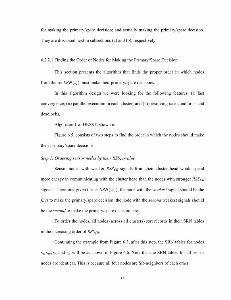
55
for making the primary/spare decision; and actually making the primary/spare decision.
They are discussed next in subsections (a) and (b), respectively.
6.2.2.1 Finding the Order of Nodes for Making the Primary/Spare Decision
This section presents the algorithm that finds the proper order in which nodes
from the set must make their primary/spare decisions.
In this algorithm design we were looking for the following features: (i) fast
convergence; (ii) parallel execution in each cluster; and (iii) resolving race conditions and
deadlocks.
Algorithm 1 of DESST, shown in
Figure 6.5, consists of two steps to find the order in which the nodes should make
their primary/spare decisions.
Step 1: Ordering sensor nodes by their RSSCH value
Sensor nodes with weaker RSSCH signals from their cluster head would spend
more energy in communicating with the cluster head than the nodes with stronger RSSCH
signals. Therefore, given the set , the node with the weakest signal should be the
first to make the primary/spare decision, the node with the second weakest signals should
be the second to make the primary/spare decision, etc.
To order the nodes, all nodes (across all clusters) sort records in their SRN tables
in the increasing order of RSSCH.
Continuing the example from Figure 6.3, after this step, the SRN tables for nodes
, , and will be as shown in Figure 6.6. Note that the SRN tables for all sensor
nodes are identical. This is because all four nodes are SR-neighbors of each other.
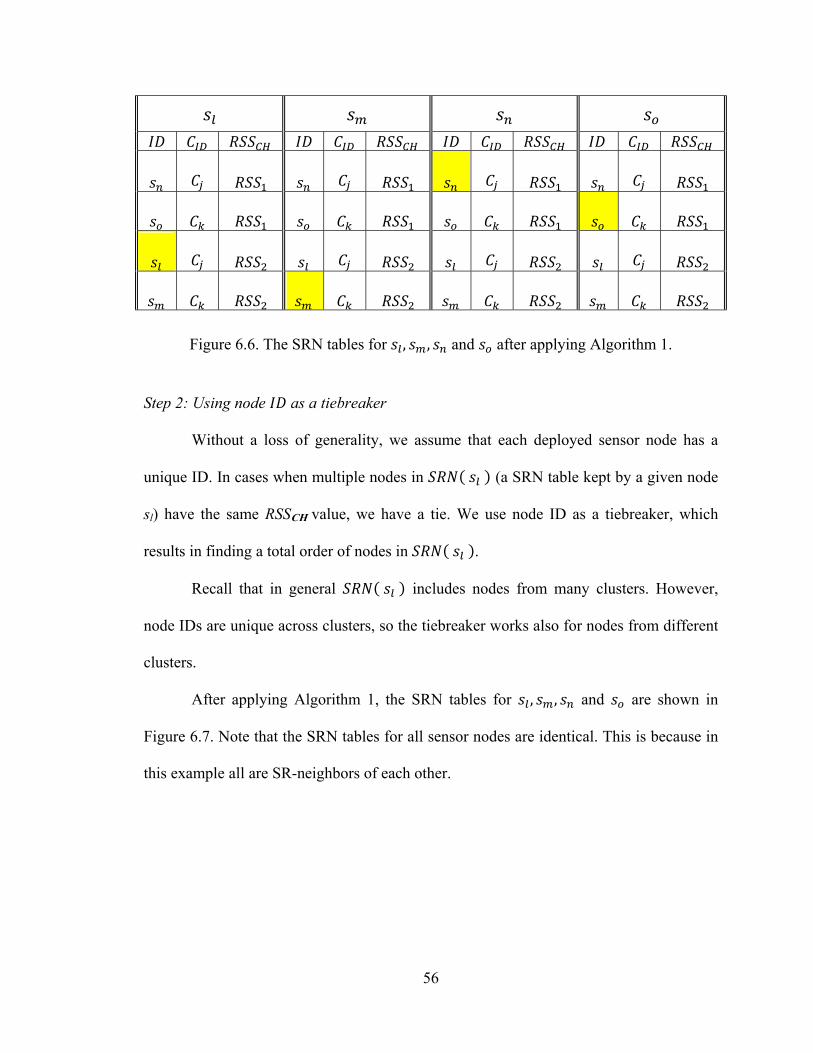
56
Figure 6.6. The SRN tables for , , and after applying Algorithm 1.
Step 2: Using node as a tiebreaker
Without a loss of generality, we assume that each deployed sensor node has a
unique ID. In cases when multiple nodes in (a SRN table kept by a given node
sl) have the same RSSCH value, we have a tie. We use node ID as a tiebreaker, which
results in finding a total order of nodes in .
Recall that in general includes nodes from many clusters. However,
node IDs are unique across clusters, so the tiebreaker works also for nodes from different
clusters.
After applying Algorithm 1, the SRN tables for , , and are shown in
Figure 6.7. Note that the SRN tables for all sensor nodes are identical. This is because in
this example all are SR-neighbors of each other.

57
Figure 6.7. The order in which nodes , , and must make the spare/primary decision.
Let us examine the SRN table of one node in detail. In Figure 6.7, both and
have the same . In this case we use node as a tiebreaker. Since precedes in the
lexicographical order, wins the tiebreaker and decides its mode sooner. Once does
so, can take its turn.
In next section, after finding the candidate position for the deployed sensor nodes,
we show the algorithm for efficient scheduling and management of deployed sensor
nodes. Our algorithm puts each wireless sensor network node into either passive or active
power mode. The former become primary sensor nodes, and the later – spare sensor
nodes. This algorithm also envisages how each sensor node decides its power state in
parallel in each cluster.
In Figure 6.2, nodes and fromcluster and nodes and from cluster
have the received signal strengths RSS2, RSS1, RSS2, and RSS1,resp., where RSS1 >

58
RSS2 (the cluster heads for and are not shown in Figure 6.2 to avoid clutter).
Suppose that target is covered only by and . Also, assume that all four nodes are
SR-neighbors for each other. The nodes with the weakest received signal strengths are
and . Since the ID l precedes the ID m lexicographically, node will be the first to
make the primary/spare decision, and node will be the second to make the
primary/spare decision. The tiebreaker among and is resolved similarly.
Algorithm 2: Primary/spare Decision
1: for each node do
2: find
3:
4: if ⋃ , , ,
5: // if others cover all targets covered by
5: then
6: becomes a spare (passive)
7: else
8: becomes a primary (active)
Figure 6.8. Pseudocode of Algorithm 2 in DESST.
6.2.2.2 Primary/Spare Decision
Target coverage is one of the most fundamental issues in WSN. Maintaining the
required target coverage while reducing the number of sensor nodes is a challenge. A

59
sensor node may decide to become a spare only if the targets covered by it are all
collectively covered by its SR-neighbors. Otherwise, some targets become uncovered,
resulting in WSN coverage holes. The identification of the coverage holes is not simple
and requires extensive investigation
Once the nodes know the order in which they may make their primary/spare
decisions, Algorithm 2 of DESST (Figure 6.8) allows them to make proper primary/spare
decisions.
Node s decides to become a spare (passive) only if all targets covered by s are
redundantly covered by its SR-neighbors (otherwise, some targets would become
uncovered).
Let us illustrate the algorithm. The sensor node is the first to make its
primary/spare decision (cf. Figure 6.6). First, is trying to find out whether
are covering the targets that are covered by or not.
In Figure 6.2, targets covered by , , and are:
∅
∅.
Note that , , . Then we get:
⋃ , , , (6.5)

60
The union gives the set of all targets covered by , so knows what
targets are covered by . Now, takes the intersection of the union with the set
of targets that it covers:
⋃ , , , ⋂ (6.6)
This intersection tells whether all its targets are covered by its neighbors from
. There are two cases here:
Case 1: All targets of are covered by
⋃ , , , ⋂ (6.7)
Figure 6.9. The node becomes a spare and switched into passive mode, estimated by DESST during the spare selection phase.

61
In this case, should become a spare as shown in Figure 6.9. Before becoming
a spare (passive) and going Asleep, transmits its decision to all members of the
neighbor set . After receiving the decision message from , all its SR-
neighbors from update their SRN tables and mark as a spare. Next they
delete entry for from their SRN tables (because no longer covers any targets).
Note that the spares are awakened when the probability that any primary node
exhausted its energy reaches a predefined value.
Case 2: Some targets of are not covered by
Since neighbors of from are unable to cover all targets of , must
become a primary node (active) as shown in Figure 6.10. As before, broadcasts
a message to these neighbors to inform them about making of their primary/spare
decision. Now, the next sensor node can start making its primary/spare decision.

62
Figure 6.10. The node becomes a primary and switched into active mode, estimated by DESST during the spare selection phase.
WSN is vulnerable to various kinds of network problems. For example the
hello message could be lost due to collisions, or a malicious sensor node could flood
WSN with hello messages to break the security of a wireless sensor node (a hello
flood attack on a node). We assume the presence of an appropriate mechanism to prevent
such attacks on WSNs.

63
Targets
J
DA
H
E
G
C
F
B
I
M
K
L
1-80dB 2
-80dB
3-75dB
4-70dB
5-75dB
6-75dB
7-75dB
8-70dB
9-65dB
10-70dB
11-70dB 12
-70dB
13-65dB
14-60dB
15-65dB
16-65dB
17-65dB
18-60dB 19
-0dB
20-60dB
21-70dB
22-70dB 23
-65dB24
-60dB25
-65dB
26-0dB
Received Signal Strength
Figure 6.11. Illustration for Example 1 of SR-neighbor discovery.
6.2.2.3 Example 1: SR-neighbor Discovery (Output of Algorithm 1)
Let us consider 26 sensor nodes randomly deployed in an irregular shaped
geographical region with high density. Due to high deployment density there is very
high probability that each static target will be covered by more than one sensor nodes.
During the setup phase clusters are created and each regular sensor node knows
its cluster head and the distance from it based on the received signal strength .

64
Assume that— as shown in Figure 6.11—sensor nodes and are cluster
heads; sensor nodes , , , and belong to cluster , the remaining nodes
belong to the cluster head ; the and triangles labeled A – M represents targets.
Figure 6.12. Illustration of sending and receiving of a hello message.
Suppose that sensor nodes broadcast the hello messages within its sensing
range. The sensor nodes , , and receive this broadcast hello message coming
from node (cf. Figure 6.12).

65
‐80 , ,
‐80 , , , ,
‐75 , , , ,
‐75 , , , , ,
‐70 , , ,
Figure 6.13. SRN table for node 2 (below target A).

66
After receiving the hello-reply messages from sensor nodes , , and
, node stores the received information in its local SRN table, as shown in Figure
6.13.
In this way, sensor node discovered that sensor nodes , , and are its
SR-neighbors.
After applying the algorithm (cf. Figure 6.5), the SRN tables for all nodes are as
shown in Figure 6.14.
11 6 70 08 9 70 09 9 65 14 9 60 14 9 60
06 6 75 03 9 75 04 9 70 09 9 65 09 9 65
07 9 75 06 6 75 08 9 70 04 9 70 15 9 65
01 6 80 07 9 75 10 9 70 08 9 70 04 9 70
02 9 80 01 6 80 03 9 75 10 9 70 08 9 70
02 9 80 05 9 75 03 9 75 10 9 70
07 9 75 05 9 75 03 9 75
02 9 80 05 9 75

67
16 6 65 13 9 65 14 9 60 19 9 14 9 60
11 6 70 16 6 65 18 9 60 14 9 60 20 9 60
12 9 70 08 9 70 09 9 65 20 9 60 09 9 65
06 6 75 11 6 70 13 9 65 09 9 65 15 9 65
07 9 75 12 9 70 04 9 70 13 9 65 04 9 70
01 6 80 03 9 75 08 9 70 15 9 65 08 9 70
02 9 80 06 6 75 10 9 70 04 9 70 10 9 70
07 9 75 12 9 70 08 9 70 03 9 75
01 6 80 03 9 75 10 9 70 05 9 75
02 9 80 05 9 75 03 9 75
07 9 75 05 9 75

68
13 9 65 18 9 60 14 9 60 14 9 60 14 9 60
16 6 65 13 9 65 18 9 60 18 9 60 20 9 60
17 9 65 16 6 65 24 9 60 20 9 60 09 9 65
11 6 70 17 9 65 09 9 65 24 9 60 15 9 65
12 9 70 08 9 70 13 9 65 09 9 65 25 9 65
21 6 70 11 6 70 16 6 65 13 9 65 10 9 70
06 6 75 12 9 70 17 9 65 15 9 65 05 9 75
07 9 75 21 6 70 23 9 65 25 9 65
01 6 80 06 6 75 08 9 70 04 9 70
07 9 75 11 6 70 08 9 70
12 9 70 10 9 70
21 6 70 05 9 75
22 9 70
07 9 75

69
18 9 60 18 9 60 14 9 60 14 9 60 18 9 60
13 9 65 13 9 65 18 9 60 18 9 60 13 9 65
16 6 65 16 6 65 20 9 60 20 9 60 16 6 65
17 9 65 17 9 65 24 9 60 24 9 60 17 9 65
23 9 65 23 9 65 13 9 65 09 9 65 23 9 65
11 6 70 11 6 70 16 6 65 15 9 65 11 6 70
12 9 70 12 9 70 17 9 65 25 9 65 12 9 70
21 6 70 21 6 70 23 9 65 10 9 70 21 6 70
22 9 70 22 9 70 25 9 65 22 9 70
06 6 75 08 9 70
12 9 70
21 6 70
22 9 70

70
18 9 60 18 9 60 14 9 60 14 9 60
16 6 65 24 9 60 18 9 60 18 9 60
17 9 65 13 9 65 20 9 60 20 9 60
23 9 65 16 6 65 24 9 60 24 9 60
12 9 70 17 9 65 13 9 65 15 9 65
21 6 70 23 9 65 15 9 65 23 9 65
22 9 70 25 9 65 23 9 65 25 9 65
21 6 70 25 9 65 22 9 70
22 9 70
Figure 6.14. Sorted SRN tables for all nodes.
Let us examine the SRN table of one node in detail. The SRN table of is shown
in Figure 6.15. SRN table shows that cannot decide its power state first. It has to wait
for node to decide its power state. On the other hand, the SNR table of shows that it
can decide its power state first without any deadlock and race conditions (cf. Figure
6.16). Once all deployed sensor nodes determine their decision order, then they can
decide their power states in parallel (making them either active or passive) in each
cluster.
After finding decision order for active/passive decision, the process for
determining the state of wireless sensor nodes starts. The sensor nodes that switched to

71
active power mode are active sensor nodes (they will become regular nodes and cluster
heads), and the rest are passive sensor nodes (they will become spares).
02
06
07
01
11
Figure 6.15. The order in which node makes the spare/primary decision.

72
02
08
03
06
07
01
Figure 6.16. The order in which node makes the spare/primary decision.
6.2.2.4 Example 2: Nodes Making the Spare/Primary Decision (Output of Algorithm 2)
To understand how sensor nodes decide their power state, especially those who at
the boundary of the cluster, let us consider the sorted SRN table of all the deployed
sensor nodes. According to the algorithm each sensor node sorts its SRN table. The
sorting process is primarily based on the received signal strength . The overall
picture after sorting SRN tables according to our designed algorithm is shown in Figure
6.14.
Determining the power state of sensor nodes is divided into rounds. Each round
represents a single clock tick, that is, on each clock tick sensor nodes decide their power
state in parallel.
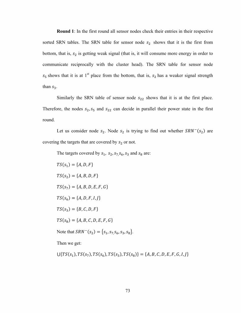
73
Round 1: In the first round all sensor nodes check their entries in their respective
sorted SRN tables. The SRN table for sensor node shows that it is the first from
bottom, that is, is getting weak signal (that is, it will consume more energy in order to
communicate reciprocally with the cluster head). The SRN table for sensor node
shows that it is at 1st place from the bottom, that is, has a weaker signal strength
than .
Similarly the SRN table of sensor node shows that it is at the first place.
Therefore, the nodes , and can decide in parallel their power state in the first
round.
Let us consider node . Node is trying to find out whether are
covering the targets that are covered by or not.
The targets covered by , , , , and are:
, ,
, , ,
, , , , ,
, , , ,
, , ,
, , , , , ,
Note that , , , , .
Then we get:
⋃ , , , , , , , , , , , ,

74
The union gives the set of all targets covered by , so knows what
targets are covered by . Now, takes the intersection of the union with the set
of targets that it covers:
⋃ , , , , ⋂ , , ,
Thus, should become a spare as shown in Figure 6.17. Before becoming a
spare, transmits its decision to all members of the SR-neighbor set . After
receiving the decision message from , all its SR-neighbors from update their
SRN tables and mark as a spare. Next they delete the entry for from their SRN
tables (because is not covering any target covered by them).
08
03
06
07
01
02
Figure 6.17. The node becomes a spare (switches into passive mode) as decided by DESST during the spare selection phase.

75
14
10
04
15
08
03
09
05
Figure 6.18. The node becomes a spare as decided by DESST.
Next we consider node to find out whether are covering the targets
that are covered by or not. The are , , , , , , , and
The targets covered by , , , , , , , and are:
, , , ,
, , , , , ,
, , , ,

76
16
17
23
18
12
21
22
Figure 6.19. The node becomes a spare.
, , ,
, , , , , ,
, , , , ,
, , ,
, ,
Note that , , , , , , .
Then, we get:

77
⋃ , , , , , , , =
, , , , , , , ,
Figure 6.20. Illustration of selecting primary/spare status.
The union gives the set of all targets covered by , so knows what
targets are covered by . Now, takes the intersection of the union with the set
of targets that it covers:
⋃ , , , , , , , ⋂ =
=
Thus, should switch into the passive mode as shown in Figure 6.17. Before
switching into the passive mode, transmits its decision to all members of the neighbor
set . After receiving the decision message from , all his SR-neighbors from

78
update their SRN tables and mark as passive. Next, they delete the entry for
from their SRN tables (because is not covering any target covered by them).
Similarly should switch into the passive mode as shown in Figure 6.19. Thus
in first round nodes , and decided their power mode in parallel.
After 13 rounds, all 26 nodes have decided their primary/spare status. Only four
nodes ( , , and ) became primaries, as shown in Figure 6.20.
Figure 6.21. The frame structure and timing of frame components for cluster heads in LEACH and LEACH-SM.

79
7. MANAGEMENT AND SCHEDULING OF SPARE SENSOR NODES
Use of redundancy techniques to extend WSN lifetime is a common practice.
Extending means that WSN performs satisfactorily for a longer time. In the context of
using redundancy, such extension can only be achieved by efficiently scheduling and
managing redundant sensor nodes.
7.1 Management of Redundant Sensor Nodes
As mentioned before, there are many factors involved in extending WSN lifetime,
but minimizing the number of sensor nodes in active mode while maintaining the
required target coverage, and optimal scheduling of the redundant sensor nodes are the
major factors in extending WSN lifetime. To extending WSN lifetime networks lifetime
we need to satisfy the following two conditions in each round.
Selection of spares: Maximize the number of spares while assuring the minimum
required target coverage. At the moment of deployment, the spares are in the Asleep
state. This results in reducing the transmission of redundant data from regular nodes to
their cluster heads. It also reduces the workload on cluster heads (since cluster heads are
responsible for data aggregation).
Scheduling of spares: Optimize replacement of exhausted primaries by spares.
The duration of the Asleep interval for spares should be properly calculated so that they
can conserve their battery power (and thus extend the WSN lifetime). Once the Asleep

80
interval ends at time t, the spares (which spend most of their time napping) get
periodically awakened to check if their cluster heads needs them for replacing an
exhausted primary node. This mode of operations results in a slow, gradual curtailment of
their power. For this approach to work, we need to find the time , after which the
probability of energy exhaustion for a sensor node in the cluster is appropriately high.
7.2 Selecting Spares
We already presented the DESST scheme which properly switches the sensor
nodes from undecided state to passive or active mode.
7.3 Scheduling Spares
Spares have significant influence on the WSN lifetime. We can extend WSN
lifetime by efficient scheduling of spares. The Asleep interval for spares should be
properly determined so that they can conserve their battery power but (with high
probability) not “oversleep” the moment when they are needed to replace an exhausted
primary.
We say that WSN is healthy when no primary requires replacement. Checking
WSN health by a spare means that the spare checks with its cluster head if any primary
requires a replacement.
Sensor nodes get activated periodically to check WSN health. As illustrated in
Figure 7.1, the Awake interval for spares is small compared to the Awake interval for
cluster heads and regular nodes. Yet, spare operations involve a gradual curtailment of its
power.

81
0
Aw
ake
Aw
ake
Aw
ake
Aw
akeA
wake
Aw
ake
Aw
ake
Aw
ake
Aw
ake
Aw
ake
Aw
akeA
wake
Aw
ake
Aw
ake
Aw
ake
Figure 7.1. Awake/Nap cycles for primaries and spares in LEACH-SM.
The chance of exhausting energy by any sensor node in the beginning (close to
the moment of WSN deployment) is very low. Therefore, we introduced the Asleep
interval for spares, as shown in Figure 7.2. After the spare selection phase, the Asleep
interval starts for spares. During this interval, the base station broadcasts a short message,
containing information on the endpoint t for the sleep interval 0, . Alternatively, the
duration t of the Asleep interval could be communicated to each node before WSN
deployment. In such a case, the base station would not be required to broadcast the value
of t to the sleeping spares. In both cases information about the value of t is passed to all
sensor nodes only once.
Spares in the Asleep state till time t can save 100% energy during the
interval 0, by sleeping. At time spares enter the Awake/Nap cycles, as shown in
Figure 7.2. The figure shows that their Awake periods are synchronized with the end of
the Awake periods for their cluster heads. In case if any regular node exhausts its energy,
the spare assumes its functions.

82
0
Figure 7.2. Duty cycle of active and spare nodes in LEACH-SM, in which the spares follow the Awake/Nap cycle from time t.
We find value of as follows. On one hand, it should be as large as possible to
maximize saving battery power. On the other hand, it cannot be too large, because we
want to start checking WSN health at some point after deployment when the chances of
energy exhaustion by any primary are appropriately high.
It is based on awaking spares at time t, when the probability that any primary
node exhausted its energy reaches a predefined value. At this time, after their asleep
period is over, all spares enter their awake/nap cycles.

83
1
Figure 7.3. The replacement process for a primary that exhausted its energy. ( / indicates receiving and processing data interval. and Tt are the sensing interval
and data transmission interval respectively.)
Figure 7.3 shows that at time the regular sensor node exhausts its energy.
The cluster head easily detects the unavailability of (because it receives no more
sensing data from it) and broadcasts message to all spares that one of them is needed for
replacement. Then the appropriate spare turns itself on. Thus at time
the replacement process completes (T is frame length).
7.4 The State Diagram for Nodes During Execution of LEACH-SM
During the execution of LEACH-SM a node could be in one of 7 states as shown
in Figure 7.4. After the deployment all nodes are in an undecided state. After running the
Decentralized Energy-efficient Spare Selection Technique (DESST), each node decides if

84
it should become a primary or a spare. In the former case, the node enters the active state
(it will enter the cycles of Awake and Nap intervals when the spare selection phase ends).
Figure 7.4. The state diagram for nodes states during execution of LEACH-SM.
In the latter case, the node enters the passive power mode (it will go Asleep at the
moment when the spare selection phase ends).

85
After time t , a spare enters the Awake 1 state. If it does not receive message from
its cluster head, then it moves into the Nap 1 state and synchronizes itself with the cluster
head; otherwise, it moves into the Awake 2 state.

86
8. ANALYTICAL COMPARISON OF WSN LIFETIME FOR LEACH AND LEACH-SM
We modified the LEACH protocol into the LEACH-SM protocol in order to
increase WSN lifetime.
8.1 Timeline of LEACH-SM
To achieve WSN lifetime extension, LEACH-SM adds the spare selection phase
to LEACH, as shown in Figure 8.1 (there is no spare selection phase in LEACH, as
shown in Figure 5.1).
1
Figure 8.1. Rounds, phases, and frames for LEACH-SM, including the added spare selection phase.
87
During this added spare selection phase, Decentralized Energy-efficient Spare
Selection Technique (DESST) is run. DESST, described in Chapter 6, is a management
technique that allows each node to decide whether it should become a primary node or a
spare.
8.2 Calculating Duration of Awake Interval for LEACH-SM
In this section, we calculate durations of the Awake intervals for cluster heads and
regular nodes, and duration of the Nap interval for cluster heads.
8.2.1 DurationofAwakeIntervalforRegularSensorNodes
The length of the Awake interval for a regular node in LEACH-SM is the
same as in LEACH:
, , ∗ ∗, (8.1)
8.2.2 DurationofAwakeIntervalforClusterHead
Consider nodes in a cluster. One of them becomes a cluster head, and the
remaining 1 will become regular nodes or spares. Let %,0 100,be the
ratio of the cluster nodes that become spares. That is, 1 nodes become
spares, and 1 1 nodes become regular nodes.

88
1
Figure 8.2. Timing of awake and nap intervals for a cluster head and its 1 1 regular nodes. (Awake periods shown in gray, and Nap periods shown in white.)
As a result of having the above number of spares, the workload of the cluster head
is reduced by . Consequently the receiving window size for the cluster head is:
, ∗, , 1 1 α ∗, (8.2)
Time taken by a cluster head for data aggregation depends upon the number and
size of messages received from regular nodes. Let be the average time taken by the
cluster head to aggregate one bit of data ([sec/bit]). The cluster head receives
1 1 ∗[bits]. Hence, time used by a cluster head for data aggregation is:
, ∗, ,
1 1 ∗ (8.3)
Regular nodes with overlapping target coverage generate redundant data. After
receiving all data from regular nodes, the cluster head aggregates received data, reducing
data size by a factor of % ; 0 100. Since the total size of sensed data received

89
by a cluster head is 1 1 ∗ bits], then the size of data
aggregated by cluster head is:
, , ∗, 1 1 ∗ bits] (8.4)
The average time taken by the cluster head to forward the aggregated data to
its base station at the transmission rate r [bits/sec] is:
, , ∗, , , , ∗, /
1 1 ∗ / (8.5)
Figure 8.3. Timeline of activities for each type of sensor node in LEACH-SM.
The Awake intervals for spare nodes (shown in gray at the bottom of Figure 8.3)
overlap because all spares awake simultaneously from their nap just to listen to a
broadcast from their cluster head (which might call upon a given spare or spares to

90
replace exhausted regular nodes). The arrows from regular nodes to cluster head denote
transmissions of sensed data; the arrows from cluster head to spares represent the
broadcast from their cluster head.
As Figure 8.3 indicates, the total average time during which the cluster head
remains Awake is:
, , ∗, , ,
, ∗, , , ∗, , , , ∗ , , (8.6)
8.2.3 DurationofNapIntervalforClusterHead
The Nap interval for the cluster head is:
, , ∗, , , , , , ∗, , , (8.7)
If a cluster head remains Awake continuously, then 0,otherwise 0.
Figure 8.4. Comparison of cluster head activities in LEACH and LEACH-SM.

91
8.3 Calculating the Duty Cycle for LEACH-SM
Consider the same frame length T for LEACH-SM as was used for LEACH
(cf. Figure 8.4). Having the same frame length enables us to compare the duty cycles of
cluster heads in both protocols.
8.3.1 Case1:DurationofNapIntervalforClusterHeadisZero
Similarly as we did for LEACH, we will calculate the duty cycle of cluster head first. Here .
8.3.1.1 Calculating the Duty Cycle for Cluster Head
The duration of Awake interval for cluster head is:
, , ∗, , , , ∗, , , ∗, ,
, , ∗, ,
or
, , ∗, , , 1 α 100 % (8.8)
This shows that:
, , ∗, , , (8.9)
In this case, the duty cycle of a cluster head is:
, , ∗, , , , / 1 /
1 α 100 % (8.10)
If > 0, the cluster head will not remain in the Awake mode continuously. As
compared to LEACH, the duty cycle decreased by α%.

92
8.3.1.2 Calculating the Duty Cycle for Regular Nodes
The duty cycle for a regular node is:
, , ∗, τ , , ∗ /
τ , , ∗ 1 α1 α 100 % , , ∗, (8.11)
8.3.1.3 Calculating the Duty Cycle for Spare Nodes
If the Awake interval for a spare is and is the length of the control
message from the cluster head, then its duty cycle is:
, /T (8.12)
8.3.2 Case2:DurationofNapIntervalforClusterHeadisNotZero
We calculate the duty cycle for all node types in turn.
8.3.2.1 Calculating the Duty Cycle for Cluster Head
If 0, then the duty cycle for the cluster head is:
, , ∗, , , ,
1 α / 1 α 100 % (8.13)
8.3.2.2 Calculating the Duty Cycle for Regular Nodes
The duty cycle for a regular node is:
r, l, l∗, T 1 α

93
1 α 100 % , , ∗, (8.14)
8.3.2.3 Calculating the Duty Cycle for Spare Nodes
Similarly as before, the duty cycle for a spare is:
, /T (8.15)
8.4 Energy Consumption Model for LEACH-SM
In this section, we derive the energy consumption model for LEACH-SM.
8.4.1 AverageCurrentDrawnbyRegularNodes
The energy consumption model for regular nodes used for LEACH applies to
LEACH-SM as well. Hence, the average current consumed by a regular node during its
Awake interval is (parameter lists omitted):
τ τ
τ τ (8.16)
where and are the average currents used by the regular node during sensing
and logging (storing) and transmitting (sending) to cluster head, respectively.
8.4.2 AverageCurrentDrawnbyClusterHeads
The average current drawn by a cluster head during its Awake interval is:
(8.17)

94
where , , and are the average currents drawn by the cluster head during
receiving and logging messages, data aggregation, and sending data to the base station.
8.4.3 AverageCurrentDrawnbySpares
The average current drawn by a spare during its Awake interval is:
(8.18)
8.5 Special-case Calculation of WSN Lifetime for LEACH-SM
As we did for LEACH, also here we limit ourselves to a special-case calculation
of WSN lifetime.
To estimate WSN lifetime in LEACH-SM, we first calculate the lifetime of
individual sensor nodes (cluster heads or regular sensor nodes) performing different
duties.
Theorem 3: Let be the initial battery charge; , —the average
currents drawn by a node during the cluster setup phase and spare selection,
respectively; —the average current drawn by a regular node (more precisely, a node
playing the role of a regular node) during its Awake interval; —the average current
drawn by the cluster head (more precisely, by a node playing the role of a cluster head)
during its Awake interval; —the number of rounds; and , , and —the
durations of the setup phase, the spare selection phase, and the Awake intervals for a
regular node and a cluster head, respectively. Then, the number of frames per round in
LEACH-SM is:

95
3600 1
(8.19)
The proof of Theorem 3 is analogous to the proof of Theorem 1. It is omitted to
avoid redundancy.
Theorem 4: Let be the number of frames per round, R—the number of rounds
during the entire WSN lifetime, —the duration of the setup phase, and T—the
duration of each frame. Then, WSN lifetime for LEACH-SM is:
/ +
3600
(8.20)
The proof of Theorem 4 is analogous to the proof of Theorem 2. It is omitted to
avoid redundancy.
8.6 Spare Lifetime and Residual Spare Lifetime in LEACH-SM
If a node is a spare forever (never becomes a primary), then its lifetime can be
calculated as follows:
(8.21)
The residual lifetime for a spare at time is:
0 (8.22)

96
8.7 Residual WSN Lifetime for LEACH-SM
The residual WSN lifetime at time is:
0 (8.23)

97
9. SIMULATION OF LEACH AND LEACH-SM
There are three ways to estimate WSN lifetime: analytically, by simulation or by
measurements in an actually deployed network. It is impossible to provide general
analytical formulas for calculating the WSN’s lifetime, because they depend in a complex
way on many random variables. The cost of actually deploying the network, just for the
purpose of testing, is extremely high. Therefore, the only feasible way of estimating
WSN lifetime for LEACH and LEACH-SM is simulation. Such simulation, produced
with MATLAB, is the topic of this chapter.
The special-case (as opposed to general) formulas for WSN lifetime, residual
WSN lifetime, and the number of frames per round for LEACH and LEACH-SM,
derived in the previous section, are complemented in this Chapter with more general
simulations results produced by MATLAB. The simulations allow to compare WSN
lifetimes for LEACH and LEACH-SM. We also show that WSN lifetime for LEACH-
SM be extended with the replacements of exhausted primary nodes (either the original
primaries, or spares that became primaries) by spare sensor nodes.
9.1 Simulation Description
We are measuring WSN lifetime by simulating the behavior of a single node. We
study the impact of spares, and duration of the nap interval of cluster head on the WSN
lifetime. We generate results based on different executions representing different
scenarios. They are described in Section 9.1.1.

98
In order to compare two protocols and find out which one is better based on WSN
lifetime, it is important to have good energy consumption model. Section 9.1.2 presents
energy consumption model for single sensor node.
9.1.1 SimulationScenarios
In this simulation we are evaluating performance of two protocols (LEACH and
LEACH-SM) in terms of their WSN lifetime (which is a direct consequence of their
energy consumption). In the first part of the simulation experiments (reported in
Subsection 9.5.1), we consider scenarios without spares, comparing the two protocols.
The comparison is possible since both protocols can function without spares. In the
second part of the simulation experiments (reported in Subsection 9.5.1.2), we consider
scenarios with spares. We can investigate only performance of the LEACH-SM protocol
since LEACH does not work with spares (thus for these experiments there are no
simulation results for LEACH).
We consider a static network of 100 sensor nodes, and assume a fixed number of
clusters in each round for both protocols. This number of clusters is calculated using our
model for the number of frames per round (Subsection 9.1.2.2).
We investigate the WSN lifetime against the duration of the nap interval for the
cluster head and against the spare ratio, i.e. the ratio of the cluster nodes that
become spares . In this simulation, we consider the range value 0, 10, 20, 30
for the duration of nap interval for the cluster head, and the value range 25%, 50%
for of the spare ratio.

99
Whenever possible we used for our scenarios the same input parameters as given
in Reference [Hein00].
We record simulation results for as single node with combinations of values for
and for 20 simulation runs as shown in Table 9.1.
Table 9.1. Simulated combinations of values for and .
Duration of the nap interval
for the cluster head Spare Ratio Number of simulation runs
0 25% 20
0 50% 20
10 25% 20
10 50% 20
20 25% 20
20 50% 20
30 25% 20
30 50% 20
Based on 20 simulation runs for a single node, we obtained 20 individual energy
consumption curves, and 20 individual WSN lifetimes for each simulated node (i.e., the
points where these curves have the energy value equal zero, i.e. where the curves touch
the 0 x axis). Then, we calculate the average energy consumption curve and find from
them the average WSN lifetime for a single node.

100
Note that both LEACH and LEACH-SM use well-planned rotations of the cluster
head role among all the cluster nodes, and ensure that all nodes serve as the cluster head
exactly once during WSN lifetime. This implies that almost all sensor nodes die (due to
energy exhaustion at the same time. Thus, WSN lifetime is approximately equal to the
lifetime of each single sensor node in LEACH as well as in LEACH-SM if spare
replacement in the latter is not allowed.
9.1.2 SimulationModels
In order to compare two protocols (LEACH and LEACH-SM) based on WSN
lifetime, it is important to have good energy consumption model. The accuracy of
estimated results depends on selected simulation parameters such as knowing time spent
by each node in each state, as well as the current drawn by the node circuitry in each
state.
9.1.2.1 Energy Consumption Model
The energy consumption by a node includes: (i) energy consumption during
sensing and logging (incl. energy consumed by the onboard sensors), (ii) energy
consumption during sending and receiving data. In our analysis we ignore small amounts
of energy needed: (i) by regular nodes to receive rare and short messages from their
cluster heads; and (ii) by cluster heads to send these messages to regular nodes.

101
9.1.2.2 Model for Number of Frames Per Round
The number of frames per round is an optimization parameter for WSN lifetime in
LEACH and LEACH-SM. Finding frames is the most complex part of measuring WSN
lifetime. Therefore, by using Equation (5.19), we calculated the optimal number of
frames per round for LEACH and LEACH-SM as:
36001
where
: Capacity of a sensor node battery
: Average current drawn by a node during the setup phase
: Average duration of setup phase
: Average current drawn by a cluster head for the Awake interval
: Duration of the Awake interval of a cluster head
: Duration of the Awake interval of a regular node
: Average current drawn by a regular node during the Awake interval
: Number of rounds
9.2 Metrics
The following quantities are measured by the simulation:
a) Average lifetime of cluster heads
b) Average lifetime of regular nodes
c) Average lifetime of spares
d) Average lifetime of WSN

102
9.3 Simulation Assumptions
We use the following basic assumptions for the simulation:
a) Number of clusters is fixed
b) The numbers of nodes in each cluster is fixed
c) When a spare is used to replace an exhausted node, the spare becomes a
cluster head (it becomes a regular node after serving as cluster head for 1
round).
9.4 Simulation Setup
We ran WSN simulations using MATLAB to estimate WSN lifetime for LEACH
and LEACH-SM. We consider 100 randomly deployed sensor nodes. For communication
we assume channel bandwidth was set to 1 Mbps. Averages are calculated over 20
simulation runs. The remaining parameters are summarized in Table 9.2 and Table 9.3.
9.4.1 InputParameters
Table 9.2 shows the input parameters for plotting and their values. (Some of the
values were used as simulation parameters for LEACH; cf. Section 4 in [Hein00]).

103
Table 9.2. Input parameters.
Variable
Value
Description
N 100 Number of nodes
l 4000 [bits] Data packet size without header
∗ 200 [bits] Data packet header size
7.8125 10 [sec] Time taken by a regular sensor node for sensing
and logging the sensed data
1.00 10 [sec] Time taken by a regular node for sending 1 bit of
data to its cluster head
0.0096 [A] Average current drawn by a regular sensor node
for sensing and logging the sensed data
0.018 [A] Average current drawn by a regular node for
sending data to its cluster head
15 [A] Average current drawn by a node during the setup
phase
0.0508 A
Average current drawn by the cluster head during
aggregation of the received data in LEACH /
LEACH-SM

104
Table 9.2 – Continued
0.088 [A] Average current drawn by a cluster head for
sending data
1.00 10 [sec] Time taken by a cluster head for receiving and
logging the data
15 [A] Average current drawn by a node during the setup
phase in LEACH-SM
10 [sec] Duration of the spare selection interval in LEACH-
SM
0.096 [A] Average current drawn by the cluster head during
receiving data from regular sensor nodes
5 [Ah] Capacity of a sensor node battery
1 [Mbps]
Average data transmission rate from a regular node
to its cluster head or from a cluster head to a base
station in LEACH/LEACH-SM
/ 0.3125 [s]
Average time taken by a cluster head for
aggregation of data received from its regular nodes
in LEACH/LEACH-SM
1.00 10 [sec] Time taken by a cluster head for sending 1 bit of
data to its cluster head

105
9.4.2 RandomVariables
As mentioned, we are using the same simulation parameters as used in LEACH
[Hein00] whenever possible because in this way we will able to compare both protocols
(LEACH and LEACH-SM) based on WSN lifetime to the original output simulation
values given by [Hein00]. However, we are using our energy consumption model. Our
energy consumption model is more detailed than the model given in [Hein00] because we
also consider the energy consumed in the process of sampling, processing and logging
data by a sensor node.
The sensor node components primarily contributing to the overall energy
consumption are: the on board sensors, the analog-to-digital converter unit (ADC), the
micro controller, and the communication module (including the sending and receiving
modules. Energy consumed in the process of sampling, processing and logging data by a
sensor node is comparable to the energy consumed by the sender and receiver circuits of
the sensor node. To run all components, the Microcontroller needs be Awake all the time.
Energy consumption by a node includes: (i) energy consumption during sensing
and logging (incl. energy consumed by the onboard sensors), (ii) energy consumption
during sending and receiving data. Table 9.3 lists and describes random variables and
their distributions.

106
Table 9.3. Random variables and their statistical properties.
Random
Variable Value Range
Statistical
Distribution
Description
0 100 Uniform
distribution
The spare ratio(s) for
LEACH-SM
0
Uniform
distribution
Duration of a Nap interval of
a cluster head
5.0572 7.0572 Uniform
distribution
Duration of the Awake
interval of a cluster head in
LEACH
5.0572 7.0572 Uniform
distribution
Duration of the Awake
interval of a cluster head in
LEACH-SM
/
29 31
Uniform
distribution
Duration of the setup interval
in LEACH / LEACH-SM
0 100 Uniform
distribution Data aggregation ratio
0.2167 0.4167 Uniform
distribution
Duration of the Awake
interval of a regular node in
LEACH

107
Table 9.3 – Continued
0.2167 0.4167 Uniform
distribution
Duration of the Awake
interval of a regular node in
LEACH-SM
9.5 Simulation Results
This section presents simulation comparison of LEACH-SM with LEACH.
MATLAB was used for the plotting the graphs.
Only two of the eight random variables from Table 9.3 are used as “control
variables” that are investigated by producing plots of energy consumption and WSN
lifetime against their values. These variables are: (duration of a nap interval for a
cluster head) and (spare ratio, i.e., the ratio of the cluster nodes that become spares).
The spare ratio α and duration of the nap interval of cluster heads σ were
selected because they express the main differences between LEACH and LEACH-SM.
The spare ratio characterizes the use of the spare nodes in LEACH-SM (with no spares in
LEACH). Duration of the nap interval of cluster heads characterizes different workloads
(“duty cycles”) of cluster heads in LEACH and LEACH-SM.
9.5.1 ResultsofEnergyConsumptionandWSNLifetimeSimulationsforLEACHandLEACH‐SMwithoutSpareReplacements
This section presents the results of energy consumption and WSN lifetime
simulations for LEACH and LEACH-SM without using the spare replacement processes.
The first subsection shows simulation results for individual combinations of values for

108
(duration of a nap interval for a cluster head) and (spare ratio), while the second
subsection shows simulation results for ranges of or values.
9.5.1.1 Simulation Results for Individual Combinations of σ and α Values
We consider here 8 cases with different combinations of values for (duration
of a nap interval for a cluster head) and (spare ratio)—as shown in Table 9.4.
Case 1: 0 and 25%
Figure 9.1 shows twenty individual energy consumption curves and WSN
lifetimes for a single node for LEACH and LEACH-SM with 0 and 25%.
Table A.1 and Table A.2 in Appendix A give the detailed numerical results for these
results of 20 simulation runs.
Table 9.4. Comparison of LEACH-SM with LEACH.
Case
Number
Duration of a
nap interval for
a cluster head
(
The spare
ratio(s) for
LEACH-SM
( )
Figures Tables
1. 0 25% Figure 9.1
Figure 9.2
Table A.1
Table A.2
2. 0 50% Figure 9.3
Figure 9.4
Table A.3
Table A.4

109
Table 5.1 – Continued
3. 10 25% Figure 9.5
Figure 9.6
Table A.5
Table A.6
4. 10 50% Figure 9.7
Figure 9.8
Table A.7
Table A.8
5. 20 25% Figure 9.9
Figure 9.10
Table A.9
Table A.10
6. 20 50% Figure 9.11
Figure 9.12
Table A.11
Table A.12
7. 30 25% Figure 9.13
Figure 9.14
Table A.13
Table A.14
8. 30 50% Figure 9.15
Figure 9.16
Table A.15
Table A.16
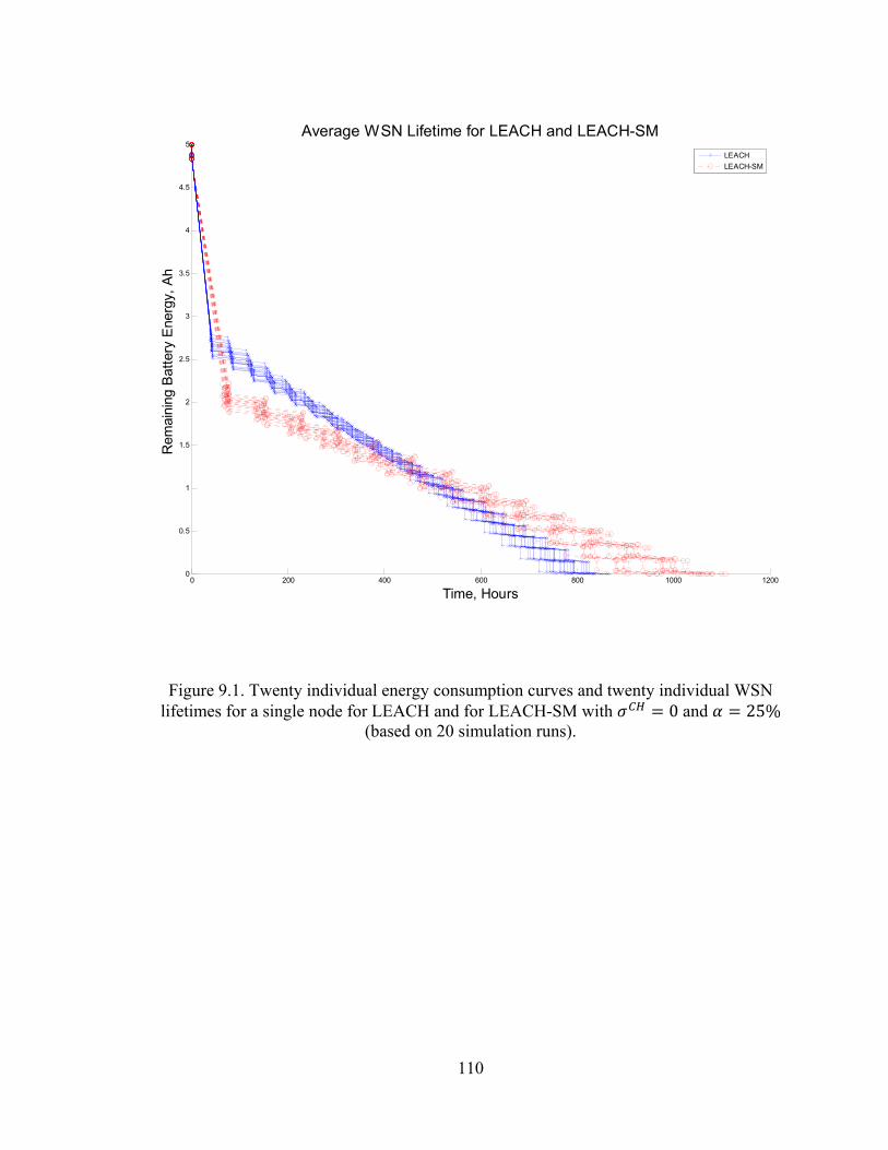
110
0 200 400 600 800 1000 12000
0.5
1
1.5
2
2.5
3
3.5
4
4.5
5
Average WSN Lifetime for LEACH and LEACH-SM
Time, Hours
Rem
aini
ng B
atte
ry E
nerg
y, A
h
LEACH
LEACH-SM
Figure 9.1. Twenty individual energy consumption curves and twenty individual WSN lifetimes for a single node for LEACH and for LEACH-SM with 0 and 25%
(based on 20 simulation runs).

111
0 200 400 600 800 1000 12000
0.5
1
1.5
2
2.5
3
3.5
4
4.5
5
Average WSN Lifetime for LEACH and LEACH-SM
Time, Hours
Rem
aini
ng B
atte
ry E
nerg
y, A
h
LEACH
LEACH-SM
2 1 0
3 4 5 6
Figure 9.2. Average energy consumption curves and average WSN lifetimes for a single node for LEACH and LEACH-SM with 0 and 25% (based on 20 simulation
runs).
In both protocols, each node serves as a cluster head only once in its lifetime. This
period of cluster head service corresponds to the steepest (initial) segment of each energy
consumption curve.
The range of WSN lifetimes for LEACH is from 743 h to 855 h, and the range of
WSN lifetimes for LEACH-SM is from 900 h to 1100 h. This means that the worst case
of WSN lifetime for LEACH-SM is 6% better than the best case of WSN lifetime for

112
LEACH. However, the best case of WSN lifetime for LEACH-SM is 29% better than the
best case of WSN lifetime for LEACH.
Figure 9.2 shows energy consumption curves and average WSN lifetime for a
single node for LEACH and LEACH-SM with 0 and 25%. For LEACH,
[0, is the setup interval for a selected node in LEACH, [ , is the interval when the
node serves as a cluster head in LEACH, and [ , is the interval when the node serves
as a primary in LEACH. For LEACH-SM, [ , is the setup interval for a selected
node, [ , is the spare selection phase, [ , is the interval when the node serves as a
cluster head, and [ , is the interval when the node serves as a primary. (Line
fragments parallel to the time axis indicate the nap periods—with no energy
consumption.)
Figure 9.2 shows that a WSN in LEACH-SM can achieve lifetime longer than the
same WSN in LEACH. For the simulated runs, WSN lifetime in LEACH-SM was longer
about 23%.

113
Case 2: 0 and 50%
Figure 9.3 shows twenty individual energy consumption curves and WSN
lifetimes for a single node for LEACH and LEACH-SM with 0 and 50%.
Table A.3 and Table A.4 in Appendix A give the detailed numerical results for these
results of 20 simulation runs.
0 500 1000 15000
0.5
1
1.5
2
2.5
3
3.5
4
4.5
5
Average WSN Lifetime for LEACH and LEACH-SM
Time, Hours
Rem
aini
ng B
atte
ry E
nerg
y, A
h
LEACH
LEACH-SM
Figure 9.3. Twenty individual energy consumption curves and twenty individual WSN lifetimes for a single node for LEACH and for LEACH-SM with 0 and 50%
(based on 20 simulation runs).

114
0 200 400 600 800 1000 1200 14000
0.5
1
1.5
2
2.5
3
3.5
4
4.5
5
Average WSN Lifetime for LEACH and LEACH-SM
Time, Hours
Rem
aini
ng B
atte
ry E
nerg
y, A
h
LEACH
LEACH-SM
2 1 0
3 4 5 6
Figure 9.4. Average energy consumption curves and average WSN lifetimes for a single node for LEACH and LEACH-SM with 0 and 50% (based on 20 simulation
runs).
In both protocols, each node serves as a cluster head only once in its lifetime. This
period of cluster head service corresponds to the steepest (initial) segment of each energy
consumption curve.
The range of WSN lifetimes for LEACH is from 740 h to 850 h, and the range of
WSN lifetimes for LEACH-SM is from 1100 h to 1300 h. This means that the worst case
of WSN lifetime for LEACH-SM is 29% better than the best case of WSN lifetime for

115
LEACH. However, the best case of WSN lifetime for LEACH-SM is 52% better than the
best case of WSN lifetime for LEACH.
Figure 9.4 shows energy consumption curves and average WSN lifetime for a
single node in LEACH and LEACH-SM with 0 and 50%. For LEACH,
[0, is the setup interval for a selected node in LEACH, [ , is the interval when the
node serves as a cluster head in LEACH, and [ , is the interval when the node serves
as a primary in LEACH. For LEACH-SM, [ , is the setup interval for a selected
node, [ , is the spare selection phase, [ , is the interval when the node serves as a
cluster head, and [ , is the interval when the node serves as a primary. (Line
fragments parallel to the time axis indicate the nap periods—with no energy
consumption.)
Figure 9.4 shows that a WSN in LEACH-SM can achieve lifetime longer than the
same WSN in LEACH. For the simulated runs, WSN lifetime in LEACH-SM was longer
about 48%.

116
Case 3: 10 and 25%
Figure 9.5 shows twenty individual energy consumption curves and WSN
lifetimes for a single node for LEACH and LEACH-SM with 10 and 25%.
Table A.5 and Table A.6 in Appendix A give the detailed numerical results for these
results of 20 simulation runs.
0 500 1000 1500 2000 2500 3000 35000
0.5
1
1.5
2
2.5
3
3.5
4
4.5
5
Average WSN Lifetime for LEACH and LEACH-SM
Time, Hours
Rem
aini
ng B
atte
ry E
nerg
y, A
h
LEACH
LEACH-SM
Figure 9.5. Twenty individual energy consumption curves and twenty individual WSN lifetimes for a single node for LEACH and for LEACH-SM with 10 and
25% (based on 20 simulation runs).

117
0 500 1000 1500 2000 2500 30000
0.5
1
1.5
2
2.5
3
3.5
4
4.5
5
Average WSN Lifetime for LEACH and LEACH-SM
Time, Hours
Rem
aini
ng B
atte
ry E
nerg
y, A
h
LEACH
LEACH-SM
2 1 0
3 4 5 6
Figure 9.6. Average energy consumption curves and average WSN lifetimes for a single node for LEACH and LEACH-SM with 10 and 25% (based on 20
simulation runs).
In both protocols, each node serves as a cluster head only once in its lifetime. This
period of cluster head service corresponds to the steepest (initial) segment of each energy
consumption curve.
The range of WSN lifetimes for LEACH is from 2062 h to 2362 h, and the range
of WSN lifetimes for LEACH-SM is from 2569 h to 2769 h. This means that the worst
case of WSN lifetime for LEACH-SM is 8% better than the best case of WSN lifetime

118
for LEACH. However, the best case of WSN lifetime for LEACH-SM is 17% better than
the best case of WSN lifetime for LEACH.
Figure 9.6 shows energy consumption curves and average WSN lifetime for a
single node in LEACH and LEACH-SM with 10 and 25%. For LEACH,
[0, is the setup interval for a selected node in LEACH, [ , is the interval when the
node serves as a cluster head in LEACH, and [ , is the interval when the node serves
as a primary in LEACH. For LEACH-SM, [ , is the setup interval for a selected
node, [ , is the spare selection phase, [ , is the interval when the node serves as a
cluster head, and [ , is the interval when the node serves as a primary. (Line
fragments parallel to the time axis indicate the nap periods—with no energy
consumption.)
Figure 9.6 shows that a WSN in LEACH-SM can achieve lifetime longer than the
same WSN in LEACH. For the simulated runs, WSN lifetime in LEACH-SM was longer
about 23%.

119
Case 4: 10 and 50%
Figure 9.7 shows twenty individual energy consumption curves and WSN
lifetimes for a single node for LEACH and LEACH-SM with 10 and 50%.
Table A.7 and Table A.8 in Appendix A give the detailed numerical results for these
results of 20 simulation runs.
0 500 1000 1500 2000 2500 3000 3500 40000
0.5
1
1.5
2
2.5
3
3.5
4
4.5
5
Average WSN Lifetime for LEACH and LEACH-SM
Time, Hours
Rem
aini
ng B
atte
ry E
nerg
y, A
h
LEACH
LEACH-SM
Figure 9.7. Twenty individual energy consumption curves and twenty individual WSN lifetimes for a single node for LEACH and for LEACH-SM with 10 and
50% (based on 20 simulation runs).

120
0 500 1000 1500 2000 2500 3000 35000
0.5
1
1.5
2
2.5
3
3.5
4
4.5
5
Average WSN Lifetime for LEACH and LEACH-SM
Time, Hours
Rem
aini
ng B
atte
ry E
nerg
y, A
h
LEACH
LEACH-SM
2 1 0
3 4 5 6
Figure 9.8. Average energy consumption curves and average WSN lifetimes for a single node for LEACH and LEACH-SM with 10 and 50% (based on 20
simulation runs).
In both protocols, each node serves as a cluster head only once in its lifetime. This
period of cluster head service corresponds to the steepest (initial) segment of each energy
consumption curve.
The range of WSN lifetimes for LEACH is from 2062 h to 2362 h, and the range
of WSN lifetimes for LEACH-SM is from 3106 h to 3306 h. This means that the worst
case of WSN lifetime for LEACH-SM is 31% better than the best case of WSN lifetime

121
for LEACH. However, the best case of WSN lifetime for LEACH-SM is 40% better than
the best case of WSN lifetime for LEACH.
Figure 9.8 shows energy consumption curves and average WSN lifetime for a
single node in LEACH and LEACH-SM with 10 and 50%. For LEACH,
[0, is the setup interval for a selected node in LEACH, [ , is the interval when the
node serves as a cluster head in LEACH, and [ , is the interval when the node serves
as a primary in LEACH. For LEACH-SM, [ , is the setup interval for a selected
node, [ , is the spare selection phase, [ , is the interval when the node serves as a
cluster head, and [ , is the interval when the node serves as a primary. (Line
fragments parallel to the time axis indicate the nap periods—with no energy
consumption.)
Figure 9.8 shows that a WSN in LEACH-SM can achieve lifetime longer than the
same WSN in LEACH. For the simulated runs, WSN lifetime in LEACH-SM was longer
about 48%.

122
Case 5: 20 and 25%
Figure 9.9 shows twenty individual energy consumption curves and WSN
lifetimes for a single node for LEACH and LEACH-SM with 20 and 25%.
Table A.9 and Table A.10 in Appendix A give the detailed numerical results for these
results of 20 simulation runs.
0 500 1000 1500 2000 2500 3000 3500 4000 4500 50000
0.5
1
1.5
2
2.5
3
3.5
4
4.5
5
Average WSN Lifetime for LEACH and LEACH-SM
Time, Hours
Rem
aini
ng B
atte
ry E
nerg
y, A
h
LEACH
LEACH-SM
Figure 9.9. Twenty individual energy consumption curves and twenty individual WSN lifetimes for a single node for LEACH and for LEACH-SM with 20 and
25% (based on 20 simulation runs).

123
0 500 1000 1500 2000 2500 3000 3500 4000 45000
0.5
1
1.5
2
2.5
3
3.5
4
4.5
5
Average WSN Lifetime for LEACH and LEACH-SM
Time, Hours
Rem
aini
ng B
atte
ry E
nerg
y, A
h
LEACH
LEACH-SM
2 1 0
3 4 5 6
Figure 9.10. Average energy consumption curves and average WSN lifetimes for a single node for LEACH and LEACH-SM with 20 and 25% (based on 20
simulation runs).
In both protocols, each node serves as a cluster head only once in its lifetime. This
period of cluster head service corresponds to the steepest (initial) segment of each energy
consumption curve.
The range of WSN lifetimes for LEACH is from 3410 h to 3610 h, and the range
of WSN lifetimes in LEACH-SM is from 4227 h to 4427 h. This means that the worst
case of WSN lifetime for LEACH-SM is 17% better than the best case of WSN lifetime
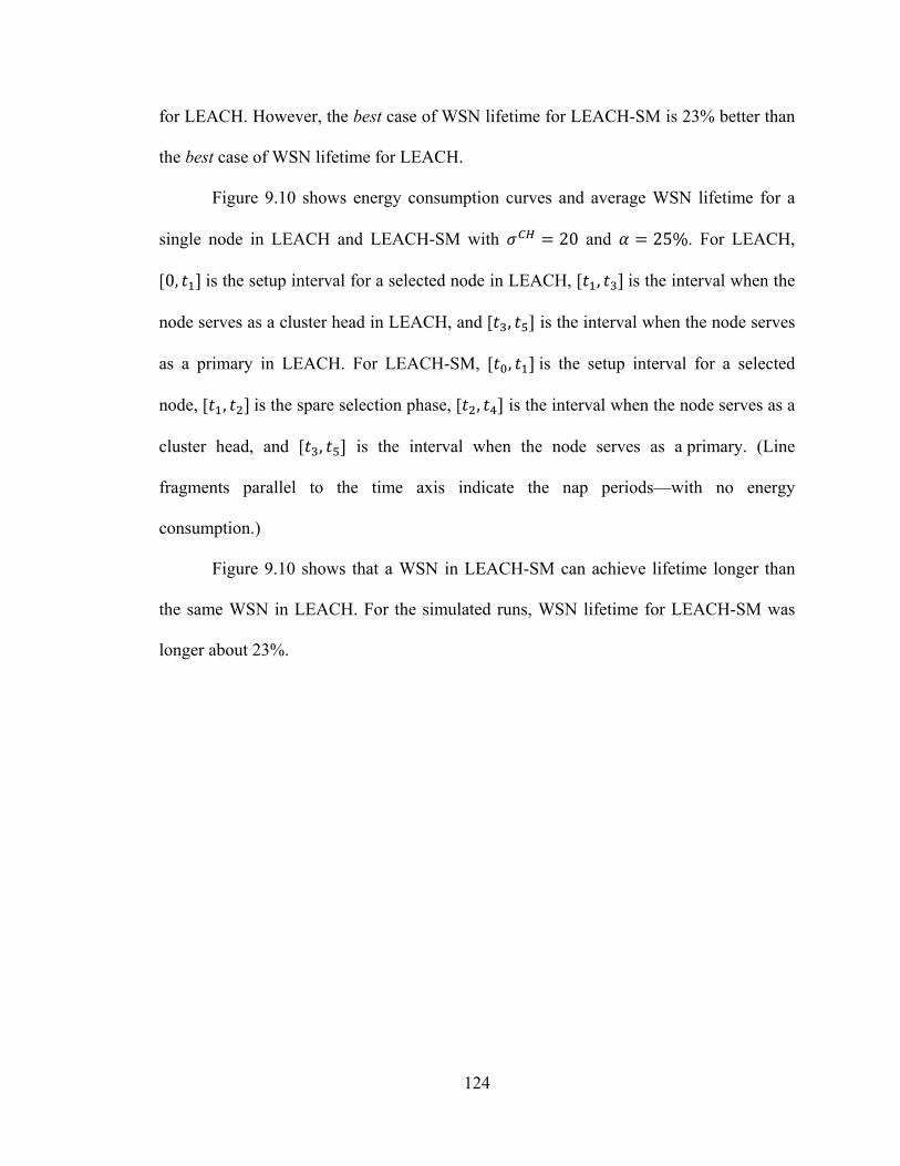
124
for LEACH. However, the best case of WSN lifetime for LEACH-SM is 23% better than
the best case of WSN lifetime for LEACH.
Figure 9.10 shows energy consumption curves and average WSN lifetime for a
single node in LEACH and LEACH-SM with 20 and 25%. For LEACH,
[0, is the setup interval for a selected node in LEACH, [ , is the interval when the
node serves as a cluster head in LEACH, and [ , is the interval when the node serves
as a primary in LEACH. For LEACH-SM, [ , is the setup interval for a selected
node, [ , is the spare selection phase, [ , is the interval when the node serves as a
cluster head, and [ , is the interval when the node serves as a primary. (Line
fragments parallel to the time axis indicate the nap periods—with no energy
consumption.)
Figure 9.10 shows that a WSN in LEACH-SM can achieve lifetime longer than
the same WSN in LEACH. For the simulated runs, WSN lifetime for LEACH-SM was
longer about 23%.

125
Case 6: 20 and 50%
Figure 9.11 shows twenty individual energy consumption curves and WSN
lifetimes for a single node for LEACH and LEACH-SM with 20 and 50%.
Table A.11 and Table A.12 in Appendix A give the detailed numerical results for these
results of 20 simulation runs.
0 1000 2000 3000 4000 5000 6000 70000
0.5
1
1.5
2
2.5
3
3.5
4
4.5
5
Average WSN Lifetime for LEACH and LEACH-SM
Time, Hours
Rem
aini
ng B
atte
ry E
nerg
y, A
h
LEACH
LEACH-SM
Figure 9.11. Twenty individual energy consumption curves and twenty individual WSN lifetimes for a single node for LEACH and for LEACH-SM with 20 and
50% (based on 20 simulation runs).

126
0 1000 2000 3000 4000 5000 60000
0.5
1
1.5
2
2.5
3
3.5
4
4.5
5
Average WSN Lifetime for LEACH and LEACH-SM
Time, Hours
Rem
aini
ng B
atte
ry E
nerg
y, A
h
LEACH
LEACH-SM
2 1 0
3 4 5 6
Figure 9.12. Average energy consumption curves and average WSN lifetimes for a single node for LEACH and LEACH-SM with 20 and 50% (based on 20
simulation runs).
In both protocols, each node serves as a cluster head only once in its lifetime. This
period of cluster head service corresponds to the steepest (initial) segment of each energy
consumption curve.
The range of WSN lifetimes for LEACH is from 3410 h to 3610 h, and the range
of WSN lifetimes in LEACH-SM is from 5128 h to 5328 h. This means that the worst
case of WSN lifetime for LEACH-SM is 42% better than the best case of WSN lifetime

127
for LEACH. However, the best case of WSN lifetime for LEACH-SM is 47% better than
the best case of WSN lifetime for LEACH.
Figure 9.12 shows energy consumption curves and average WSN lifetime for a
single node for LEACH and LEACH-SM with 20 and 50%. For LEACH,
[0, is the setup interval for a selected node in LEACH, [ , is the interval when the
node serves as a cluster head in LEACH, and [ , is the interval when the node serves
as a primary in LEACH. For LEACH-SM, [ , is the setup interval for a selected
node, [ , is the spare selection phase, [ , is the interval when the node serves as a
cluster head, and [ , is the interval when the node serves as a primary. (Line
fragments parallel to the time axis indicate the nap periods—with no energy
consumption.)
Figure 9.12 shows that a WSN in LEACH-SM can achieve lifetime longer than
the same WSN in LEACH. For the simulated runs, WSN lifetime in LEACH-SM was
longer about 48%.

128
Case 7: 30 and 25%
Figure 9.13 shows twenty individual energy consumption curves and WSN
lifetimes for a single node for LEACH and LEACH-SM with 30 and 25%.
Table A.13 and Table A.14 in Appendix A give the detailed numerical results for these
results of 20 simulation runs.
0 1000 2000 3000 4000 5000 6000 70000
0.5
1
1.5
2
2.5
3
3.5
4
4.5
5
Average WSN Lifetime for LEACH and LEACH-SM
Time, Hours
Rem
aini
ng B
atte
ry E
nerg
y, A
h
LEACH
LEACH-SM
Figure 9.13. Twenty individual energy consumption curves and twenty individual WSN lifetimes for a single node for LEACH and for LEACH-SM with 30 and
25% (based on 20 simulation runs).

129
0 1000 2000 3000 4000 5000 60000
0.5
1
1.5
2
2.5
3
3.5
4
4.5
5
Average WSN Lifetime for LEACH and LEACH-SM
Time, Hours
Rem
aini
ng B
atte
ry E
nerg
y, A
h
LEACH
LEACH-SM
2 1 0
3 4 5 6
Figure 9.14. Average energy consumption curves and average WSN lifetimes for a single node for LEACH and LEACH-SM with 30 and 25% (based on 20
simulation runs).
In both protocols, each node serves as a cluster head only once in its lifetime. This
period of cluster head service corresponds to the steepest (initial) segment of each energy
consumption curve.
The range of WSN lifetimes for LEACH is from 4756 h to 4956 h, and the range
of WSN lifetimes in LEACH-SM is from 5888 h to 8088 h. This means that the worst

130
case of WSN lifetime for LEACH-SM is 18% better than the best case of WSN lifetime
for LEACH. However, the best case of WSN lifetime for LEACH-SM is 63% better than
the best case of WSN lifetime for LEACH.
Figure 9.14 shows energy consumption curves and average WSN lifetime for a
single node for LEACH and LEACH-SM with 30 and 25%. For LEACH,
[0, is the setup interval for a selected node in LEACH, [ , is the interval when the
node serves as a cluster head in LEACH, and [ , is the interval when the node serves
as a primary in LEACH. For LEACH-SM, [ , is the setup interval for a selected
node, [ , is the spare selection phase, [ , is the interval when the node serves as a
cluster head, and [ , is the interval when the node serves as a primary. (Line
fragments parallel to the time axis indicate the nap periods—with no energy
consumption.)
Figure 9.14 shows that a WSN in LEACH-SM can achieve lifetime longer than
the same WSN in LEACH. For the simulated runs, WSN lifetime in LEACH-SM was
longer about 23%.

131
Case 8: 30 and 50%
Figure 9.15 shows twenty individual energy consumption curves and WSN
lifetimes for a single node for LEACH and LEACH-SM with 30 and 50%.
Table A.15 and Table A.16 in Appendix A give the detailed numerical results for these
results of 20 simulation runs.
0 1000 2000 3000 4000 5000 6000 7000 8000 90000
0.5
1
1.5
2
2.5
3
3.5
4
4.5
5
Average WSN Lifetime for LEACH and LEACH-SM
Time, Hours
Rem
aini
ng B
atte
ry E
nerg
y, A
h
LEACH
LEACH-SM
Figure 9.15. Twenty individual energy consumption curves and twenty individual WSN lifetimes for a single node for LEACH and for LEACH-SM with 30 and
50% (based on 20 simulation runs).

132
0 1000 2000 3000 4000 5000 6000 7000 80000
0.5
1
1.5
2
2.5
3
3.5
4
4.5
5
Average WSN Lifetime for LEACH and LEACH-SM
Time, Hours
Rem
aini
ng B
atte
ry E
nerg
y, A
h
LEACH
LEACH-SM
2 1 0
3 4 5 6
Figure 9.16. Average energy consumption curves and average WSN lifetimes for a single node for LEACH and LEACH-SM with 30 and 50% (based on 20
simulation runs).
In both protocols, each node serves as a cluster head only once in its lifetime. This
period of cluster head service corresponds to the steepest (initial) segment of each energy
consumption curve.
The range of WSN lifetimes for LEACH is from 4756 h to 4956 h, and the range
of WSN lifetimes in LEACH-SM is from 7100 h to 7300 h. This means that the worst

133
case of WSN lifetime for LEACH-SM is 43% better than the best case of WSN lifetime
for LEACH. However, the best case of WSN lifetime for LEACH-SM is 47% better than
the best case of WSN lifetime for LEACH.
Figure 9.16 shows energy consumption curves and average WSN lifetime for a
single node for LEACH and LEACH-SM with 30 and 50%. For LEACH,
[0, is the setup interval for a selected node in LEACH, [ , is the interval when the
node serves as a cluster head in LEACH, and [ , is the interval when the node serves
as a primary in LEACH. For LEACH-SM, [ , is the setup interval for a selected
node, [ , is the spare selection phase, [ , is the interval when the node serves as a
cluster head, and [ , is the interval when the node serves as a primary. (Line
fragments parallel to the time axis indicate the nap periods—with no energy
consumption.)
Figure 9.16 shows that a WSN in LEACH-SM can achieve lifetime longer than
the same WSN in LEACH. For the simulated runs, WSN lifetime in LEACH-SM was
longer about 48%.
9.5.1.2 Simulation Results for Ranges of σ or α Values
We consider here six cases with different combinations of values for
(duration of a nap interval for a cluster head) and (spare ratio)—as shown in Table 9.5.

134
Table 9.5. Comparison of LEACH-SM with LEACH.
Case
Number
Duration(s) of a
nap interval for
a cluster head
(
The spare
ratio(s) for
LEACH-SM
( )
Figures Tables
1. 0, 10, 20, 30 25% Figure 9.17
Table A.1
Table A.2
Table A.5
Table A.6
Table A.9
Table A.10
Table A.13
Table A.14
2. 0, 10, 20, 30 50% Figure 9.18
Table A.3
Table A.4
Table A.7
Table A.8
Table A.11
Table A.12
Table A.15
Table A.16

135
Table 9.5 – Continued
3. 0 25%, 50% Figure 9.19
Table A.1
Table A.2
Table A.3
Table A.4
4. 10 25%, 50% Figure 9.20
Table A.5
Table A.6
Table A.7
Table A.8
5. 20 25%, 50% Figure 9.21
Table A.9
Table A.10
Table A.11
Table A.12
6. 30 25%, 50% Figure 9.22
Table A.13
Table A.14
Table A.15
Table A.16

136
Case 1: 0,10, 20, 30 and 25%
Figure 9.17, shows eight individual energy consumption curves and WSN
lifetimes for a single node for LEACH and LEACH-SM with 0, 10, 20, 30 and
25%.
0 1000 2000 3000 4000 5000 60000
0.5
1
1.5
2
2.5
3
3.5
4
4.5
5
Average WSN Lifetime for LEACH and LEACH-SM with increasing Nap interval
Time, Hours
Rem
aini
ng B
atte
ry E
nerg
y, A
h
LEACH
LEACH-SM
0 LEACHLEACH-SM
10
20 30
LEACHLEACH-SM
LEACHLEACH-SM LEACH
LEACH-SM
Figure 9.17. Average energy consumption curves and average WSN lifetimes for a single node for LEACH and LEACH-SM for parameter values: 0, 10, 20, 30 and
25%.

137
In both protocols, each node serves as a cluster head only once in its lifetime. This
period of cluster head service corresponds to the steepest (initial) segment of each energy
consumption curve.
WSN lifetime in LEACH-SM is 23% better than WSN lifetime in LEACH for all
four combinations of values for and (cf. Figure 9.17).
Case 2: 0, 10, 20, 30 and 50%
Figure 9.18, shows eight individual energy consumption curves and WSN
lifetimes for a single node for LEACH and LEACH-SM with 0, 10, 20, 30 and
50%.

138
0 1000 2000 3000 4000 5000 6000 7000 80000
0.5
1
1.5
2
2.5
3
3.5
4
4.5
5
Average WSN Lifetime for LEACH and LEACH-SM with increasing Nap interval
Time, Hours
Rem
aini
ng B
atte
ry E
nerg
y, A
h
LEACH
LEACH-SM
0 10
20 30
Figure 9.18. Average energy consumption curves and average WSN lifetimes for a single node for LEACH and LEACH-SM for
parameter values: 0, 10, 20, 30 and 50%.
WSN lifetime for LEACH-SM is 48% better than the WSN lifetime for LEACH
for all four combinations of values for and (cf. Figure 9.18).
Note that in Figure 9.17 and Figure 9.18, the comparison results give the lower
bound on the WSN lifetime extension provided by LEACH-SM. The reason is that for
LEACH-SM we consider the minimum number of primary nodes and no spares. The

139
Figure 9.17 summarizes only 4 of 8 cases, those with 25% shown in Table 9.4. In
this experiment we increase the Nap interval. At the beginning the value of the Nap
interval is set to zero, that is, the duty cycle for cluster head in LEACH is 100%. In
general, the duty cycle of cluster head in LEACH-SM is decreased by %. We increased
the Nap interval from 0 to 30 with step size of 10 each iteration until the duty cycle is
15%.
We observe that WSN lifetime for LEACH-SM is 23% better than the WSN
lifetime for LEACH for all four combinations of values for and .
Figure 9.18 summarizes the remaining 4 cases, those with 50%, as shown in
Table 9.4. As we did before in this experiment, at the beginning we set the value of the
Nap interval to zero, that is, the duty cycle for LEACH is 100%. In this case =50%.
After that we increased the Nap interval at each iteration up to 30.
WSN lifetime in LEACH-SM is 48% and is better than WSN lifetime in LEACH,
which is 23% for all four combinations of values for and .

140
Case 3: 0 and 25%, 50%
Figure 9.19, shows only three individual energy consumption curves and WSN
lifetimes for a single node for LEACH and LEACH-SM with 0 and
25% 50%.
0 200 400 600 800 1000 1200 14000
0.5
1
1.5
2
2.5
3
3.5
4
4.5
5Average WSN Lifetime for LEACH and LEACH-SM with increasing ratio of the nodes that become spares
Time, Hours
Rem
aini
ng B
atte
ry E
nerg
y, A
h
LEACH
LEACH-SM
25%, 50%
25% 50%
Figure 9.19. Average energy consumption curves and average WSN lifetimes for a single node for LEACH and LEACH-SM for
parameter values: 0 and 25%, 50%.

141
In Figure 9.19, we fixed Nap interval of cluster head and change the spare ratio
from 25% to 50%. As expected, there is no change in WSN lifetime for LEACH,
because LEACH does not use spares. However, a significant increase in WSN lifetime is
observed for LEACH-SM.
WSN lifetime for LEACH-SM is 23% better than the WSN lifetime for LEACH
for 0 and 25%. We observe that WSN lifetime for LEACH-SM is 48% better
than the WSN lifetime for LEACH when we set 0 and 50%.
The Figure 9.19 is in fact summarizes only 2 of 8 cases, those with 0
shown in Table 9.4. In this experiment we increase the spare ratio from 25% to 50% and
fixed Nap interval for cluster head ( ). Since 0, this means that the duty cycle
for LEACH is 100% for both iterations. If =25% of the sensor node are in passive mode
(by using DESST), then the duty cycle of cluster head is decreased by % in LEACH-
SM. That is why WSN lifetime for LEACH-SM is 23% better than the WSN lifetime for
LEACH.
In second iteration for = 50%, we again set 0,which implies that the
duty cycle of cluster head is 100% for LEACH. Therefore, the duty cycle of cluster head
in LEACH-SM is decreased by %. This results in extension of WSN lifetime by 48%
compared to LEACH.
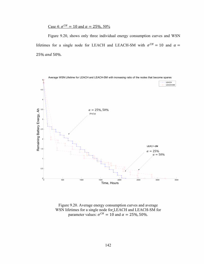
142
Case 4: 10 and 25%, 50%
Figure 9.20, shows only three individual energy consumption curves and WSN
lifetimes for a single node for LEACH and LEACH-SM with 10 and
25% 50%.
0 500 1000 1500 2000 2500 3000 35000
0.5
1
1.5
2
2.5
3
3.5
4
4.5
5Average WSN Lifetime for LEACH and LEACH-SM with increasing ratio of the nodes that become spares
Time, Hours
Rem
aini
ng B
atte
ry E
nerg
y, A
h
LEACH
LEACH-SM
25%, 50%
25% 50%
Figure 9.20. Average energy consumption curves and average WSN lifetimes for a single node for LEACH and LEACH-SM for
parameter values: 10 and 25%, 50%.

143
In Figure 9.20, we fixed Nap interval of cluster head and change the spare ratio
from 25% to 50%. As expected there is no change in WSN lifetime for LEACH,
because LEACH does not use spares. However increase in WSN lifetime significantly
observed in LEACH-SM.
WSN lifetime for LEACH-SM is 23% better than the WSN lifetime for LEACH
for 10 and 25%. We observe that WSN lifetime for LEACH-SM is 48%
better than the WSN lifetime for LEACH when we set 10 and 50%.
The Figure 9.20 is in fact summarizes only 2 of 8 cases, those with 10
shown in Table 9.4. In this experiment we increase the spare ratio from 25% to 50% and
fixed Nap interval for cluster head ( ). Since 10, this means that the duty cycle
for LEACH is 37% for both iterations. If =25% of the sensor node are in passive mode
(by using DESST), then the duty cycle of cluster head in LEACH-SM is only 27%. That
is why WSN lifetime for LEACH-SM is 23% better than the WSN lifetime for LEACH.
In second iteration for =50%, we set 0, which implies that the duty cycle
of cluster head is 37% for LEACH. The duty cycle of cluster head in LEACH-SM is
17%. This results in extension of WSN lifetime by 48% compared to LEACH.

144
Case 5: 20 and 25%, 50
Figure 9.21, shows only three individual energy consumption curves and WSN
lifetimes for a single node for LEACH and LEACH-SM with 20 and
25% 50%.
0 1000 2000 3000 4000 5000 60000
0.5
1
1.5
2
2.5
3
3.5
4
4.5
5Average WSN Lifetime for LEACH and LEACH-SM with increasing ratio of the nodes that become spares
Time, Hours
Rem
aini
ng B
atte
ry E
nerg
y, A
h
LEACH
LEACH-SM
25%, 50% LEACH
LEACH-SM
25% 50%
Figure 9.21. Average energy consumption curves and average WSN lifetimes for a single node for LEACH and LEACH-SM for
parameter values: 20 and 25%, 50%.
In Figure 9.21, we fixed Nap interval of cluster head and change the spare ratio
from 25% to 50%. As expected there is no change in WSN lifetime for LEACH,

145
because LEACH does not use spares. However, significant increase in WSN lifetime is
observed in LEACH-SM.
WSN lifetime for LEACH-SM is 23% better than WSN lifetime for LEACH for
20 and 25%. We observe that WSN lifetime for LEACH-SM is 48% better
than WSN lifetime for LEACH when we set 20 and 50%.
The Figure 2.1 summarizes only 2 of 8 cases, namely those with 20 as
shown in Table 9.4. In this experiment we increase the spare ratio from 25% to 50% and
fix Nap interval for cluster head ( ).
In the first case, =25% and 20. The duty cycle of cluster head for
LEACH is 23%. The duty cycle of cluster head for LEACH-SM is only 17%, which is
significantly lower than 23% for LEACH. WSN lifetime for LEACH-SM is 23%
(coincidentally also 23%) longer than WSN lifetime for LEACH.
In the second case, =50% and 20. The duty cycle of cluster head for
LEACH is again 23%. The duty cycle of cluster head in LEACH-SM is only 11%. WSN
lifetime for LEACH-SM is 48% longer than WSN lifetime for LEACH.

146
Case 6: 30 and 25%, 50
Figure 9.22, shows only three individual energy consumption curves and WSN
lifetimes for a single node for LEACH and LEACH-SM with 30 and
25% 50%..
0 1000 2000 3000 4000 5000 6000 7000 80000
0.5
1
1.5
2
2.5
3
3.5
4
4.5
5Average WSN Lifetime for LEACH and LEACH-SM with increasing ratio of the nodes that become spares
Time, Hours
Rem
aini
ng B
atte
ry E
nerg
y, A
h
LEACH
LEACH-SM
25%, 50%
25% 50%
Figure 9.22. Average energy consumption curves and average WSN lifetimes for a single node for LEACH and LEACH-SM for
parameter values: 30 and 25%, 50%.
In Figure 9.22, we fixed Nap interval of cluster head and change the spare ratio
from 25% to 50%. As expected there is no change in WSN lifetime for LEACH,

147
because LEACH does not use spares. However, significant increase in WSN lifetime is
observed in LEACH-SM.
WSN lifetime for LEACH-SM is 23% better than WSN lifetime for LEACH for
20 and 25%. We observe that WSN lifetime for LEACH-SM is 48% better
than WSN lifetime for LEACH when we set 20 and 50%.
The Figure 2.1 summarizes only 2 of 8 cases, namely those with 30 as
shown in Table 9.4. In this experiment we increase the spare ratio from 25% to 50% and
fix Nap interval for cluster head ( ).
In the first case, =25% and 30. The duty cycle of cluster head for
LEACH is 17%. The duty cycle of cluster head for LEACH-SM is only 12%, which is
significantly lower than 23% for LEACH. WSN lifetime for LEACH-SM is 23%
(coincidentally also 23%) longer than WSN lifetime for LEACH.
In the second case, =50% and 30. The duty cycle of cluster head for
LEACH is again 23%. The duty cycle of cluster head in LEACH-SM is only 12%. WSN
lifetime for LEACH-SM is 48% longer than WSN lifetime for LEACH.
9.5.2 ResultsofEnergyConsumptionandWSNLifetimeSimulationsforLEACH‐SMwithSpareReplacements
This section presents the results of energy consumption and WSN lifetime
simulation for LEACH-SM with spare replacement. The first subsection shows
simulation results for individual combinations of values for (duration of a nap
interval for a cluster head) and (spare ratio), while the second subsection shows
simulation results for ranges of or values.

148
9.5.2.1 Simulation Results for Individual Combinations of σ and α Values
Each replacement assures that WSN using LEACH-SM continues to live (without
a next spare available, WSN would die if its coverage goes below the required minimum
coverage). Note that each consecutive addition extends WSN lifetime by a smaller period
(since a spare that waits for a longer time to become a primary uses more of its energy
during its Awake-Nap cycles executed before becoming a primary).
There are no spares in LEACH. When a primary dies at time there is no
replacement for it. Therefore, WSN can achieve longer lifetime if it uses LEACH-SM
rather than LEACH.
For better understanding of the replacement process in LEACH-SM, let us
consider the example.
Example: Replacement Process in LEACH-SM
Let us consider only two simple cases. We assume one cluster for the sake of
simplicity. We also assume that the number of nodes remains fixed after each setup
phase. Finally, we assume that there are 20 nodes in this cluster.
Case 1: 25%
To maintain the above-threshold target coverage let us assume that the spare ratio
is 25%. Then, we have 5 spares and 15 primaries (including cluster head), as shown in
Figure 9.23.

149
Figure 9.23. Illustration of a cluster with 20 nodes and 25%.
Recall that LEACH and LEACH-SM balance energy usage by a node in such a
way that all initial primaries and cluster head die at nearly the same time. We simulate
one node which starts as a cluster head. Other nodes behaves analogously (with the
difference that they serve as a cluster head in different rounds).
In this case 15 nodes die nearly at the same time denoted as . In Case 1
LEACH-SM attempts to replace all 15 primary nodes (including 1 cluster head and 14
regular nodes) as shown in Figure 9.23. However we have only 5 spares, so the
replacement of 15 primary nodes is not possible. Therefore WSN dies at .

150
Case 2: 50%
In this case, have 10 active nodes (incl. cluster head) and 10 spares as shown in
Figure 9.24.
Figure 9.24. Illustration of a cluster with 20 nodes and 50% at the deployment time.

151
Figure 9.25. Illustration for a cluster with 20 nodes and 50% after the first replacement at time .
All primaries die simultaneously at time . Figure 9.24 shows that we have 10
spare nodes available. Therefore in this case the first replacement is possible. After the
first replacement, we have 10 primaries (including cluster head) and 0 spares as shown in
Figure 9.25.
At time , all primaries die simultaneously. We have no spares to replace them,
so WSN dies as well.
Figure 9.25 shows that we have 0 spares available at time . Therefore, in this
case the second replacement is not possible.

152
Table 9.6. Cases to measure WSN lifetime when replacements of exhausted primary nodes by spares are allowed.
Sr.
Duration of a
nap interval of
a cluster head
(
The spare ratio(s)
for LEACH-SM
( )
Figures Tables
1. 0 50% Figure 9.26,
Figure 9.27 Table A.4
2. 10 50% Figure 9.28,
Figure 9.29 Table A.8
3. 20 50%
Figure 9.30,
Figure 9.31
Table A.12
4. 30 50% Figure 9.32,
Figure 9.33 Table A.16
It is clear from the above example that the replacement process is possible only if
the spare ratio is 50% or more provided all spares are able to cover the targets covered by
primaries that exhausted their energy.
We consider here 4 cases with different combinations of values for (duration
of a nap interval for a cluster head) and 50% (spare ratio)—as shown in Table 9.6.
Since we consider WSN lifetimes when spare replacements of exhausted primaries are
allowed, there are no results for LEACH (because LEACH uses no spares).
153
Each former spare that became a primary is in turn replaced by another spare
when its energy is exhausted. Each replacement assures that WSN continues to live
(without a next spare available, WSN would die if its target coverage goes below the
required minimum coverage).
Case 1: 0 and 50%
Figure 9.26 and Figure 9.27 shows energy consumption curves for an exhausted
primary, and a spare that replaced it. More precisely, the first of these figures shows
results of 20 simulation runs; it shows twenty individual energy consumption curves and
twenty individual WSN lifetimes for a single node for LEACH-SM with 0 and
50%. Table A.18 in Appendix A gives the detailed numerical results for these 20
runs.
Figure 9.27 shows the average WSN lifetimes and the energy consumption curves
for an exhausted primary, and a spare that replaced it. At time , the primary dies, and
is replaced by spare , which already used up 5 of its energy (as shown by the blue
curve). After time , is a primary and consumes more energy, as shown by the steeper
red curve.

154
0 1000 2000 3000 4000 5000 6000 7000 80000
0.5
1
1.5
2
2.5
3
3.5
4
4.5
5
Average WSN Lifetime for LEACH-SM
Time, Hours
Rem
aini
ng B
atte
ry E
nerg
y, A
h
Primary
Spare
These curve segments represents
how spares (if any were left would use
their energy)
Figure 9.26. Twenty individual energy consumption curves and twenty individual WSN lifetimes for a single node for LEACH-SM with 0 and 50% (based on 20
simulation runs).

155
0 1000 2000 3000 4000 5000 6000 70000
0.5
1
1.5
2
2.5
3
3.5
4
4.5
5
Average WSN Lifetime for LEACH-SM
Time, Hours
Rem
aini
ng B
atte
ry E
nerg
y, A
h
Primary
Spare
1
1
Figure 9.27. Average WSN lifetime for LEACH-SM with 0 and 50%. The energy consumption curves for an exhausted primary, and a spare that replaced it.

156
Case 2: 10 and 50%
Figure 9.28 and Figure 9.29 shows energy consumption curves for an exhausted
primary, and a spare that replaced it. More precisely, the first of these figures shows
results of 20 simulation runs; it shows twenty individual energy consumption curves and
twenty individual WSN lifetimes for a single node for LEACH-SM with 10 and
50%. Table A.20 in Appendix A gives the detailed numerical results for these 20
runs.
Figure 9.29 shows the average WSN lifetimes and the energy consumption curves
for an exhausted primary, and a spare that replaced it. At time , the primary dies, and
is replaced by spare , which already used up 5 of its energy (as shown by the blue
curve). After time , is a primary and consumes more energy, as shown by the steeper
red curve.

157
0 0.2 0.4 0.6 0.8 1 1.2 1.4 1.6 1.8 2
x 104
0
0.5
1
1.5
2
2.5
3
3.5
4
4.5
5
Average WSN Lifetime for LEACH-SM
Time, Hours
Rem
aini
ng B
atte
ry E
nerg
y, A
h
Primary
Spare
These curve segments represents
how spares (if any were left would use
their energy)
Figure 9.28. Twenty individual energy consumption curves and twenty individual WSN lifetimes for a single node for LEACH-SM with 10 and 50% (based on 20
simulation runs).

158
0 0.2 0.4 0.6 0.8 1 1.2 1.4 1.6 1.8 2
x 104
0
0.5
1
1.5
2
2.5
3
3.5
4
4.5
5
Average WSN Lifetime for LEACH-SM
Time, Hours
Rem
aini
ng B
atte
ry E
nerg
y, A
h
Primary
Spare
1
1
These curve segments represents
how spares (if any were left would use
their energy)
Figure 9.29. Average WSN lifetime for LEACH-SM with 10 and 50%.
Case 3: 20 and 50%
Figure 9.30 and Figure 9.31 shows energy consumption curves for an exhausted
primary, and a spare that replaced it. More precisely, the first of these figures shows
results of 20 simulation runs; it shows twenty individual energy consumption curves and
twenty individual WSN lifetimes for a single node for LEACH-SM with 20 and

159
50%. Table A.22 in Appendix A gives the detailed numerical results for these 20
runs.
Figure 9.31 shows the average WSN lifetimes and the energy consumption curves
for an exhausted primary, and a spare that replaced it. At time , the primary dies, and
is replaced by spare , which already used up 5 of its energy (as shown by the blue
curve). After time , is a primary and consumes more energy, as shown by the steeper
red curve.

160
0 0.5 1 1.5 2 2.5 3 3.5
x 104
0
0.5
1
1.5
2
2.5
3
3.5
4
4.5
5
Average WSN Lifetime for LEACH-SM
Time, Hours
Rem
aini
ng B
atte
ry E
nerg
y, A
h
Primary
Spare
Figure 9.30. Twenty individual energy consumption curves and twenty individual WSN lifetimes for a single node for LEACH-SM with 20 and 50% (based on 20
simulation runs).

161
0 0.5 1 1.5 2 2.5 3
x 104
0
0.5
1
1.5
2
2.5
3
3.5
4
4.5
5
Average WSN Lifetime for LEACH-SM
Time, Hours
Rem
aini
ng B
atte
ry E
nerg
y, A
h
Primary
Spare
1
1
These curve segments represents
how spares (if any were left would use
their energy)
Figure 9.31. Average WSN lifetime for LEACH-SM with 20 and 50%.
Case 4: 30 and 50%
Figure 9.32 and Figure 9.33 shows energy consumption curves for an exhausted
primary, and a spare that replaced it. More precisely, the first of these figures shows
results of 20 simulation runs; it shows twenty individual energy consumption curves and
twenty individual WSN lifetimes for a single node for LEACH-SM with 30 and
50%. Table A.24 in Appendix A gives the detailed numerical results for these 20
runs.

162
Figure 9.33 shows the average WSN lifetimes and the energy consumption curves
for an exhausted primary, and a spare that replaced it. At time , the primary dies, and
is replaced by spare , which already used up 5 of its energy (as shown by the blue
curve). After time , is a primary and consumes more energy, as shown by the steeper
red curve.
0 0.5 1 1.5 2 2.5 3 3.5 4 4.5
x 104
0
0.5
1
1.5
2
2.5
3
3.5
4
4.5
5
Average WSN Lifetime for LEACH-SM
Time, Hours
Rem
aini
ng B
atte
ry E
nerg
y, A
h
Primary
Spare
These curve segments represents
how spares (if any were left would use
their energy)
Figure 9.32. Twenty individual energy consumption curves and twenty individual WSN lifetimes for a single node for LEACH-SM with 30 and 50% (based on 20
simulation runs).

163
0 0.5 1 1.5 2 2.5 3 3.5 4 4.5
x 104
0
0.5
1
1.5
2
2.5
3
3.5
4
4.5
5
Average WSN Lifetime for LEACH-SM
Time, Hours
Rem
aini
ng B
atte
ry E
nerg
y, A
h
Primary
Spare
1
1
These curve segments represents
how spares (if any were left would use
their energy)
Figure 9.33. Average WSN lifetime for LEACH-SM with 30 and 50%.
9.5.2.2 Simulation Results for Ranges of σ or α Values
We consider here only one case with different combinations of values for
(duration of a nap interval for a cluster head) and (spare ratio)—as shown in Table
9.7.

164
Table 9.7. LEACH-SM with one replacement.
Case
Number
Duration(s) of a
nap interval for
a cluster head
(
The spare
ratio(s) for
LEACH-SM
( )
Figures Tables
1. 0, 10, 20, 30 50% Figure 9.34
Table A.18
Table A.20
Table A.22
Table A.24
Table A.16
Case 1: 0, 10, 20, 30 and 50%
Figure 9.34, shows eight individual energy consumption curves and average WSN
lifetimes for a single node for LEACH-SM with 0, 10, 20, 30 and 50%.

165
0 0.5 1 1.5 2 2.5 3 3.5 4 4.5
x 104
0
0.5
1
1.5
2
2.5
3
3.5
4
4.5
5
Average WSN Lifetime for LEACH-SM
Time, Hours
Rem
aini
ng B
atte
ry E
nerg
y, A
h
Primary
Spare
0 PrimarySpare
10
20
30 PrimarySpare
PrimarySpare
PrimarySpare
Figure 9.34. Average energy consumption curves and average WSN lifetimes for a single node for LEACH-SM for parameter values: 0, 10, 20, 30 and 50%.
WSN lifetime in LEACH-SM is 183% longer than WSN lifetime in LEACH for
all four combinations of values for and thanks to just one replacement (cf. Figure
9.34).
The Figure 9.34 summarizes only 4 of 8 cases, namely those with 25%, as
shown in Table 9.8.

166
Table 9.8. Average WSN lifetime for a single node for LEACH and LEACH-SM.
Duration of a
nap interval
for a cluster
head (
The spare
ratio(s) for
LEACH-SM
( )
WSN Lifetime Average
Increase in
WSN Lifetime LEACH LEACH-SM
0 25% 816 [h] 1006 [h] 23%
0 50% 816 [h] 1210 [h] 48%
10 25% 2162 [h] 2669 [h] 23%
10 50% 2162 [h] 3206 [h] 48%
20 25% 3510 [h] 4327 [h] 23%
20 50% 3510 [h] 5228 [h] 48%
30 25% 4856 [h] 5988 [h] 23%
30 50% 4856 [h] 7200 [h] 48%
9.6 Simulation Conclusions
Simulation experiments were used for evaluation and comparison of the LEACH
and LEACH-SM protocols. Two of the eight random variables were used as control
variables (the spare ratio and duration of the nap interval for cluster heads). Recall that
these two variables were selected because they express the main differences between
LEACH and LEACH-SM.
Each simulation run tested a range of values for all eight random variables, i.e.,
the spare ratio for LEACH-SM, duration of a Nap interval of a cluster head, duration of

167
the Awake interval of a cluster head in LEACH, duration of the Awake interval of a
cluster head in LEACH-SM, duration of the setup interval in LEACH, duration of the
setup interval in LEACH-SM, duration of the Awake interval of a regular node in
LEACH, and duration of the Awake interval of a regular node in LEACH-SM.
The results of evaluating performance of and comparing LEACH and LEACH-
SM in terms of their energy consumption and WSN lifetime were shown in tables (Table
A.1 to Table A.24) and figures (Figure 9.1 to Figure 9.34).
Even when no spares are used, LEACH-SM achieves 23% to 48% extension of
the average WSN lifetime when compared to LEACH (this is due to switching off
redundant nodes in LEACH-SM). This advantage of using LEACH-SM is constant for
the range of values for the duration of a nap interval for a cluster head ( . The
advantage of using LEACH-SM grows with the spare ratio ( ).
When LEACH-SM uses spares, LEACH-SM achieves 183% extension of the
average WSN lifetime when compared to LEACH (which is unable to use spares).

168
10. CONCLUSIONS
10.1 Summary
Extending the period of operation (lifetime) of wireless sensor networks (WSNs) is
one of the most critical issues for WSN applications. Lifetime limitations are caused by
typically limited energy resources available to sensor nodes from their batteries.
The research results reported in the literature reveal that significant extensions of
WSN lifetime can be achieved by adding spare nodes. Spares are ready to switch on
when any original (primary) WSN node exhausts its energy. Spares have to be properly
managed. Otherwise, they might hurt WSN lifetime rather than help it. For example, if
more spares than needed are activated (become primaries), then WSN can have
unnecessarily redundant coverage of some targets (while typically a WSN should provide
only the minimum required target coverage with minimal possible redundancy). Sensor
nodes that cover targets covered by other nodes waste their energy. In addition, redundant
target coverage results in transmission of redundant data to cluster heads (which collect
sensed data from sensor nodes), forcing them to waste energy for processing redundant
data. Both energy wastes results in shortening WSN lifetime.
To achieve WSN lifetime extension, we propose the LEACH-SM protocol, which
modifies the Low-Energy Adaptive Clustering Hierarchy (LEACH) protocol by
providing an optimal spare selection and energy-saving management of spares. LEACH-
SM adds the spare selection phase to LEACH.

169
Key feature of LEACH-SM are: extending WSN lifetime, maintaining the above-
threshold target coverage throughout the WSN lifetime, reducing transmission of
redundant data to cluster heads, allowing sensor nodes in all clusters to decide in parallel
if they want be primaries (cluster heads or regular nodes) or spares, making spare
selection at the beginning of its operation before WSN deployment, and assuring
scalability by using only local information in the proposed optimization algorithms.
The research also presents a quantitative comparison of energy consumption by
WSN nodes and WSN lifetimes in both protocols. We first provided an analytical
quantitative comparison for special cases (defined by simplifying assumptions, providing
“convenient” combinations of variable values that enable analytical approach). This was
done by obtaining closed formulas for energy consumption for these special cases. The
closed formulas we obtained calculate, among others: (i) the number of frames per round
in LEACH and LEACH-SM; (ii) WSN lifetime for LEACH and LEACH-SM; (iii) WSN
lifetime for two main variants of LEACH: LEACH-C and LEACH-F; (iv) residual WSN
lifetime for LEACH and LEACH-SM; and (v) residual WSN lifetime for LEACH-C and
LEACH-F.
Then, we run simulation experiments for complex cases, including using random
variable values for two critical parameters. With the help of simulations run in
MATLAB, we observe that WSN lifetime is longer when LEACH-SM is used than when
LEACH is used.

170
10.2 Contributions
The LEACH-SM protocol enhances LEACH with an efficient management of
spares; both are defined for WSNs with static sensor nodes and static targets. LEACH-
SM deals with energy-consumption inefficiencies of LEACH.
The LEACH-SM protocol achieves the following objectives:
Extending WSN lifetime (which is equivalent to extending the period for
which WSN maintains the above-threshold coverage).
Reducing transmission of redundant data to cluster heads.
Allowing all sensor nodes in all clusters to decide in parallel if they
become primaries or spares (done via Decentralized Energy-efficient
Spare Selection Technique or DESST).
Maintaining scalability by using only local information for optimization
algorithms.
In addition, this Thesis provided evaluation and comparisons of LEACH and
LEACH-SM using analytical techniques (for simplified cases) and simulation techniques
(for general cases). We studied the impact of the spare ratio and duration of the nap
interval of cluster heads on the WSN lifetime for LEACH and LEACH-SM.
Even when no spares are used, LEACH-SM achieves 23% to 48% extension of
the average WSN lifetime when compared to LEACH. When LEACH-SM uses spares,
LEACH-SM dominates LEACH by providing even 183% longer WSN lifetime.

171
10.3 Future Work
The following topics are beyond the scope of this dissertation, and might be
important extensions of work described above.
First, LEACH-SM is designed for static sensor nodes and static targets. In the
future, plan to extend it for mobile targets and for managing mobile node.
Second, more work on a detailed analytical comparison of WSN management
protocols is needed. In the current performance analysis for LEACH-SM we use only the
minimum number of primaries required for above-threshold coverage threshold.
We assume above that the number of clusters is fixed in each round, and the
number of nodes in each cluster is fixed as well. We plan to relax these assumptions, and
study the impact on the WSN lifetime for LEACH and LEACH-SM of the following
factors: the spare ratio, the number of clusters in each round, the number of nodes in each
cluster, and duration of the nap interval of cluster heads. These analyses will generalize
the current analysis.
Third, in the future, security vulnerabilities of LEACH-SM must be considered.
Protecting sensitive data gathered by sensors is one area of significant importance for
WSNs. Security of routing is another critical challenge. Many attacks on WSN routing
protocols are possible. The traditional end-to-end security mechanisms do not help,
because they are more power hungry, need extra processing speed and communication
requirements. The limited energy resources of sensor nodes are the main hurdle.
.

172
APPENDIX A A.
Table A.1 WSN lifetime for LEACH.
Nodes 100
Number of clusters per round (K) 5
Duration of a Nap interval of a cluster head 0
The ratio of the cluster nodes that become spares 25%
LEACH
Obs. Total time spend by a node in Setup phase during WSN lifetime
Total time a node serve as a cluster head during WSN
lifetime
Total time a node serve as a Regular Node during WSN lifetime
WSN Lifetime
1 0.1646 41.7779 793.7799 835.7223
2 0.1684 40.2420 764.5976 805.0079
3 0.1637 40.5724 770.8760 811.6121
4 0.1722 41.6117 790.6231 832.4071
5 0.1612 41.6800 791.9209 743.7621
6 0.1656 42.5828 809.0725 855.8209
7 0.1631 43.1809 820.4368 810.7808
8 0.1676 40.9601 778.2417 845.3694
9 0.1650 41.7262 792.7978 844.6890
10 0.1625 43.6738 829.8018 773.6381
11 0.1711 38.6747 734.8190 773.6648
12 0.1711 40.7533 774.3133 815.2378
13 0.1638 42.4535 806.6173 849.2346
14 0.1717 39.8340 756.8460 796.8518
15 0.1702 42.3668 804.9688 847.5058
16 0.1692 40.1829 763.4752 803.8273
17 0.1694 41.8887 795.8844 837.9424
18 0.1681 39.9909 759.8274 799.9864
19 0.1665 41.6487 791.3246 833.1398
20 0.1668 40.1644 763.1244 803.4557
Sum 3.34 825.97 15693.35 16319.66
Mean 0.17 41.30 784.67 815.98
SD 0.00 1.25 23.78 29.65

173
Table A.2. WSN lifetime for LEACH-SM SM without spares.
Nodes 100
Number of clusters per round (K) 5
Duration of a Nap interval of a cluster head 0
The ratio of the cluster nodes that become spares 25%
LEACH‐SM
Obs.
Total time spend by a node in Setup phase during WSN lifetime
Total time a node serve as a cluster head during WSN lifetime
Total time a node serve as a Regular Node during WSN lifetime
WSN Lifetime
1 0.1630 62.2949 1183.6000 946.1000
2 0.1694 65.8005 1250.2000 1070.9000
3 0.1628 54.8442 1042.0000 1097.0000
4 0.1660 50.9177 967.4357 918.5000
5 0.1702 61.5767 1170.0000 935.7000
6 0.1700 48.6766 924.8548 978.7013
7 0.1627 53.3434 1013.5000 1067.0000
8 0.1627 53.1883 1010.6000 1063.9000
9 0.1656 66.7438 1268.1000 1035.0000
10 0.1638 69.4594 1319.7000 918.5000
11 0.1666 60.1534 1142.9000 1203.2000
12 0.1623 58.2483 1106.7000 1165.1000
13 0.1622 52.2893 993.4963 1045.9000
14 0.1618 63.7385 1211.0000 974.9000
15 0.1616 57.6631 1095.6000 953.4000
16 0.1661 60.7959 1155.1000 1216.1000
17 0.1687 61.1798 1162.4000 1123.8000
18 0.1620 50.4174 957.9304 1008.5000
19 0.1661 58.0083 1102.2000 960.3000
20 0.1699 56.8342 1079.9000 936.9000
Sum 3.30 1166.17 22157.22 20619.40
Mean 0.17 58.31 1107.86 1030.97
SD 0.00 5.79 110.00 93.74

174
Table A.3. WSN lifetime for LEACH.
Nodes 100
Number of clusters per round (K) 5
Duration of a Nap interval of a cluster head 0
The ratio of the cluster nodes that become spares 50%
LEACH
Obs.
Total time spend by a node in Setup phase during WSN lifetime
Total time a node serve as a cluster head during WSN lifetime
Total time a node serve as a Regular Node during WSN lifetime
WSN Lifetime
1 0.1703 38.2803 727.3264 765.7770
2 0.1624 40.9372 777.8070 818.9066
3 0.1666 39.4225 749.0266 788.5157
4 0.1626 40.9211 777.5005 818.4842
5 0.1653 41.6954 792.2126 834.0733
6 0.1660 40.8646 776.4278 817.4584
7 0.1613 42.5052 807.5989 850.2655
8 0.1661 42.8020 813.2385 856.2067
9 0.1649 40.9695 778.4200 819.5544
10 0.1622 40.9695 778.4200 819.5517
11 0.1652 40.1532 762.9111 803.2295
12 0.1626 40.7807 774.8340 815.7773
13 0.1658 42.9440 815.9357 859.0455
14 0.1678 40.9969 778.9411 821.1058
15 0.1714 39.3466 747.5861 768.1041
16 0.1675 42.2890 803.4918 809.9483
17 0.1618 39.9467 758.9879 799.0965
18 0.1628 43.0101 817.1924 860.3653
19 0.1665 40.6985 773.2708 814.1358
20 0.1704 38.9821 740.6591 779.8116
Sum 3.31 818.52 15551.79 16319.41
Mean 0.17 40.93 777.59 815.97
SD 0.00 1.34 25.44 27.51

175
Table A.4. WSN lifetime for LEACH-SM SM without spares.
Nodes 100
Number of clusters per round (K) 5
Duration of a Nap interval of a cluster head 0
The ratio of the cluster nodes that become spares 50%
LEACH‐SM
Obs.
Total time spend by a node in Setup phase during WSN lifetime
Total time a node serve as a cluster head during WSN lifetime
Total time a node serve as a Regular Node during WSN lifetime
WSN Lifetime
1 0.1685 52.4084 995.7597 1448.3000
2 0.1665 61.6986 1172.3000 1234.1000
3 0.1618 68.8804 1308.7000 1377.8000
4 0.1654 61.9616 1177.3000 1439.4000
5 0.1649 66.3348 1260.4000 1326.9000
6 0.1716 58.7336 1115.9000 1474.8000
7 0.1696 65.7928 1250.1000 1395.0000
8 0.1678 62.8052 1193.3000 1251.3000
9 0.1689 80.4807 1529.1000 1609.8000
10 0.1696 75.4153 1432.9000 1508.5000
11 0.1653 72.5149 1377.8000 1445.5000
12 0.1634 59.1692 124.2000 1483.5000
13 0.1628 61.7422 1173.1000 1435.0000
14 0.1643 58.9030 1119.2000 1478.2000
15 0.1681 85.5040 1624.6000 1701.2000
16 0.1658 91.9309 1746.7000 1834.8000
17 0.1670 75.9090 1442.3000 1517.3000
18 0.1650 62.7294 1191.9000 1254.8000
19 0.1626 61.2550 1163.8000 1225.3000
20 0.1720 69.5595 1321.6000 1391.4000
Sum 3.33 1353.73 24720.96 28832.90
Mean 0.17 67.69 1236.05 1441.65
SD 0.00 9.97 320.76 153.50

176
Table A.5. WSN lifetime for LEACH.
Nodes 100
Number of clusters per round (K) 5
Duration of a Nap interval of a cluster head 10
The ratio of the cluster nodes that become spares 25%
LEACH
Obs.
Total time spend by a node in Setup phase during WSN lifetime
Total time a node serve as a cluster head during WSN lifetime
Total time a node serve as a Regular Node during WSN lifetime
WSN Lifetime
1 0.1716 110.0478 2090.9000 2201.1000
2 0.1683 113.5233 2186.9000 2190.6000
3 0.1635 122.7517 2332.3000 2185.2000
4 0.1661 117.3557 2229.8000 2157.3000
5 0.1715 106.2961 2019.6000 2229.1000
6 0.1622 117.9930 2241.9000 2160.0000
7 0.1655 113.8547 2163.2000 2177.3000
8 0.1628 116.7779 2218.8000 2135.7000
9 0.1638 117.9378 2240.8000 2158.9000
10 0.1655 113.6975 2160.3000 2174.1000
11 0.1648 117.4959 2232.4000 2150.1000
12 0.1718 101.6402 1931.2000 2133.0000
13 0.1639 104.9544 1994.1000 2199.3000
14 0.1672 106.5164 2023.8000 2130.5000
15 0.1639 102.0852 1939.6000 2241.9000
16 0.1633 107.8699 2049.5000 2157.6000
17 0.1703 100.2636 1905.0000 2205.4000
18 0.1695 99.2485 1885.7000 1985.1000
19 0.1617 106.0993 2015.9000 2122.1000
20 0.1674 103.1374 1959.6000 2162.9000
Sum 3.32 2199.55 41821.30 43257.20
Mean 0.17 109.98 2091.07 2162.86
SD 0.00 7.06 135.16 52.83

177
Table A.6. WSN lifetime for LEACH-SM SM without spares.
Nodes 100
Number of clusters per round (K) 5
Duration of a Nap interval of a cluster head 10
The ratio of the cluster nodes that become spares 25%
LEACH‐SM
Obs.
Total time spend by a node in Setup phase during WSN lifetime
Total time a node serve as a cluster head during WSN lifetime
Total time a node serve as a Regular Node during WSN lifetime
WSN Lifetime
1 0.1664 126.0657 2395.2000 2521.5000
2 0.1691 108.6967 2065.2000 2374.1000
3 0.1623 146.7786 2788.8000 2935.7000
4 0.1696 114.7852 2180.9000 2395.9000
5 0.1632 129.7452 2465.2000 2595.1000
6 0.1670 124.7953 2371.1000 2496.1000
7 0.1693 135.0222 2565.4000 2790.6000
8 0.1640 128.0244 2432.5000 2660.7000
9 0.1688 120.4743 2289.0000 2405.7000
10 0.1689 156.3468 2970.6000 3127.1000
11 0.1641 122.7984 2333.2000 2456.1000
12 0.1676 133.8594 2543.3000 2677.4000
13 0.1689 115.3604 2191.8000 2307.4000
14 0.1628 133.2521 2531.8000 2665.2000
15 0.1638 144.2746 2741.2000 2885.7000
16 0.1680 149.2899 2836.5000 2986.0000
17 0.1672 144.8725 2752.6000 2897.6000
18 0.1653 167.0055 3173.1000 3340.3000
19 0.1698 150.8890 2866.9000 2817.9000
20 0.1612 170.8666 3246.5000 3417.5000
Sum 3.33 2723.20 51740.80 54753.60
Mean 0.17 136.16 2587.04 2737.68
SD 0.00 17.21 327.05 316.10

178
Table A.7. WSN lifetime for LEACH.
Nodes 100
Number of clusters per round (K) 5
Duration of a Nap interval of a cluster head 10
The ratio of the cluster nodes that become spares 50%
LEACH
Obs.
Total time spend by a node in Setup phase during WSN lifetime
Total time a node serve as a cluster head during WSN lifetime
Total time a node serve as a Regular Node during WSN lifetime
WSN Lifetime
1 0.1692 104.5327 1986.1000 2090.8000
2 0.1611 113.4333 2155.2000 2268.8000
3 0.1646 112.8535 2144.2000 2257.2000
4 0.1638 104.8860 1992.8000 2097.9000
5 0.1719 99.5366 1891.2000 1990.9000
6 0.1656 107.1463 2035.8000 2143.1000
7 0.1675 101.5477 1929.4000 2231.1000
8 0.1644 106.9741 2032.5000 2199.6000
9 0.1716 99.9760 1899.5000 1999.7000
10 0.1721 106.2539 2018.8000 2325.3000
11 0.1646 103.5317 1967.1000 2170.8000
12 0.1700 106.5982 2025.4000 2182.1000
13 0.1665 107.0828 2034.6000 2141.8000
14 0.1643 112.5455 2138.4000 2249.1000
15 0.1689 109.9002 2088.1000 2298.2000
16 0.1684 106.8971 2031.0000 2138.1000
17 0.1709 101.7923 1934.1000 2036.0000
18 0.1681 103.1059 1959.0000 2262.3000
19 0.1708 108.1201 2054.3000 2162.6000
20 0.1681 100.5422 1910.3000 2011.0000
Sum 3.35 2117.26 40227.80 43256.40
Mean 0.17 105.86 2011.39 2162.82
SD 0.00 4.18 79.46 101.25

179
Table A.8. WSN lifetime for LEACH-SM SM without spares.
Nodes 100
Number of clusters per round (K) 5
Duration of a Nap interval of a cluster head 10
The ratio of the cluster nodes that become spares 50%
LEACH‐SM
Obs.
Total time spend by a node in Setup phase during WSN lifetime
Total time a node serve as a cluster head during WSN lifetime
Total time a node serve as a Regular Node during WSN lifetime
WSN Lifetime
1 0.1706 250.2616 4755.0000 3805.4000
2 0.1670 204.9435 3893.9000 3899.0000
3 0.1702 190.0866 3611.6000 3801.9000
4 0.1703 181.3220 3445.1000 3626.6000
5 0.1620 179.4875 3410.3000 3589.9000
6 0.1717 154.7155 2939.6000 3094.5000
7 0.1666 227.4372 4321.3000 4548.9000
8 0.1619 264.0178 5016.3000 3880.5000
9 0.1690 143.4596 2725.7000 2869.4000
10 0.1718 237.2074 4506.9000 4744.3000
11 0.1704 193.2528 3671.8000 3865.2000
12 0.1618 263.1526 4999.9000 3863.2000
13 0.1653 190.0051 3610.1000 3800.3000
14 0.1635 275.3416 5231.5000 3805.0000
15 0.1679 224.4115 4263.8000 4480.4000
16 0.1623 237.5200 4512.9000 4750.6000
17 0.1705 157.8227 2998.6000 3156.6000
18 0.1688 194.6887 3699.1000 3893.9000
19 0.1667 163.0272 3097.5000 3260.7000
20 0.1676 184.5515 3506.5000 3691.2000
Sum 3.35 4116.71 78217.40 76427.50
Mean 0.17 205.84 3910.87 3821.38
SD 0.00 39.37 747.99 512.89

180
Table A.9. WSN lifetime for LEACH.
Nodes 100
Number of clusters per round (K) 5
Duration of a Nap interval of a cluster head 20
The ratio of the cluster nodes that become spares 25%
LEACH
Obs.
Total time spend by a node in Setup phase during WSN lifetime
Total time a node serve as a cluster head during WSN lifetime
Total time a node serve as a Regular Node during WSN lifetime
WSN Lifetime
1 0.1670 167.2562 3177.9000 3645.3000
2 0.1680 162.6909 3091.1000 3554.0000
3 0.1637 163.1652 3100.1000 3763.5000
4 0.1636 169.3388 3217.4000 3386.9000
5 0.1632 162.7798 3092.8000 3655.8000
6 0.1640 169.4203 3219.0000 3688.6000
7 0.1690 167.2636 3178.0000 3301.4000
8 0.1658 166.0556 3155.1000 3215.3000
9 0.1614 164.0916 3117.7000 3682.0000
10 0.1637 168.8719 3208.6000 3377.6000
11 0.1637 168.4642 3200.8000 3369.4000
12 0.1652 159.6745 3033.8000 3693.7000
13 0.1700 168.2493 3196.7000 3665.2000
14 0.1626 165.9815 3153.6000 3319.8000
15 0.1698 159.1335 3023.5000 3582.8000
16 0.1689 167.7824 3187.9000 3355.8000
17 0.1664 159.6449 3033.3000 3593.1000
18 0.1701 160.8381 3055.9000 3616.9000
19 0.1614 170.6876 3243.1000 3413.9000
20 0.1667 165.7740 3149.7000 3315.6000
Sum 3.31 3307.16 62836.00 70196.60
Mean 0.17 165.36 3141.80 3509.83
SD 0.00 3.62 68.87 168.35
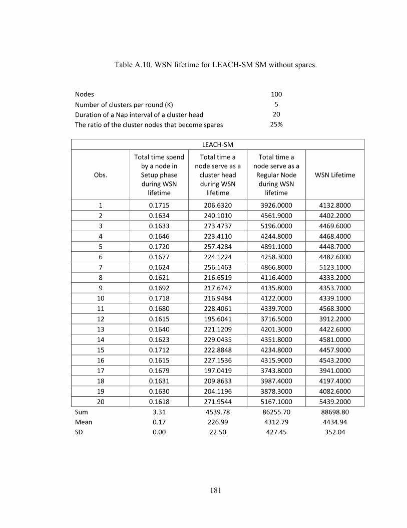
181
Table A.10. WSN lifetime for LEACH-SM SM without spares.
Nodes 100
Number of clusters per round (K) 5
Duration of a Nap interval of a cluster head 20
The ratio of the cluster nodes that become spares 25%
LEACH‐SM
Obs.
Total time spend by a node in Setup phase during WSN lifetime
Total time a node serve as a cluster head during WSN lifetime
Total time a node serve as a Regular Node during WSN lifetime
WSN Lifetime
1 0.1715 206.6320 3926.0000 4132.8000
2 0.1634 240.1010 4561.9000 4402.2000
3 0.1633 273.4737 5196.0000 4469.6000
4 0.1646 223.4110 4244.8000 4468.4000
5 0.1720 257.4284 4891.1000 4448.7000
6 0.1677 224.1224 4258.3000 4482.6000
7 0.1624 256.1463 4866.8000 5123.1000
8 0.1621 216.6519 4116.4000 4333.2000
9 0.1692 217.6747 4135.8000 4353.7000
10 0.1718 216.9484 4122.0000 4339.1000
11 0.1680 228.4061 4339.7000 4568.3000
12 0.1615 195.6041 3716.5000 3912.2000
13 0.1640 221.1209 4201.3000 4422.6000
14 0.1623 229.0435 4351.8000 4581.0000
15 0.1712 222.8848 4234.8000 4457.9000
16 0.1615 227.1536 4315.9000 4543.2000
17 0.1679 197.0419 3743.8000 3941.0000
18 0.1631 209.8633 3987.4000 4197.4000
19 0.1630 204.1196 3878.3000 4082.6000
20 0.1618 271.9544 5167.1000 5439.2000
Sum 3.31 4539.78 86255.70 88698.80
Mean 0.17 226.99 4312.79 4434.94
SD 0.00 22.50 427.45 352.04

182
Table A.11. WSN lifetime for LEACH.
Nodes 100
Number of clusters per round (K) 5
Duration of a Nap interval of a cluster head 20
The ratio of the cluster nodes that become spares 50%
LEACH
Obs.
Total time spend by a node in Setup phase during WSN lifetime
Total time a node serve as a cluster head during WSN lifetime
Total time a node serve as a Regular Node during WSN lifetime
WSN Lifetime
1 0.1631 175.2982 3330.7000 3406.1000
2 0.1699 177.5933 3374.3000 3582.0000
3 0.1686 170.7223 3243.7000 3424.6000
4 0.1713 166.1247 3156.4000 3624.7000
5 0.1623 177.6224 3374.8000 3553.6000
6 0.1655 168.4780 3201.1000 3369.7000
7 0.1620 171.1654 3252.1000 3423.5000
8 0.1635 186.1131 3536.1000 3722.4000
9 0.1633 184.8711 3512.6000 3697.6000
10 0.1664 177.4844 3372.2000 3579.9000
11 0.1668 174.6445 3318.2000 3493.1000
12 0.1681 178.0001 3382.0000 3560.2000
13 0.1639 167.8516 3189.2000 3357.2000
14 0.1672 170.3498 3236.6000 3507.2000
15 0.1639 163.2630 3102.0000 3265.4000
16 0.1633 172.5143 3277.8000 3450.5000
17 0.1703 160.3497 3046.6000 3307.2000
18 0.1695 158.7262 3015.8000 3674.7000
19 0.1617 169.6826 3224.0000 3393.8000
20 0.1674 164.9457 3134.0000 3799.1000
Sum 3.32 3435.80 65280.20 70192.50
Mean 0.17 171.79 3264.01 3509.63
SD 0.00 7.34 139.46 146.10

183
Table A.12. WSN lifetime for LEACH-SM SM without spares.
Nodes 100
Number of clusters per round (K) 5
Duration of a Nap interval of a cluster head 20
The ratio of the cluster nodes that become spares 50%
LEACH‐SM
Obs.
Total time spend by a node in Setup phase during WSN lifetime
Total time a node serve as a cluster head during WSN lifetime
Total time a node serve as a Regular Node during WSN lifetime
WSN Lifetime
1 0.1718 302.6009 5749.4000 6052.2000
2 0.1709 330.4699 6278.9000 6609.6000
3 0.1664 305.8475 5811.1000 6117.1000
4 0.1716 323.0541 6138.0000 6061.3000
5 0.1688 285.5032 5424.6000 6710.2000
6 0.1645 403.3928 7664.5000 6028.0000
7 0.1613 467.4327 8881.2000 6358.8000
8 0.1682 351.8020 6684.2000 6066.2000
9 0.1652 325.8142 6190.5000 6516.4000
10 0.1694 324.8554 6172.3000 6427.3000
11 0.1649 241.5679 4589.8000 4831.5000
12 0.1625 343.6164 6528.7000 6802.5000
13 0.1689 241.0694 4580.3000 4821.6000
14 0.1628 288.4456 5480.5000 6769.1000
15 0.1638 322.5155 6127.8000 6410.5000
16 0.1680 342.0339 6498.6000 6840.8000
17 0.1672 327.1116 6215.1000 6542.4000
18 0.1653 400.0921 7601.8000 6002.0000
19 0.1698 349.0465 6631.9000 5981.1000
20 0.1612 409.0173 7771.3000 6080.5000
Sum 3.33 6685.29 127020.50 124029.10
Mean 0.17 334.26 6351.03 6201.46
SD 0.00 54.85 1042.15 554.11

184
Table A.13. WSN lifetime for LEACH.
Nodes 100
Number of clusters per round (K) 5
Duration of a Nap interval of a cluster head 30
The ratio of the cluster nodes that become spares 25%
LEACH
Obs.
Total time spend by a node in Setup phase during WSN lifetime
Total time a node serve as a cluster head during WSN lifetime
Total time a node serve as a Regular Node during WSN lifetime
WSN Lifetime
1 0.1669 281.5616 5349.7000 5131.4000
2 0.1628 270.5420 5140.3000 4411.0000
3 0.1700 265.1251 5037.4000 5302.7000
4 0.1626 286.2647 5439.0000 4725.5000
5 0.1618 280.2025 5323.8000 4604.2000
6 0.1681 273.2505 5191.8000 4465.2000
7 0.1630 287.8976 5470.1000 4758.1000
8 0.1649 258.8184 4917.6000 5176.5000
9 0.1641 275.6754 5237.8000 5313.7000
10 0.1720 266.4354 5062.3000 4328.9000
11 0.1689 260.6762 4952.8000 5213.7000
12 0.1630 290.3519 5516.7000 4607.2000
13 0.1632 278.8141 5297.5000 4676.4000
14 0.1706 258.5251 4912.0000 4970.7000
15 0.1665 281.5127 5348.7000 4690.4000
16 0.1676 275.3527 5231.7000 4507.2000
17 0.1703 249.7055 4744.4000 4964.3000
18 0.1623 264.0593 5017.1000 5281.3000
19 0.1677 282.6763 5370.8000 5353.7000
20 0.1631 277.3083 5268.9000 4646.3000
Sum 3.32 5464.76 103830.40 97128.40
Mean 0.17 273.24 5191.52 4856.42
SD 0.00 11.12 211.32 338.33

185
Table A.14. WSN lifetime for LEACH-SM SM without spares.
Nodes 100
Number of clusters per round (K) 5
Duration of a Nap interval of a cluster head 30
The ratio of the cluster nodes that become spares 25%
LEACH‐SM
Obs.
Total time spend by a node in Setup phase during WSN lifetime
Total time a node serve as a cluster head during WSN lifetime
Total time a node serve as a Regular Node during WSN lifetime
WSN Lifetime
1 0.1702 261.6247 4970.9000 6232.7000
2 0.1669 268.5962 5103.3000 6372.1000
3 0.1659 337.0604 6404.1000 6741.4000
4 0.1655 262.1918 4981.6000 6144.0000
5 0.1670 285.9616 5433.3000 5719.4000
6 0.1659 270.7963 5145.1000 5416.1000
7 0.1652 315.4221 5993.0000 6108.6000
8 0.1713 283.0772 5378.5000 5691.7000
9 0.1672 290.6452 5522.3000 5813.1000
10 0.1689 285.3652 5421.9000 5757.5000
11 0.1631 270.6203 5141.8000 5412.6000
12 0.1673 268.8798 5108.7000 6370.8000
13 0.1662 319.9102 6078.3000 6378.4000
14 0.1653 323.0586 6138.1000 6461.3000
15 0.1677 322.2471 6122.7000 6445.1000
16 0.1643 326.2560 6198.9000 6525.3000
17 0.1692 291.8772 5545.7000 5837.7000
18 0.1709 305.5270 5805.0000 6110.7000
19 0.1658 352.0400 6688.8000 7041.0000
20 0.1622 307.0719 5834.4000 6141.6000
Sum 3.34 5948.23 113016.40 122721.10
Mean 0.17 297.41 5650.82 6136.06
SD 0.00 26.95 512.10 427.23

186
Table A.15. WSN lifetime for LEACH.
Nodes 100
Number of clusters per round (K) 5
Duration of a Nap interval of a cluster head 30
The ratio of the cluster nodes that become spares 50%
LEACH
Obs.
Total time spend by a node in Setup phase during WSN lifetime
Total time a node serve as a cluster head during WSN lifetime
Total time a node serve as a Regular Node during WSN lifetime
WSN Lifetime
1 0.1689 226.7033 4307.4000 4834.2000
2 0.1670 228.9510 4350.1000 4879.2000
3 0.1719 224.8302 4271.8000 4996.8000
4 0.1698 230.0951 4371.8000 4602.1000
5 0.1642 237.5064 4512.6000 4950.3000
6 0.1669 223.1495 4239.8000 4963.2000
7 0.1686 234.7018 4459.3000 4994.2000
8 0.1639 242.8927 4615.0000 4828.0000
9 0.1698 224.6986 4269.3000 4994.1000
10 0.1713 237.4760 4512.0000 4949.7000
11 0.1697 232.4643 4416.8000 4649.5000
12 0.1631 232.9300 4425.7000 4658.8000
13 0.1679 238.0126 4522.2000 4960.4000
14 0.1641 230.5810 4381.0000 4911.8000
15 0.1675 227.6449 4325.3000 4853.1000
16 0.1683 226.6526 4306.4000 4933.2000
17 0.1690 235.3701 4472.0000 4907.6000
18 0.1662 229.8926 4368.0000 4598.0000
19 0.1657 226.7539 4308.3000 4935.2000
20 0.1676 230.6013 4381.4000 4912.2000
Sum 3.35 4621.91 87816.20 97311.60
Mean 0.17 231.10 4390.81 4865.58
SD 0.00 5.26 99.96 132.14

187
Table A.16. WSN lifetime for LEACH-SM SM without spares.
Nodes 100
Number of clusters per round (K) 5
Duration of a Nap interval of a cluster head 30
The ratio of the cluster nodes that become spares 50%
LEACH‐SM
Obs.
Total time spend by a node in Setup phase during WSN lifetime
Total time a node serve as a cluster head during WSN lifetime
Total time a node serve as a Regular Node during WSN lifetime
WSN Lifetime
1 0.1615 537.2395 10208.0000 8045.0000
2 0.1656 374.1804 7109.4000 8453.8000
3 0.1647 445.5092 8464.7000 8990.3000
4 0.1621 567.6947 10786.0000 8354.0000
5 0.1670 366.8501 6970.2000 8337.2000
6 0.1682 451.2500 8573.7000 9025.2000
7 0.1686 523.4394 9945.3000 8469.0000
8 0.1685 435.8401 8281.0000 8717.0000
9 0.1612 466.0726 8855.4000 8321.6000
10 0.1662 449.6604 8543.5000 8993.4000
11 0.1698 557.5700 10594.0000 8552.0000
12 0.1664 506.0552 9615.0000 8117.0000
13 0.1693 366.9614 6972.3000 8339.0000
14 0.1632 584.5119 11106.0000 8589.0000
15 0.1672 408.2603 7756.9000 8165.4000
16 0.1682 460.0585 8741.1000 9201.3000
17 0.1624 447.4633 8501.8000 8949.4000
18 0.1697 403.8459 7673.1000 8077.1000
19 0.1704 418.3749 7949.1000 8367.7000
20 0.1708 487.6586 9265.5000 9553.3000
Sum 3.33 9258.50 175912.00 171617.70
Mean 0.17 462.92 8795.60 8580.89
SD 0.00 66.00 1254.00 414.25

188
Table A.17. WSN lifetime for LEACH-SM with spares.
Nodes 100
Number of clusters per round (K) 5
Duration of a Nap interval of a cluster head 0
The ratio of the cluster nodes that become spares 25%
LEACH‐SM First Replacement
Obs. Number of Frames per Round
WSN Lifetime Lifetime of Spares
Number of Frames per Round
WSN Lifetime
1 28820 1014.1000 6928.0
2 28459 1001.4000 6924.9
3 36238 1075.1000 7146.1
4 30638 998.1000 6982.2
5 35516 949.7000 7118.3
6 26819 973.6927 6875.4
7 32708 958.9000 7047.5
8 31628 913.9000 7012.2
9 36176 1072.9000 7136.8
10 30725 1081.1000 6989.8
11 30795 1083.6000 6992.1
12 33319 1172.4000 7062.7
13 27937 983.0288 6903.5
14 37835 1331.2000 7189.8
15 29299 1030.9000 6945.5
16 28738 911.2000 6931.3
17 25720 905.0294 6843.7
18 33499 1178.7000 7067.6
19 31551 1010.2000 7013.7
20 27492 967.3681 6895.9
Sum 623912.00 20612.52 140007.00 Mean 31195.60 1030.63 7000.35 SD 3420.73 104.87 97.41
Note: No replacement possible in this case.

189
Table A.18. WSN lifetime for LEACH-SM with spares.
Nodes 100
Number of clusters per round (K) 5
Duration of a Nap interval of a cluster head 0
The ratio of the cluster nodes that become spares 50%
LEACH‐SM First Replacement
Obs. Number of Frames per Round
WSN Lifetime Lifetime of Spares
Number of Frames per Round
WSN Lifetime
1 36649 1172.5000 6502.1 31675 2685.8000
2 41322 1321.9000 6620.1 35176 2547.3000
3 35729 1143.0000 6479.3 30990 2634.5000
4 55997 1791.3000 7001 46263 3271.3000
5 40914 1308.9000 6608.6 34807 2422.4000
6 39228 1254.9000 6568.3 33685 2632.6000
7 40646 1300.3000 6605.5 34822 2514.3000
8 55005 1759.6000 6968.7 44941 3197.3000
9 50287 1608.7000 6856.4 42293 2961.7000
10 38804 1441.4000 6559.3 33453 2311.6000
11 33569 1473.9000 6423.6 29263 2010.1000
12 54237 1705.0000 6949.2 44430 3156.4000
13 44956 1458.2000 6714.4 37979 2653.2000
14 40444 1293.8000 6600.5 34675 2403.1000
15 37477 1198.9000 6525.9 32447 2237.0000
16 53617 1735.2000 6937.7 44377 3134.8000
17 58353 1896.7000 7058.2 47610 3389.8000
18 45495 1485.4000 6727.6 38341 2682.0000
19 38691 1257.8000 6554.1 33246 2301.4000
20 38017 1226.2000 6539.7 32868 2267.7000
Sum 879437.00 28833.60 133800.20 743341.00 53414.30
Mean 43971.85 1441.68 6690.01 37167.05 2670.72
SD 7743.02 232.44 198.07 5709.47 392.01
Note: No replacement possible in this case.

190
Table A.19. WSN lifetime for LEACH-SM with spares.
Nodes 100
Number of clusters per round (K) 5
Duration of a Nap interval of a cluster head 10
The ratio of the cluster nodes that become spares 25%
LEACH‐SM First Replacement
Obs. Number of Frames per Round
WSN Lifetime Lifetime of Spares
Number of Frames per Round
WSN Lifetime
1 33247 2944.7000 17779
2 28902 2539.9000 17464
3 30453 2667.3000 17570
4 27410 2417.8000 17345
5 34097 3020.0000 17820
6 30156 2651.0000 17539
7 27241 2712.8000 17336
8 27668 2450.6000 17364
9 25995 2702.4000 17239
10 35880 3177.9000 17950
11 26847 2577.9000 17315
12 30363 2659.3000 17554
13 38375 3368.9000 18140
14 34059 3016.6000 17819
15 38499 3409.9000 18138
16 25749 2280.6000 17226
17 26905 2383.0000 17312
18 33764 2990.5000 17793
19 25113 2224.3000 17180
20 27666 2450.4000 17370
Sum 608389.00 54645.80 351253.00 Mean 30419.45 2732.29 17562.65 SD 4203.31 344.77 300.93
Note: No replacement possible in this case.

191
Table A.20. WSN lifetime for LEACH-SM with spares.
Nodes 100
Number of clusters per round (K) 5
Duration of a Nap interval of a cluster head 10
The ratio of the cluster nodes that become spares 50%
LEACH‐SM First Replacement
Obs. Number of Frames per Round
WSN Lifetime Lifetime of Spares
Number of Frames per Round
WSN Lifetime
1 38633 3829.7000 17660 33296 6199.4000
2 38534 3821.1000 17644 33045 6169.2000
3 53038 3871.1000 18659 44181 7378.9000
4 37136 3200.6000 17553 32072 6404.9000
5 34163 2974.4000 17341 29622 5597.5000
6 38152 3288.2000 17624 32883 6492.3000
7 39725 3423.8000 17747 34379 6696.8000
8 46796 4033.2000 18223 39478 7435.7000
9 54082 3861.1000 18723 44679 8411.8000
10 56652 4782.6000 18899 46416 7083.0000
11 56651 4782.5000 18902 46527 7052.5000
12 55911 4718.7000 18858 46252 7805.0000
13 48261 4159.4000 18335 40847 7679.9000
14 41302 3559.7000 17843 35325 6604.3000
15 53267 3890.9000 18668 44117 8150.1000
16 34291 2955.5000 17360 29894 6502.0000
17 44372 3824.3000 18061 37803 7002.4000
18 50618 3862.6000 18482 42149 7995.2000
19 57034 3815.5000 18917 46372 7902.1000
20 43836 3778.1000 18027 37472 7007.7000
Sum 922454.00 76433.00 363526.00 776809.00 141570.70
Mean 46122.70 3821.65 18176.30 38840.45 7078.54
SD 8070.38 522.54 557.02 5981.64 755.92
Note: No replacement possible in this case.

192
Table A.21. WSN lifetime for LEACH-SM with spares.
Nodes 100
Number of clusters per round (K) 5
Duration of a Nap interval of a cluster head 20
The ratio of the cluster nodes that become spares 25%
LEACH‐SM First Replacement
Obs. Number of Frames per Round
WSN Lifetime Lifetime of Spares
Number of Frames per Round
WSN Lifetime
1 25641 4170.9000 27076
2 34941 4066.0000 28141
3 26368 3872.1000 27156
4 37114 5168.6000 28379
5 29179 4063.6000 27497
6 28244 4933.4000 27376
7 30818 4291.8000 27659
8 36155 5035.0000 28263
9 36246 5047.7000 28285
10 28352 3948.4000 27393
11 29857 4158.0000 27539
12 30834 4294.1000 27673
13 31553 4394.2000 27763
14 36952 5146.0000 28359
15 25744 3585.2000 27114
16 35897 4999.1000 28227
17 35649 4964.6000 28209
18 31236 4350.0000 27730
19 30110 4193.2000 27576
20 28766 4006.1000 27434
Sum 629656.00 88688.00 554849.00 Mean 31482.80 4434.40 27742.45 SD 3883.84 492.80 437.59
Note: No replacement possible in this case.

193
Table A.22. WSN lifetime for LEACH-SM with spares.
Nodes 100
Number of clusters per round (K) 5
Duration of a Nap interval of a cluster head 20
The ratio of the cluster nodes that become spares 50%
LEACH‐SM First Replacement
Obs. Number of Frames per Round
WSN Lifetime Lifetime of Spares
Number of Frames per Round
WSN Lifetime
1 48185 6809.0000 30027 40358 10512.0000
2 50520 6139.0000 30293 42090 11087.0000
3 39887 5636.5000 29078 34035 10446.0000
4 48139 6802.5000 30032 40498 11525.0000
5 36883 5212.0000 28756 31929 10723.9000
6 43497 6146.6000 29492 36833 11351.0000
7 45026 6362.6000 29664 37958 11726.0000
8 38051 5377.0000 28870 32626 9987.4000
9 48858 6904.1000 30105 40893 12683.0000
10 50475 6132.6000 30302 42295 10109.0000
11 51747 6312.3000 30423 42794 11360.0000
12 47640 6732.0000 29987 40306 12828.0000
13 41686 5890.7000 29308 35742 11141.0000
14 33343 6011.7000 28370 29258 11846.2000
15 53129 6007.6000 30596 44097 11739.0000
16 47992 6781.7000 30017 40408 12492.0000
17 47335 6358.9000 29934 39795 12312.0000
18 50334 6012.7000 30294 42322 13093.0000
19 54212 6050.7000 30719 44876 11002.0000
20 53182 6350.1000 30609 44272 11771.0000
Sum 930121.00 124030.30 596876.00 783385.00 229734.50
Mean 46506.05 6201.52 29843.80 39169.25 11486.73
SD 5860.86 467.10 664.77 4425.62 892.78
Note: No replacement possible in this case.

194
Table A.23. WSN lifetime for LEACH-SM with spares.
Nodes 100
Number of clusters per round (K) 5
Duration of a Nap interval of a cluster head 30
The ratio of the cluster nodes that become spares 25%
LEACH‐SM First Replacement
Obs. Number of Frames per Round
WSN Lifetime Lifetime of Spares
Number of Frames per Round
WSN Lifetime
1 29371 6023.7000 40489
2 26870 5510.7000 40109
3 33674 6906.1000 41206
4 28386 5821.6000 40342
5 26650 5465.6000 40063
6 26393 5412.9000 40043
7 34756 7128.0000 41369
8 34683 6113.1000 41385
9 30029 6158.6000 40598
10 27544 5649.0000 40204
11 30074 6167.8000 40594
12 38078 7809.3000 41920
13 30342 6222.8000 40648
14 28208 6360.1000 40288
15 28023 5747.2000 40260
16 28317 5807.5000 40350
17 35920 6166.7000 41607
18 28848 5916.4000 40388
19 30423 6239.4000 40678
20 33139 6096.4000 41150
Sum 609728.00 122722.90 813691.00 Mean 30486.40 6136.15 40684.55 SD 3388.17 583.51 557.01
Note: No replacement possible in this case.

195
Table A.24. WSN lifetime for LEACH-SM with spares.
Nodes 100
Number of clusters per round (K) 5
Duration of a Nap interval of a cluster head 30
The ratio of the cluster nodes that become spares 50%
LEACH‐SM First Replacement
Obs. Number of Frames per Round
WSN Lifetime Lifetime of Spares
Number of Frames per Round
WSN Lifetime
1 35885 7027.8000 39679 31006 13100.0000
2 42255 8275.3000 40716 36263 15377.0000
3 35234 8470.3000 39568 30426 12859.0000
4 37347 7314.1000 39930 32317 15643.0000
5 57112 11185.0000 43048 47197 20428.0000
6 35638 6979.4000 39666 31003 14510.0000
7 44314 8678.5000 41044 37880 16097.0000
8 39448 7725.5000 40261 33967 14378.0000
9 58262 11410.0000 43216 47817 20775.0000
10 55708 10910.0000 42775 45433 19807.0000
11 45918 8992.6000 41277 38899 16611.0000
12 33546 6569.7000 39341 29361 12320.0000
13 47606 9323.2000 41560 40356 17227.0000
14 35011 6856.6000 39565 30493 12828.0000
15 43640 8546.5000 40918 37165 15825.0000
16 40267 7885.9000 40373 34448 14632.0000
17 48639 9525.5000 41684 40680 17492.0000
18 47490 9300.5000 41538 40221 17177.0000
19 36771 7201.3000 39864 32053 13479.0000
20 48163 9432.3000 41612 40355 17335.0000
Sum 868254.00 171610.00 817635.00 737340.00 317900.00
Mean 43412.70 8580.50 40881.75 36867.00 15895.00
SD 7644.67 1449.13 1199.75 5717.26 2507.53
Note: No replacement possible in this case.

196
BIBLIOGRAPHY
[ACSS06] A. Gallais, J. Carle, D. Simplot-Ryl and I. Stojmenovic, “Ensuring Area k-
Coverage in Wireless Sensor Networks with Realistic Physical Layers,”
IEEE Conf. on Digital Object Identifier, 2006, pp. 880 – 883.
[AlGa08] C. Alippi and C. Galperti, “An Adaptive System for Optimal Solar Energy
Harvesting in Wireless Sensor Network Nodes,” IEEE Trans. on Circuits
and Systems I: Regular Papers, vol. 55(6), 2008, pp. 1742 – 1750.
[AlGa08] C. Alippi and C. Galperti, “An Adaptive System for Optimal Solar Energy
Harvesting in Wireless Sensor Network Nodes,” IEEE Trans. on Circuits
and Systems I: Regular Papers, vol. 55(6), 2008, pp. 1742 – 1750.
[ASSC02] I. F. Akyildiz and W. Su, Y. Sankarasubramaniam and E. Cayirci,
“Wireless sensor networks: A survey,” Elsevier Computer Networks, vol.
38(4), 2002, pp. 393 – 422.
[BaLi11] B. Abu Bakr and L. Lilien, “A Quantitative Comparison of Energy
Consumption and WSN Lifetime for LEACH and LEACH-SM,” Proc.
Fourth Intl. Workshop on Sensor Networks (SN 2011), in conjunction with
ICDCS 2011, Minneapolis, MN, June 2011 (to appear).
[BaLi11] B. Abu Bakr and L. Lilien, “Extending Wireless Sensor Network Lifetime
in the LEACH-SM Protocol by Spare Selection,” Proc. First Intl.

197
Workshop on Advanced Communication Technologies and Applications to
Intelligent Transportation Systems, Cognitive Radios and Sensor Networks
(ACTICS), Busan, Korea, June 2011 (to appear).
[BaLi11] B. Abu Bakr and L. Lilien, “LEACH-SM: A Protocol for Extending
Wireless Sensor Network Lifetime by Management of Spare Nodes,”
Proc. 3S Workshop (Wireless of the Student, by the Student, for the
Student) in conjunction with WiOpt 2011, Princeton, NJ, May 2011 (to
appear).
[ChHa10] Z. Changlun and M.Haibing, “An Efficiency Measure Approach for
Wireless Sensor Networks,” Proc. IEEE Intl. Conf. on Information
Technology and Applications (IFITA), vol. 3, 2010, pp. 49 – 52.
[ChPi907] A. Chamam and S. Pierre, “Energy-Efficient State Scheduling for
Maximizing Sensor Network Lifetime under Coverage Constraint,”
Wireless and Mobile Computing, Networking and Communications, 2007,
pp. 63 – 63.
[DJPF09] W. Di, L. Jun, X. Peng, Q. Fei, L. Ling, W. Wei, and L. Xuehui “Study on
How to Deal with Experimental Data of Physics Based on MATLAB Web
Server,” Proc. IEEE Intl. Conf. on Computer Science-Technology and
Applications, vol. 3, 2009, pp. 274 – 277.

198
[Dress07] F. Dressler, Self-Organization in Sensor and Actor Networks. Wiley Series
in Communications Networking & Distributed Systems, 2007.
[DVC06] S. Dasika, S. Vrudhhula and K. Chopra, “Algorithms for Maximizing
Lifetime of Battery-Powered Wireless Sensor Nodes,” Sensor Network
Operations, John Wiley & Sons, 2006, pp. 367–397.
[DVCR04] S. Dasika, S. Vrudhula, K. Chopra and S. Ramasubramanian, “A
Framework for Battery-Aware Sensor Management,” Proc. Conf. on
Design, Automation and Test in Europe, vol. 2, 2004, pp. 962- 967.
[EsPe08] M. Esseghir and H. Perros, “Optimizing the wireless sensor network
lifetime under reliability constraint,” Proc. IEEE Intl. Conf. on Wireless
Days (IFIP), 2008, pp. 1 – 5.
[EuKw11] P. Eunil and C. Kwangsu, “Performance Evaluation of Energy Efficient
and Reliable Geographic Routing in WSNs,” Proc. IEEE Intl. Conf. on
Information Science and Applications (ICISA), 2011, 1 – 8.
[GDPV03] S.R. Gandham, M. Dawande, R. Prakash and S. Venkatesan, “Energy
efficient schemes for wireless sensor networks with multiple mobile base
stations,” Proc. IEEE Intl. Conf. on Global Telecommunications
Conference (GLOBECOM), vol. 1, December 2003, pp. 377 – 381.
[GSS09] S. Gupta, M.Sharma and S. Sharma, “Simulation for Energy Expenditure
Estimation of WSN for Comparison of Network Routing Protocols.” Proc.

199
IEEE Intl. Conf. on Emerging Trends in Engineering and Technology
(ICETET), 2009, pp. 1115 - 1118.
[Hein00] W. B. Heinzelman, “Application-Specific Protocol Architectures for
Wireless Networks.” Ph.D. Dissertation, Department of Electrical
Engineering and Computer Science, MIT, Cambridge, MA, June 2000.
[HKTM09] M. Hasegawa, T. Kawamura, H. N. Tran, G. Miyamoto, Y. Murata, H.
Harada and S. Kato, “Decentralized optimization of wireless sensor
network lifetime based on neural network dynamics,” Proc. IEEE Intl.
Conf. on Personal, Indoor and Mobile Radio Communications (PIMRC),
2008, p. 1.
[HoCa10] L. Hong and J. Cai, “The application guide of mixed programming
between MATLAB and other programming languages,” Proc. IEEE Intl.
Conf. on Computer and Automation Engineering (ICCAE), vol. 3, 2010,
pp. 185 – 189.
[IAM10] A. Ibrahem, A. Akram and M. Mahmood, “Simulation & performance
study of wireless sensor network (WSN) using MATLAB,” Proc. IEEE
Intl. Conf. on Energy, Power and Control (EPC-IQ), 2010, pp. 307 – 314.
[JBS07] D. Jung, T. Teixeira, A. Barton-Sweeney and A. Savvides, “Model-Based
Design Exploration of Wireless Sensor Node Lifetimes,” Proc. 4th
European Conf. on Wireless Sensor Networks, 2007, pp. 277-292.

200
[JiZh06] Z. Jiang and M. Zhou, “A Dynamic-Bandwidth-Allocation-with-Collision-
Avoidance MAC Design for Mobile Ad Hoc Network,” Proc. IEEE Intl.
Conf. on Networking, Sensing and Control (ICNSC), August 2006 , pp.
18-24.
[LWYW06] B. Li, Q. Wang, Y. Yang and J. Wang, “Optimal Distribution of
Redundant Sensor Nodes for Wireless Sensor Networks,” Proc. IEEE Intl.
Conf. on Industrial Informatics, 2006, pp. 985 – 989.
[MaSe09] N. H. Mak and W. K. G. Seah, “How Long is the Lifetime of a Wireless
Sensor Network?,” Proc. IEEE Intl. Conf. on Advanced Information
Networking and Applications (AINA), 2009, p. 763.
[MWHA09] V. Merrett, M. White, R. Harris and M. Al-Hashimi, “Energy-Aware
Simulation for Wireless Sensor Networks,” Proc. IEEE Intl. Conf. on
Sensor, Mesh and Ad Hoc Communications and Networks, 2009, pp. 1 - 8
[PrGa10] A. Prajapati and S. Ganesan, “S-CAS: Smart channel assignment scheme
for wireless sensor networks,” Proc. IEEE Intl. Conf. on
Electro/Information Technology (EIT), October 2010, pp. 1-6
[RGM08] L. Ren, Z. Guo and R. Ma, “Prolonging Sensor Network Lifetime with
Initial Energy Level Assignment,” Software Engineering, Artificial
Intelligence, Networking, and Parallel/Distributed Computing, 2008, pp.
231 – 236.

201
[SLZ08] W. Song, Y. Liu and S. Zhang, “Research on SMAC Protocol for WSN
Wireless Communications,” Proc. 4th Intl. Conf. on Networking and
Mobile Computing (WiCOM), 2008, pp.1 – 4.
[SuSh10] F. Sun and M. Shayman, “Prolonging Network Lifetime via Partially
Controlled Node Deployment and Adaptive Data Propagation in WSN,”
Proc. IEEE Intl. Conf. on Information Sciences and Systems (CISS), vol.
1, March 2010, pp. 226 – 231.
[Tin02] TinyOs, Feb. 2002. Available online at: http://www.tinyos.net/
[VDMC08] R. Verdone, D. Dardari, G. Mazzini and A. Conti, Wireless Sensor and
Actuator Networks Technologies, Analysis and Design, London:
Academic Press, 2008.
[XLY09] S. Xiong, J. Li and L. Yu, “Maximize the Lifetime of a Data-gathering
Wireless Sensor Network,” Proc. IEEE Intl. Conf. on Sensor, Mesh and
Ad Hoc Communications and Networks (SECON), 2009, p. 1.
[XSH08] X. Xian, W. Shi and H. Huang, “Comparison of OMNET++ and other
simulators for WSN simulation,” Proc. IEEE Intl. Conf. on Industrial
Electronics and Applications(ICIEA), 2008, pp. 1439 – 1443.
[YHE02] W. Ye, J. Heidemann and D. Estrin, “An energy-efficient MAC protocol
for wireless sensor networks,” Proc. IEEE Intl. Conf. on Computer and

202
Communications Societies (INFOCOM), vol. 3, November 2002, pp.
1567-1572.
[YHE04] W. Ye, J. Heidemann and D. Estrin, “Medium access control with
coordinated adaptive sleeping for wireless sensor networks,” IEEE/ACM
Trans. on Networking, vol. 12(3), 2004, pp. 493 – 506.
[ZDLC09] X. Zhang, X. Ding, S. Lu and G. Chen, “Principles for Energy-Efficient
Topology Control in Wireless Sensor Networks,” Proc. IEEE Intl. Conf.
on Wireless Communications, Networking and Mobile Computing
(WiCom), October 2009, pp. 1-6.
[ZLX08] J. Zhang, D. Liu and Y. Xu, “An Efficient Power and Coverage Algorithm
in WSNs,” Proc. of the Intl. Multisymposiums on Computer and
Computational Sciences, 2008, pp. 102-105.
[ZXWP06] Z. Zhou, X. Xang, X. Wang and J. Pan, “An energy-efficient data-
dissemination protocol in wireless sensor networks,” World of Wireless,
Mobile and Multimedia Networks, 2006, pp. 10 – 22.
[ZZLY10] H. Zhang, M. Zheng, J. Li, H. Yu and P. Zeng, “Redundancy control for
reliability-lifetime tradeoff in energy harvesting wireless sensor
networks,” Proc. IEEE Intl. Conf. on Computer Design and Applications
(ICCDA), vol. 2, 2010, pp. 544 – 548.