lay-flat irrigation tubing

y- '2-

Hydraulic and Geometrical

Relationships of

LAY-FLAT IRRIGATION TUBING

V0BR

Technical Bulletin No. 1309

Agricultural Research Service U.S. DEPARTMENT OF AGRICULTURE In Cooperation With UTAH AGRICULTURAL EXPERIMENT STATION

CONTENTS

PBOBIíEM- .-^ ^^-.-- -- 2

HEAD LOSB IN FLOW CONI>üI1"S 3 Pîpe-___ . 3 Parallel Boundaries.--^-.^ 4 Lay-Flat Tubing 4

HYDROSTATIC TESTS 5 Experimental Tests.«. 6 Data Analysis and Presentation 8 Discussion of Results« 18

FLOW TESTS 20 Experimental Procedure 20 Data Analysis and Presentation 22 Discussion ^ 27 Discharge Diagrams 31

SUMMARY 37 Static Tests 37 Flow Tests 37

SYMBOLS AND DEFINITIONS 38

Washington, D.C. Issued October 1964

For sale by the Superintendent of Documents, U.S. Government Printing OflBce Washington, D.C., 20402 Price 20 cents

Hydraulic and Geometrical Relationships of LAY-FLAT

IRRIGATION TUBING ' By ALLAN S. HUMPHERYS, agricultural engineerJ and C. W. LAURITZEN, soil

scientist, Soil and Water Conservation Research Division, Agricultural Research Service ^

Lay-flat tubing lies flat when empty like a deflated innertube section. The tubing is usually made from such materials as butyl rubber or plastic in which a supporting fabric is often built into the walls to impart additional strength.

It is often feasible in irrigation practice to replace farm ditches and laterals with lay-flat tubing, particularly in areas where seepage and erosion are problems. In addition, lay-flat tubing may be used for water distribution, as a temporary water conveyance, or as a conveyance where a ditch would be undesirable or impractical. Use of lay- flat tubing for irrigation is a relatively recent development. Conse- quently, information is not available to guide fabrication or to design properly a water distribution system hydraulically where it is used.

The investigation was undertaken to obtain information that would be useful in the hydraulic design of a water distribution system where lay-flat tubing is used. The principal objectives were (1) to obtain data from static head measurements from which the tube pressure- area-shape relationships coidd be determined; and (2) to determine a shape factor that would express the effect of cross-sectional shape upon the frictional head loss and allow conventional pipe design formulas to be modified and used for lay-flat tubing.

1 The experimental study summarizes a master's thesis by Allan S. Humpherys, which is on file in the Engineering Library, Utah State University, Logan, and entitled, ''An Experimental Study of the Pressure-Area-Shape Relationships of Lay-Flat Tubing and Their Effect Upon the HydrauHc Friction Factor/." The testing and laboratory phase of the study was undertaken cooperatively with the U.S. Department of Agriculture and the Utah Agricultural Experiment Station.

2 The authors express appreciation to the Union Carbide Plastics Co., Division of Union Carbide Corp., for financial support given to the investigation and for the experimental tubing used in both the static and flow tests; to Bono Products, Inc., for butyl rubber tubing furn:'shed for the static tests; to Vaughn E. Hansen, director, Utah Engineering Experiment Station, for his helpful suggestions and technical assistance; and to Richard Miles for assistance in the collection of data from the flow tests.

2 TECHNICAL BULLETIN 1309, U.S. DEPT. AGRICULTURE

I FIGURE 1.—Definition sketch showing lay-flat tubing geometry.

PROBLEM The shape or degree of roundness and the cross-sectional area of a

tube are dependent primarily upon the fluid pressure inside (fig. 1). Above a certain pressure, the tubing approaches a circular cross section. When circular, the tube may be designed hydraulicaJly by conventional pipe design methods. When the pressure inside the tube is reduced, the cross-sectional area becomes smaller and approaches an oval-to-rectangular shape. This change in shape and area results in a nonuniform velocity distribution in which the velocity pattern is different in the vertical direction from that in the horizontal. For a given flow, this change in tube cross section is accompanied by a corresponding change in the mean fluid velocity. The head loss, therefore, is affected, since it is a function of both the velocity distribution and the mean velocity.

Most friction loss in a pipe or tube is dissipated near the boundary because of boundary drag. When the area and degree of roundness for a given tube are decreased, the boundary area becomes larger in proportion to the cross-sectional area. The energy loss, therefore, is affected by any change in tubing geometry that affects the ratio of the cross-sectional area to the perimeter or hydraulic radius.

Not all tubing is hydraulically smooth. Thin tubing constructed with a supporting fabric in its wall may be hydraulically rough. The relative roughness of this tubing is affected by a change in tube shape. Relative roughness is dej&ned as the ratio of the height of the boundary roughness projections e to the depth of flow midway between boundaries. It is usually expressed in terms of the pipe diameter and the plate spacing for pipe and parallel-boundary flow. A decrease in the degree of tubing roimdness results in a greater relative roughness value for a given tube, because the effective depth of flow between boundaries is decreased. Since the friction coefficient is related to both the relative roughness and velocity distribution, any shape change that affects either of these parameters will affect the head loss.

In most cases, the pressure along the length of the tube changes because of friction loss and elevation changes. As a result, the tube geometry and, hence, the fluid velocity are constantly changing from one section to another along the length of the tube. The flow, in this case, is nonuniform and the head loss due to friction in a given length of tubing is diflicult to determine.

LAY-FLAT IRRIGATION TUBING 3

HEAD LOSS IN FLOW CONDUITS

PIPE

Because of the similarity between lay-flat tubing and rigid pipe when used as closed conduits for fluid flow, the hydraulic design of tubing should be similar to that of a pipe.

Head loss for flow through a pipe is often expressed in the form ^

hr=K^ (1)

in which the value of n for laminar flow is unity, whereas for turbulent flow it ranges from 1.7 for smooth pipe to 2.0 for rough pipe.* The value of m for laminar flow is 2.0, whereas for turbulent flow its value ranges from 1.0 to approximately 1.3.

Dimensional analysis yields the following expression for pipe friction loss:

Ä,=2ÄR-|g (2)

or

in which the friction coeflicient / is a function of Reynolds number and relative roughness. Equation 3 is the basic expression for head loss through a pipe, and is known as the Darcy-Weisbach equation. Expressions for the coefficient / have been derived from the velocity- distribution equations by Karman and Prandtl.^ The Karman- Prandtl equation for/ in terms of Reynolds number for smooth-pipe flow is

^=21ogioR^(7-0.8. (4)

The companion equation for the rough-pipe coefficient is

^=2logio^+1.74. (5)

These equations are valid for the limiting boundary conditions of smooth and rough flow only. The coefficient for flow in the transition region between smooth and rough boundaries for commercial pipe is represented by the semiempiricalColebrook-White equation

3 RussEL, G. E. HYDRAULICS. Ed. 5. Pp. 181-183, illus. New York. 1947. ^ Symbols and definitions of terms used in this publication are given on p. 38. ^ ROUSE, HUNTER, ELEMENTARY MECHANICS OF FLUIDS. 376 pp., illus. New

York and London. 1946.


PARALLEL BOUNDARIES

The flow regime for uniform flow through lay-flat tubing ranges from that for rigid pipe to that for flow through parallel-boundary conduits. Rigid pipe and parallel boundaries represent the extreme conduit shapes. Therefore, expressions for the friction coefficients for flow through parallel boundaries, corresponding to those for pipe flow, are presented. The Karman-Prandtl equation for the resistance factor for smooth parallel boundaries of infinite extent is

^=2.03logioRV7-0.47. (7)

The equation for the parallel rough-boundary coefficient is

^=2.03 logio ^+2.11. (8)

Because of insufficient data, the constants in equations 7 and 8 have not been adjusted to provide agreement with experimental measurements.

The equations for pipe and parallel-boundary fiow are identical except for the integration constant. The factor 2.03 was adjusted to 2 in the pipe equations, to provide better agreement with experimental measurements. Since this factor appears in the expressions for both cross sections, the effect of conduit shape upon the friction factor must be represented by the integration constant for each type of flow.

The Darcy-Weisbach equation for parallel-boundary flow is

The diameter in equation 3 and twice the boundary spacing in equation 9 are each equal to four times the hydraulic radius for their respective cross-sectional shapes. Therefore, if the diameter and twice the boundary spacing are replaced by four times the hydraulic radius, the Darcy-Weisbach equation becomes

for both pipe and parallel-boundary flow.

LAY-FLAT TUBING

Keulegan ^ proposed equations for the friction coefficient for open channels of various cross sections in which the channel shape was

^ KEULEGAN, G. H. LAWS OF TURBULENT FLOW IN OPEN CHANNELS. [U.S.] Nati. Bur. Standards Jour. Res. 21: 707-741. (Res. Paper 1151.) 1938.


represented by a shape factor term in the expression. To the authors' knowledge, however, no equations have been developed for closed conduit flow covering the entire shape range between round and rectangular.

Since the general head-loss equation, equation 10, is the same for both pipe and parallel-boundary flow and since the expressions for / are the same at each end of the flow regime except for the constants embodying the shape effect, the friction loss through tubing may also be represented by this equation, inasmuch as lay-flat tubing represents a conduit that varies in shape from round to rectangular. It is necessary, however, to modify the friction coefficient to include the effects of shape change. When equation 10 is used for lay-flat tubing, /may be considered as consisting of two parts: (1) /', the friction coefficient for an equivalent flow through a pipe of the same diameter, and (2) a shape factor ß, which corrects/' for the effects of tube shape. In other words

J=ßf^ (11)

Thus, the frictional head loss for uniform flow through lay-flat tubing may be represented by

in which ß and R are the shape factor and hydraulic radius, respectively, for a given cross-sectional shape. The friction coefficient /'may be obtained from a conventional pipe resistance diagram of/ versus Keynolds number. The shape factor ß represents the ratio ///' and is evaluated empirically from flow test data obtained in this study.

HYDROSTATIC TESTS

As pointed out by Hansen,^ a study of the hydraulic properties of lay-flat tubing must be preceded by a study of the tube cross-sectional shape and area. Since the head loss and flow capacity of a conduit are a function of the conduit geometry, it is necessary, in studying tubing hydraulics, that its geometry at all pressure heads be known. It is also necessary to know the pressure head and velocity at a given location.

It would be difficult and generally impractical, because of the nature of the material, to install instruments to measure the flow velocity. If the cross-sectiona] area were known, the mean flow velocity could easily be determined from the continuity equation Q=aV at any point along the tube. As further indicated by Hansen, it may not be practical in some cases to attach pressure gages or taps to determine the piezometric pressure head at a location. The tubing geometry might be utilized for these purposes if data were available that related the tube geometry to the pressure head and cross-sectional area. These relationships were determined from hydrostatic tests made in the laboratory as herein described. The data are plotted in

7 HANSEN, V. E. FLEXIBLE PIPE FOB IRRIGATION WATER UNDER LOW PRESSURE.

Agr. Engin. 35(1): 32-33, 39. 1954.


dimensionless ratios and are, therefore, applicable to tubes of different diameters.

EXPERIMENTAL TESTS

Tubing Material Tested

Hydrostatic tests were made on tubes of different materials and sizes (table 1) in which the tube cross section was traced at different hydrostatic pressures. Two types of tubing were used: (1) a thin- walled vinyl chloride plastic and (2) a comparatively thick-walled butyl rubber tube. À 3-inch-diameter vinyl chloride tube was supported by rayon, whereas the rest of the vinyl chloride plastic tubes were supported by nylon. The butyl rubber tubes were also supported with nylon. The vinyl chloride tubes having a wall thickness of 0.01 inch were very flexible. As a result, the resistance to bending offered by the walls of these tubes woiild be very slight and, therefore, have little effect upon the area relationships. The butyl rubber tubes, however, with a wall thickness of 0.065 inch would offer a greater resistance to bending and were tested to determine the influence of tubing wall thickness upon the shape characteristics.

TABLE 1.—Description oj lay-fiat tubing used in hydrostatic tests

Tubing material Nominal diameter

Actual diameter

Tubing wall

thickness

Supporting structure

Poly vinyl chloride plastic.

Butyl rubber «

Inches

{ ^ 4 6 8

12 Í 4

6 8

12

Inches 2.90

4 17 5.60 8.00

11.70 3.92 5.95 a 40

11. 60

Inch 0.017

.010

.010

.014

.010

.065

.065

.065

.065

Rayon (23 X 23 thread per inch).

Nylon. Do.

Nylon (52 X 30 leno weave).

Nylon. Do. Do. Do. Do.

Testing Procedure

The tube in which the cross section was to be measured was supported on a sheet of plywood leveled in each direction. Fittings were attached to the tube in such a manner that water could be admitted to the tube and drained from it. A manometer lead was also attached to the tube and connected to a manometer from which the piezometric pressure head was measured. The tube length varied with diameter, but it was at least 10 diameters long. This allowed a minimum of 5 diameters between the end and the section where the tube cross section was traced. The effect of round end fittings upon the cross-sectional shape was thus eliminated.

A special pantograph was constructed and used to trace the cross- sectional shape of the tubes at different hydrostatic pressures. With

LAY-FLAT IRRIGATION TUBING

FIGURE 2.—Pantograph and experimental setup for tracing the cross section of lay-flat tubing.

this device, the cross sectional shape of the tube was traced on a sheet of paper as a pointer was moved around the outside perimeter of the tube. The pantograph and the experimental installation are shown in figure 2.

Tracings were made at various hydrostatic pressure heads so that a plot of pressure versus cross-sectional area resulted in a well-defined

726-184 O—64 2


curve over the entire shape range from lay-flat to round. DupUcate tracings were made of the tube cross-sectional area at each pressure head.

The vertical-height dimension of the tube was measured for each tracing by a point gage mounted on tlid §€aitograph support stand directly over the center of the tube, The horizontal-width dimension of the larger tubes was determined by meyastaiag the distance between two T-squares set adjQ,ceö.fc to tlie tube on each side. The width of the smaller tubes was môastffed with calipers. Since the tube perimeter changed with the pressure, it was also measured.

Similar measurements were also made to determine the height, width, and area relations of tubing filled with fluids of different specific weights. Tracings were made on an 8-inch vinyl tube with each of the following fluids:

(1) brine, specific weight =72.5 Ib./cu. ft. (2) tapwater, specific weight=62.5 Ib./cu. ft. (3) kerosene, specific weight=50.3 Ib./eu. ft.

DATA ANALYSIS AND PRESENTATION

The areas of the cross-sectional tracings were determined with a planimeter. A pressure head vs. area curve was drawn from the average area of the duplicate tracings for each tube. The data, in general, defined a smooth curve, and values for determining the tube cross-sectional area at various hydrostatic pressure heads were taken from these curves. A typical curve for a given tube is shown in figure 3. Since the perimeter changed because of elongation of the tubing material when under pressure, it was necessary to measure the perimeter of the tube section for each tracing. The measured perimeter was then plotted versus the static head for each tube, as shown in figure 3. The périme trie value used to calcidate the full- round tube area A was taken from this curve. The ratio, a/Aj of the tube area at less than full round to that at full round was computed from the area a, taken from the head-area curves, and the calculated value of A.

The individual pressure head-area curves, such as the one shown in figure 3, were generalized for tubes of all diameters when the data were plotted in dimensionless ratios. This was accomplished by plotting the pressure head as H/D and the area as the ratio a/A. In a similar manner, data representing all of the tube geometrical relations were plotted in dimensionless ratios and, therefore, are applicable to tubes of different sizes. The tube height, width, area, height-width ratio, and hydrostatic head were represented by the ratios d/D, wjD, a/Ay d/w, and H/D, respectively, where D is the diameter of a tube when full round. Symbols representing tubing geometry are shown in figure 1.

Vinyl Chloride Plastic Tubes

The parameters H/D, d/w, and d/D for the vinyl chloride plastic tubes are simultaneously related to the tube area in figure 4. The area-tube width relation for this tubing is represented by the curve shown in figure 5. When related to tube width, the area of the


a O)

sai/ou/ — QYj^ DIIVISO^QÁH


-ä o ;3

a/H OllVÜ }l313]^VIQaV3H

03

» tí O


O/^ HBlBWVIOHiaiM


d/D 0.98 0.97 0.96 0.94 0.92 0.90 0.8 0.7 0.6 0.5 0.4 0.2 0

"T—rT~i 1 1 1—I—\—I I I I I—I—I I j 0

0.8

0.99 0.02 0.03 0.04 0.06 0.08 0.1 0.2 0.3 0.4 0.5 0.6 0.8 ]0

1-d/D

FIGURE 6.—Relation of tube height to the area on logarithmic plot for lay-flat polyvinyl chloride plastic tubing.

3-inch tube did not follow the same curve as the other tubes, because of its greater wall rigidity. The material from which this particular tube was fabricated was less flexible than that for the other vinyl tubes. Because of the flexibihty and slight resistance to bending offered by the walls of the vinyl chloride plastic tubing 4 inches and larger in diameter, the data for these tubes represent most accurately the true pressure head and shape-area relationships.

Although these relations are given for water, they are also applicable for other fluids, provided the pressure head is expressed in terms of the particular fluid used. The effect of fluids other than water on tubing geometry is discussed later (p. 18).

An empirical mathematical expression was determined for the area-tube height relationship. This was plotted as (l~a/A) vs. (l—d/D)j which on logarithmic coordinate paper yielded a straight line (fig. 6). Although the area-tube height relationship is parabolic.


a log-log plot of a/A ys, d/D directly did not yield a straight line, because the vertex of the parabola was not at the origin. It was necessary, therefore, to adjust the data by subtracting the area-tube height ratios from 1 to obtain a straight line relationship on the log-log plot. The general form of the equation for the line is y=ax^ in which a=l and 6=1.84, The relationship, therefore, is

(lâ/A) = (l-d/Dy'^ (13) or

alA^l-il-dlDy-^' (14)

The term (1—d/Z))^-^ was expanded by the binomial theorem

(a±6)-=a»±r«.--6+^â-6^±^î^:^f^^â--W+ • • • (15)

in which {a±br={l-d/Dy'^' (16)

The term expanded became

{l^dlDy'^=l-lM(d/D)+0.773{d/Dy+0M12(d/Dy

+0.012{d/Dy+0m52(d/Dy+' • • (17)

This expression substituted in equation 14 yielded

a/A=1.84(d/Z?)-0.773(d/Z?)2-0.0412(d/Z?)3

-0.012(d/Z?)*-0.0052 (d/Dy (18)

An empirical expression was also determined for the area-tube width relationship in which the parameters {l—a/A) and {w/D—1) on a log-log plot yielded approximately a straight line (fig. 7). The straight line does not fit the data at the end of the curve where the end point value for the extreme lay-flat shape limit is 7r/2. However, this is not of practical significance, since this end of the curve represents the tube when empty. The equation of this line is

(l-alA)=2.62{w/D-iy'^' (19)

The term {w/D—iy-^^ was expanded by the binomial theorem in which

{a±by=(w/D-iy'^- (20)

This expression when expanded and substituted into equation 19 yielded

aM=l-2.62(ti?/i>)i-^3+5.06(W£^)«-^-2.35(ii?/ö)-«-«^

-0.055('M?/Z))-i'07-0.015(îi;/o)-2-o7-o.0061 (w/D)-^'"^' (21)

The scatter of points at the lower end of the curves shown in.figures 6 and 7 is exaggerated by the expanded scale of the logarithmic


70 1.02 1.03 1.04 1.06 1.08 1.1 1.2 1.3 1.4 7r/2

1.0

0.8

0.6 0.5

0.4

0.3

0.2

5 0.1

0.08

0.06

0.05

0.04

0.03

0.02

0.01

- ' —1—

' \ 1 1 ' 1 1 I 1 i_

- L

À r -

-

J - POLYVINYL CHLORIDE

PLASTIC

• 4-INCH A 6—INCH A 8-INCH D 12-INCH

ÄG -

/ -

Î i -

- k -

- /

-

- ./

-

- /

- -

/ -

- A^ -

- i /

-

L^

▲

1 i: •l 1 1 1

0.2

0.4

0.5

0.6

0.7

0.8

a/A

0.9

0.92

0.94

0.95

0.96

0.97

0.98

0.99 0.02 0.03 0.04 0.06 0.08 0.1 0.2 0.3 0.4 0.5 0.6 0.8 1.0

{w/D)-l

FIGURE 7.—Relation of tube width to the area on logarithmic plot for lay-flat polyvinyl chloride plastic tubing.

coordinate paper in this region. The binomial expansions of the foregoing relationships are more complex than those given by equations 14 and 19 before being expanded. The expansions, therefore, offer no particular advantage, but are of academic interest only. The most practical form for the presentation and use of these data is by the use of curves, such as that shown in figure 4.

Butyl Rubber Tubes

Data from the thick-walled buty] rubber tubes were compared with corresponding data from the polyvinyl chloride plastic tubes. For the tubing tested, the same curves may, in general, be used to describe the area of both polyvinyl chloride plastic and 8-inch-or-larger butyl rubber tubes when related to the hydrostatic head or tube-height parameters. The results indicate, however, that the area of 6-inch-


and-smaller butjl tubes was less than that of the vinyl tubes for a given hydrostatic head or tube height.

This area reduction was caused by a fold or crease that formed at the two edges of the butyl rubber tubing when it was packaged and stored in a lay-flat position. Since the material was relatively stiff, the creases were semipermanent and remained untü the fluid pressure inside the tube was sufläcient to straighten them out. The area, particularly at low heads, was therefore reduced. When the tube approached a full-round shape, the head was sufl&cient to cause the creases to disappear and the cross-sectional area then approached that of a poly vinyl chloride plastic tube. The difference was more pronounced in tubes of small diameter than with those of a large diameter and also with new tubes as compared with those that had been in use for a time. With continued use, the creases would become less pronounced or disappear. The area ratio of the butyl rubber tubes would then approach the same value as that for the tmn-walled tubes when related to the tube height and the hydrostatic head.

The results showed that the cross-sectional area when related to tube width varied with the type of tubing and also with the diameter of the butyl tubing. Figure 8 shows data from the thick-walled butyl tubing superimposed upon the area-tube width curve for the vinyl tubing that was shown in figure 5. . The area ratio for the very flexible thin-walled vinyl chloride tubes having the same wall thickness was represented by a single curve. A separate curve was required to represent the area ratio of each of the butyl rubber tubes tested. These differences in the area, when related to the tube width, were apparently caused by the difference in tubing wall stiffness and also by the edge creases. As these effects decrease, it would be expected that all tubing of like material could be represented by the same curve and that the curves would approach more nearly that of a completely flexible tube.

For the tubes tested, the test results indicate that the data, when expressed in dimensionless ratios, may be represented by the same curves, whether or not the data are expressed in ratios representing inside or outside dimensions. However, for a to represent the inside area of the tube cross section, the parameters djü, w/D, and A, used in its determination, must also represent inside dimensions. This is particularly true of such thick-walled tubes as the butyl rubber tubes tested.

Alternative Method to Determine Tube Area

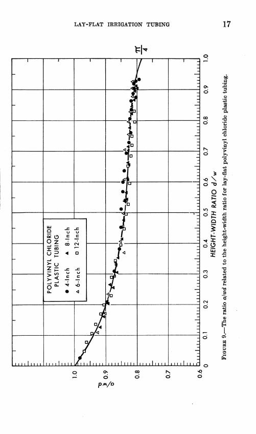
The cross-sectional area of a tube may be determined from the product of the tubing's height-width dimensions multiplied by some factor. As the tube becomes circular, the height and width dimensions each approach the diameter and the factor approaches 7r/4. With little or no hydrostatic.head, the tube cross section approaches that of a rectangle for which the factor approaches a value of unity. Quantitatively, this factor is a dimensionless number representing the ratio a/wd and is shown plotted versus tube shape, as represented by the height-width ratio (fig. 9). This curve was determined from the poly vinyl chloride plastic tube tests and will not apply to butyl

72^184 0—64 3


I

03

0/^ OIIV^ ^313\^VIQ-HiaiM tu P o


^h 1 J 1 1

1

TIT

TT

rTT

T

- 1 ^

-

«au

-f

- 1" •j ^

- •i

•r -^

- ^

PO

LY

VIN

YL

CH

LO

RID

E

PL

AS

TIC

T

UB

ING

• 4-I

nch

A B

-ln

ch

A 6-I

nch

°

12-I

nch

- f -^

-

t -£

- D/

1

-^

111111111 1 M i 1 1 1 1 1 /fl 1 1 1 1 1 1 1 11 111 1111 11 1 1111 1 1 ~l 1

i 1 1 1 1 M

Ö

00 Ö

d

a: J o O

CO

Ö

CN

Ö

Ö pM/o

GO

Ö d d

d

;3

o

q=l I

>> 03

O .2 ü «♦H

i I bc

5

I.


rubber tubing unless the side creases in the tubes have disappeared either through use or because of the fluid pressiu*e in the tube.

Effect of Fluid Density Upon Tube Shape

Corresponding data from tests conducted with fluids of difl^erent specific weights were also represented bv the curves shown in figures 4, 5, and 9 when the hydrostatic head was expressed as a cohunn height of the respective fluid. When the pressure head of the different fluids was expressed as the height of a column of water, however, there was a difference in the head-area relation, as shown in figure 10. In contrast to head-area curves, the individual curves representing the oil and brine fluids, in effect, are pressure-area curves for a particular fluid but generalized as to tube size. The three curves of figure 10 indicate that the greater the fluid density, the greater the pressure required to yield a given cross-sectional area.

The pressure head parameter H¡D is an abbreviated form of the p

parameter -^. When the tube area, represented by a/A, is plotted

P against —j^^ the resulting curve is a generalized pressure-area curve for

fluids of different density. When the parameter HjD is used in place

of -^, it is implied that H represents the hydrostatic head of the re-

spective fluid. When it does, the HID vs. ajA curve (solid line curve of fig. 10) is a generalized curve for different fluids. This is not true of the broken line curves of figure 10, since fl^for them does not represent their respective fluid but is expressed as a column height of water.

The variation in density of waters used for irrigation is relatively small. Therefore, when lay-flat tubing is used for irrigation, the effect of fluid density upon tube shape is so small that it becomes a matter of interest only and is not of practical significance.

DISCUSSION OF RESULTS

From the data that have been presented, it is possible to determine the cross-sectional area and describe the tube shape, as represented by the height-width ratio, for lay-flat tubing of any degree of roundaess. To do this, the full-round diameter must be known and any one of the following: tube height, tube width, or both, or the hydrostatic head. With the area ratio and the full-round area known, the tube cross- sectional area may be readily obtained.

With the area known, the mean flow velocity and the hydraulic radius are easily determined. The hydraulic radius may be obtained directly from the area ratio, since

£l—£.

where rjR is the ratio of the hydraulic radius for a tube at any shape to the hydraulic radius of a full-round pipe. Tube width, because of the influence of tubing wall thickness and stiffness, is not the best

LAT-FLAT IRRIGATION TUBING 19 O

■*»

03 ^J

O fg

1 S

o^ •ü o II en bC^

d la «g'o

a* N. l-s o fl^ o;^ feS

to o

■-s-S o •fia o < «t \ ss o «Ü o

•o ö <

QC 03 0)

< qq.ïï

LU bOTS o: .3*3 '^ <

o

•ai CO o 0) o

CN ^& Ö •S a>

•"7 ¿.d os —

11

a/H oiiv^ ^BiBWviaavBH

o

20 TECHNICAL BULLETIN 13 O 9, U.S. DEPT. AGRICULTURE

single parameter to use in determining the tube area. The HID vs. ajA curve (fig. 10) becomes very steep when the tubing approaches a circular shape. Therefore, special care must be exercised when the tube area is determined from this region of the curve.

The tube height is a good parameter from which to determine the area ratio throughout the entire shape range. For most applications, the curve in figure 4 showing the relation of hydrostatic head, tube height, area, and height-width ratio will find the most frequent use. Since these data were obtained with the tubing supported by a flat surface level in a direction perpendicular to the tube length, they are most applicable to tubes supported in this manner. This represents an ideal condition; further research will be needed to determine the deviation therefrom when a tube is supported by a rough or side sloping surface.

The cross-sectional area of tubing, 4 to 16 inches inside diameter, was computed for different degrees of tubing roundness and at different head-diameter and height-diameter ratios (table 2). These values are applicable to all types of lay-flat tubing when supported on a relatively flat surface except thick-walled tubing, such as butyl rubber approximately 6 inches and smaller in diameter. The cross- sectional area of this tubing may be slightly less than that indicated in the table.

FLOW TESTS The flow-testing phase of this study was undertaken to determine

the effect of tubing shape upon the friction coefficient and to obtain data from which the shape factor in equation 12 could be evaluated.

EXPERIMENTAL PROCEDURE

Flow tests were conducted with 6- and 8-inch nylon-supported polyvinyl chloride plastic experimental tubing. An 80-foot, slope adjustable ramp was used to support the tubes on which the flow tests were made (fig. 11). The tubing at the intake end was fastened to a 12-inch water supply line. Water from the tube discharged freely into an open flume at the lower end of the ramp. Flow rates of 1 c.f.s. and greater were measured with a 12-inch flowmeter installed in the supply line, whereas lesser flow rates were determined with a small weighing tank.

Coreless valve stems were secured to the bottom of the tube at 5-foot intervals along the test section. Clear plastic tubing connected the valve stems to a manometer board from which the piezometric pressure head at each 5-foot station was measured (fig. 12). Geo- metrical dimensions of the tube were measured during the tests. The tube height was measured with a point gage mounted on a stand that straddled the tube (fig. 13). The stand was also fitted with a scale with which to measure the horizontal width of the tubing. The perimeter varied slightly along the tube and, therefore, was measured with a small metallic rule at each station.

Tests were made on each tube, with the tube resting on a 0-, K-, 1-, and 2-percent slope. Runs were also made at zero slope with a 6-inch tube full round.

TABLE 2.- —Cross-section area of lay-flat tubing of different diameters ' at dijfferent degrees of roundness

Height- Area Head- Height- Cross-section area for tube size (inside diameter, inches)— width ratio diameter

ratio diameter

ratio ratio {dlw) {HID) WD) 4 6 8 10 12 14 16

Sq, ft. Sq.ft. Sq.ft. Sq.ft. Sq.ft. Sq.ft. Sq.ft. 1.000 1.000 1.000 0. 0873 0. 1963 0. 3491 0. 5454 0. 7854 1.069 1. 396 .975 .999 iÖ."9Ö" .985 .0872 .1962 . 3487 .5449 .7846 1.068 1.395 .950 .998 8.30 .968 .0871 . 1960 .3484 .5443 .7838 1.067 1.393 .925 .996 5.80 .953 . 0869 . 1956 .3477 .5432 .7822 1.065 1.391 .900 .994 4.35 .936 .0867 . 1952 .3470 .5421 .7807 1.063 1.388 .850 .986 2.90 .902 .0860 . 1936 .3442 .5378 .7744 1.054 1.377 .800 .976 2.14 .867 .0852 .1916 .3407 .5323 . 7666 1.043 1.363 .750 .962 1.70 .829 .0840 .1889 .3358 .5247 .7556 1.028 1.343 .700 .942 1.40 .790 .0822 . 1850 .3288 .5138 .7398 1.007 1. 315 .650 .921 1. 17 .750 .0804 . 1808 .3215 .5023 .7234 .985 1.286 .600 .895 1.01 .709 .0781 . 1757 .3124 .4881 .7029 .957 1.250 .550 .865 .88 .666 .0755 . 1698 .3019 .4718 .6794 .925 1.208 .500 .829 .77 .619 .0723 . 1628 .2894 .4521 .6511 .886 1. 157 .450 .787 .67 .571 .0687 . 1545 .2747 .4292 .6181 .841 1.099 .400 .742 .59 .520 .0648 . 1457 .2590 .4047 .5828 .793 1.036 .350 .686 .52 .467 .0589 . 1347 . 2395 .3742 .5388 .733 .958 .300 .624 .45 .409 .0544 . 1225 .2178 .3403 .4901 .667 .871 .250 .552 .37 .349 .0482 . 1084 . 1927 .3011 .4335 .590 .771 .200 .472 .29 .287 .0412 .0927 . 1648 .2574 .3707 .505 .659 . 150 .382 .22 .219 .0333 .0750 .1333 .2083 .3000 .408 .533 . 100 .275 .15 .150 .0240 .0540 .0960 . 1500 .2160 .294 .384 .050 . 150 .08 .076 .0131 .0294 .0524 .0818 .1178 .160 .209

0 0 0 0 0 0 0 0 0 0 0

s

£0

I i

i

^alA=r¡B. to

22 TECHNICAL BULLETIN 1309, V.S. DEPT. AGRICULTURE

FIGURE 11.—Slope adjustable ramp used in conducting flow tests on lay-ñat polyvinyl chloride plastic tubing.

DATA ANALYSIS AND PRESENTATION

The pipe equivalent relative roughness (e/Z?) was determined with data from the runs with the 6-inch plastic tube full round. The tubing boundary equivalent roughness («) was then calculated for that particular tubing material and found to be 3.2X 10~^ inches. Since both the 6- and 8-inch tubes were fabricated from the same material, the boundary roughness was the same for each.

It was necessary to determine the area at each 5-foot measuring station. The area ratio (a/A) was obtained with the use of a curve plotted from the hydrostatic test data relating tube height to the area. The height-diameter ratio (d/D), calculated from the tube measurements at each station, was the parameter used to determine the area ratio from this curve. The tube cross-sectional area was then computed for each station, and the mean flow velocity was determined from the continuity equation, Q=aV.

Some variation was noted in the velocity and hydraulic radius along the tube length. The discontinuities are attributed to variation in


'tmf^-

FIGURE 12.—Valve stem secured to the bottom of lay-flat poly vinyl chloride plastic tubing with a small plastic tube attached with which the pressure head was measured.

the tubing diameter, which variation was due to construction tech- nique and to pressure differences existing between the upper and lower ends of the tube during a test run. These variations were compen- sated for as much as possible by plotting the data versus distance along the tube. A curve was fitted to the data to obtain values representative of a tube of constant diameter.

Uniform Flow

The energy grade line was plotted for each run. At ramp slopes greater than zero, uniform flow was approached at the lesser flow rates. At uniform flow, the ramp slope was equal to the friction slope and the tube cross section remained constant throughout its length. The flow was also approximately uniform at some of the high flow rates


FIGURE 13.—Device used to measure the height and width of polyvinyl chloride plastic tubing during the flow tests. (Gravel was placed on the ramp after the flow tests reported herein were made.)

when the pressure was sufficient to maintain a near-round cross section. In general, however, the flow was nonimiform and the energy grade line was not straight but described an H-2, M-2, or M-Í surface profile curve, depending upon the ramp slope and flow rate.

For those runs where imiform flow was approached, the friction coefficient was determined with equation 10 in which

. SRghf J- ivi ' (22)


Nonuniform Flow

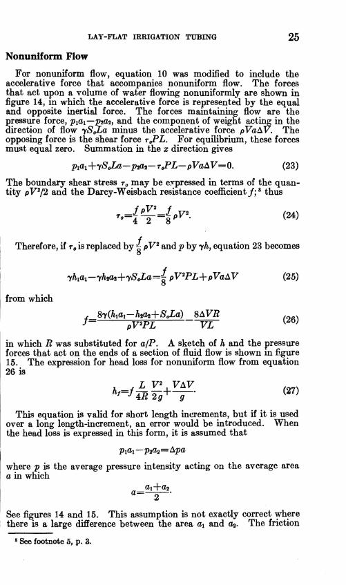
For nonuniform flow, equation 10 was modified to include the accelerative force that accompanies nonuniform flow. The forces that act upon a volume of water flowing nonimiformly are shown in figure 14, m which the accelerative force is represented by the equal and opposite inertial force. The forces maintaining flow are the pressure force, ^lai—^20^2, and the component of weight acting in the direction of flow ySJja minus the accelerative force pVaàV, The opposing force is the shear force TQPL, For equilibrium, these forces must equal zero. Summation in the x direction gives

Plal'\^ySoLa—p2(l^—ToPL—pVa^V=^Q. (23)

The boundary shear stress TQ may be expressed in terms of the quan- tity pF72 and the Darcy-Weisbach resistance coefl&cient /; ^ thus

Therefore, if TO is replaced by -¿ pV^ and 2? by 7Ä, equation 23 becomes o

lK<h.—ihßi-\-'iSjM=i pF'Pi+pFaAF (25)

from which

in which 22 was substituted for a¡F, A sketch of h and the pressure forces that act on the ends of a section of fluid flow is shown m fi,gure 15. The expression for head loss for nonuniform flow from equation 26 is

^'^UR2g^ g ^^^^

This equation is valid for short length increments, but if it is used over a long length-increment, an error would be introduced. When the head loss is expressed in this form, it is assumed that

where p is the average pressure intensity acting on the average area a in which

0= ;í • .2

See figures 14 and 15. This assumption is not exactly correct where there is a large difference between the area ai and a2. The friction

8 See footnote 5, p. 3.


/S^L«

FIGURE 14.—Sketch showing the forces acting on a section of nonuniform fluid flow.

M-*^ h = H-|- ^---^h, (AVERAGE PRESSURE ON END OF SECTION)

FIGURE 15.—Sketch showing the pressure forces acting on the ends of a flow tube.

coefficient, therefore, for nonuniform flow from the test data was evaluated with equation 26 rather than with equation 27.

The value of / computed from equation 26 generally decreased in value at consecutive stations along the tube toward the lower end. The value from which the shape factors were determined was the average value of / in the first 30 feet of the test section. Because of end effects, the data from stations near the end of the tube were not used to determine/.

Shape Factor Values of / determined from the experimental data with equations

22 and 26 were used to calculate values of ß with equation 11 in which

Values of /' were obtained from a pipe resistance diagram of friction coefficient versus Reynolds number. Coordinates for this diagram were computed with equations 4, 5, and 6. Values of/'were determined for a pipe of the same diameter and with the same relative roughness as the tubing if the tubing were round. The relative roughness was e/7?, where D was the full-round tube diameter, and was constant for each size of tube. Reynolds number for the tubing was conveniently computed from the following relationship :

VD áRV áaQ^4Q' 'vPa Pv R=- (28)


The shape factor ß is related to the tube shape, represented by the height-width ratio, and is shown by the curve in figure 16. The shape factor represents the effect upon head loss of the change in both velocity distribution and relative roughness caused by shape change.

The broken line curves shown in figure 16 indicate the trend of the curve beyond the data. Since a zero value of the ratio d/w represents a parallel boundary conduit of infinite extent, each end point curve was determined by evaluating the shape factor for parallel boundaries. This was accomplished by determining the ratio of the / value for {)araUel boundary flow to that of pipe flow at a given Reynolds number or different boundary spacings.

A definite end point at d/w=zeTo for the curve cannot be found, since the ///' ratio varies with Reynolds number. This variation results from the fact that the family of curves on the resistance diagrams are not parallel to each other from one value of Reynolds number to another. The Colebrook-White transition equation (equation 6) was modified for use with parallel boundary flow. This function, used to define / in the transition region between smooth and rough parallel boimdaries, was :

A resistance diagram for parallel boundaries was constructed by plotting values of /, computed with equations 7,8, and 29, versus Reynolds number for different values of relative roughness. The / values for paraUel boundary flow used in the ratio///' were taken from this resistance diagram.

Also shown in figure 16 is the calculated theoretical shape factor for laminar flow through an eUiptical-shaped conduit as given by Lamb ® in which

''=<^- <»>

This equation is included merely to show a comparison between the shape factor for laminar and turbulent flow through similarly shaped conduits.

With values of the shape factor ß known, equation 12 may now be used to represent the frictional head loss for uniform flow through lay- flat tubing.

DISCUSSION

Design Equations for Friction Loss The head loss for uniform flow through a tube may also be deter-

mined in terms of the loss for the same flow through a round rigid pipe of the same size and relative roughness. Since

4Ä IKar'JiAVV.'

(1)^ » LAMB« HORACE, HYDRODYNAMICS. Ed. 6, 587 pp., illus. New York. 1932.

1.4 1-

^1.3 -

oc O h« U 2 1.2 UJ

< CO

1.1

1.0

1 1—

POLYVINYL CHLORIDE PLASTIC ■ 6-lnch • 8-lnch

0.9

CALCULATED THEORETICAL FOR LAMINAR FLOW THROUGH AN ELLIPTICAL SHAPED CONDUIT

EVALUATED FOR PARALLEL BOUNDARIES

I I I I I I I I I I I I I M I I IM I t t I I I I I I I I I

■5^"^^v«

I I 1 I i M I I I I I I I M I I I » I I I I I I I

0.1 0.2 0.8 0.9 0.3 0.4 0.5 0.6 0.7 HEIGHT-- WIDTH RATIO d/w

FIGURE 16.—The shape factor ß related to the height-width ratio for lay-flat polyvinyl chloride plastic tubing.


equation 10 may be expressed in the following fonn:

^^K^Pñi-g- (31)

A convenient form, tb#i>ef0rd/ m wkfeh to express equation 12 for the head loss through lay-flat tubing is

— j is constant for any given tube shape and i IS re-

lated to the height-width ratio and the head-diameter ratio by the curve shown in figure 17. The loss for uniform flow through a tube may be determined by multiplying the loss for the same flow through a round

pipe by the factor i^ Í — ) • Equation 32 will probably be the simplest

and most practical form to use in designing and evaluating lay-flat tubing for field appUcation.

If the head loss were to be expressed in the form of equation 1, the equation appKcable to lay-flat tubing would be

.,=.(4) A\n+m KLV "" ^ ^^ (33)

in which values of K, Vp, and D are those applicable to the same flow through a pipe of the same size and roughness as the tube when round.

Use of the friction coefficient/' may in some cases introduce a small error, since it is determined from the Colebrooke-White transition curve on the pipe resistance diagram. This curve is for flow through a pipe of commercial or nonuniform roughness. For tubing that is not hydraulically smooth, the absolute roughness of the material from which it is fabricated will, in most cases, be more uniform than that of commercial pipe. Because of this, the /-Reynolds number relationship may depart slightly from the transition curve toward the curve pattern obtained by Nikuradse^^ in his experiments on pipe of uniform roughness. In most cases the error will likely be very small.

Relative Roughness

As noted previously (p. 2), the tubing relative roughness is affected by a shape change and is difficult to define. For a tube shape in- between the two limits of pipe and parallel boundaries, the depth of flow midway between boundaries is different in the width direction from that in the height direction. The problem, therefore, is to represent the two flow depths by a single dimension that will be valid from one shape limit to the other. Four times the hydraulic radius

1Ö See footnote 5.


a/H OI1VÎI îi3i3wvia-av3H o o o

^ CO 9 »n CM ^

o ^ CO ^00

I 1 Mil 1 1 1 1 III 1

I n

\

i h /

-_

/

^

} /

/

I

Á f /

~

i ULXJ.

/

III 1 1 J_I_L.LI,I ILL 1 i 1 1 1 1 1 1 1 1 II 1 i 11 1 i~

<|o

I ^ ^

a» Ö

00

Ö d d d

13

03

bO

3

03 Cd

^|ö

oa

H

g M

/^/P OIIVH HiaiM-lHOI3H


is often used to represent this characteristic length. This is valid for open channel flow, but for closed conduits, use of the hydraulic radius introduces an error of two as the cross section approaches the parallel-boundary shape Umit. At this limit, the actual relative roughness is two times as great as that indicated when four times the hydrauUc radius is used in its determination.

^ The relative roughness for a circular shape is represented by

€/Z?=c/4Ä,

whereas for parallel boundaries it is represented by

€/fi=€/2Ä.

In the absence of more precise information, the tube height d would Hkely be the best parameter from which to compute the actual tubing relative roughness. Use of this dimension would give the correct value when the tube is full round and also as it approaches a rectangular shape, even though it may not be exactly correct at shapes in-between these two limits.

The effect of relative roughness, as related to tube shape, upon the friction coefficient is not separately evaluated in this bulletin but is included in the shape factor ß. The hydraulic design is thereby made easier because the roughness value used in determining /' is constant for each tube irrespective of tube shape. If the effect of relative roughness upon head loss were to be represented by the friction coefficient jf' instead of ß^ j' would be determined from a resistance diagram in which the tubing relative roughness would be computed from a representative tube dimension such as tube height. In this case a different shape factor would be required, since the relative roughness effect would be included in f rather than in the shape factor.

Further Study Needed

The effect of ground surface roughness upon flow through lay-flat tubing may exceed the shape effects. This problem has not yet been studied. The initial laboratory investigation reported herein needs to be supplemented by further study in the field.

The nonuniform flow phase of the problem and the effects of accel- erated flow near the end of the tube need further study.

Additional information is needed to determine more fully the requirements and performance characteristics of lay-flat tubing materials. Further development of tubing outlets and couplings with their hydrauhc characteristics is needed.

DISCHARGE DIAGRAMS

Typical diagrams relating the discharge to the head loss for irrigation tubing of different diameters and degrees of roundness are shown in figures 18 to 22. These diagrams show the influence of tube shape


20

2 3 4 5 6 8 10 20 HEAD LOSS PER 1000 FEET - FEET

30 40

FIGURE 18.—^Head-discharge diagram for lay-flat irrigation tubing with smooth boundaries for different degrees of roundness.

upon the discharge for tubes having a boundary varying from smooth to 0.003 inch equivalent roughness. The curves in these figures were computed with equation 32. To use the diagram for tubes at less than a full-round cross section, it is necessary to know the pressure head in the tube. In designing for imiform flow on sloping ground,


2 3 4 5 6 8 10 20 30 40 HEAD LOSS PER 1000 FEET - FEET

FIGURE 19.—Head-discharge diagram for lay-flat irrigation tubing, e=0.0004 inch, for different degrees of roundness.

this may be assumed, in most cases, to be the same as the head on the tube at the intake end. The capacity of a tube flowing at less than full-round may be increased by providing for additional head to bring the tube to a more round cross section; a margin of safety may therefore be provided.


20


FIGURE 20.—Head-discharge diagram for lay-flat irrigation tubing, €=0.001 inch, for different degrees of roundness.

Care is needed in using the discharge diagrams for tubing on rough ground surfaces. The friction coefficient does not include the effect of ground surface roughness upon the head loss. Therefore, a margin of safety must be provided by the designer until adequate information is available to evaluate accurately this effect.


1 2 3 4 5 6 8 10 20 30 40 HEAD LOSS PER 1000 FEET - FEET

FIGURE 21.—Head-discharge diagram for lay-flat irrigation tubing, €=0.002 inch, for different degrees of roundness.

Examples are presented to illustrate how figures 18 to 22 ina.j be used in the design of tubing on a smooth groimd surface. Minor head losses such as entrance and coupler loss have been omitted to simplify the ülustrations.


20


FIGURE 22.—^Head-discharge diagram for lay-flat irrigation tubing, €=0.003 inch, for different degrees of roundness.

Problem: Determine the ground slope required to maintain imiform flow of 2 c.f.s. flowing through a 10-inch-diameter tube having a roughness of 0.003 inch, with a head of 2 feet provided at the intake.

H 24 Head-diameter ratio y^=Tyr=2.4.


From figure 22 the head loss would be 4.8 feet per 1,000 feet or a slope of 0.0048.

Problem: If we assume flow is imiform, what size tube will be required to carry 3 c.f.s. at a ground slope of 0.5 percent with a 2-foot head available at the intake. Try a 124nch tube:

Head loss per 1,000 feet equals 5 feet. From figure 22 the discharge equals 3.25 cf.s. A 12-inch tube therefore will be adequate (if tubing boundary roughness is assumed equal to 0.003 inch).

SUMMARY

STATIC TESTS

The hydraulic properties of lay-flat irrigation tubing are closely related to the shape and cross-sectional area of the tube. These characteristics are m turn dependent upon the fluid pressure head inside the tube. A study was imdertaken to obtain data from which the pressure-shape-area relations could be determined. The cross section of tubing at various hydrostatic pressure heads was traced with a special pantograph. Tracings were made on supported poly vinyl chloride plastic and butyl rubber tubes of different diameters. The area of the cross-sectional tracings was measured and related to the hydrostatic head, tube height, width, height-width ratio, and height- width product. The results, expressed in dimensionless ratios, are shown in figures 4 to 10.

The cross-sectional area of tubing 4 to 16 inches in diameter for different degrees of tubing roundness was determined and is presented in table 2.

FLOW TESTS

A study was also undertaken to determine the effect of tube shap © upon the frictional head loss. Flow tests were conducted on 6- and 8-inch nylon-supported polyvinyl chloride experimental tubing. Frictional head loss for imiform flow through the tubing was expressed in the form of the Darcy-Weisbach equation in which

The frictional head loss for nonimiform flow was erpressed by a modified form of the Darcy-Weisbach equation in which

. , L V'.VAV

The friction coefficient/ is equal to ßf^ where j8 is a shape factor that varies with tube shape. The friction coefficient/' is for an equivalent


flow through a rigid pipe of the same diameter as the tube and was determined from a conventional pipe resistance diagram.

The head loss for uniform flow through tubing, when compared to the same flow through a round pipe of the same size and roughness,

varied as the product of ßy — )'

Diagrams relating the discharge for irrigation tubing of d fferent diameters and degrees of roundness to the head loss are presented.

SYMBOLS AND DEFINITIONS Symbol Dimension Definition A L2 Cross-sectional area of a circular flow conduit and of a

flexible tube when fully round. a L* Cross-sectional area of tube when less than full round. B L Parallel boundary spacing. D L Diameter of a circular flow conduit and of a flexible tube

when fully round. d L Vertical height of a tube or flow conduit. / Friction coefficient. /' Friction coefficient for a full-round tube or for a rigid

pipe of the same diameter and roughness, and at the same Reynolds number and equivalent flow as the tube

G Specific gravity. g L/T^ Acceleration of gravity=32.2 ft./sec.« H L Pressure head of fluid in the tube. h L Pressure head used in computing the force on the end ol

an increment of tube length and is equal to H—d/2. hf L Frictional head loss. K Constant. k, € L Boundary roughness dimension. e/d Tubing equivalent relative roughness. e/D Equivalent relative roughness for pipe or fully round

tube. L L Length. P L Perimeter. p F/L^ Pressure intensity. Q L^T Rate of flow.

R L Hydraulic radius = —:—7— •^ perimeter R Reynolds number. r L Hydraulic radius of tube at less than round shape when

used in ratio r/R. To L Radius of a circular conduit. So Slope of ramp on which tube rested during the flow tests. V LIT Actual mean velocity. 1 Fp LjT Mean velocity for an equivalent flow through a round

pipe. ß Shape factor. y FjU Specific weight of water=62.4 Ib./ft.' | V L^/T Kinematic viscosity, p FT^/L^ Density. TO F/L^ Boundary shear stress.

U.S. GOVERNMENT PRINTING OFFICE : 1964 O—726-184

D 5566