lateral reaction jet flow interaction effects on a generic … reaction jet flow interaction effects...

Lateral Reaction Jet Flow Interaction Effects on a Generic

Fin-Stabilized Munition in Supersonic Crossflows

by James DeSpirito

ARL-TR-6707 November 2013 Approved for public release; distribution is unlimited.

NOTICES

Disclaimers The findings in this report are not to be construed as an official Department of the Army position unless so designated by other authorized documents. Citation of manufacturer’s or trade names does not constitute an official endorsement or approval of the use thereof. Destroy this report when it is no longer needed. Do not return it to the originator.

Army Research Laboratory Aberdeen Proving Ground, MD 21005-5066

ARL-TR-6707 November 2013

Lateral Reaction Jet Flow Interaction Effects on a Generic Fin-Stabilized Munition in Supersonic Crossflows

James DeSpirito

Weapons and Materials Research Directorate, ARL Approved for public release; distribution is unlimited.

ii

REPORT DOCUMENTATION PAGE Form Approved OMB No. 0704-0188

Public reporting burden for this collection of information is estimated to average 1 hour per response, including the time for reviewing instructions, searching existing data sources, gathering and maintaining the data needed, and completing and reviewing the collection information. Send comments regarding this burden estimate or any other aspect of this collection of information, including suggestions for reducing the burden, to Department of Defense, Washington Headquarters Services, Directorate for Information Operations and Reports (0704-0188), 1215 Jefferson Davis Highway, Suite 1204, Arlington, VA 22202-4302. Respondents should be aware that notwithstanding any other provision of law, no person shall be subject to any penalty for failing to comply with a collection of information if it does not display a currently valid OMB control number. PLEASE DO NOT RETURN YOUR FORM TO THE ABOVE ADDRESS.

1. REPORT DATE (DD-MM-YYYY)

November 2013 2. REPORT TYPE

Final 3. DATES COVERED (From - To)

November 2010–December 2011 4. TITLE AND SUBTITLE

Lateral Reaction Jet Flow Interaction Effects on a Generic Fin-Stabilized Munition in Supersonic Crossflows

5a. CONTRACT NUMBER

5b. GRANT NUMBER

5c. PROGRAM ELEMENT NUMBER

6. AUTHOR(S)

James DeSpirito

5d. PROJECT NUMBER

AH80 5e. TASK NUMBER

5f. WORK UNIT NUMBER

7. PERFORMING ORGANIZATION NAME(S) AND ADDRESS(ES)

U.S. Army Research Laboratory ATTN: RDRL-WML-E Aberdeen Proving Ground, MD 21005-5066

8. PERFORMING ORGANIZATION REPORT NUMBER

ARL-TR-6707

9. SPONSORING/MONITORING AGENCY NAME(S) AND ADDRESS(ES)

10. SPONSOR/MONITOR’S ACRONYM(S)

11. SPONSOR/MONITOR'S REPORT NUMBER(S)

12. DISTRIBUTION/AVAILABILITY STATEMENT

Approved for public release; distribution is unlimited.

13. SUPPLEMENTARY NOTES

Presented as paper AIAA-2011-3031 at the 29th AIAA Applied Aerodynamics Conference, Honolulu, HI, 27–30 June 2011, and paper AIAA-2012-0413 at the 50th AIAA Aerospace Sciences Meeting, Nashville, TN, 9–12 January 2012. 14. ABSTRACT

The flow interaction effects from a jet issuing into a supersonic crossflow were investigated computationally for the case of a flat plate and a generic fin-stabilized projectile. For both configurations, simulations were performed at several Mach numbers and jet total to freestream static pressure ratios (PRs). In the flat plate case, the jet force was generally amplified, with a strong dependence on PR and the freestream Mach number. In the projectile configuration, seven jet locations along the missile axis were investigated at three supersonic crossflow Mach numbers and five angles of attack in the range –10° ≤ ≤ 10°. The jet force was generally attenuated, unless the jet was located very close to the tail fins. In the latter case, this results from (1) a combination of little or no projectile surface area for the detrimental jet interaction effects to act on, and (2) the high pressures developed on the fin surfaces. The choice of turbulence model was found to affect the local pressure distribution due to the flow interaction, but the jet interaction force parameters varied less than 15% and 6% for the flat plate and missile configurations, respectively. The effect of angle of attack on jet interaction forces was more prevalent as became more negative and the counter-rotating vortex pair in the jet plume was pushed closer to the tail fins. Flight simulations using reaction jet “squibs” were performed to evaluate the sensitivity of the control maneuver to the differences in jet thrust and jet actuation location. These results showed that significant differences in the projectile maneuver control were obtained if the effective jet thrust acting at the effective jet location were used instead of the ideal jet thrust acting at the jet exit location. 15. SUBJECT TERMS

reaction jet control, CFD, jet interaction, aerodynamics, Army-Navy Finner, supersonic crossflow

16. SECURITY CLASSIFICATION OF: 17. LIMITATION OF ABSTRACT

UU

18. NUMBER OF PAGES

116

19a. NAME OF RESPONSIBLE PERSON

James DeSpirito a. REPORT

Unclassified b. ABSTRACT

Unclassified c. THIS PAGE

Unclassified 19b. TELEPHONE NUMBER (Include area code)

410-306-0778 Standard Form 298 (Rev. 8/98)

Prescribed by ANSI Std. Z39.18

iii

Contents

List of Figures v

List of Tables viii

Acknowledgments xii

1. Introduction 1

2. Numerical Approach 4

2.1 Flat Plate Model ..............................................................................................................4

2.2 Army-Navy Finner Model ...............................................................................................7

2.3 Computational Details ...................................................................................................11

3. Results and Discussion 12

3.1 Flat Plate Case ...............................................................................................................13

3.1.1 Grid Resolution Study .......................................................................................13

3.1.2 Turbulence Model Study ...................................................................................14

3.1.3 Nozzle Parameter Study ....................................................................................20

3.2 Army-Navy Finner Test Case ........................................................................................25

3.2.1 Turbulence Model Investigation .......................................................................26

3.2.2 = 0° Cases ......................................................................................................28

3.2.3 Effect of on JI.................................................................................................45

3.2.4 Flight Trajectory Simulations ............................................................................54

4. Summary and Conclusions 60

5. References 63

Appendix A. Army-Navy Finner With No Jet Validation 67

Appendix B. Army-Navy Finner Tabulated Results at = 0° 69

Appendix C. Army-Navy Finner Tabulated Results at = ±10° 81

iv

Appendix D. Army-Navy Finner Tabulated Results at = ±5° 87

Appendix E. Army-Navy Finner Tabulated Results at = ±2.5° 93

List of Symbols, Abbreviations, and Acronyms 97

Distribution List 101

v

List of Figures

Figure 1. Accepted flow structure of jet injecting into a supersonic crossflow from a flat plate. ...........................................................................................................................................2

Figure 2. Schematic of a JI flowfield around a body of revolution. ................................................2

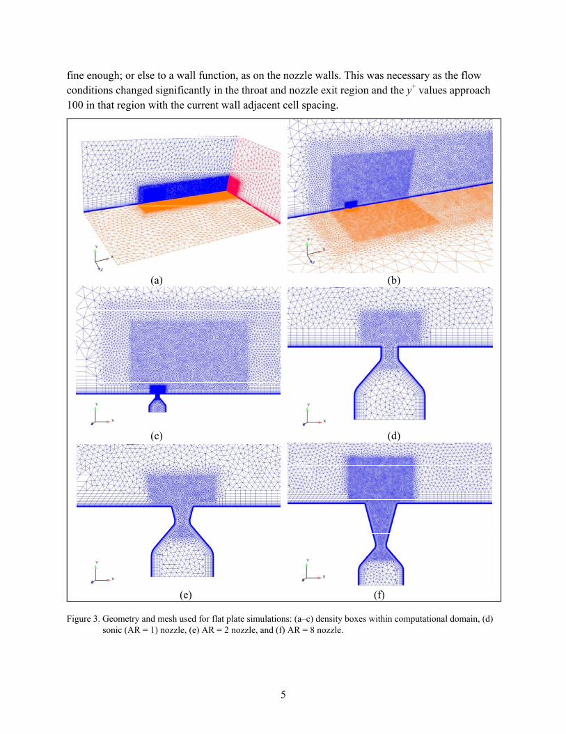
Figure 3. Geometry and mesh used for flat plate simulations: (a–c) density boxes within computational domain, (d) sonic (AR = 1) nozzle, (e) AR = 2 nozzle, and (f) AR = 8 nozzle. ........................................................................................................................................5

Figure 4. ANF (Basic) missile geometry (dimensions in cal., d 30 mm). ......................................8

Figure 5. Geometry and mesh used for ANF simulations: (a) symmetry plane of computational domain, (b) density boxes for F0 jet location, (c) density boxes for F2 jet location, (d) sonic nozzle, (e) surface mesh near nozzle exit, and (f) surface meshes on projectile and symmetry plane. ................................................................................................10

Figure 6.Comparison of normalized pressure profiles on flat plate for run no. 26-6 (Mach 2.61): (a) along plate centerline, forward and rearward of jet, and (b) laterally to the side of the jet orifice. .......................................................................................................................14

Figure 7. Comparison of normalized pressure profiles on flat plate for run 30-5 (Mach 2.01): (a) along plate centerline, forward and rearward of jet, and (b) laterally, to the side of the jet..............................................................................................................................................16



Figure 10. Comparison of normalized pressure profiles on flat plate for run 19-2 (Mach 4.54): (a) along plate centerline, forward and rearward of jet, and (b) laterally, to the side of the jet. ..................................................................................................................................19

Figure 11. Flowfield around jet issuing from flat plate at (a) Mach 1.7 and (b) Mach 2.5. Shown are Mach number contours on symmetry and far field planes and normalized pressure contours on plate surface. ..........................................................................................21

Figure 12. Force amplification factor variation with Mach number and AR for flat plate simulations, (a) PR=340, (b) PR=148, (c) PR=49, and (d) variation with PR and AR at Mach 2.5. .................................................................................................................................24

Figure 13. Force amplification factor variation with PR and (a) jet gas total temperature and (b) freestream conditions (altitude), at Mach 2.5. ....................................................................25

Figure 14. Comparison of normalized pressure profiles on ANF projectile surface (a, b) longitudinally on upper surface along projectile axis, and (c) azimuthally in axial plane of jet, M = 1.5, = 0. ..................................................................................................................27

vi

Figure 15. Normalized pressure on projectile surfaces and Mach number on symmetry plane in region near the jet (jet location F0) in (a) Mach 1.5 and (b) Mach 2.5 crossflows. ............28

Figure 16. Pressure ratio on projectile surfaces, Mach number on symmetry plane for (a) Mach 1.5, (b) Mach 2.5, and (c) Mach 3.5; F0 jet exit location, = 0 (scales: 0.5 ≤ p/p∞ ≤ 2.0; 0 ≤ M ≤ 10.0). ...................................................................................................................29

Figure 17. Normalized pressure on projectile surface and Mach number on symmetry plane for jet locations (from top) F3, F2, F1, F0, R1, R2, R3 and Mach (a) 2.5 and (b) 1.5 (scales: 0.5 ≤ p/p∞ ≤ 2.0; 0 ≤ M ≤ 10.0). ..................................................................................30

Figure 18. Normalized pressure on projectile surfaces and vorticity contours on axial plane locations (a) F3, (b) F2, (c) F1, (d) R1, (e) R2, and (f) R3 at Mach 2.5 (scales: 0.5 ≤ p/p∞

≤ 2.0; 0 ≤ ≤ 500,000). ...........................................................................................................31

Figure 19. Normalized pressure on projectile surfaces and vorticity contours on axial plane locations (a) F3, (b) F2, (c) F1, (d) R1, (e) R2, and (f) R3 at Mach 1.5 (scales: 0.5 ≤ p/p∞

≤ 2.0; 0 ≤ ≤ 500,000). ...........................................................................................................32

Figure 20. JI (a) force and (b) moment distributions along projectile body for specified jet locations (Mach 2.5, PR = 340). ..............................................................................................33

Figure 21. Normalized pressure along projectile (a) upper and (b) lower surfaces for specified jet locations (Mach 2.5, PR = 340). .........................................................................................34

Figure 22. (a) Force and (b) moment amplification factors as function of jet location (PR = 340). .........................................................................................................................................35

Figure 23. Force coefficients as function of jet location at Mach (a) 1.5, (b) 2.5, and (c) 3.5 (PR = 340). ...............................................................................................................................37

Figure 24. Moment coefficients as function of jet location at Mach (a) 1.5, (b) 2.5, and (c) 3.5 (PR = 340). ...............................................................................................................................38

Figure 25. Force center of pressure as function of jet location at Mach (a) 1.5, (b) 2.5, and (c) Mach 3.5 (PR = 340). ...............................................................................................................39

Figure 26. (a) Force and (b) moment amplification factors as function of jet location at Mach 1.5 (PR = 340). .........................................................................................................................41

Figure 27. (a) Force and (b) moment amplification factors as function of jet location at Mach 2.5 (PR = 340). .........................................................................................................................42

Figure 28. Force amplification factor as function of jet location and PR at Mach (a) 2.5 and (b) 1.5 (AR = 1). ......................................................................................................................43

Figure 29. Force amplification factor as function of jet location and AR (a) PR=340, (b) PR = 148, and (c) PR = 49 (Mach 2.5). .........................................................................................44

Figure 30. Pressure ratio on projectile surfaces, Mach number on symmetry plane (left) and vorticity contours on axial planes (right) for Mach 2.5, F0 jet exit location, (a) = –10, (b) = –5, (c) = 0, (d) = 5, and (e) = 10 (Scales: 0.5 ≤ p/p∞ ≤ 2.0; 0 ≤ M ≤ 10.0). ..........................................................................................................................46

Figure 31. Pressure ratio on projectile surfaces, Mach number on symmetry plane (left) and vorticity contours on axial planes (right) for Mach 2.5, F3 jet exit location, (a) = –10, (b) = –5, (c) = 0, (d) = 5, and (e) = 10 (Scales: 0.5 ≤ p/p∞ ≤ 2.0; 0 ≤ M ≤ 10.0). ..........................................................................................................................47

vii

Figure 32. Pressure ratio on projectile surfaces, Mach number on symmetry plane (left) and vorticity contours on axial planes (right) for Mach 2.5, R3 jet exit location, (a) = –10, (b) = –5, (c) = 0, (d) = 5, and (e) = 10 (Scales: 0.5 ≤ p/p∞ ≤ 2.0; 0 ≤ M ≤ 10.0). ..........................................................................................................................48

Figure 33. Pressure ratio on projectile surfaces, Mach number on symmetry for Mach 1.5 (left) and 3.5 (right), F0 jet exit location, (a) = –10, (b) = 0, and (c) = 10 (Scales: 0.5 ≤ p/p∞ ≤ 2.0; 0 ≤ M ≤ 10.0). ..................................................................................49

Figure 34. Pressure ratio on projectile surfaces, Mach number on symmetry for Mach 1.5 (left) and 3.5 (right), F3 jet exit location, (a) = –10, (b) = 0, and (c) = 10 (Scales: 0.5 ≤ p/p∞ ≤ 2.0; 0 ≤ M ≤ 10.0). ..................................................................................49

Figure 35. (a) Force and (b) moment amplification factor vs. , Mach 1.5. .................................50



Figure 38. Effective jet location (cal.) vs. , (a) Mach 1.5, (b) Mach 2.5, and (c) Mach 3.5. ......53

Figure 39. Extended range trajectory simulation at Mach 1.5 for jet at F3 location: (a) altitude vs. range, and (b) total angle of attack vs. range. .....................................................................58

Figure 40. Left deflection trajectory simulation at Mach 1.5: deflection vs. range for jet at (a) F3 location, (b) R3 location, and (c) total angle of attack vs. range for jet at R3 location. .....59

Figure A-1. Comparison of predicted and experimental normal force coefficient for ANF with no jet. ...............................................................................................................................68

Figure A-2. Comparison of predicted and experimental pitching moment coefficient for ANF with no jet. ...............................................................................................................................68

viii

List of Tables

Table 1. Flow conditions of flat plate validation simulations. .........................................................6

Table 2.Flow conditions used in flat plate nozzle parameter study (sonic jet, AR = 1). .................7

Table 3. Jet locations along ANF projectile. ....................................................................................8

Table 4. Comparison of PRs ( = 34.5 MPa, = 1.28 × 107 Pa). .............................................11

Table 5. Results from turbulence model study. .............................................................................20

Table 6. Results from nozzle parameter study at STP freestream conditions ( 0 =300 K). .........22

Table 7. Results from nozzle parameter study, variation with jet gas total temperature (AR=1, M=2.5, STP freestream conditions). .......................................................................................22

Table 8. Results from nozzle parameter study, variation with altitude, (AR=2, M=2.5, 0 =300 K). .............................................................................................................................23

Table 9. Results from turbulence model study (F2 jet location, M = 1.5, = 0, = 215.6 N). ............................................................................................................................................28

Table 10. Force and moment amplification factors vs. Mach number and jet location (PR = 340). .........................................................................................................................................36

Table 11. Results of trajectory simulations for extended range maneuver, Fj = 215.6 N. ............55

Table 12. Results of trajectory simulations for left deflection maneuver, Fj = 215.6 N. ..............56

Table B-1. Amplification factor, normal force, and pitching moment results as function of jet location on ANF body-tail configuration (M = 1.5, PR = 340, AR = 1, = 0°). ....................70

Table B-2. Center of pressure results as function of jet location on ANF body-tail configuration (M = 1.5, PR = 340, AR = 1, = 0°). ...............................................................70





Table B-7. Amplification factor, normal force, and pitching moment results as function of jet location on ANF body-alone configuration (M = 1.5, PR = 340, AR = 1, = 0°). .................72

Table B-8. Amplification factor, normal force, and pitching moment results as function of jet location on ANF body-alone configuration (M = 2.5, PR = 340, AR = 1, = 0°). .................72


Table B-10. Center of pressure results as function of jet location on ANF body-tail

ix

configuration (M = 1.5, PR = 148, AR = 1, = 0°). ...............................................................73

Table B-11. Amplification factor, normal force, and pitching moment results as function of jet location on ANF body-tail configuration (M = 2.5, PR = 148, AR = 1, = 0°). ...............73


Table B-13. Amplification factor, normal force, and pitching moment results as function of jet location on ANF body-tail configuration (M = 1.5, PR = 49, AR = 1, = 0°). .................74

Table B-14. Center of pressure results as function of jet location on ANF body-tail configuration (M = 1.5, PR = 49, AR = 1, = 0°). .................................................................74




Table B-18. Center of pressure results as function of jet location on ANF body-tail configuration (M = 2.5, PR = 340, AR = 2, = 0°). ..............................................................75




Table B-22. Center of pressure results as function of jet location on ANF body-tail configuration (M = 2.5, PR = 49, AR = 2, = 0°). ................................................................77







Table C-1. Amplification factor, normal force, and pitching moment results as function of jet location on ANF body-tail configuration (M = 1.5, PR = 340, AR = 1, = –10°). ................82

Table C-2. Center of pressure results as function of jet location on ANF body-tail

x

configuration (M = 1.5, PR = 340, AR = 1, = –10°). ...........................................................82

Table C-3. Amplification factor, normal force, and pitching moment results as function of jet location on ANF body-tail configuration (M = 1.5, PR = 340, AR = 1, = 10°). ..................82

Table C-4. Center of pressure results as function of jet location on ANF body-tail configuration (M = 1.5, PR = 340, AR = 1, = 10°). .............................................................83

Table C-5. Amplification factor, normal force, and pitching moment results as function of jet location on ANF body-tail configuration (M = 2.5, PR = 340, AR = 1, = -10°). .................83

Table C-6. Center of pressure results as function of jet location on ANF body-tail configuration (M = 2.5, PR = 340, AR = 1, = -10°). ............................................................83

Table C-7. Amplification factor, normal force, and pitching moment results as function of jet location on ANF body-tail configuration (M = 2.5, PR = 340, AR = 1, = 10°). ..................84


Table C-9. Amplification factor, normal force, and pitching moment results as function of jet location on ANF body-tail configuration (M = 3.5, PR = 340, AR = 1, = –10°). ................84

Table C-10. Center of pressure results as function of jet location on ANF body-tail configuration (M = 3.5, PR = 340, AR = 1, = –10°). ...........................................................85

Table C-11. Amplification factor, normal force, and pitching moment results as function of jet location on ANF body-tail configuration (M = 3.5, PR = 340, AR = 1, = 10°). .............85


Table D-1. Amplification factor, normal force, and pitching moment results as function of jet location on ANF body-tail configuration (M = 1.5, PR = 340, AR = 1, = –5°). ..................88

Table D-2. Center of pressure results as function of jet location on ANF body-tail configuration (M = 1.5, PR = 340, AR = 1, = –5°). .............................................................88

Table D-3. Amplification factor, normal force, and pitching moment results as function of jet location on ANF body-tail configuration (M = 1.5, PR = 340, AR = 1, = 5°). ....................88

Table D-4. Center of pressure results as function of jet location on ANF body-tail configuration (M = 1.5, PR = 340, AR = 1, = 5°). ...............................................................89


Table D-6. Center of pressure results as function of jet location on ANF body-tail configuration (M = 2.5, PR = 340, AR = 1, = –5°). .............................................................89

Table D-7. Amplification factor, normal force, and pitching moment results as function of jet location on ANF body-tail configuration (M = 2.5, PR = 340, AR = 1, = 5°). ....................90



Table D-10. Center of pressure results as function of jet location on ANF body-tail

xi

configuration (M = 3.5, PR = 340, AR = 1, = –5°). .............................................................91

Table D-11. Amplification factor, normal force, and pitching moment results as function of jet location on ANF body-tail configuration (M = 3.5, PR = 340, AR = 1, = 5°). ...............91


Table E-1. Amplification factor, normal force, and pitching moment results as function of jet location on ANF body-tail configuration (M = 2.5, PR = 340, AR = 1, = –2.5°). ...............94

Table E-2. Center of pressure results as function of jet location on ANF body-tail configuration (M = 2.5, PR = 340, AR = 1, = –2.5°). ..........................................................94

Table E-3. Amplification factor, normal force, and pitching moment results as function of jet location on ANF body-tail configuration (M = 2.5, PR = 340, AR = 1, = 2.5°). .................95

Table E-4. Center of pressure results as function of jet location on ANF body-tail configuration (M = 2.5, PR = 340, AR = 1, = 2.5°). ............................................................95

xii

Acknowledgments

This work was supported in part by grants of high-performance computing time from the U.S. Department of Defense (DOD) High Performance Computing Modernization program at the U.S. Army Research Laboratory (ARL) DOD Supercomputing Resource Center (DSRC), Aberdeen Proving Ground, MD, and the Air Force Research Laboratory DSRC, Wright-Patterson Air Force Base, OH. The author would also like to thank Ms. Karen Heavey for providing a technical review of the manuscript.

1

1. Introduction

The study of jets issuing into a crossflow has been the subject of research for about 70 years (1–3). The primary purpose of such a reaction jet control (RJC) system is to generate a lateral force or moment to provide attitude or roll control for a flight vehicle. There are several advantages of RJC systems over conventional aerodynamic controls such as canards or fins; e.g., increased maneuver authority when operating in low dynamic pressure (low velocity or high altitude), small time delay for the actuation effect, and compact design. In addition, the external aerodynamics of the flight vehicle is unaffected except during the actuation period of the jet. The main disadvantage of an RJC system is the effect of the jet interaction (JI) flowfield on the control forces and moments. Research shows that the operation of a lateral reaction jet in atmospheric flight results in an interference flow between the jet plume and the flow over the vehicle (2, 3). The JI effect increases the difficulty of determining simple models of RJC systems to apply the technology (4).

The study of reaction jet interaction effects is still an active area of research. Some recent computational studies include the shock-boundary layer interaction effects on a flat plate (5) and a body of revolution (6), and experimental and computation results on a flat plate (7) and generic missile configurations (8–14). Experimental studies including particle image velocimetry (PIV) measurements on a flat plate (15–17) and a missile configuration (18, 19) provide valuable information on the flowfield structure away from the body surfaces.

The currently accepted flow structure in the near field of a supersonic jet issuing into a supersonic crossflow is illustrated in figure 1, as presented by Champigny and Lacau (3) for a flow over a flat plate. One of the main features is due to the jet stream acting as an obstruction to the flow. A shock-boundary layer interaction forms upstream of the jet as the approaching boundary layer interacts with the bow shock, leading to a -shock structure. The separated flow in this region wraps around the jet and forms the counter-rotating horseshoe vortices that stay near the wall surface. The jet plume is curved in the direction of the flow due to the freestream crossflow. A “barrel” shock surrounds the jet plume and terminates in a Mach disk. Two counter-rotating wake vortices form and travel downstream as the primary flow feature of the jet plume. These vortices likely originate from the ring vortices of the jet shear layer as they exit the orifice, which get transformed as they interact with the crossflow (3).

The flow structure in the near field of a supersonic jet issuing from a body of revolution, i.e., a projectile or missile, is similar to that for the flat plate and is shown in figure 2. Some differences are that the jet is now located behind the bow shock formed at the nose of the projectile. Also, the jet bow shock and horseshoe vortices emanating from the separation region will tend to

2

“wrap around” the projectile body. The basic features of the separation region and -shock are very similar to that observed with a jet issuing from a flat plate. A strong turbulent wake extends behind the jet and a recompression shock forms downstream.

Figure 1. Accepted flow structure of jet injecting into a supersonic crossflow from a flat plate (3).

Figure 2. Schematic of a JI flowfield around a body of revolution.

Accurate prediction of the JI effects is important for predicting the overall forces and moments imparted to the projectile, as the presence of the lateral jet will affect the entire flowfield. The flow disturbances due to the JI will alter the forces and moments that would otherwise be expected to be produced from the jet thrust alone. Since a high-pressure region is produced ahead of the jet and a low-pressure region produced behind the jet, a net moment is also produced (typically nose down for the configuration shown in figure 2). The part of the jet bow shock that wraps around the projectile body increases the pressure underneath the projectile, adding to this

3

induced moment. The overall effect is that both the control force and moment produced by the lateral jet may be augmented or attenuated due to JI effects.

The objective of the present study was to investigate parameters affecting the control forces and moments of a lateral reaction jet acting on a generic, fin-stabilized (finner) projectile. A goal is to generate an extensive JI database on one projectile configuration to see if correlations for the effective jet force and effective jet location may be determined for application in aeroprediction design codes. While the JI effects of many of these parameters have been reported in the literature, the range of data available for each configuration (e.g., M, , jet characteristics) is usually limited. Generating data for all the parameters on one flight vehicle configuration reduces the number of variables in the database.

The present study focused on a supersonic crossflow, while future investigations will explore the subsonic and transonic flight regimes. Parameters investigated were the jet total pressure to freestream static pressure ratio (PR), the nozzle exit to throat area ratio (AR), and the jet location on the projectile. An archival flat plate experimental study (20) was used as a validation case and to compare the jet interaction flowfield over a flat plate with that of a body of revolution. In addition to the above mentioned parameters, the jet gas total temperature, , was also evaluated

in the flat plate study. The performance of several turbulence models were also evaluated in both the flat plate and projectile configurations.

The first part of the projectile study was conducted at zero angle of attack at crossflow Mach numbers of 1.5, 2.5, and 3.5. The effects of moderate positive and negative angles of attack on the JI are then evaluated for projectile angles of attack of –10 ≤ ≤ 10, and those same Mach numbers. A sonic jet nozzle (exit-to-throat area of unity) was positioned at seven locations along the projectile axis. In addition, six degree-or-freedom (6DOF) trajectory simulations were performed to quantify the effects of the ideal jet thrust (unattenuated, acting at nozzle exit location) versus effective jet thrust (attenuated, acting at effective jet location) on both an extended range and a side deflection maneuver.

It is important to note that although the simulations of the projectile with the lateral jet are not directly validated against experimental data in this report, the methodology used in the simulations was validated separately; and the results are deemed satisfactory to demonstrate the observed trends and sensitivity to turbulence models. For example, predictions of aerodynamic coefficients of the test projectile without the lateral jet compared very well to available archival experimental data. In addition, the validated flat plate predictions presented in section 3.1 demonstrate that the methodology used to model the jet (e.g., nozzle geometry, mesh density, boundary conditions, etc.) provides a very good representation of the near jet flow field.

4

2. Numerical Approach

2.1 Flat Plate Model

Several of the flat plate experiments of Dowdy and Newton (20) were used as validation cases and for comparison of the jet interaction effects with that of a body of revolution. The experiment used a 457.2 mm long by 444.5 mm wide flat plate, while the simulations use a square plate with 457.2 mm to a side. Figure 3 shows the computational model of the setup including the mesh on the boundary surfaces. Using the symmetry of the setup, only one-half of the domain was modeled. A cylindrical, sonic (AR=1) jet orifice was located 177.8 mm from the leading edge, on the centerline of the plate. The nozzle is shown in figures 3c and 3d. The jet orifice diameter was 2.54 mm (0.1 in) and the length was 1.6 mm, which was about 1 mm shorter than the actual experimental setup. The geometry of the plenum was also modified from the actual experiments; a diameter of 10 mm versus 8.9 mm in the experiment, and a longer convergent section. The simulation of the jet has been found to be relatively insensitive to the length of the plenum, as long as it is long enough to warrant a stagnation boundary condition at the far end. Two additional supersonic nozzles of AR=2 and AR=8 (figures 3e and 3f) were also investigated, also with a throat diameter of 2.54 mm.

The computational domain was bounded by the flat plate on the lower end, the plate edges, and a top surface that is 178 mm above the plate surface. The boundary conditions were set as a no-slip wall surface on the plate and supersonic freestream conditions (a characteristics-based inflow/outflow based on solving a Riemann problem at the boundary) on the other five boundary surfaces. The inlet to the nozzle plenum was modeled as a subsonic reservoir boundary inflow with a specified total temperature and total pressure. This is a preferred method of directly modeling the nozzle geometry, rather than imposing a boundary condition at the jet exit. There is only a relatively small cost in increased mesh size.

The computational domain was meshed with the MIME grid generator from Metacomp Technologies (21). The mesh consisted of tetrahedral cells with triangular prism layers projected from the solid wall surfaces, including the nozzle plenum and throat. Density boxes (shown in figure 3) were used to refine the grid in regions where large flow gradients are expected. A mesh resolution study was performed using meshes of 4.08, 10.5, and 19.0 M cells and results are presented in section 3.1.1. The mesh was refined primarily in the density box that contained the jet and the resulting interaction region (the larger box shown fully in figures 3b and 3c). The baseline mesh for the validation study was the 4.08 M mesh. The first cell wall spacing was 0.001 mm, leading to final y+ values less than one on the plate surface, as the “solve-to-wall” methodology was used. The plenum and nozzle exit walls were modeled with an advanced two-layer wall function boundary condition that reverts to a solve-to-wall method where the mesh is

5

fine enough; or else to a wall function, as on the nozzle walls. This was necessary as the flow conditions changed significantly in the throat and nozzle exit region and the y+ values approach 100 in that region with the current wall adjacent cell spacing.

Figure 3. Geometry and mesh used for flat plate simulations: (a–c) density boxes within computational domain, (d) sonic (AR = 1) nozzle, (e) AR = 2 nozzle, and (f) AR = 8 nozzle.

(a) (b)

(c) (d)

(e) (f)

6

The wind tunnel test flow conditions for selected tests are summarized in table 1. The jet total to freestream static pressure ratio, PR, is listed for each case. The jet total to freestream total pressure ratio, PR0, and the jet to freestream dynamic pressure, J, are also listed, as these parameters can also be used to define the strength of the jet. Both the jet and the freestream are modeled as air using ideal gas assumptions. A nitrogen jet was used in the experiment, but it is assumed the effects of simulating this with an air jet are minimal. No force measurements were made in the experimental investigation, so comparisons of surface pressure traces are the primary validation criteria. A comparison of turbulence models was also performed with this configuration and results are presented in section 3.1.2.

Table 1. Flow conditions of flat plate validation simulations.

Run ∞ ∞ PR PR0 J No. (Pa) (K) (Pa) (K)

30–5 2.01 1.418 × 106 296.48 18767.5 131.2 75.5 9.62 9.88 26–6 2.61 2.069 × 106 296.48 6729.1 132.8 307.5 15.4 23.9 24–4 3.50 3.130 × 105 296.48 1344.5 129.8 232.8 3.02 10.0 19–2 4.54 3.702 × 105 297.59 1165.2 134.3 317.8 0.99 8.15

A nozzle parameter study was also conducted with this same computational setup. The parameters of this study are shown in table 2, which are all for a sonic jet configuration. Most simulations were performed at standard temperature and pressure (STP) freestream conditions (101,325 Pa and 288 K) and with a cold jet, = 300 K. Simulations were also performed with two hot jets, = 1500 and 2700 K; and at freestream conditions equivalent to altitudes of 2 and 10 km, which primarily increases the pressure ratios. Three jet total pressures were investigated: 34.5, 15.0, and 5.0 MPa, representing a highly energetic gas jet, a moderately energetic gas jet, and a pressurized inert gas typical of a laboratory setup, respectively.

Two additional nozzles (figures 3e and 3f), with AR=2 and AR=8, were also investigated at Mach 2.5 and STP conditions. For these nozzles, PR and PR0 are the same as that for the sonic nozzle listed in table 2. However, J is different by a small value due to the modified jet velocity and density at the exit, with J = 3.58, 10.7, and 24.7 for AR=2. The dynamic pressure ratio was observed to decrease with increasing AR, as the density at the jet exit decreases more significantly than the jet velocity increases. The plenum and throat geometry were constant for the three nozzles.

7

Table 2.Flow conditions used in flat plate nozzle parameter study (sonic jet, AR = 1).

Flow ∞ ∞ PR PR0 J Conditions (Pa) (K) (Pa) (K)

1.2 5.00 × 106 300.0 101325.0 288.15 49.3 20.3 18.1

STP 1.2 1.50 × 106 300.0 101325.0 288.15 148.0 61.0 54.3 1.2 3.45 × 107 300.0 101325.0 288.15 340.5 140.4 125.0

1.7 5.00 × 106 300.0 101325.0 288.15 49.3 10.0 9.02 STP 1.7 1.50 × 106 300.0 101325.0 288.15 148.0 30.0 27.1

1.7 3.45 × 107 300.0 101325.0 288.15 340.5 69.0 62.3

2.5 5.00 × 106 300.0 101325.0 288.15 49.3 2.89 4.17 STP 2.5 1.50 × 106 300.0 101325.0 288.15 148.0 8.66 12.5

2.5 3.45 × 107 300.0 101325.0 288.15 340.5 19.9 28.8

2.5 5.00 × 106 1500.0 101325.0 288.15 49.3 2.89 4.17 STP 2.5 1.50 × 106 1500.0 101325.0 288.15 148.0 8.66 12.5

2.5 3.45 × 107 1500.0 101325.0 288.15 340.5 19.9 28.8

STP 2.5 5.00 × 106 2700.0 101325.0 288.15 49.3 2.89 4.17 2.5 1.50 × 106 2700.0 101325.0 288.15 148.0 8.66 12.5 2.5 3.45 × 107 2700.0 101325.0 288.15 340.5 19.9 28.8

2.5 5.00 × 106 300.0 79494.0 275.15 62.9 3.68 4.56 2 km 2.5 1.50 × 106 300.0 79494.0 275.15 188.7 11.0 13.7

2.5 3.45 × 107 300.0 79494.0 275.15 434.0 25.4 31.5

2.5 5.00 × 106 300.0 26436.0 223.15 189.1 11.1 13.7 10 km 2.5 1.50 × 106 300.0 26436.0 223.15 567.4 33.2 41.2

2.5 3.45 × 107 300.0 26436.0 223.15 1305.0 76.4 94.7

2.2 Army-Navy Finner Model

The geometry of the Army-Navy Finner (ANF) projectile (22, 23) modeled in this study is shown in figure 4. It is a basic cone-cylinder design, 10 cal. long with a 2.84-cal. conical nose (1 cal. = 30 mm). There are four uncanted, 1-cal. square planform fins mounted flush with the base of the projectile. The center of gravity, c.g., is located 5.5 cal. from the nose of the projectile. A sonic jet, similar to that shown in figure 3d, with a throat/exit diameter of 2.54 mm was investigated at seven locations along the upper surface. The jet locations are listed in table 3, along with a description of where they are relative to projectile features.

8

Figure 4. ANF (Basic) missile geometry (dimensions in cal., d 30 mm) (23).

Table 3. Jet locations along ANF projectile.

Label Location From Nose Location From c.g. Description (mm) (cal.) (mm) (cal.)

F3 65.0 2.17 –100.0 –3.33 On conical nose F2 90.0 3.00 –75.0 –2.50 Just rearward of cone F1 127.5 4.25 –37.5 –1.25 Between cone and c.g. F0 165.0 5.50 0.0 0.00 At c.g. R1 215.0 7.17 50.0 1.67 Between c.g. and tail fins R2 265.0 8.83 100.0 3.33 Just ahead of tail fins R3 290.0 9.67 125.0 4.17 Between tail fins

The computational domain (figure 5) was designed relatively conservatively for supersonic flow, so one mesh could be used for low- to mid-supersonic Mach numbers. The forward edge of the domain starts 5 cal. in front of the projectile; the end of the domain is 20 cal. behind the projectile base; and the radial extent of the domain is 14.5 cal. from the projectile body surface. The computational domain was meshed with MIME (21). The mesh consisted of tetrahedral cells and triangular prism layers projected from the solid wall surfaces. Using the symmetry of the system, only a half model was meshed. Some simulations were performed with a full computational domain—without the assumption of symmetry— to determine if there were any asymmetric JI effects. Several jet exit locations (F3, F1, F0, R3), Mach numbers (1.5, 2.5), and (0, –5, –10) were investigated. No lateral (side) force or (side, roll) moments were found induced by the JI; indicating that the half-domain simulations were adequate for predicting the JI effects induced in this configuration at the flow conditions under consideration. One mesh was used to run all cases; a smaller domain for the higher Mach number cases did not result in significant mesh size savings due to the density boxes located close to the projectile.

9

The meshes on the symmetry plane and projectile surfaces are shown in figure 5. Density boxes were used to refine the mesh in expected regions of high gradients. Figures 5a–c show the density boxes used around the whole projectile, the wake, and in the JI region. The two density boxes used for the JI region were moved along the projectile as the jet location moved. Figure 5b shows the mesh for the jet in the F0 location, while figure 5c shows the mesh for the jet in the F2 location. As the jet location was moved rearward there was a small reduction in the required mesh size. The total mesh sizes ranged from 8.8 M cells for the jet in the R3 location to 10.2 M cells for the jet in the F3 location.

All solid surfaces were modeled as no-slip, adiabatic walls. A symmetry boundary condition was used on the symmetry plane. The outer boundaries were modeled using a characteristics-based inflow/outflow, which is based on solving a Riemann problem at the boundary. The inlet to the nozzle plenum was modeled as a subsonic reservoir boundary inflow with a specified total temperature and total pressure.

Prism layers were used along all solid boundaries, including the nozzle plenum and throat. The projectile and fin surfaces were modeled with the “solve-to-wall” methodology. The first cell wall spacing was 0.001 mm, resulting in y+ values less than 1.0 everywhere except in the interaction region directly in front of the jet, where the values were still less than 2.0. The y+ values were found to be between 50 and 100 on the nozzle exit walls, due to the different flow properties from the gas expansion there. Therefore, the plenum and nozzle exit walls were modeled with an advanced two-layer wall function boundary condition that reverts to a solve-to-wall method where the mesh is fine enough; or else to a wall function, as on the nozzle walls.

10

Figure 5. Geometry and mesh used for ANF simulations: (a) symmetry plane of computational domain, (b) density boxes for F0 jet location, (c) density boxes for F2 jet location, (d) sonic nozzle, (e) surface mesh near nozzle exit, and (f) surface meshes on projectile and symmetry plane.

(a) (b)

(c) (d)

(e) (f)

11

The freestream conditions were based on standard sea level conditions: a static pressure of 101325 Pa and a static temperature of 288 K for Mach 3.5 (1191.0 m/s), Mach 2.5 (850.7 m/s), and Mach 1.5 (510.4 m/s) flows. Three jet total pressures were investigated: 34.5, 15.0, and 5.0 MPa, giving PR values of 340, 148, and 49, respectively. The jet total temperature was 2700 K for all cases, which is representative of the temperature of combustion gases in a pressure generator using solid propellant energetic. Table 4 lists freestream total and dynamic pressure at the three Mach numbers investigated. Also listed are the jet-to-freestream pressure ratio defined in three ways: jet total-to-freestream static, jet total-to-freestream total, and jet dynamic-to-freestream dynamic pressure ratio. As Mach number increases, PR0 and J decrease as and , respectively, increase while remains constant. PR is constant since sea level

flight conditions (constant ) are assumed.

Table 4. Comparison of PRs ( = 34.5 MPa, = 1.28 × 107 Pa).

∞ ∞ PR PR0 J (Pa) (Pa)

1.5 3.72 × 105 1.60 × 105 340.5 92.8 80.0 2.5 1.73 × 106 4.43 × 105 340.5 19.9 28.8 3.5 7.73 × 106 8.69 × 105 340.5 4.46 14.7

2.3 Computational Details

The commercially available CFD++ code (24), versions 10.1 and 11.1, were used in this study. The three-dimensional (3-D), compressible, Reynolds-Averaged Navier-Stokes (RANS) equations are solved using a finite volume method. A point-implicit time integration scheme with local time-stepping, defined by the Courant-Friedrichs-Lewy (CFL) number, was used to advance the solution towards steady-state. The multigrid W-cycle method with a maximum of 4 cycles and a maximum of 20 grid levels was used to accelerate convergence. Implicit temporal smoothing was applied for increased stability, which is especially useful where strong transients arise. The inviscid flux function was a second-order, upwind scheme using a Harten-Lax-Van Leer-Contact (HLLC) Riemann solver and a multidimensional Total-Variation-Diminishing (TVD) continuous flux limiter (24).

The choice of turbulence model is a key factor in the numerical modeling of complex flows such as this, and CFD++ has a large set of turbulence models available. For this study, the two-equation Menter’s Shear Stress Transport (SST) model (25) was chosen based on some previous experience with shock-boundary layer interaction (SBLI) flows (26). However, as will be shown in sections 3.1.2 and 3.2.1, similar to observations for SBLI flows (26), no single turbulence model has been shown to accurately predict all aspects of the jet interaction phenomena.

12

The CFL number was typically ramped from 0.1 to about 20 or 40 (depending on Mach number and PR) over the first 200 iterations, and remained at that level until convergence. Although CFL numbers up to 40 are typically used in CFD++ for the crossflow Mach numbers used in this study, the Mach number in the jet is much higher and the CFL numbers used are more typical of that used in hypersonic flow, leading to more stable convergence. Convergence was determined by a 5–6 order decrease in the magnitude of the maximum residuals and ensuring that the integrated forces and moments on the projectile were not changing with increased iterations. The mass and energy fluxes through the jet orifice were also tracked and usually converged before the projectile forces and moments. Typically, 2400–4800 iterations were required to converge to steady-state solutions. The mesh was partitioned with approximately 150,000–200,000 cells per CPU core, usually 48–72 computing cores, depending on the configuration. Simulations were performed on an SGI Altix ICE 8200 Supercomputer (HAROLD) and a Linux Networx Advanced Technology Cluster (MJM) at the U.S. Army Research Laboratory (ARL) DOD Supercomputing Resource Center (DSRC) at Aberdeen Proving Ground, MD, and a Cray XE6 (RAPTOR) at the Air Force Research Laboratory DSRC at Wright-Patterson Air Force Base, OH.

3. Results and Discussion

It has become common practice to define the net control force and moment produced by the JI in terms of an “amplification factor.” These jet force and moment amplification factors are defined as

(1)

and

(2)

An amplification factor greater than one indicates the JI effect increases the effectiveness of the jet thrust force, , or the moment induced by the jet thrust, . In the literature (e.g., reference

4), the jet “vacuum” thrust is sometimes used in the denominator of equation 1. In this study the actual jet thrust is used, which is measured on a plane at the nozzle exit. CFD++ outputs the forces (and fluxes) on this defined plane, as it does for any other boundary.

The total force on the body is the sum of the jet thrust force, the force due to the JI, and the force due to the angle of attack of the body with respect to the freestream without the jet. Therefore, the force due to the JI can be determined from equation 3,

13

total no-jet (3)

where total is total force due to the jet thrust, JI effects, and angle of attack. no-jet is the force in

the absence of the jet, which will be non-zero at non-zero angle of attack. Moments due to these forces follow directly and the equations using coefficients are similar. On a flat plate or a projectile at zero angle of attack, the JI force and moment are computed directly, since there is no force normal to the surface with the jet off.

If moments are referenced from the c.g., the interaction center of pressure location, measured from the c.g., are calculated from

cptotal

total

total , cp , cp (4)

for the “total,” “jet thrust,” and “interaction” forces, respectively. The center of pressure of the effective jet force and moment, i.e., the resultants of the jet thrust and JI force and moments, is calculated from

cpeff (5)

A positive cp indicates a location to the rear of the c.g., while a negative cp indicates a location

forward of the c.g. A nose-down or nose-up rotation about the c.g. depends on the sign of the moment, with a negative moment indicating a nose-down rotation. In section 3.2.2, xcp is

used as the effective location that the jet acts. This is correct because the total force with no jet, Fno‐jet, is zero at = 0°. However, at non-zero angle of attack, the effective location that the

resultant jet thrust acts should properly be calculated as xcp in equation 5, where only the jet

and JI forces and moments are considered; and the force due to the projectile angle of attack, Fno‐jet, is removed.

3.1 Flat Plate Case

3.1.1 Grid Resolution Study

A grid resolution study was performed using the SST turbulence model and the conditions of run no. 26-6 case from table 1 (Mach 2.61). The baseline mesh (4.08 M cell) and two finer meshes of 10.5 and 19.0 M cells were investigated. The first cell spacing away from the projectile surface and spacing ratio in the prism layer were kept constant. Figure 6 shows normalized pressure (p/p∞) profiles along the centerline of the plate and laterally to the side of the jet orifice for the three meshes and experimental data. The jet orifice is located at (x = 0, z = 0). In general, there is very little difference in the simulation data among the different meshes. There is a difference very close to the jet exit in the lateral direction profile (figure 6b). However, there are no experimental data points this close to the jet. It was decided that the baseline, 4.08 M cell mesh was adequate for the purpose of this study. It is believed that a mesh adaption capability would be advantageous in these jet interaction type simulations.

14

Figure 6.Comparison of normalized pressure profiles on flat plate for run no. 26-6 (Mach 2.61): (a) along plate centerline, forward and rearward of jet, and (b) laterally to the side of the jet orifice (20).

3.1.2 Turbulence Model Study

Simulations were also performed comparing six turbulence models for each of the four cases in table 1. The models used are the following:

• Menter’s SST, k--based 2-equation model (25),

• Spalart-Allmaras’ (SA) 1-equation model (27),

(a)

(b)

15

• the Realizable k-ε (RKE) 2-equation model (28),

• the cubic k-ε (CKE) nonlinear, 2-equation model (29),

• Goldberg’s Rt (RT) 1-equation model (29),

• Goldberg's k-ε-Rt (KER) 3-equation model (30),

• and the Reynolds Stress Transport (RSM) 2nd moment closure, 7-equation model (31).

These results are shown in figures 7–10, where profiles are shown along the plate centerline forward and rearward of the jet, and laterally to the side of the jet.

The results are somewhat inconclusive, as different models perform better in different parts of the flow and different crossflow Mach numbers. At Mach 2.01 (run 30-5, figure 7a), all models perform reasonably ahead of the jet, though the SST, RT, and RSM models slightly better predict the boundary layer separation point. All models also perform adequately in capturing pressure profile behind the jet, with the SA model not overpredicting the maximum pressure rise. In the direction laterally from the jet, again the SST, RT, and RSM models more accurately predict the pressure profile. It follows that the accurate prediction of the features ahead of the jet will lead to more accurate prediction of the lateral pressure profile, as those features “wrap-around” to the side of the jet (e.g., see figure 1). At Mach 2.61 (run 26-6, figure 8), the SA and RSM models appear to perform the best, while the SST model is the least accurate in predicting the pressure profile ahead of the jet. At Mach 3.5 and 4.54 (run 24-4, figure 9, and run 19-2, figure 10, respectively), the RKE and CKE models accurately predict the boundary layer separation ahead of the jet, while the other models lead to poor results (except the RSM model approaches the better prediction for the Mach 4.54 case (figure 10). The predictions in the lateral direction again follow from how accurate the predictions are ahead of the jet.

16

Figure 7. Comparison of normalized pressure profiles on flat plate for run 30-5 (Mach 2.01): (a) along plate centerline, forward and rearward of jet, and (b) laterally, to the side of the jet.

(a)

(b)

17


(a)

(b)

18


(a)

(b)

19


It is believed that the meshes used in this study are adequate for the flows involved. In all cases the y+ values were much less than 1.0, typically much less than 0.5 in the regions of interest in figures 7–10. All turbulence models were used with the default constants. Future investigations should address the turbulence model issue more completely.

(a)

(b)

20

As the SST model was used as the primary turbulence model in the studies presented in this report, an estimate of the potential error in the results is made by comparing the standard deviation of the jet force amplification factor, , and the JI force, . Table 5 shows these

results for each of the four cases, where the absolute values of the JI force is shown. The percent standard deviation was about 8%–13% for and about 10%–16% for , indicating the

potential level of error in the results to follow. However, since the primary investigations presented in this report involve comparison of trends with varying jet parameters, valid conclusions can still be drawn from the results.

Table 5. Results from turbulence model study.

Turbulence Model

| | | | | | | |

Run 30-5 (M=2.01)

Run 26-6 (M=2.61)

Run 24-4 (M=3.5)

Run 19-2 (M=4.54)

SST 4.79 33.2 3.46 31.8 7.23 12.1 9.19 18.9

RT 5.21 36.7 3.66 34.3 7.42 12.5 9.03 18.5

SA 4.95 34.5 3.53 32.7 7.49 12.6 9.59 19.8

RKE 4.40 29.8 3.10 27.2 5.46 8.7 7.21 14.3

CKE 4.27 28.7 3.03 26.3 5.87 9.5 8.07 16.3

KER 4.46 30.3 3.20 28.5 6.26 10.2 9.30 19.1

RSM 5.26 37.2 3.69 34.7 7.80 13.2 9.38 19.3

Average 4.76 32.9 3.38 30.8 6.79 11.2 8.82 18.0

Std. Dev. 0.40 3.4 0.27 3.4 0.91 1.8 0.86 2.0

% Std. Dev. 8.35 10.4 7.94 11.2 13.4 15.7 9.8 11.0

3.1.3 Nozzle Parameter Study

The nozzle parameter study (table 2) was performed with the same flat plate computational domain and mesh. The flowfields for the Mach 1.7 and 2.5 cases are shown in figure 11. The contours of Mach number on the symmetry plane show several key features of the flow sketched in figure 1. The -shock separation zone is observed ahead of the jet bow shock; and the barrel shock and Mach disk are clearly observed. The Mach disk is more clearly defined in the Mach 1.7 freestream flow (figure 11a) and the overall size of the barrel shock is larger than in the Mach 1.7 freestream flow. The higher dynamic pressure of the Mach 2.5 flow (figure 11b) also turns the barrel shock more into the flow. Although the pressure profiles in figure 8 are for different conditions (Mach 2.61), the features can be qualitatively compared to the pressure contours observed in figure 11b for the Mach 2.5 flow. In both figures, along the symmetry plane (figure 8a), one can see the pressure rise in the boundary layer separation region (behind the -shock and ahead of the jet bow shock), followed by a decrease in pressure and then the large increase in pressure behind the jet bow shock. Behind the jet, there is a large region of low pressure, followed by small increase above the freestream pressure, and then a gradual reduction

21

to equilibration of the surface pressure with that of the freestream. Laterally from the jet, one sees that the first pressure peak in figure 8b is due to crossing the bow shock and the second, lower peak is due to crossing the weaker -shock.

Figure 11. Flowfield around jet issuing from flat plate at (a) Mach 1.7 and (b) Mach 2.5. Shown are Mach number contours on symmetry and far field planes and normalized pressure contours on plate surface.

The results of this study are shown in tables 6–8. Table 6 shows the results for three Mach numbers, three pressure ratios, and three nozzle area ratios performed at STP freestream conditions and =300 K. Table 7 expands the study to include two more jet total temperatures,

1500 and 2700 K, at Mach 2.5, and with the sonic nozzle (AR = 1). Table 8 compares the JI effect at altitude by comparing a Mach 2.5 freestream flow at sea level (SL) with that at 2 and 10 km in a standard atmosphere, all with an AR=2 nozzle and =300 K. Generally, the data

show that the jet force is amplified ( > 1) for jets issuing from a flat plate into a supersonic

freestream. The force amplification factor does decrease toward 1.0 as the crossflow Mach number is decreased, and the Mach 1.2, PR=340 case shows attenuation ( < 1) of the jet force.

(a) (b)

22

Table 6. Results from nozzle parameter study at STP freestream conditions ( =300 K).

M PR Kf Km Fji Ftotal Kf Km Fji Ftotal Kf Km Fji Ftotal

AR=1 AR=2 AR=8

1.2 0.83 –1.77 36.5 –180.0 0.77 –1.56 56.3 –188.0 0.72 –1.43 75.5 –196.0

1.7 340 1.34 –0.19 –73.5 –290.0 1.24 –0.12 –59.0 –303.0 1.19 0.02 –50.9 –322.0

2.5 2.94 3.10 –421. –637.0 2.60 2.68 –391.0 –635.0 2.33 2.41 –362.0 –634.0

1.2 1.33 –1.30 –30.7 –124.0 1.22 –1.12 –23.4 –129.0 1.11 -1.09 –12.1 –127.0

1.7 148 1.93 0.34 –87.6 –181.0 1.76 0.34 –80.3 –186.0 1.66 0.44 –76.5 –192.0

2.5 4.12 4.20 –293.0 –386.0 3.68 3.76 –282.0 –388.0 3.34 3.43 –271.0 –387.0

1.2 3.01 0.00 –61.7 –92.4 2.72 0.00 –58.9 –93.1 2.54 –0.09 –55.3 –91.1

1.7 49 3.92 1.95 –90.0 –121.0 3.55 1.78 –87.6 –122.0 3.34 1.73 –85.1 –121.0

2.5 8.27 8.10 –224.0 –255.0 7.44 7.30 –221.0 –255.0 6.96 6.82 –217.0 –253.0

Table 7. Results from nozzle parameter study, variation with jet gas total temperature (AR=1, M=2.5, STP freestream conditions).

PR T0j Kf Km Fji Ftotal

49 8.27 8.10 –224.0 –255.0

148 300 4.12 4.20 –293.0 –386.0

340 2.94 3.10 –421.0 –637.0

49 8.34 8.17 –224.0 –255.0

148 1500 4.15 4.24 –294.0 –388.0

340 2.95 3.1 –421.0 –636.0

49 8.67 8.64 –234.0 –265.0

148 2700 4.43 4.68 –320.0 –413.0

340 3.18 3.50 –470 –685.0

23

Table 8. Results from nozzle parameter study, variation with altitude, (AR=2, M=2.5,

=300 K).

PR Altitude Kf Km Fji Ftotal

49 8.27 8.10 –224.0 –255.0

148 SL 4.12 4.20 –293.0 –386.0

340 2.94 3.10 –421.0 –637.0

63 6.34 6.24 –185.0 –219.0

189 2 km 3.31 3.38 –244.0 –350.0

434 2.43 2.50 –349.0 –594.0

189 3.51 3.50 –88.2 –123.0

567 10 km 2.34 2.39 –142.0 –249.0

1305 1.94 1.96 –232.0 –477.0

Figure 12a–c shows the force amplification factor variation with Mach number and AR for the three pressure ratios. In all cases increases with Mach number and decreases with increasing AR. Generally, there is a small decrease in with an increase in AR, with a larger effect at the higher Mach numbers. Figure 12d shows the variation of with PR and AR at Mach 2.5, illustrating that decreases with increasing PR.

Figure 13a shows that variation of with PR and , indicating a negligible effect of the jet

gas total temperature. Figure 13b shows the variation of with PR and freestream altitude,

which is primarily an extension of the pressure ratio due to the reduced freestream static pressure. This again shows that the pressure ratio is the dominant parameter of those investigated here. The reduction in does appear to asymptote at very large PR.

24

Figure 12. Force amplification factor variation with Mach number and AR for flat plate simulations, (a) PR=340, (b) PR=148, (c) PR=49, and (d) variation with PR and AR at Mach 2.5.

(a)

(b)

(c)

(d)

0.0

0.5

1.0

1.5

2.0

2.5

3.0

3.5

0.0 0.5 1.0 1.5 2.0 2.5 3.0

Kf

Mach Number

Ae/At=1

Ae/At=2

Ae/At=8

0.0

1.0

2.0

3.0

4.0

5.0

0.0 0.5 1.0 1.5 2.0 2.5 3.0

Kf

Mach Number

( )

Ae/At=1

Ae/At=2

Ae/At=8

0.0

2.0

4.0

6.0

8.0

10.0

0.0 0.5 1.0 1.5 2.0 2.5 3.0

Kf

Mach Number

Ae/At=1

Ae/At=2

Ae/At=8

0.0

2.0

4.0

6.0

8.0

10.0

0 100 200 300 400

Kf

Pressure Ratio (p0j/p∞)

Ae/At=1

Ae/At=2

Ae/At=8

25

Figure 13. Force amplification factor variation with PR and (a) jet gas total temperature and (b) freestream conditions (altitude), at Mach 2.5.

3.2 Army-Navy Finner Test Case

There is no experimental validation data available for the ANF with a lateral control jet. Very little experimental data for missiles with lateral jets are available in the open literature. The ANF was chosen because there is ample experimental data available for the basic configuration and because of its planned use in other in-house studies. The basic configuration was simulated and predictions of the aerodynamic coefficients compared very well with experimental data. The comparison of the predicted and experimental normal force and pitching moment coefficients are shown in figures A-1 and A-2 of appendix A. The validated flat plate predictions presented in section 3.1 demonstrate that the methodology used to model the jet (nozzle geometry, mesh density, boundary conditions, etc.) provides a very good representation of the near jet flow field. In addition, a more recent investigation (32) by the author of the missile configuration reported

(a)

(b)

0.0

2.0

4.0

6.0

8.0

10.0

0 100 200 300 400

Kf


300 K

1500 K

2700 K

0.0

1.0

2.0

3.0

4.0

5.0

6.0

7.0

8.0

0 200 400 600 800 1000 1200 1400

Kf


SL

2 km

10 km

26

on in references (8–12) showed excellent agreement of the predicted surface pressure data and the experimental data. That study used the same computational methodology as used in this study, which provides more confidence in the adequacy of the present data to demonstrate the observed trends.

3.2.1 Turbulence Model Investigation

A turbulence model study similar to that presented in section 3.1.2 was conducted using the ANF projectile at = 0 with the jet exit at the F2 location in a Mach 1.5 crossflow and PR = 340. Figure 14 shows normalized pressure profiles for the same seven turbulence models used previously. Figure 14a shows the pressure on the upper surface of the projectile, longitudinally along the projectile axis. The jet is located at x = 0.090 m for the F2 location, while the cone-cylinder junction is at x = 0.085 m and the tail-fin leading edge is at 0.270 m. Figure 14b shows an expanded view of the same profile, while figure 14c shows the azimuthal pressure variation in the axial plane of the jet nozzle. The 0° location is the location of the jet nozzle, and is positive clockwise when viewed from the nose. Figure 14a shows that the differences in the pressure profiles due to turbulence model are primarily in the separation region ahead of the jet, directly behind the jet (near x = 0.1 m), and where the recompression shock intersects the projectile surface (near x = 0.16 m). The major differences, however, are in the separation region forward of the jet, which is shown in more detail in figure 14b. The SST and RSM models give similar results and predict the largest separation region. There are some differences in the prediction of the region directly ahead of the jet bow shock (near x = 0.074 m). The RKE and KER are very similar and predict the shortest separation region. The other models vary between these two groups. All models tend to converge to predict the jet bow shock at about x = 0.08 m. The trends in the azimuthal pressure profiles (figure 14c) generally follow from the features in the separation region ahead of the jet shown in figure 14b. The first peak in figure 14c is due to the jet bow shock curving around the projectile body and all model predictions are generally the same. The RKE and KER profiles have a much shallower valley between the peaks, which follows from the slower pressure rise in figure 14b. The second peaks are due to the curving of the separation region under the -shock around the body. The predictions vary significantly, as did the longitudinal profiles in this region.

Table 9 presents a summary of the results in the form of percent standard deviation among the results for the seven turbulence models. The percent standard deviation of the jet force and moment amplification factors and the JI force are reasonable—about 5% or less. The largest potential error (36%) is in the prediction of the JI moment, and the resulting center of pressure,

, which is likely due to differences in the prediction of the surface pressures for difference

turbulence models, similar to that observed in the flat plate. However, note that the potential error in the effective jet location, , is only about 4%, as it includes the jet force at a known

location and the effect of differences in the predicted JI on this value are reduced. The SST model was used for the remaining simulations.

27

Figure 14. Comparison of normalized pressure profiles on ANF projectile surface (a, b) longitudinally on upper surface along projectile axis, and (c) azimuthally in axial plane of jet, M = 1.5, = 0.

(a)

(b)

(c)

0.0

0.5

1.0

1.5

2.0

2.5

3.0

3.5

4.0

0.00 0.05 0.10 0.15 0.20 0.25 0.30 0.35

Norm

alized Pressure, p/p

∞

Axial Location (m)

SST RT

SA RKE

CKE KER

RSM

1.0

1.5

2.0

2.5

3.0

3.5

4.0

0.05 0.06 0.07 0.08 0.09 0.10

Norm


∞

Axial Location (m)

SST RT

SA RKE

CKE KER

RSM

0.5

0.7

0.9

1.1

1.3

1.5

0 50 100 150 200

Norm


∞

(°)

SST RT

SA RKE

CKE KER

RSM

28

Table 9. Results from turbulence model study (F2 jet location, M = 1.5, = 0, = 215.6 N).

Model Kf

(N) Km

(N-m)

(cal.)

(cal.) SST 0.74 55.2 1.06 –0.94 0.57 –3.55 RT 0.75 52.7 1.12 –1.89 1.19 –3.70 SA 0.76 51.4 1.06 –0.95 0.62 –3.48

RKE 0.75 53.2 1.16 –2.54 1.59 –3.84 CKE 0.76 52.9 1.15 –2.39 1.51 –3.80 KER 0.76 52.4 1.15 –2.41 1.54 –3.80 RSM 0.79 45.8 1.11 –1.80 1.31 –3.53

Average 0.76 51.9 1.11 –1.85 1.19 –3.67 Std. Dev. 0.01 2.94 0.04 0.67 0.43 0.15

% Std. Dev. 1.78 5.66 3.74 –36.5 36.2 –4.05

3.2.2 = 0° Cases

Simulations were performed with the sonic nozzle shown in figure 5d located at the seven jet locations of table 3 at Mach 1.5, 2.5, and 3.5. Figure 15 shows the jet exit region for the jet in the F0 location at Mach 1.5 and 2.5. The jet exits the orifice at Mach 1 then accelerates to about Mach 10 within the barrel shock, which terminates with a Mach disk. There is a small subsonic region downstream of the Mach disk. The Mach disk is less pronounced at Mach 2.5. There is also a second high-pressure region forward of the bow shock due to the -shock. The pressure in this region varies in intensity with Mach number and jet location.

Figure 15. Normalized pressure on projectile surfaces and Mach number on symmetry plane in region near the jet (jet location F0) in (a) Mach 1.5 and (b) Mach 2.5 crossflows.

Figure 16 compares the flow features present at the three Mach numbers with the jet located in the F0 location. At Mach 3.5, the barrel shock is smaller and deflected further than in the Mach 2.5 case. The general features of the interaction flow are similar for each Mach number.

(a) (b)

29

Figure 16. Pressure ratio on projectile surfaces, Mach number on symmetry plane for (a) Mach 1.5, (b) Mach 2.5, and (c) Mach 3.5; F0 jet exit location, = 0 (scales: 0.5 ≤ p/p∞ ≤ 2.0; 0 ≤ M ≤ 10.0).

Figure 17 shows the resulting flowfield for all seven configurations, with the Mach 2.5 results on the left and the Mach 1.5 results on the right. The resulting flowfield is typical of what is observed in the literature (5, 6): a high-pressure region behind the bow shock ahead of the jet and an extended low-pressure region behind the jet. The high pressure from the bow shock wraps around the projectile as does a second low-pressure region, due to horseshoe vortices emanating from the boundary layer separation region between the jet bow shock and the jet exit (see figure 15). A shock appears to emanate from the Mach disk at the end of the barrel shock and impacts the projectile and fins—depending on jet location. The higher dynamic pressure of the Mach 2.5 flow results in both a greater turning of the jet plume, and a smaller jet plume.

Figures 18 and 19 show vorticity contours on axial planes from the jet exit to the rear of the projectile, or beyond, for Mach 2.5 and 1.5, respectively. The main wake vortices can clearly be seen forming shortly aft of the jet exit, in accordance with the accepted flow structure described in figure 1. The main axial jet plume flow is directly above these vortices. The horseshoe vortices can also be observed on the lower side of the projectile body, nearly in line with the lower tail fins. All vortices are more compact and have a higher intensity in the higher freestream flow (figure 18).

(a)

(b)

(c)

30

Figure 17. Normalized pressure on projectile surface and Mach number on symmetry plane for jet locations (from top) F3, F2, F1, F0, R1, R2, R3, and Mach (a) 2.5 and (b) 1.5 (scales: 0.5 ≤ p/p∞ ≤ 2.0; 0 ≤ M ≤ 10.0).

F3

F2

F1

F0

R1

R2

R3 (a) (b)

31

Figure 18. Normalized pressure on projectile surfaces and vorticity contours on axial plane locations (a) F3, (b) F2, (c) F1, (d) R1, (e) R2, and (f) R3 at Mach 2.5 (scales: 0.5 ≤ p/p∞ ≤ 2.0; 0 ≤ ≤ 500,000).

From figures 17–19, one could assume that locating the jet toward the aft of the projectile would minimize the JI effect, primarily due to the limited area for the flow features aft of the jet exit to act. In fact, the JI force changes from one opposing the jet thrust to one acting in conjunction with the jet thrust as the jet exit is located closer to the tail fins. This is due to a combination of a minimized region of low pressure aft of the jet, action of the high-pressure region forward of the jet, and interaction of the jet (increased local pressure) on the two top tail fins. These effects are illustrated in figure 20a, which shows the JI force and moment distribution along the projectile body at Mach 2.5 and PR = 340. The profile of the projectile (minus the tail fins) is also shown in the plots. The tail-fin leading edge is at 0.27 m and the trailing edge is at 0.30 m. For all locations except the two aft R2 and R3 locations, the JI force is positive (up), which is opposite the jet thrust. At the R2 and R3 locations, a JI force about three times in magnitude of that observed at the other locations is observed in the same direction as the jet thrust, which will lead to an amplification of the jet thrust. A similar trend is observed in the JI moments (figure 20b); however, for the overall effect on the moment amplification factor, the moment due to the jet thrust needs to be included and is discussed in the following.

(a) (b)

(c) (d)

(e) (f)

32

Figure 19. Normalized pressure on projectile surfaces and vorticity contours on axial plane locations (a) F3, (b) F2, (c) F1, (d) R1, (e) R2, and (f) R3 at Mach 1.5 (scales: 0.5 ≤ p/p∞ ≤ 2.0; 0 ≤ ≤ 500,000).

(a) (b)

(c) (d)

(e) (f)

33

Figure 20. JI (a) force and (b) moment distributions along projectile body for specified jet locations (Mach 2.5, PR = 340).

The force distributions provide a cumulative integrated effect of the JI. The localized action of the JI effects are shown in figure 21, which shows the local normalized pressure on the upper and lower surfaces of the projectile along the symmetry plane. A constant pressure of about 1.4 is observed along the conical nose, followed by an expansion to about 0.75 as the flow turns to flow along the cylindrical section of the body. These values are the same on the upper and lower surfaces since the projectile is at zero angle of attack. On the upper surface, the pressure ahead of the jet ranges from about 1.5–2.9, while the pressure behind the jet minimizes at about 0.2, then increases to about 1.3 before equilibrating to the no-jet case pressure if the jet is far enough forward. On the lower surface there is less of an effect, with the pressure only affected behind the jet and increasing to about 1.0–1.25.

(a)

(b)

‐0.8

‐0.6

‐0.4

‐0.2

0.0

0.2

0.4

0.00 0.05 0.10 0.15 0.20 0.25 0.30 0.35

CNJI

Axial Location (m)

F3

F2

F1

F0

R1

R2

R3

Proj

‐1.5

‐1.0

‐0.5

0.0

0.5

1.0

1.5

2.0

2.5

0.00 0.05 0.10 0.15 0.20 0.25 0.30 0.35

Cm

JI

Axial Location (m)

F3

F2

F1

F0

R1

R2

R3

Proj

34

Figure 21. Normalized pressure along projectile (a) upper and (b) lower surfaces for specified jet locations (Mach 2.5, PR = 340).

The force and moment amplification factors, Kf and Km, are good indicators of the overall effect of the JI on the reaction jet system (figure 22). The data show a decreasing jet force modulation (Kf closer to 1.0) with increasing Mach number. The one exception is when the jet is directly in front of the fins (R2 location) where the jet force amplification at Mach 3.5 is double that at Mach 1.5. There is less variation of Kf and Km with Mach number as the jet location moves farther forward of the projectile c.g. At Mach 3.5, Kf is relatively constant from the forward (F3) jet location to the midbody (R1) jet location. As Mach number decreases, the attenuation of the jet increases as the jet location moves rearward to the R1 location. When the jet is directly in front of the fins (R2 location), the jet is amplified and this amplification increases with Mach number. There is again less variation of Kf and Km with Mach number when the jet is located between the fins (R3 location). Km was near 1.0 (neutral) or amplified at most locations. The R1

(a)

(b)

‐1.0

0.0

1.0

2.0

3.0

4.0

0.00 0.10 0.20 0.30 0.40

Norm


∞

Axial Location (m)

F0

F1

F2

F3

R1

R2

R3

Prj

0.0

0.5

1.0

1.5

2.0

0.00 0.10 0.20 0.30 0.40

Norm


∞

Axial Location (m)

F0

F1

F2

F3

R1

R2

R3

Prj

35

location showed Km < 0 for Mach 1.5 and 2.5 (effective jet moment attenuated but in the direction opposite the moment induced by the jet thrust alone). At Mach 3.5, the effective jet moment is attenuated and Km > 0. No moment amplification value is reported for the F0 location, as Km is undefined as defined in equation 2, since 0 at this jet location.

Figure 22. (a) Force and (b) moment amplification factors as function of jet location (PR = 340).

These data are also presented in table 10. It is observed that the jet thrust force is attenuated 10%–23% at Mach 3.5, 16%-45% at Mach 2.5, and 26%–74% at Mach 1.5 for the forward five jet locations. The jet thrust force is amplified by 60%–102% at Mach 3.5, 70%–82% at Mach 2.5, and 5%–78% at Mach 1.5 for the two rear locations. In general, the moment due to the jet thrust was near neutral or amplified at most jet locations. However, at the R1 location, the

(a)

(b)

36

moment amplification factor was negative at Mach 1.5 and 2.5, indicating an induced moment that acts to oppose the moment due to the jet thrust. At Mach 3.5, the moment amplification factor was attenuated 47% at the R1 location.

Table 10. Force and moment amplification factors vs. Mach number and jet location (PR = 340).

Amp. Factor

M Jet Location

F3 F2 F1 F0 R1 R2 R3

1.5 0.67 0.74 0.68 0.57 0.26 1.05 1.78

Kf 2.5 0.73 0.84 0.72 0.69 0.55 1.70 1.82

3.5 0.77 0.90 0.83 0.87 0.87 2.02 1.60

1.5 0.91 1.06 1.40 -0.68 0.98 1.70

Km 2.5 0.99 1.15 1.54 -0.15 1.65 1.77

3.5 1.10 1.25 1.54 0.53 2.15 1.57

Figures 23 and 24 show the JI, jet, and total force and moment coefficients, respectively, versus jet location for Mach 1.5, 2.5, and 3.5. The jet force is constant, since the pressure ratio is constant, while the moment due to the jet force varies linearly with the jet location. The total pitching moment , and pitching moment due to JI, , are the same at location F0, since

the moment due to the jet thrust is zero about the c.g. It is observed that the pitching moment due to the jet thrust dominates as the jet is located farther forward and approaches zero. The

normal force coefficient due to JI, , decreases with increasing Mach number, which

corresponds to the lower jet force attenuation—Kf nearer to 1.0—with increasing Mach number shown in figure 22 and table 10.

Figure 25 shows the same data in the form of the force center of pressure with respect to the c.g., defined in equation 4. For all three Mach numbers, the resultant, or effective, force center of pressure, cpeff, (“total” in figure 25) varies fairly linearly with jet location when located from the c.g. and forward. Note that at a = 0°, cpeff xcptotal because Fno-jet = 0 (see equations 3–5). In all cases, cptotalis either forward of the jet location or very close to it—as when located near the tail (last two locations in figure 25). At the R1 location at Mach 1.5, cptotal is well forward

(-125 mm) of the c.g. At this (R1) location, about 2 cal. from the leading edge of the fins, figures 20a and 21a show that there is a large positive (upward) JI force acting at 113 mm (see figure 25a) aft the c.g., which is just in front of the fins. This results in a negative (nose down) total pitching moment, even though the jet is located to the rear of the c.g. This results in the negative values shown in figure 22. A similar, though much smaller, effect is observed at Mach 2.5 at the R1 location.

37

Figure 23. Force coefficients as function of jet location at Mach (a) 1.5, (b) 2.5, and (c) 3.5 (PR = 340).

(a)

(b)

(c)

‐4.0

‐3.0

‐2.0

‐1.0

0.0

1.0

2.0

0.00 0.05 0.10 0.15 0.20 0.25 0.30 0.35

CN

Axial Location (m)

CN_jet

CN_ji

CN_total

Projectile

‐1.50

‐1.25

‐1.00

‐0.75

‐0.50

‐0.25

0.00

0.25

0.50

0.00 0.05 0.10 0.15 0.20 0.25 0.30 0.35

CN

Axial Location (m)

CN_jet

CN_ji

CN_total

Projectile

‐1.0

‐0.8

‐0.6

‐0.4

‐0.2

0.0

0.2

0.00 0.05 0.10 0.15 0.20 0.25 0.30 0.35

CN

Axial Location (m)

,CN_jetCN_jiCN_totalProjectile

38

Figure 24. Moment coefficients as function of jet location at Mach (a) 1.5, (b) 2.5, and (c) 3.5 (PR = 340).

(a)

(b)

(c)

‐10

‐5

0

5

10

15

0.00 0.05 0.10 0.15 0.20 0.25 0.30 0.35

Cm

Axial Location (m)

Cm_jet

Cm_ji

Cm_total

Projectile

‐3.0‐2.0‐1.00.01.02.03.04.05.06.0

0.00 0.05 0.10 0.15 0.20 0.25 0.30 0.35

Cm

Axial Location (m)

Cm_jet

Cm_ji

Cm_total

Projectile

‐2.0

‐1.0

0.0

1.0

2.0

3.0

0.00 0.05 0.10 0.15 0.20 0.25 0.30 0.35

Cm

Axial Location (m)

Cm_jet

Cm_ji

Cm_total

Projectile

39

Figure 25. Force center of pressure as function of jet location at Mach (a) 1.5, (b) 2.5, and (c) Mach 3.5 (PR = 340).

(a)

(b)

(c)

‐200

‐150

‐100

‐50

0

50

100

150

0.00 0.05 0.10 0.15 0.20 0.25 0.30 0.35

Distance from c.g. (mm)

Axial Location (m)

jet

ji

total

Projectile

‐200

‐150

‐100

‐50

0

50

100

150

0.00 0.05 0.10 0.15 0.20 0.25 0.30 0.35


Axial Location (m)

jet

ji

total

Projectile

‐200

‐150

‐100

‐50

0

50

100

150

200

250

0.00 0.05 0.10 0.15 0.20 0.25 0.30 0.35


Axial Location (m)

jet

ji

total

Projectile

40

Figure 24 also shows that is not zero when the jet is located at the c.g. (F0 location). is -2.1, -0.63, and -0.20 at Mach 1.5, 2.5, and 3.5, respectively. These are all “nose-down”

moments with cptotal = 56.3, 39.3, and 20.0 mm forward of the c.g., respectively. This is

expected, as the JI results in a high-pressure forward and a low-pressure rearward of the c.g., inducing a nose-down moment.

To estimate the contribution of the JI effects on the tail, a series of simulations were performed on the ANF body alone configuration for the same jet locations at Mach 1.5 and 2.5. Figures 26 and 27 show comparisons of the force and moment amplification factors for the body-tail and body-alone configurations. For both Mach numbers, there is less attenuation of the jet thrust and resulting moments at the first five locations for the body-alone configuration. As expected, the presence of the tail fins has a more pronounced effect on the JI as the jet is located farther rearward. At the rearward locations, there is less amplification of the jet force and moment for the body-alone configuration. There is also a Mach number effect at the rearward locations, most notably at the R1 and R2 locations. The latter is likely due to the differing shock angles (see figure 17) and their impact on the tail fins, as the body-alone amplification factors are similar (near 1.0) for both Mach numbers. Locating the jet closer to the nose minimizes the JI effect on tail fins.

In addition to the high-pressure ratio jet (PR=340), simulations were also performed at two lower pressure ratios of 148 and 49, representative of lower energy squibs and pressurized gas used in wind tunnel experiments, respectively. Figure 28 shows a comparison of the force amplification factor for the three jet pressure ratios for the sonic jet (AR=1) at Mach 1.5 and 2.5. In general, at the forward four locations, more attenuation of the jet force is observed as the jet pressure ratio decreases. The trend reverses at some locations rearward of the c.g.: at Mach 1.5 (figure 28a) at the R2 and R3 locations and at Mach 2.5 (figure 28b) at the R1 and R2 locations. The force amplification factor is relatively independent of PR at the R1 and R3 locations at Mach 1.5 and 2.5, respectively. This again shows the strong coupling of JI and the tail fins when the jet is located close to the tail fins.

In addition to the sonic nozzle, nozzles with area ratios of 2 and 8 were also investigated. Force amplification factors for all three area ratios at Mach 2.5 are shown in figure 29a–c, for the three jet locations F1, F0, and R3. We see that the jet nozzle area ratio has little effect on the jet force amplification factor at the F1 and F0 jet locations. However, there is a small decreasing trend of the force amplification factor with increasing nozzle area ratio at the R3 jet location. This is likely due to a different size of the jet plume as the nozzle area changes directly impacting the fin surfaces.

41

Figure 26. (a) Force and (b) moment amplification factors as function of jet location at Mach 1.5 (PR = 340).

(a)

(b)

0.0

0.5

1.0

1.5

2.0

0.00 0.05 0.10 0.15 0.20 0.25 0.30 0.35

Kf

Axial Location (m)

ANF Body Tail

ANF Body Alone

Projectile

‐1.0

‐0.5

0.0

0.5

1.0

1.5

2.0

0.00 0.05 0.10 0.15 0.20 0.25 0.30 0.35

Km

Axial Location (m)

ANF Body Tail

ANF Body Alone

Projectile

42

Figure 27. (a) Force and (b) moment amplification factors as function of jet location at Mach 2.5 (PR = 340).

These results confirm that the choice of location for a reaction jet can have a significant effect on the resulting aerodynamic forces and moments. In practical situations the designer may be limited to where the jet can be located due to other considerations for payload, guidance navigation and control (GN&C) components, etc. One may consider that locating the reaction jet at the rear, near, or between fins as optimal—as the force and moment amplification factors are high. However, flight dynamics studies indicate that the aft end of a fin-stabilized munition may be the least optimum location for a control system (the nose being optimum) (33, 34). A flight dynamics analysis of the system is needed to determine the overall effects on the flight of the projectile.

(a)

(b)

0.0

0.5

1.0

1.5

2.0

0.00 0.05 0.10 0.15 0.20 0.25 0.30 0.35

Kf

Axial Location (m)

ANF Body Tail

ANF Body AloneProjectile

‐1.0

‐0.5

0.0

0.5

1.0

1.5

2.0

0.00 0.05 0.10 0.15 0.20 0.25 0.30 0.35

Km

Axial Location (m)

ANF Body TailANF Body AloneProjectile

43

Figure 28. Force amplification factor as function of jet location and PR at Mach (a) 2.5 and (b) 1.5 (AR = 1).

(a)

(b)

0.0

0.5

1.0

1.5

2.0

2.5

3.0

F3 F2 F1 F0 R1 R2 R3

Force Amplification Factor, K

f

Jet Location

PR=340

PR=148

PR=49

0.0

0.5

1.0

1.5

2.0

2.5

3.0

F3 F2 F1 F0 R1 R2 R3


f

Jet Location

PR=340

PR=148

PR=49

44

Figure 29. Force amplification factor as function of jet location and AR (a) PR=340, (b) PR = 148, and (c) PR = 49 (Mach 2.5).

(a)

(b)

(c)

0.0

0.5

1.0

1.5

2.0

2.5

3.0

F1 F0 R3


f

Jet Location

AR=1

AR=2

AR=8

0.0

0.5

1.0

1.5

2.0

2.5

3.0

F1 F0 R3


f

Jet Location

AR=1

AR=2

AR=8

0.0

0.5

1.0

1.5

2.0

2.5

3.0

F1 F0 R3


f

Jet Location

AR=1

AR=2

AR=8

45

3.2.3 Effect of on JI

To determine the effect of angle of attack on the jet interaction effects, simulations were performed at = ±5, and ±10. Some configurations were also run at = ±2.5. All simulations described in this section were performed with an AR = 1 and a PR = 340. Figures 30–32 show the variation of the flowfield and pressure surface pressure with for the F0, F3, and R3 jet locations, respectively, at Mach 2.5. In general, the effects of on the jet interaction flowfield is what might be expected; a negative tends to force the counter-rotating vortex pair (CVP) closer to the projectile surface, while a positive tends to force the CVP away from the projectile surface, both as compared to the = 0 case. This effect is most evident for the jet locations forward of the tail, i.e., the F0 and F3 locations. For the R3 location, the CVP is located behind the projectile and will have little or no effect on the projectile surface pressures. Figures 30 and 31 also show significant differences of the pressure distributions along the projectile as changes. Figure 32 gives an indication of the effect of only on the forebody pressure distributions, as the jet will have no effect on the forward sections in supersonic flow.

Figures 33 and 34 show the variation of the flowfield and surface pressure with at Mach 1.5 and 3.5 for the F0 and F3 jet locations, respectively. Qualitatively similar effects are shown for each Mach number. However, while at = 0 it was noted (figure 16) that the low-pressure region behind the jet decreases as Mach number increases, the opposite occurs when the projectile is at = 10 (figures 30–34).

The effects of angle of attack on the force and moment amplification factors are shown in figures 35–37 for Mach 1.5, 2.5 and 3.5, respectively. At Mach 1.5 (figure 35) there is generally a decreasing trend of Kf as angle of attack decreases. At the locations forward of the c.g. (F1–F3), Kf is fairly constant for 0 ≤ ≤ 10. At Mach 2.5 (figure 36), Kf is reasonably constant at all locations for -5 ≤ ≤ 10. At = –10, Kf noticeably decreases at the F3 location and increases at the R3 location. At Mach 3.5 (figure 37) there is again a decreasing trend of Kf as angle of attack decreases for the locations R1 and forward. Kf decreases with increasing angle of attack at the R2 location and has a slight minimum at = 0 at the R3 location. Corresponding trends can be described for Km, also shown in figures 35–37, but the moment is more sensitive due to the combined effects of the variation of Kf and cp .

It is also useful to look at the effective jet location, cp , which is determined from the jet and JI

forces and moment only (i.e., and , see equations 1–5). These are shown in figure 38a–c for the Mach 1.5, 2.5, and 3.5, respectively. The units of cp are in cal.

relative to the projectile c.g. (the projectile spans the range –5.5 ≤ x ≤ 4.5). The effective jet location remains very near the jet exit location (see table 3) when the jet is located near the tail (R2 and R3 locations) at = 0. At these two rearward locations, cp is also unaffected by angle

of attack at all three Mach numbers.

46

Figure 30. Pressure ratio on projectile surfaces, Mach number on symmetry plane (left) and vorticity contours on axial planes (right) for Mach 2.5, F0 jet exit location, (a) = –10, (b) = –5, (c) = 0, (d) = 5, and (e) = 10 (Scales: 0.5 ≤ p/p∞ ≤ 2.0; 0 ≤ M ≤ 10.0).

(a)

(b)

(c)

(d)

(e)

47

Figure 31. Pressure ratio on projectile surfaces, Mach number on symmetry plane (left) and vorticity contours on axial planes (right) for Mach 2.5, F3 jet exit location, (a) = –10, (b) = –5, (c) = 0, (d) = 5, and (e) = 10 (Scales: 0.5 ≤ p/p∞ ≤ 2.0; 0 ≤ M ≤ 10.0).

(a)

(b)

(c)

(d)

(e)

48

Figure 32. Pressure ratio on projectile surfaces, Mach number on symmetry plane (left) and vorticity contours on axial planes (right) for Mach 2.5, R3 jet exit location, (a) = –10, (b) = –5, (c) = 0, (d) = 5, and (e) = 10 (Scales: 0.5 ≤ p/p∞ ≤ 2.0; 0 ≤ M ≤ 10.0).

(a)

(b)

(c)

(d)

(e)

49

Figure 33. Pressure ratio on projectile surfaces, Mach number on symmetry for Mach 1.5 (left) and 3.5 (right), F0 jet exit location, (a) = –10, (b) = 0, and (c) = 10 (Scales: 0.5 ≤ p/p∞ ≤ 2.0; 0 ≤ M ≤ 10.0).

Figure 34. Pressure ratio on projectile surfaces, Mach number on symmetry for Mach 1.5 (left) and 3.5 (right), F3 jet exit location, (a) = –10, (b) = 0, and (c) = 10 (Scales: 0.5 ≤ p/p∞ ≤ 2.0; 0 ≤ M ≤ 10.0).

(a)

(b)

(c)

(a)

(b)

(c)

50

Figure 35. (a) Force and (b) moment amplification factor vs. , Mach 1.5.

(a)

(b)

0.0

0.5

1.0

1.5

2.0

2.5

‐12 ‐10 ‐8 ‐6 ‐4 ‐2 0 2 4 6 8 10 12

Kf

Angle of Attack (deg)

F3

F2

F1

F0

R1

R2

R3

‐1.5

‐1.0

‐0.5

0.0

0.5

1.0

1.5

2.0

2.5

3.0

‐12 ‐10 ‐8 ‐6 ‐4 ‐2 0 2 4 6 8 10 12

Km


F3

F2

F1

F0

R1

R2

R3

51


(a)

(b)

0.0

0.5

1.0

1.5

2.0

2.5

‐12 ‐10 ‐8 ‐6 ‐4 ‐2 0 2 4 6 8 10 12

Kf


F3

F2

F1

F0

R1

R2

R3

‐0.5

0.0

0.5

1.0

1.5

2.0

2.5

‐12 ‐10 ‐8 ‐6 ‐4 ‐2 0 2 4 6 8 10 12

Km


F3

F2

F1

F0

R1

R2

R3

52


(a)

(b)

‐0.5

0.0

0.5

1.0

1.5

2.0

2.5

‐12 ‐10 ‐8 ‐6 ‐4 ‐2 0 2 4 6 8 10 12

Kf


F3

F2

F1

F0

R1

R2

R3

0.0

0.5

1.0

1.5

2.0

2.5

3.0

‐12 ‐10 ‐8 ‐6 ‐4 ‐2 0 2 4 6 8 10 12

Km


F3

F2

F1

F0

R1

R2

R3

53

Figure 38. Effective jet location (cal.) vs. , (a) Mach 1.5, (b) Mach 2.5, and (c) Mach 3.5.

(a)

(b)

(c)

‐20.0

‐15.0

‐10.0

‐5.0

0.0

5.0

10.0

‐12 ‐10 ‐8 ‐6 ‐4 ‐2 0 2 4 6 8 10 12

Effective Jet Location(cal.)


F3

F2

F1

F0

R1

R2

R3

‐20.0

‐15.0

‐10.0

‐5.0

0.0

5.0

10.0

‐12 ‐10 ‐8 ‐6 ‐4 ‐2 0 2 4 6 8 10 12



F3

F2

F1

F0

R1

R2

R3

‐20.0

‐15.0

‐10.0

‐5.0

0.0

5.0

10.0

‐12 ‐10 ‐8 ‐6 ‐4 ‐2 0 2 4 6 8 10 12



F3

F2

F1

F0

R1

R2

R3

54

The effective jet location is forward of the jet exit at all three Mach numbers and = 0 for all jet exit locations except the R2 and R3 locations. This is because the JI produces an upward force behind the jet, which, combined with the downward force in front of the jet (due to the high-pressure compression region behind the jet bow shock), produces an amplified jet-induced moment. Then, the effective jet location must move forward, especially since the jet thrust is attenuated at these locations (see equation). At Mach 1.5, cp decreases with decreasing and

at a higher rate for < 0. The variation of cp with at the R1 location is also large at

Mach 1.5. These trends are consistent with the variation of Kf with , as shown in figure 35a. Note that cp is actually predicted to be forward of the projectile nose in some cases, especially

the forward jet locations at < 0. Remember that this effective center of pressure is based only on the jet and JI forces and moments. When the force and moment due to (without a jet present) are also considered, the center of pressure usually resided on the projectile body. The exception was for a few cases when the total force approached zero ( → 0), leading to increased values of . At Mach 2.5 and 3.5 (figure 38b and 38c), there is very little variation of cp with for –5 ≤ ≤ 10. This again is consistent with the trends of Kf shown

in figures 36 and 37. No data is shown in figure 38c for the F3 location at = -10 as → 0 for that case and cp became indeterminate.

3.2.4 Flight Trajectory Simulations

A goal of the present study is to determine if correlations for effective jet force and effective jet location (i.e., jet actuation parameters) can be developed for use in aeroprediction design codes for accurate prediction of the control forces and moments. Currently, unless experimental data already exists for a flight body similar to one of interest, it can be difficult to estimate the effective jet actuation parameters. Most likely flight trajectory simulations would be run with a range of jet actuation parameters to bound the maneuver capability. In the present study, some 6DOF flight trajectory simulations were performed comparing the maneuver response of the ideal jet thrust, i.e., the unattenuated jet thrust applied at the jet exit, with the effective jet thrust ( ) applied at the calculated effective location, cp .

A model of the ANF was generated in the projectile, design, and analysis software (PRODAS) (35). The aerodynamic coefficients were predicted within PRODAS and compared well to those in references 22 and 23. The control trajectory module (CONTRAJ) within PRODAS was then used to simulate the firing of reaction jets (squibs) at defined locations and projectile roll orientations. Two sets of simulations were performed—an extended range maneuver and a lateral deflection maneuver. Both sets of simulations assumed an initial launch Mach number of 1.5, a launch quadrant elevation (QE) of 2, an initial yaw rate of 5 rad/s, and a jet thrust of 215.6 N. A series of two squibs were fired when the projectile was at apogee. The first squib was fired at t = 1.7 s and the second was fired 0.1 s later, as the projectile rolled 180 from the orientation of the first squib firing. Although the ANF fins in the computational fluid dynamics (CFD) simulation are uncanted, a 0.25 cant was assumed in the flight simulations, giving a projectile roll rate of

55

about 10 Hz near apogee. The firing duration of each squib was 0.01second (s), giving a jet impulse of 2.16 N-s each.

The roll orientation at which the squib was fired was specified to give an extended range (typically nose up) or deflection to the left (typically nose left). The extended range simulations were performed for each of the seven jet locations investigated in the CFD. The deflection simulations were performed for the jet located at the most forward (F3), projectile c.g. (F0) and most rearward (R3) locations. Tables 11 and 12 provide the amplification factor, the effective jet force, and the jet exit and effective jet location, both referenced from the projectile nose.

Table 11 shows the maximum range and maximum total angle of attack, , for

the extended range maneuver simulations.

The results for the ANF without a jet, or “ballistic,” flight trajectory are also given. The ballistic trajectory results in a maximum range of 1580.7 m and a maximum = 1.4 (due to the initial yaw rate). It is noted that the firing of the squib provides a lateral reaction that can be broken into a force acting at the c.g. and a couple located at the c.g., so usually a rotation of the projectile about the c.g. results. This is evident in the values of maximum in table 11. When the jet is located forward of the c.g., a thrust acting in the direction of the intended maneuver (up) is provided. However, because the nose of the projectile moves in the direction opposite the intended maneuver when the jet is located to the rear of the c.g., a jet thrust in the direction opposite the intended maneuver may provide the intended result. In table 11, the negative thrust values for the R2 and R3 locations indicate that the squib was directed to fire in the “down” orientation, rather than the “up” orientation used for the other locations. Even though the R1 location is to the rear of the c.g., the distribution of the lateral force and couple located at the c.g. was such that an “up” jet force provided more extended range than a “down” jet force.

Table 11. Results of trajectory simulations for extended range maneuver, Fj = 215.6 N.

Maximum Range Maximum Jet

Location Kf Case 1 Case 2 Case 3 Case 1 Case 2 Case 3

(N) (mm) (mm) (m) (m) (m) (°) (°) (°)

No Jet 1580.7 1580.7 1580.7 1.4 1.4 1.4

F3 0.68 146.6 65.0 32.5 1811.8 1762.5 1739.7 13.6 12.3 9.3

F2 0.75 161.7 90.0 60.5 1787.1 1759.4 1735.1 10.2 10.7 7.7

F1 0.68 146.6 127.5 89.7 1743.5 1720.7 1689.4 5.1 7.0 3.5

F0 0.57 122.9 165.0 108.7 1694.5 1684.5 1644.0 1.4 4.4 1.4

R1 0.26 56.1 215.0 39.9 1626.5 1648.9 1592.9 6.8 4.4 1.8

R2 1.06 –228.6 265.0 258.4 1578.7 1571.5 1577.3 13.6 13.4 14.4

R3 1.79 –386.0 290.0 284.2 1598.2 1558.7 1560.7 17.0 28.9 30.3

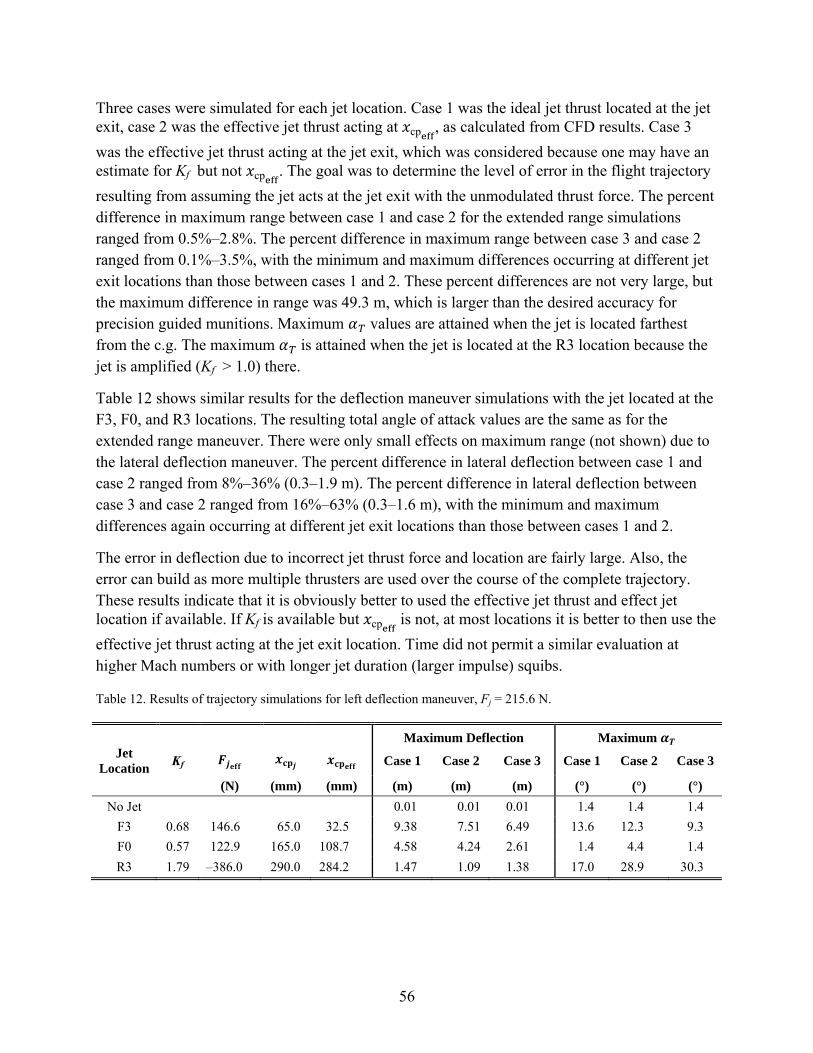
56

Three cases were simulated for each jet location. Case 1 was the ideal jet thrust located at the jet exit, case 2 was the effective jet thrust acting at cp , as calculated from CFD results. Case 3

was the effective jet thrust acting at the jet exit, which was considered because one may have an estimate for Kf but not cp . The goal was to determine the level of error in the flight trajectory

resulting from assuming the jet acts at the jet exit with the unmodulated thrust force. The percent difference in maximum range between case 1 and case 2 for the extended range simulations ranged from 0.5%–2.8%. The percent difference in maximum range between case 3 and case 2 ranged from 0.1%–3.5%, with the minimum and maximum differences occurring at different jet exit locations than those between cases 1 and 2. These percent differences are not very large, but the maximum difference in range was 49.3 m, which is larger than the desired accuracy for precision guided munitions. Maximum values are attained when the jet is located farthest from the c.g. The maximum is attained when the jet is located at the R3 location because the jet is amplified (Kf > 1.0) there.

Table 12 shows similar results for the deflection maneuver simulations with the jet located at the F3, F0, and R3 locations. The resulting total angle of attack values are the same as for the extended range maneuver. There were only small effects on maximum range (not shown) due to the lateral deflection maneuver. The percent difference in lateral deflection between case 1 and case 2 ranged from 8%–36% (0.3–1.9 m). The percent difference in lateral deflection between case 3 and case 2 ranged from 16%–63% (0.3–1.6 m), with the minimum and maximum differences again occurring at different jet exit locations than those between cases 1 and 2.

The error in deflection due to incorrect jet thrust force and location are fairly large. Also, the error can build as more multiple thrusters are used over the course of the complete trajectory. These results indicate that it is obviously better to used the effective jet thrust and effect jet location if available. If Kf is available but cp is not, at most locations it is better to then use the

effective jet thrust acting at the jet exit location. Time did not permit a similar evaluation at higher Mach numbers or with longer jet duration (larger impulse) squibs.

Table 12. Results of trajectory simulations for left deflection maneuver, Fj = 215.6 N.

Maximum Deflection Maximum Jet

Location Kf Case 1 Case 2 Case 3 Case 1 Case 2 Case 3

(N) (mm) (mm) (m) (m) (m) (°) (°) (°)

No Jet 0.01 0.01 0.01 1.4 1.4 1.4

F3 0.68 146.6 65.0 32.5 9.38 7.51 6.49 13.6 12.3 9.3

F0 0.57 122.9 165.0 108.7 4.58 4.24 2.61 1.4 4.4 1.4

R3 1.79 –386.0 290.0 284.2 1.47 1.09 1.38 17.0 28.9 30.3

57

Figure 39a shows the flight trajectory for the extended range simulation with the jet at the F3 location. The three jet cases and the ballistic case are shown. The ideal jet (case 1) overpredicts the maximum range that would be attained using the effective jet (case 2). At this location, there is a small difference between case 3 and case 2. Figure 39b shows the total angle of attack for these cases. Note that the second squib fires while the projectile body is at an angle of attack of about 6–8. The effective jet thrust and cp values could have been adjusted for the second

squib to account for this angle. Alternatively, another solution is for the second squib to be timed to occur when is near zero. In addition, Corriveau et al. (36, 37) proposed using appropriately timed pairs of thrusters to minimize the oscillations (as seen in figure 39b) induced by the firing of the first thruster. This maximized the induced deflection, while minimizing the drag induced by the oscillations and their resultant high angles of attack.

Figure 40 shows the lateral deflection predicted for the deflection maneuver with the jet located at the F3 (figure 40a) and the R3 (figure 40b) jet exit locations. When the jet is located at the F3 location, the case 1 simulation again overpredicts the deflection and the case 3 simulation underpredicts the deflection, but by less of a margin. When the jet is located at the R3 location, both the case 1 and 3 simulations overpredict the deflection, but the maximum deflection is about an order of magnitude less than when the jet is located at the F3 location. Figure 40c shows the total angle of attack for the cases when the jet is located at the R3 location. The maximum angles are about two times those for when the jet is located at the F3 location (figure 40b).

The results shown in tables 11 and 12 demonstrate that the largest control maneuver is attained when the jet is located at the nose of the projectile. Fresconi and Plostins (33) showed that the aft end of a spin-stabilized projectile is the optimum location for control actuators. A similar analysis shows that the optimum location for a control actuator on a fin-stabilized projectile is the front section of the projectile. In practical situations the designer may be limited to where the jet can be located due to other considerations for payload, GN&C components, etc. However, locating the jet near the projectile base can have the advantage of minimizing the error in the effective jet location, but the maneuver control authority will not be the optimum.

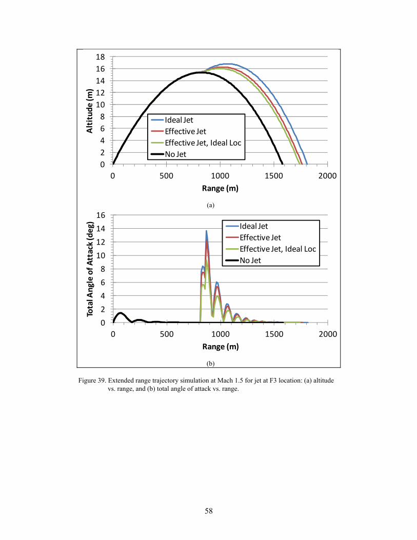
58

Figure 39. Extended range trajectory simulation at Mach 1.5 for jet at F3 location: (a) altitude vs. range, and (b) total angle of attack vs. range.

(a)

(b)

0

2

4

6

8

10

12

14

16

18

0 500 1000 1500 2000

Altitude (m

)

Range (m)

Ideal Jet

Effective Jet

Effective Jet, Ideal Loc

No Jet

0

2

4

6

8

10

12

14

16

0 500 1000 1500 2000

Total A

ngle of Attack (deg)

Range (m)

Ideal Jet

Effective Jet


No Jet

59

Figure 40. Left deflection trajectory simulation at Mach 1.5: deflection vs. range for jet at (a) F3 location, (b) R3 location, and (c) total angle of attack vs. range for jet at R3 location.

(a)

(b)

(c)

0.0

2.0

4.0

6.0

8.0

10.0

0 500 1000 1500 2000

Deflection (m

)

Range (m)

Ideal Jet

Effective Jet


‐0.2

0.0

0.2

0.4

0.6

0.8

1.0

1.2

1.4

1.6

0 500 1000 1500 2000

Deflection (m

)

Range (m)

Ideal Jet

Effective Jet


0

5

10

15

20

25

30

35

0 500 1000 1500 2000

Total A

ngle of Attack (deg)

Range (m)

Ideal Jet

Effective Jet


No Jet

60

4. Summary and Conclusions

The jet interaction effects resulting from a supersonic jet venting into a supersonic crossflow were investigated for the case of a flat plate and a generic fin-stabilized projectile. Mesh generation and turbulence model variation studies were performed with the flat plate configuration. Simulations were performed with a sonic nozzle (AR = 1) and supersonic nozzles with AR = 2 and AR = 8. Simulations were performed at three supersonic freestream Mach numbers and several jet total-to-freestream static PRs. Some conclusions that can be drawn from these flat plate results are as follows.

• The JI, as determined from the jet amplification factor, , was most dependent on PR and

the freestream Mach number.

• was found to increase with Mach number and decrease with increasing PR.

• There was only a small variation of with AR.

• There was very little variation of with the jet gas total temperature, .

• There was a strong decrease in with increasing altitude, primarily due to the increase in

PR as the freestream static pressure decreases with altitude.

• The data show that the jet force is usually amplified ( > 1) for jets issuing from a flat plate, into a supersonic freestream. decreases as the Mach number is reduced, eventually

leading to attenuation of the jet force.

For the ANF projectile, simulations were performed with a sonic nozzle located on the top surface of the projectile, at seven positions along the projectile axis. Some conclusions drawn from the ANF results are as follows.

• Locating the jet near the tail fins can minimize the traditional JI effects due to interactions in the jet wake (a well-known conclusion); however, the interaction of the near-jet flowfield with the fins must be taken into account. There is generally an amplification of the jet force when the jet is located very near the tail fins.

• The jet thrust force was attenuated 10%–23% at Mach 3.5, 16%–45% at Mach 2.5, and 26%–74% at Mach 1.5 for the forward five jet locations. The jet thrust force was amplified by 60%–102% at Mach 3.5, 70%–82% at Mach 2.5, and 5%–78% at Mach 1.5 for the two rear locations.

• In general, the moment due to the jet thrust was near neutral or amplified at most jet locations. However, at the R1 location, the moment amplification factor was negative at

61

both Mach numbers, indicating an induced moment that acts to oppose the moment due to the jet thrust.

• In all cases, the effective location of the resultant jet thrust ( cp when = 0°, cp at

all ) was either forward of the jet location or very close to it, e.g., when the jet was located near the tail.

• At the R1 location a negative (nose down) resultant pitching moment is observed, even though the jet is located to the rear of the c.g.

• For the jet located at the c.g. (F0 location), the resultant pitching moment is not zero due to the JI force, but one that induces a negative (nose down) pitching moments.

• Comparisons of the ANF results with those from a body-alone (no tail fins) configuration show that the jet flow interaction with the tail are minimal when the jet is located toward the nose of the projectile.

• At the forward four locations, more attenuation (decreasing ) of the jet force is observed

as PR decreases, which is opposite that found for the flat plate. At the rearward locations, the trend is the same as that for the flat plate, including a general amplification of the jet force.

• The jet AR was found to have a small effect on at the forward locations. At the R3 location, there was a small decreasing trend of with increasing AR.

• Flowfield visualizations of the cases with –10 ≤ ≤ 10 showed that the CVP generated by the jet plume was pushed very close to the tail fins at the high-negative angle of attack when the jet exit was located forward of the tail fins. At high-positive angles of attack, the CVP moved away from the body relatively quickly.

• These qualitative observations at ≠ 0° are consistent with the data for Kf showing that there was more variation as became more negative. The effective jet location, cp ,

varied little for > –5 at Mach 2.5 and 3.5.

• Flight trajectory simulations using reaction jet “squibs” indicated that more accurate results were obtained if the effective jet thrust and effective jet location were used rather than the values for the ideal jet thrust acting at the jet nozzle exit location.

• Reasonable results could be obtained if the effective jet thrust was used at the ideal jet location (jet nozzle exit) for the case where an estimate for cp is unknown.

Some general conclusions are:

• The features of the jet interaction flowfield compared well with those presented and described in the archival literature.

62

• The choice of turbulence model can affect accurate prediction of the features of the interaction flowfield. In the flat plate configuration, differences of up to 13% and 15% were observed in the force amplification factor and JI force, respectively.

These results confirm that the choice of location for a reaction jet can have a significant effect on the resulting aerodynamic forces and moments. Additional work is planned to further analyze the data generated thusfar to determine if correlations exist to enable predicting the Kf and cp

values. Work is also planned to investigate transient effects of a pulsed jet, with and without projectile roll, to determine if the JI predicted from steady-state simulations are the same in unsteady flowfields.

63

5. References

1. Margason, R. J. Fifty Years of Jet in Cross Flow Research. AGARD, 72nd Fluid Dynamics Panel Meeting, (1), 1993.

2. Spaid, F. W.; Cassel, L. A. Aerodynamics Interference Induced by Reaction Controls. AGARDograph (173), December 1973.

3. Champigny, P.; Lacau, R. G. Lateral Jet Control for Tactical Missiles. Special Course on Missile Aerodynamics; AGARD-R-804 (3), 1994.

4. Cassel, L. A. Applying Jet Interaction Technology. AIAA Journal of Spacecraft and Rockets July/August 2003, 40 (4), 523–537.

5. Dickmann, D. A.; Lu, F. K. Shock/Boundary-Layer Interaction Effects on Transverse Jets in Crossflow Over a Flat Plate. AIAA Journal of Spacecraft and Rockets November/December 2009, 46 (6), 1132–1141.

6. Dickmann, D. A.; Lu, F. K. Shock/Boundary Layer Interaction Effects of Transverse Jets in Crossflow Over a Body of Revolution; AIAA-2009-4146. Presented at the 19th AIAA Computational Fluid Dynamics Conference, San Antonio, TX, June 2009.

7. Kovar, A.; Schulein, E. Comparison of Experimental and Numerical Investigation on a Jet in a Supersonic Cross-Flow. The Aeronautical Journal June 2006, 353–360.

8. Stahl, B.; Esch, H.; Gulhan, A. Experimental investigation of Side Jet Interaction With a Supersonic Cross Flow. Aerospace Science and Technology 2008, 12 (4), 269–275.

9. Stahl, B.; Edmunds, H.; Gulhan, A. Experimental Investigation of Hot and Cold Side Jet Interaction With a Supersonic Cross Flow. Aerospace Science and Technology 2009, 13, (8), 488–496.

10. Stahl, B.; Siebe, F.; Gulhan, A. Hot-Gas Side Jet in a Supersonic Freestream. AIAA Journal of Spacecraft and Rockets November/December 2010, 47 (6), 957–965.

11. Gnemmi, P.; Adeli, R.; Longo, J. Computational Comparisons of the Interaction of a Lateral Jet on a Supersonic Generic Missile; AIAA-2008-6883. Presented at the AIAA Atmospheric Flight Mechanics Conference, Honolulu, HI, August 2008.

12. Gnemmi, P.; Schafer, H. J. Experimental and Numerical Investigations of a Transverse Jet Interaction on a Missile Body; AIAA-2005-0052. Presented at the 43rd AIAA Aerospace Sciences Meeting and Exhibit, Reno, NV, January 2005.

64

13. Graham, M. J.; Weinacht, P. Numerical Investigation of Supersonic Jet Interaction for Axisymmetric Bodies. AIAA Journal of Spacecraft and Rockets Sept/Oct 2000, 37 (5), 675–683.

14. Graham, M. J.; Weinacht, P.; Brandeis, J. Numerical Investigation of Supersonic Jet Interaction for Finned Bodies. AIAA Journal of Spacecraft and Rockets May/June 2002, 39 (3), 376–383.

15. Beresh, S. J.; Henfling, J. F.; Erven, R. J.; Spillers, R. W. Penetration of a Transverse Supersonic Jet into a Subsonic Compressible Crossflow. AIAA Journal Feb 2005, 43 (2), 379–389.

16. Beresh, S. J.; Henfling, J. F.; Erven, R. J.; Spillers, R. W. Turbulent Characteristics of a Transverse Supersonic Jet Into a Subsonic Compressible Crossflow. AIAA Journal Nov 2005, 43 (11), 2385–2394.

17. Beresh, S. J.; Henfling, J. F.; Erven, R. J.; Spillers, R. W. Crossplane Velocimetry of a Transverse Supersonic Jet in a Transonic Crossflow. AIAA Journal Dec 2006, 44 (12), 3051–3061.

18. Beresh, S. J.; Heineck, J. T.; Walker, S. M.; Schairer, E. T.; Yaste, D. M., Stereoscopic PIV for Jet/Fin Interaction Measurements on a Full-Scale Flight Vehicle; AIAA-2005-0442. Presented at the 43rd AIAA Aerospace Sciences Meeting and Exhibit, Reno, NV, Jan 2005.

19. Beresh, S. J. Aerodynamic Origin of Jet/Fin Interaction on a Full-Scale Flight Vehicle Configuration; AIAA-2007-0673. Presented at the 45th AIAA Aerospace Sciences Meeting and Exhibit, Reno, NV, Jan 2007.

20. Dowdy, M. W.; Newton, J. F. Investigation of Liquid and Gaseous Secondary Injection Phenomena on a Flat Plate With M = 2.01 and M = 4.54; JPL-TR-32-542; Dec 1963.

21. Metacomp Technologies, Inc. MIME User Manual, Agoura Hills, CA, 2008.

22. Dupuis, A. D., “Aeroballistic Range and Wind Tunnel Tests of the Basic Finner Reference Projectile from Subsonic to High Supersonic Velocities,” TM-2002-137, Defence R&D Canada Valcartier, Canada, Oct 2002.

23. Dupuis, A. D.; Hathaway, W. Aeroballistic Range Tests of the Basic Finner Reference Projectile at Supersonic Velocities; DREV-TM-9703; Defence Research Establishment, Valcartier, Canada, Aug 1997.

24. Metacomp Technologies, Inc., “CFD ++ User Manual,” Agoura Hills, CA, 2010.

25. Menter, F. R. Two-Equation Eddy-Viscosity Turbulence Models For Engineering Applications. AIAA Journal Aug 1994, 32 (8), 1598–1605.

65

26. Hirsch, C. Lessons Learned From the First AIAA-SWBLI. Workshop CFD Simulations of Two Test Cases; AIAA-2010-4824. Presented at the 28th AIAA Applied Aerodynamics Conference, Chicago, IL, June 2010.

27. Spalart, P. R.; Allmaras, S. R. A One-Equation Turbulence Model for Aerodynamic Flows. Recherche Aerospatiale 1994, (1), 5–21.

28. Chien, K. -Y. Predictions of Channel and Boundary Layer Flows with a Low-Reynolds-Number Turbulence Model. AIAA Journal Jan 1982, 20 (1), 33–38.

29. Goldberg, U.; Batten, P.; Palaniswamy, S.; Chakravarthy, S.; Peroomian, O. Hypersonic Flow Predictions Using Linear and Nonlinear Turbulence Closures. AIAA Journal of Aircraft July/Aug 2000, 37 (4), 671–675.

30. Goldberg, U.; Peroomian, O.; Chakravarthy, S. Application of the k-ε-R Turbulence Model to Wall-Bounded Compressive Flows; AIAA 98-0323. Presented at the 36th AIAA Aerospace Sciences Meeting and Exhibit, Reno, NV, Jan 1998.

31. Batten, P.; Craft, T. J.; Leschziner, M. A.; Loyau, H. Reynolds-Stress-Transport Modeling for Compressible Aerodynamics Applications. AIAA Journal July 1999, 37 (7), 785–797.

32. DeSpirito, J. Turbulence Model Effects on Cold-Gas Lateral Jet Interaction in a Supersonic Crossflow; ARL Report in Preparation; U.S. Army Research Laboratory: Aberdeen Proving Ground, MD.

33. Fresconi, F.; Plostins, P. Control Mechanism Strategies for Spin-Stabilized Projectiles. J. Aerospace Engineering 2010, 224 (G9), 979–991.

34. Ollerenshaw, D.; Costello, M. Simplified Projectile Swerve Solution for General Control Inputs. AIAA Journal of Guidance, Control, and Dynamics Sept/Oct 2008, 31 (5), 1259–1265.

35. Arrow Tech Associates, 1233 Shelburne Rd., Ste D8, South Burlington, VT 05403.

36. Corriveau, D.; Wey, P.; Berner, C. Analytical Model Development and Impulse Thrusters Pairing Guidelines for Trajectory Corrections of Spin-Stabilized Projectiles; AIAA-2010-0665. Presented at the 48th AIAA Aerospace Sciences Meeting and Exhibit, Orlando, FL, Jan 2010.

37. Corriveau, D.; Wey, P.; Berner, C. Thrusters Pairing Guidelines for Trajectory Corrections of Projectiles. AIAA Journal of Guidance, Control, and Dynamics July/Aug 2011, 34 (4), 1120–1128.

66

INTENTIONALLY LEFT BLANK.

67

Appendix A. Army-Navy Finner With No Jet Validation

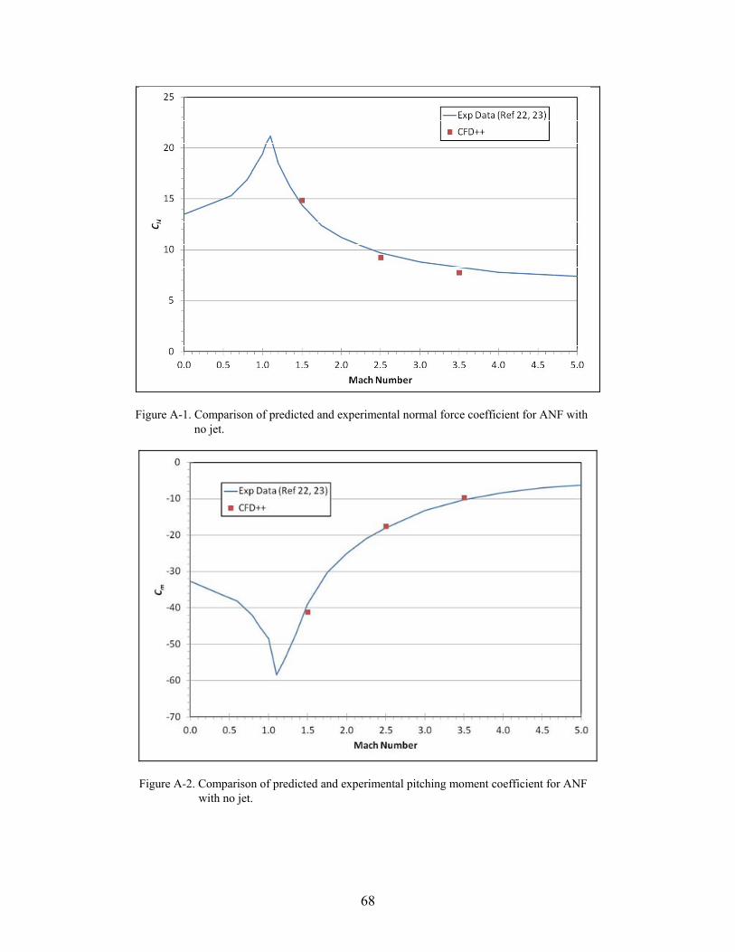
68

Figure A-1. Comparison of predicted and experimental normal force coefficient for ANF with no jet.

Figure A-2. Comparison of predicted and experimental pitching moment coefficient for ANF with no jet.

69

Appendix B. Army-Navy Finner Tabulated Results at = 0°

70

Table B-1. Amplification factor, normal force, and pitching moment results as function of jet location on ANF body-tail configuration (M = 1.5, PR = 340, AR = 1, = 0°).

Jet Loc Jet Loc Kf Km total

total

(m)

F3 0.0650 0.67 0.91 –1.9131 0.6219 –1.3027 –6.3675 0.5519 –5.7550

F2 0.0900 0.74 1.06 –1.9120 0.4895 –1.4341 –4.7796 –0.2771 –4.9960

F1 0.1275 0.68 1.40 –1.9116 0.6167 –1.3065 –2.3891 –0.9502 –3.2785

F0 0.1650 0.57 –1.9118 0.8248 –1.0986 0.0004 –2.1226 –2.0615

R1 0.2150 0.26 –0.68 –1.9118 1.4172 –0.5062 3.1868 –5.3588 –2.1113

R2 0.2650 1.05 0.98 –1.9118 –0.1047 –2.0281 6.3728 –0.1217 6.3119

R3 0.2900 1.78 1.70 –1.9118 –1.4955 –3.4189 7.9664 5.5523 13.5793

Table B-2. Center of pressure results as function of jet location on ANF body-tail configuration (M = 1.5, PR = 340, AR = 1, = 0°).

Jet Loc Jet Loc cp cptotal cp cpeff

cp cptotal cp cpeff

(m) (cal.) (cal.) (cal.) (cal.) (mm) (mm) (mm) (mm)

F3 0.0650 –3.33 –4.42 –0.89 –4.50 –99.9 –132.5 –26.6 –135.1

F2 0.0900 –2.50 –3.48 0.57 –3.55 –75.0 –104.5 17.0 –106.6

F1 0.1275 –1.25 –2.51 1.54 –2.58 –37.5 –75.3 46.2 –77.4

F0 0.1650 0.00 –1.88 2.57 –1.95 0.0 –56.3 77.2 –58.6

R1 0.2150 1.67 –4.17 3.78 –4.39 50.0 –125.1 113.4 –131.7

R2 0.2650 3.33 3.11 –1.16 3.10 100.0 93.4 –34.8 93.0

R3 0.2900 4.17 3.97 3.71 3.97 125.0 119.2 111.4 119.0



total

(m)

F3 0.0650 0.73 0.99 –0.6894 0.1871 –0.5049 –2.2946 0.0149 –2.2348

F2 0.0900 0.84 1.15 –0.6884 0.1134 –0.5775 –1.7208 –0.2606 –1.9365

F1 0.1275 0.72 1.54 –0.6881 0.1957 –0.4950 –0.8600 –0.4673 –1.2824

F0 0.1650 0.69 –0.6882 0.2123 –0.4785 0.0002 –0.6711 –0.6260

R1 0.2150 0.55 –0.15 –0.6882 0.3076 –0.3832 1.1471 –1.3160 –0.1240

R2 0.2650 1.70 1.65 –0.6882 –0.4821 –1.1729 2.2940 1.6527 3.9916

R3 0.2900 1.82 1.77 –0.6882 –0.5610 –1.2518 2.8675 2.2180 5.1303

71



cp cptotal cp cpeff


F3 0.0650 –3.33 –4.43 –0.08 –4.54 –99.9 –132.8 –2.4 –136.2

F2 0.0900 –2.50 –3.35 2.30 –3.45 –75.0 –100.6 68.9 –103.4

F1 0.1275 –1.25 –2.59 2.39 –2.70 –37.5 –77.7 71.6 –80.9

F0 0.1650 0.00 –1.31 3.16 –1.41 0.0 –39.3 94.8 –42.3

R1 0.2150 1.67 –0.32 4.28 –0.44 50.0 –9.7 128.4 –13.3

R2 0.2650 3.33 3.40 3.43 3.37 100.0 102.1 102.8 101.2

R3 0.2900 4.17 4.10 3.95 4.07 125.0 123.0 118.6 122.1



total

— (m) — — — — — — — —

F3 0.0650 0.77 1.10 –0.3517 0.0815 –0.2704 –1.1708 –0.1218 –1.2921

F2 0.0900 0.90 1.25 –0.3512 0.0349 –0.3165 –0.8780 –0.2159 –1.0934

F1 0.1275 0.83 1.54 –0.3511 0.0605 –0.2908 –0.4388 –0.2377 –0.6762

F0 0.1650 0.87 — –0.3511 0.0452 –0.3060 0.0001 –0.2040 –0.2035

R1 0.2150 0.87 0.53 –0.3512 0.0455 –0.3058 0.5853 –0.2723 0.3134

R2 0.2650 2.02 2.15 –0.3511 -0.3582 –0.7095 1.1706 1.3425 2.5135

R3 0.2900 1.60 1.57 –0.3511 -0.2118 –0.5631 1.4631 0.8371 2.3006



cp cptotal cp cpeff


F3 0.0650 –3.33 –4.78 1.49 –4.78 –99.9 –143.4 44.8 –143.5

F2 0.0900 –2.50 –3.46 6.19 –3.46 –75.0 –103.7 185.6 –103.7

F1 0.1275 –1.25 –2.33 3.93 –2.33 –37.5 –69.8 118.0 –69.8

F0 0.1650 0.00 –0.67 4.51 –0.67 0.0 –20.0 135.3 –20.0

R1 0.2150 1.67 1.02 5.99 1.02 50.0 30.7 179.6 30.7

R2 0.2650 3.33 3.54 3.75 3.54 100.0 106.3 112.4 106.3

R3 0.2900 4.17 4.09 3.95 4.09 125.0 122.6 118.5 122.6

72

Table B-7. Amplification factor, normal force, and pitching moment results as function of jet location on ANF body-alone configuration (M = 1.5, PR = 340, AR = 1, = 0°).


total

(m)

F3 0.0650 0.79 0.78 –1.9131 0.4022 –1.5113 –6.3654 1.4244 –4.9408

F2 0.0900 0.86 0.86 –1.9114 0.2637 –1.6481 –4.7791 0.6638 –4.1150

F1 0.1275 0.85 0.86 –1.9117 0.2961 –1.6161 –2.3893 0.3450 –2.0440

F0 0.1650 0.82 –1.9111 0.3465 –1.5650 –0.0004 –0.2565 –0.2566

R1 0.2150 0.72 0.43 –1.9114 0.5388 –1.3730 3.1849 –1.8163 1.3689

R2 0.2650 0.88 0.81 –1.9111 0.2215 –1.6900 6.3694 –1.2132 5.1565

R3 0.2900 1.11 1.09 –1.9119 -0.2089 –2.1212 7.9667 0.6862 8.6531

Table B-8. Amplification factor, normal force, and pitching moment results as function of jet location on ANF body-alone configuration (M = 2.5, PR = 340, AR = 1, = 0°).


total

(m)

F3 0.0650 0.85 0.83 –0.6893 0.1031 –0.5866 –2.2936 0.3843 –1.9090

F2 0.0900 0.95 0.94 –0.6881 0.0319 –0.6566 –1.7205 0.0985 –1.6217

F1 0.1275 0.86 1.03 –0.6882 0.0947 –0.5939 –0.8601 –0.0277 –0.8876

F0 0.1650 0.81 –0.6879 0.1297 –0.5587 –0.0001 –0.2779 –0.2778

R1 0.2150 0.76 0.41 –0.6880 0.1630 –0.5254 1.1465 –0.6783 0.4685

R2 0.2650 0.98 0.91 –0.6879 0.0158 –0.6725 2.2927 –0.2111 2.0818

R3 0.2900 1.18 1.16 –0.6882 –0.1245 –0.8131 2.8676 0.4659 3.3337



total

(m)

F3 0.0650 0.57 0.86 –0.8262 0.3536 –0.4730 –2.7499 0.3754 –2.3742

F2 0.0900 0.69 1.07 –0.8250 0.2547 –0.5707 –2.0621 –0.1532 –2.2150

F1 0.1275 0.56 1.54 –0.8247 0.3639 –0.4612 –1.0307 –0.5592 –1.5896

F0 0.1650 0.53 –0.8248 0.3883 –0.4369 0.0003 –0.8957 –0.8951

R1 0.2150 0.30 –0.48 –0.8249 0.5752 –0.2501 1.3751 –2.0285 –0.6532

R2 0.2650 1.08 0.95 –0.8249 –0.0684 –0.8937 2.7499 –0.1502 2.6000

R3 0.2900 2.21 2.11 –0.8250 –0.9971 –1.8225 3.4377 3.8125 7.2505

73


Jet Loc Jet Loc cp cptotal cp cp cptotal

cp

(m) (cal.) (cal.) (cal.) (mm) (mm) (mm)

F3 0.0650 –3.33 –5.020 –1.062 –99.9 –150.6 –31.8

F2 0.0900 –2.50 –3.881 0.601 –75.0 –116.4 18.0

F1 0.1275 –1.25 –3.446 1.537 –37.5 –103.4 46.1

F0 0.1650 0.00 –2.049 2.306 0.0 –61.5 69.2

R1 0.2150 1.67 –2.612 3.527 50.0 –78.3 105.8

R2 0.2650 3.33 2.909 –2.198 100.0 87.3 –65.9

R3 0.2900 4.17 3.978 3.823 125.0 119.3 114.7



total

(m)

F3 0.0650 0.65 0.99 –0.2980 0.1050 –0.1934 –0.9918 0.0092 –0.9824

F2 0.0900 0.81 1.15 –0.2970 0.0552 –0.2423 –0.7424 –0.1089 –0.8511

F1 0.1275 0.62 1.70 –0.2969 0.1124 –0.1849 –0.3710 –0.2583 –0.6290

F0 0.1650 0.61 –0.2969 0.1171 –0.1803 0.0001 –0.3737 –0.3733

R1 0.2150 0.64 0.08 –0.2969 0.1059 –0.1915 0.4950 –0.4553 0.0399

R2 0.2650 2.02 1.09 –0.2969 –0.3036 –0.6009 0.9899 1.0906 2.0808

R3 0.2900 1.83 1.80 –0.2970 –0.2450 –0.5424 1.2374 0.9856 2.2232



cp


F3 0.0650 –3.33 –5.079 –0.087 –99.9 –152.4 –2.6

F2 0.0900 –2.50 –3.513 1.975 –75.0 –105.4 59.3

F1 0.1275 –1.25 –3.402 2.298 –37.5 –102.1 68.9

F0 0.1650 0.00 –2.071 3.192 0.0 –62.1 95.8

R1 0.2150 1.67 0.208 4.301 50.0 6.3 129.0

R2 0.2650 3.33 3.463 3.593 100.0 103.9 107.8

R3 0.2900 4.17 4.099 4.022 125.0 123.0 120.7

74



total

(m)

F3 0.0650 0.38 0.86 –0.2713 0.1671 –0.1046 –0.9030 0.1242 –0.7785

F2 0.0900 0.56 1.21 –0.2699 0.1196 –0.1508 –0.6749 –0.1431 –0.8177

F1 0.1275 0.40 1.91 –0.2698 0.1614 –0.1088 –0.3372 –0.3064 –0.6433

F0 0.1650 0.38 –0.2698 0.1678 –0.1024 0.0000 –0.4345 –0.4342

R1 0.2150 0.25 –0.60 –0.2698 0.2020 –0.0682 0.4497 –0.7191 –0.2691

R2 0.2650 1.38 1.24 –0.2699 –0.1036 –0.3740 0.8997 0.2170 1.1169

R3 0.2900 2.80 2.71 –0.2700 –0.4855 –0.7559 1.1249 1.9216 3.0467



cp


F3 0.0650 –3.33 –7.440 –0.744 –99.9 –223.2 –22.3

F2 0.0900 –2.50 –5.424 1.196 –75.0 –162.7 35.9

F1 0.1275 –1.25 –5.912 1.898 –37.5 –177.3 56.9

F0 0.1650 0.00 –4.241 2.589 0.0 –127.2 77.7

R1 0.2150 1.67 –3.945 3.559 50.0 –118.3 106.8

R2 0.2650 3.33 2.987 2.094 100.0 89.6 62.8

R3 0.2900 4.17 4.031 3.958 125.0 120.9 118.7



total

(m)

F3 0.0650 0.58 1.03 –0.0977 0.0409 –0.0573 –0.3254 –0.0089 –0.3340

F2 0.0900 0.75 1.27 –0.0972 0.0243 –0.0732 –0.2429 –0.0662 –0.3088

F1 0.1275 0.46 2.23 –0.0971 0.0524 –0.0451 –0.1214 –0.1495 –0.2706

F0 0.1650 0.56 –0.0971 0.0431 –0.0544 0.0000 –0.1590 –0.1588

R1 0.2150 0.76 0.23 –0.0971 0.0236 –0.0739 0.1619 –0.1253 0.0368

R2 0.2650 2.36 0.49 –0.0972 –0.1324 –0.2300 0.3239 0.4943 0.8185

R3 0.2900 1.81 1.79 –0.0972 –0.0783 –0.1759 0.4050 0.3182 0.7234

75



cp


F3 0.0650 –3.33 –5.831 0.218 –99.9 –174.9 6.5

F2 0.0900 –2.50 –4.217 2.719 –75.0 –126.5 81.6

F1 0.1275 –1.25 –6.002 2.850 –37.5 –180.1 85.5

F0 0.1650 0.00 –2.917 3.690 0.0 –87.5 110.7

R1 0.2150 1.67 0.498 5.311 50.0 14.9 159.3

R2 0.2650 3.33 3.559 3.734 100.0 106.8 112.0

R3 0.2900 4.17 4.113 4.065 125.0 123.4 122.0



total

(m)

F3 0.0650

F2 0.0900

F1 0.1275 0.75 1.42 –0.7761 0.1969 –0.5795 –0.9698 –0.4098 –1.3793

F0 0.1650 0.72 –0.7758 0.2135 –0.5628 0.0004 –0.6208 –0.6202

R1 0.2150

R2 0.2650

R3 0.2900 1.62 1.60 –0.7759 –0.4787 –1.2550 3.2331 1.9363 5.1696



cp


F3 0.0650

F2 0.0900

F1 0.1275 –1.25 –2.380 2.081 –37.5 –71.4 62.4

F0 0.1650 0.00 –1.102 2.908 0.0 –33.1 87.3

R1 0.2150

R2 0.2650

R3 0.2900 4.17 4.119 4.045 125.0 123.6 121.3

76



total

(m)

F3 0.0650

F2 0.0900

F1 0.1275 0.66 1.61 –0.3337 0.1137 –0.2205 –0.4170 –0.2558 –0.6726

F0 0.1650 0.65 –0.3336 0.1174 –0.2166 0.0001 –0.3609 –0.3605

R1 0.2150

R2 0.2650

R3 0.2900 1.60 1.58 –0.3338 –0.1995 –0.5337 1.3908 0.8096 2.2007



cp


F3 0.0650

F2 0.0900

F1 0.1275 –1.25 –3.051 2.251 –37.5 –91.5 67.5

F0 0.1650 0.00 –1.664 3.073 0.0 –49.9 92.2

R1 0.2150

R2 0.2650

R3 0.2900 4.17 4.123 4.058 125.0 123.7 121.7



total

(m)

F3 0.0650

F2 0.0900

F1 0.1275 0.49 2.10 –0.1079 0.0549 –0.0535 –0.1349 –0.1482 –0.2828

F0 0.1650 0.58 –0.1080 0.0458 –0.0627 0.0000 –0.1597 –0.1594

R1 0.2150

R2 0.2650

R3 0.2900 1.59 1.58 –0.1082 –0.0636 –0.1722 0.4507 0.2598 0.7108

77



cp


F3 0.0650

F2 0.0900

F1 0.1275 –1.25 –5.291 2.700 –37.5 –158.7 81.0

F0 0.1650 0.00 –2.544 3.490 0.0 –76.3 104.7

R1 0.2150

R2 0.2650

R3 0.2900 4.17 4.127 4.083 125.0 123.8 122.5



total

(m)

F3 0.0650

F2 0.0900

F1 0.1275 0.77 1.41 –0.8615 0.1999 –0.6620 –1.0769 –0.4441 –1.5207

F0 0.1650 0.75 –0.8618 0.2149 –0.6474 –0.0003 –0.6555 –0.6555

R1 0.2150

R2 0.2650

R3 0.2900 1.40 1.39 –0.8619 –0.3481 –1.2104 3.5910 1.4066 4.9979



cp


F3 0.0650

F2 0.0900

F1 0.1275 –1.25 –2.297 2.222 –37.5 –68.9 66.7

F0 0.1650 0.00 –1.013 3.051 0.0 –30.4 91.5

R1 0.2150

R2 0.2650

R3 0.2900 4.17 4.129 4.041 125.0 123.9 121.2

78



total

(m)

F3 0.0650

F2 0.0900

F1 0.1275 0.68 1.56 –0.3660 0.1172 –0.2492 –0.4575 –0.2555 –0.7127

F0 0.1650 0.69 –0.3661 0.1137 –0.2528 –0.0002 –0.3336 –0.3335

R1 0.2150

R2 0.2650

R3 0.2900 1.39 1.38 –0.3663 –0.1424 –0.5092 1.5260 0.5744 2.1007



cp


F3 0.0650

F2 0.0900

F1 0.1275 –1.25 –2.860 2.180 –37.5 –85.8 65.4

F0 0.1650 0.00 –1.319 2.933 0.0 –39.6 88.0

R1 0.2150

R2 0.2650

R3 0.2900 4.17 4.126 4.032 125.0 123.8 121.0

79



total

(m)

F3 0.0650

F2 0.0900

F1 0.1275 0.47 2.07 –0.1140 0.0603 –0.0541 –0.1437 –0.1530 –0.2964

F0 0.1650 0.57 –0.1143 0.0489 –0.0658 –0.0015 –0.1599 –0.1612

R1 0.2150

R2 0.2650

R3 0.2900 1.40 1.40 –0.1149 –0.0465 –0.1618 0.4769 0.1890 0.6662



cp


F3 0.0650

F2 0.0900

F1 0.1275 –1.25 –5.482 2.537 –37.8 –164.5 76.1

F0 0.1650 0.00 –2.451 3.270 –0.4 –73.5 98.1

R1 0.2150

R2 0.2650

R3 0.2900 4.17 4.117 4.063 124.6 123.5 121.9

80


81

Appendix C. Army-Navy Finner Tabulated Results at = ±10°

82

Table C-1. Amplification factor, normal force, and pitching moment results as function of jet location on ANF body-tail configuration (M = 1.5, PR = 340, AR = 1, = –10°).


total

(m)

F3 0.0650 0.33 1.37 –1.9131 1.2766 –3.3380 –6.3674 –2.3359 –1.7209

F2 0.0900 0.51 1.58 –1.9120 0.9334 –3.6802 –4.7796 –2.7565 –0.5537

F1 0.1275 0.42 2.38 –1.9116 1.1113 –3.5018 –2.3891 –3.2913 1.3020

F0 0.1650 0.41 0.00 –1.9118 1.1372 –3.4761 0.0004 –3.6991 3.2837

R1 0.2150 0.06 –1.15 –1.9118 1.7975 –2.8159 3.1868 –6.8418 3.3274

R2 0.2650 0.64 0.49 –1.9118 0.6873 –3.9260 6.3729 –3.2641 10.0911

R3 0.2900 1.54 1.48 –1.9119 –1.0375 –5.6510 7.9668 3.8621 18.8113

Table C-2. Center of pressure results as function of jet location on ANF body-tail configuration (M = 1.5, PR = 340, AR = 1, = –10°).


cp cptotal cp cpeff


F3 0.0650 –3.33 –0.52 1.83 –13.67 –99.9 –15.5 54.9 –410.2

F2 0.0900 –2.50 –0.15 2.95 –7.70 –75.0 –4.5 88.6 –231.0

F1 0.1275 –1.25 0.37 2.96 –7.10 –37.5 11.2 88.8 –212.9

F0 0.1650 0.00 0.94 3.25 –4.78 0.0 28.3 97.6 –143.3

R1 0.2150 1.67 1.18 3.81 –31.98 50.0 35.4 114.2 –959.3

R2 0.2650 3.33 2.57 4.75 2.54 100.0 77.1 142.5 76.2

R3 0.2900 4.17 3.33 3.72 4.01 125.0 99.9 111.7 120.3

Table C-3. Amplification factor, normal force, and pitching moment results as function of jet location on ANF body-tail configuration (M = 1.5, PR = 340, AR = 1, = 10°).


total

(m)

F3 0.0650 0.65 0.73 –1.9131 0.6642 1.4527 –6.3675 1.7508 –11.5992

F2 0.0900 0.71 0.90 –1.9120 0.5506 1.3401 –4.7796 0.4945 –11.2674

F1 0.1275 0.70 1.18 –1.9116 0.5764 1.3663 –2.3891 –0.4413 –9.8128

F0 0.1650 0.69 0.00 –1.9118 0.5967 1.3865 0.0004 –0.9421 –7.9240

R1 0.2150 0.44 –0.21 –1.9118 1.0641 1.8538 3.1868 –3.8410 –7.6366

R2 0.2650 1.28 1.24 –1.9117 –0.5313 0.2586 6.3728 1.5289 0.9192

R3 0.2900 1.92 1.84 –1.9118 –1.7564 –0.9667 7.9665 6.7049 7.6889

83

Table C-4. Center of pressure results as function of jet location on ANF body-tail configuration (M = 1.5, PR = 340, AR = 1, = 10°).


cp cptotal cp cpeff


F3 0.0650 –3.33 7.98 –2.64 –3.70 –99.9 239.5 –79.1 –110.9

F2 0.0900 –2.50 8.41 –0.90 –3.15 –75.0 252.2 –26.9 –94.4

F1 0.1275 –1.25 7.18 0.77 –2.12 –37.5 215.5 23.0 –63.6

F0 0.1650 0.00 5.72 1.58 –0.72 0.0 171.5 47.4 –21.5

R1 0.2150 1.67 4.12 3.61 –0.77 50.0 123.6 108.3 –23.2

R2 0.2650 3.33 –3.56 2.88 3.23 100.0 –106.7 86.3 97.0

R3 0.2900 4.17 7.95 3.82 4.00 125.0 238.6 114.5 120.0

Table C-5. Amplification factor, normal force, and pitching moment results as function of jet location on ANF body-tail configuration (M = 2.5, PR = 340, AR = 1, = -10°).


total

(m)

F3 0.0650 0.23 1.34 –0.6898 0.5321 –2.0523 –2.2961 –0.7711 –0.0824

F2 0.0900 0.61 1.51 –0.6885 0.2662 –2.3170 –1.7212 –0.8851 0.3784

F1 0.1275 0.59 1.95 –0.6882 0.2846 –2.2982 –0.8601 –0.8138 1.3108

F0 0.1650 0.59 0.00 –0.6882 0.2789 –2.3040 0.0001 –0.9614 2.0235

R1 0.2150 0.46 –0.30 –0.6883 0.3702 –2.2127 1.1472 –1.4864 2.6456

R2 0.2650 1.56 1.54 –0.6883 –0.3829 –2.9659 2.2946 1.2430 6.5224

R3 0.2900 2.15 2.12 –0.6882 –0.7944 –3.3773 2.8676 3.2139 9.0662

Table C-6. Center of pressure results as function of jet location on ANF body-tail configuration (M = 2.5, PR = 340, AR = 1, = -10°).


cp cptotal cp cpeff


F3 0.0650 –3.33 –0.04 1.45 –19.45 –99.9 –1.2 43.5 –583.5

F2 0.0900 –2.50 0.16 3.32 –6.17 –75.0 4.9 99.7 –185.2

F1 0.1275 –1.25 0.57 2.86 –4.15 –37.5 17.1 85.8 –124.4

F0 0.1650 0.00 0.88 3.45 –2.35 0.0 26.3 103.4 –70.4

R1 0.2150 1.67 1.20 4.02 –1.07 50.0 35.9 120.5 –32.0

R2 0.2650 3.33 2.20 3.25 3.30 100.0 66.0 97.4 99.1

R3 0.2900 4.17 2.68 4.05 4.10 125.0 80.5 121.4 123.1

84



total

(m)

F3 0.0650 0.66 1.08 –0.6888 0.2349 1.4407 –2.2926 –0.1873 –5.4647

F2 0.0900 0.80 1.22 –0.6883 0.1387 1.3451 –1.7205 –0.3820 –5.0873

F1 0.1275 0.76 1.53 –0.6881 0.1631 1.3696 –0.8600 –0.4564 –4.3010

F0 0.1650 0.74 0.00 –0.6882 0.1801 1.3866 0.0002 –0.5202 –3.5048

R1 0.2150 0.68 0.29 –0.6882 0.2168 1.4232 1.1471 –0.8142 –2.6518

R2 0.2650 1.59 1.65 –0.6883 –0.4083 0.7980 2.2944 1.5001 0.8098

R3 0.2900 1.86 1.83 –0.6882 –0.5931 0.6133 2.8678 2.3704 2.2535



cp cptotal cp cpeff


F3 0.0650 –3.33 3.79 0.80 –5.46 –99.9 113.8 23.9 –163.9

F2 0.0900 –2.50 3.78 2.75 –3.83 –75.0 113.5 82.6 –114.8

F1 0.1275 –1.25 3.14 2.80 –2.51 –37.5 94.2 84.0 –75.2

F0 0.1650 0.00 2.53 2.89 –1.02 0.0 75.8 86.7 –30.7

R1 0.2150 1.67 1.86 3.76 0.71 50.0 55.9 112.7 21.2

R2 0.2650 3.33 –1.01 3.67 3.46 100.0 –30.4 110.2 103.8

R3 0.2900 4.17 –3.67 4.00 4.09 125.0 –110.2 119.9 122.6

Table C-9. Amplification factor, normal force, and pitching moment results as function of jet location on ANF body-tail configuration (M = 3.5, PR = 340, AR = 1, = –10°).


total

(m)

F3 0.0650 –0.01 1.55 –0.3523 0.3544 –1.6603 –1.1727 –0.6432 0.1519

F2 0.0900 0.51 1.71 –0.3513 0.1704 –1.8433 –0.8782 –0.6270 0.4625

F1 0.1275 0.52 2.41 –0.3511 0.1670 –1.8465 –0.4389 –0.6170 0.9119

F0 0.1650 0.54 0.00 –0.3512 0.1612 –1.8524 0.0001 –0.6967 1.2712

R1 0.2150 0.71 0.13 –0.3512 0.1022 –1.9114 0.5854 –0.5086 2.0445

R2 0.2650 2.27 2.38 –0.3512 –0.4454 –2.4590 1.1708 1.6175 4.7561

R3 0.2900 1.79 1.75 –0.3512 –0.2761 –2.2897 1.4632 1.0994 4.5304

85

Table C-10. Center of pressure results as function of jet location on ANF body-tail configuration (M = 3.5, PR = 340, AR = 1, = –10°).


cp cptotal cp cpeff


F3 0.0650 –3.33 0.09 1.81 0.00 –99.9 2.7 54.4 0.0

F2 0.0900 –2.50 0.25 3.68 –8.32 –75.0 7.5 110.4 –249.6

F1 0.1275 –1.25 0.49 3.69 –5.73 –37.5 14.8 110.8 –172.0

F0 0.1650 0.00 0.69 4.32 –3.67 0.0 20.6 129.7 –110.0

R1 0.2150 1.67 1.07 4.98 0.31 50.0 32.1 149.4 9.3

R2 0.2650 3.33 1.93 3.63 3.50 100.0 58.0 109.0 105.0

R3 0.2900 4.17 1.98 3.98 4.09 125.0 59.4 119.4 122.6



total

(m)

F3 0.0650 1.10 1.14 –0.3514 –0.0353 1.2757 –1.1696 –0.1646 –3.3020

F2 0.0900 1.15 1.20 –0.3512 –0.0537 1.2575 –0.8779 –0.1738 –3.0194

F1 0.1275 1.12 1.24 –0.3511 –0.0433 1.2680 –0.4388 –0.1050 –2.5116

F0 0.1650 1.12 0.00 –0.3511 –0.0408 1.2704 0.0001 0.0078 –1.9598

R1 0.2150 1.14 1.31 –0.3512 –0.0477 1.2635 0.5854 0.1793 –1.2031

R2 0.2650 1.55 1.63 –0.3512 –0.1944 1.1168 1.1707 0.7412 –0.0558

R3 0.2900 1.89 1.88 –0.3512 –0.3136 0.9976 1.4633 1.2867 0.7823



cp cptotal cp cpeff


F3 0.0650 –3.33 2.59 –4.67 –3.45 –99.9 77.7 –140.1 –103.5

F2 0.0900 –2.50 2.40 –3.24 –2.60 –75.0 72.0 –97.1 –77.9

F1 0.1275 –1.25 1.98 –2.43 –1.38 –37.5 59.4 –72.8 –41.4

F0 0.1650 0.00 1.54 0.19 0.02 0.0 46.3 5.8 0.6

R1 0.2150 1.67 0.95 3.76 1.92 50.0 28.6 112.7 57.5

R2 0.2650 3.33 0.05 3.81 3.50 100.0 1.5 114.4 105.1

R3 0.2900 4.17 –0.78 4.10 4.14 125.0 –23.5 123.1 124.1

86


87

Appendix D. Army-Navy Finner Tabulated Results at = ±5°

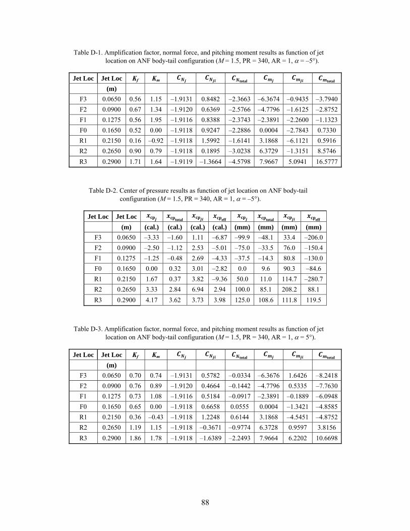
88

Table D-1. Amplification factor, normal force, and pitching moment results as function of jet location on ANF body-tail configuration (M = 1.5, PR = 340, AR = 1, = –5°).


total

(m)

F3 0.0650 0.56 1.15 –1.9131 0.8482 –2.3663 –6.3674 –0.9435 –3.7940

F2 0.0900 0.67 1.34 –1.9120 0.6369 –2.5766 –4.7796 –1.6125 –2.8752

F1 0.1275 0.56 1.95 –1.9116 0.8388 –2.3743 –2.3891 –2.2600 –1.1323

F0 0.1650 0.52 0.00 –1.9118 0.9247 –2.2886 0.0004 –2.7843 0.7330

R1 0.2150 0.16 –0.92 –1.9118 1.5992 –1.6141 3.1868 –6.1121 0.5916

R2 0.2650 0.90 0.79 –1.9118 0.1895 –3.0238 6.3729 –1.3151 8.5746

R3 0.2900 1.71 1.64 –1.9119 –1.3664 –4.5798 7.9667 5.0941 16.5777

Table D-2. Center of pressure results as function of jet location on ANF body-tail configuration (M = 1.5, PR = 340, AR = 1, = –5°).


cp cptotal cp cpeff


F3 0.0650 –3.33 –1.60 1.11 –6.87 –99.9 –48.1 33.4 –206.0

F2 0.0900 –2.50 –1.12 2.53 –5.01 –75.0 –33.5 76.0 –150.4

F1 0.1275 –1.25 –0.48 2.69 –4.33 –37.5 –14.3 80.8 –130.0

F0 0.1650 0.00 0.32 3.01 –2.82 0.0 9.6 90.3 –84.6

R1 0.2150 1.67 0.37 3.82 –9.36 50.0 11.0 114.7 –280.7

R2 0.2650 3.33 2.84 6.94 2.94 100.0 85.1 208.2 88.1

R3 0.2900 4.17 3.62 3.73 3.98 125.0 108.6 111.8 119.5

Table D-3. Amplification factor, normal force, and pitching moment results as function of jet location on ANF body-tail configuration (M = 1.5, PR = 340, AR = 1, = 5°).


total

(m)

F3 0.0650 0.70 0.74 –1.9131 0.5782 –0.0334 –6.3676 1.6426 –8.2418

F2 0.0900 0.76 0.89 –1.9120 0.4664 –0.1442 –4.7796 0.5335 –7.7630

F1 0.1275 0.73 1.08 –1.9116 0.5184 –0.0917 –2.3891 –0.1889 –6.0948

F0 0.1650 0.65 0.00 –1.9118 0.6658 0.0555 0.0004 –1.3421 –4.8585

R1 0.2150 0.36 –0.43 –1.9118 1.2248 0.6144 3.1868 –4.5451 –4.8752

R2 0.2650 1.19 1.15 –1.9118 –0.3671 –0.9774 6.3728 0.9597 3.8156

R3 0.2900 1.86 1.78 –1.9118 –1.6389 –2.2493 7.9664 6.2202 10.6698

89

Table D-4. Center of pressure results as function of jet location on ANF body-tail configuration (M = 1.5, PR = 340, AR = 1, = 5°).


cp cptotal cp cpeff


F3 0.0650 –3.33 –246.83 –2.84 –3.54 –99.9 –7404.9 –85.2 –106.2

F2 0.0900 –2.50 –53.85 –1.14 –2.94 –75.0 –1615.6 –34.3 –88.1

F1 0.1275 –1.25 –66.44 0.36 –1.85 –37.5 –1993.3 10.9 –55.5

F0 0.1650 0.00 87.60 2.02 –1.08 0.0 2627.9 60.5 –32.3

R1 0.2150 1.67 7.93 3.71 –1.98 50.0 238.0 111.3 –59.3

R2 0.2650 3.33 3.90 2.61 3.22 100.0 117.1 78.4 96.5

R3 0.2900 4.17 4.74 3.80 4.00 125.0 142.3 113.9 119.9



total

(m)

F3 0.0650 0.61 1.13 –0.6896 0.2723 –1.2602 –2.2954 –0.2924 –1.1112

F2 0.0900 0.81 1.28 –0.6885 0.1335 –1.3979 –1.7210 –0.4744 –0.7189

F1 0.1275 0.72 1.61 –0.6881 0.1922 –1.3389 –0.8600 –0.5250 0.0915

F0 0.1650 0.65 0.00 –0.6882 0.2385 –1.2926 0.0001 –0.8007 0.6759

R1 0.2150 0.52 –0.17 –0.6882 0.3272 –1.2039 1.1472 –1.3437 1.2799

R2 0.2650 1.65 1.66 –0.6883 –0.4481 –1.9792 2.2943 1.5206 5.2914

R3 0.2900 1.97 1.94 –0.6882 –0.6675 –2.1986 2.8675 2.6982 7.0423



cp cptotal cp cpeff


F3 0.0650 –3.33 –0.88 1.07 –6.20 –99.9 –26.5 32.2 –186.0

F2 0.0900 –2.50 –0.51 3.55 –3.96 –75.0 –15.4 106.6 –118.7

F1 0.1275 –1.25 0.07 2.73 –2.79 –37.5 2.0 82.0 –83.8

F0 0.1650 0.00 0.52 3.36 –1.78 0.0 15.7 100.7 –53.4

R1 0.2150 1.67 1.06 4.11 –0.54 50.0 31.9 123.2 –16.3

R2 0.2650 3.33 2.67 3.39 3.36 100.0 80.2 101.8 100.7

R3 0.2900 4.17 3.20 4.04 4.11 125.0 96.1 121.3 123.2

90



total

(m)

F3 0.0650 0.67 0.98 –0.6891 0.2292 0.3830 –2.2937 0.0497 –3.7205

F2 0.0900 0.74 1.16 –0.6883 0.1774 0.3320 –1.7206 –0.2765 –3.4736

F1 0.1275 0.70 1.47 –0.6881 0.2034 0.3583 –0.8599 –0.4048 –2.7412

F0 0.1650 0.76 0.00 –0.6881 0.1662 0.3210 0.0002 –0.4626 –1.9389

R1 0.2150 0.65 0.11 –0.6882 0.2383 0.3930 1.1471 –1.0244 –1.3538

R2 0.2650 1.68 1.73 –0.6882 –0.4684 –0.3137 2.2940 1.6733 2.4908

R3 0.2900 1.75 1.71 –0.6882 –0.5152 –0.3605 2.8675 2.0383 3.4293



cp cptotal cp cpeff


F3 0.0650 –3.33 9.71 –0.22 –4.88 –99.9 291.4 –6.5 –146.4

F2 0.0900 –2.50 10.46 1.56 –3.91 –75.0 313.9 46.8 –117.3

F1 0.1275 –1.25 7.65 1.99 –2.61 –37.5 229.5 59.7 –78.3

F0 0.1650 0.00 6.04 2.78 –0.89 0.0 181.2 83.5 –26.6

R1 0.2150 1.67 3.44 4.30 0.27 50.0 103.3 129.0 8.2

R2 0.2650 3.33 7.94 3.57 3.43 100.0 238.2 107.2 102.9

R3 0.2900 4.17 9.51 3.96 4.08 125.0 285.4 118.7 122.3



total

(m)

F3 0.0650 0.59 1.20 –0.3520 0.1455 –0.9257 –1.1716 –0.2300 –0.5179

F2 0.0900 0.82 1.38 –0.3513 0.0648 –1.0057 –0.8781 –0.3359 –0.3303

F1 0.1275 0.75 1.80 –0.3511 0.0868 –0.9836 –0.4388 –0.3527 0.0921

F0 0.1650 0.76 0.00 –0.3511 0.0853 –0.9851 0.0001 –0.3773 0.5065

R1 0.2150 0.73 0.23 –0.3512 0.0933 –0.9771 0.5854 –0.4494 1.0197

R2 0.2650 2.18 2.31 –0.3512 –0.4129 –1.4833 1.1707 1.5354 3.5898

R3 0.2900 1.69 1.67 –0.3511 –0.2408 –1.3112 1.4632 0.9759 3.3227

91



cp cptotal cp cpeff


F3 0.0650 –3.33 –0.56 1.58 –6.79 –99.9 –16.8 47.4 –203.7

F2 0.0900 –2.50 –0.33 5.18 –4.24 –75.0 –9.9 155.5 –127.1

F1 0.1275 –1.25 0.09 4.06 –2.99 –37.5 2.8 121.9 –89.8

F0 0.1650 0.00 0.51 4.42 –1.42 0.0 15.4 132.7 –42.6

R1 0.2150 1.67 1.04 4.82 0.53 50.0 31.3 144.5 15.8

R2 0.2650 3.33 2.42 3.72 3.54 100.0 72.6 111.6 106.2

R3 0.2900 4.17 2.53 4.05 4.12 125.0 76.0 121.6 123.6



total

(m)

F3 0.0650 0.81 1.16 –0.3515 0.0654 0.4331 –1.1701 –0.1855 –2.2393

F2 0.0900 0.94 1.23 –0.3512 0.0224 0.3905 –0.8779 –0.2010 –1.9626

F1 0.1275 0.93 1.40 –0.3511 0.0240 0.3922 –0.4388 –0.1738 –1.4963

F0 0.1650 0.97 0.00 –0.3511 0.0098 0.3779 0.0001 –0.1303 –1.0139

R1 0.2150 0.99 0.80 –0.3511 0.0023 0.3704 0.5853 –0.1187 –0.4170

R2 0.2650 1.78 1.88 –0.3512 –0.2732 0.0949 1.1706 1.0247 1.3116

R3 0.2900 1.72 1.67 –0.3511 –0.2513 0.1169 1.4631 0.9827 1.5621



cp cptotal cp cpeff


F3 0.0650 –3.33 5.17 2.84 –4.74 –99.9 155.1 85.1 –142.1

F2 0.0900 –2.50 5.03 8.97 –3.28 –75.0 150.8 269.1 –98.5

F1 0.1275 –1.25 3.81 7.23 –1.87 –37.5 114.4 216.8 –56.2

F0 0.1650 0.00 2.68 13.30 –0.38 0.0 80.5 399.0 –11.4

R1 0.2150 1.67 1.13 50.72 1.34 50.0 33.8 1521.6 40.1

R2 0.2650 3.33 –13.82 3.75 3.52 100.0 –414.5 112.5 105.5

R3 0.2900 4.17 –13.36 3.91 4.06 125.0 –400.9 117.3 121.8

92


93

Appendix E. Army-Navy Finner Tabulated Results at = ±2.5°

94

Table E-1. Amplification factor, normal force, and pitching moment results as function of jet location on ANF body-tail configuration (M = 2.5, PR = 340, AR = 1, = –2.5°).


total

(m)

F3 0.0650 0.62 1.07 –0.6895 0.2647 –0.8304 –2.2949 –0.1578 –1.7357

F2 0.0900

F1 0.1275 0.74 1.49 –0.6881 0.1765 –0.9173 –0.8600 –0.4237 –0.5666

F0 0.1650 0.68 0.00 –0.6882 0.2225 –0.8713 0.0001 –0.7073 0.0099

R1 0.2150

R2 0.2650

R3 0.2900 1.79 1.81 –0.6882 –0.5426 –1.6364 2.8675 2.3359 5.9206

Table E-2. Center of pressure results as function of jet location on ANF body-tail configuration (M = 2.5, PR = 340, AR = 1, = –2.5°).


cp cptotal cp cpeff


F3 0.0650 –3.33 –2.09 0.60 –5.77 –99.9 –62.7 17.9 –173.2

F2 0.0900 –2.50

F1 0.1275 –1.25 –0.62 2.40 –2.51 –37.5 –18.5 72.0 –75.3

F0 0.1650 0.00 0.01 3.18 –1.52 0.0 0.3 95.4 –45.6

R1 0.2150 1.67

R2 0.2650 3.33

R3 0.2900 4.17 3.62 4.31 4.23 125.0 108.5 129.2 126.8

95

Table E-3. Amplification factor, normal force, and pitching moment results as function of jet location on ANF body-tail configuration (M = 2.5, PR = 340, AR = 1, = 2.5°).


total

(m)

F3 0.0650 0.70 0.97 –0.6892 0.2073 –0.0763 –2.2941 0.0605 –2.9507

F2 0.0900

F1 0.1275 0.69 1.51 –0.6881 0.2103 –0.0722 –0.8600 –0.4395 –2.0165

F0 0.1650 0.72 0.00 –0.6881 0.1905 –0.0919 0.0002 –0.5572 –1.2742

R1 0.2150

R2 0.2650

R3 0.2900 1.75 1.72 –0.6882 –0.5165 –0.7990 2.8674 2.0614 4.2118

Table E-4. Center of pressure results as function of jet location on ANF body-tail configuration (M = 2.5, PR = 340, AR = 1, = 2.5°).


cp cptotal cp cpeff


F3 0.0650 –3.33 –38.69 –0.29 –4.64 –99.9 –1160.8 –8.7 –139.1

F2 0.0900 –2.50

F1 0.1275 –1.25 –27.94 2.09 –2.72 –37.5 –838.3 62.7 –81.6

F0 0.1650 0.00 –13.86 2.92 –1.12 0.0 –415.7 87.7 –33.6

R1 0.2150 1.67

R2 0.2650 3.33

R3 0.2900 4.17 5.27 3.99 4.09 125.0 158.1 119.7 122.7

96


97

List of Symbols, Abbreviations, and Acronyms

3-D three-dimensional

6DOF six degree-of-freedom

Ae jet nozzle exit area, m2

At jet nozzle throat area, m2

ANF Army-Navy Finner

AR jet exit area to throat area ratio, /

ARL U.S. Army Research Laboratory

cal. caliber

CFD computational fluid dynamics

CFL Courant-Freidrichs-Lewy

c.g. or CG projectile center of gravity, m or caliber

CKE cubic k-e nonlinear turbulence model

jet thrust force coefficient

jet interaction force coefficient

total total normal force coefficient (thrust + interaction)

pitching moment coefficient due to jet interaction force

pitching moment coefficient due to jet thrust force

total total pitching moment coefficient (thrust + interaction)

CONTRAJ control trajectory model

CPU central processing unit

CVP counter-rotating vortex pair

projectile diameter, m

98

DOD Department of Defense

DSRC DOD Supercomputing Resource Center

jet interaction force, N

jet thrust force, N

total total normal force (thrust + interaction), N

no-jet normal force without jet, N

GN&C guidance navigation and control

HLLC Harten-Lax-Van Leer-Contact

J jet exit to freestream dynamic pressure ratio

JI jet interaction

KER Goldberg’s k--Rt turbulence model

jet force amplification factor

jet moment amplification factor

M Mach number

moment induced by jet interaction force, N-m

moment induced by jet thrust force, N-m

total moment induced by total normal force, N-m

MIME Multipurpose Intelligent Meshing Environment

local static pressure, Pa

freestream static pressure, Pa

freestream total pressure, Pa

jet total pressure, Pa

PIV particle image velocimetry

PR jet total to freestream static pressure ratio, /

99

PR0 jet total to freestream total pressure ratio, /

PRODAS projectile, design, and analysis software

QE quadrant elevation, °

RANS Reynolds-Averaged Navier-Stokes

RJC reaction jet control

RKE realizable k- turbulence model

RSM Reynolds Stress Transport turbulence model

RT Goldberg’s Rt turbulence model

s second

SA Spalart-Allmaras turbulence model

SBLI shock-boundary layer interaction

SL sea level

SST Menter’s Shear Stress Transport turbulence model

STP standard temperature and pressure

freestream static temperature, K

freestream total temperature, K

jet total temperature, K

TVD Total-Variation-Diminishing

x distance along symmetry plane flate plate, mm

cp center of pressure due to total, jet, interaction forces, etc., cal.

y+ dimensionless wall distance

z lateral distance away from flate plate jet orifice, mm

angle of attack, °

total angle of attack, , °

100

eddy diffusivity, m2-s-1

azimuthal distance around projectile body, °

specific dissipation (turbulence), or vorticity, s-1

NO. OF NO. OF COPIES ORGANIZATION COPIES ORGANIZATION

101

1 DEFENSE TECHNICAL (PDF) INFORMATION CTR DTIC OCA 1 DIRECTOR (PDF) US ARMY RESEARCH LAB IMAL HRA 1 DIRECTOR (PDF) US ARMY RESEARCH LAB RDRL CIO LL 1 GOVT PRINTG OFC (PDF) A MALHOTRA 6 RDECOM AMRDEC (PDF) L AUMAN J DOYLE S DUNBAR B GRANTHAM M MCDANIEL C ROSEMA 16 RDECOM ARDEC (PDF) D CARLUCCI S CHUNG D CLER M DUCA L FLORIO J GRAU M HOLLIS W KOENIG A LICHTENBERG-SCANLAN G MALEJKO T RECCHIA C STOUT W TOLEDO J TRAVAILLE E VAZQUEZ C WILSON 4 PM CAS (PDF) M BURKE R KIEBLER P MANZ G SCHWARTZ

3 PM MAS (PDF) J FOULTZ C GRASSANO D RIGOGLIOSO

1 AEROPREDICTION INC (PDF) F MOORE 1 ARROW TECH (PDF) W HATHAWAY 1 NASA LANGLEY RSRCH CTR (PDF) S VIKEN 3 NAVAIR (PDF) D FINDLAY J LEE T SHAFER 2 NAWCWD (PDF) P CROSS R SCHULTZ 1 AFOSR EOARD (PDF) G ABATE 2 NSWC DAHLGREN (PDF) L STEELMAN K PAMADI 41 DIR USARL (PDF) RDRL WM P BAKER R EHLERS P PLOSTINS RDRL WML P PEREGINO M ZOLTOSKI RDRL WML A W OBERLE L STROHM RDRL WML B N TRIVEDI RDRL WML C S AUBERT RDRL WML D R BEYER M NUSCA RDRL WML E V BHAGWANDIN I CELMINS J DESPIRITO L FAIRFAX F FRESCONI J GARNER B GUIDOS K HEAVEY R KEPPINGER G OBERLIN

NO. OF COPIES ORGANIZATION

102

T PUCKETT J SAHU S SILTON P WEINACHT RDRL WML F G BROWN J CONDON B DAVIS PL HUFNAL B KLINE J MALEY B NELSON B TOPPER RDRL WML G M CHEN C EICHHORST M MINNICINO J SOUTH RDRLWML H J NEWILL RDRL WMM J ZABINSKI RDRL WMP D LYON RDRL WMP G R BANTON 2 DEFENCE SCI AND TECHLGY LAB (PDF) (DSTL) R CHAPLIN B SHOESMITH 3 DEFENCE SCI AND TECHLGY (PDF) ORGANIZATION (DSTO) S HENBEST M GIACOBELLO B WOODYATT 1 DEFENCE TECHLGY AGENCY (DTA) (PDF) N WILLIAMS 2 INSTITUTE SAINT LOUIS (ISL) (PDF) C BERNER P GNEMMI 2 DEFENCE RSRCH AND DEV (PDF) CANADA (DRDC) D CORRIVEAU N HAMEL

lateral reaction jet flow interaction effects on a generic … reaction jet flow interaction effects...

Documents