Latent class analysis with Stata

Isabel CanettePrincipal Mathematician and Statistician

StataCorp LLC

2018 Mexican Stata Users Group MeetingTlaxcala, August 16-17, 2018

Introduction

“Latent class analysis” (LCA) comprises a set of techniques used tomodel situations where there are different subgroups of individuals,and group memebership is not directly observed, for example:.

I Social sciences: a population where different subgroups havedifferent motivations to drink.

I Medical sciences: using available data to identify subgroups ofrisk for diabetes.

I Survival analysis: subgroups that are vulnerable to differenttypes of risks (competing risks).

I Education: identifying groups of students with differentlearning skills.

I Market research: identifying different kinds of consumers.

The scope of the term “latent class analysis” varies widely fromsource to source.

Collin and Lanza (2010) discuss some of the models that areusually considered LCA. Also, they point out: “ In this book, whenwe refer to latent class models we mean models in which the latentvariable is categorical and the indicators are treated as categorical”.

In Stata, we use “ LCA” to refer to a wide array of models wherethere are two or more unobserved classes

I Dependent variables might follow any of the distributionssupported by gsem, as logistic, Gaussian, Poisson,multinomial, negative binomial, Weibull, etc.(help gsemfamily and link options)

I There might be covariates (categorical or continuos) to explainthe dependent variables

I There might be covariates to explain class membership

Stata adopts a model-based approach to LCA. In this context, wecan see LCA as group analysis where the groups are unknown.

Let’s see an example, first with groups and then with classes:

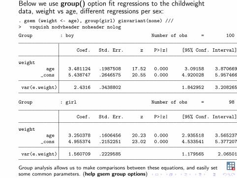
Below we use group() option fit regressions to the childweightdata, weight vs age, different regressions per sex:. gsem (weight <- age), group(girl) ginvariant(none) ///> vsquish nodvheader noheader nolog

Group : boy Number of obs = 100

Coef. Std. Err. z P>|z| [95% Conf. Interval]

weightage 3.481124 .1987508 17.52 0.000 3.09158 3.870669

_cons 5.438747 .2646575 20.55 0.000 4.920028 5.957466

var(e.weight) 2.4316 .3438802 1.842952 3.208265

Group : girl Number of obs = 98

Coef. Std. Err. z P>|z| [95% Conf. Interval]

weightage 3.250378 .1606456 20.23 0.000 2.935518 3.565237

_cons 4.955374 .2152251 23.02 0.000 4.533541 5.377207

var(e.weight) 1.560709 .2229585 1.179565 2.06501

Group analysis allows us to make comparisons between these equations, and easily setsome common parameters. (help gsem group options)

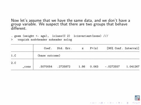
Now let’s assume that we have the same data, and we don’t have agroup variable. We suspect that there are two groups that behavedifferent.

. gsem (weight <- age), lclass(C 2) lcinvariant(none) ///> vsquish nodvheader noheader nolog

Coef. Std. Err. z P>|z| [95% Conf. Interval]

1.C (base outcome)

2.C_cons .5070054 .2725872 1.86 0.063 -.0272557 1.041267

Class : 1

Coef. Std. Err. z P>|z| [95% Conf. Interval]

weightage 5.938576 .2172374 27.34 0.000 5.512798 6.364353

_cons 3.8304 .2198091 17.43 0.000 3.399582 4.261218

var(e.weight) .6766618 .1817454 .3997112 1.145505

Class : 2

Coef. Std. Err. z P>|z| [95% Conf. Interval]

weightage 2.90492 .2375441 12.23 0.000 2.439342 3.370498

_cons 5.551337 .4567506 12.15 0.000 4.656122 6.446551

var(e.weight) 1.52708 .2679605 1.082678 2.153893

The second table on the LCA model same structure as the outputfrom the group model.

In addition, the LCA output starts with a table corresponding tothe class estimation. This is a binary (logit) model used to find thetwo classes.

In the latent class model all the equations are estimated jointly andall parameters affect each other, even when we estimate differentparameters per class.

How do we interpret these classes? We need to analyze our classesand see how they relate to other variables in the data. Also, wemight interpret our classes in terms of a previous theory, providedthat our analysis is in agreement with the theory. We will seepost-estimation commands that implement the usual tools used forthis task.

Let’s compute the class predictions based on the posteriorprobability.

. predict postp*, classposteriorpr

. generate pclass = 1 + (postp2>0.5)

. tabulate pclass

pclass Freq. Percent Cum.

1 78 39.39 39.392 120 60.61 100.00

Total 198 100.00

. tabulate pclass girl

genderpclass boy girl Total

1 40 38 782 60 60 120

Total 100 98 198

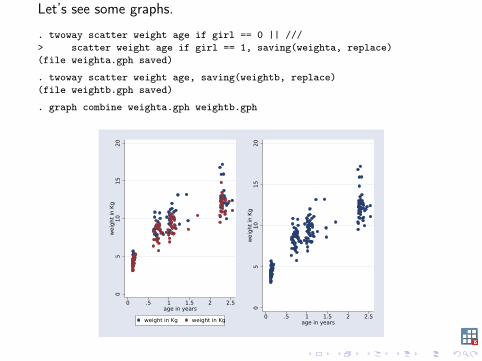
Let’s see some graphs.

. twoway scatter weight age if girl == 0 || ///> scatter weight age if girl == 1, saving(weighta, replace)(file weighta.gph saved)

. twoway scatter weight age, saving(weightb, replace)(file weightb.gph saved)

. graph combine weighta.gph weightb.gph0

510

1520

wei

ght i

n Kg

0 .5 1 1.5 2 2.5age in years

weight in Kg weight in Kg

05

1015

20w

eigh

t in

Kg

0 .5 1 1.5 2 2.5age in years

. predict mu*, mu

. twoway scatter weight age if pclass ==1 || ///> scatter weight age if pclass ==2 || ///> line mu1 age if pclass ==1 || ///> line mu2 age if pclass ==2 , legend(off)

05

1015

20

0 .5 1 1.5 2 2.5age in years

gsem did exactly what we asked for: tell me what are the two morelikely groups for two different linear regressions.

This approach allows us to generalize LCA in different directions,for example, if we had more information:

I we could incorporate more than one equation:. gsem (weight <- age ) (height <- age ), ///> lclass(C 3) lcinvariant(none)

I we could incorporate class predictors:. gsem (weight <- age ) (height <- age ), ///(C <- diet_quality) lclass(C 2) lcinvariant(none)

EstimationFor a dependent variables y = y1, . . . yn and g groups for a givenobservation (i.e. no observation index below), the likelihood iscomputed as:

f (y) =

g∑i=1

πi fi (y|zi ),where :

I zi is the vector of linear forms for class i , i.e., ziji = x′βij ,where x are the dependent variables, and βij are thecoefficients for main equation j , (conditional on) class i .

I fi is the joint likelihood of y = y1, . . . yn conditional on class iI the probabilities of belonging to each class πi , i = 1, . . . , g are

computed using a multinomial model,

πi =exp(γi )∑g

k=1 exp(γk).

γk , k = 2, . . . g is the linear form class k in the latentclass equation, γ1 = 1.

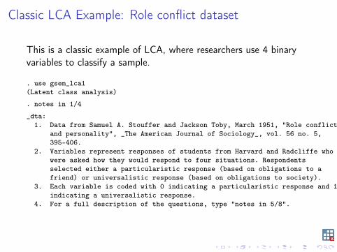
Classic LCA Example: Role conflict dataset

This is a classic example of LCA, where researchers use 4 binaryvariables to classify a sample.

. use gsem_lca1(Latent class analysis)

. notes in 1/4

_dta:1. Data from Samuel A. Stouffer and Jackson Toby, March 1951, "Role conflict

and personality", _The American Journal of Sociology_, vol. 56 no. 5,395-406.

2. Variables represent responses of students from Harvard and Radcliffe whowere asked how they would respond to four situations. Respondentsselected either a particularistic response (based on obligations to afriend) or universalistic response (based on obligations to society).

3. Each variable is coded with 0 indicating a particularistic response and 1indicating a universalistic response.

4. For a full description of the questions, type "notes in 5/8".

. describe

Contains data from gsem_lca1.dtaobs: 216 Latent class analysis

vars: 4 10 Oct 2017 12:46size: 864 (_dta has notes)

storage display valuevariable name type format label variable label

accident byte %9.0g would testify against friend inaccident case

play byte %9.0g would give negative review offriend´s play

insurance byte %9.0g would disclose health concerns tofriend´s insurance company

stock byte %9.0g would keep company secret fromfriend

Sorted by: accident play insurance stock

. list in 120/121

accident play insura~e stock

120. 1 0 1 1121. 1 1 0 0

For each observation, we have a vector of responsesY = (Y1,Y2,Y2,Y4) (I am omitting an observation index)The traditional approach deals with models that involve onlycategorical variables, so within each class we have 2n cells withzeros and ones, and probabilities are estimates nonparametrically.

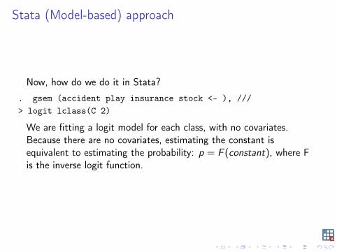
Stata (Model-based) approach

Now, how do we do it in Stata?

. gsem (accident play insurance stock <- ), ///> logit lclass(C 2)

We are fitting a logit model for each class, with no covariates.Because there are no covariates, estimating the constant isequivalent to estimating the probability: p = F (constant), where Fis the inverse logit function.

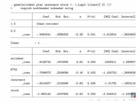
. gsem(accident play insurance stock <- ),logit lclass(C 2) ///> vsquish nodvheader noheader nolog

Coef. Std. Err. z P>|z| [95% Conf. Interval]

1.C (base outcome)

2.C_cons -.9482041 .2886333 -3.29 0.001 -1.513915 -.3824933

Class : 1

Coef. Std. Err. z P>|z| [95% Conf. Interval]

accident_cons .9128742 .1974695 4.62 0.000 .5258411 1.299907

play_cons -.7099072 .2249096 -3.16 0.002 -1.150722 -.2690926

insurance_cons -.6014307 .2123096 -2.83 0.005 -1.01755 -.1853115

stock_cons -1.880142 .3337665 -5.63 0.000 -2.534312 -1.225972

Coef. Std. Err. z P>|z| [95% Conf. Interval]

Class : 2

Coef. Std. Err. z P>|z| [95% Conf. Interval]

accident_cons 4.983017 3.745987 1.33 0.183 -2.358982 12.32502

play_cons 2.747366 1.165853 2.36 0.018 .4623372 5.032395

insurance_cons 2.534582 .9644841 2.63 0.009 .6442279 4.424936

stock_cons 1.203416 .5361735 2.24 0.025 .1525356 2.254297

From the output, parameters for the second class are larger thanthose on the first class. Postestimation commands will help us tointerpret this output.

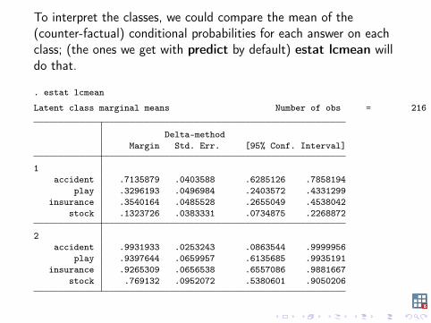
To interpret the classes, we could compare the mean of the(counter-factual) conditional probabilities for each answer on eachclass; (the ones we get with predict by default) estat lcmean willdo that.

. estat lcmean

Latent class marginal means Number of obs = 216

Delta-methodMargin Std. Err. [95% Conf. Interval]

1accident .7135879 .0403588 .6285126 .7858194

play .3296193 .0496984 .2403572 .4331299insurance .3540164 .0485528 .2655049 .4538042

stock .1323726 .0383331 .0734875 .2268872

2accident .9931933 .0253243 .0863544 .9999956

play .9397644 .0659957 .6135685 .9935191insurance .9265309 .0656538 .6557086 .9881667

stock .769132 .0952072 .5380601 .9050206

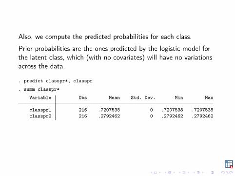
Also, we compute the predicted probabilities for each class.

Prior probabilities are the ones predicted by the logistic model forthe latent class, which (with no covariates) will have no variationsacross the data.

. predict classpr*, classpr

. summ classpr*

Variable Obs Mean Std. Dev. Min Max

classpr1 216 .7207538 0 .7207538 .7207538classpr2 216 .2792462 0 .2792462 .2792462

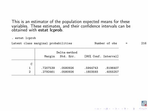
This is an estimator of the population expected means for thesevariables. These estimates, and their confidence intervals can beobtained with estat lcprob.

. estat lcprob

Latent class marginal probabilities Number of obs = 216

Delta-methodMargin Std. Err. [95% Conf. Interval]

C1 .7207539 .0580926 .5944743 .81964072 .2792461 .0580926 .1803593 .4055257

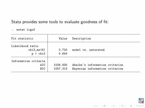
Stata provides some tools to evaluate goodness of fit:

. estat lcgof

Fit statistic Value Description

Likelihood ratiochi2_ms(6) 2.720 model vs. saturated

p > chi2 0.843

Information criteriaAIC 1026.935 Akaike´s information criterionBIC 1057.313 Bayesian information criterion

Concluding remarks:I gsem offers a framework where we can fit models accounting

for latent classes.I Responses might take one or more of the distributions

supported by gsem.I Discrete latent variables might have more than two groups,

and more than one latent variable also might be included.I Latent class models that have one dependent variable, can be

seen as finite mixture models. The fmm prefix allows us toeasily fit finite mixture models for a variety of distributions.

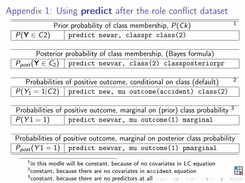
Appendix 1: Using predict after the role conflict datasetPrior probability of class membership, P(Ck) 1

P(Y ∈ C2) predict newar, classpr class(2)

Posterior probability of class membership, (Bayes formula)Ppost(Y ∈ C2) predict newvar, class(2) classposteriorpr

Probabilities of positive outcome, conditional on class (default) 2

P(Y1 = 1|C2) predict new, mu outcome(accident) class(2)

Probabilities of positive outcome, marginal on (prior) class probability 3

P(Y 1 = 1) predict newvar, mu outcome(1) marginal

Probabilities of positive outcome, marginal on posterior class probabilityPpost(Y 1 = 1) predict newvar, mu outcome(1) pmarginal

1in this modle will be constant, because of no covariates in LC equation2constant, because there are no covariates in accident equation3constant, because there are no predictors at all

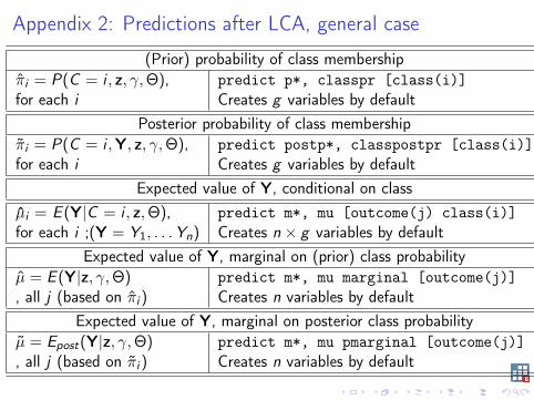
Appendix 2: Predictions after LCA, general case

(Prior) probability of class membershipπ̂i = P(C = i , z, γ,Θ), predict p*, classpr [class(i)]for each i Creates g variables by default

Posterior probability of class membershipπ̃i = P(C = i ,Y, z, γ,Θ), predict postp*, classpostpr [class(i)]for each i Creates g variables by default

Expected value of Y, conditional on classµ̂i = E (Y|C = i , z,Θ), predict m*, mu [outcome(j) class(i)]for each i ;(Y = Y1, . . .Yn) Creates n × g variables by default

Expected value of Y, marginal on (prior) class probabilityµ̂ = E (Y|z, γ,Θ) predict m*, mu marginal [outcome(j)], all j (based on π̂i ) Creates n variables by default

Expected value of Y, marginal on posterior class probabilityµ̃ = Epost(Y|z, γ,Θ) predict m*, mu pmarginal [outcome(j)], all j (based on π̃i ) Creates n variables by default