latent class analysis for intensive longitudinal data ... · hidden markov processes, regime...
TRANSCRIPT
Latent class analysis for intensive longitudinal data,Hidden Markov processes, Regime switching
models and Dynamic Structural Equations in Mplus
Tihomir Asparouhov, Bengt Muthen and Ellen Hamaker
May 24, 2016
Tihomir Asparouhov, Bengt Muthen and Ellen Hamaker Muthen & Muthen 1/ 61
Overview
Motivation
Dynamic Structural Equations Model (DSEM) framework andestimation
New Multilevel Mixture Models: these are needed as buildingblock for the more advanced models
Single level models: HMM (Hidden Markov Models), MSAR(Markov Switching Auto-Regressive), MSKF (MarkovSwitching Kalman Filter)
Two-level HMM, MSAR, MSKF
Tihomir Asparouhov, Bengt Muthen and Ellen Hamaker Muthen & Muthen 2/ 61
Motivation
Merge ”time series”, ”structural equation”, ”multilevel” and”mixture” modeling concepts in a generalized modelingframework in Mplus V8
In this context two-level means single-level. Cluster is alwaysthe individual. Many observations are collected within subjectand analyzed in long format. Most time-series models weredeveloped for single level data however most social scienceapplications need two-level methods because we study manyindividuals across time, rather than the US economy across time.
Mplus release timeline: V8 will have DSEM and probably singlelevel MSAR. V8.1 will have two-level MSAR.
Tihomir Asparouhov, Bengt Muthen and Ellen Hamaker Muthen & Muthen 3/ 61
Motivation continued
Consider the following hypothetical example. A group ofdepression patients answer daily a brief survey to evaluate theircurrent state. Based on current observations, past history, mostrecent history, similar behavior from other patients we classifythe patient in one of 3 states:
S1: OKS2: Stretch of poor outcomes, needs doctor visit/evaluationS3: At risk for suicide, needs hospitalization
Future of health care? Cheaper, smarter and more effective?
The models we describe in this talk can be used to model thedata from this hypothetical example: combine mixture,multilevel, time-series, latent variables, and structural models.
Tihomir Asparouhov, Bengt Muthen and Ellen Hamaker Muthen & Muthen 4/ 61
Motivation continued
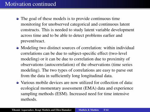
The goal of these models is to provide continuous timemonitoring for unobserved categorical and continuous latentconstructs. This is needed to study latent variable developmentacross time and to be able to detect problems earlier andprevent/react.
Modeling two distinct sources of correlation: within individualcorrelations can be due to subject-specific effect (two-levelmodeling) or it can be due to correlation due to proximity ofobservations (autocorrelation) of the observations (time seriesmodeling). The two types of correlations are easy to parse outfrom the data in sufficiently long longitudinal data.
Various mobile devices are now utilized for collection of data:ecological momentary assessment (EMA) data and experiencesampling methods (ESM). Increased need for time intensivemethods.
Tihomir Asparouhov, Bengt Muthen and Ellen Hamaker Muthen & Muthen 5/ 61
Mplus general DSEM framework
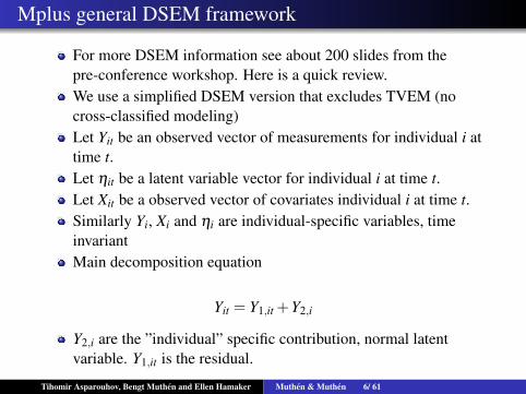
For more DSEM information see about 200 slides from thepre-conference workshop. Here is a quick review.We use a simplified DSEM version that excludes TVEM (nocross-classified modeling)Let Yit be an observed vector of measurements for individual i attime t.Let ηit be a latent variable vector for individual i at time t.Let Xit be a observed vector of covariates individual i at time t.Similarly Yi, Xi and ηi are individual-specific variables, timeinvariantMain decomposition equation
Yit = Y1,it +Y2,i
Y2,i are the ”individual” specific contribution, normal latentvariable. Y1,it is the residual.
Tihomir Asparouhov, Bengt Muthen and Ellen Hamaker Muthen & Muthen 6/ 61
DSEM framework continued
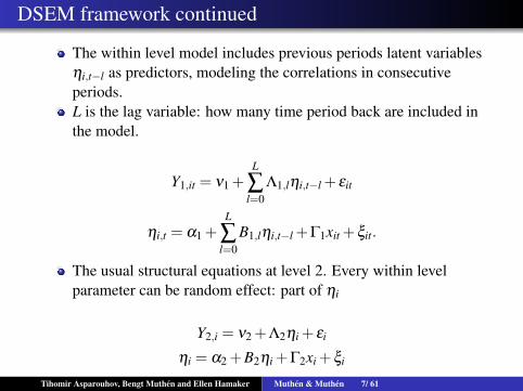
The within level model includes previous periods latent variablesηi,t−l as predictors, modeling the correlations in consecutiveperiods.L is the lag variable: how many time period back are included inthe model.
Y1,it = ν1 +L
∑l=0
Λ1,lηi,t−l + εit
ηi,t = α1 +L
∑l=0
B1,lηi,t−l +Γ1xit +ξit.
The usual structural equations at level 2. Every within levelparameter can be random effect: part of ηi
Y2,i = ν2 +Λ2ηi + εi
ηi = α2 +B2ηi +Γ2xi +ξi
Tihomir Asparouhov, Bengt Muthen and Ellen Hamaker Muthen & Muthen 7/ 61

DSEM framework continued
Observed variables can also have lag variables and can be usedas predictors.
Ordered polytomous and binary dependent variables are includedin this framework using the underlying Y∗ approach: probit link
The model is also of interest when N=1. No second level. Allobservations are correlated. Multivariate econometrics models.
The N = 1 model can be used also on the data from a singleindividual to construct a psychological profile and match it to theknown profile of a psychological disorder.
We use Bayes estimation
The above model has variables with negative or zero indices. Wetreat those as auxiliary parameters that have prior distribution.Automatic option specification is implemented in Mplus.
Tihomir Asparouhov, Bengt Muthen and Ellen Hamaker Muthen & Muthen 8/ 61
DSEM Mixture Model
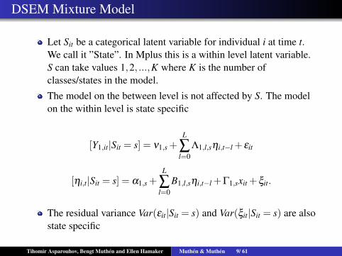
Let Sit be a categorical latent variable for individual i at time t.We call it ”State”. In Mplus this is a within level latent variable.S can take values 1,2, ...,K where K is the number ofclasses/states in the model.
The model on the between level is not affected by S. The modelon the within level is state specific
[Y1,it|Sit = s] = ν1,s +L
∑l=0
Λ1,l,sηi,t−l + εit
[ηi,t|Sit = s] = α1,s +L
∑l=0
B1,l,sηi,t−l +Γ1,sxit +ξit.
The residual variance Var(εit|Sit = s) and Var(ξit|Sit = s) are alsostate specific
Tihomir Asparouhov, Bengt Muthen and Ellen Hamaker Muthen & Muthen 9/ 61
DSEM Mixture Model Continued
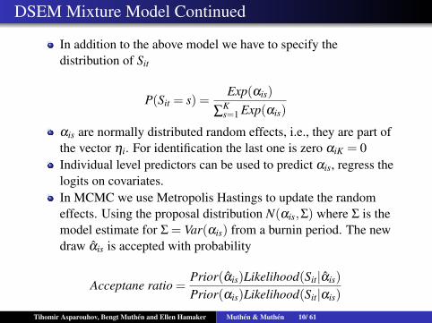
In addition to the above model we have to specify thedistribution of Sit
P(Sit = s) =Exp(αis)
∑Ks=1 Exp(αis)
αis are normally distributed random effects, i.e., they are part ofthe vector ηi. For identification the last one is zero αiK = 0Individual level predictors can be used to predict αis, regress thelogits on covariates.In MCMC we use Metropolis Hastings to update the randomeffects. Using the proposal distribution N(αis,Σ) where Σ is themodel estimate for Σ = Var(αis) from a burnin period. The newdraw αis is accepted with probability
Acceptane ratio =Prior(αis)Likelihood(Sit|αis)
Prior(αis)Likelihood(Sit|αis)
Tihomir Asparouhov, Bengt Muthen and Ellen Hamaker Muthen & Muthen 10/ 61
DSEM Mixture Model Continued
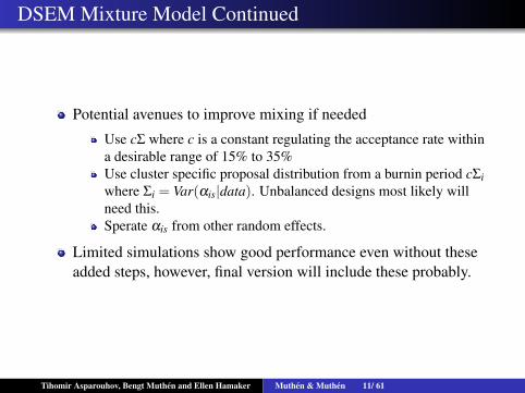
Potential avenues to improve mixing if needed
Use cΣ where c is a constant regulating the acceptance rate withina desirable range of 15% to 35%Use cluster specific proposal distribution from a burnin period cΣiwhere Σi = Var(αis|data). Unbalanced designs most likely willneed this.Sperate αis from other random effects.
Limited simulations show good performance even without theseadded steps, however, final version will include these probably.
Tihomir Asparouhov, Bengt Muthen and Ellen Hamaker Muthen & Muthen 11/ 61
Bayes Multilevel Mixture Model
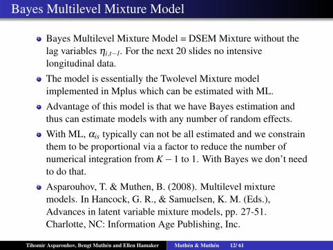
Bayes Multilevel Mixture Model = DSEM Mixture without thelag variables ηi,t−l. For the next 20 slides no intensivelongitudinal data.
The model is essentially the Twolevel Mixture modelimplemented in Mplus which can be estimated with ML.
Advantage of this model is that we have Bayes estimation andthus can estimate models with any number of random effects.
With ML, αis typically can not be all estimated and we constrainthem to be proportional via a factor to reduce the number ofnumerical integration from K−1 to 1. With Bayes we don’t needto do that.
Asparouhov, T. & Muthen, B. (2008). Multilevel mixturemodels. In Hancock, G. R., & Samuelsen, K. M. (Eds.),Advances in latent variable mixture models, pp. 27-51.Charlotte, NC: Information Age Publishing, Inc.
Tihomir Asparouhov, Bengt Muthen and Ellen Hamaker Muthen & Muthen 12/ 61
LCA with clustered data
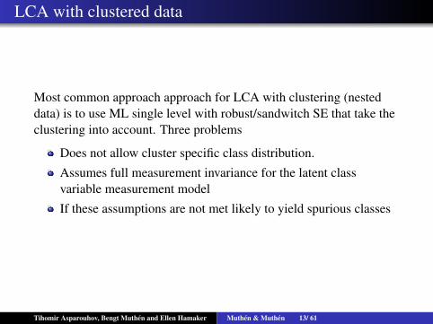
Most common approach approach for LCA with clustering (nesteddata) is to use ML single level with robust/sandwitch SE that take theclustering into account. Three problems
Does not allow cluster specific class distribution.
Assumes full measurement invariance for the latent classvariable measurement model
If these assumptions are not met likely to yield spurious classes
Tihomir Asparouhov, Bengt Muthen and Ellen Hamaker Muthen & Muthen 13/ 61
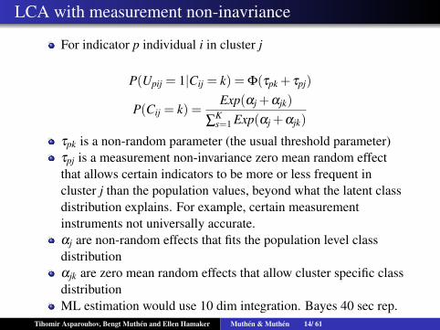
LCA with measurement non-inavriance
For indicator p individual i in cluster j
P(Upij = 1|Cij = k) = Φ(τpk + τpj)
P(Cij = k) =Exp(αj +αjk)
∑Ks=1 Exp(αj +αjk)
τpk is a non-random parameter (the usual threshold parameter)τpj is a measurement non-invariance zero mean random effectthat allows certain indicators to be more or less frequent incluster j than the population values, beyond what the latent classdistribution explains. For example, certain measurementinstruments not universally accurate.αj are non-random effects that fits the population level classdistributionαjk are zero mean random effects that allow cluster specific classdistributionML estimation would use 10 dim integration. Bayes 40 sec rep.
Tihomir Asparouhov, Bengt Muthen and Ellen Hamaker Muthen & Muthen 14/ 61
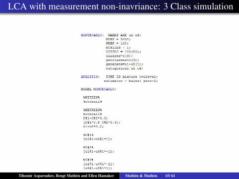
LCA with measurement non-inavriance: 3 Class simulation
Tihomir Asparouhov, Bengt Muthen and Ellen Hamaker Muthen & Muthen 15/ 61
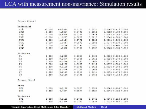
LCA with measurement non-inavriance: Simulation results
Tihomir Asparouhov, Bengt Muthen and Ellen Hamaker Muthen & Muthen 16/ 61
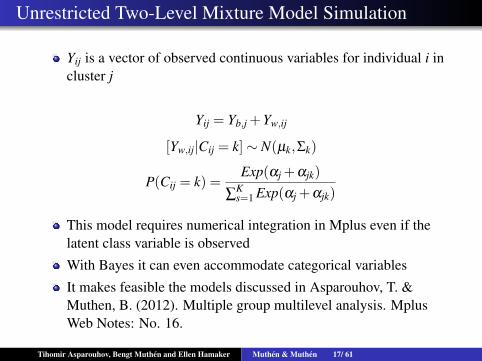
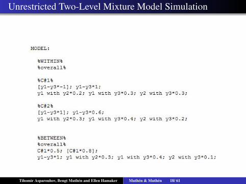
Unrestricted Two-Level Mixture Model Simulation
Yij is a vector of observed continuous variables for individual i incluster j
Yij = Yb,j +Yw,ij
[Yw,ij|Cij = k]∼ N(µk,Σk)
P(Cij = k) =Exp(αj +αjk)
∑Ks=1 Exp(αj +αjk)
This model requires numerical integration in Mplus even if thelatent class variable is observed
With Bayes it can even accommodate categorical variables
It makes feasible the models discussed in Asparouhov, T. &Muthen, B. (2012). Multiple group multilevel analysis. MplusWeb Notes: No. 16.
Tihomir Asparouhov, Bengt Muthen and Ellen Hamaker Muthen & Muthen 17/ 61
Unrestricted Two-Level Mixture Model Simulation
Tihomir Asparouhov, Bengt Muthen and Ellen Hamaker Muthen & Muthen 18/ 61
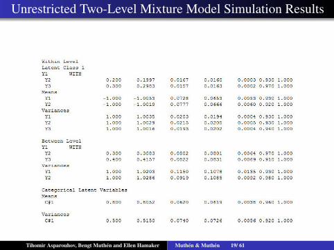
Unrestricted Two-Level Mixture Model Simulation Results
Tihomir Asparouhov, Bengt Muthen and Ellen Hamaker Muthen & Muthen 19/ 61
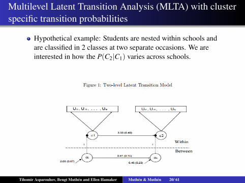
Multilevel Latent Transition Analysis (MLTA) with clusterspecific transition probabilities
Hypothetical example: Students are nested within schools andare classified in 2 classes at two separate occasions. We areinterested in how the P(C2|C1) varies across schools.
Tihomir Asparouhov, Bengt Muthen and Ellen Hamaker Muthen & Muthen 20/ 61

Multilevel Latent Transition Analysis (MLTA) with clusterspecific transition probabilities
The model that can be estimated in Mplus with ML
However γdcj does not really vary across clusters it is really γdcEven if we regress α2j on α1j (equivalent to correlation) we stillhave just 2 random effects for the joint distribution of two binarylatent class variables while the degrees of freedom is 3Current Mplus ML estimation P(C2|C1) does not fully varyacross clustersTihomir Asparouhov, Bengt Muthen and Ellen Hamaker Muthen & Muthen 21/ 61
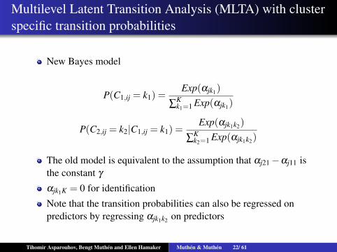
Multilevel Latent Transition Analysis (MLTA) with clusterspecific transition probabilities
New Bayes model
P(C1,ij = k1) =Exp(αjk1)
∑Kk1=1 Exp(αjk1)
P(C2,ij = k2|C1,ij = k1) =Exp(αjk1k2)
∑Kk2=1 Exp(αjk1k2)
The old model is equivalent to the assumption that αj21−αj11 isthe constant γ
αjk1K = 0 for identification
Note that the transition probabilities can also be regressed onpredictors by regressing αjk1k2 on predictors
Tihomir Asparouhov, Bengt Muthen and Ellen Hamaker Muthen & Muthen 22/ 61
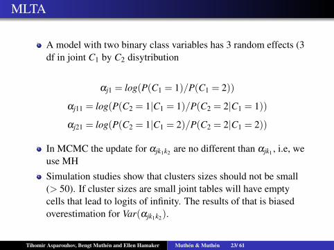
MLTA
A model with two binary class variables has 3 random effects (3df in joint C1 by C2 disytribution
αj1 = log(P(C1 = 1)/P(C1 = 2))
αj11 = log(P(C2 = 1|C1 = 1)/P(C2 = 2|C1 = 1))
αj21 = log(P(C2 = 1|C1 = 2)/P(C2 = 2|C1 = 2))
In MCMC the update for αjk1k2 are no different than αjk1 , i.e, weuse MH
Simulation studies show that clusters sizes should not be small(> 50). If cluster sizes are small joint tables will have emptycells that lead to logits of infinity. The results of that is biasedoverestimation for Var(αjk1k2).
Tihomir Asparouhov, Bengt Muthen and Ellen Hamaker Muthen & Muthen 23/ 61
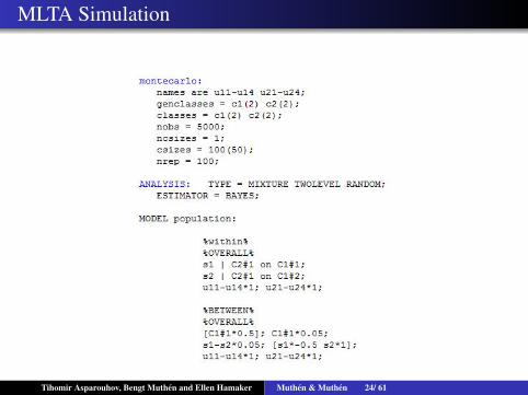
MLTA Simulation
Tihomir Asparouhov, Bengt Muthen and Ellen Hamaker Muthen & Muthen 24/ 61
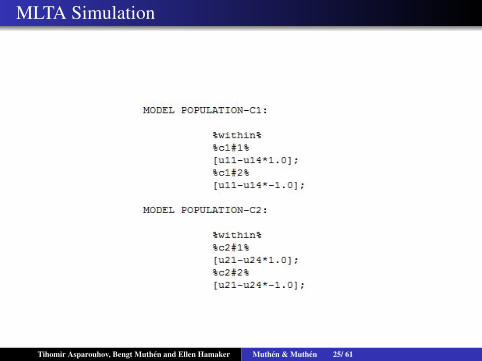
MLTA Simulation
Tihomir Asparouhov, Bengt Muthen and Ellen Hamaker Muthen & Muthen 25/ 61
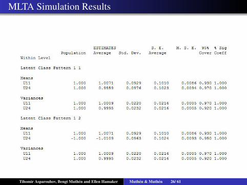
MLTA Simulation Results
Tihomir Asparouhov, Bengt Muthen and Ellen Hamaker Muthen & Muthen 26/ 61
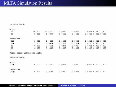
MLTA Simulation Results
Tihomir Asparouhov, Bengt Muthen and Ellen Hamaker Muthen & Muthen 27/ 61
Single Level LTA with Probability Parameterization
In single level the logits of transition probabilities are notrandom effects. They are non-random parameters.
Mplus has 3 different parameterizations for ML estimation ofLTA: logit, loglinear, probability
New Bayes estimation for LTA with probabilityparameterization: it allows for Lag=1 or Lag=2, P(C2|C1) orP(C3|C1,C2) just like ML
The model parameters are the probabilities directly P(C1) andP(C2|C1) and P(C3|C1,C2)
Easy MCMC implementation. P(C1) and P(C2|C1) andP(C3|C1,C2) have conjugate Dirichlet prior.
Tihomir Asparouhov, Bengt Muthen and Ellen Hamaker Muthen & Muthen 28/ 61
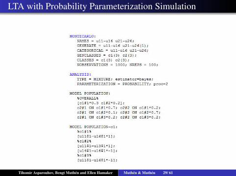
LTA with Probability Parameterization Simulation
Tihomir Asparouhov, Bengt Muthen and Ellen Hamaker Muthen & Muthen 29/ 61
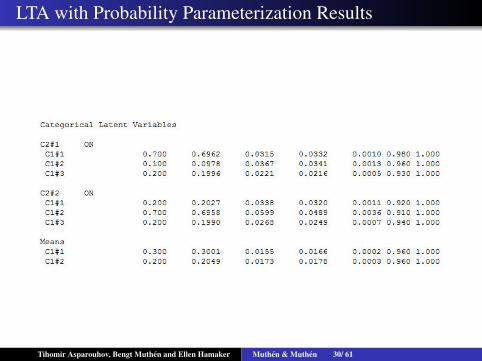
LTA with Probability Parameterization Results
Tihomir Asparouhov, Bengt Muthen and Ellen Hamaker Muthen & Muthen 30/ 61
Single Level Hidden Markov Models
Data is again intensive longitudinal. First we consider the singlelevel model, N=1. We discuss 3 models
Hidden Markov Model (HMM)Markov Switching Autoregressive (MSAR)Markov Switching Kalman Filter (MSKF)
DSEM allows for time series modeling for observed and latentcontinuous variables. DSEM Mixture does not allow autocorrelation for the latent categorical variable
In time series data it is not realistic to assume that St and St−1 areindependent, where St is the state/class variable at time t. On thecontrary. A realistic model will allow St and St−1 be highlycorrelated if the observations are taken very frequently.
Tihomir Asparouhov, Bengt Muthen and Ellen Hamaker Muthen & Muthen 31/ 61
Hidden Markov Models
The model has two parts: measurement part and Markovswitching part
The measurement part is like any other Mxiture model, it isdefined by P(Yt|St) where Yt is a vector of observed variablesand St is the latent class/state variable at time t
The Markov switching (regime switching) part is given byP(St|St−1). We use the same probability parametrization basedon Dirichlet conjugate priors that we used with two latent classvariables. The transition model Q = P(St|St−1) has K(K-1)probability parameters. The transition matrix is K by K but thecolumns add up to 1
Tihomir Asparouhov, Bengt Muthen and Ellen Hamaker Muthen & Muthen 32/ 61
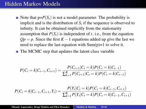
Hidden Markov Models
Note that p=P(St) is not a model parameter. The probability isimplicit and is the distribution of St if the sequence is observed toinfinity. It can be obtained implicitly from the stationarityassumption that P(St) is independent of t. i.e., from the equationQp = p. Since the first K−1 equations added up give the last weneed to replace the last equation with Sum(p)=1 to solve it.
The MCMC step that updates the latent class variable
P(Ct = k|Ct−1,Ct+1) =P(Ct+1|Ct = k)P(Ct = k|Ct−1)
∑Kk=1 P(Ct+1|Ct = k)P(Ct = k|Ct−1)
P(Ct = k|Ct−1,Ct+1,Yt) =P(Yt|Ct = k)P(Ct = k|Ct−1,Ct+1)
∑Kk=1 P(Yt|Ct = k)P(Ct = k|Ct−1,Ct+1)
Tihomir Asparouhov, Bengt Muthen and Ellen Hamaker Muthen & Muthen 33/ 61
Hidden Markov Models
Ct=0 is treated as an auxiliary parameter
Ct=0 can be given a prior
Mplus provides an automatic prior option. The prior is updatedin the first 100 MCMC iteration which are consequentlydiscarded and the prior is set to be the current sample distributionCt. This is the default.
If the length of the time series is long enough that prior does notmatter
Tihomir Asparouhov, Bengt Muthen and Ellen Hamaker Muthen & Muthen 34/ 61
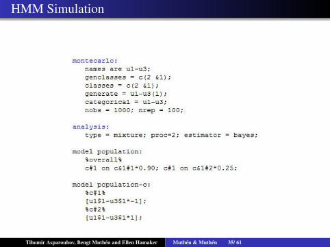
HMM Simulation
Tihomir Asparouhov, Bengt Muthen and Ellen Hamaker Muthen & Muthen 35/ 61
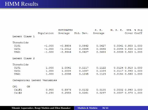
HMM Results
Tihomir Asparouhov, Bengt Muthen and Ellen Hamaker Muthen & Muthen 36/ 61
Combining HMM and DSEM
By combing HMM and DSEM we obtains a general model thatincludes time series for the latent class variable as well as factorsand observed variables
Markov Switching Autoregressive (MSAR) is simply thecombination of Mixture-AR and HMM
Markov Switching Kalman Filter (MSKF) is simply thecombination of Mixture-Kalman Filter and HMM
Tihomir Asparouhov, Bengt Muthen and Ellen Hamaker Muthen & Muthen 37/ 61
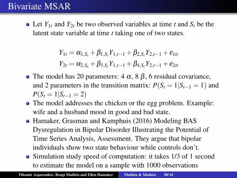
Bivariate MSAR
Let Y1t and Y2t be two observed variables at time t and St be thelatent state variable at time t taking one of two states.
Y1t = α1,St +β1,St Y1,t−1 +β2,St Y2,t−1 + ε1it
Y2t = α2,St +β3,St Y1,t−1 +β4,St Y2,t−1 + ε2it
The model has 20 parameters: 4 α , 8 β , 6 residual covariance,and 2 parameters in the transition matrix: P(St = 1|St−1 = 1) andP(St = 1|St−1 = 2)The model addresses the chicken or the egg problem. Example:wife and a husband mood in good and bad state.Hamaker, Grasman and Kamphuis (2016) Modeling BASDysregulation in Bipolar Disorder Illustrating the Potential ofTime Series Analysis, Assessment. They argue that bipolarindividuals show two state behaviour while controls don’t.Simulation study speed of computation: it takes 1/3 of 1 secondto estimate the model on a sample with 1000 observations
Tihomir Asparouhov, Bengt Muthen and Ellen Hamaker Muthen & Muthen 38/ 61
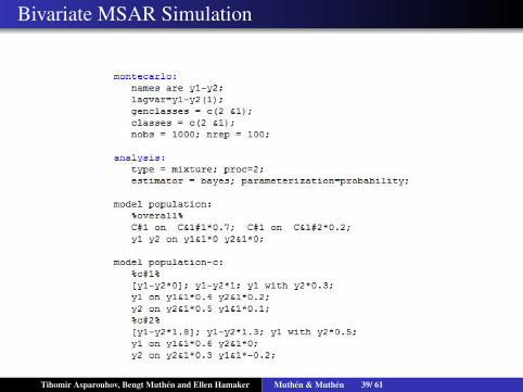
Bivariate MSAR Simulation
Tihomir Asparouhov, Bengt Muthen and Ellen Hamaker Muthen & Muthen 39/ 61
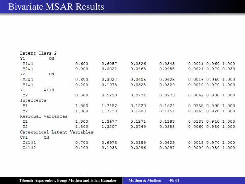
Bivariate MSAR Results
Tihomir Asparouhov, Bengt Muthen and Ellen Hamaker Muthen & Muthen 40/ 61
Markov Switching Kalman Filter (MSKF)
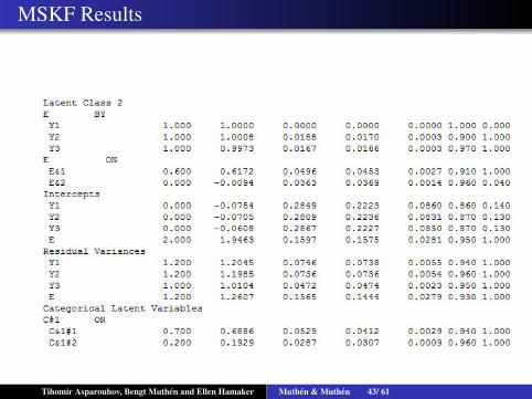
Three factor indicators Yjt measuring a factor ηt. St is a two statecategorical latent variable.We estimate a hidden Markov model for St, i.e.,P(St = 1|St−1 = 1) and P(St = 1|St−1 = 2) are probabilityparameters independent of t.For j=1,2,3
Yjt = νj +λjηt + εjt
ηt = αSt +β1,St ηt−1 +β2,St ηt−2 +ξt
MSAR(2) model for the factorFor identification purposes α1 = 0 and λ1 = 1 (this sets the scaleof the latent variable to be the same as the first indicator, whichis probably a better parameterization than fixing the variance ofthe factor to 1?)
Tihomir Asparouhov, Bengt Muthen and Ellen Hamaker Muthen & Muthen 41/ 61

MSKF Simulation
Tihomir Asparouhov, Bengt Muthen and Ellen Hamaker Muthen & Muthen 42/ 61
MSKF Results
Tihomir Asparouhov, Bengt Muthen and Ellen Hamaker Muthen & Muthen 43/ 61
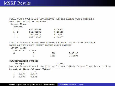
MSKF Results
Tihomir Asparouhov, Bengt Muthen and Ellen Hamaker Muthen & Muthen 44/ 61
MSKF Analysis of Results
Small bias in the means. What to do? I left this unanswered onpurpose to make the point. Possible potential causes
Model poorly identified: Not enough parameters differ acrossclass? Simplify model by holding parameter equal to improveidentification. Parameters that are not significantly different andmake sense can be constrained to be equal. Loadings notsignificantly different from 1 fix to 1.
Not enough sample size to get to bias of zero. Increase samplesize. Simplify model. Run simulations with bigger sample. Notethat Entropy remains the same as sample increases
Not enough MCMC iterations. Run with more iterations. Look atthe traceplot of the offending parameters to evaluate convergence
Label switching in Mixtures? I have not seen this happen yet. Ithink it it very rare because of the Markov regimeswitching/smoothing
Tihomir Asparouhov, Bengt Muthen and Ellen Hamaker Muthen & Muthen 45/ 61
MSKF Analysis of Results
Add informative priors to improve identifiability if the model.
Maybe entropy is too low?
In smaller sample size situations the number of regime switchingevents could be low if the state is stable - not enough to build themodel. Recall that we use P(Ct = 1|Ct−1 = 2) andP(Ct = 2|Ct−1 = 1) to figure out Ct distribution. If there are veryfew switch events accurate stable estimates are probablyunrealistic.
Other things I don’t know about
These methods are new and are the cutting edge of methodology.Not using simulation studies in parallel to a real data estimationis irresponsible. Simulation studies not possible in Bugs. Theyare possible in Mplus because it is much faster.
Tihomir Asparouhov, Bengt Muthen and Ellen Hamaker Muthen & Muthen 46/ 61
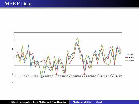
MSKF Data
Tihomir Asparouhov, Bengt Muthen and Ellen Hamaker Muthen & Muthen 47/ 61
MSKF Analysis
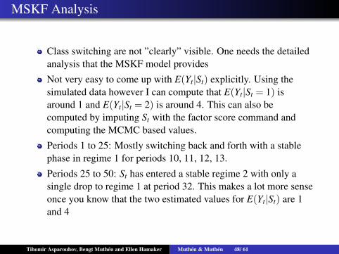
Class switching are not ”clearly” visible. One needs the detailedanalysis that the MSKF model provides
Not very easy to come up with E(Yt|St) explicitly. Using thesimulated data however I can compute that E(Yt|St = 1) isaround 1 and E(Yt|St = 2) is around 4. This can also becomputed by imputing St with the factor score command andcomputing the MCMC based values.
Periods 1 to 25: Mostly switching back and forth with a stablephase in regime 1 for periods 10, 11, 12, 13.
Periods 25 to 50: St has entered a stable regime 2 with only asingle drop to regime 1 at period 32. This makes a lot more senseonce you know that the two estimated values for E(Yt|St) are 1and 4
Tihomir Asparouhov, Bengt Muthen and Ellen Hamaker Muthen & Muthen 48/ 61
Two level models
Not really two-level models. These are intensive longitudinalmodels: multiple observations nested within clusters.
This methodology more suitable for social sciences than the caseof N=1
Dynamic Latent Class Analysis (DLCA)
Multilevel Markov Switching Autoregressive Models(MMSAR)
Multilevel Markov Switching Kalman Filter Models (MMSKF)
Tihomir Asparouhov, Bengt Muthen and Ellen Hamaker Muthen & Muthen 49/ 61
Dynamic Latent Class Analysis
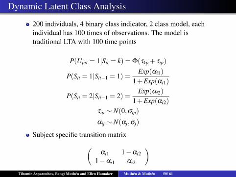
200 individuals, 4 binary class indicator, 2 class model, eachindividual has 100 times of observations. The model istraditional LTA with 100 time points
P(Upit = 1|Sit = k) = Φ(τkp + τip)
P(Sit = 1|Sit−1 = 1) =Exp(αi1)
1+Exp(αi1)
P(Sit = 2|Sit−1 = 2) =Exp(αi2)
1+Exp(αi2)
τip ∼ N(0,σip)
αij ∼ N(αj,σj)
Subject specific transition matrix(αi1 1−αi2
1−αi1 αi2
)Tihomir Asparouhov, Bengt Muthen and Ellen Hamaker Muthen & Muthen 50/ 61
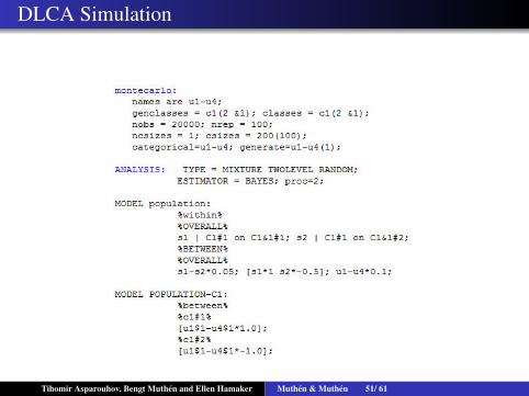
DLCA Simulation
Tihomir Asparouhov, Bengt Muthen and Ellen Hamaker Muthen & Muthen 51/ 61
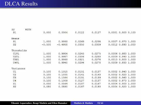
DLCA Results
Tihomir Asparouhov, Bengt Muthen and Ellen Hamaker Muthen & Muthen 52/ 61
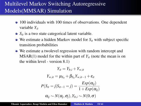
Multilevel Markov Switching AutoregressiveModels(MMSAR) Simulation
100 individuals with 100 times of observations. One dependentvariable Yit
Sit is a two state categorical latent variable.We estimate a hidden Markov model for Sit with subject specifictransition probabilitiesWe estimate a twolevel regression with random intercept andMSAR(1) model for the within part of Yit (note the mean is onthe within level - version 8.1)
Yit = Yb,i +Yw,it
Yw,it = µSit +βSit Yw,it−1 + εit
P(Sit = j|Sit−1 = j) =Exp(αij)
1+Exp(αij)
αij ∼ N(αj,σj),Yb,i ∼ N(0,σ)
Tihomir Asparouhov, Bengt Muthen and Ellen Hamaker Muthen & Muthen 53/ 61
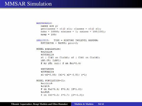
MMSAR Simulation
Tihomir Asparouhov, Bengt Muthen and Ellen Hamaker Muthen & Muthen 54/ 61
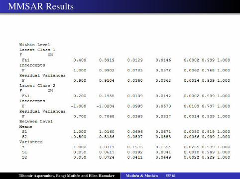
MMSAR Results
Tihomir Asparouhov, Bengt Muthen and Ellen Hamaker Muthen & Muthen 55/ 61
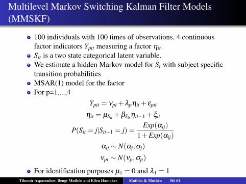
Multilevel Markov Switching Kalman Filter Models(MMSKF)
100 individuals with 100 times of observations, 4 continuousfactor indicators Ypit measuring a factor ηit.Sit is a two state categorical latent variable.We estimate a hidden Markov model for St with subject specifictransition probabilitiesMSAR(1) model for the factorFor p=1,...,4
Ypit = νpi +λpηit + εpit
ηit = µSit +βSit ηit−1 +ξit
P(Sit = j|Sit−1 = j) =Exp(αij)
1+Exp(αij)
αij ∼ N(αj,σj)
νpi ∼ N(νp,σp)
For identification purposes µ1 = 0 and λ1 = 1Tihomir Asparouhov, Bengt Muthen and Ellen Hamaker Muthen & Muthen 56/ 61
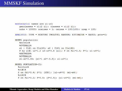
MMSKF Simulation
Tihomir Asparouhov, Bengt Muthen and Ellen Hamaker Muthen & Muthen 57/ 61
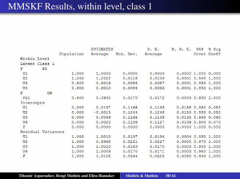
MMSKF Results, within level, class 1
Tihomir Asparouhov, Bengt Muthen and Ellen Hamaker Muthen & Muthen 58/ 61
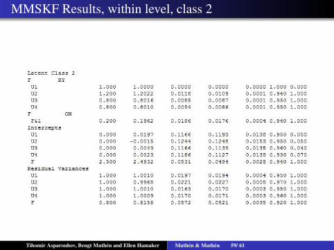
MMSKF Results, within level, class 2
Tihomir Asparouhov, Bengt Muthen and Ellen Hamaker Muthen & Muthen 59/ 61

MMSKF Results, between level
Tihomir Asparouhov, Bengt Muthen and Ellen Hamaker Muthen & Muthen 60/ 61
Issues
Determine the number of classes: ignore time series and usestandard methods
Starting values: maybe coming soon, not as big issue for Bayesas it is for ML due to MCMC naturally goes through manystarting values
Comparing models: maybe coming soon DIC, model test, newPPP methods, other new methods
Multiple solutions: We get a lot of multiple solutions with ML.Does that happen with Bayes too? Using different startingvalues? This is an issue even without time-series.
Label switching - hopefully not much of a problem due toMarkov smoothing
Tihomir Asparouhov, Bengt Muthen and Ellen Hamaker Muthen & Muthen 61/ 61