laser communications for lisa and the university of
TRANSCRIPT

LASER COMMUNICATIONS FOR LISA AND THE UNIVERSITY OF FLORIDA LISAINTERFEROMETRY SIMULATOR
By
DYLAN SWEENEY
A DISSERTATION PRESENTED TO THE GRADUATE SCHOOLOF THE UNIVERSITY OF FLORIDA IN PARTIAL FULFILLMENT
OF THE REQUIREMENTS FOR THE DEGREE OFDOCTOR OF PHILOSOPHY
UNIVERSITY OF FLORIDA
2012
c⃝ 2012 Dylan Sweeney
2

I dedicate this work to my wife, Sandra Londono, without you nothing I have achievedwould be possible. You gave me the strength and confidence I needed to finish this
thesis. You are my inspiration and you give meaning to everything I do.
I also dedicate this work to our son, Nicolas Sweeney. May you find everything you seekin life.
3

ACKNOWLEDGMENTS
I owe a debt of gratitude to all of the people who have assisted me in my work.
Thanks to Guido Mueller, my thesis advisor, for providing the expertise to guide my
research, the laboratory to work in, and prompt and helpful feedback on my progress.
Thanks to my fellow graduate students Alix Preston, Yinan Yu, Shawn Mitryk, Johannes
Eichholz, Aaron Spector, and Darsa Donelan, who have been excellent co workers.
Special thanks to Shawn Mitryk whose help using our digital signal processing
hardware was invaluable. Thanks to the post-docs in the lab Vinzenz Wand, Jose
Sanjuan Munoz, and Syed Azer Reza who were always available to help me. Thanks
to the undergraduate students Justin Cohen and Amanda Cordes, who assisted in the
development of my experimental set up.
4
TABLE OF CONTENTS
page
ACKNOWLEDGMENTS . . . . . . . . . . . . . . . . . . . . . . . . . . . . . . . . . . 4
LIST OF FIGURES . . . . . . . . . . . . . . . . . . . . . . . . . . . . . . . . . . . . . 8
ABSTRACT . . . . . . . . . . . . . . . . . . . . . . . . . . . . . . . . . . . . . . . . . 11
CHAPTER
1 BACKGROUND: GENERAL RELATIVITY AND GRAVITATIONAL WAVES . . . 12
1.1 General Relativity . . . . . . . . . . . . . . . . . . . . . . . . . . . . . . . 121.2 Gravitational Waves . . . . . . . . . . . . . . . . . . . . . . . . . . . . . . 14
1.2.1 Detection . . . . . . . . . . . . . . . . . . . . . . . . . . . . . . . . 151.2.2 Generation . . . . . . . . . . . . . . . . . . . . . . . . . . . . . . . 17
1.3 Gravitational Waves Sources . . . . . . . . . . . . . . . . . . . . . . . . . 181.3.1 Binary Systems . . . . . . . . . . . . . . . . . . . . . . . . . . . . . 181.3.2 Extreme Mass Ratio Inspirals . . . . . . . . . . . . . . . . . . . . . 201.3.3 Supernova . . . . . . . . . . . . . . . . . . . . . . . . . . . . . . . . 201.3.4 Rotating Neutron Stars . . . . . . . . . . . . . . . . . . . . . . . . . 211.3.5 Stochastic Background . . . . . . . . . . . . . . . . . . . . . . . . . 22
1.4 Gravitational Wave Detectors . . . . . . . . . . . . . . . . . . . . . . . . . 221.4.1 Resonant Mass Detectors . . . . . . . . . . . . . . . . . . . . . . . 221.4.2 Pulsar Timing . . . . . . . . . . . . . . . . . . . . . . . . . . . . . . 231.4.3 Ground Based Laser Interferometers . . . . . . . . . . . . . . . . . 231.4.4 Space Based Laser Interferometers . . . . . . . . . . . . . . . . . 27
2 THE LASER INTERFEROMETRY SPACE ANTENNA (LISA) . . . . . . . . . . 28
2.1 Disturbance Reduction System . . . . . . . . . . . . . . . . . . . . . . . . 282.2 Interferometric Measurement System . . . . . . . . . . . . . . . . . . . . 30
2.2.1 IMS Overview . . . . . . . . . . . . . . . . . . . . . . . . . . . . . . 302.2.2 Noise Requirement . . . . . . . . . . . . . . . . . . . . . . . . . . . 302.2.3 Heterodyne Interferometry . . . . . . . . . . . . . . . . . . . . . . . 322.2.4 LISA Sensor Signals . . . . . . . . . . . . . . . . . . . . . . . . . . 332.2.5 Laser Noise Removal . . . . . . . . . . . . . . . . . . . . . . . . . 342.2.6 Time Delay Interferometry . . . . . . . . . . . . . . . . . . . . . . . 352.2.7 Phasemeters . . . . . . . . . . . . . . . . . . . . . . . . . . . . . . 37
2.3 Laser Communication System and Requirements . . . . . . . . . . . . . . 382.3.1 Clock Noise Transfers . . . . . . . . . . . . . . . . . . . . . . . . . 39
2.3.1.1 Electro-Optic Modulators . . . . . . . . . . . . . . . . . . 392.3.1.2 Frequency Synthesizers . . . . . . . . . . . . . . . . . . . 402.3.1.3 TDI with Clock Noise Removal . . . . . . . . . . . . . . . 412.3.1.4 Clock Transfer Chain Noise Requirement . . . . . . . . . 42
2.3.2 Laser Ranging . . . . . . . . . . . . . . . . . . . . . . . . . . . . . 43
5

3 THE UNIVERSITY OF FLORIDA LISA INTERFEROMETRY SIMULATOR . . . 49
3.1 UFLIS Concept . . . . . . . . . . . . . . . . . . . . . . . . . . . . . . . . . 493.2 Laser Bench Top Set-Up . . . . . . . . . . . . . . . . . . . . . . . . . . . . 503.3 Prestabilization . . . . . . . . . . . . . . . . . . . . . . . . . . . . . . . . . 523.4 Electrical Components . . . . . . . . . . . . . . . . . . . . . . . . . . . . . 523.5 Digital Signal Processing Hadware . . . . . . . . . . . . . . . . . . . . . . 533.6 Phasemeter . . . . . . . . . . . . . . . . . . . . . . . . . . . . . . . . . . . 543.7 Electronic Phase Delay Unit . . . . . . . . . . . . . . . . . . . . . . . . . . 563.8 Previous Experiments with UFLIS . . . . . . . . . . . . . . . . . . . . . . 563.9 Goals of this Work . . . . . . . . . . . . . . . . . . . . . . . . . . . . . . . 58
4 VERIFICATION OF INTER SPACE CRAFT CLOCK TRANSFER . . . . . . . . 59
4.1 Tests of Frequency Synthesizers . . . . . . . . . . . . . . . . . . . . . . . 594.1.1 Stanford Clocks . . . . . . . . . . . . . . . . . . . . . . . . . . . . . 594.1.2 Custom Phase Lock Loop . . . . . . . . . . . . . . . . . . . . . . . 604.1.3 Rupptronik Frequency Synthesizers . . . . . . . . . . . . . . . . . 614.1.4 Results . . . . . . . . . . . . . . . . . . . . . . . . . . . . . . . . . 62
4.2 Tests of Electro-Optic Modulators . . . . . . . . . . . . . . . . . . . . . . . 634.2.1 MHz Test . . . . . . . . . . . . . . . . . . . . . . . . . . . . . . . . 644.2.2 GHz Test . . . . . . . . . . . . . . . . . . . . . . . . . . . . . . . . 65
4.3 Frequency Synthesizer and EOM Combination . . . . . . . . . . . . . . . 684.4 Electronic Test of Clock Noise Transfer . . . . . . . . . . . . . . . . . . . . 70
5 DEVELOPMENT OF PSEUDO-RANDOM NOISE CODE RANGING . . . . . . 73
5.1 Delay-Locked Loop (DLL) Design . . . . . . . . . . . . . . . . . . . . . . . 735.1.1 Phasemeter Transfer Function . . . . . . . . . . . . . . . . . . . . . 735.1.2 Filtering the Double Frequency Term . . . . . . . . . . . . . . . . . 745.1.3 Linearized Delay-Locked Loop Model . . . . . . . . . . . . . . . . . 825.1.4 Choice of Filter Parameters . . . . . . . . . . . . . . . . . . . . . . 845.1.5 Noise Term Analysis . . . . . . . . . . . . . . . . . . . . . . . . . . 86
5.1.5.1 Phasemeter Out of Band Noise . . . . . . . . . . . . . . . 875.1.5.2 Local PRN code Interference . . . . . . . . . . . . . . . . 88
5.1.6 Rounding of Tracking Code Delay . . . . . . . . . . . . . . . . . . . 905.2 Delay-Locked Loop Simulations . . . . . . . . . . . . . . . . . . . . . . . . 915.3 Optical Delay-Locked Loop Tests . . . . . . . . . . . . . . . . . . . . . . . 95
5.3.1 Tracking PRN Code Generated with Local Clock . . . . . . . . . . 965.3.2 Tracking PRN Code Generated With a Separate Clock . . . . . . . 995.3.3 Delay-Locked Loop Tracking With Interfering PRN Code . . . . . . 103
6 ELECTRONIC TEST OF TDI WITH PRN RANGING . . . . . . . . . . . . . . . 108
6

7 FUTURE INTEGRATION OF UFLIS AND LASER COMMUNICATION . . . . . 112
7.1 PRN Ranging and the Phasemeter Delay Unit . . . . . . . . . . . . . . . . 1127.2 Clock Noise Transfers and UFLIS . . . . . . . . . . . . . . . . . . . . . . . 113
8 CONCLUSION . . . . . . . . . . . . . . . . . . . . . . . . . . . . . . . . . . . . 117
REFERENCES . . . . . . . . . . . . . . . . . . . . . . . . . . . . . . . . . . . . . . . 120
BIOGRAPHICAL SKETCH . . . . . . . . . . . . . . . . . . . . . . . . . . . . . . . . 124
7

LIST OF FIGURES
Figure page
1-1 Basic and advanced Michelson interferometers . . . . . . . . . . . . . . . . . . 24
2-1 The orbit of the three LISA SC . . . . . . . . . . . . . . . . . . . . . . . . . . . 29
2-2 Diagram of the LISA satellites . . . . . . . . . . . . . . . . . . . . . . . . . . . . 31
2-3 A simplified version of the layout of the LISA optical bench . . . . . . . . . . . . 35
2-4 The three step approach to canceling the intrinsic laser phase noise in LISA . . 36
2-5 An IQ tracking phasemeter . . . . . . . . . . . . . . . . . . . . . . . . . . . . . 38
2-6 Simplified model of LISA that UFLIS is based on . . . . . . . . . . . . . . . . . 43
2-7 The laser modulation scheme . . . . . . . . . . . . . . . . . . . . . . . . . . . . 44
2-8 The PRN code and the Manchester encoding scheme . . . . . . . . . . . . . . 45
2-9 Forming the PRN error signal . . . . . . . . . . . . . . . . . . . . . . . . . . . . 46
2-10 The delay lock loop architecture . . . . . . . . . . . . . . . . . . . . . . . . . . 46
3-1 How the EPD unit models the long travel times of the LISA arms . . . . . . . . 50
3-2 The previous set up of the laser bench top for UFLIS . . . . . . . . . . . . . . . 51
3-3 The current set up of the laser bench top for UFLIS . . . . . . . . . . . . . . . . 51
3-4 The formation of optical beat notes in the current UFLIS set up . . . . . . . . . 52
3-5 The electronic portion of UFLIS . . . . . . . . . . . . . . . . . . . . . . . . . . . 53
3-6 The digital signal processing system . . . . . . . . . . . . . . . . . . . . . . . . 54
3-7 Spectral results of two measurements of the UFLIS phasemeter system . . . . 55
3-8 Spectral results of a test of the sample and hold EPD unit . . . . . . . . . . . . 57
4-1 Experimental set up to test the frequency synthesizers . . . . . . . . . . . . . . 60
4-2 The PLL used to lock the 2 GHz VCO to a 10 MHz signal . . . . . . . . . . . . 61
4-3 Set up and spectral results of a test of frequency down converters . . . . . . . 62
4-4 Spectral results of the three frequency up-conversion measurements . . . . . . 63
4-5 The experimental set up for the test of the EOM’s phase stability at 5 MHz . . . 65
4-6 Spectral results of the EOM’s phase stability at 5 MHz . . . . . . . . . . . . . . 66
8

4-7 The experimental set up for the test of the EOM’s phase stability at 2 GHz . . . 67
4-8 Spectral results of the EOM’s phase stability at 2 GHz . . . . . . . . . . . . . . 67
4-9 Combined test of both the frequency synthesizers and the EOMs . . . . . . . . 69
4-10 Linear spectral density of combined synthesizer and EOM measurement . . . 69
4-11 The set-up for the electronic test of the clock noise transfer concept using frequencysynthesizers . . . . . . . . . . . . . . . . . . . . . . . . . . . . . . . . . . . . . 72
4-12 Linear spectral density of the results of the electronic test of the clock noisetransfer concept using frequency synthesizers . . . . . . . . . . . . . . . . . . 72
5-1 Diagram of the LISA phasemeter and Delay-Locked Loop . . . . . . . . . . . . 74
5-2 Phasemeter with filter to remove the 2ν term. . . . . . . . . . . . . . . . . . . . 77
5-3 The PRN code after demodulation from the carrier with and without the 2ν filter 78
5-4 Error signals with and without the 2ν filter at beat notes of 1, 2, and 2.5 MHz . 79
5-5 Error signals with and without the 2ν filter at beat note of 3, 5, and 10 MHz . . 80
5-6 Error signals with and without the 2ν filter at beat notes of 13.5, 15, and 20 MHz 81
5-7 The Delay-Locked Loop . . . . . . . . . . . . . . . . . . . . . . . . . . . . . . . 83
5-8 Error signal formed with early-late correlation of Manchester encoded PRN. . . 84
5-9 Linearized version of the Delay-Locked Loop . . . . . . . . . . . . . . . . . . . 85
5-10 Digital implementation of a single pole low pass filter. . . . . . . . . . . . . . . 86
5-11 Simulated tracking signal error caused by interfering PRN code. . . . . . . . . 89
5-12 Possible relative positions between the incoming PRN code and the trackingcode. . . . . . . . . . . . . . . . . . . . . . . . . . . . . . . . . . . . . . . . . . 92
5-13 Spectral results of the DLL tracking simulation with noise at 1 µcycles/√Hz . . 93
5-14 Spectral results of the DLL tracking simulation with noise at 10 µcycles/√Hz . . 94
5-15 Optical set up of the PRN ranging experiments. . . . . . . . . . . . . . . . . . . 97
5-16 Power spectral densities of beat notes used in optical DLL tests. . . . . . . . . 98
5-17 Plot of measured pseudo ranges with 1 µcycle/√Hz noise while tracking PRN
generated on local clock . . . . . . . . . . . . . . . . . . . . . . . . . . . . . . . 98
5-18 Spectral results of measured pseudo ranges with 1 µcycle/√Hz noise while
tracking PRN generated on local clock . . . . . . . . . . . . . . . . . . . . . . . 99
9
5-19 Plot of measured pseudo ranges with 10 µcycle/√Hz noise while tracking PRN
generated on local clock . . . . . . . . . . . . . . . . . . . . . . . . . . . . . . . 100
5-20 Spectral results of measured pseudo ranges with 10 µcycle/√Hz noise while
tracking PRN generated on local clock . . . . . . . . . . . . . . . . . . . . . . . 101
5-21 Plots of measured pseudo ranges with 1 µcycle/√Hz noise while tracking PRN
generated on a separate clock . . . . . . . . . . . . . . . . . . . . . . . . . . . 101
5-22 Spectral results of measured pseudo ranges with 1 µcycle/√Hz noise while
tracking PRN generated on la separate clock . . . . . . . . . . . . . . . . . . . 102
5-23 Plot of measured pseudo range with 10 µcycle/√Hz noise while tracking a
PRN code generated on a separate clock . . . . . . . . . . . . . . . . . . . . . 102
5-24 Long term tracking of PRN code generated on a separate clock with 10 µcycle/√Hz
noise . . . . . . . . . . . . . . . . . . . . . . . . . . . . . . . . . . . . . . . . . 104
5-25 Spectral results of long term tracking of PRN code generated on a separateclock with 10 µcycle/
√Hz noise . . . . . . . . . . . . . . . . . . . . . . . . . . . 105
5-26 Time series of DLL tracking with interfering code at a clock offset of 2.3 Hz . . 105
5-27 Spectral results of DLL tracking with interfering code at clock offset of 2.3 Hz . 106
5-28 Time series of DLL tracking with interfering code at clock offset of 52.3 Hz . . . 106
5-29 Spectral results of DLL tracking with interfering code at clock offset of 52.3 Hz 107
6-1 Experimental set up of the electronic test of TDI with PRN ranging . . . . . . . 109
6-2 Spectral results of the electronic test of TDI with PRN ranging . . . . . . . . . . 110
7-1 Modifications to the phasemeter EPD unit to include PRN code delays. . . . . 113
7-2 Spectral results of the error in the PRN code timing using the phasemeter EPDunit . . . . . . . . . . . . . . . . . . . . . . . . . . . . . . . . . . . . . . . . . . 114
7-3 Preliminary test of UFLIS with clock noise transfers . . . . . . . . . . . . . . . . 116
10

Abstract of Dissertation Presented to the Graduate Schoolof the University of Florida in Partial Fulfillment of theRequirements for the Degree of Doctor of Philosophy
LASER COMMUNICATIONS FOR LISA AND THE UNIVERSITY OF FLORIDA LISAINTERFEROMETRY SIMULATOR
By
Dylan Sweeney
December 2012
Chair: Guido MuellerMajor: Physics
The Laser Interferometer Space Antenna (LISA) is a proposed joint space based
gravitational wave detector between the National Aeronautics and Space Administration
(NASA) and the European Space Agency (ESA). The LISA mission uses laser
interferometry to measure fluctuations in the path length between three spacecraft
caused by gravitational waves. LISA is designed to be sensitive to gravitational waves in
the frequency band 30 µ Hz to 1 Hz complementing ground based detectors which are
sensitive at higher frequencies. There are many components to the LISA mission, all of
which must be tested prior to launch. One such component is the laser communication
subsystem which is used to transfer clock signals, measure the range, and to share
recorded data between the spacecraft using the laser links between the spacecraft.
Researchers at the University of Florida have constructed a simulator of the LISA
interferometry (UFLIS). This simulator has been used to verify the efficacy of several
LISA technologies including time delay interferometry and arm locking. This dissertation
describes work done at the University of Florida to test individual components of the
laser communication subsystem and to integrate them into UFLIS.
11

CHAPTER 1BACKGROUND: GENERAL RELATIVITY AND GRAVITATIONAL WAVES
1.1 General Relativity
The principle of Galilean relativity, that all uniform motion is relative, is a key feature
of Newtonian mechanics and was once thought to be a universal principle. However, the
laws of classical electrodynamics, which were discovered through experiments, were
not invariant under a Galilean transformation of coordinates from one inertial frame to
another. In 1905 Einstein published his special theory of relativity. By requiring that
uniform motion be relative and that the speed of light be the same in all inertial frames,
Einstein boldly claimed that all the laws of physics should be invariant under Lorentz
transformations, not Galilean transformations. Interestingly special relativity implies
that the distance between points and the time between events are not the same for all
observers. Instead the spacetime interval
�s2 = −�t2 + �x2 + �y 2 + �z2 (1–1)
is the same for all observers in inertial reference frames in special relativity (in this
chapter we will take units with c = G = 1). Since this quantity contains both time and
space, special relativity is formulated in terms of a spacetime geometry. In this geometry
events in spacetime are labeled by four-vectors
xµ = (t, x , y , z) (1–2)
This geometry can be characterized by a metric tensor which determines how the
invariant interval is calculated. In special relativity the metric is
ηµν =
−1 0 0 0
0 1 0 0
0 0 1 0
0 0 0 1
(1–3)
12

The spacetime interval can be calculated as
�s2 = ηµνxµxν = xµx
ν (1–4)
using the Einstein summation convention in which repeated indices are summed
(aµbµ = �3µ=0aµb
µ). This is further shortened by lowering an index by (aµ = ηµνaν). Greek
letters are taken to be the combined time and spatial indices 0-3, while Latin letters are
taken to be just the spatial indices 1-3.
While the laws of classical electrodynamics are invariant under Lorentz transformations,
Newton’s law of gravity is not. In 1917 Einstein published his general theory of relativity
which replaced Newtonian gravity with a theory consistent with special relativity. In
general relativity gravity is not a force acting on masses, but the result of the curvature
of spacetime due to the presence of matter/energy. This curvature is expressed by the
spacetime metric which, in general relativity, is a dynamical variable changing over both
space and time. In general relativity ηµν is replaced with gµν and the spacetime interval
must be calculated as
�s =
∫gµνdx
µdxν (1–5)
because gµν itself depends on the coordinates.
Given a metric gµν , the motion of matter is given by
d2xµ
dτ 2+ �µ
νρ
dxν
dτ
dxρ
dτ= 0 (1–6)
This is called the geodesic equation. �µνρ is the Chrisoffel symbol and is defined by
�µνρ ≡1
2(−∂µgνρ + ∂ρgνµ + ∂νgµρ) (1–7)
The metric is given by the Einstein field equations
Rµν −1
2gµνR = 8πGTµν (1–8)
13

Rµν is the Ricci curvature tensor and is given by
Rµν = ∂ρ�ρµν − ∂ν�
ρµρ + �ρ
µν�σρσ + �σ
µρ�ρνσ (1–9)
R is the Ricci Scalar and is given by contracting both indices of the Ricci curvature
tensor. The Ricci curvature tensor is a measure of the curvature of the geometry.
It represents the curvature of spacetime as a measure of the tendency of matter to
converge or diverge over time.
Tµν is the energy momentum tensor, it is a measure of the flux of the µ component
of the four momentum across a unit area of the xν = constant surface. Therefore the
energy momentum tensor has components corresponding to energy density (T00),
momentum density(T0i ), energy flux(Ti0), shear stress(Tij i = j), and pressure(Tii ). One
can think of the geodesic equation, which describes the motion of matter in a spacetime
metric, as analogous to the Lorentz force law, which describes the motion of charged
particles in electric and magnetic fields. Likewise one can think of the Einstein field
equations, which describe the spacetime metric in the presence of matter/energy, as
being analogous to Maxwell’s equations, which describe the electric and magnetic fields
in the presence of charged particles.
1.2 Gravitational Waves
In classical electrodynamics Maxwell’s equations lead directly to wave solutions
of the electric and magnetic fields in free space where there are no sources. Since
Einstein’s equations are nonlinear they must first be linearized in order to get wave
solutions. To do so it is assumed that the spacetime metric only contains small
perturbations to flat spacetime
gµν = ηµν + hµν (1–10)
14
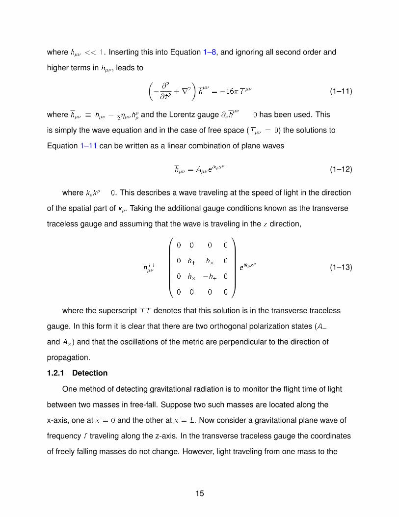
where hµν << 1. Inserting this into Equation 1–8, and ignoring all second order and
higher terms in hµν , leads to (− ∂2
∂t2+∇2
)hµν
= −16πT µν (1–11)
where hµν ≡ hµν − 12ηµνh
ρρ and the Lorentz gauge ∂νh
µν= 0 has been used. This
is simply the wave equation and in the case of free space (Tµν = 0) the solutions to
Equation 1–11 can be written as a linear combination of plane waves
hµν = Aµνeikρx
ρ
(1–12)
where kρkρ = 0. This describes a wave traveling at the speed of light in the direction
of the spatial part of kρ. Taking the additional gauge conditions known as the transverse
traceless gauge and assuming that the wave is traveling in the z direction,
hTTµν =
0 0 0 0
0 h+ h× 0
0 h× −h+ 0
0 0 0 0
e ikρx
ρ
(1–13)
where the superscript TT denotes that this solution is in the transverse traceless
gauge. In this form it is clear that there are two orthogonal polarization states (A+
and A×) and that the oscillations of the metric are perpendicular to the direction of
propagation.
1.2.1 Detection
One method of detecting gravitational radiation is to monitor the flight time of light
between two masses in free-fall. Suppose two such masses are located along the
x-axis, one at x = 0 and the other at x = L. Now consider a gravitational plane wave of
frequency f traveling along the z-axis. In the transverse traceless gauge the coordinates
of freely falling masses do not change. However, light traveling from one mass to the
15
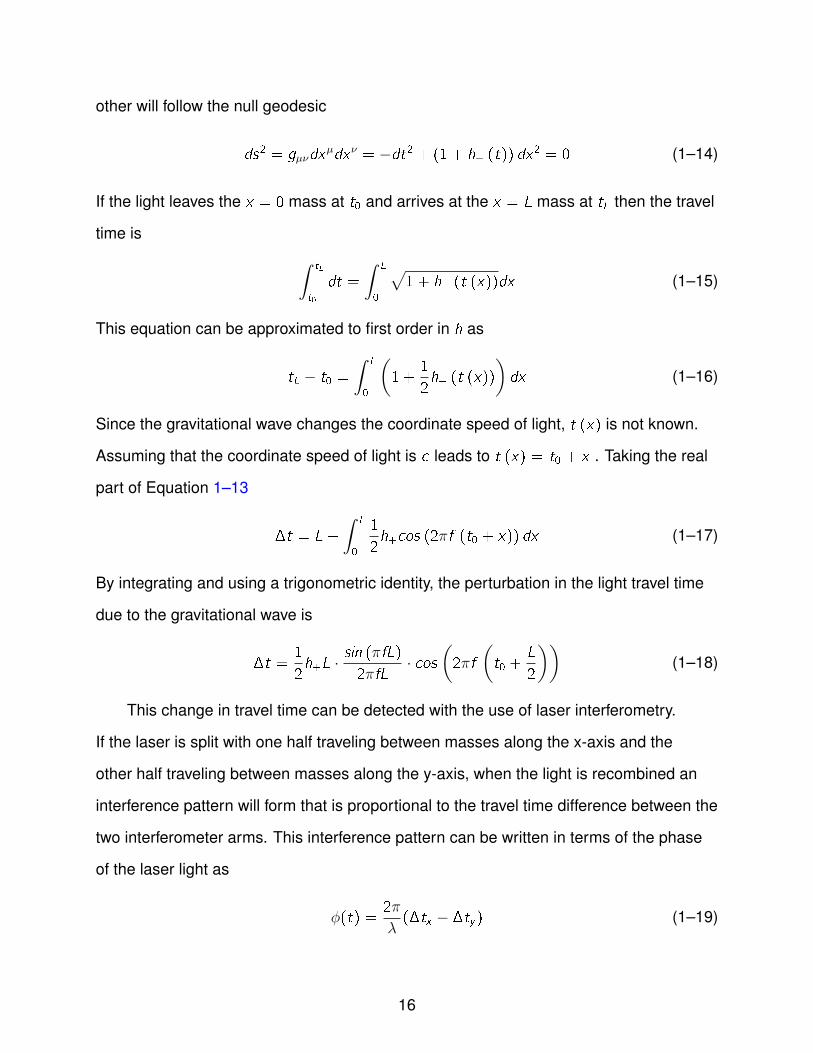
other will follow the null geodesic
ds2 = gµνdxµdxν = −dt2 + (1 + h+ (t)) dx2 = 0 (1–14)
If the light leaves the x = 0 mass at t0 and arrives at the x = L mass at tL then the travel
time is ∫ tL
t0
dt =
∫ L
0
√1 + h+ (t (x))dx (1–15)
This equation can be approximated to first order in h as
tL − t0 =
∫ L
0
(1 +
1
2h+ (t (x))
)dx (1–16)
Since the gravitational wave changes the coordinate speed of light, t (x) is not known.
Assuming that the coordinate speed of light is c leads to t (x) = t0 + x . Taking the real
part of Equation 1–13
�t = L+
∫ L
0
1
2h+cos (2πf (t0 + x)) dx (1–17)
By integrating and using a trigonometric identity, the perturbation in the light travel time
due to the gravitational wave is
�t =1
2h+L · sin (πfL)
2πfL· cos
(2πf
(t0 +
L
2
))(1–18)
This change in travel time can be detected with the use of laser interferometry.
If the laser is split with one half traveling between masses along the x-axis and the
other half traveling between masses along the y-axis, when the light is recombined an
interference pattern will form that is proportional to the travel time difference between the
two interferometer arms. This interference pattern can be written in terms of the phase
of the laser light as
ϕ(t) =2π
λ(�tx − �ty) (1–19)
16

where λ is the wavelength of the laser light. For the + polarization of a wave traveling
along the z-axis, the perturbations in the light travel time along the x and y axes will be
out of phase, causing them to add in Equation 1–19. This will lead to a modulation in the
laser phase at the frequency of the gravitational wave at an amplitude of
ϕ ≈ 2π
λh+L (1–20)
1.2.2 Generation
Using the retarded Green’s function and setting R2 = (x i − y i)(xi − yi) the general
solution to Equation 1–11 is
hµν(t, x i
)= 4
∫1
RTµν
(t − R, y i
)d3y (1–21)
where x i is the field position, y i is the source position, t is the time, and t − R is the
retarded time (the time it takes the gravitational signal to propagate from the source to
the field point). Assuming that the source of the gravitational wave is near the origin and
that the field is measured far away from the source, r 2 = x ixi >> y iyi , and assuming that
the source is traveling much slower than the speed of light, ddty i << 1, it can be shown
that the spatial components of hµν are given by
hjk(t, x i
)=
2
r
d2Ijk (t − r)
dt2(1–22)
where Ijk is the quadrupole moment of the source. The quadrupole moment is defined
as
Ijk (t) =
∫y jy kρd3y (1–23)
Equation 1–22 implies that in order to generate a gravitational wave an astrophysical
system must have non zero second derivative of the quadrupole moment. This means
that the system must be accelerating in a non-spherically symmetric way. Such systems
are discussed in the next section.
17
1.3 Gravitational Waves Sources
There are several different types of astrophysical sources that are predicted to
emit gravitational waves that will be detectable by current and future gravitational wave
detectors. Among them are binaries of compact objects (white dwarfs, neutron stars, or
black holes), extreme mass ratio inspirals, supernova collapse, spinning neutron stars,
and the stochastic background of gravitational waves left over from the big bang.
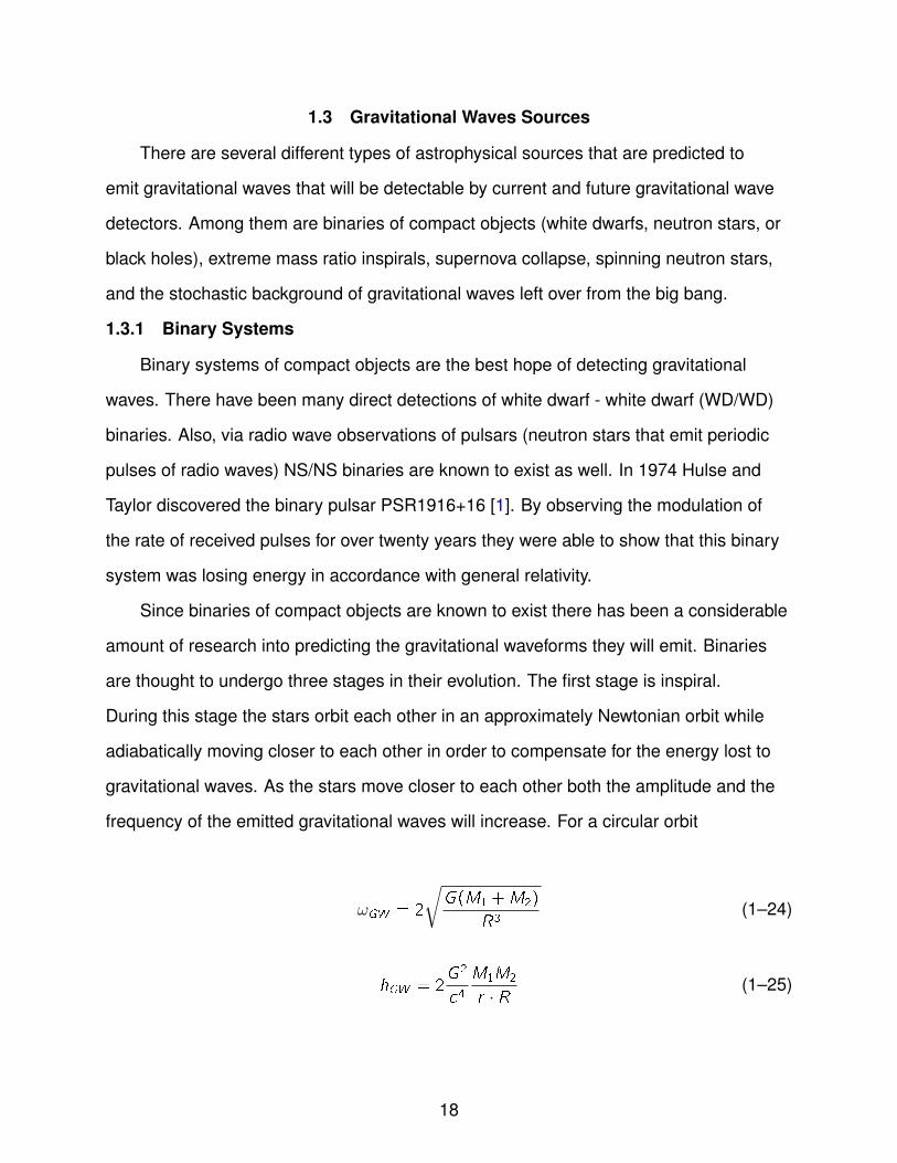
1.3.1 Binary Systems
Binary systems of compact objects are the best hope of detecting gravitational
waves. There have been many direct detections of white dwarf - white dwarf (WD/WD)
binaries. Also, via radio wave observations of pulsars (neutron stars that emit periodic
pulses of radio waves) NS/NS binaries are known to exist as well. In 1974 Hulse and
Taylor discovered the binary pulsar PSR1916+16 [1]. By observing the modulation of
the rate of received pulses for over twenty years they were able to show that this binary
system was losing energy in accordance with general relativity.
Since binaries of compact objects are known to exist there has been a considerable
amount of research into predicting the gravitational waveforms they will emit. Binaries
are thought to undergo three stages in their evolution. The first stage is inspiral.
During this stage the stars orbit each other in an approximately Newtonian orbit while
adiabatically moving closer to each other in order to compensate for the energy lost to
gravitational waves. As the stars move closer to each other both the amplitude and the
frequency of the emitted gravitational waves will increase. For a circular orbit
ωGW = 2
√G(M1 +M2)
R3(1–24)
hGW = 2G 2
c4M1M2
r · R(1–25)
18
Here R is the radius of the binary system and r is the distance from the binary to the
detector. By measuring the amplitude, the frequency, and the rate of change of the
frequency of the waves from a binary inspiral it is possible to determine its distance
from the earth. This information can be used to determine Hubble’s constant [2]. Using
post-Newtonian approximations the gravitational waveforms for the inspiral stage have
been computed out to order 7/2 [3].
The second stage is merger. During this stage the stars are no longer able to
maintain their orbits and they rapidly fall into each other. The result is a highly relativistic
collision. The gravitational waves from the merger stage must be computed numerically
[4]. The merger stage will be an invaluable test of general relativity in the strong field
limit. By monitoring the inspiral stage the initial conditions for a binary merger can be
determined and used in a numerical simulation. The results from the simulation can then
be compared to the measured waves from the actual merger.
The third stage is ringdown. During this stage the newly merged stars have formed
one object but have yet to settle down into an equilibrium state. During the ringdown
phase the emitted gravitational waves are exponentially damped oscillations. In the case
of a black hole binary system the two black holes will eventually settle down into a single
Kerr black hole, characterized only by its total mass and spin. The ringdown stage can
be modeled as linear perturbations to the Kerr spacetime.
In order to maximize a gravitational wave detector’s ability to detect binary
coalescences the signal processing method of matched filters is employed [5]. Matched
filters work by cross correlating the detector output with a pre-computed gravitational
waveform. Because the particular parameters of the binary coalescence are not known
ahead of time, an entire family of templates must be created with various values for the
masses, spins, and eccentricity of the orbit. In order to achieve an accurate template,
the waveforms from the inspiral, merger, and ringdown stages must be carefully put
together [6].
19

1.3.2 Extreme Mass Ratio Inspirals
Another source of gravitational waves are extreme mass ratio inspirals. Supermassive
black holes (104 to 107 solar masses) are thought to exist in the center of many galaxies.
When a smaller compact object orbits a supermassive black hole it loses energy to
gravitational radiation and inspirals into the supermassive black hole. One critical
difference between extreme mass ratio inspirals and roughly equal mass binaries
is that the small compact object spends much more time in the near vicinity of the
supermassive black hole, emitting 100,000’s or more cycles of gravitational waves.
These waves will contain detailed information about the strong field region surrounding
the black hole [7] and the value of the supermassive black hole’s multiple moments
[8]. This information will provide a test of the Kerr hypothesis, that all black holes are
uniquely determined by their mass and spin angular momentum. The gravitational
waves from extreme mass ratio inspirals are expected to be weak so the method of
matched filters must be used. To create templates for matched filters, the small compact
object is treated as a small perturbation to the supermassive black hole.
1.3.3 Supernova
The supernova of massive stars are an expected source of gravitational waves.
Gravitational waves are thought to be the strongest from type-II supernova, which is the
collapse of the core of a massive star to form a NS or BH. Most of the energy that is
lost in a supernova is carried away by neutrinos, but it is possible that enough energy
could be lost to gravitational waves to create a detectable signal. Gravitational waves
must come from the non symmetric portion of the collapse as spherical motions have
no quadrupole moment, and hence do not emit gravitational waves. The non spherical
portion of the supernova could be caused by the initial rotation of the star [9], low mode
convection [10], or anisotropic neutrino emission [11].
20

1.3.4 Rotating Neutron Stars
It is supposed that rapidly rotating stars could possibly emit detectable gravitational
waves via several mechanisms. When a neutron star is formed it is extremely hot,
rotating rapidly, and can be idealized as an axially symmetric perfect fluid. Perturbations
to this idealization result in a family of normal modes called the r-modes. The loss of
energy and angular momentum to gravitational radiation makes these modes unstable
[12] and the loss of energy and angular momentum will reduce the rotation rate of the
neutron star until it becomes stable. It is estimated that the rotation rate of a neutron star
may reduce to approximately 100 Hz one year after its formation [13]. The energy loss
to gravitational radiation should be sufficient to detect a newly formed spinning neutron
star in the Virgo Cluster [14].
An accreting neutron star could also be a source of gravitational waves. In a binary
system of a neutron star and a gas giant, the neutron star accretes mass from the gas
giant by tidal forces. This accretion increases the spin of the neutron star. One would
expect to find a wide variety of spin rates for accreting neutron stars, however, most
accreting neutron stars have spin rates close to 300 Hz. An explanation for this is that
asymmetries in the accretion could lead to gravitational waves that radiate away angular
momentum at the same rate as the accretion [15].
A rapidly rotating neutron star might not be perfectly symmetrical. Asymmetries, due
to either a strain in the star’s solid crust or due to the star’s magnetic field, could produce
detectable gravitational waves [16]. If a neutron star cools while undergoing oscillations
of the star’s fluid near the surface, it is possible that deformations could be ”frozen” into
the crust. If the interior of a neutron star is superconducting then the magnetic field will
be confined to the outer crust resulting in a much stronger magnetic field inside the crust
than outside the star. This strong magnetic field may be able to support large enough
deformations to produce gravitational waves.
21
1.3.5 Stochastic Background
In the same way the cosmic microwave background is electromagnetic radiation left
over from the beginnings of the universe, it is postulated that there may be an analogous
background of gravitational radiation. The cosmic microwave background only lets us
directly probe the universe back to the point when the universe first became transparent
to electromagnetic radiation, 380,000 years after the big bang. Since gravitational
waves interact very weakly with matter the detection of primordial gravitational waves
will allow us to directly probe the very early stages of the universe. One mechanism
for the creation of a stochastic background of gravitational waves left over from the
early universe is inflation. Since the measured anisotropies in the cosmic microwave
background agree so well with inflationary models of the universe it is expected that the
gravitational waves predicted by inflation should also be present [17].
1.4 Gravitational Wave Detectors
There are several different methods for detecting gravitational waves: resonant
mass detectors, pulsar timing, ground based laser interferometers, and space based
laser interferometers.
1.4.1 Resonant Mass Detectors
The first gravitational wave detector was a resonant mass detector built by John
Weber in the 1960s. A resonant mass detector is essentially a large metal cylinder that
will vibrate when a gravitational wave stretches it along its axis. A transducer is used
to convert the mechanical oscillations into an electrical signal which is then amplified
and measured. Since the amplifier adds noise to the signal the bars are constructed
as to have a narrow band resonance. This will allow a gravitational wave signal near
the resonance of the bar to build up to an amplitude large enough to overcome the
amplifier noise. Typical resonance frequencies are in the range 500-1500 Hz. In order to
overcome thermal noise fluctuations, modern resonant mass detectors are cryogenically
cooled to temperatures below 100 mK.
22

Even though the sensitivity of resonant mass detectors is so narrow in frequency,
it has been thought that they might be able to detect some kind of burst of gravitational
radiation. Such a burst could come from a supernova or the merger of two compact
objects. Detection should be possible if the burst wave carries enough energy in
the resonant mass detector’s sensitivity band. There have been several coincident
searches for burst events between resonant mass detectors [18] [19] and even between
resonant mass detectors and laser interferometers [20] [21]. While the search results
have all been negative so far they have placed upper limits on the rate of burst events.
Collaborations between resonant mass detectors have also been able to place an upper
limit on the gravitational-wave stochastic background [22].
1.4.2 Pulsar Timing
Millisecond pulsars emit radio waves at incredibly regular intervals. The pulsar
PSR J0437-4715 has been observed to have a root-mean-square error in the timing of
its pulses of 200 ns over a measurement time of ten years [23]. Pulsar timing is done
by comparing the time of arrival of the pulses with a prediction based on the various
parameters of the pulsar. The observed deviations from the prediction are called the
residuals. Pulsar timing can be used to search for gravitational waves by correlating the
residuals from the observations of several pulsars. While the effect of the gravitational
wave at each pulsar will be uncorrelated, the effect at the Earth will be.
Pulsar timing is most sensitive to gravitational waves in the very low frequency band
of 10−9 to 10−7 Hz. Sources at these frequencies include nearby supermassive massive
black hole binaries of 109 or more solar mass [24] and a stochastic background caused
by the large number of solar mass black hole binaries at redshifts of z = 2 [25].
1.4.3 Ground Based Laser Interferometers
Ground based laser interferometers are based on the simple design of a Michelson
interferometer. A coherent light source is split and sent down two perpendicular and
equal length arms, the light is reflected off of mirrors at the end of the arms, recombined
23

Figure 1-1. The lay out of a basic Michelson interferometer (left) and the lay out of anadvanced ground based gravitational wave interferometer (right) withFabry-Perot cavities, power recycling, and signal recycling mirrors. Notshown are mode cleaning optics after the laser and before thephotodetector.
at the beam splitter, and finally measured on a photodetector. A small difference in arm
lengths will result in a phase shift of the signal at the photodetector. In order to detect
a gravitational wave, the mirrors of the interferometer must be free to move along the
direction of the arms. From Equation 1–18 a gravitational wave will result in a length
change of
�lGW ≈ 1
2hL (1–26)
The largest ground based interferometers are built with 4 km arms and are expected
to observe gravitational waves of amplitude 10−19/√Hz . This corresponds to a change
in length measurement of 10−16meters/√Hz . In order to reach this sensitivity several
sources of noise must be accounted for. For example minute changes in the refractive
index of air or even the collision of air molecules with the interferometer optics would
dwarf the gravitational wave signals, so the entire interferometer is placed inside a
vacuum. Also the effective length of the interferometer can be increased by replacing the
mirrors of a Michelson interferometer with a Fabry-Perot cavity. The increase in effective
arm length is proportional to the finesse of the cavity. Ground based interferometers are
designed to operate at frequencies from approximately 10 Hz to 10 kHz.
24

Ground vibrations limit the performance of ground based interferometers at low
frequencies. The interferometer optics can be shielded from seismic noise by being
suspended by multiple pendulums. Since the pendulums are resonant at around 1 Hz,
higher frequency vibrations in the measurement band are suppressed.
Thermal noise within the interferometer optics will also be a limiting factor. Thermal
noise in the suspension system can cause the mirrors to move. The suspension system
is made out of a material with a high Q factor in order to confine the thermal noise to
a narrow frequency region. The optics themselves also fluctuate due to thermal noise.
The largest source of thermal noise is Brownian motion in the mirror coatings.
At high frequencies interferometers are limited by shot noise. Shot noise comes
from the quantization of light; random fluctuations in the arrival time of photons can
mimic a phase shift caused by a gravitational wave. Shot noise can be mitigated by
using more light. Increasing the number of photons averages out more of the random
fluctuations and increases the signal to noise ratio. By placing a mirror in front of the
beam splitter the outgoing light from the interferometer can be reflected back into the
arms. This technique is known as power recycling. Using this technique the light power
in the interferometer arms can reach hundreds of kilowatts. The intensity of the light
cannot be increased without limit, however, as increasing the intensity increases the
radiation pressure noise. Radiation pressure noise comes from uncorrelated quantum
fluctuations in the power in each arm of the interferometer. These small changes in the
power result in changes to the force applied to the mirrors by the light itself. This results
in spurious accelerations of the mirrors that act like gravitational waves. The radiation
pressure can be reduced by increasing the mass of the mirrors.
There are four large gravitational wave detector groups currently operating
worldwide, TAMA 300, GEO 600, VIRGO, and LIGO. TAMA 300, officially known as
the 300m Laser Interferometer Gravitational Wave Antenna, is a prototype detector
located in Japan. It has reached a sensitivity of 3 × 10⁻²¹/√Hz at 1.3 kHz [26] and
25

produced upper limits on the rate of gravitational wave bursts in a coincident search with
the LIGO detectors [27].
GEO 600 is a 600 m detector located in Germany. It is designed to incorporate
the latest advancements in seismic isolation and signal recycling. The latest seismic
isolation systems contain active control loops to sense and reduce the seismic noise.
Signal recycling is done by placing a mirror in front of the interferometer’s photodetector.
This forms a cavity through which the signal must pass. This resonance of this cavity
can be tuned to the frequency of an expected gravitational signal. This allows the
interferometer to operate in a narrow band mode with an improved performance in a
narrow but tunable frequency band.
VIRGO is a 3 km detector located in Italy. VIRGO is designed to have the best
performance of all ground based interferometers at low frequencies. It achieves this
performance by suspending all of the interferometer optics from a superattenuator. The
superattenuator is essentially a seven stage pendulum. However, in the superattenuator
the first five suspended masses are a large drum shaped mass known as a mechanical
filter. These mechanical filters help achieve excellent suppression of the vertical seismic
noise. Additionally, the top stage is connected to the ground by means of an inverted
pendulum with a resonant frequency of approximately 40 mHz [28]. The superattenuator
system allows the VIRGO interferometer to push the contribution of seismic noise down
to approximately 3 Hz.
LIGO is a network of two detectors, both in the United States, one in Washington
and the other in Louisiana. The site in Louisiana operates a 4 km interferometer while
the Washington site operates a 4km and a 2 km interferometer in parallel. LIGO is a
good complement to VIRGO in that is has better sensitivity at high frequencies while
VIRGO has better sensitivity at low frequencies. LIGO has produced several significant
astrophysical results including upper limits on the rate of low mass binary coalescences
[29], the rate of continuous gravitational wave signals (e.g. from rotating neutron stars)
26

[30], and the energy loss due to gravitational waves associated with gamma ray bursts
[31].
Both the VIRGO and LIGO detectors are currently being upgraded to their
Advanced VIRGO and Advanced LIGO configurations. These upgrades include a
large increase in laser power, monolithic suspensions made out of fused silica, heavier
mirrors, improved coatings, and signal recycling. The aim of these upgrades is to
achieve an improvement in sensitivity by a factor of ten. This increase in sensitivity
would lead to a 1000 times increase in the volume of space observed by the detectors.
It is predicted that together Advanced VIRGO and Advanced LIGO should be able to
observe approximately 40 gravitational wave events per year [32].
1.4.4 Space Based Laser Interferometers
Ground based interferometers are limited to observing gravitational waves above
10 Hz. However, there are many interesting sources of gravitational waves at lower
frequencies, such as binary coalescences of supermassive black holes, extreme mass
ratio inspirals, and the initial inspiral of white dwarf and neutron star binaries. By placing
a detector in space the low frequency seismic noise can be avoided entirely and much
longer arms can be used. While there are several options concerning the length of the
arms and the satellite configuration and orbits, the focus will be on the specific design
known as the Laser Interferometer Space Antenna (LISA). This is the subject of Chapter
2.
27
CHAPTER 2THE LASER INTERFEROMETRY SPACE ANTENNA (LISA)
The Laser Interferometer Space Antenna (LISA) is a joint mission between NASA
and ESA to observe gravitational radiation in the frequency range 10−4 to 1 Hz. Like
other detectors it will measure the fluctuations in the phase that laser light picks up
as it travels between free falling test masses. Unlike any other detector LISA will be
located in outer-space, enabling much greater separation between the test masses and
removing the seismic noise which limits ground based detectors at low frequencies.
LISA will consist of three spacecraft (SC) separated by 5 million km arranged in an
approximately equilateral triangle. Each SC will be in an independent heliocentric orbit
such that the LISA constellation will lag behind the Earth by 20 degrees and the plane
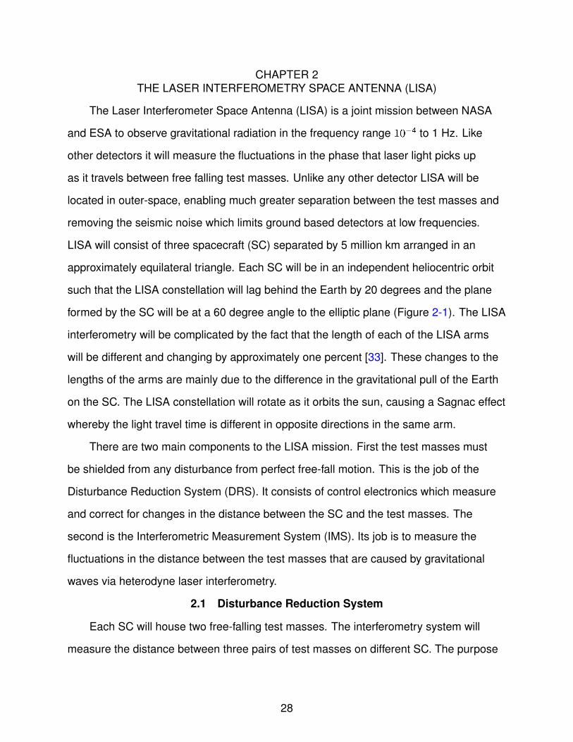
formed by the SC will be at a 60 degree angle to the elliptic plane (Figure 2-1). The LISA
interferometry will be complicated by the fact that the length of each of the LISA arms
will be different and changing by approximately one percent [33]. These changes to the
lengths of the arms are mainly due to the difference in the gravitational pull of the Earth
on the SC. The LISA constellation will rotate as it orbits the sun, causing a Sagnac effect
whereby the light travel time is different in opposite directions in the same arm.
There are two main components to the LISA mission. First the test masses must
be shielded from any disturbance from perfect free-fall motion. This is the job of the
Disturbance Reduction System (DRS). It consists of control electronics which measure
and correct for changes in the distance between the SC and the test masses. The
second is the Interferometric Measurement System (IMS). Its job is to measure the
fluctuations in the distance between the test masses that are caused by gravitational
waves via heterodyne laser interferometry.
2.1 Disturbance Reduction System
Each SC will house two free-falling test masses. The interferometry system will
measure the distance between three pairs of test masses on different SC. The purpose
28

Figure 2-1. The orbit of the three LISA SC. The center of the SC constellation will lagbehind the earth at an angle of 20 degrees. The plane formed by the threeSC is at a 60 degree angle with respect to the plane formed by the orbit ofthe Earth. The satellites are arranged in an approximately equilateraltriangle 5 million km apart from each other.
of the Disturbance Reduction System is to ensure that the test masses follow, as
close to possible, geodesic motion. Any spurious acceleration due to non gravitational
forces will mimic the effect of gravitational waves. These forces could come from solar
radiation, the interplanetary magnetic field, temperature variations on the SC, and
electrostatic and magnetic fields on the SC. While the SC will be specially designed to
minimize these forces on the test masses, these forces cannot be removed completely
so the test masses themselves will be designed to minimize the effect. The test masses
will be made out of a gold-platinum alloy specially designed to minimize their magnetic
susceptibility [34]. This has the added benefit of making the test masses heavy, reducing
any non-gravitational acceleration. Any excess electrostatic charge that builds up on the
test masses will be removed with UV-light via the photo-electric effect.
While the test masses will be shielded from non gravitational forces the SC will not.
In order to keep the SC from crashing into the test masses, the test mass positions will
be measured with capacitive sensors and micro-Newton thrusters will be used to correct
the SC’s position and orientation.
The Disturbance Reduction System will be tested on LISA Pathfinder which is
a precursor to the LISA mission scheduled to be launched in 2014. LISA Pathfinder
will house two test masses inside of one SC and will measure their motion with laser
29
interferometry. The masses will be shielded from any disturbances with a system very
similar to LISA’s. Pathfinder will allow the disturbance reduction system to be tested in
space before the main LISA mission.
2.2 Interferometric Measurement System
The Interferometric Measurement System is responsible for measuring the
fluctuations in the distance between the test masses that are caused by gravitational
waves. It is composed of optical components such as lasers, beam splitters, electro-optic
modulators (EOMs), photodetectors, and optical cavities. It is also composed of
electronic components such as MHz oscillators, frequency up-converters, analog
and digital control loops, and phasemeters. It will measure gravitational waves by
measuring the fluctuations in the phase accumulated by laser light as it travels between
freely falling test masses.
2.2.1 IMS Overview
Each SC will have two lasers which will send light to the other two SC (Figure
2-2). The laser light will be used to measure changes in the distance between the
test masses located inside the SC. The laser fields which travel counter clockwise
are denoted with an asterisk. Each arm is denoted with the number of the SC that
is opposite to that arm. Since the LISA constellation is rotating the travel time of the
light will be different in opposite directions along the same arm. So light travel times
in the counter clockwise direction are denoted with a prime. Each SC contains two
optical benches on which light is combined from the far SC, the local laser, and from the
opposite laser on the same SC. The entire optical bench will be fabricated form Zerodur
ceramic glass with each optical component attached using hydroxy catalysis bonding
[35]. Before the light is sent to the far SC it is expanded in a 40 cm diameter telescope.
2.2.2 Noise Requirement
The lasers will have a wavelength of 1064 nm. With an arm length of 5 million
km, a gravitational wave with strain 10−21 will create oscillations of amplitude 5 pm.
30

Figure 2-2. Diagram of the LISA satellites, IMS system, and the laser links between SC.Each SC contains two test masses, two optical benches, and two telescopesfor transmitting the outgoing laser beam. The received light is captured withthe same telescope. Not shown is the back link fiber which connectsadjacent optical benches on the same SC. Also shown is the namingconvention for the lasers and light travel times. Each laser shares a numberwith the SC it is located on. The lasers that transmit in the counter clockwisedirection are denoted with an asterisk. The travel times are named with thenumber of opposite SC with travel times in the counter clockwise directiondenoted with a prime.
31
This corresponds to 5 × 10⁻⁶ cycles of the laser light. LISA is limited by two noise
sources. The first is the shot noise of the lasers on the photodetectors. The light power
will be reduced to around 100 pW after traveling between spacecraft. This gives a
white noise of approximately 4 × 10⁻⁵ cycles√(Hz)
[36]. The second is the disturbances from
free fall in the motion of the test masses. The spurious test mass accelerations are
expected to be constant in frequency leading to a displacement noise that is inversely
proportional to frequency squared. At 2.8 mHz the displacement noise due to spurious
accelerations will become larger than the shot noise. The sum of the noise from all of
the subsystems which make up the IMS must perform better than the combination of
these two sources. So the requirement on any one subsystem of the IMS is taken to be
an order of magnitude lower. In this dissertation the following is taken to be the LISA
requirement for an individual system.
10−6
√1 +
(2.8mHz
f
)4cycles√Hz
(2–1)
2.2.3 Heterodyne Interferometry
Since the laser light will not be reflected back to the original SC, heterodyne
interferometry is used. We can model the electric field of the laser light with a complex
exponential
E1(t) = A1ei(2πν1t+ϕ1(t)) (2–2)
where A1 is the amplitude of the laser light, ν1 is the frequency, and ϕ1(t) is the time
varying phase of the laser light. The phase may contain terms due to the intrinsic laser
noise, the gravitational wave signals, photodetector noise, etc. Combining two such
laser fields on a photodetector yields
PD = |E1(t) + E2(t)|2 = A21 + A2
2 + 2A1A2cos (2πν12t + ϕ12(t)) (2–3)
32
where ν12 = ν1 − ν2 and ϕ12(t) = ϕ1(t) − ϕ2(t). LISA will measure the time varying
phase of the AC part of this signal. So we can write the photodetector signal as just the
phase
PD = ν12t + ϕ12(t) (2–4)
where the phase is in cycles. Heterodyning two lasers simply results in the difference of
their frequencies and phases.
2.2.4 LISA Sensor Signals
The incoming light is combined with the local laser on the science photodetector
(called PDSC see Figure 2-3). We can write the phase of laser 1 as
ν1t + ϕ1(t) (2–5)
and the phase of laser 2* from SC 2 as
ν2∗t + ϕ2∗(t − τ3′) + SC1(t) + h3′(t) (2–6)
where ν is the frequency of the lasers, ϕ(t) is the intrinsic phase noise of the lasers,
τ3′ is the time delay of the light traveling from SC 2 to SC 1 (along arm 3), SC1(t) is the
phase noise caused by the motion of the optical bench on SC 1 with respect to the test
mass, and h3′(t) is the phase change caused by gravitational waves while traveling from
SC 2 to SC 1. Combining the two laser fields on a single photodetector results in the
difference of their phases. The phase of the signal at PDSC is
PDSC = ν12∗t + ϕ1(t)− ϕ2∗(t − τ3′)− SC1(t)− h3′(t) (2–7)
This will form a signal in the range of 2-20 MHz. This signal contains the phase
fluctuations caused by the motion of the SC and the phase fluctuations accumulated
by the light as it travels between the SC due to gravitational waves. The light from the
adjacent optical bench is used to form two beat notes, one with the light directly from the
33

local laser and the other with the light from the local laser after it has been reflected off
of the test mass (PDA and PDTM).
PDA = ν11∗t + ϕ1(t)− ϕ1∗(t)− ϕ�ber(t) (2–8)
PDTM = ν11∗t + ϕ1(t)− ϕ1∗(t) + SC1(t)− ϕ�ber(t) (2–9)
Subtracting these signals removes the common laser and fiber noise between them
and leaves the phase fluctuations due to the motion between the SC and the test mass.
Finally, combining all three photodetector signals gives
PDSC + PDTM − PDA ≡ s21 = ν12∗t + ϕ1(t)− ϕ2∗(t − τ3′)− h3′(t) (2–10)
which only contains the differential laser noise and the gravitational wave signal. s21
is the signal formed on SC 1 with laser light sent from SC 2. There will be six of these
signals, one for each test mass. The extraction of the gravitational wave signals from the
laser noise is discussed in the next section.
2.2.5 Laser Noise Removal
If the laser phase noise was less than the requirement in Equation 2–1 then no
removal of the laser noise would be necessary. However, a typical free running laser is
fifteen orders of magnitude more noisy than the LISA noise limit. The removal of this
noise poses a serious technical challenge. The first step in the laser noise removal
is prestabilization. In the current configuration of LISA one laser is designated as the
master laser, which will be stabilized to a local reference on the SC. The other lasers
will be phase locked to the master. Several laser prestabilization methods have been
demonstrated including locking to an optical cavity [37] [38], a molecular resonance [39],
or an unequal arm heterodyne interferometer [40].
The next step in the laser phase noise removal is to stabilize the master laser using
the LISA arms as a reference. This technique is known as arm locking. Since the lasers
34

Figure 2-3. A simplified version of the layout of the LISA optical bench. There are twooptical benches on each SC. There is an optical fiber that transmits the lightto and from the adjacent bench. Photodetector SC measures a laser beatnote between the local laser and the received laser light from the far SC. Itcontains the signal due to the gravitational waves (picked up by the incominglight as it traveled from the far SC) and the signal due to the relative motionbetween the two SC. Photodetector TM is a beat note between the locallaser after it has been reflected off of the test mass and the laser from theadjacent bench. It contains the signal from the motion of the SC relative tothe test mass. Photodetector A is a beat note between the local laser andthe laser from the opposite bench. It is used to remove the laser noise fromthe measurement of the position of the SC relative to the test mass.
on the other SC are phase locked to the master laser, the light from the far SC can be
treated (to within the phase lock loop error) as being a mirror reflection of the master
laser delayed by the round trip travel time of the arms. The heterodyne signals between
the local and received laser light can be used to form an error signal in a control loop,
further stabilizing the master laser. Arm locking has been experimentally demonstrated
using a long cable length to simulate the lisa arms [41], as well as using electronic
delays [42] [43].
2.2.6 Time Delay Interferometry
The final step to remove the laser noise is a post processing technique known
as time delay interferometry (TDI). TDI removes the laser noise by forming linear
combinations of time delayed versions of the s data streams (Section 2.2.4). There are
35
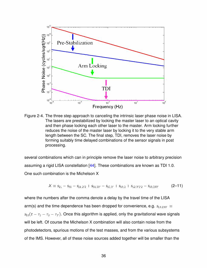
Figure 2-4. The three step approach to canceling the intrinsic laser phase noise in LISA.The lasers are prestabilized by locking the master laser to an optical cavityand then phase locking each other laser to the master. Arm locking furtherreduces the noise of the master laser by locking it to the very stable armlength between the SC. The final step, TDI, removes the laser noise byforming suitably time delayed combinations of the sensor signals in postprocessing.
several combinations which can in principle remove the laser noise to arbitrary precision
assuming a rigid LISA constellation [44]. These combinations are known as TDI 1.0.
One such combination is the Michelson X
X ≡ s21 − s31 − s21,2′2 + s31,33′ − s12,3′ + s13,2 + s12,3′2′2 − s13,233′ (2–11)
where the numbers after the comma denote a delay by the travel time of the LISA
arm(s) and the time dependence has been dropped for convenience, e.g. s13,233′ ≡
s13(t − τ2 − τ3 − τ3′). Once this algorithm is applied, only the gravitational wave signals
will be left. Of course the Michelson X combination will also contain noise from the
photodetectors, spurious motions of the test masses, and from the various subsystems
of the IMS. However, all of these noise sources added together will be smaller than the
36

requirement in 2–1. There are several factors which limit our ability to suppress the laser
noise with TDI algorithm to arbitrary precision. First we must know what delays to use
in order to apply the TDI algorithm. An small timing error in the delays will lead to an
imperfect cancelation of the laser noise. In the frequency domain this error will scale as
ϕ(t)− ϕ(t − �t) → ~ϕ(f )[1− e−i2πf �t
]≈ ~ϕ(f )(−i2πf �t) (2–12)
The requirement on the accuracy of the measured range is taken to be 1 meter (3 ns).
At a frequency of 1 mHz this corresponds to roughly 11 orders of magnitude noise
suppression. This is chosen so that TDI can be effectively applied in the case that either
pre-stabilization or arm-locking are used without the other.
Another limitation on the efficacy of TDI is the finite sampling rate at which the
LISA sensor signals are measured. The sensor signals will be sampled at a very low
rate (3-10 Hz). However, to apply the TDI algorithm the measured sensor signals must
be delayed in time with a precision of 3 ns. In order to shift the data stream with this
precision we must accurately interpolate between the data points which, at a 10 Hz rate,
are separated by 0.1 seconds. This can be done efficiently using fractional delay filters.
It has been found that only the surrounding 15 data points will be needed to interpolate
to the accuracy required by LISA when using a Lagrange interpolation [45].
In the actual LISA mission the arm lengths will be changing at a rate of up to 10
m/s and the rotation of the SC will cause a difference in the light travel time in opposite
directions along the same arm. TDI 2.0 takes these effects into account [46]. While
TDI 2.0 cannot be applied to arbitrary precision it will be sufficient to suppress the laser
noise below the LISA requirement.
2.2.7 Phasemeters
The phasemeter used in LISA is an IQ phasemeter with a tracking local oscillator
[42]. The beat note is mixed with a local oscillator forming an error signal that is used
in a control loop. This allows the local oscillator to match the phase noise of the beat
37

Figure 2-5. An IQ tracking phasemeter. Also shown is the Q output being filtered andsent to the delay lock loop for pseudo random noise (PRN) ranging.
note within the bandwidth of the control loop. The in band phase is added to the out of
band phase to form the phase measured by the phasemeter. This measurement must
be accurate to the order of the LISA requirement (Equation 2–1).
The phasemeter can accurately measure the phase, but it is driven by an imperfect
clock. The measurements made by the phasemeter are not perfectly periodic when
compared to a perfect clock. A timing error in the clock, �tclk , is converted into a phase
error in the measurement by �ϕ = �tclkν. The timing error of the clock is related to the
clock’s phase by �t = ��clkνclk . So the phase noise introduced by the clock noise is
given by
�ϕ = − ν
νclk�clk (2–13)
When the timing error is early the phase will be smaller than it should be resulting in
the minus sign.
2.3 Laser Communication System and Requirements
There are several tasks necessary for the success of LISA that require communications
between the SC. These are a transfer of the clock noise between SC, a measurement
of the range of the LISA arms, and a transfer of recorded data. These tasks could all be
38

done with traditional radio communications, but to reduce power consumption and the
mass of the SC they are done using the laser links between the SC.
2.3.1 Clock Noise Transfers
Each spacecraft will measure the phase of the beat notes and the phase lock loop
error relative to its own clock. In Section 2.2.4 the noise sources and gravitational waves
were written as compared to a perfect clock. In Section 2.2.7 it was shown that the clock
noise introduces phase noise in all the phasemeter measurements. With the clock noise
terms the sensor signals are
s21 = ν1∗2t + ϕ1∗(t)− ϕ2(t − τ3′)− h3′(t)−ν1∗2νclk
�1 (2–14)
s13 = ν13∗t + ϕ1(t − τ2′)− ϕ3∗(t) + h2′(t)−ν13∗νclk
�2 (2–15)
where �1 is the phase noise of the clock on SC 1 etc. The additional sensor signals
(s12 and s31) can be formed by cyclic permutation of the indicies. Inserting these into
Equation 2–11 produces
X = −ν12∗νclk
[�1 −�2,3′ +�1,2′2 −�2,3′2′2] +ν1∗3νclk
[�1 −�3,2 +�1,33′ −�3,233′] (2–16)
where the gravitational waves have been dropped for clarity. In order to cancel these
terms we must measure �1 − �2,3′ and �1 − �3,2. These terms are the difference
between the clock signals from the far SC delayed by the light travel time and the clock
signal of SC 1. To do so we modulate the clock signal onto the laser beams using an
electro optic modulator (EOM).
2.3.1.1 Electro-Optic Modulators
An EOM is an optical device used to modulate the amplitude or phase of laser light.
LISA will use phase modulators. In an EOM the laser light passes through a crystal that
exhibits a linear electro-optic effect (e.g. lithium niobate). This crystal is placed between
two electrodes. The electro-optic crystal experiences a change in its refractive index that
39

is proportional to the applied voltage to the electrodes. If a sinusoidal signal is applied to
the EOM the phase of the light is modulated as
e i [2πνt+ϕ(t)] → e i [2πνt+ϕ(t)+msin(2πFt+�(t))] (2–17)
where m is the amplitude of the modulation (in radians), F is the frequency of the signal,
and � is the time varying phase of the signal. This can be expanded in terms of Bessel
functions as
e i [2πνt+ϕ(t)+msin(2πFt+�(t))] = e i [2πνt+ϕ(t)]
∞∑n=−∞
Jn(m)e in[2πFt+�(t)] (2–18)
In the case that the amplitude of the modulation (m) is small the above expression
reduces to
J0(m)e i [2πνt+ϕ(t)] + J1(m)e i [2π(ν+F )t+ϕ(t)+�(t)] − J1(m)e i [2π(ν−F )t+ϕ(t)−�(t)] (2–19)
The result of the modulation is to create three distinct frequency components, a carrier
and an upper and lower sideband. The main carrier is at the original frequency of
the laser light and contains the original phase signal, but has been attenuated by the
factor J0(m). The two sidebands are separated in frequency from the main carrier by
the frequency of the modulation. The upper sideband contains the sum of the original
phase signal and the modulation phase signal, while the lower sideband contains their
difference. The sidebands are attenuated by J1(m). The modulation amplitude will be
chosen so that the sidebands contain 10 percent of the laser power [47].
2.3.1.2 Frequency Synthesizers
In order to suppress the clock noise terms to a level below the requirement
(Equation 2–1) the entire clock noise transfer chain must not add any phase noise
to the clock signals above the requirement. This includes the cables that transfer the
clock signal to the EOMs, the EOMs themselves, and the measurement of the phase
of the sidebands carrying the clock signals. Since the sideband signals contain less
40
power than the carrier they will have a lower signal to noise ratio than the main carrier
measurement. To overcome this noise, the phase of the clock signals will be amplified
by frequency up-conversion with a frequency synthesizer before they are modulated on
the EOMs. The result of a frequency up-convertersion is to multiply both the frequency
and phase of a signal by a factor α
sin [2πνt + ϕ(t)] → sin [2πανt + αϕ(t)] (2–20)
Each clock signal, �i will be up-converted by a factor of αi to a frequency in the
GHz range.
2.3.1.3 TDI with Clock Noise Removal
Figure 2-6 is a simplified version of the LISA mission. In this simplified version each
SC only has one laser and we don’t consider the laser links between SC 2 and SC 3.
The University of Florida Interferometry Simulator (UFLIS), which will be discussed in
Chapter 5, is based upon this simplified model of LISA. When the modulated light from
both the far and local lasers are combined on the photodetector they will form three
signals (Figure 2-7), the beat note between the lower sidebands (SSL), the beat note
between the carriers (CC ), and the beat note between the upper sidebands (SSU). All
other beat notes (e.g. between a lower sideband and the carrier) will be at frequencies
greater than the bandwidth of the photodetector. The upper and lower sideband signals
are given by
s21L = (ν12 + (α2 − α1) νclk) t + · · · − α1�1 + α2�2,3 −(ν12 + (α2 − α1) νclk)
νclk�1 (2–21)
s21U = (ν12 + (α1 − α2) νclk) t + · · ·+ α1�1 − α2�2,3 −(ν12 + (α1 − α2) νclk)
νclk�1 (2–22)
The phase noise of the carrier-carrier beat (s31) has been omitted for clarity. There are
similar equations for the s31 sidebands. We can combine the upper and lower sidebands
41

to obtain the clock noise.1
s∗21 ≡s21L − s21U
2α2
= �2,3 −�1 (2–23)
s∗31 ≡s31L − s31U
2α3
= �3,2 −�1 (2–24)
These signals are precisely what we need to measure to cancel the clock noise in
Equation 2–16. We can now modify the Michelson X combination to remove the clock
noise
X = s21 − s31 − s21,22 + s31,33 − s12,3 + s13,2 + s12,322 − s13,233
− ν21νclk
[s∗21 − s∗21,22
]+
ν31νclk
[s∗31 − s∗31,33
](2–25)
2.3.1.4 Clock Transfer Chain Noise Requirement
The combination s21L − s21U will contain shot noise at the photodetectors, and noise
from each part of the clock noise transfer chain such as the frequency synthesizers and
the EOMs. This noise will be multiplied by ν21νclk2α2
as in equations 2–23 and 2–25. The
noise multiplied by this factor must be lower than the LISA requirement. Thus the noise
requirement on the clock noise transfer chain is
νclk2α2
ν2110−6
√1 +
(2.8mHz
f
)4cycles√Hz
= 2× 10⁻⁴
√1 +
(2.8mHz
f
)4cycles√Hz
(2–26)
where we have used the current baseline design of upconverting to 2 GHz and assumed
the worst case scenario of a 20 MHz beat note.
42

Figure 2-6. The simplified model of LISA that UFLIS is based on. In this model each SConly has one laser and the laser link between SC 2 and 3 is not considered.There are also no test masses as the each SC is assumed to be stable tothe level of the gravitational waves. This way the s terms (Section 2.2.4) aresimply the photodetector output on each SC. Each laser passes through anEOM where it is modulated with both a PRN code and a frequencyup-converted version of the local clock.
2.3.2 Laser Ranging
In order to measure the distance between the spacecraft pseudo random noise
(PRN) codes are employed in a way similar to those used in GPS. A PRN code is a
series of ones and negative ones that has all the properties of a truly random process
1 The same result could be obtained by subtracting the carrier-carrier from one of thesideband-sideband beats. However, the term would be divided by α instead of 2α.
43

Figure 2-7. The laser modulation scheme. Each laser is modulated with a frequencyup-converted signal from the local clock producing sidebands at frequenciesαiνclk away from the carrier. The sidebands will be modulated with anamplitude designed to produce ten percent of the laser power in thesidebands. When combined with the light from the far SC three beat notesare formed, between the lower sidebands, the carriers, and the uppersidebands. The PRN code is also modulated onto the lasers causing aspread spectrum around the laser peaks. The PRN amplitude is chosen sothat one percent of the laser power is in the spread spectrum. This will be solow that the PRN spread spectrum will be buried under the shot noise level.
except that it is finite in length (Figure 2-8). A PRN code will be modulated onto the
phase of each laser with the same EOM used to modulate the clock signals. The code
will be recovered by the phasemeter on the far spacecraft. These sudden jumps in the
phase of the signal spread some of the power of the carrier into nearby frequencies
(Figure 2-7).
The codes used in LISA will be 1024 chips long and have a chip rate of approximately
1.5 MHz (Figure 2-8). The code period will then be about 0.6 ms or 1.8 × 10⁵ m. Such
a code will contain frequency components all the way down to the inverse of the code
period, which would be 1.5 kHz. Such frequency components are within the bandwidth
of the phasemeter and would be tracked and suppressed by the phasemeter. To remove
44

Figure 2-8. The PRN code and the Manchester encoding scheme. The chosen PRNcodes have 1024 chips that can be either positive or negative. The code isdesigned to mimic true noise in that is has very little correlation with itselfunless it is within one chip of itself. Since the PRN codes are produced andanalyzed digitally each chip has a finite number of samples. Each chip willhave 32 samples. The code is Manchester encoded by replacing everypositive chip with a rising edge and every negative chip with a falling edge.
these lower frequency components a Manchester encoding scheme is applied. Each +1
chip is replaced by a rising edge and each -1 chip is replaced by a falling edge (Figure
2-8). The Manchester encoding attenuates these lower frequency components.
In LISA, the laser light will be modulated with both the clock noise and the PRN
code before the optical bench. Each laser will be modulated with its own code. The
correlation will be done with the code from the far SC, but the code from the local SC
will also be present. The codes must be chosen such that there is no cross correlation
between the different codes so that the local code does not interfere with the generation
of the error signal. Six such codes were created by numerical optimization at the AEI
and were graciously loaned to us [48].
The PRN code is correlated with a locally generated version of the code. The
correlation is nearly zero unless the delay between the signals is within one chip length
45
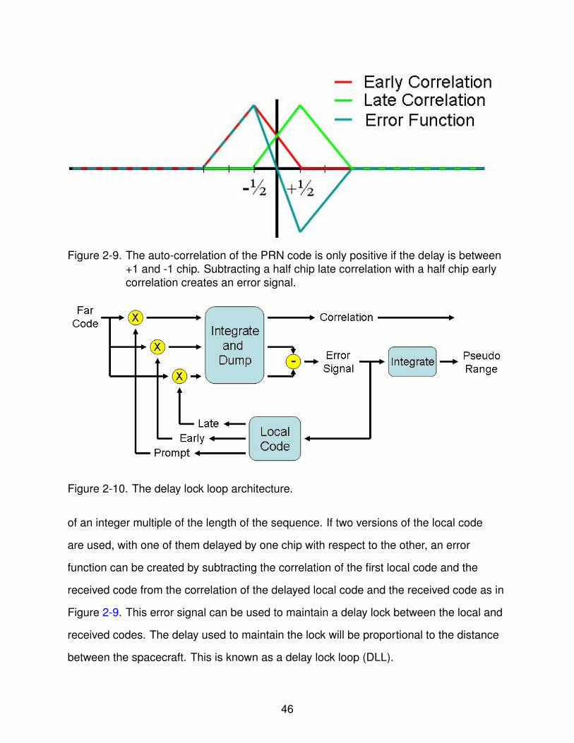
Figure 2-9. The auto-correlation of the PRN code is only positive if the delay is between+1 and -1 chip. Subtracting a half chip late correlation with a half chip earlycorrelation creates an error signal.
Figure 2-10. The delay lock loop architecture.
of an integer multiple of the length of the sequence. If two versions of the local code
are used, with one of them delayed by one chip with respect to the other, an error
function can be created by subtracting the correlation of the first local code and the
received code from the correlation of the delayed local code and the received code as in
Figure 2-9. This error signal can be used to maintain a delay lock between the local and
received codes. The delay used to maintain the lock will be proportional to the distance
between the spacecraft. This is known as a delay lock loop (DLL).
46
The architecture for the delay lock loop is shown in Figure 2-10. The error signal
is scaled and sent to the local code generator to advance or delay the local code. This
control signal is integrated to give the pseudo-range. This is the pseudo-range and not
the true range for two reasons. First the length of the LISA arms is much greater than
the correlation time. LISA will use the deep space network to determine the range to an
integer multiple of the correlation time/distance, then the pseudo range will be the left
over fraction of the correlation time. Second the start of the codes on different spacecraft
may not be synchronized. If the code at SC 1 starts at t1 and the code at SC 2 starts at
t2 then the pseudo ranges T1 and T2 will be
T1 =t2 + τ − t1 (2–27)
T2 =t1 + τ − t2 (2–28)
where τ is the fractional remainder of the delay time between the spacecraft. The
average of the pseudo ranges plus the rough estimate from the deep space network
gives the true range. The difference between the two pseudo ranges can be used to
determine the start time difference between the two codes. This will be important in
order to synchronize the sampling of data between SC.
When the code is sampled by the phasemeter it is digitized in its amplitude and
also in time. Thus the start of the code will be rounded to the next sample time. At
a sampling rate of 50 MHz, the sample time is 20 ns, leading to a measurement
limitation of 6 meters. A much better precision will be achieved due to the dithering
of the received PRN code by the noise present in the measurement. The shot noise
at the photodetector will cause the error signal to drive the local code away from the
incoming code. If the actual arrival of the incoming code is between samples of the local
signal processing, then the error caused by the shot noise will be biased toward the
closer sample time. The averaging of the range measurements over many correlations
47

will smooth out the random error caused by the shot noise and give a measurement
more precise than the sample time. While the length of the LISA arms will be changing
(up to 10 m/s) the change in the rate will be so slow that it can be taken as constant for
the purposes of measuring the range. Since the rate is constant a linear interpolation
will fit the data.
The amplitude of the PRN code is specified to be 0.14 rad/√Hz to make the power
in the spread spectrum one percent of the carrier’s power. At the high frequencies of the
PRN code the laser noise will be dominated by shot noise at the photo detectors. In fact
the shot noise will completely bury the PRN code as in Figure 2-7.
Another way to measure the arm lengths is to simply apply the TDI combinations in
post processing for a variety of delays until the laser noise in the LISA band has been
minimized [49]. The concern is that by minimizing the signal in the LISA band one might
minimize the gravitational wave signals instead of the laser noise. Another scheme is to
apply a modulation tone to each laser just outside of the measurement band, at say 1.1
Hz. The minimization could be applied to just this frequency band instead of the entire
laser noise in the LISA band.
48

CHAPTER 3THE UNIVERSITY OF FLORIDA LISA INTERFEROMETRY SIMULATOR
The University of Florida LISA Interferometry Simulator (UFLIS) is a hardware
simulator of the LISA Interferometric Measurement System (IMS). The purpose of UFLIS
is to provide an apparatus that can be used to test various aspects of LISA technology.
UFLIS is unique in that it has the capability to reproduce realistic light travel time delays
using an electronic phase delay (EPD). The EPD also allows for the simulation of
Doppler shifts in the frequency of the laser light. UFLIS has been used to test TDI [37]
[50], arm locking [43] [51], and TDI with time changing delays [52].
3.1 UFLIS Concept
The basic concept of UFLIS is to model as closely as possible the simplified
LISA interferometry in Figure 2-6. In this simplified version of LISA each SC only
has one laser, there are no test masses, and the laser links between SC 2 and 3 are
not considered. The laser on SC 1 is the master laser and is stabilized to an optical
reference while the lasers on the other two SC are phase locked to the master. In UFLIS
the long (16 s) delay time between the SC are simulated by measuring the phase of the
laser light, storing it in memory, and electronically regenerating it. In order to measure
the phase of the laser light, each of the three lasers in UFLIS (representing each SC) is
heterodyned with a fourth laser known as the reference laser (Figure 3-1). In this way
the frequency of the laser light is brought down to the MHz range allowing the phase
to be measured, stored, and regenerated. Since each laser is heterodyned with the
reference laser before it is delayed or combined with any other laser, the only effect of
the reference laser is to replace the phase noise of each laser with
ϕ1(t) → ϕ1R(t) ≡ ϕ1(t)− ϕR(t) (3–1)
Since the reference laser is independent of each other laser it only increases the
laser noise by a factor of√2.
49

Figure 3-1. How the EPD unit models the long travel times of the LISA arms. Thereference laser is used to form a beat note with both Laser 1 and 2. TheLaser 1 beat note is recorded, stored in memory, and regenerated. Thedelayed signal is then combined with the Laser 2 beat note with an electronicmixer.
3.2 Laser Bench Top Set-Up
The original layout of the laser bench top of UFLIS is shown in Figure 3-2 and
is described in [37]. In the original layout the lasers were combined in free space. In
the current layout all four lasers are coupled into polarization maintaining fibers via
fiber couplers from Schafter+Kirchhoff (model 60SMS-1-4-A11-03). Each laser is sent
through a fiber-optic EOM from Jenoptik (model PM1060HF) in order to upgrade UFLIS
to include clock noise transfers and PRN ranging (Figure 3-2). In both layouts the
reference laser and laser 1 are both stabilized to reference cavities housed in a vacuum
tank. In the previous layout mode matching lenses were used to match the mode of
each of the numbered lasers to the reference laser before they were measured at the
photodetectors. In the current layout polarization maintaining fiber splitter/combiners
from Opto-Link Corporation are used to split the reference laser three ways and combine
50

Figure 3-2. The previous set up of the laser bench top for UFLIS. Not shown are theFaraday isolators after each laser, the mode matching lenses, theelectro-optic modulator, quarter wave plate, and other optics associated withthe Pound-Drever-Hall locking scheme.
Figure 3-3. The current set up of the laser bench top for UFLIS. Not shown are theFaraday isolators after each laser, the mode matching lenses and mirrorsused to couple the laser light into the fibers, the electro-optic modulator,quarter wave plate, and other optics associated with the Pound-Drever-Halllocking scheme. The fibers used to form the beat notes and thephotodetectors are shown in Figure 3-4.
it with lasers 1, 2, and 3 (Figure 3-4). The fiber components are connected using
mating sleves from Thorlabs (model ADAFC2-PMW). The combined laser fibers are
coupled directly to photodetectors from Electro-Optic Technology Incorporated (model
ET-300A-FC-DC).
51

Figure 3-4. The formation of optical beat notes in the current UFLIS set up. A three wayfiber splitter is used to split the reference laser, while three two way fibercombiners are used to form beat notes between each of the numberedlasers and the reference laser. The fibers containing the beat notes aredirectly attached to the photodetectors.
3.3 Prestabilization
Both the reference laser and Laser 1 are frequency stabilized to Zerodur optical
cavities housed in a vacuum tank. The lasers are locked to the optical cavities by the
Pound-Drever-Hall method [53]. This prestabilization set-up was designed to emulate
as realistically as possible the baseline design for LISA. The UFLIS prestabilization was
shown to meet the original frequency stabilization requirement of 30Hz/√Hz [54] [37].
3.4 Electrical Components
The photodetector signals of the beat notes between the numbered lasers and the
reference laser are used to simulate the individual laser signals in LISA (Figure 3-5). In
LISA each laser signal is split, with ¡ 0.1 percent used to form the local beat note and the
other part sent to the opposite SC. In UFLIS each simulated laser signal is electronically
split, with one half sent to the EPD unit (simulating the light travel time between SC) and
the other half being electronically mixed (Mini Circuits ZAD-6+) with the electronically
delayed simulated laser signal from the other SC. The electronic mixers (and low pass
filters) simulate the photo detectors in LISA on which the local laser and far laser are
beat together. The outputs of the mixers simulate the sij signals (Equation 2–10) and are
sent to a phasemeter to be measured.
52
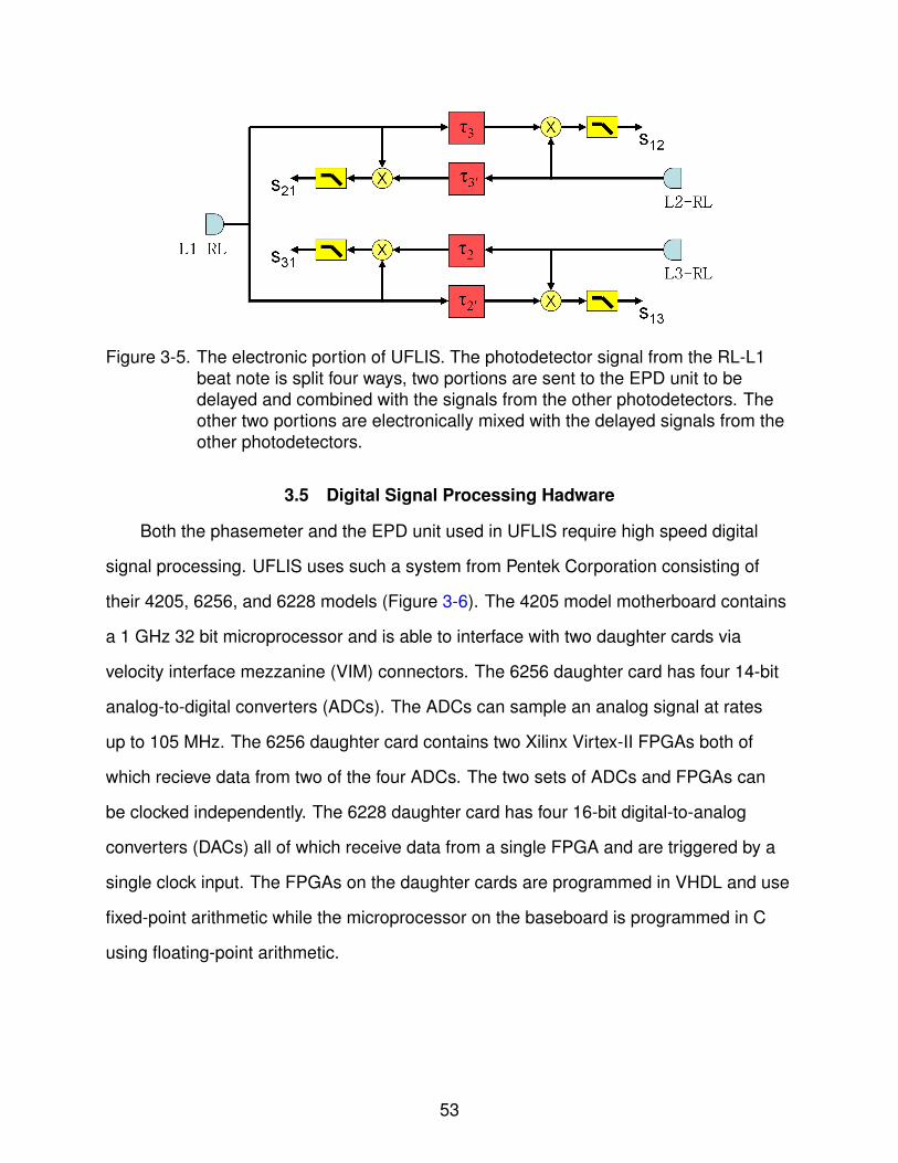
Figure 3-5. The electronic portion of UFLIS. The photodetector signal from the RL-L1beat note is split four ways, two portions are sent to the EPD unit to bedelayed and combined with the signals from the other photodetectors. Theother two portions are electronically mixed with the delayed signals from theother photodetectors.
3.5 Digital Signal Processing Hadware
Both the phasemeter and the EPD unit used in UFLIS require high speed digital
signal processing. UFLIS uses such a system from Pentek Corporation consisting of
their 4205, 6256, and 6228 models (Figure 3-6). The 4205 model motherboard contains
a 1 GHz 32 bit microprocessor and is able to interface with two daughter cards via
velocity interface mezzanine (VIM) connectors. The 6256 daughter card has four 14-bit
analog-to-digital converters (ADCs). The ADCs can sample an analog signal at rates
up to 105 MHz. The 6256 daughter card contains two Xilinx Virtex-II FPGAs both of
which recieve data from two of the four ADCs. The two sets of ADCs and FPGAs can
be clocked independently. The 6228 daughter card has four 16-bit digital-to-analog
converters (DACs) all of which receive data from a single FPGA and are triggered by a
single clock input. The FPGAs on the daughter cards are programmed in VHDL and use
fixed-point arithmetic while the microprocessor on the baseboard is programmed in C
using floating-point arithmetic.
53

Figure 3-6. The digital signal processing system. The 6256 daughter card handles theinput of the phasemeter and EPD unit. The 4205 motherboard handles thetransfer of data from the input daughter card to the 6228 output daughtercard and to the PC.
3.6 Phasemeter
The phasemeter used in UFLIS is an IQ tracking phasemeter as described in
Section 2.2.7. The phasemeter is programmed on the FPGAs of the 6256 daughter
card. In this thesis all measurements are made with the phasemeter clocked with a 50
MHz external source. Within the tracking loop the signal is down sampled by a factor of
27 with a six stage CIC filter. The data output to the baseboard is not the phase but the
in-band frequency which is further down sampled by a factor of 215 with a six stage CIC
filter. This gives a data rate of 11.92 Hz. The phase is reconstructed by integrating the
frequency data in post-processing. In the LISA measurement band (0.1 mHz to 1 Hz)
the UFLIS phasemeter is limited by timing jitter and temperature dependent phase noise
[52] and can be modeled as having a 1/√f dependence.
The UFLIS phasemeter noise is measured by electronically splitting a MHz signal
and measuring the phase with two separate phasemeters on the same 6256 daughter
54

Figure 3-7. Linear spectral density of the results of two measurements to of the UFLISphasemeter system. A VCO signal was split and measured with thephasemeter on two separate channels of the DSP system. The red curve isthe initial VCO signal, the magenta curve is the difference in the twomeasurements when made on the same FPGA, the blue curve is thedifference in the two measurements when made on separate FPGAs afterfractional delay filtering, and the cyan curve is the difference in the twomeasurements before fractional delay filtering.
card. The noise added by the digital signal processing hardware is found by taking the
difference of the two measurements. If the measurement is made between channels 1
and 2 or 3 and 4 (i.e. on the same FPGA) the measurements can be subtracted with
no post processing. However, if two measurements are made on separate FPGAs (e.g.
channels 1 and 3) then there will be a small delay between the two measurements. This
delay is much smaller than the 11 Hz sampling rate and therefore requires fractional
delay filtering. The results of such a measurement with a 12 MHz signal from a VCO are
plotted in Figure 3-7.
55

3.7 Electronic Phase Delay Unit
The EPD unit utilizes the entire digital signal processing system outlined in Section
3.5. There are two configurations of the EPD unit, the sample and hold EPD unit and the
phasemeter EPD unit.
In the sample and hold EPD unit a signal is sampled by the ADCs on the 6256
daughter card at a rate of 100 MHz. The sampled signal is down sampled by a factor of
8 to 12.5 MHz before it is sent to the 4205 baseboard. On the baseboard it is stored in
memory for up to 2.5s. After the signal has been delayed it is sent to the 6228 daughter
card where is is converted back to analog. The disadvantage of the sample-and-hold
method is that the high data rate limits the time that the data can be stored in memory
to 2.5s. On the baseboard the data is stored in buffers 1024 data points long. This limits
the precision of the delay unit to 82µs . Figure 3-8 shows the results of a test of the
sample and hold EPD unit. The sample and hold delay performs slightly worse than the
phasemeter.
The phasemeter EPD unit overcomes the limited delay time of the sample and
hold method by measuring the frequency of the sampled signal with a phasemeter
programmed on the input daughter card. The measured frequency is down sampled to
99.66 kHz and sent to the baseboard where it can be stored in memory for hundreds
of seconds. It is stored in buffers 1024 data points long, limiting the precision to 10
ms. The frequency data from the baseboard is sent to the 6228 daughter card where
it is added to an offset and integrated and used as the phase input of a numerically
controlled oscillator (NCO). The offset can be programmed to be any frequency allowing
the phasemeter EPD unit to simulate Doppler shifts in the frequency of the laser signals
while preserving the frequency fluctuations of the signals at low frequencies.
3.8 Previous Experiments with UFLIS
There have been several experiments using UFLIS to test LISA interferometry.
The first used the sample and hold version of the delay unit and a precursor to the
56

Figure 3-8. Linear spectral density of the results of a test of the performance of thesample and hold EPD unit. A 2 MHz signal from a function generator wassplit with one half sent directly to the phasemeter and the other half sentthrough the sample and hold delay and then to the phasemeter. The initialsignal is plotted in red and the difference between the two measurements isplotted in magenta.
current phasemeter-running at much slower speeds-to test TDI in the case of static arms
and with two second delays. This experiment showed that TDI was able to suppress
the laser noise, but the experiment was limited by the noise of the oscillator used to
heterodyne down the laser beat signals [55].
Another experiment used the phasemeter version of the EPD unit and the current
phasemeter to test TDI in the case of static arms and the full 16 second delays. It was
found TDI was able to suppress the laser noise to the limit of the EPD unit, which is
about an order of magnitude greater than the LISA requirement [50].
UFLIS has also been used to test arm locking. The first experiment tested single
arm locking using kHz electronic oscillators and a precursor to the current EPD unit with
a half second delay [56]. The next experiment used prestabilized lasers and the current
57

EPD unit with a 1 second delay and Doppler shifts to produce a realistic test of single
arm locking [57]. UFLIS also played a key role in the discovery of ”frequency pulling” an
issue that comes about due to errors in the estimation of the Doppler shifts [58]. The
latest experiments in arm locking have validated the performance of dual and modified
dual arm locking [51].
The EPD unit has been upgraded to produce time changing time delays as well as
inject simulated gravitational wave signals into the measurement. This upgraded version
of the EPD unit was used to experimentally test TDI 2.0 [59].
3.9 Goals of this Work
The goal of the work contained in this thesis is to test the individual components of
the laser communication systems using the hardware of UFLIS. This includes testing
the phase fidelity of frequency up converters and EOMs, testing the clock noise transfer
concept, and designing and implementing a DLL in hardware. It is also the goal of this
work to integrate the laser communication systems into UFLIS to construct a more
complete and realistic LISA simulator.
58

CHAPTER 4VERIFICATION OF INTER SPACE CRAFT CLOCK TRANSFER
4.1 Tests of Frequency Synthesizers
As part of the clock transfer chain the frequency synthesizers must be able to
convert the frequency of the LISA clocks from 50 MHz to 2 GHz while adding less phase
noise than the requirement in Equation 2–26. Three different systems for frequency
up-converting a 50 MHz signal to 2 GHz were tested. One method was to use the built
in phase-lock loop (PLL) on a Stanford Research Systems CG635 clock generator. The
second method used a 2 GHz voltage-controlled oscillator (VCO) with a custom built
PLL. The third method was a custom built frequency synthesizer by Rupptronik capable
of converting a 50 MHz signal to a signal between 1.980 and 2.020 GHz in steps of 100
kHz.
Figure 4-1 is a diagram of the experimental set up to test the various frequency
up-conversion systems. A common MHz oscillator is frequency up-converted by
two independent systems to the same GHz frequency (at or near 2 GHz). Both
up-converted signals are mixed with a common GHz oscillator using a Mini-Circuits
ZX05-C24-S+ mixer (all GHz signals are mixed with this mixer and split with a
Mini-Circuits ZFSC-2-2500-S+ in this thesis). The frequency of this oscillator is set
to produce a 1 MHz difference signal after low pass filtering (Mini-Circuits VLFX-80).
These 1 MHz signals are measured with the UFLIS phasemeter (Section 3.6) and the
difference between the two measured phases is calculated in post-processing. The
difference in phase is attributed to the differential noise added between the frequency
up-conversion systems.
4.1.1 Stanford Clocks
The Stanford Research Systems CG635 clock generator is capable of producing
clock outputs up to 2 GHz. It has a built in PLL that can lock the phase of the clock
output to the phase of a 10 MHz signal. Two clock generators are locked to a common
59

Figure 4-1. Set up of the experiment to measure the noise added to the clock transfer bythe frequency up-conversion process. Three different frequencyup-conversion systems were tested in this configuration. A common MHzsignal is frequency up-converted to a signal around 2GHz by twoindependent frequency up-conversion systems. The resulting GHz signalsare mixed down to 1 MHz with a common GHz oscillator. The two 1 MHzsignals are measured by the UFLIS phasemeter. The difference in themeasured phases can be attributed to the differential noise between the twoup-conversion systems.
10 MHz signal and each output a 2 GHz signal which is mixed with a 1.999 GHz
oscillator. The phase of the resulting 1 MHz signals were measured by the UFLIs
phasemeter. In post processing these phases are subtracted resulting in the difference
in the phase noise added by each Stanford clock generator. The results are plotted in
Figure 4-4 along with the results of the other methods. The Stanford clock generators
are worse than the requirement by about a factor of 25 at 3 mHz.
4.1.2 Custom Phase Lock Loop
The second frequency up-conversion method that was tested used a 2 GHz VCO
(Mini-Circuits ZX95-2015-S+) and a custom built PLL. The VCO has a 0-5 volt tuning
port to adjust the frequency of the oscillator from 1.975 to 2.015 GHz. Figure 4-2 is
a diagram of the custom PLL built for the 2 GHz VCO. The feedback loop starts with
a Centellax UXN14M9PE frequency down converter that converts the 2 GHz output
of the VCO to a 10 MHz signal. Figure 4-3 is a diagram and results of differential test
of the noise added by two of these down converters. A common 2 GHz signal was
down-converted to 4 MHz by two down converters. Both signals were measured by the
60

Figure 4-2. The PLL used to lock the 2 GHz VCO to a 10 MHz signal. The 2 GHz outputis down converted to a 10 MHz signal which is sampled by the AcromagDSP board along with the original 10 MHz signal. Both signals are multipliedand filtered. The output of the filter is scaled with a proportional and integralpass before being output to the 5 Volt tunning port of the VCO.
phasemeter and subtracted in post processing. The measurement was limited by the
noise of the phasemeter.
Both the down converted signal and the 10 MHz signal that the VCO is locked to
are sampled by an Acromag PMC-AX3065 digital signal processing board at a rate of
64 MHz. The two signals are digitally multiplied and filtered. This output is scaled by a
proportional and integral pass added to an offset and output to the 5 Volt tuning port of
the VCO.
Just like the experiment with the clock generators, the custom frequency up-conversion
systems are locked to a common 10 MHz oscillator, output a 2 GHz signal, and are
mixed down to 1 MHz with a common 1.999 GHz signal. The results are plotted in
Figure 4-4 along with the results of the other methods. The custom up-converters are
worse than the requirement by about a factor of 250 at 3 mHz.
4.1.3 Rupptronik Frequency Synthesizers
The final up-conversion method that was tested was a custom built frequency
synthesizer by Rupptronik capable of converting a 50 MHz signal to a signal between
1.980 and 2.020 GHz in steps of 100 kHz. In this experiment two Rupptronik synthesizers
61

Figure 4-3. Set up and linear spectral density of the results of a differential test of thefrequency down converters. The measurement was limited by theperformance of the phasemeter.
up-convert a common 50 MHz signal to 2.001 GHz, and these signals are mixed down
to 1 MHz with a common 2.000 GHz oscillator. The results of the measured differential
phase noise between the two frequency synthesizers are plotted in Figure 4-4 along
with the results of the other methods. The Rupptronik frequency synthesizers meet the
requirement for all frequencies.
4.1.4 Results
Of the three methods for frequency up-conversion, only the frequency synthesizers
from Rupptronik met the requirement over the entire frequency band (Figure 4-4.
The differential measurement suffers from two drawbacks, one that there may be
some common noise between the two synthesizers that is canceled in the differential
measurement, and two that the synthesizers were both operated at the same frequency
up-conversion factor. In LISA the up-conversion factor must be different in order
to produce sideband-sideband beat notes at frequencies separate from the main
62

Figure 4-4. Linear spectral density of the three different differential tests of the frequencyup-conversion process. Only the frequency synthesizers from Rupptronikmeet the requirements.
carrier-carrier beat note. Another experiment (Section 4.4) tested two of these
synthesizers while up-converting to different frequencies.
4.2 Tests of Electro-Optic Modulators
The EOMs used to modulate the clock signal onto the laser beams may introduce
some noise themselves. Changes in temperature will cause changes in the length and
refractive index of the electro-optic crystal, resulting in an unwanted modulation of the
laser light. Two experiments were carried out to measure the phase noise added to the
clock noise transfer by the EOMs. The first was an initial test perfomed at a modulation
frequency of 5 MHz. The second tested the EOM at a modulation frequency of 2 GHz.
The EOM that was tested was the integrated optical phase modulator from Jenoptik,
model PM1060HF. The input and output of this phase modulator is coupled to a
polarisation maintaning optical fiber. Four of these phase modulators are used in
the UFLIS optical benchtop (Section 3.2). The following experiments on the EOMs utilize
the optical set up of UFLIS.
63

4.2.1 MHz Test
Figure 4-5 is a diagram of the experiment to determine the noise added to the clock
noise transfer by the EOM when it is modulated at 5 MHz. The experiment used the
optical set-up of UFLIS as described in Section 3.2. A 5 MHz signal is modulated onto
Laser 2 which is offset phase locked to the reference laser at 10 MHz. Three signals are
measured at the photodetector; the lower sideband at 5 MHz, the carrier at 10 MHz, and
the upper sideband at 15 MHz. The phases of these signals are measured to be
SL =(ν2R − F )t + ϕ(t)−�(t)− (ν2R − F )
Fclk�clk (4–1)
C =ν2Rt + ϕ(t)− ν2RFclk
�clk (4–2)
SU =(ν2R + F )t + ϕ(t) + �(t)− (ν2R + F )
Fclk�clk (4–3)
where ν2R is the beat note frequency, ϕ(t) is the beat note phase, F is the frequency
of the modulation signal, �(t) is the modulation phase, Fclk is the frequency of the
phasemeter clock, and �clk is the phase of the phasemeter clock.
The signal from the photodetector is sent to channel 1 of the 6256 daughter card
(Section 3.5) where it is digitally split so that three separate phasemeters on the same
FPGA can each measure one of the three signals. The modulation signal is directly
measured on channel 2.
M = Ft +�(t)− F
Fclk�(t) (4–4)
The noise added to the clock noise transfer can be found by forming
(SU − SL)/2−M (4–5)
in post processing. The results of a two hour measurement are plotted in Figure 4-6.
The EOM meets the requirement at all frequencies.
64

Figure 4-5. The experimental set up for the test of the EOM’s phase stability at 5 MHz.The experiment uses the optical set up of UFLIS. Laser 2 is phase locked tothe reference laser at an offset frequency of 10 MHz. Laser 2 is alsomodulated with a 5 MHz signal creating sidebands at 5 MHz and 15 MHz.The upper and lower sidebands are measured at channel 1 of thephasemeter while the modulation signal is directly measured on channel 2.
4.2.2 GHz Test
Figure 4-7 is a diagram of the experiment to determine the phase fidelity of the
EOM when modulated at 2 GHz. The experiment used the optical set-up of UFLIS as
described in Section 3.2. Laser 2 is modulated with a 2 GHz signal while a 1.999 GHz
signal is used to offset phase-lock Laser 2 to the reference laser. The three signals
that result from the hetrodyning of Laser 2 and the refrence laser are: a 1 MHz lower
sideband which has been aliased from negative 1 MHz, the 1.999 GHz carrier, and the
3.999 GHz upper sideband which is outside the bandwidth of the photodetector. The
phase noise of the lower sideband and the carrier can be written as
SL =(−ν2R + F )t − ϕ(t) + �(t) (4–6)
C =ν2Rt + ϕ(t) (4–7)
The aliasing from negative frequencies results in the inversion of the phase of the lower
sideband. The signal from the photodetector is split with one half (the lower sideband)
low passed filtered and sent to the phasemeter, and the other half (the carrier) is mixed
65
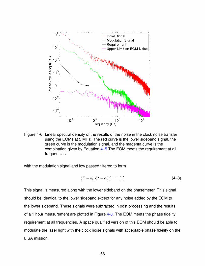
Figure 4-6. Linear spectral density of the results of the noise in the clock noise transferusing the EOMs at 5 MHz. The red curve is the lower sideband signal, thegreen curve is the modulation signal, and the magenta curve is thecombination given by Equation 4–5.The EOM meets the requirement at allfrequencies.
with the modulation signal and low passed filtered to form
(F − ν2R)t − ϕ(t) + �(t) (4–8)
This signal is measured along with the lower sideband on the phasemeter. This signal
should be identical to the lower sideband except for any noise added by the EOM to
the lower sideband. These signals were subtracted in post processing and the results
of a 1 hour measurement are plotted in Figure 4-8. The EOM meets the phase fidelity
requirement at all frequencies. A space qualified version of this EOM should be able to
modulate the laser light with the clock noise signals with acceptable phase fidelity on the
LISA mission.
66

Figure 4-7. The experimental set up for the test of the EOM’s phase stability at 2 GHz.The experiment uses the optical set up of UFLIS. An offset frequency of1.999 GHz is used to phase lock Laser 2 to the reference laser. Amodulation signal at 2.000 GHz is applied to Laser 2 creating a lowersideband at 1 MHz. The modulation signal is electronically mixed with thecarrier signal. The resulting signal is low passed filtered resulting in a 1 MHzsignal which is measured at channel 1 of the phasemeter. The lowersideband is also filtered and measured at channel 2 of the phasemeter.
Figure 4-8. Linear spectral density of the results of the noise in the clock noise transferusing the EOMs at 2 GHz. The red curve is the initial lower sideband signaland the magenta curve is the difference between the lower sideband and thecarrier mixed with the modulation signal. The EOM meets the requirement atall frequencies.
67
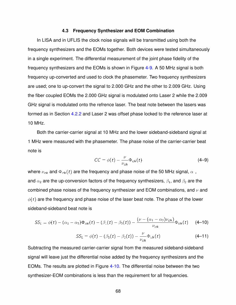
4.3 Frequency Synthesizer and EOM Combination
In LISA and in UFLIS the clock noise signals will be transmitted using both the
frequency synthesizers and the EOMs together. Both devices were tested simultaneously
in a single experiment. The differential measurement of the joint phase fidelity of the
frequency synthesizers and the EOMs is shown in Figure 4-9. A 50 MHz signal is both
frequency up-converted and used to clock the phasemeter. Two frequency synthesizers
are used; one to up-convert the signal to 2.000 GHz and the other to 2.009 GHz. Using
the fiber coupled EOMs the 2.000 GHz signal is modulated onto Laser 2 while the 2.009
GHz signal is modulated onto the refrence laser. The beat note between the lasers was
formed as in Section 4.2.2 and Laser 2 was offset phase locked to the reference laser at
10 MHz.
Both the carrier-carrier signal at 10 MHz and the lower sideband-sideband signal at
1 MHz were measured with the phasemeter. The phase noise of the carrier-carrier beat
note is
CC = ϕ(t)− ν
νclk�clk(t) (4–9)
where νclk and �clk(t) are the frequency and phase noise of the 50 MHz signal, α1,
and α2 are the up-conversion factors of the frequency synthesizers, β1, and β2 are the
combined phase noises of the frequency synthesizer and EOM combinations, and ν and
ϕ(t) are the frequency and phase noise of the laser beat note. The phase of the lower
sideband-sideband beat note is
SSL = ϕ(t)− (α1 − α2)�clk(t)− (β1(t)− β2(t))−(ν − (α1 − α2)νclk)
νclk�clk(t) (4–10)
SSL = ϕ(t)− (β1(t)− β2(t))−ν
νclk�clk(t) (4–11)
Subtracting the measured carrier-carrier signal from the measured sideband-sideband
signal will leave just the differential noise added by the frequency synthesizers and the
EOMs. The results are plotted in Figure 4-10. The differential noise between the two
synthesizer-EOM combinations is less than the requirement for all frequencies.
68
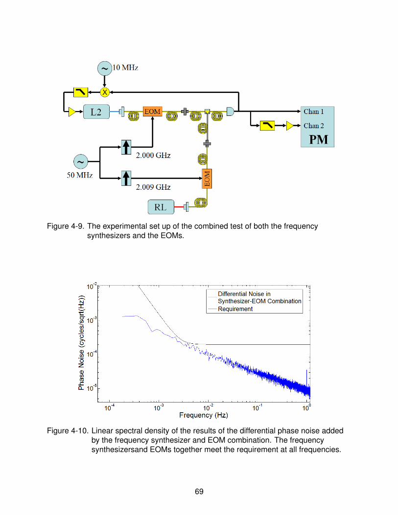
Figure 4-9. The experimental set up of the combined test of both the frequencysynthesizers and the EOMs.
Figure 4-10. Linear spectral density of the results of the differential phase noise addedby the frequency synthesizer and EOM combination. The frequencysynthesizersand EOMs together meet the requirement at all frequencies.
69
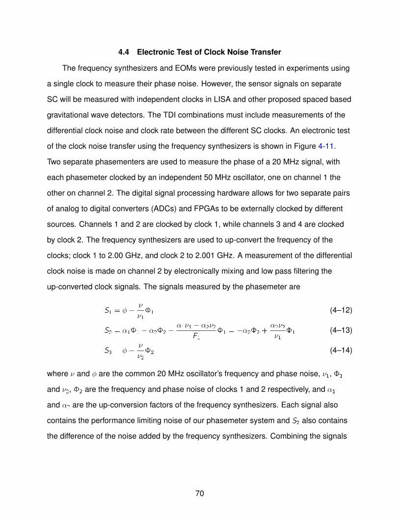
4.4 Electronic Test of Clock Noise Transfer
The frequency synthesizers and EOMs were previously tested in experiments using
a single clock to measure their phase noise. However, the sensor signals on separate
SC will be measured with independent clocks in LISA and other proposed spaced based
gravitational wave detectors. The TDI combinations must include measurements of the
differential clock noise and clock rate between the different SC clocks. An electronic test
of the clock noise transfer using the frequency synthesizers is shown in Figure 4-11.
Two separate phasementers are used to measure the phase of a 20 MHz signal, with
each phasemeter clocked by an independent 50 MHz oscillator, one on channel 1 the
other on channel 2. The digital signal processing hardware allows for two separate pairs
of analog to digital converters (ADCs) and FPGAs to be externally clocked by different
sources. Channels 1 and 2 are clocked by clock 1, while channels 3 and 4 are clocked
by clock 2. The frequency synthesizers are used to up-convert the frequency of the
clocks; clock 1 to 2.00 GHz, and clock 2 to 2.001 GHz. A measurement of the differential
clock noise is made on channel 2 by electronically mixing and low pass filtering the
up-converted clock signals. The signals measured by the phasemeter are
S1 = ϕ− ν
ν1�1 (4–12)
S2 = α1�1 − α2�2 −α1ν1 − α2ν2
F1
�1 = −α2�2 +α2ν2ν1
�1 (4–13)
S3 = ϕ− ν
ν2�2 (4–14)
where ν and ϕ are the common 20 MHz oscillator’s frequency and phase noise, ν1, �1
and ν2, �2 are the frequency and phase noise of clocks 1 and 2 respectively, and α1
and α2 are the up-conversion factors of the frequency synthesizers. Each signal also
contains the performance limiting noise of our phasemeter system and S2 also contains
the difference of the noise added by the frequency synthesizers. Combining the signals
70
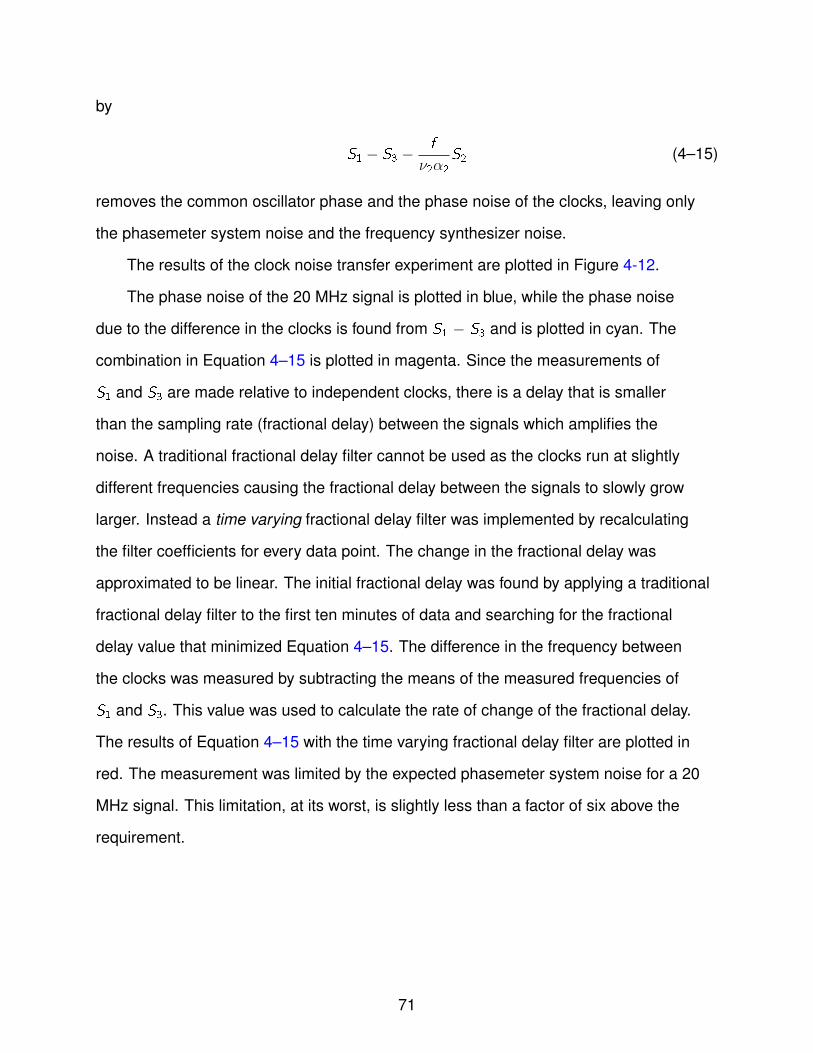
by
S1 − S3 −f
ν2α2
S2 (4–15)
removes the common oscillator phase and the phase noise of the clocks, leaving only
the phasemeter system noise and the frequency synthesizer noise.
The results of the clock noise transfer experiment are plotted in Figure 4-12.
The phase noise of the 20 MHz signal is plotted in blue, while the phase noise
due to the difference in the clocks is found from S1 − S3 and is plotted in cyan. The
combination in Equation 4–15 is plotted in magenta. Since the measurements of
S1 and S3 are made relative to independent clocks, there is a delay that is smaller
than the sampling rate (fractional delay) between the signals which amplifies the
noise. A traditional fractional delay filter cannot be used as the clocks run at slightly
different frequencies causing the fractional delay between the signals to slowly grow
larger. Instead a time varying fractional delay filter was implemented by recalculating
the filter coefficients for every data point. The change in the fractional delay was
approximated to be linear. The initial fractional delay was found by applying a traditional
fractional delay filter to the first ten minutes of data and searching for the fractional
delay value that minimized Equation 4–15. The difference in the frequency between
the clocks was measured by subtracting the means of the measured frequencies of
S1 and S3. This value was used to calculate the rate of change of the fractional delay.
The results of Equation 4–15 with the time varying fractional delay filter are plotted in
red. The measurement was limited by the expected phasemeter system noise for a 20
MHz signal. This limitation, at its worst, is slightly less than a factor of six above the
requirement.
71
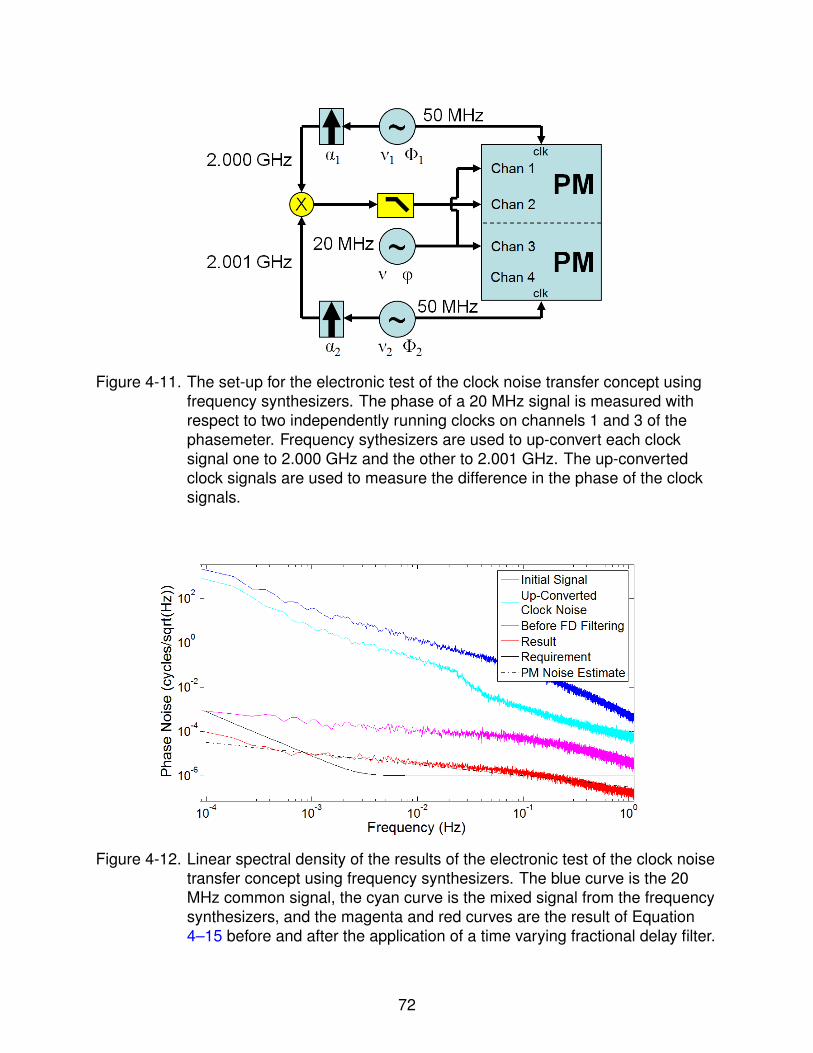
Figure 4-11. The set-up for the electronic test of the clock noise transfer concept usingfrequency synthesizers. The phase of a 20 MHz signal is measured withrespect to two independently running clocks on channels 1 and 3 of thephasemeter. Frequency sythesizers are used to up-convert each clocksignal one to 2.000 GHz and the other to 2.001 GHz. The up-convertedclock signals are used to measure the difference in the phase of the clocksignals.
Figure 4-12. Linear spectral density of the results of the electronic test of the clock noisetransfer concept using frequency synthesizers. The blue curve is the 20MHz common signal, the cyan curve is the mixed signal from the frequencysynthesizers, and the magenta and red curves are the result of Equation4–15 before and after the application of a time varying fractional delay filter.
72

CHAPTER 5DEVELOPMENT OF PSEUDO-RANDOM NOISE CODE RANGING
5.1 Delay-Locked Loop (DLL) Design
The PRN ranging technique described in Section 2.3.2 requires a digital delay-locked
loop (DLL) to track the received PRN code from the other SC. The photo detector
signal will contain a beat note between the received laser and the local laser in the
frequency range 2 to 20 MHz (as well as sideband beat notes). This signal will be phase
modulated with two Manchester-encoded PRN codes, one from the far SC and one
from the local SC. The ability of the DLL to track the PRN code from the far SC will be
limited by both the shot noise at the photo detector (at a level of 10−5cycles/√Hz) and
the interference from the local PRN code. The LISA science team has set a goal of 1
meter ranging accuracy [54]. Since the rate of change of the length of the LISA arms
can be well approximated as linear at any given time, it will be sufficient to require that
the ranging measurement be updated every 2 seconds (0.5 Hz bandwidth) and have a
root mean square error less than 1 meter. This section describes in detail the design
and predicted performance of the DLL.
5.1.1 Phasemeter Transfer Function
Figure 5-1 is a diagram of the delay-locked loop (DLL) and the phasemeter.
The phasemeter is used to measure the phase of the laser beat note and also to
demodulate the PRN code from the beat note. The phasemeter is designed to track
the phase fluctuations of the laser beat note at low frequencies. Inside the loop of the
phasemeter any low frequency signal is tracked and suppressed. The high frequency
PRN modulations will be outside the bandwidth of the phasemeter and hence will
be present before the loop filter as out of band noise. In this way the phasemeter
will demodulate the PRN signal from the beat note and serve as a high pass filter,
separating the high frequency PRN code from the low frequency laser phase noise. The
UFLIS phasemeter acts as a second order high pass filter with a 3 dB point at 10 kHz
73

Figure 5-1. Diagram of the LISA phasemeter and Delay-Locked Loop. The phasemetermeasures the phase of the laser beat note contained in the photo detectorsignal. The phasemeter is also used as a high pass filter, separating the highfrequency PRN code from the low frequency laser phase noise. Thedelay-locked loop (DLL) tracks the changes in the arrival time of theincoming PRN code caused by the SC motion.
[52]. We will model its transfer function as
(f /10kHz)2
1 + (f /10kHz)2(5–1)
The shot noise that enters the measurement at the photo detectors will also be high
pass filtered by the phasemeter transfer function.
In principle, the PRN code is also filtered by the phasemeter transfer function [60].
However, as our phasemeter has only a bandwidth of 10 kHz, this effect is negligible.
5.1.2 Filtering the Double Frequency Term
After the multiplication between the local oscillator and the photo detector signal
(Figure 5-1) the PRN code has been removed from the phase of the carrier, but
the multiplication results in a frequency doubled (2ν) term. This term is at twice the
frequency of the measured beat note. In most spread spectrum applications the carrier
frequency would be much higher than the PRN chip rate (100s of MHz to GHz) [61].
Thus the 2ν term could easily be removed with a low pass filter. In LISA, however,
74

the beat notes will range from 2 to 20 MHz creating 2ν terms from 4 to 40 MHz.1
The Manchester encoded PRN contains a significant amount of information at these
frequencies making low pass filtering impossible without distorting the received PRN
code. Instead a time domain filter was designed to mitigate the 2ν term.
Figure 5-2 is a diagram of the filter to remove the 2ν term. A third local oscillator is
programmed to create a sinusoid that runs at twice the rate of the local oscillator. This
signal is multiplied by the in-phase (I) component so that its amplitude matches the 2ν
term. This signal is then subtracted from the quadrature (Q) component before the low
pass filter. The photo detector signal is modeled as
PD = A(t)sin [2πνt + ϕ(t) + βPRN(t)] (5–2)
where A(t) is the amplitude of the beat note, ν is the frequency, ϕ(t) is the phase noise
including both laser noise and shot noise, β is the amplitude of the modulated PRN
code (in radians), and PRN(t) is the PRN code. The phase noise can be split into
frequency components that are inside and outside the bandwidth of the phasemeter;
ϕ(t) = ϕib(t) + ϕob(t). The signals from the local oscillators are
cos [2πνt + ϕib(t)] (5–3)
sin [4πνt + 2ϕib(t)] (5–4)
sin [2πνt + ϕib(t)] (5–5)
1 There are currently several competing space based gravitational wave detectordesigns. Many of these designs involve changes to the SC orbits which would lead toa different range of beat note frequencies due to the Doppler shift. It is possible that thechosen design will include beat note frequencies lower than 2 MHz
75
After multiplication of the cosine term with the photo detector signal, the quadrature term
before the low pass filter is
QHF (t) = A(t) [ϕob(t) + βPRN(t) + sin [4πνt + 2ϕib(t) + ϕob(t) + βPRN(t)]] (5–6)
After low pass filtering the in phase component (I(t)) is simply equal to the amplitude
A(t). The signal to be sent to the DLL is formed by
DLL(t) = (QHF (t)− A(t)sin [4πνt + 2ϕib(t)]) /A(t)
DLL(t) =ϕob(t) + βPRN(t)
+ 2sin
[ϕob + βPRN(t)
2
]cos
[4πνt + 2ϕib(t) +
1
2ϕob(t) +
1
2βPRN(t)
]The double frequency term has been attenuated by 2sin
[ϕob+βPRN(t)
2
]≈ ϕob + βPRN(t).
Figure 5-3 is a plot of a simulation of the signal to be sent to the DLL with and without
this filter in the case of a beat note at 2 MHz. The filter results in reduction of the double
frequency term by roughly a factor of 20.
Figures 5-4, 5-5, and 5-6 are the results of nine simulations to measure the error
signal formed with and without the filter to remove the double frequency term. The
simulation was run for beat note frequencies of 1, 2, 2.5, 3, 5, 10, 13.5, 15, and 20 MHz.
The simulation was run with a constant beat note frequency and with no phase noise.
The error signal was measured by performing a correlation of the received code with an
early and late version of the same code (separated by half a chip) and subtracting those
correlations. The correlation was made over the entire length of the code. The relative
delay between the local codes and the received code was shifted between ±50 samples.
The shape of the measured signal depends on the frequency of the 2ν term and
its phase with respect to the received PRN code. Since the both the frequency and
phase of the beat note will drift over time during the actual LISA mission, the effect of
the 2ν term on the error signal will be time varying and unpredictable. Since the DLL will
serve to drive the error signal to zero it is of particular importance to ensure that the zero
76

Figure 5-2. Phasemeter with filter to remove the 2ν term. The filter works by using thephasemeter feedback to generate a signal with twice the frequency ofmeasured beat note and subtracting this signal from the quadrature signal.The amplitude of the beat note is also measured and used to appropriatelyscale the generated double frequency term before the subtraction. Themeasured amplitude is also used as automatic gain control to ensure thatthe received PRN code has the same amplitude before being sent to theDLL regardless of the amplitude of the measured beat note.
crossing of the error signal is within 3 ns of the true zero, as 3 ns corresponds to a light
travel distance of 1 meter. A requirement of 0.5 meters was set on both the zero point
crossing and the root mean square error of all correlations within the locking region.
The error signals formed with the 2ν filter were excellent in zero crossing and root
mean square error. For all of the beat note frequencies greater than or equal to 3 MHz
the zero crossing point of the error signals was within ±0.005 samples (0.03 m) of
the true zero and root mean square error of all points in the locking region was within
±0.008 samples (0.048 m) of the expected values. For the beat notes less than 3 MHz
the zero crossing points were within ±0.05 samples (0.3 m) and the root mean square
error of all points in the locking region was within ±0.01 samples (0.06 m).
77

Figure 5-3. Graph of the received PRN code after demodulation from the carrier withand without the subtraction to remove the 2ν term. The 2ν filter results in anattenuation of the 2ν term by a factor of approximately 20.
The error signals formed without the 2ν filter were unacceptable for all the simulated
beat note frequencies except 3, 5, and 20 MHz. At 3, 5, and 20 MHz the zero crossing
points were within ±0.05 samples (0.3 m) and the root mean square error in the locking
region was within ±0.07 samples (0.46 m). For all other frequencies the zero crossing
ranged from ±0.25 samples (1.5 m) to ±1.4 samples (8.4 m) and the root mean square
error in the locking region ranged from ±0.24 samples (1.44 m) to ±1.96 samples (11.76
m).
The 2ν filter will allow the error signal to be formed without correction while the beat
note continuously moves between frequencies of 2 to 20 MHz.
78

Figure 5-4. Error Signals with and without the 2ν filter at beat note frequencies of 1, 2,and 2.5 MHz.
79
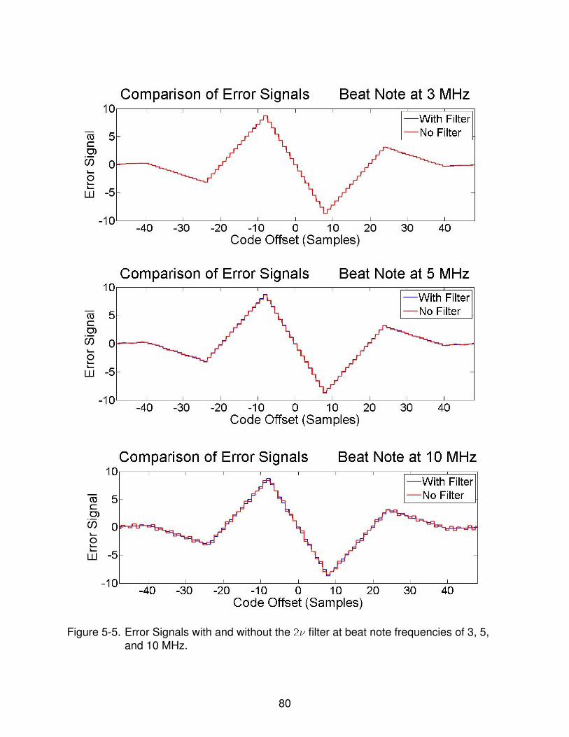
Figure 5-5. Error Signals with and without the 2ν filter at beat note frequencies of 3, 5,and 10 MHz.
80
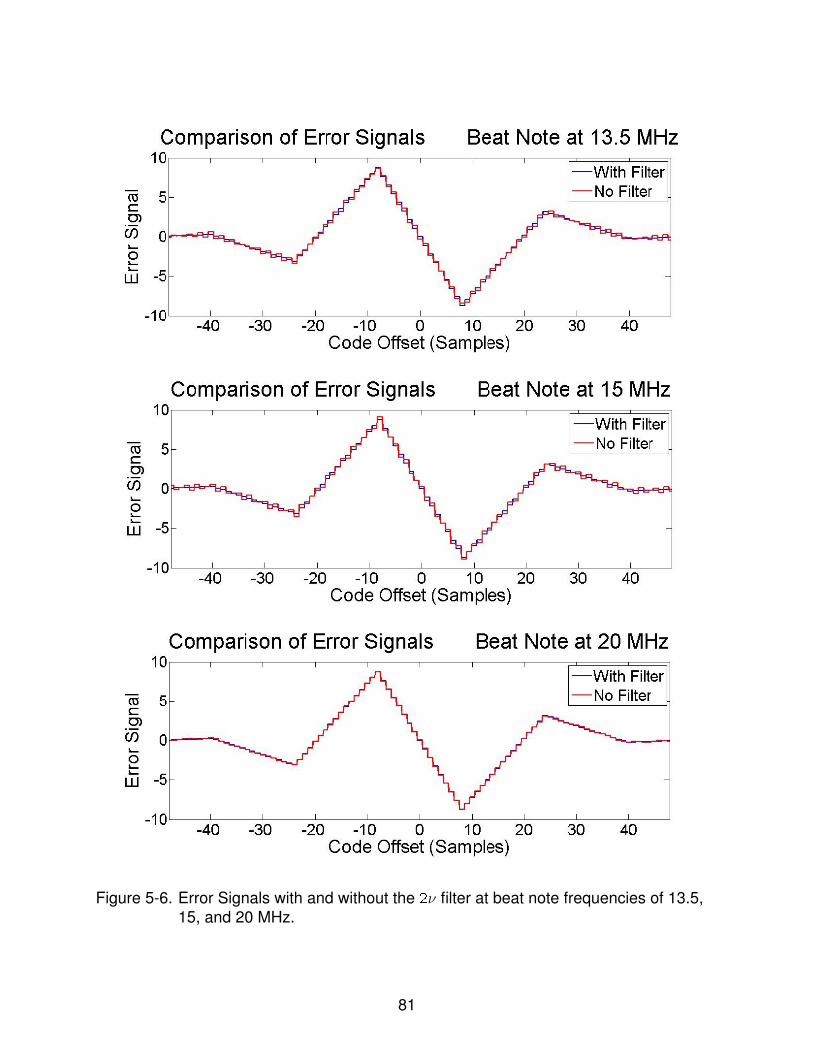
Figure 5-6. Error Signals with and without the 2ν filter at beat note frequencies of 13.5,15, and 20 MHz.
81

5.1.3 Linearized Delay-Locked Loop Model
Figure 5-7 is a diagram of the DLL.2 The input to the DLL can be written as
βPRN(t − T ) + n(t) (5–7)
where β is the amplitude of the PRN code (in radians), T is the time offset of the
received PRN code, and n(t) is the sum of all noise sources, including the out of band
phase noise from the phasemeter, the local PRN code, and the double frequency term.
An error signal can be formed by correlating the received PRN code with an early and
late version of the same code, and then subtracting the two correlations (Figure 5-8).
Error(t,T , T ) = PRN(t − T ) · PRN(t − T − �T )− PRN(t − T ) · PRN(t − T + �T )
(5–8)
Where T is the time offset of the locally generated signals and �T is the timing offset of
the early and late codes. The digital signal processing can be simplified by subtracting
the early and late PRN codes before correlating.
EL(T − T ) = PRN(t − T − �T )− PRN(t − T + �T ) (5–9)
A half chip delay between the early and late codes was chosen as this maximizes
the slope of the locking region of the error signal (Figure 5-8). The output of the
multiplication is written as
[βPRN(t − T ) + n(t)] · EL(T − T ) = βD(T − T ) + βN(t,T , T ) + n(t)EL(T − T )
(5–10)
2 The analysis in this section follows Chapter 9-4 in Digital Communications andSpread Spectrum Systems by Ziemer and Peterson [62].
82

Figure 5-7. The Delay-Locked Loop. An error signal is created by multiplying thereceived PRN code by the difference between and early and late (timedelayed and time advanced) version of the same code. The DC portion ofthe multiplication, βD(T − T ), provides the error signal to the loop and isequivalent to the correlation of the PRN code with the early-late subtraction.
where D(T − T ) and N(t,T , T ) are the DC and AC components of the product of
PRN(t − T ) and EL(T − T ), and n(t) is the noise from the phasemeter output.
D(T − T ) is plotted as the error signal in Figure 5-8 because the DC component of
the product of two signals is equivalent to their correlation. The AC part of the multiplier
output, N(t,T , T ), is known as the code self-noise. The effect of n(t) and the code
self-noise on the DLL tracking is considered in Section 5.1.5.
While the local early-late code is locked to the incoming code, the error signal
D(T − T ) is confined to the locking region between plus and minus one quarter chip
(Figure 5-8). In this region D(T − T ) = 316(T − T ). Thus a linearized model of the
delay-locked loop will be valid as long as the tracking error, (T − T ), stays within plus
and minus one quarter chip. Figure 5-9 is the linearized version of the DLL where T ,
the arrival time of the received code, is the input to the loop, T is the output of the
control loop, and the multiplier is replaced by a subtractor. This leads to an error signal
of (T − T ). This is different from the value in Equation 5-8, which is βS(T − T ).
Inside the actual DLL the signal to be tracked is scaled by βS , the amplitude of the PRN
code times the slope of the error signal, but the noise is not. To account for this in the
83
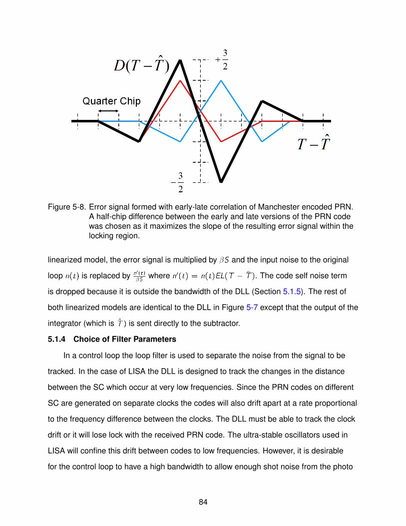
Figure 5-8. Error signal formed with early-late correlation of Manchester encoded PRN.A half-chip difference between the early and late versions of the PRN codewas chosen as it maximizes the slope of the resulting error signal within thelocking region.
linearized model, the error signal is multiplied by βS and the input noise to the original
loop n(t) is replaced by n′(t)βS
where n′(t) = n(t)EL(T − T ). The code self noise term
is dropped because it is outside the bandwidth of the DLL (Section 5.1.5). The rest of
both linearized models are identical to the DLL in Figure 5-7 except that the output of the
integrator (which is T ) is sent directly to the subtractor.
5.1.4 Choice of Filter Parameters
In a control loop the loop filter is used to separate the noise from the signal to be
tracked. In the case of LISA the DLL is designed to track the changes in the distance
between the SC which occur at very low frequencies. Since the PRN codes on different
SC are generated on separate clocks the codes will also drift apart at a rate proportional
to the frequency difference between the clocks. The DLL must be able to track the clock
drift or it will lose lock with the received PRN code. The ultra-stable oscillators used in
LISA will confine this drift between codes to low frequencies. However, it is desirable
for the control loop to have a high bandwidth to allow enough shot noise from the photo
84

Figure 5-9. Linearized version of the Delay-Locked Loop. The extra factor of βS is addedto the model and the input noise is replaced with n′(t)
βS. This is done so that
the error signal has the same amplitude as in Equation 5–10.
detector to dither the DLL output between samples Section 5.1.6). A 1 kHz bandwidth
was selected to allow for sufficient dithering to achieve sub meter precision, to reject
enough noise to ensure that the control loop doesn’t lose lock, and to attenuate all code
self-noise terms in the loop.
The DLL contains an integrator which contributes a 1/f dependence to the open
loop transfer function. Since the signal to be tracked (the motion of the SC and the drift
due to clock differences) varies slowly it was decided that the 1/f dependence of the
integrator would be sufficient at low frequencies for tracking. To further suppress the
noise at high frequencies the loop filter was chosen to be a single pole low pass filter
with 3 dB point at 1 kHz. The digital implementation of a single pole low pass filter is
shown is Figure 5-10. The parameter α determines the 3 dB point by
α =TS
1/2πf3dB + TS
(5–11)
where TS is the sample time and f3dB is the desired 3 dB frequency. This leads to
α = 1.2565 × 10⁻⁴. In order to run the DLL at a rate of 50 MHz on the FPGA the
arithmetic must be made as simple as possible. To do so all multiplications are rounded
85

Figure 5-10. Digital implementation of a single pole low pass filter.
to powers of two and replaced by bit shifting. The nearest power of two to α is 2−13 =
1.2207× 10⁻⁴. This leads to a 3 dB point of 972 Hz.
The scaling factor K in the loop (Figure 5-7 and 5-9) is chosen such that the rest
of the loop has its unity gain frequency where the low pass filter has its 3 dB point. This
way the open loop transfer function has a 1/f dependence in the loop bandwidth (below
1 kHz) and a 1/f 2 dependence outside of the loop bandwidth (above 1 kHz). This
requires that K = α/βS = 4.603× 10⁻³ ≈ 2−8 = 3.906× 10⁻³.
5.1.5 Noise Term Analysis
The tracking error will be determined by the noise n′(t)/βS that enters the
linearized version of the loop. The noise has four terms; the code self noise, the out of
band phase noise from the phasemeter, the local PRN signal, and the double frequency
term. The last three terms are all multiplied by the early-late subtraction. In Section
5.1.2 it was shown by simulation that with the 2ν filter the double frequency term has
a negligible effect on the error signal. Therefore it will be ignored in the tracking error
analysis.
The code self noise is given by the AC part of the product of the received PRN
code, and the early-late subtraction. Both the PRN code and the early-late subtraction
are periodic in the length of the code NTS . Thus the lowest possible non DC frequency
component of their product is 1/NTS = 1.526kHz . The bandwidth of the DLL is lower
than this frequency so the code self-noise can be ignored in the tracking analysis.
86

5.1.5.1 Phasemeter Out of Band Noise
The out of band noise from the phasemeter will be dominated by shot noise
at the photo detector. Shot noise is a white noise, in that it is uniformly spread
over all frequencies. The shot noise will have a spectral density of approximately
10µcycles/√Hz . The out of band noise from the phasemeter will not be white noise as
it will be high pass filtered by the phasemeter transfer function (Equation 5.1.1). The
frequency spectrum of the product of the out of band phase noise and the early-late
subtraction is given by the convolution of their Fourier transforms.
ϕ′(t) = ϕob(t) · EL(t) → ~ϕ′(ν) = ~ϕob(ν) ∗ ~EL(ν) =
∫ −∞
∞~ϕob(ν
′) ~EL(ν ′ − ν)dν ′ (5–12)
Since the early-late subtraction is periodic its frequency spectrum can be written as the
sum of delta functions. Thus
~ϕob(ν) =
∫ −∞
∞~ϕob(ν
′)∑k
Akδ(ν′ − νk − ν)dν ′ (5–13)
Pulling the sum outside of the integral and integrating over the delta functions gives
~ϕ′(ν) =∑k
Ak~ϕob(ν − νk) (5–14)
Since the frequency spectrum of the out of band noise is not band limited the
repeated spectrums will overlap. The components of the early-late subtraction span over
MHz (from 1.5 kHz to the Nyquist frequency, 25 MHz), while the notch in the out of band
noise is only 10 kHz wide. Thus it can be approximated to be white (|ϕob(ν)| = |ϕob|).
Therefore ~ϕ′(ν) is the sum of white noise terms scaled by Ak . These white noise terms
add quadratically ∣∣∣~ϕ′(ν)∣∣∣ = ∣∣∣~ϕob∣∣∣√∑
k
A2k (5–15)
This is simply equal to the amplitude of the out of band noise frequency spectrum times
the variance of the early-late subtraction (which is√3). Thus the contribution to the
87

noise term n′(t) from the out of band noise is white noise at the level of the shot noise
times√3. The phasemeter output to the DLL is scaled in radians and the values in the
DLL are interpreted in sample times (samples), so the expected out of band noise level
to the DLL is√310−5 cycles√
Hz2π
rad
cycle=
√3 · 2π10−5 samples√
Hz(5–16)
The noise can also be scaled from samples to meters as the sample time is 20 ns and
light travels 6 meters in that time.
6√3 · 2π10−5meters√
Hz= 6.5× 10⁻⁴meters√
Hz(5–17)
Inside the loop this noise is scaled by 1/βS ≈ 37.7 leading to a shot noise limitation
of 0.025meters/√Hz . Limiting the measurement to a bandwidth of 0.5 Hz leads to a root
mean square error of 0.017 meters.
5.1.5.2 Local PRN code Interference
The local PRN code will interfere with the tracking of the incoming code. If the
incoming code were not drifting due to the motion of the SC or due to the clock
frequency offsets, then the interference of the local PRN code would result in a small
DC offset to the error signal plus more AC code self noise terms. The code self noise
terms will be outside the bandwidth of the loop and the small DC offset would result in a
constant error in the measured pseudo range. In LISA, however, the tracking code will
follw the changing arrival time of the incoming code. This will cause the outgoing code to
drift with respect to the tracking code.
The codes used in this thesis have been designed to minimize their cross
correlation [48]. Figure 5-11 displays the amplitude of the DC portion of the error
signal formed by multiplying code 2 with the early-late tracking signal of code 1. This
was computed for 3050 consecutive sample differences between the codes. The
amplitude displayed is the expected error signal for a code modulated at β = 0.14rad
(one percent optical power). The early-late code will track the incoming code causing
88
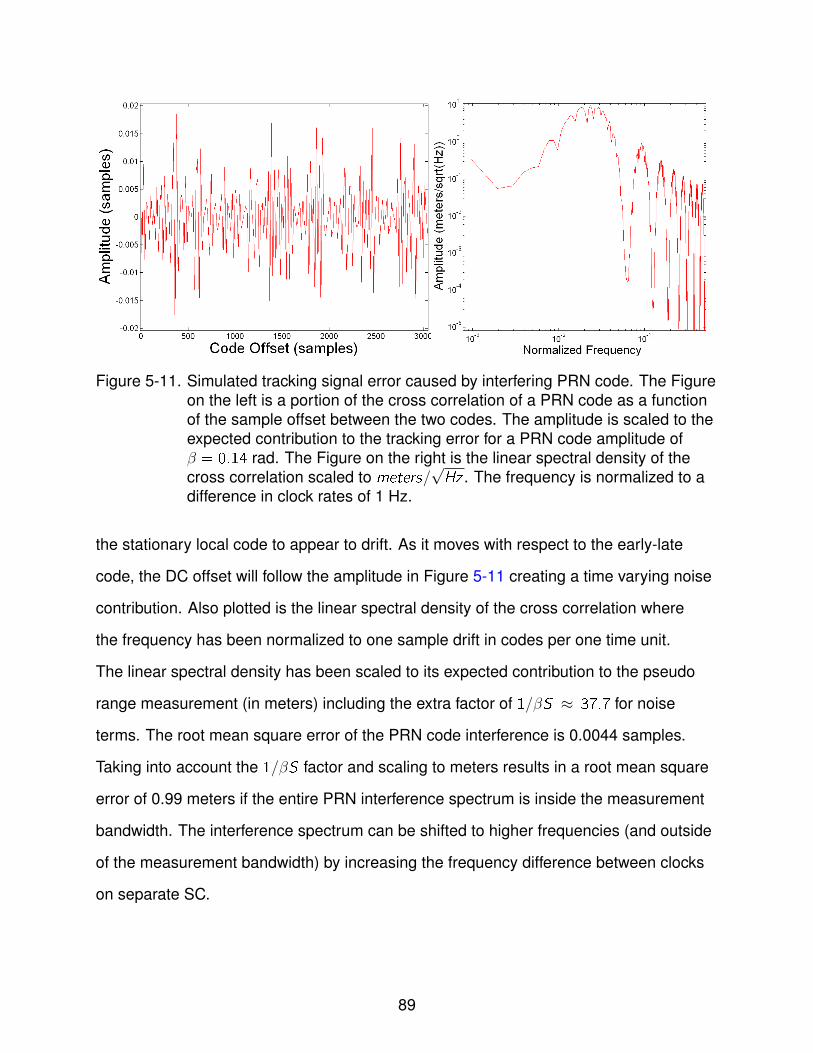
Figure 5-11. Simulated tracking signal error caused by interfering PRN code. The Figureon the left is a portion of the cross correlation of a PRN code as a functionof the sample offset between the two codes. The amplitude is scaled to theexpected contribution to the tracking error for a PRN code amplitude ofβ = 0.14 rad. The Figure on the right is the linear spectral density of thecross correlation scaled to meters/
√Hz . The frequency is normalized to a
difference in clock rates of 1 Hz.
the stationary local code to appear to drift. As it moves with respect to the early-late
code, the DC offset will follow the amplitude in Figure 5-11 creating a time varying noise
contribution. Also plotted is the linear spectral density of the cross correlation where
the frequency has been normalized to one sample drift in codes per one time unit.
The linear spectral density has been scaled to its expected contribution to the pseudo
range measurement (in meters) including the extra factor of 1/βS ≈ 37.7 for noise
terms. The root mean square error of the PRN code interference is 0.0044 samples.
Taking into account the 1/βS factor and scaling to meters results in a root mean square
error of 0.99 meters if the entire PRN interference spectrum is inside the measurement
bandwidth. The interference spectrum can be shifted to higher frequencies (and outside
of the measurement bandwidth) by increasing the frequency difference between clocks
on separate SC.
89
5.1.6 Rounding of Tracking Code Delay
While the incoming PRN code can be delayed by any value T, the early-late tracking
code delay T can only be varied in integer steps of the sample time TS = 20ns.
The feedback of the DLL will only activate if the control signal reaches ±0.5samples.
Otherwise it will be rounded to zero. This could happen if the incoming code is
stationary and the input noise to the DLL is sufficiently small. Since the control loop
won’t be activated, the noise will be acted upon by the open loop transfer function.
However, since the noise is integrated inside the loop, after a time τ the control
signal will reach ±0.5samples, and the closed loop transfer function will take over at
frequencies below f0 = 1/τ . This frequency can be estimated by assuming that the
tracking will begin once the variance squared of the tracking error reaches some critical
value σ2. As the variance squared is equal to the area under the power spectral density,
this will happen when
σ2 =A2
(βS)2
∫ ∞
f0
1
(f /1kHz)2 + (f /1kHz)4df (5–18)
where A is the amplitude of the linear spectral density of the shot noise and the function
under the integral is the open loop transfer function of the DLL. If the amplitude, A, of the
noise is sufficiently large, f0 will be bigger than 1 kHz and Equation 5–18 can be taken
as
σ2 ≈ A2
(βS)2
∫ ∞
f0
(1kHz
f
)4
df (5–19)
Integrating and solving for f0 results in
f0 =3
√(A/βS)2 · 1kHz
3σ2· 1kHz (5–20)
where
A >
√3(βS)2σ2
1kHzto have f0 > 1kHz (5–21)
90
If A is smaller than this value, Equation 5–18 can be approximated as
σ2 ≈ A2
(βS)2
[∫ 1kHz
f0
(1kHz
f
)2
df +
∫ ∞
1kHz
(1kHz
f
)4
df
](5–22)
Integrating results in
σ2 =
(A
βS
)2(1kHz
f0− 2
3
)1kHz (5–23)
Solving for f0 results in
f0 =
(σ2(βS)2
A2kHz+
2
3
)−1
1kHz (5–24)
where
A <
√3(βS)2σ2
1kHz(5–25)
The incoming code will not necessarily arrive at one of the integer steps of the
early-late tracking code. If the incoming code delay T is near the midpoint between
integer steps of the early-late tracking code delay T , then even the smallest variations
due to the noise will cause the control signal to be rounded ahead or behind (Figure
5-12). This will act as an additional amplification within the loop leading to a higher
bandwidth than would otherwise be expected.
In LISA the incoming PRN code will not be stationary because the distance
between the SC will be changing and the PRN codes will be generated on separate
clocks. A frequency difference of f Hz between the clocks will lead to an f sample per
second drift between the two codes.
5.2 Delay-Locked Loop Simulations
Two computer simulations were performed to verify the above tracking analysis. The
simulations were run in the Matlab Simulink environment with the same DLL design to
be programmed in hardware. A 5 MHz beat note was simulated with an amplitude of
0.15 relative to the full voltage range of the ADCs, a Manchester Encoded PRN at an
91

Figure 5-12. Diagram of two possible relative positions between the delay of theincoming PRN code and the early-late tracking code.
amplitude of 0.14 rad, and simulated white noise at 1µcycles/√Hz in one simulation and
10µcycles/√Hz in the other. The phasemeter was programmed with the 2ν filter and the
PRN amplitude control. All of the operations in the simulation use the same fixed-point
precision as the hardware version of the DLL and phasemeter. The simulations were
each run twice, once for a million samples while recording data at the simulated sample
rate of 50 MHz, and once for 100 million samples while recording data at a down
sampled rate of 50MHz/1024 = 49kHz . CIC filters were used to prevent aliasing into
the down sampled data. These sample times correspond to measurement times of 0.02
and 2 seconds respectively. Since the simulation can’t simulate fractional delays in the
arrival time of the incoming code the incoming PRN code is simulated to arrive right at
an integer multiple of the tracking code. The incoming code is also stationary as the
simulation must use the same data rate for everything in the simulation.
The result of the first simulation (noise level 1µcycles/√Hz) is plotted in Figure 5-13.
Three signals are plotted, the output of the phasemeter to the DLL (Figure 5-1), the error
signal formed after multiplication of the input signal with the early-late tracking code,
and the output of the DLL which is the pseudo range. All of these signals are scaled
to meters/√Hz . The noise from the phasemeter output is low enough that the spread
92

Figure 5-13. Linear spectral density of the results of the DLL tracking simulation withwhite noise at 1 µcycles/
√Hz . The output of the phasemeter to the DLL is
plotted in blue, the error signal formed inside the DLL is plotted in magenta,and the noise in the measured pseudo range is plotted in green. The lowlevel of the input noise causes the measured pseudo range to follow theopen loop transfer function of the DLL at frequencies above 10 Hz.
spectrum of the PRN code can clearly be seen. Also shown is the linear spectral density
of the error signal. It fits well with the estimated level of 6.5 × 10⁻⁴meters/√Hz from
Equation 5–17. Since there is no variation of the pseudo range that is supposed to be
measured, the DLL output is the tracking error. The noise is dominated by the rounding
effect dicsussed in Section 5.1.6. The tracking error follows very closely to the open loop
transfer function times the estimated noise level. The feedback loop doesn’t start to take
effect until the very end of the plotted spectrum around 10 Hz. Using Equation 5–24
and choosing σ2 = 0.02 results in f0 = 8.1Hz and a tracking error of 0.3meters/√Hz at
frequencies below f0.
The result of the second simulation (noise level 10µ cycles√Hz
) is plotted in Figure
5-14. The noise from the phasemeter output is high enough that only the very tip of
the spread spectrum of the PRN code can be seen around 1 MHz. Also shown is
93
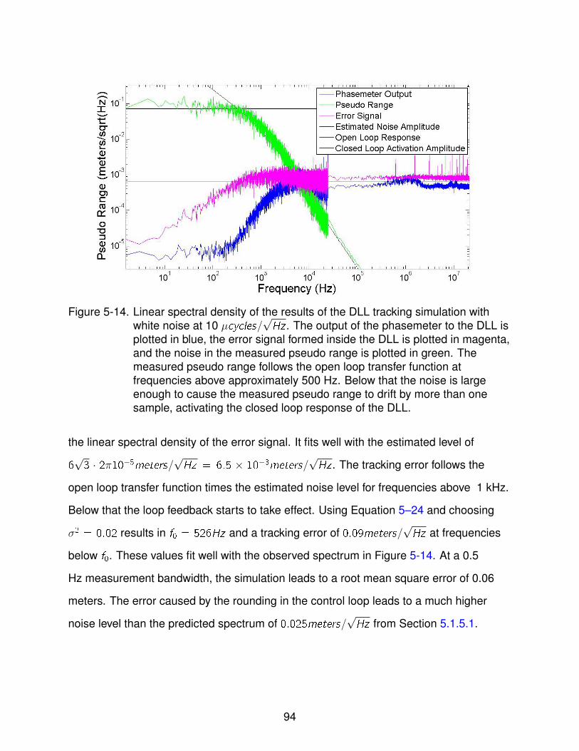
Figure 5-14. Linear spectral density of the results of the DLL tracking simulation withwhite noise at 10 µcycles/
√Hz . The output of the phasemeter to the DLL is
plotted in blue, the error signal formed inside the DLL is plotted in magenta,and the noise in the measured pseudo range is plotted in green. Themeasured pseudo range follows the open loop transfer function atfrequencies above approximately 500 Hz. Below that the noise is largeenough to cause the measured pseudo range to drift by more than onesample, activating the closed loop response of the DLL.
the linear spectral density of the error signal. It fits well with the estimated level of
6√3 · 2π10−5meters/
√Hz = 6.5 × 10⁻³meters/
√Hz . The tracking error follows the
open loop transfer function times the estimated noise level for frequencies above 1 kHz.
Below that the loop feedback starts to take effect. Using Equation 5–24 and choosing
σ2 = 0.02 results in f0 = 526Hz and a tracking error of 0.09meters/√Hz at frequencies
below f0. These values fit well with the observed spectrum in Figure 5-14. At a 0.5
Hz measurement bandwidth, the simulation leads to a root mean square error of 0.06
meters. The error caused by the rounding in the control loop leads to a much higher
noise level than the predicted spectrum of 0.025meters/√Hz from Section 5.1.5.1.
94
5.3 Optical Delay-Locked Loop Tests
Figure 5-15 is a diagram of the experimental set up to test the ranging capabilities
of the DLL using LISA-like hardware. The set up utilizes the optical configuration of
UFLIS to produce a laser beat note between the cavity stabilized reference laser and
laser 2. Laser 2 is phase locked to the reference laser with an analog phase lock loop
offset by 5 MHz. In order to increase the noise present at the photo detector to LISA like
levels, Laser 2 was attenuated by misalignment in the optical fiber. The photo detector
output is amplified three times (Texas Instruments SLOP231 THS4022) to produce a
large enough signal for the phasemeter.
The phasemeter-DLL system was programmed on the input daughter card while
the outgoing PRN code was programmed on the output daughter card of the digital
signal processing system described in Section 3.5. Two such systems were used, one
outputting code 1 and the other code 2. The digital signal processing systems could be
set up to run on separate clocks (as shown) or on the same clock.
The EOMs were modulated with the PRN codes so that one percent of the power
was in the spread spectrum. The half wave voltage of the EOMs is Vπ = 6V . To produce
a modulation with one percent of the power in the spread spectrum the modulation must
be at 0.14rad . This happens at a voltage of V = 0.14π6V = 267mV .
The EOMs used in the experiment are designed for much greater than 100 pW laser
power. Thus the noise present at the photo detectors is not shot noise, but is electronic
noise associated with the photo detector’s amplifier and the three additional amplifiers.
The measurements in Chapter 5 were performed at two noise levels, one at a targeted
level of 1µcycles/√Hz and the other at a targeted level of 10µcycles/
√Hz . The level of
the phase noise was measured by using the signal to noise ratio of the amplified beat
note recorded on a spectrum analyzer (Advantest R3131A).
95
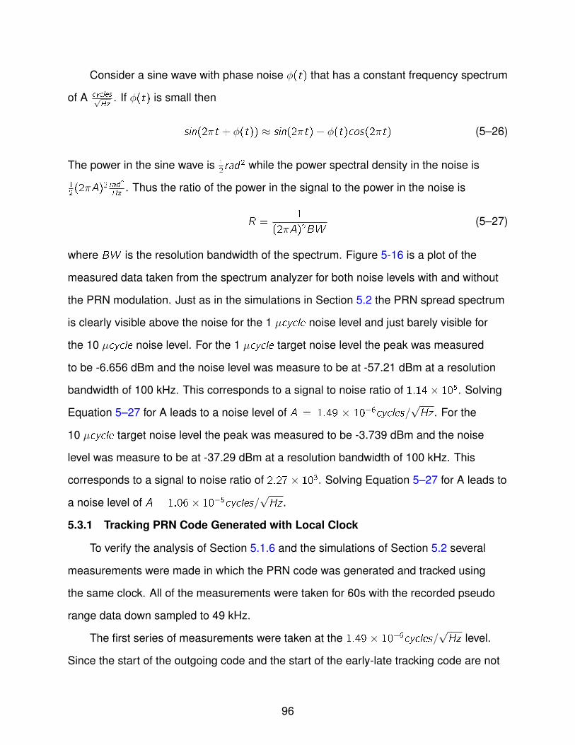
Consider a sine wave with phase noise ϕ(t) that has a constant frequency spectrum
of A cycles√Hz
. If ϕ(t) is small then
sin(2πt + ϕ(t)) ≈ sin(2πt) + ϕ(t)cos(2πt) (5–26)
The power in the sine wave is 12rad2 while the power spectral density in the noise is
12(2πA)2 rad
2
Hz. Thus the ratio of the power in the signal to the power in the noise is
R =1
(2πA)2BW(5–27)
where BW is the resolution bandwidth of the spectrum. Figure 5-16 is a plot of the
measured data taken from the spectrum analyzer for both noise levels with and without
the PRN modulation. Just as in the simulations in Section 5.2 the PRN spread spectrum
is clearly visible above the noise for the 1 µcycle noise level and just barely visible for
the 10 µcycle noise level. For the 1 µcycle target noise level the peak was measured
to be -6.656 dBm and the noise level was measure to be at -57.21 dBm at a resolution
bandwidth of 100 kHz. This corresponds to a signal to noise ratio of 1.14 × 10⁵. Solving
Equation 5–27 for A leads to a noise level of A = 1.49 × 10⁻⁶cycles/√Hz . For the
10 µcycle target noise level the peak was measured to be -3.739 dBm and the noise
level was measure to be at -37.29 dBm at a resolution bandwidth of 100 kHz. This
corresponds to a signal to noise ratio of 2.27× 10³. Solving Equation 5–27 for A leads to
a noise level of A = 1.06× 10⁻⁵cycles/√Hz .
5.3.1 Tracking PRN Code Generated with Local Clock
To verify the analysis of Section 5.1.6 and the simulations of Section 5.2 several
measurements were made in which the PRN code was generated and tracked using
the same clock. All of the measurements were taken for 60s with the recorded pseudo
range data down sampled to 49 kHz.
The first series of measurements were taken at the 1.49 × 10⁻⁶cycles/√Hz level.
Since the start of the outgoing code and the start of the early-late tracking code are not
96
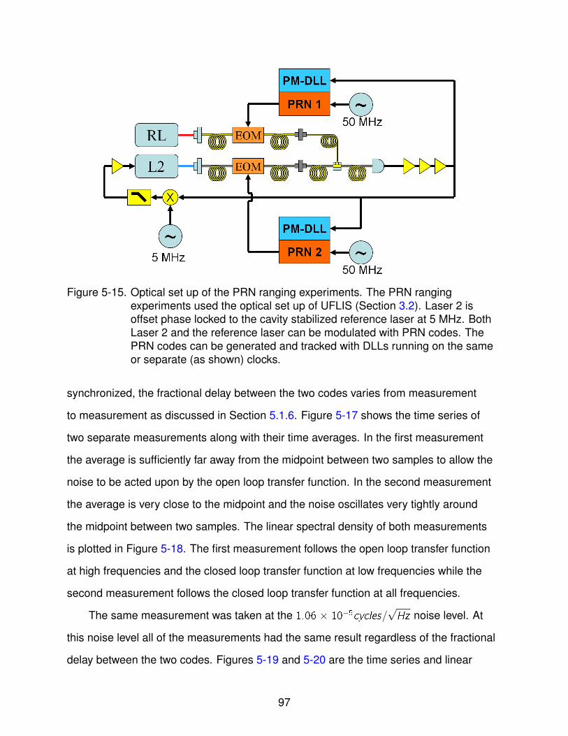
Figure 5-15. Optical set up of the PRN ranging experiments. The PRN rangingexperiments used the optical set up of UFLIS (Section 3.2). Laser 2 isoffset phase locked to the cavity stabilized reference laser at 5 MHz. BothLaser 2 and the reference laser can be modulated with PRN codes. ThePRN codes can be generated and tracked with DLLs running on the sameor separate (as shown) clocks.
synchronized, the fractional delay between the two codes varies from measurement
to measurement as discussed in Section 5.1.6. Figure 5-17 shows the time series of
two separate measurements along with their time averages. In the first measurement
the average is sufficiently far away from the midpoint between two samples to allow the
noise to be acted upon by the open loop transfer function. In the second measurement
the average is very close to the midpoint and the noise oscillates very tightly around
the midpoint between two samples. The linear spectral density of both measurements
is plotted in Figure 5-18. The first measurement follows the open loop transfer function
at high frequencies and the closed loop transfer function at low frequencies while the
second measurement follows the closed loop transfer function at all frequencies.
The same measurement was taken at the 1.06 × 10⁻⁵cycles/√Hz noise level. At
this noise level all of the measurements had the same result regardless of the fractional
delay between the two codes. Figures 5-19 and 5-20 are the time series and linear
97

Figure 5-16. Measured power spectral densities of amplified laser beat signals with andwithout PRN code for different noise levels. For the µcycle/
√Hz noise level
the PRN code generates broad sidebands around the carrier beat. Thesedisappear if the noise is increased to 10µcycle/
√Hz .
Figure 5-17. Time series of measured pseudo ranges with 1µcycle/√Hz noise level
using the same clock to generate and track the PRN code. In the graph onthe left the arrival of the incoming code is sufficeintly far away from amidpoint between two samples of the local clock. This allows the measuredpseudo range to drift for a significant amount of time before being thefeedback to the local code is rounded up or down. In the graphs on theright the arrival of the incoming code is very near to a midpoint betweensamples of the local clock. This causes the feedback to the local code tooscillate rapidly between a half sample ahead and behind the incomingcode.
98
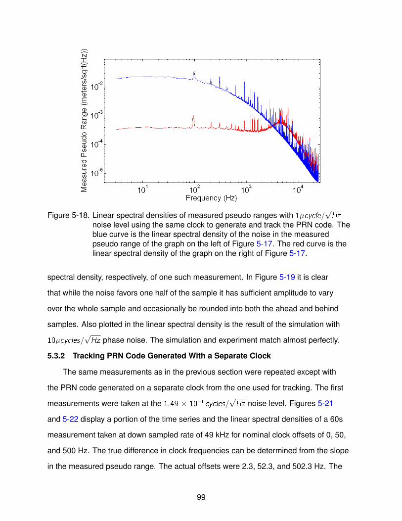
Figure 5-18. Linear spectral densities of measured pseudo ranges with 1µcycle/√Hz
noise level using the same clock to generate and track the PRN code. Theblue curve is the linear spectral density of the noise in the measuredpseudo range of the graph on the left of Figure 5-17. The red curve is thelinear spectral density of the graph on the right of Figure 5-17.
spectral density, respectively, of one such measurement. In Figure 5-19 it is clear
that while the noise favors one half of the sample it has sufficient amplitude to vary
over the whole sample and occasionally be rounded into both the ahead and behind
samples. Also plotted in the linear spectral density is the result of the simulation with
10µcycles/√Hz phase noise. The simulation and experiment match almost perfectly.
5.3.2 Tracking PRN Code Generated With a Separate Clock
The same measurements as in the previous section were repeated except with
the PRN code generated on a separate clock from the one used for tracking. The first
measurements were taken at the 1.49 × 10⁻⁶cycles/√Hz noise level. Figures 5-21
and 5-22 display a portion of the time series and the linear spectral densities of a 60s
measurement taken at down sampled rate of 49 kHz for nominal clock offsets of 0, 50,
and 500 Hz. The true difference in clock frequencies can be determined from the slope
in the measured pseudo range. The actual offsets were 2.3, 52.3, and 502.3 Hz. The
99

Figure 5-19. Time series of measured pseudo range with 10 µcycle/√Hz noise level
using the same clock to generate and track the PRN code.
linear spectral densities were computed after first subtracting out the linear drift. Each
linear spectral density contains a spike at the offset frequency and multiples of the offset
frequency. This is especially problematic at the low offset frequency of 2.3 Hz as LISA
must be able to measure the range between the SC at low frequencies.
The same measurements were also take at the higher noise level of 1.06 ×
10−5cycles/√Hz . The performance was the same for all three offset frequencies
except for the location of the spikes at the multiples of the offset frequency. Figure
5-23 contains both the time series and the linear spectral density of the measurement
with the 2.3 Hz frequency offset. The noise performance of the tracking is the same as
with the PRN code generated on the local clock except for the spike in the frequency
spectrum at 2.3 Hz.
Over long periods of time the DLL will track the drift in the incoming PRN code due
not only to the frequency offset, but due to the difference in phase noise of the clocks as
well. In order to measure the DLL’s ability to track these phase drifts, the phase noise
100

Figure 5-20. Linear spectral density of the noise in the measured pseudo range at a 10µcycle/
√Hz noise level using the same clock to generate and track the
PRN code. The red curve is the measured noise in the pseudo range fromthe optical experiment while the green curve is the result from thesimulation.
Figure 5-21. Plots of the noise of the measured pseudo range with 1 µcycle/√Hz noise
while tracking PRN generated on a separate clock. A sample of the data isplotted for three different clock offset frequencies, 2.3 Hz, 52.3 Hz, and502.3 Hz (left to right). The pseudo range jumps between half samplepoints as the different frequencies of the clocks cause the incoming code tocontinuously drift away from the tracking code.
101

Figure 5-22. Spectral results of measured pseudo ranges with 1 µcycle/√Hz noise while
tracking PRN generated on a separate clock. The discrete jumps betweenhalf sample points lead to spikes at multiples of the frequency differencebetween the clocks.
Figure 5-23. Plot of measured pseudo range with 10 µcycle/√Hz noise while tracking a
PRN code generated on a separate clock. This measurement was takenwith a 2.3 Hz difference in clock frequencies.
102

difference between the two clocks was directly measured by generating a 7 MHz signal
with the far clock and measuring its phase with a phasemeter run with the local clock.
This was done in parallel with a one hour measurement taken at the higher noise level
of 1.06 × 10⁻⁵cycles/√Hz and the clock offset of 2.3 Hz. Both the pseudo range and
phasemeter data were down sampled to 11.9 Hz. Figures 5-24 and 5-25 display the time
series and the linear spectral density of the results. The linear drift due to the frequency
offset was subtracted out of the pseudo range data and both the pseudo range and
the phase noise of the far clock were scaled into meters. The pseudo range is able to
track the phase noise at frequencies below 0.02 Hz where the amplitude of the phase
noise becomes larger than the performance limitation of the DLL (0.09meters/√Hz).
Figure 5-24 shows the performance of the DLL after much of the high frequency noise
has been filtered out. The standard deviation of the tracking error was 6.4 cm over a
bandwidth of 0.5 Hz.
5.3.3 Delay-Locked Loop Tracking With Interfering PRN Code
In the final set of DLL experiments two different PRN codes were modulated
onto the laser beat note (one on the reference laser the other on Laser 2, see Figure
5-15). Each PRN code was generated on an independent clock. Each PRN code
was also tracked with a phasemeter-DLL system using the opposite clock. The two
measurements are anti-symmetric with respect to the clock frequency offset and the
relative clock noise. These effects are removed by forming the sum of the two measured
pseudo ranges. Both measurements will contain the same phase noise which will add
coherently in the sum. In the real LISA mission the laser beat note will be formed on two
separate photo detectors and thus the shot noise will add up quadratically in the sum.
The measurement was taken for 60 seconds at the higher data rate of 49 kHz, and for
one hour at the lower data rate of 11.9 Hz. This was done at clock offset frequencies of
2.3 Hz and 52.3 Hz. Both measurements were taken at the 1.06× 10⁻⁵cycles/√Hz noise
level.
103
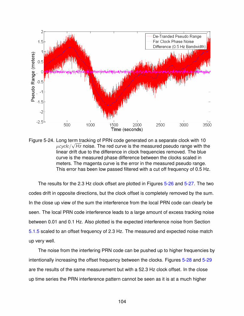
Figure 5-24. Long term tracking of PRN code generated on a separate clock with 10µcycle/
√Hz noise. The red curve is the measured pseudo range with the
linear drift due to the difference in clock frequencies removed. The bluecurve is the measured phase difference between the clocks scaled inmeters. The magenta curve is the error in the measured pseudo range.This error has been low passed filtered with a cut off frequency of 0.5 Hz.
The results for the 2.3 Hz clock offset are plotted in Figures 5-26 and 5-27. The two
codes drift in opposite directions, but the clock offset is completely removed by the sum.
In the close up view of the sum the interference from the local PRN code can clearly be
seen. The local PRN code interference leads to a large amount of excess tracking noise
between 0.01 and 0.1 Hz. Also plotted is the expected interference noise from Section
5.1.5 scaled to an offset frequency of 2.3 Hz. The measured and expected noise match
up very well.
The noise from the interfering PRN code can be pushed up to higher frequencies by
intentionally increasing the offset frequency between the clocks. Figures 5-28 and 5-29
are the results of the same measurement but with a 52.3 Hz clock offset. In the close
up time series the PRN interference pattern cannot be seen as it is at a much higher
104

Figure 5-25. Spectral results of long term tracking of PRN code generated on a separateclock with 10 µcycle/
√Hz noise. At frequencies below 0.02 Hz the DLL
tracks the drift in the incoming code due to the relative phase drift betweenthe clocks. At frequencies above 0.02 Hz the drift between the clocks issmaller than the performance limitation of the DLL.
Figure 5-26. Time series of DLL tracking with interfering code at a clock offset of 2.3 Hz.The sum of the two anti-symmetric measurements removes both the lineardrift and the low frequency fluctuations in due to the relative clock phasenoise. What is left is the noise from the cross correlation between theoutgoing PRN code and the early-late tracking code Section 5.1.5.2).
105

Figure 5-27. Spectral results of DLL tracking with interfering code at clock offset of 2.3Hz. The error in the measured pseudo range is plotted along with theexpected noise contribution from the interfering PRN code. The measuredand expected noise match up very well.
Figure 5-28. Time series of DLL tracking with interfering code at clock offset of 52.3 Hz.The higher difference in clock rates pushes the noise from the interferingcode into higher frequencies.
106
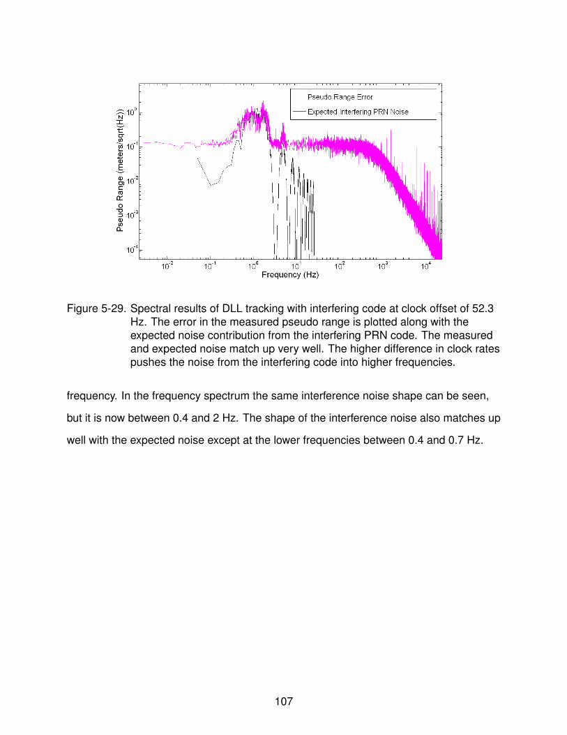
Figure 5-29. Spectral results of DLL tracking with interfering code at clock offset of 52.3Hz. The error in the measured pseudo range is plotted along with theexpected noise contribution from the interfering PRN code. The measuredand expected noise match up very well. The higher difference in clock ratespushes the noise from the interfering code into higher frequencies.
frequency. In the frequency spectrum the same interference noise shape can be seen,
but it is now between 0.4 and 2 Hz. The shape of the interference noise also matches up
well with the expected noise except at the lower frequencies between 0.4 and 0.7 Hz.
107

CHAPTER 6ELECTRONIC TEST OF TDI WITH PRN RANGING
An electronic test of time delay interferometry (TDI) was performed using the
electronic phase delay unit. This test was carried out to determine the ability of the
pseudo-random noise (PRN) code ranging system to accurately measure the delay and
to use this delay to form the TDI X variable (Equation 2–11).
Figure 6-1 is a diagram of the experimental set up. A voltage controlled oscillator
(VCO) and two function generators were used to model the three lasers from each SC
of the LISA constellation. The VCO represents the cavity stabilized laser of the main
SC. It was modulated with PRN code number 1. The other two lasers were modeled
by function generators and were modulated with PRN code number 2. The PRN codes
are applied as a phase modulation, with amplitude 0.14 rad, to a MHz signal that is
generated digitally by a numerically controlled oscillator (NCO). The signal from the
NCO is mixed with the VCO or function generator signal and the resulting signal is split
with one half going through the electronic phase delay (EPD) unit and the other half
being mixed with the signal from the other SC. This experiment used the sample and
hold version of the EPD unit. The EPD unit samples the input signal at 100 MHz; down
samples it to 12.5 MHz, stores it in memory, and then outputs the signal. The travel time
between SC 1 and SC 2 was set to τ3 = 0.5s, and the travel time between SC 1 and SC
3 was set to τ2 = 0.7s. The exact delay in the EPD unit is always roughly a millisecond
longer than the set delay and varies randomly by microseconds from measurement to
measurement. These delays are significantly shorter than the roughly 16s travel times in
the actual LISA mission because the EPD unit is limited in the time it can store data at a
rate of 12.5 MHz.
The simulated sensor signals s21, s31, s12, s13, were measured with the UFLIS
phasemeter. The measured signals contain both a local code and a code that has
been delayed by transmission through the EPD unit (the incoming code). The relative
108

Figure 6-1. Experimental set up of the electronic test of TDI with PRN ranging. A VCO isused to simulate the phase noise of the frequency stabilized master laser,while two function generators simulate the phase-locked slave lasers on theother SC. PRN codes are modulated onto each simulated laser signal andthe sample and hold EPD unit is used to simulate the light travel timebetween SC.
position in time between the local and incoming code was measured for each sensor
signal. The average of this measurement between signals s21 and s12 gives the delay in
arm 3, and the average between signals s31 and s13 gives the delay in arm 2. Both the
tracking of the PRN codes and the measured phase of the sensor signals were recorded
at a rate of 11.9 Hz for 20 hours. Channels 1 and 2 are measured on a separate field
programmable gate array (FPGA) from channels 3 and 4. Hence there is a slight time
delay between the two sets of channels. This time delay was corrected for by adding a
common signal to channels 2 and 4 and measuring the time difference of that common
signal. After the timing correction has been made, the TDI X combination can be formed
as in Equation 2–11. The delays were formed using a 25th order Lagrange filter to
fractionally delay the signals between data points.
109

Figure 6-2. Linear spectral density of the results of the electronic test of TDI with PRNranging. The initial VCO noise level is plotted in red, while the results of theTDI X combination are plotted in magenta. Also plotted is the estimatedlimitation of the TDI X combination due to the noise present in thephasemeter measurement.
The linear spectral density of the results are plotted in Figure 6-2. Also plotted is a
curve of the estimated noise limitation of the phasemeter system. This estimation was
computed by forming the TDI X combination using four independent measurements
of the phasemeter timing jitter (Section 3.6) as the sensor signals. At frequencies less
than the inverse of the round trip delay time of the LISA arms, the response of the
TDI X combination tends to zero as the frequency goes to zero. Since this experiment
had much shorter delay times than the actual LISA mission, the result of the TDI X
combination starts to tend toward zero as the frequency goes below approximately 0.5
Hz.
It was found that the delays used in the TDI X combination could be varied by up to
plus or minus 300 ns before the performance became worse than the measurement
limitation. This corresponds to a ranging accuracy of at worst 10 m. Since the
110
measurement was limited by the performance of the phasemeter system, it is possible
that the performance of the PRN ranging system was actually better.
111
CHAPTER 7FUTURE INTEGRATION OF UFLIS AND LASER COMMUNICATION
The ultimate goal of this work was to integrate the laser communication subsystem
into UFLIS. Chapter 7 describes the first steps taken in order to utilize PRN ranging with
the phasemeter delay unit and to integrate clock transfers into UFLIS.
7.1 PRN Ranging and the Phasemeter Delay Unit
The previously described TDI experiment (Chapter 6) utilized the sample and
hold delay version of the EPD unit because the high data transfer rate of 12.5 MHz
was needed to transfer the high frequency PRN code. The EPD unit is limited in the
maximum length of its delays to 2 seconds and limited in the frequency of the signals
it can delay (up to 6.25 MHz). To overcome these limitations an attempt was made to
modify the phasemeter EPD unit in order to delay PRN codes as well as the phase data.
Figure 7-1 contains a diagram of the modifications to the PM EPD unit. The new delay
unit uses a DLL to track the incoming PRN code. It down samples the position of the
PRN code and sends it through the 4205 model motherboard to the 6228 daughter card
where the PRN code is regenerated. A delay is used to compensate for the added delay
of the CIC filter to the frequency data so that both the frequency data and the PRN code
are delayed by the same time.
Figure 7-1 also contains the experimental set up to measure the performance of the
new EPD unit. The experiment is designed to determine if the new EPD unit preserves
the relative position between the phase noise and the PRN code. The PRN code is
modulated onto a VCO signal by electronic mixing and split with one half sent to the
new EPD unit, delayed for 5 seconds, then sent to the phasemeter, and the other half
sent directly to the phasemeter. At the phasemeter both the phase of the signals and
their pseudo ranges are measured. Fractional delay filtering is used to delay the prompt
signal in post processing and subtract it from the delayed signal. The delay to use in
post processing is found two ways, by searching through a wide range of delays until
112

Figure 7-1. Modifications to the phasemeter EPD unit to include PRN code delays andexperimental set up test the new EPD unit. A DLL loop is used to to track theincoming PRN code. The position of the incoming PRN code is downsampled, stored in memory, and used to regenerate the PRN code. Theexperimental test works by measuring the phase noise and PRN codeposition before and after the EPD unit to determine if the relative position ofthe PRN code and the phase noise is preserved.
the difference between the signals is minimized and by using the measured pseudo
ranges. Figure 7-2 shows that when the minimizing procedure is used the difference
between the two signals reaches the limitation of the phasemeter. The measured
pseudo ranges result in a delay that is roughly 20 micro seconds off from the value
found by minimization. The exact value of this error varies randomly from measurement
to measurement and its cause in unknown.
In its current state the new EPD delay unit cannot be used for TDI. However, there
is no reason to believe that this EPD with PRN concept cannot function properly in
principle. It remains for future work to discover what is limiting the performance of the
new EPD unit and make the necessary modifications.
7.2 Clock Noise Transfers and UFLIS
Intergrating clock noise transfers into the University of Florida LISA Interferometry
Simulator (UFLIS) will require that the sensor signals s21 and s31, s12, and s13 be
113

Figure 7-2. Spectral results of the error in the PRN code timing using the phasemeterEPD unit. The linear spectral density of the VCO noise is plotted in red. Theprompt measurement of the VCO noise is subtracted from the delayedmeasurement using the difference between the prompt and delayed PRNmeasurements (plotted in magenta). Also plotted in green is the difference inthe VCO noise when the delay is found by minimization. Using the PRNdelayed by the EDP leads to a factor of 100 increase in the measurementlimitation.
measured with respect to different clocks. To cancel the clock noise that will appear
in the TDI X variable (Section 2.3.1.3) each of the three numbered lasers (Section 3.2)
will be modulated with their respected clock signals, frequency up-converted to around
2 GHz. In order to electronically delay the GHz sidebands, they must be heterodyned
down to MHz frequencies. This could be accomplished by also modulating the reference
laser with a signal around 2 GHz.
In UFLIS the optical beat notes are simulated by electronic mixers with a laser-reference
laser beat note as one input, representing the local laser, and an electronically delayed
laser-reference laser beat note as the other input, representing the incoming laser.
In the LISA mission the two lasers will each contain a carrier and an upper and lower
114

sideband approximately 2 GHz away from the carrier. Combining these two laser
fields on the photo detector results in three signals, the difference between the lower
sidebands, the carriers, and the upper sidebands.1 In contrast, the electronic mixing of
the prompt and delayed beat notes in UFLIS will result in 18 signals, the difference and
the sum of each cross pair of the six signals.
Figure 7-3 is a diagram of a preliminary test that was carried out to see if the phase
of the three desired signals (the lower sideband-sideband, the carrier-carrier, and the
upper sideband-sideband) could be accurately measured without interference. The
UFLIS optical set up was used to produce two beat notes, one between the two cavity
stabilized lasers (laser 1 and the reference laser), and the other between laser 2 and
the reference laser. Laser 2 was offset phase-locked to the reference laser. Both laser
1 and laser 2 were modulated with a MHz signal. An electronic mixer cannot be used
to mix the two beat notes as they are both modulated (an electronic mixer requires
one un modulated signal used to periodically flip the sign of the other signal). Thus
the multiplication was performed digitally on the FPGA of the digital signal processing
hardware. After the multiplication the resulting signal was sent to three phasemeters
(all on the same FPGA as the multiplier) in order to measure the phase of the lower
sideband-sideband, carrier-carrier, and upper sideband-sideband beat notes. If the
signals have been measured without interference then the combination
CC − 1
2(SSU + SSL) (7–1)
should automatically cancel.
The experiment was repeated many times with several different combinations of
phase lock offsets and modulation frequencies. These frequencies were chosen so
1 The differences between the sidebands and the carrier or between the lower andupper sidebands will be outside the bandwidth of the photo detector.
115

Figure 7-3. Experimental set up of a preliminary test of UFLIS with clock noise transfers.Two beat notes are formed. One with both of the cavity stabilized lasers, L1and RL, and the other with L2 offset phase-locked to RL. Both L1 and L2 arephase modulated with a MHz signal. Both of the photo detector outputs aresampled with the digital signal processing hardware and multiplied digitally.The resulting signal is sent to three phasemeters where the phase of thelower sideband-sideband, carrier-carrier, and upper sideband-sideband beatnotes are measured. The three signals could not be measured withoutinterference.
that the unwanted frequencies resulting from the multiplication would not be within 100
kHz of the three signals to be measured. Nevertheless, forming the combination in
Equation 7–1 always resulted in a significant amount of noise above the phasemeter
measurement limitation.
Thus the clock noise transfers could not be integrated into UFLIS at this time. Since
the cause of the interference is not known, future researchers may be able to discover
its source and correct it.
116

CHAPTER 8CONCLUSION
Gravitational wave astronomy will be an important tool in learning about the
universe, and space based gravitational wave detectors will play an important role in
detecting gravitational waves at low frequencies. This dissertation outlined how the
proposed LISA mission would detect gravitational radiation using laser interferometry.
LISA requires knowledge of the distance between SC to meter accuracy and requires a
method of measuring the relative noise between the separate clocks used to make
interferometric measurements on board each SC. Both of these tasks are to be
accomplished using laser communication subsystems. This dissertation outlined
how these systems will function.
Researchers at the University of Florida have developed a simulator of the LISA
interferometry known as UFLIS. This simulator has been useful in testing several
technologies needed for the success of the LISA mission. This thesis detailed how
UFLIS works and the work that was done to upgrade UFLIS to contain the laser
communication subsystems.
The laser communication subsystems will require both frequency synthesizers
and EOMs in order to transmit clock noise from SC to SC via the laser link. Both
the frequency synthesizers and the EOMs must perform with a phase fidelity of 2 ×
10−4cycles/√Hz at frequencies greater than 3 mHz. The research in this dissertation
demonstrated that the differential noise between two frequency synthesizers was less
than this requirement and that the frequency synthesizers could be used to cancel clock
noise in a phase measurement to the performance limitation of our phasemeter system.
The EOMs were tested at a modulation frequency of 2 GHz and were found to have
a phase fidelity less than the requirement. The frequency synthesizers and the EOMs
were also tested in a differential measurement of their combined phase noise. The
117

differential phase noise of the frequency synthesizer and EOM combination was found to
be lower than the requirement.
This dissertation also described in detail the design of a DLL to track the changing
distances between SC. In the course of designing the DLL it was discovered that the
double frequency term that arises from the multiplication of the received beat note with
the local oscillator inside the phasemeter, introduces noise in the error signal formed by
the DLL. This noise was greatest for beat notes at frequencies less than 3 MHz. A time
domain filter was designed to reproduce the double frequency term and subtract it out
of the signal before the DLL. This filter was able to attenuate the double frequency term
by a factor of 20, resulting in a significant improvement in the error signals formed by the
DLL.
The design of the DLL was described in detail as well as the limitation of its
performance due to the shot noise present at the photodetector and the interference
from the outgoing PRN code. The DLL was tested in simulation as well as with LISA-like
hardware including lasers, EOMs, photo detectors, and the UFLIS phasemeter.
Several experiments were performed culminating in a measurement that included a
10µcycle/√Hz noise level and interfering PRN codes running on independent clocks.
Both the simulation and this measurement were able to verify that the PRN ranging
scheme meets the 1 meter root mean square error requirement at a measurement
bandwidth of 0.5 Hz. The experiments also demonstrated that the noise from the
interfering PRN code can be shifted to higher frequencies by intentionally increasing the
frequency difference between clocks on separate SC.
The PRN ranging scheme was also tested in an electronic TDI experiment using
the sample and hold EPD unit. This experiment showed that the values of the delay
times obtained by PRN ranging were suitable to use in forming the TDI X combination.
The VCO noise (simulating laser noise) was suppressed by the TDI combination to the
118

performance limit of the phasemeter. It was shown that the PRN ranging measurement
was accurate to at worst 10 meters.
Finally this dissertation outlined the initial work that was done in integrating the
laser communications subsystems into UFLIS. Two limiting problems were identified
which must be solved by future researchers in order to successfully integrate the laser
communications subsystems into UFLIS.
119
REFERENCES
[1] J. Taylor and J. Weisberg. A new test of general relativity: gravitational radiationand the binary pulsar psr 1913+16. Astrophy. J., 253, 1982.
[2] B. F. Shutz. Determining the hubble constant from gravitational wave observations.Nature, 323, 1986.
[3] B. R. Iyer L. Blanchet, G. Faye and B. Joguet. Gravitational-wave inspiral ofcompact binary systems to 7/2 post-newtonian order. Phys. Rev. D, 65, 2002.
[4] D. I. Choi M. Koppitz J. G. Baker, J. Centrella and J. van Meter. Binary black holemerger dynamics and waveforms. Phys. Rev. D, 73, 2006.
[5] B. J. Owen and B. S. Sathyaprakash. Matched filtering of gravitational waves frominspiraling compact binaries: Computational cost and template placement. Phys.Rev. D, 60, 1999.
[6] S. Nissanke I. MacDonald and H. P. Pfeiffer. Suitability ofpost-newtonian/numerical-relativity hybrid waveforms for gravitational wavedetectors. Class. Quantum Grav., 28, 2011.
[7] N. A. Collins and S. A. Hughes. Towards a formalism for mapping the spacetimesof massive compact objects: Bumpy black holes and their orbits. Phys. Rev. D, 69,2004.
[8] F. D. Ryan. Gravitational waves from the inspiral of a compact object into amassive, axisymmetric body with arbitrary multipole moments. Phys. Rev. D, 52,1995.
[9] M. Shibata. Axisymmetric general relativistic hydrodynamics: Long-term evolutionof neutron stars and stellar collapse to neutron stars and black holes. Phys. Rev. D,67, 2003.
[10] H. T. Janka K. Kifonidis L. Scheck, T. Plewa and E. Mueller. Pulsar recoil bylarge-scale anisotropies in supernova explosions. Phys. Rev. Lett., 92, 2004.
[11] H.Th. Janka E. Mller and A. Wongwathanarat. Parametrized 3d models ofneutrino-driven supernova explosions. A and A, 537, 2012.
[12] N. Andersson. A new class of unstable modes of rotating relativistic stars. Astro-phys. J., 502, 1998.
[13] B. J. Owen L. Lindblom and S. M. Morsink. Gravitational radiation instability in hotyoung neutron stars. Phys. Rev. Lett., 80, 1998.
[14] C. Cutler B. F. Schutz A. Vecchio B. J. Owen, L. Lindblom and N. Andersson.Gravitational waves from hot young rapidly rotating neutron stars. Phys. Rev. D, 58,1998.
120

[15] L. Bildsten. Gravitational radiation and rotation of accreting neutron stars. Astro-phys. J., 501, 1998.
[16] D. Jones. Gravitational waves from rotating strained neutron stars. ClassicalQuantum Gravity, 19, 2002.
[17] S. Dodelson L. M. Krauss and S. Meyer. Primordial gravitational waves andcosmology. Science, 328, 2010.
[18] P.Astone et al. Results of the igec-2 search for gravitational wave bursts during2005. Phys. Rev. D, 76, 2007.
[19] P.Astone et al. Methods and results of the igec search for burst gravitational wavesin the years1997-2000. Phys. Rev. D, 68, 2003.
[20] F. Acernese et al. First joint gravitational wave search by theaurigaexplorernautilusvirgo collaboration. Class. Quantum Grav., 25, 2008.
[21] L. Baggio et al. A joint search for gravitational wave bursts with auriga and ligo.Class. Quant. Grav., 25, 2008.
[22] P.Astone et al. Upper limit for a gravitational-wave stochastic background with theexplorer and nautilus resonant detectors. Phys. Letters B, 385, 1996.
[23] J. P. W. Verbiest et al. Precision timing of psr j04374715: An accurate pulsardistance, a high pulsar mass, and a limit on the variation of newton’s gravitationalconstant. Astrophys. J., 679, 2008.
[24] F. A. Jenet et al. Constraining the properties of supermassive black hole systemsusing pulsar timing: Application to 3c 66b. Astrophys. J., 606, 2004.
[25] A. Vecchio A. Sesana and C. N. Colacino. The stochastic gravitational-wavebackground from massive black hole binary systems: implications for observationswith pulsar timing arrays. Mon. Not. R. Astron. Soc., 390, 2008.
[26] Ryutaro Takahashi and the TAMA Collaboration. Status of tama300. Class.Quantum Grav., 21, 2004.
[27] B. Abbott et al. Upper limits from the ligo and tama detectors on the rate ofgravitational-wave bursts. Phys. Rev. D, 72, 2005.
[28] G. Ballardin et al. Measurement of the virgo superattenuator performance forseismic noise suppression. Rev. Sci. Instrum., 72, 2001.
[29] B. P. Abbott et al. Search for gravitational waves from low mass binarycoalescences in the first year of ligos s5 data. Phys. Rev. Lett., 79, 2009.
[30] B. P. Abbott et al. All-sky ligo search for periodic gravitational waves in the earlyfifth-science-run data. Phys. Rev. Lett., 102, 2009.
121

[31] B. P. Abbott et al. Stacked search for gravitational waves from the 2006 sgr1900+14 storm. Astrophys. J., 701, 2009.
[32] J Abadie et al. Predictions for the rates of compact binary coalescences observableby ground-based gravitational-wave detectors. Class. Quantum Grav., 27, 2010.
[33] W. M. Folkner et al. Lisa orbit selection and stability. Class. Quantum Grav., 14,1997.
[34] Z. Silvestri et al. Volume magnetic susceptibility of goldplatinum alloys: possiblematerials to make mass standards for the watt balance experiment. Metrologia, 40,2003.
[35] E. J. Elliffe et al. Hydroxide-catalysis bonding for stable optical systems for space.Class. Quantum Grav., 22, 2005.
[36] P. Bender, K. Danzmann, and the LISA Study Team. Laser Interferometer SpaceAntenna for the Detection and Observation of Gravitational Waves Pre-Phase AReport. Max-Planck-Institut fur Quantenoptik, Garching, 2nd edition, 1998.
[37] Rachel J. Cruz. Development of the UF LISA Benchtop Simulator for Time DelayInterferometry. PhD thesis, University of Florida, 2006.
[38] Alix Preston. Stability of materials for use in space-based interferometric missions.PhD thesis, University of Florida, 2010.
[39] V. Leonhardt and J. B. Camp. Space interferometry application of laser frequencystabilization with molecular iodine. Applied Optics, 45, 2006.
[40] V. Wand et al. Noise sources in the ltp heterodyne interferometer. Class. QuantumGrav., 23, 2006.
[41] A. F. Garca Marn et al. Phase locking to a lisa arm: first results on a hardwaremodel. Class. Quantum Grav., 22, 2005.
[42] James Ira Thorpe. Laboratory Studies of Arm-Locking Using the Laser Interferom-etry Space Antenna Simulator at the University of Florida. PhD thesis, University ofFlorida, 2006.
[43] Yinan Yu. Arm Locking for Laser Interferometer Space Antenna. PhD thesis,University of Florida, 2011.
[44] Massimo Tinto, Daniel A. Shaddock, Julien Sylvestre, and J. W. Armstrong.Implementation of time-delay interferometry for lisa. Phys. Rev. D, 67(12), 2003.
[45] D. A. Shaddock, B.Ware, R. E. Spero, and M. Vallisneri. Postprocessed time-delayinterferometry for lisa. Phys. Rev. D, 70(8), 2004.
[46] F. B. Estabrook M. Tinto and J. W. Armstrong. Time delay interferometry withmoving spacecraft arrays. Phys. Rev. D, 69, 2004.
122
[47] T. Prince et al. Lisa: Unveiling a hidden universe: Assessment study report.European Space Agency documentation, 2011.
[48] Juan Jose Esteban, Iouri Bykov, Antonio Francisco, Gerhard Heinzel Garcia Marin,and Karsten Danzmann. Optical ranging and data transfer development for lisa.Journal of Physics: Conference Series, 154, 2009.
[49] Massimo Tinto, Michele Vallisneri, and J.W. Armstrong. Time-delay interferometricranging for space-borne gravitational-wave detectors. Phys. Rev. D, 71, 2005.
[50] V. Wand S. Mitryk and G. Mueller. Verification of time-delay interferometrytechniques using the university of florida lisa interferometry simulator. Class.Quantum Grav., 27, 2010.
[51] S. Mitryk Y. Yu and G. Mueller. Experimental validation of dual/modified dual armlocking for lisa. Class. Quantum Grav., 28, 2011.
[52] Shawn Mitryk. Laser noise mitigation through time delay interferometry forspace-based gravitational wave interferometers using the UF laser interferometrysimulator. PhD thesis, University of Florida, 2012.
[53] E. Black. An introduction to pound drever hall laser frequency stabilization. Am. J.Phys., 69, 2001.
[54] Shaddock D. et. al.. Lisa frequency control white paper. Technical report, TheFrequency Control Study Team, 2009.
[55] R. J. Cruz et. al. The lisa benchtop simulator at the university of florida. Class.Quantum Grav., .
[56] J. I. Thorpe and G. Mueller. Experimental verification of arm-locking for lisa usingelectronic phase delay. Phys. Lett. A, 342, 2005.
[57] V. Wand et. al. Implementation of armlocking with a delay of 1 second in thepresence of doppler shifts. J. Phys.: Conf. Ser., .
[58] S. Mitryk Y. Yu, V. Wand and G. Mueller. Arm locking with doppler estimation errors.J. Phys. Conf. Ser., 228, 2010.
[59] S. Mitryk and G. Mueller. Demonstration of time delay interferometry andspacecraft ranging in a space-based gravitational wave detector using the uf-lisainterferometry simulator. In Publication, 2012.
[60] A. Sutton et. al. Laser ranging and communications for lisa. Optics Express, .
[61] R. E. Ziemer. Fundamentals of Spread Spectrum Modulation. Morgan andClaypool, 2007.
[62] R. E. Ziemer and R. L. Peterson. Digital Communications and Spread SpectrumSystems. Macmillan Publishing Company, 1985.
123

BIOGRAPHICAL SKETCH
Dylan Sweeney was raised by a wonderful and loving family in Tacoma Washington.
He attended the University of Hawai‘i at Manoa where he graduated with a Bachelor of
Science in physics in 2006. He attended graduate school at the University of Florida
where he joined the Laser Interferometer Space Antenna (LISA) group under Dr. Mueller
in 2007. He met his wife, Sandra Londono, in 2007 at the University of Florida and
married her in 2009. They had their first child, Nicolas Sweeney, in 2011.
124