las & x-las - campbell sci appendix i – theory scintillation technique 41 appendix ii –...
TRANSCRIPT
Instruction Manual
(Extra) Large Aperture ScintillometerLAS & X-LAS

WARRANTY AND ASSISTANCE This equipment is warranted by CAMPBELL SCIENTIFIC (CANADA) CORP. (“CSC”) to be free from defects in materials and workmanship under normal use and service for twelve (12) months from date of shipment unless specified otherwise. ***** Batteries
are not warranted. ***** CSC's obligation under this warranty is limited to repairing or replacing (at CSC's option) defective products. The customer shall assume all costs of removing, reinstalling, and shipping defective products to CSC. CSC will return such products by surface carrier prepaid. This warranty shall not apply to any CSC products which have been subjected to modification, misuse, neglect, accidents of nature, or shipping damage. This warranty is in lieu of all other warranties, expressed or implied, including warranties of merchantability or fitness for a particular purpose. CSC is not liable for special, indirect, incidental, or consequential damages. Products may not be returned without prior authorization. To obtain a Return Merchandise Authorization (RMA), contact CAMPBELL SCIENTIFIC (CANADA) CORP., at (780) 454-2505. An RMA number will be issued in order to facilitate Repair Personnel in identifying an instrument upon arrival. Please write this number clearly on the outside of the shipping container. Include description of symptoms and all pertinent details. CAMPBELL SCIENTIFIC (CANADA) CORP. does not accept collect calls. Non-warranty products returned for repair should be accompanied by a purchase order to cover repair costs.
1
IMPORTANT USER INFORMATION
Reading this entire manual is essential for full understanding of the proper use and safe operation of this product
Should you have any comments on this manual we will be pleased to receive them at:
Kipp & Zonen B.V. Delftechpark 36 2628 XH Delft Holland P.O. Box 507 2600 AM Delft Holland Phone +31 (0)15 275 5210 Fax +31 (0)15 262 0351 Email [email protected]
Kipp & Zonen reserves the right to make changes to the specifications without prior notice.
WARRANTY AND LIABILITY
Kipp & Zonen guarantees that the product delivered has been thoroughly tested to ensure that it meets its published specifications. The warranty included in the conditions of delivery is valid only if the product has been installed and used according to the instructions supplied by Kipp & Zonen. Kipp & Zonen shall in no event be liable for incidental or consequential damages, including without limitation, lost profits, loss of income, loss of business opportunities, loss of use and other related exposures, however caused, arising from the faulty and incorrect use of the product. User made modifications can affect the validity of the CE declaration.
COPYRIGHT© 2007 KIPP & ZONEN
All rights reserved. No part of this publication may be reproduced, stored in a retrieval system or transmitted in any form or by any means, without permission in written form from the company. Manual version: 0307

2
Throughout the manual symbols are used to indicate to the user important information. The meaning of these symbols is as follows:
The exclamation mark within an equilateral triangle is intended to alert the user to the presence of important operating, maintenance and safety information
3
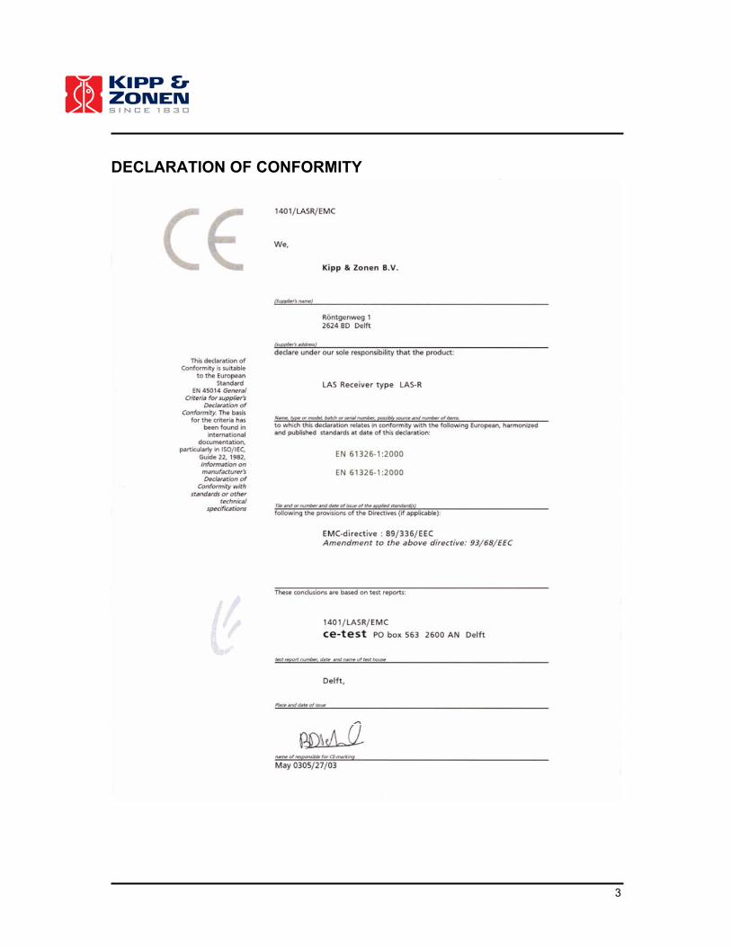
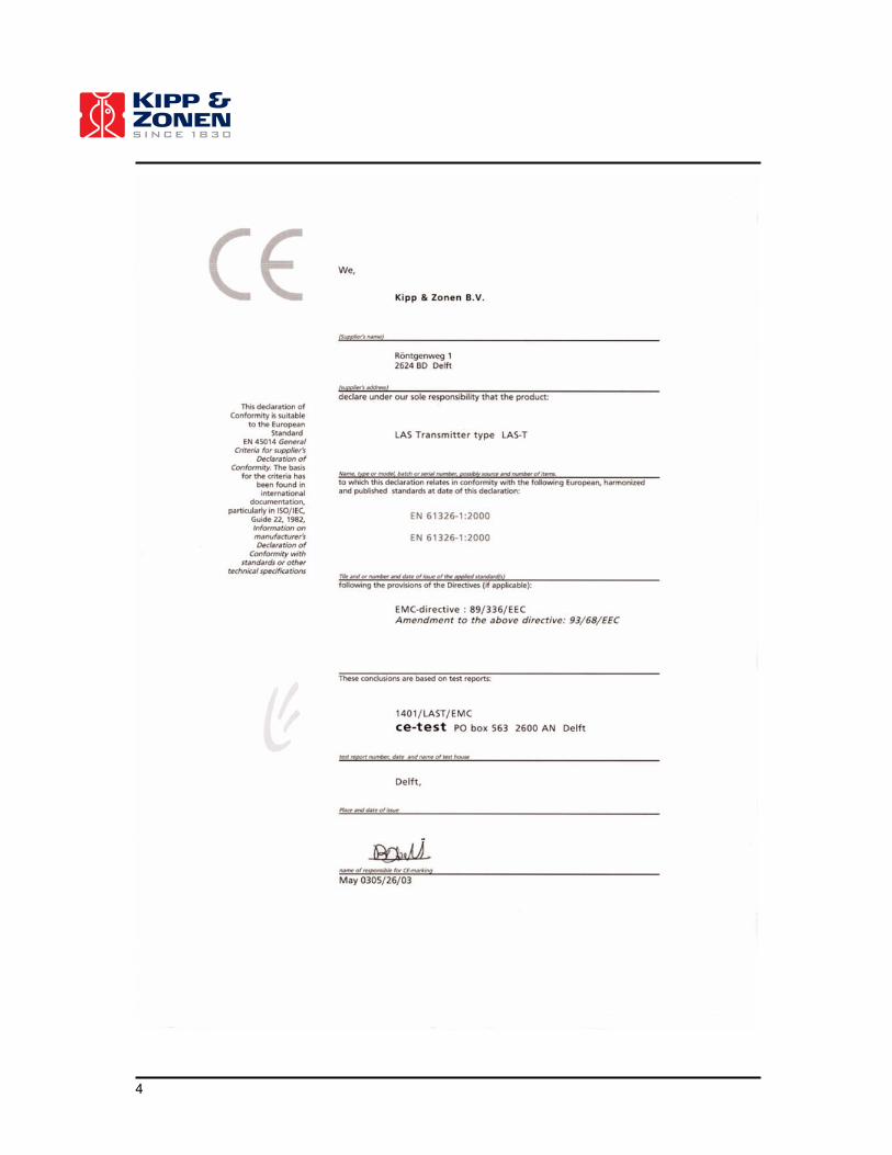
DECLARATION OF CONFORMITY
4
5
TABLE OF CONTENTS
IMPORTANT USER INFORMATION.......................................................................................1 WARRANTY AND LIABILITY .............................................................................................................. 1 COPYRIGHT© 2007 KIPP & ZONEN .................................................................................................. 1
DECLARATION OF CONFORMITY ........................................................................................3
TABLE OF CONTENTS...........................................................................................................5
LIST OF SYMBOLS AND ABBREVIATIONS .........................................................................7 SYMBOLS............................................................................................................................................ 7 ABBREVIATIONS................................................................................................................................ 8
1. GENERAL INFORMATION .................................................................................................9 1.1 INTRODUCTION TO THE LAS AND XLAS .................................................................................. 9 1.2 MANUAL ...................................................................................................................................... 10
2. TECHNICAL DATA............................................................................................................11
3. INSTALLATION.................................................................................................................13 3.1 DELIVERY ................................................................................................................................... 13 3.2 ORIENTATION PATH / SITE SELECTION ................................................................................. 14 3.3 HEIGHT – PATH LENGTH .......................................................................................................... 14
3.3.1 Minimum height – Saturation ................................................................................................ 14 3.3.2 Minimum and maximum height – MOST............................................................................... 16
3.4 THE MOUNTING SUPPORT....................................................................................................... 17 3.5 MOUNTING THE LAS AND XLAS .............................................................................................. 17 3.6 ELECTRICAL CONNECTION ..................................................................................................... 17
3.6.1 Amphenol socket................................................................................................................... 17 3.6.2 BNC socket ........................................................................................................................... 18 3.6.3 Protection circuitry and fuse ratings...................................................................................... 19
3.7 OPTICAL ALIGNMENT ............................................................................................................... 20 3.8 SETTING PATH LENGTH POTENTIOMETER........................................................................... 24
4. OPERATION......................................................................................................................27
5. WINLAS SOFTWARE........................................................................................................29 5.1 SYSTEM REQUIREMENTS ........................................................................................................ 29 5.2 INSTALLATION ........................................................................................................................... 29 5.3 WINLAS OVERVIEW................................................................................................................... 29 5.4 THE INPUT FILE ......................................................................................................................... 31 5.5 THE OUTPUT FILE ..................................................................................................................... 33
6. MAINTENANCE.................................................................................................................35
7. CALIBRATION...................................................................................................................37 7.1 ON-SITE CALIBRATION CHECK................................................................................................ 37 7.2 RECALIBRATION........................................................................................................................ 38 7.3 CALIBRATION PROCEDURE AT KIPP & ZONEN..................................................................... 38
7.3.1 Calibration procedure RMS-circuits ...................................................................................... 38 7.3.2 Calibration path length .......................................................................................................... 38
8. SOLVING PROBLEMS......................................................................................................39 8.1 PROBLEM CHECK-LIST............................................................................................................. 39 8.2 TROUBLESHOOTING................................................................................................................. 39
6
APPENDIX I – THEORY SCINTILLATION TECHNIQUE .....................................................41
APPENDIX II – PATH-WEIGHTING FUNCTION LAS/XLAS................................................49
APPENDIX III – ROUGHNESS LENGTH & DISPLACEMENT HEIGHT ..............................51
APPENDIX IV – HEATER AND THERMISTOR ....................................................................53
APPENIDX V – CR10X CAMPBELL PROGRAM .................................................................55
APPENDIX VI – COMBILOG PROGRAM .............................................................................59
APPENDIX VII – DIAPHRAGMS FOR SHORT RANGE APPLICATIONS ...........................63
APPENDIX VIII – RECALIBRATION SERVICE ....................................................................67
7
LIST OF SYMBOLS AND ABBREVIATIONS
SYMBOLS
AT wavelength dependant constants [-] AQ wavelength dependant constants [-] cp heat capacity of air at constant pressure [�1005 J kg-1 K-1]
Cn2 structure parameter of the refractive index of air [m-2/3] (
� �122 210�� CNU
nC )
CT2 structure parameter of temperature [K2 m-2/3]
CQ2 structure parameter of humidity [kg2 m-6 m-2/3]
d zero-displacement height [m] D aperture diameter of receiver and transmitter unit [m] fT universal stability function [-] g gravitational acceleration [�9.81 m s-2] Gs soil heat flux [W m-2] H sensible heat flux [W m-2] I signal strength or intensity [V] (I = UDEMOD) L path length [m] LvE latent heat flux (or evaporation) [W m-2] LMO Obukhov length [m] Pot potentiometer path length setting at Path length knob [-] P air pressure [Pa] PUCN2 scaled Cn
2 [m-2/3] (Cn2 = PUCN2�10-15)
Q absolute humidity [kg m-3] Q* net radiation [W m-2] Rd specific gas constant for dry air [�287 J K-1 kg-1] Rv specific gas constant for water vapour [�461.5 J K-1 kg-1] T absolute air temperature [K] T* temperature scale [K] u wind speed [m s-1] u* friction velocity [m s-1]
UCN2 log Cn2 signal [V] (
� �122 210�� CNU
nC ) [-5 V to 0 V]
UDEMOD demodulated signal [V] (UDEMOD = I) [-1 V to 0 V] UTH_R thermistor signal receiver unit [V] [0 V to 10 V] UTH_T thermistor signal transmitter unit [V] [0 V to 10 V)] zLAS (effective) height LAS or XLAS [m] z0 aerodynamic roughness length [m] zu height wind speed measurements [m] � Bowen ratio [-] (� = H/LvE) v von Kármán constant (�0.40) wavelength of EM radiation (880 nm) [m] � density of air [kg m-3] [�1.2 kg m-3 (at sea level !)]
2� variance
2
ln I� of natural logarithm of intensity fluctuations ( ln(I) ) [-]
22
IUDEMOD�� � of UDEMOD or intensity I [V2]
2
2CNU� of UCN2 [V2]
m integrated stability function for momentum [-]
8
ABBREVIATIONS
(X)LAS (eXtra) Large Aperture Scintillometer MOST Monin-Obukhov Similarity Theory
A relationship describing the vertical behavior of non-dimensionalized mean flow and turbulence properties within the Surface Layer as a function of the Monin–Obukhov key parameters.
PBL Planetary Boundary Layer The PBL is the lowest region of the troposphere, which is directly affected by heating and cooling of the earth surface. In general the depth of the PBL varies between 100m to 2000m. The depth of the PBL increases during the day, when the surface is heated by the sun and decreases during the night.
RS Roughness Sublayer Lowest part of the SL, where the flow is influenced by individual roughness elements. Consequently, the SL can be divided into the Constant Flux Layer and the Roughness Sublayer. The height of the Roughness Sublayer strongly depends on the height (size and form) of the roughness elements, but also on the distribution. Usually, over tall vegetation 3 times the obstacle height is taken as the height of the Roughness Sublayer.
SL Surface Layer In general in the lowest 10% of the PBL the surface fluxes are constant with height, this part of the PBL is also known as the Constant Flux Layer of Surface Layer (SL). Therefore fluxes measured in the SL can be considered as being representative fluxes for the heat and mass exchange processes between the atmosphere and the surface. In general the SL begins at 3 times the vegetation height and has a typical depth of 20m (at night) to 100m (during daytime conditions).

9
1. GENERAL INFORMATION
1.1 INTRODUCTION TO THE LAS AND XLAS
The Large Aperture Scintillometer (LAS) and eXtra Large Aperture Scintillometer (XLAS) are instruments designed for measuring the path-averaged structure parameter of the refractive index of air (Cn
2) over horizontal path lengths from 250 m to 4.5 km1 (LAS) and 1 km to 8 km1 (XLAS). Structure parameter measurements obtained with the LAS or XLAS and standard meteorological observations (air temperature, wind speed and air pressure) can be used to derive the surface sensible heat flux (H). The LAS and XLAS optically measure intensity fluctuations (known as scintillations) using a transmitter and receiver horizontally separated by several kilometers. The scintillations seen by the instrument can be expressed as the structure parameter of the refractive index of air (Cn
2). The light source of the LAS and XLAS transmitter operates at a near-infrared wavelength of 880 nm. At this wavelength the observed scintillations are primarily caused by turbulent temperature fluctuations. Therefore Cn
2 measurements obtained with the LAS or XLAS can be related the sensible heat flux. Compared to traditional point measurements the LAS and XLAS operate at spatial scales comparable to the grid box size of numerical models and pixels of satellite images used in meteorology, hydrology and water-management studies. The LAS and XLAS have important applications in energy balance and also water balance studies, because the surface flux of sensible heat is linked to evaporation (LvE). Some key LAS and XLAS features are:
� Heated transmitter and receiver windows and internal temperature monitoring provide a mechanism to eliminate condensation problems.
� Simple construction using Fresnel lenses for collimation and collection of the light permits path
lengths up to 4.5 km (LAS) and 8 km (XLAS) (depending on atmospheric conditions). Unlike mirror-based scintillometers the Fresnel lens avoids obstruction of the beam by the transmitting LED or the receiving detector.
� On-board calibration and reference signals at the receiver electronics allow rapid on-site
confirmation of operation. Either the received carrier signal or the reference waveform can be monitored on the rear panel BNC output.
� Surge, over-voltage and lightning protection for both the transmitter and receiver units are
standard.
� Eye-safe near-infrared light source.
� 12 Volt DC power for flexibility of use.
� Built-in pan and tilt adjuster for easier alignment.
1 Depending on atmospheric conditions
10
1.2 MANUAL
The INSTRUCTION MANUAL is intended for customers who have purchased the LAS or XLAS. It includes all the information necessary to properly install and operate the LAS/XLAS and how to derive the sensible heat flux from the LAS/XLAS measurements. An appendix (appendix I) is added to the manual for users who are interested in the theoretical background on scintillometry and the derivation of the surface sensible heat flux (see also WINLAS help file) and references to scientific papers.
11
2. TECHNICAL DATA
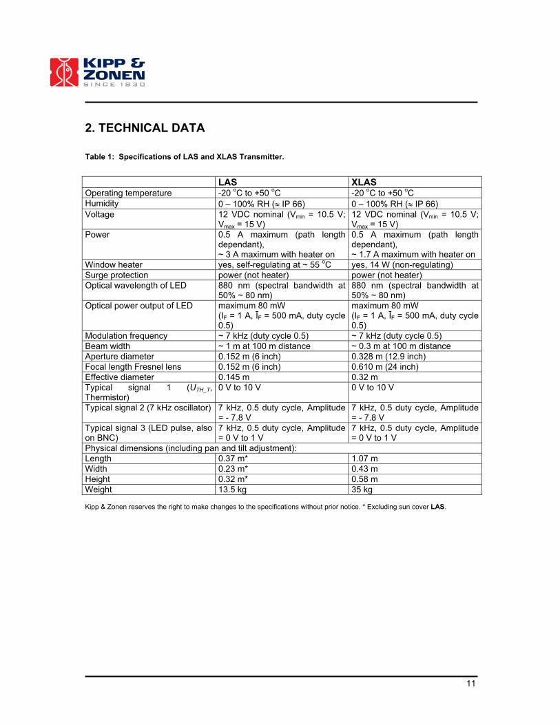
Table 1: Specifications of LAS and XLAS Transmitter.
LAS XLAS Operating temperature -20 oC to +50 oC -20 oC to +50 oC Humidity 0 – 100% RH (� IP 66) 0 – 100% RH (� IP 66) Voltage 12 VDC nominal (Vmin = 10.5 V;
Vmax = 15 V) 12 VDC nominal (Vmin = 10.5 V; Vmax = 15 V)
Power 0.5 A maximum (path length dependant), ~ 3 A maximum with heater on
0.5 A maximum (path length dependant), ~ 1.7 A maximum with heater on
Window heater yes, self-regulating at ~ 55 oC yes, 14 W (non-regulating) Surge protection power (not heater) power (not heater) Optical wavelength of LED 880 nm (spectral bandwidth at
50% ~ 80 nm) 880 nm (spectral bandwidth at 50% ~ 80 nm)
Optical power output of LED maximum 80 mW (IF = 1 A, �F = 500 mA, duty cycle 0.5)
maximum 80 mW (IF = 1 A, �F = 500 mA, duty cycle 0.5)
Modulation frequency ~ 7 kHz (duty cycle 0.5) ~ 7 kHz (duty cycle 0.5) Beam width ~ 1 m at 100 m distance ~ 0.3 m at 100 m distance Aperture diameter 0.152 m (6 inch) 0.328 m (12.9 inch) Focal length Fresnel lens 0.152 m (6 inch) 0.610 m (24 inch) Effective diameter 0.145 m 0.32 m Typical signal 1 (UTH_T, Thermistor)
0 V to 10 V 0 V to 10 V
Typical signal 2 (7 kHz oscillator) 7 kHz, 0.5 duty cycle, Amplitude = - 7.8 V
7 kHz, 0.5 duty cycle, Amplitude = - 7.8 V
Typical signal 3 (LED pulse, also on BNC)
7 kHz, 0.5 duty cycle, Amplitude = 0 V to 1 V
7 kHz, 0.5 duty cycle, Amplitude = 0 V to 1 V
Physical dimensions (including pan and tilt adjustment): Length 0.37 m* 1.07 m Width 0.23 m* 0.43 m Height 0.32 m* 0.58 m Weight 13.5 kg 35 kg Kipp & Zonen reserves the right to make changes to the specifications without prior notice. * Excluding sun cover LAS.
12
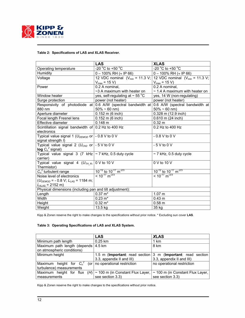
Table 2: Specifications of LAS and XLAS Receiver.
LAS XLAS Operating temperature -20 oC to +50 oC -20 oC to +50 oC Humidity 0 – 100% RH (� IP 66) 0 – 100% RH (� IP 66) Voltage 12 VDC nominal (Vmin = 11.3 V;
Vmax = 15 V) 12 VDC nominal (Vmin = 11.3 V; Vmax = 15 V)
Power 0.2 A nominal, ~3 A maximum with heater on
0.2 A nominal, ~ 1.4 A maximum with heater on
Window heater yes, self-regulating at ~ 55 oC yes, 14 W (non-regulating) Surge protection power (not heater) power (not heater) Responsivity of photodiode at 880 nm
0.6 A/W (spectral bandwidth at 50% ~ 60 nm)
0.6 A/W (spectral bandwidth at 50% ~ 60 nm)
Aperture diameter 0.152 m (6 inch) 0.328 m (12.9 inch) Focal length Fresnel lens 0.152 m (6 inch) 0.610 m (24 inch) Effective diameter 0.148 m 0.32 m Scintillation signal bandwidth of electronics
0.2 Hz to 400 Hz 0.2 Hz to 400 Hz
Typical value signal 1 (UDEMOD or signal strength I)
- 0.8 V to 0 V - 0.8 V to 0 V
Typical value signal 2 (UCN2 or log Cn
2 signal) - 5 V to 0 V - 5 V to 0 V
Typical value signal 3 (7 kHz carrier)
~ 7 kHz, 0.5 duty cycle ~ 7 kHz, 0.5 duty cycle
Typical value signal 4 (UTH_R, Thermistor)
0 V to 10 V 0 V to 10 V
Cn2 turbulent range 10-12 to 10-17 m-2/3 10-12 to 10-17 m-2/3
Noise level of electronics (UDEMOD = - 0.8 V; LLAS = 1184 m; LXLAS = 2152 m)
< 10-17 m-2/3 < 10-17 m-2/3
Physical dimensions (including pan and tilt adjustment): Length 0.37 m* 1.07 m Width 0.23 m* 0.43 m Height 0.32 m* 0.58 m Weight 13.5 kg 35 kg Kipp & Zonen reserve the right to make changes to the specifications without prior notice. * Excluding sun cover LAS.
Table 3: Operating Specifications of LAS and XLAS System.
LAS XLAS Minimum path length 0.25 km 1 km Maximum path length (depends on atmospheric conditions)
4.5 km 8 km
Minimum height 1.5 m (Important: read section 3.3, appendix II and III)
3 m (Important: read section 3.3, appendix II and III)
Maximum height for Cn2 (or
turbulence) measurements no operational restriction no operational restriction
Maximum height for flux (H) measurements
~ 100 m (in Constant Flux Layer, see section 3.3)
~ 100 m (in Constant Flux Layer, see section 3.3)
Kipp & Zonen reserve the right to make changes to the specifications without prior notice.
13
3. INSTALLATION The following steps must be carefully taken for optimal performance of the instrument.
3.1 DELIVERY
Check the contents of the shipment for completeness (see below) and note whether any damage has occurred during transport. If there is damage, a claim should be filed with the carrier immediately. In this case, or if the contents are incomplete, the Kipp & Zonen Sales or Services organization should be notified in order to facilitate the repair or replacement of the instrument. The LAS/XLAS scintillometer delivery will include the following items:
� (X)LAS transmitter (with pan and tilt adjuster) � (X)LAS receiver (with pan and tilt adjuster) � 2 � sun / weather cover � 2 � sighting telescope with detachable mountings � 2 � 0.1m diaphragms to adjust the LAS for short range applications (plus add. screws,
washers and spacers) � 2 � 5 m cable with 10 lead, fitted with a 10-way circular amphenol plug (male) at one end � 4 spare bags of silica gel (5 gr. each) � A CD containing WINLAS and a pdf-file of the LAS/XLAS manual
Any missing parts should be reported to your dealer, who will suggest appropriate action. Unpacking Keep the original packaging for later shipments! Although the LAS/XLAS is weatherproof and suitable for rough ambient conditions, the transmitter and receiver do contain delicate optical and electronic parts. For this type of equipment, keep the original shipment packaging to safely transport the equipment to the measurement sites.
14
3.2 ORIENTATION PATH / SITE SELECTION
Avoid direct sunlight in both the receiver and transmitter windows to prevent overheating of the LED and permanent damage to the detector. It is recommended to select a path that is approximately parallel to the earth’s surface (i.e. horizontal) and has a north-south orientation to avoid problems caused by low sun angles.
Important: Exposure to direct sunlight can permanently damage the optical parts (LED and detector).
Important: Verify that the optical path of the LAS or XLAS is always free from obstacles (e.g. trees, buildings).
3.3 HEIGHT – PATH LENGTH
To be certain that the Cn
2 measurements of the LAS/XLAS are reliable and fluxes (of sensible heat H and latent heat LvE) can be derived from these measurements it is very important to follow the instructions/recommendations given in the following two sections.
3.3.1 Minimum height – Saturation
When the scintillation intensity rises above a certain limit the theory, on which the scintillation measurement method is based, is no longer valid. When this occurs the relationship between the measured amount of scintillations (�lnI
2) and the structure parameter of the refractive index of air (Cn2)
fails. This phenomenon is known as saturation. In order to prevent saturation, Cn2 must stay below a
certain saturation criterion (Smax), i.e. the scintillometer can operate only under weakly scintillating conditions. The dependence of Cn
2 on the optical wavelength (), the aperture diameter (D), the measurement height (zLAS) and the path length (L) can be written as follows
max
2 ),,,( SLzDC LASn � .
The path length and the measurement height are the only variables that can be adjusted in order to keep Cn
2 below the saturation criterion because the diameter and the wavelength of the LAS and XLAS are constant. A scintillometer installed at a height close the earth’s surface, will see more scintillations than a scintillometer installed high above the surface. As the path length increases more scintillations will be observed. This means that over long distances (~ several kilometres) the scintillometer must be placed high above the surface in order to prevent saturation. Over short distances (~ several hundred meters) the scintillometer can be installed close to the surface. Furthermore, the measured amount of scintillations depends on the surface conditions. Over dry areas the surface sensible heat flux is large, resulting in higher Cn
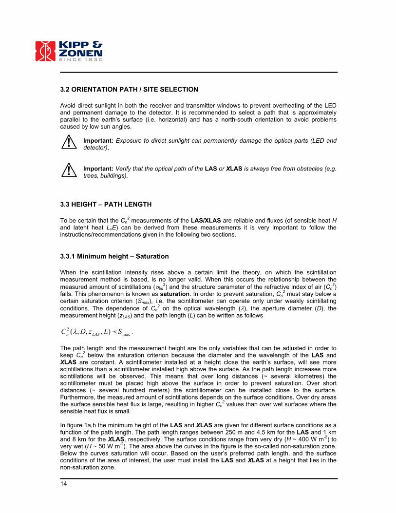
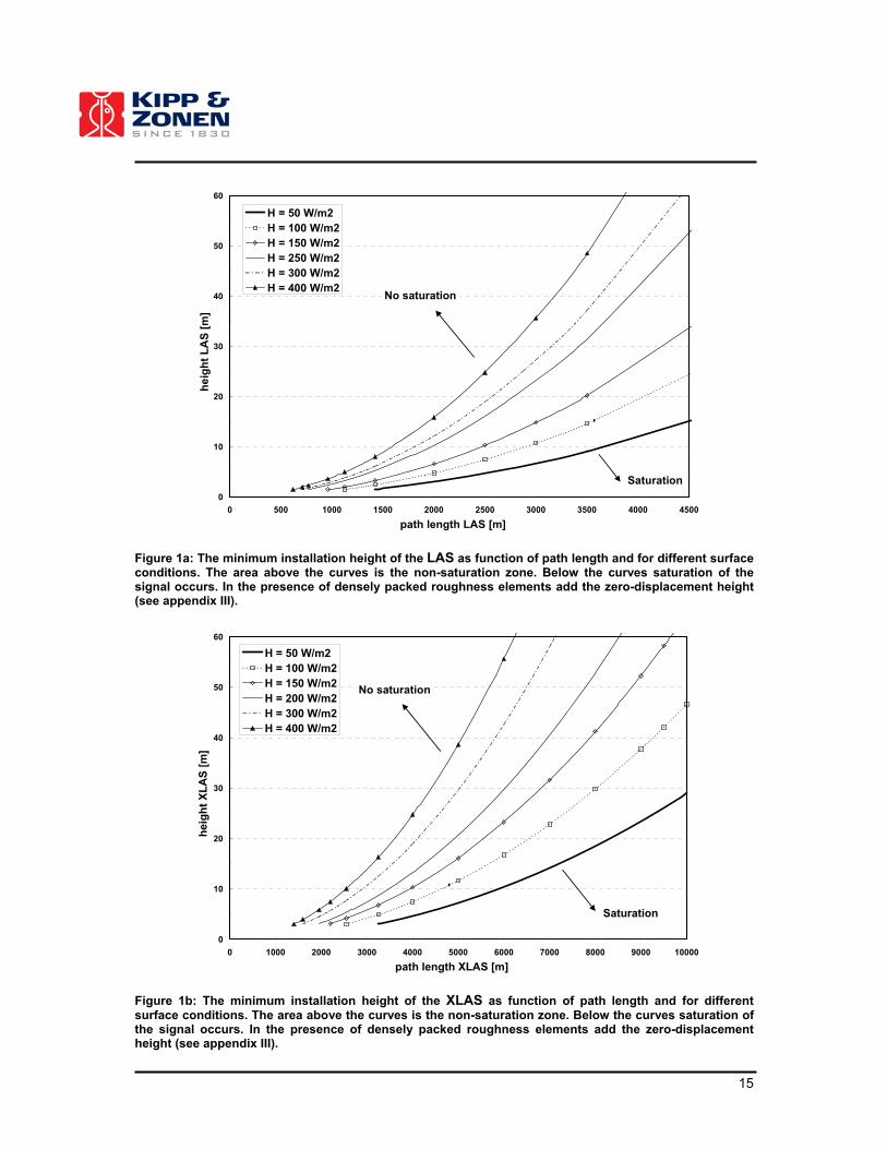
2 values than over wet surfaces where the sensible heat flux is small. In figure 1a,b the minimum height of the LAS and XLAS are given for different surface conditions as a function of the path length. The path length ranges between 250 m and 4.5 km for the LAS and 1 km and 8 km for the XLAS, respectively. The surface conditions range from very dry (H ~ 400 W m-2) to very wet (H ~ 50 W m-2). The area above the curves in the figure is the so-called non-saturation zone. Below the curves saturation will occur. Based on the user’s preferred path length, and the surface conditions of the area of interest, the user must install the LAS and XLAS at a height that lies in the non-saturation zone.
15
0
10
20
30
40
50
60
0 500 1000 1500 2000 2500 3000 3500 4000 4500
path length LAS [m]
heig
ht
LA
S [
m]
H = 50 W/m2
H = 100 W/m2
H = 150 W/m2
H = 250 W/m2
H = 300 W/m2
H = 400 W/m2No saturation
Saturation
Figure 1a: The minimum installation height of the LAS as function of path length and for different surface conditions. The area above the curves is the non-saturation zone. Below the curves saturation of the signal occurs. In the presence of densely packed roughness elements add the zero-displacement height (see appendix III).
0
10
20
30
40
50
60
0 1000 2000 3000 4000 5000 6000 7000 8000 9000 10000
path length XLAS [m]
heig
ht
XL
AS
[m
]
H = 50 W/m2
H = 100 W/m2
H = 150 W/m2
H = 200 W/m2
H = 300 W/m2
H = 400 W/m2
No saturation
Saturation
Figure 1b: The minimum installation height of the XLAS as function of path length and for different surface conditions. The area above the curves is the non-saturation zone. Below the curves saturation of the signal occurs. In the presence of densely packed roughness elements add the zero-displacement height (see appendix III).
16
For example a LAS installed over a relatively wet area (H ~ 100 W m-2) and a path length of 3 km must be installed at a height of 10 - 12 meters or more, according to Figure 1a.
Important: Verify that the LAS and XLAS are operating in the ‘saturation free’ zone.
Important: Determine the effective height of beam of the LAS/XLAS (zLAS) along the path precisely as the sensible heat flux derived from the structure parameter data is very sensitive to the height (see appendix I)! When the area is relatively flat and the beam is parallel to the surface the effective height is easy to determine (ztransmitter = zreceiver = zLAS). For situations that the area is NOT flat or slanted paths it is recommend measuring the height of the beam at several points along the path. By weighing the collected beam heights using the spatial weighting function of the LAS/XLAS (see appendix II) the effective beam height can be derived (see e.g. figure 16). In the presence of densely packed roughness elements (e.g. dense crop or forest) one has to account for the zero-displacement (d) height also (i.e. add d to the minimum height)!
3.3.2 Minimum and maximum height – MOST
In order to derive the surface fluxes of sensible heat from the scintillometer measurements (i.e. Cn
2) we use the so-called Monin-Obukhov Similarity Theory (MOST) (see appendix I). MOST is widely used in the meteorology and is usually applied to the Surface Layer (SL) (and hence is sometimes called Surface Layer Similarity). The SL is roughly the lowest 10% of the Planetary Boundary Layer (PBL). The PBL is directly influenced by the earth’s surface and its depth varies between roughly 100 m to 2 km. In general the PBL increases during the day, when the earth’s surface is heated by the sun, and decreases again during the night. In the SL the variation of fluxes (such as the sensible heat flux H and latent heat flux LvE) is negligible with respect to the magnitude of their value at the surface. Therefore, fluxes measured at a certain elevation in the SL can be considered as being representative for the exchange processes occurring between the earth surface and the atmosphere. The SL can be divided again into the Roughness Sublayer (RS) influenced by the structure of the roughness elements (e.g. plants, trees, buildings etc) and the Constant Flux Layer where fluxes are assumed to be horizontally and vertically constant (due to turbulent mixing). This means that measurement techniques that apply MOST for estimating surface fluxes can be applied only in the Constant Flux Layer. Therefore the LAS/XLAS have to be installed at a height such that it is located above the Roughness Sublayer and is measuring within the Constant Flux Layer. The depth of the SL roughly varies between 20 m to 100 m. The upper level strongly depends on the diurnal cycle of surface heating and cooling (and by the presence of clouds). Like the PBL, the SL increases during the day, as the surface is heated by the sun and is maximum at sun set (~100 m), before is decreases again due to cooling of the surface at night (~20 m). The height of the Roughness Sublayer (and thus lower level of the Constant Flux Layer) depends strongly on the size, form and distribution of the roughness elements. Usually, over tall vegetation, the height of the Roughness Sublayer is taken to be equal to three times the obstacle height (or roughness elements h (see also appendix III)). In case the estimated height of the Roughness Sublayer is smaller than the minimum height of the LAS/XLAS in table 3, take as minimum height the values shown in table 3!
Important: Verify that the LAS and XLAS are measuring in the Constant Flux Layer.
.
17
3.4 THE MOUNTING SUPPORT
The LAS and XLAS can only function properly when the transmitter and receiver unit are precisely optically aligned. By mounting the scintillometer on a stable support, signal loss and regular re-alignment procedures will be avoided. In addition vibrations in the mounting structure must be prevented, which can lead to overestimated Cn
2 values. Important: Always place the LAS/XLAS units on a STABLE (vibration free) construction.
3.5 MOUNTING THE LAS AND XLAS
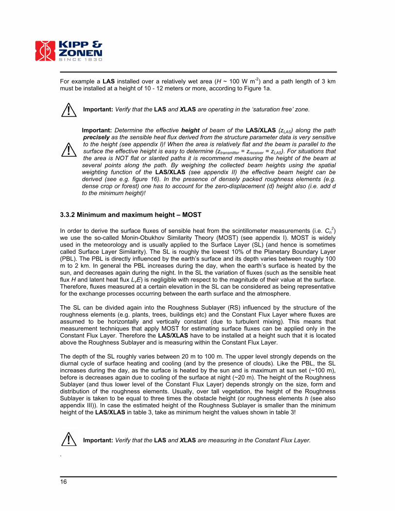
The pan and tilt adjusters of the LAS/XLAS transmitter and receiver are supplied with a bottom flange, which provides simple mounting on the optional tripods (G-3M) using the M16 bolts and washers supplied. The bottom flange can also be fixed to the optional Kipp & Zonen tripod floor stands or to customer-supplied supports using 4� M10 bolts, nuts and washers (not supplied) for each of the transmitter and receiver.
Figure 2: Example of LAS mounted on the optional tripod floor stand.
3.6 ELECTRICAL CONNECTION
3.6.1 Amphenol socket
The LAS/XLAS transmitter and receiver are each provided with a 5 m cable with 10 wires and a shield. At one end of each cable is a 10-way circular Amphenol plug is fitted. These plugs mate with the 10-way circular Amphenol sockets at the receiver and transmitter. The LAS/XLAS can be connected to a computer or data logger. An analogue DC voltage input module with A to D (12 to 16 Bit) converter must be available.
Important: Always measure log Cn2 (UCN2) together with the demodulated signal (UDEMOD).
Although the demodulated carrier signal is not used in the calculations it is an important parameter for monitoring the quality of the Cn
2 measurements.
18
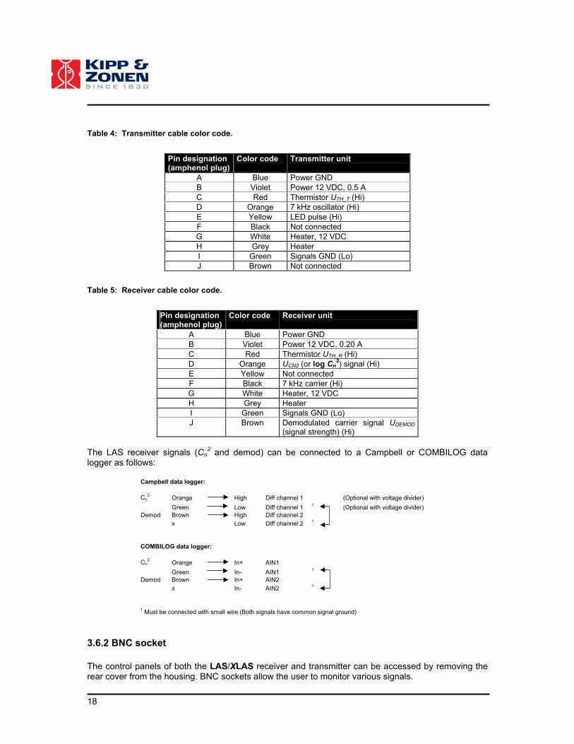
Table 4: Transmitter cable color code.
Pin designation (amphenol plug)
Color code Transmitter unit
A Blue Power GND B Violet Power 12 VDC, 0.5 A C Red Thermistor UTH_T (Hi) D Orange 7 kHz oscillator (Hi) E Yellow LED pulse (Hi) F Black Not connected G White Heater, 12 VDC H Grey Heater I Green Signals GND (Lo) J Brown Not connected
Table 5: Receiver cable color code.
Pin designation (amphenol plug)
Color code Receiver unit
A Blue Power GND B Violet Power 12 VDC, 0.20 A C Red Thermistor UTH_R (Hi) D Orange UCN2 (or log Cn
2) signal (Hi) E Yellow Not connected F Black 7 kHz carrier (Hi) G White Heater, 12 VDC H Grey Heater I Green Signals GND (Lo) J Brown Demodulated carrier signal UDEMOD
(signal strength) (Hi)
The LAS receiver signals (Cn
2 and demod) can be connected to a Campbell or COMBILOG data logger as follows:
Campbell data logger:
Cn2
Orange High Diff channel 1 (Optional with voltage divider)
Green Low Diff channel 1 1 (Optional with voltage divider)Demod Brown High Diff channel 2
x Low Diff channel 2 1
COMBILOG data logger:
Cn2
Orange In+ AIN1
Green In- AIN1 1
Demod Brown In+ AIN2
x In- AIN2 1
1 Must be connected with small wire (Both signals have common signal ground)
3.6.2 BNC socket
The control panels of both the LAS/XLAS receiver and transmitter can be accessed by removing the rear cover from the housing. BNC sockets allow the user to monitor various signals.
19
The BNC socket labeled LED pulse on the control panel of the LAS transmitter can be connected to an oscilloscope to monitor the magnitude of the 7 kHz carrier. This gives an indication of the transmitted waveform and the current being pulsed through the LED emitter. The pulse waveform is square-shaped and is scaled as 1 V equivalent to 1 A. The maximum permissible current is 1 A (when the Current adjust knob is set at maximum), which corresponds to an average current of 0.5 A (duty cycle of 0.5). By connecting an oscilloscope to the BNC socket labeled Carrier on the control panel of the LAS/XLAS receiver the 7 kHz carrier can be monitored, provided that the switch labeled Mode is set at Signal. The waveform should be sinusoidal. If the detector becomes saturated the shape of the wave is clipped and becomes saw-tooth like. When this occurs reduce the LED emitter current. The BNC socket labeled log Cn2 allows the user to monitor UCN2 using a standard DC Voltmeter, provided that the switch labeled Mode is set at Signal. By applying equation 2 the structure parameter of the refractive index of air (Cn
2) can be derived.
3.6.3 Protection circuitry and fuse ratings
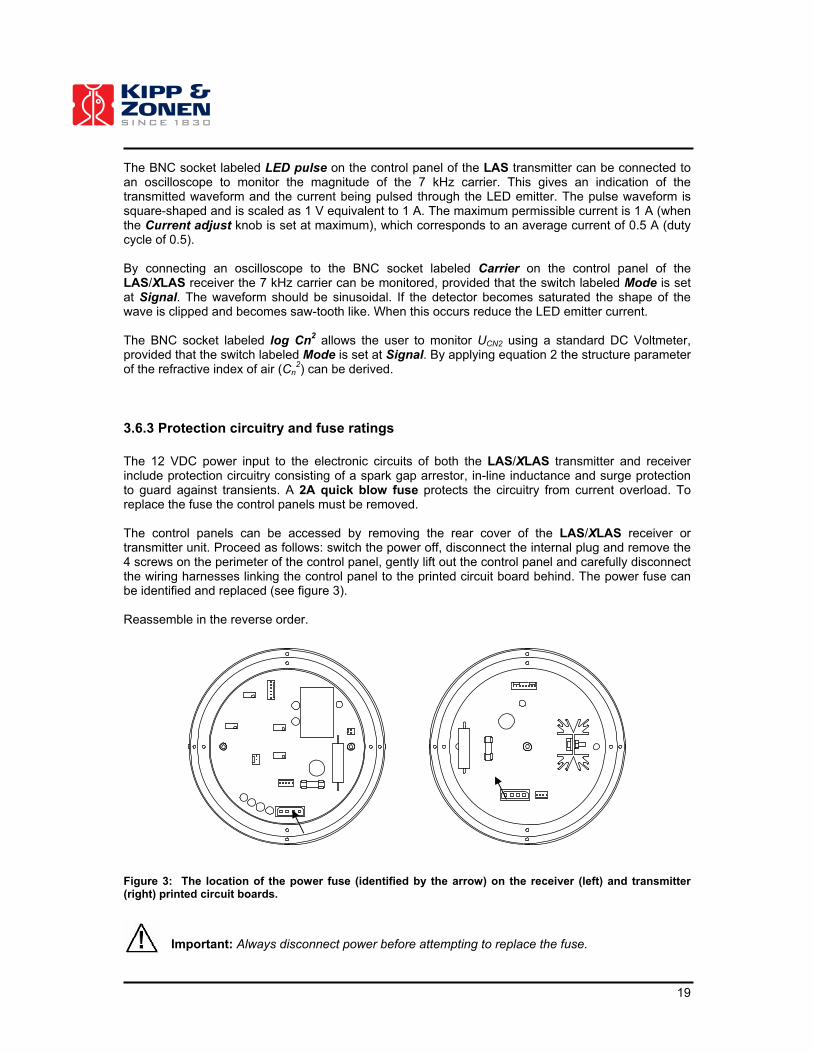
The 12 VDC power input to the electronic circuits of both the LAS/XLAS transmitter and receiver include protection circuitry consisting of a spark gap arrestor, in-line inductance and surge protection to guard against transients. A 2A quick blow fuse protects the circuitry from current overload. To replace the fuse the control panels must be removed. The control panels can be accessed by removing the rear cover of the LAS/XLAS receiver or transmitter unit. Proceed as follows: switch the power off, disconnect the internal plug and remove the 4 screws on the perimeter of the control panel, gently lift out the control panel and carefully disconnect the wiring harnesses linking the control panel to the printed circuit board behind. The power fuse can be identified and replaced (see figure 3). Reassemble in the reverse order.
Figure 3: The location of the power fuse (identified by the arrow) on the receiver (left) and transmitter (right) printed circuit boards.
Important: Always disconnect power before attempting to replace the fuse.

20
3.7 OPTICAL ALIGNMENT
The alignment of the LAS/XLAS at the measurement site is an iterative process for establishing the optimum signal strength for horizontal line-of-sight transmission. The different steps are summarised below. We recommend practice of the alignment procedure at a short range (~ 150 m) first, before proceeding to longer distances. The transmitter and receiver can be rotated around both vertical and horizontal axes. The coarse adjustment of the horizontal alignment (pan) can be done before the bolt(s) that fixes the adjuster bottom flange to the supporting base/structure is (are) completely tightened. Fine pan adjustment can be done with the two horizontal screws with black knobs, which are located just below the case of transmitter or receiver, at the back of the adjuster. For the vertical alignment (tilt), two vertical adjustment bolts are provided, one at the front and one at the rear (see figure 4).
Figure 4: Diagram of pan and tilt adjuster.
Two people should carry out the alignment, one at the receiver and one at the transmitter site. They should be able to communicate either by radio, walkie-talkies or mobile telephones. The transmitter and receiver are mounted at their respective positions. The bolts used to fix the pan and tilt adjusters of the LAS/XLAS to the supporting structures (either a tripod, or something else) are fastened by hand, so that the LAS/XLAS can still be turned around its vertical axis.
1. The telescopes are mounted to the rails on tops of the transmitter and receiver. Note that the telescopes are factory-aligned for each transmitter and receiver and are marked appropriately with either ‘Transmitter’ or ‘Receiver’.
2. The transmitter is adjusted both horizontally (pan) and vertically (tilt) such that the crosshairs of the telescope are centered on the receiver. The same is done for the receiver, relative to the transmitter. Tighten the bolts fixing the pan and tilt adjusters of the LAS/XLAS to the supporting structures (further adjustments can be done with the pan fine adjustment screws).
3. Remove the rear covers of the transmitter and receiver, connect suitable power supplies to both units and switch on. The Power indicator on each control panel should illuminate. Set the switch labeled Mode at the receiver control panel to Signal. At the transmitter side the current is adjusted to a reasonable value with the Current Adjust knob (the dial runs from 0 to 1000). Full scale is approximately 0.5 A (see table 6). For path lengths of about 1 km the current should lie approximately around 0.15 A, whereas for paths of 4.5 km 0.5 A is required. Note that the received signal strength depends on the visibility. If all is well, the analogue meter (Signal Strength) at the control panel of the receiver should give some signal already (to make the meter ten times as sensitive, it can be switched to long range, rather than short range).
Horizontal ‘Pan’ Adjustment (fine)
Vertical ‘Tilt’ Adjustment
21
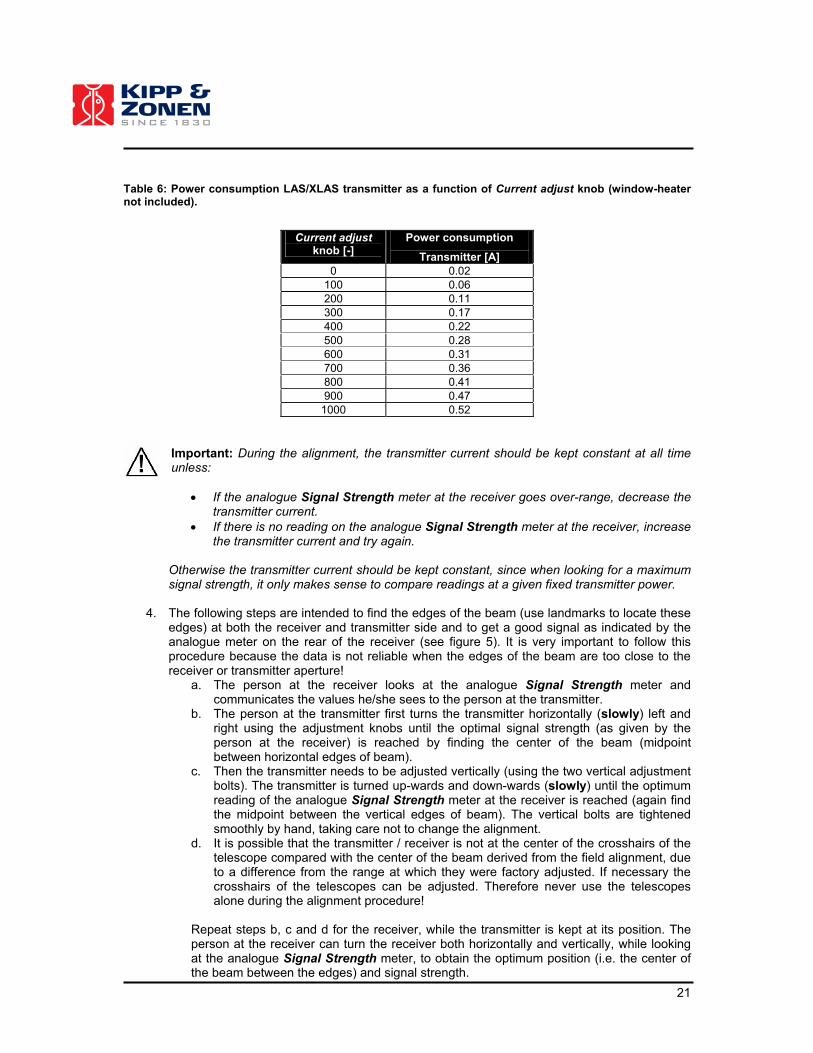
Table 6: Power consumption LAS/XLAS transmitter as a function of Current adjust knob (window-heater not included).
Current adjust
knob [-] Power consumption
Transmitter [A]
0 0.02 100 0.06 200 0.11 300 0.17 400 0.22 500 0.28 600 0.31 700 0.36 800 0.41 900 0.47
1000 0.52
Important: During the alignment, the transmitter current should be kept constant at all time unless:
� If the analogue Signal Strength meter at the receiver goes over-range, decrease the transmitter current.
� If there is no reading on the analogue Signal Strength meter at the receiver, increase the transmitter current and try again.
Otherwise the transmitter current should be kept constant, since when looking for a maximum signal strength, it only makes sense to compare readings at a given fixed transmitter power.
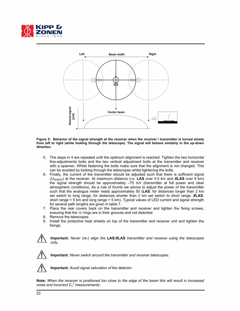
4. The following steps are intended to find the edges of the beam (use landmarks to locate these
edges) at both the receiver and transmitter side and to get a good signal as indicated by the analogue meter on the rear of the receiver (see figure 5). It is very important to follow this procedure because the data is not reliable when the edges of the beam are too close to the receiver or transmitter aperture!
a. The person at the receiver looks at the analogue Signal Strength meter and communicates the values he/she sees to the person at the transmitter.
b. The person at the transmitter first turns the transmitter horizontally (slowly) left and right using the adjustment knobs until the optimal signal strength (as given by the person at the receiver) is reached by finding the center of the beam (midpoint between horizontal edges of beam).
c. Then the transmitter needs to be adjusted vertically (using the two vertical adjustment bolts). The transmitter is turned up-wards and down-wards (slowly) until the optimum reading of the analogue Signal Strength meter at the receiver is reached (again find the midpoint between the vertical edges of beam). The vertical bolts are tightened smoothly by hand, taking care not to change the alignment.
d. It is possible that the transmitter / receiver is not at the center of the crosshairs of the telescope compared with the center of the beam derived from the field alignment, due to a difference from the range at which they were factory adjusted. If necessary the crosshairs of the telescopes can be adjusted. Therefore never use the telescopes alone during the alignment procedure!
Repeat steps b, c and d for the receiver, while the transmitter is kept at its position. The person at the receiver can turn the receiver both horizontally and vertically, while looking at the analogue Signal Strength meter, to obtain the optimum position (i.e. the center of the beam between the edges) and signal strength.
22
Beam width
Center beam
Dem
od
sig
nal
[
mV
]
Signal strength
0
Left Right
Figure 5: Behavior of the signal strength at the receiver when the receiver / transmitter is turned slowly from left to right (while looking through the telescope). The signal will behave similarly in the up-down direction.
5. The steps in 4 are repeated until the optimum alignment is reached. Tighten the two horizontal
fine-adjustments bolts and the two vertical adjustment bolts at the transmitter and receiver with a spanner. Whilst fastening the bolts make sure that the alignment is not changed. This can be avoided by looking through the telescopes whilst tightening the bolts.
6. Finally, the current of the transmitter should be adjusted such that there is sufficient signal (UDEMOD) at the receiver. At maximum distance (i.e. LAS over 4.5 km and XLAS over 8 km) the signal strength should be approximately –75 mV (transmitter at full power and clear atmospheric conditions). As a rule of thumb we advice to adjust the power of the transmitter such that the analogue meter reads approximately 50 (LAS: for distances longer than 2 km set switch to long range, for distances shorter than 2 km set switch to short range; XLAS: short range < 5 km and long range > 5 km). Typical values of LED current and signal strength for several path lengths are given in table 7.
7. Place the rear covers back on the transmitter and receiver and tighten the fixing screws, ensuring that the ‘o’-rings are in their grooves and not distorted.
8. Remove the telescopes. 9. Install the protective heat shields on top of the transmitter and receiver unit and tighten the
fixings.
Important: Never (re-) align the LAS/XLAS transmitter and receiver using the telescopes only.
Important: Never switch around the transmitter and receiver telescopes. Important: Avoid signal saturation of the detector.
Note: When the receiver is positioned too close to the edge of the beam this will result in increased noise and incorrect Cn
2 measurements.

23
Table 7: Typical values for LED current and signal strength as function of the path length (for clear atmospheric conditions!).
Path length
[m] Current adjust
knob [-] UDEMOD [mV]
An. – meter (short range)
An. – meter (long range)
LAS 250 < 10 > -600 80 � LAS 1000 200 -450 60 � LAS 4500 1000 -80 � 30
XLAS 8000 1000 -80 � 30
Table 8: Relation between the signal strength (UDEMOD) and reading of the analogue Signal Strength meter
for different signal strengths (Rdetector = 8M2 �; Rmeter1 = 560 �; Rmeter2 = 5k6 �; no optical filter).
An. – meter
(short range) An. – meter (long range)
UDEMOD [DC-mV]
UCARRIER [AC-mV]
0 < 2 -8 0 10 30 -80 50 20 60 -160 90 30 90 -240 130 40 � -300 175
50 � -375 215
60 � -445 250
70 � -520 290
80 � -600 335
90 � -680 375
100 � -770 415
24
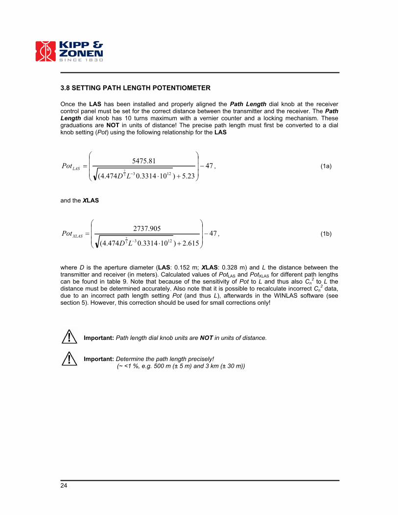
3.8 SETTING PATH LENGTH POTENTIOMETER
Once the LAS has been installed and properly aligned the Path Length dial knob at the receiver control panel must be set for the correct distance between the transmitter and the receiver. The Path Length dial knob has 10 turns maximum with a vernier counter and a locking mechanism. These graduations are NOT in units of distance! The precise path length must first be converted to a dial knob setting (Pot) using the following relationship for the LAS
47
23.5)103314.0474.4(
81.5475
1233
7
����
�
�
���
�
�
���
�LDPotLAS , (1a)
and the XLAS
47
615.2)103314.0474.4(
905.2737
1233
7
����
�
�
���
�
�
���
�LDPotXLAS , (1b)
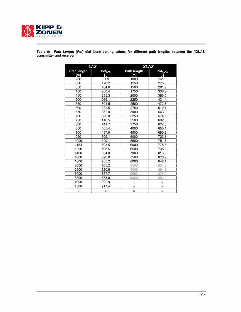
where D is the aperture diameter (LAS: 0.152 m; XLAS: 0.328 m) and L the distance between the transmitter and receiver (in meters). Calculated values of PotLAS and PotXLAS for different path lengths can be found in table 9. Note that because of the sensitivity of Pot to L and thus also Cn
2 to L the distance must be determined accurately. Also note that it is possible to recalculate incorrect Cn
2 data, due to an incorrect path length setting Pot (and thus L), afterwards in the WINLAS software (see section 5). However, this correction should be used for small corrections only!
Important: Path length dial knob units are NOT in units of distance. Important: Determine the path length precisely! (~ <1 %, e.g. 500 m (± 5 m) and 3 km (± 30 m))
25
Table 9: Path Length (Pot) dial knob setting values for different path lengths between the (X)LAS transmitter and receiver.
LAS XLAS Path length
[m] PotLAS
[-] Path length
[m] PotXLAS
[-]
250 91.9 1000 161.9 300 128.2 1250 223.5 350 164.6 1500 281.9 400 200.4 1750 336.2 450 235.3 2000 386.0 500 269.1 2250 431.4 550 301.5 2500 472.7 600 332.5 2750 510.1 650 362.0 3000 543.9 700 390.0 3250 574.5 750 416.5 3500 602.3 800 441.7 3750 627.5 850 465.4 4000 650.4 900 487.9 4500 690.2 950 509.1 5000 723.6
1000 529.1 5500 751.7 1184 593.5 6000 775.5 1200 598.5 6500 796.0 1400 654.0 7000 813.6 1600 698.8 7500 828.9 1800 735.2 8000 842.4 2000 765.2 8500 854.2 2500 820.6 9000 864.6 3000 857.7 9500 873.9 3500 883.8 10000 882.2 4000 902.9 � � 4500 917.4 � �
� � � �

26

27
4. OPERATION After completing the installation the LAS/XLAS (alignment, path length) will be ready for operation. The Cn
2 values can simply be computed from the output signal (UCN2) using the following equation
� �122 210�� CNU
nC . (2)
Cn
2 = structure parameter of the refractive index of air [m-2/3] UCN2 = log Cn2 signal [V]
For example if UCN2 = - 4.0 V, then Cn
2 = 1·10-16 m-2/3. Because of the non-linearity between Cn
2 and the output signal of the LAS/XLAS (UCN2), an interval-averaged UCN2 (e.g. 10 minutes) will not yield the true interval-averaged Cn
2. Therefore we recommend one of the following two options:
1. Measure besides the interval averages of UCN2, the variance of UCN2 (2
2CNU� ) and apply the
following equation for deriving the correct interval-averaged Cn2
� �2
22 15.1122 10 CNUCNUnC
����� . (3)
Cn
2 = structure parameter of the refractive index of air [m-2/3] UCN2 = log Cn2 signal [V]
2
2CNU� = variance of UCN2 [V2]
2. Calculate Cn2 immediately after each measurement cycle (e.g. 1 Hz) and derive the interval-
averaged Cn2 (e.g. 10 minute averages) from the instantaneous Cn
2 values. Because Cn2
values are too small to store in most conventional data acquisition systems (~ 1·10-16) multiply the Cn
2 values by 1·1015 (PULAS). Whether this option can be applied depends on the capability of the data acquisition systems to perform immediate calculations with the measured data. Afterwards the true Cn
2 values can be derived from PUCN2 as follows
15
2
2 10��� CNn PUC . (4)
In appendix IV and V examples are shown for Campbell Scientific (Model CR10X) and Theodor Friedrichs & Co data loggers (COMBILOG 1020).

28
29
5. WINLAS SOFTWARE The following sections provide information about the LAS/XLAS software: WINLAS. WINLAS allows the LAS/XLAS user to derive the surface fluxes of sensible heat from collected LAS data and additional meteorological data, namely air temperature (T), air pressure (P), wind speed (u) and Bowen ratio (�) data. WINLAS calculates the fluxes according to the theory given in appendix I.
5.1 SYSTEM REQUIREMENTS
The minimum computer hardware requirements for WINLAS is a 100 MHz Pentium computer running Windows 95/98/NT/2000/XP/ME, 16 MB of Ram, 10 MB of free hard-disk space (excluding LAS data) and a mouse.
5.2 INSTALLATION
The WINLAS software consists of four files, namely an executable (WINLAS.exe), an initialization file (WINLAS.ini), a help file (WINLAS.chm) and a data-example file (EXAMPLE.txt), which are supplied on a CD. Once the files are copied to a (sub) directory on the PC, WINLAS can be started by double clicking on WINLAS.exe.
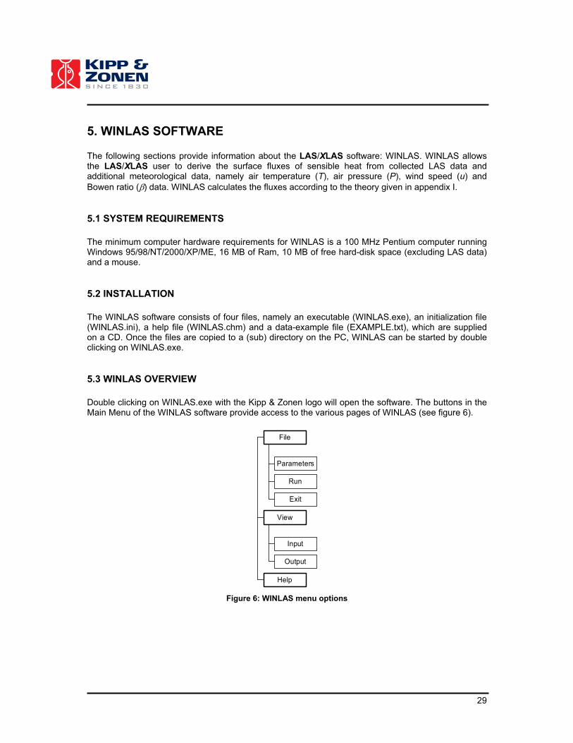
5.3 WINLAS OVERVIEW
Double clicking on WINLAS.exe with the Kipp & Zonen logo will open the software. The buttons in the Main Menu of the WINLAS software provide access to the various pages of WINLAS (see figure 6).
Parameters
Run
Exit
File
Input
Output
View
Help
Figure 6: WINLAS menu options
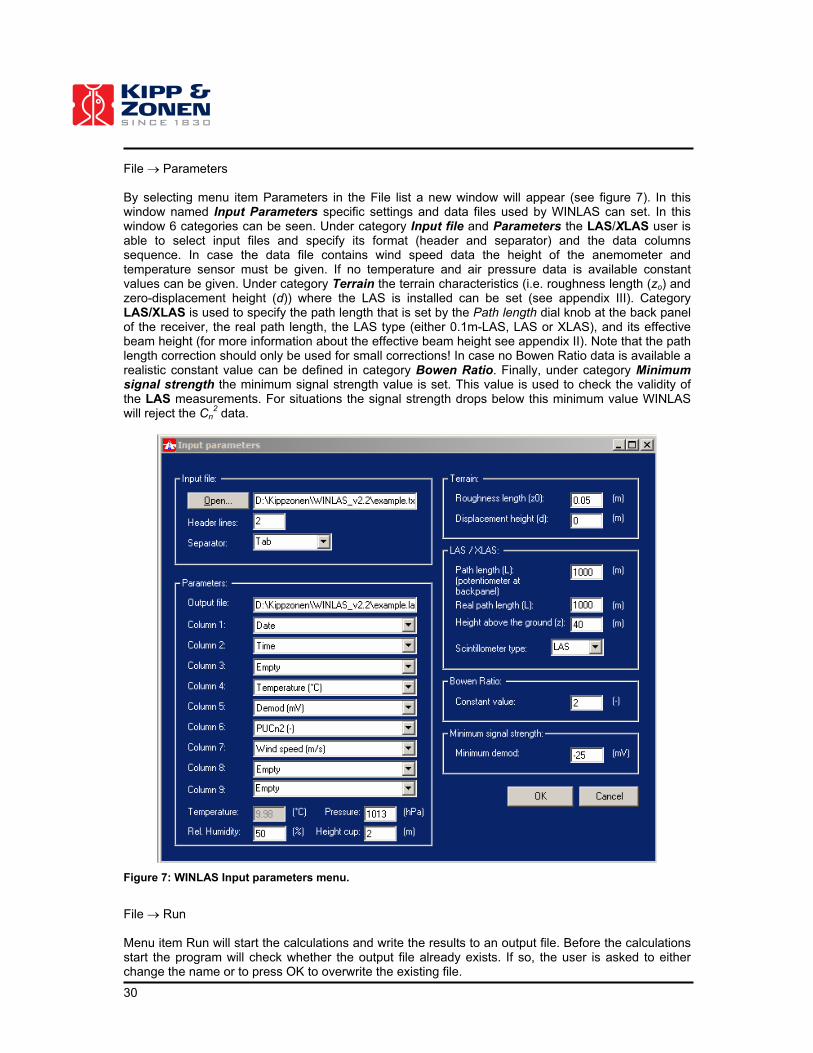
30
File � Parameters By selecting menu item Parameters in the File list a new window will appear (see figure 7). In this window named Input Parameters specific settings and data files used by WINLAS can set. In this window 6 categories can be seen. Under category Input file and Parameters the LAS/XLAS user is able to select input files and specify its format (header and separator) and the data columns sequence. In case the data file contains wind speed data the height of the anemometer and temperature sensor must be given. If no temperature and air pressure data is available constant values can be given. Under category Terrain the terrain characteristics (i.e. roughness length (zo) and zero-displacement height (d)) where the LAS is installed can be set (see appendix III). Category LAS/XLAS is used to specify the path length that is set by the Path length dial knob at the back panel of the receiver, the real path length, the LAS type (either 0.1m-LAS, LAS or XLAS), and its effective beam height (for more information about the effective beam height see appendix II). Note that the path length correction should only be used for small corrections! In case no Bowen Ratio data is available a realistic constant value can be defined in category Bowen Ratio. Finally, under category Minimum signal strength the minimum signal strength value is set. This value is used to check the validity of the LAS measurements. For situations the signal strength drops below this minimum value WINLAS will reject the Cn
2 data.
Figure 7: WINLAS Input parameters menu.
File � Run Menu item Run will start the calculations and write the results to an output file. Before the calculations start the program will check whether the output file already exists. If so, the user is asked to either change the name or to press OK to overwrite the existing file.

31
File � Exit The program WINLAS will be closed and its settings will be saved automatically in WINLAS.ini. View � Input Once an input file is selected in the Parameter menu, the menu item Input under View is enabled. Clicking this menu item will open the input file for viewing and editing. View � Output Once WINLAS has derived the fluxes from an input file the menu item Output is enabled. Clicking this menu item will open the output file for viewing and editing.
5.4 THE INPUT FILE
The data input file should be an ASCII file consisting of columns (with or without a header), which are separated by a comma, semicolon, a space or a tab. The first two data columns should always be a date stamp (or day number, DOY) and a time stamp, followed by LAS/XLAS data (Cn
2 and signal strength) and additional meteorological data (namely T, u, P and �). Header lines are the number of lines that will be skipped by the program before reading the actual data columns. If there is no header this value should be 0.
Important: The maximum allowed number of data columns in the input file is 8, including the Date/DOY and Time columns!
The following LAS and additional meteorological data can be read by WINLAS:
� * Cn2 [m-2/3]
� * UCn2 [V] (i.e. UCN2 of the LAS/XLAS) preferably in combination with VarUCn2 [V2] (i.e. the
variance of UCN2, namely 2
2CNU� ) selected in the following data column. Cn2 is calculated
according to equation 3. � * PUCn2 [-] (i.e. scaled Cn
2, which is stored by the CR10X Campbell program example shown in appendix IV). Cn
2 is calculated according to equation 4. � Signal strength [mV] (i.e. UDEMOD of the LAS/XLAS) � Air temperature (T) [oC] (between -30 and +50 oC) � Air pressure (P) [hPa] (between 950 and 1080 hPa) � Wind speed (u) [m s-1] (between 0 and 100 m s-1) � Bowen ratio (�) [-] (between -10 and +10) � Empty
* CHOOSE ONLY ONE OF THESE THREE OPTIONS!
Important: In case of missing or invalid data the following Dummy value should be used in the input file: -9999. Other dummy values are not accepted by WINLAS.

32
Doy Time UCN2 Demod Var_UCN2 PUCN2 u T[-] [UTC] [V] [mV] [V
2] [-] [m/s] [
oC]
11 600 -3.003 -102.4 0.009 1.0178 2.341 14.9611 610 -3.144 -85 0.014 0.74559 1.869 15.0911 620 -2.774 -46.46 0.038 1.8633 2.353 15.5511 630 -1.612 -11.13 1.55 446.41 3.97 15.9111 640 -2.45 -15.21 0.299 15.556 4.136 16.0711 650 0.179 -1.806 0.028 1590.7 4.102 15.8511 700 0.193 -1.823 0.001 1563.8 3.055 15.9711 710 -0.095 -2.028 0.038 877.43 3.527 16.1611 720 -0.997 -3.004 0.102 130.33 2.815 16.4811 730 -2.362 -25.71 0.254 8.9348 3.117 16.5411 740 -1.861 -6.99 0.001 13.809 2.674 16.7211 750 -1.827 -6.582 0.002 14.989 2.553 17.1811 800 -1.668 -5.105 0.001 21.535 3.214 17.2311 810 -1.837 -7.09 0.061 16.85 2.939 17.6111 820 -2.53 -27.05 0.05 3.409 2.407 17.4711 830 -2.522 -66.5 0.045 3.4621 2.219 17.7211 840 -2.895 -115.4 0.038 1.4077 2.764 18.111 850 -3.116 -159.3 0.01 0.78745 3.681 17.8111 900 -3.224 -200.2 0.024 0.63656 2.513 16.7811 910 -3.185 -220.2 0.019 0.68623 4.335 18.1711 920 -3.265 -227.5 0.016 0.56941 3.687 17.8611 930 -2.875 -229.7 0.037 1.4579 4.88 18.311 940 -2.651 -231.6 0.026 2.3807 4.309 18.1511 950 -2.544 -233.9 0.02 3.0127 4.105 17.6711 1000 -2.639 -232.3 0.009 2.351 3.067 17.5411 1010 -2.504 -238.4 0.024 3.3331 3.882 18.2411 1020 -2.398 -241 0.018 4.1807 4.878 18.2311 1030 -2.438 -236.2 0.013 3.7704 5.279 18.8311 1040 -2.286 -230.5 0.012 5.3446 4.522 18.1411 1050 -2.372 -230.1 0.015 4.4093 4.278 18.911 1100 -2.319 -229.6 0.03 5.1836 4.205 18.4211 1110 -2.367 -229.7 0.019 4.508 4.59 18.9811 1120 -2.281 -229.7 0.016 5.4509 3.323 19.311 1130 -2.327 -227.2 0.013 4.877 3.858 19.1911 1140 -2.323 -226.5 0.014 4.9236 3.239 19.0611 1150 -2.153 -227.4 0.011 7.2483 2.932 18.6111 1200 -2.306 -226.8 0.012 5.1062 3.009 18.4311 1210 -2.285 -226.1 0.03 5.5913 2.958 18.8511 1220 -2.145 -230.5 0.012 7.3962 3.717 18.5311 1230 -2.255 -229.3 0.028 5.9785 4.161 18.93
Figure 8: example of an input file (contains 10-minute averages of LAS and additional data).
Note that the data file in figure 8 contains two columns with Cn
2 information, option1: column 3 combined with column 5 and option 2: column 6. In this case only one of these two options must selected in WINLAS and NOT both. If temperature, air pressure and Bowen ratio data are selected in columns 3 to 8, the input boxes for constant values for temperature, air pressure and Bowen ratio will be disabled. In case no wind speed data is available WINLAS calculates the sensible heat flux using the free convection approach only.

33
5.5 THE OUTPUT FILE
Once an input file is selected, the output file is given the same name with extension .las. The output file is an ASCII file and contains the following data columns:
� Date or Day number (=DOY) � Time � Cn
2 [m-2/3] � Demod [mV] � Hunstable [W m-2] (sensible heat flux, unstable (or day-time) solution) � Hstable [W m-2] (sensible heat flux, stable (or night-time) solution) � Hfree convection [W m-2] (sensible heat flux, free convection solution) � Wind speed [m s-1] � u*unstable [m s-1] (friction velocity, unstable solution) � u*stable [m s-1] (friction velocity, stable solution) � LMO_unstable [m] (Obukhov length, unstable solution) � LMO_stable [m] (Obukhov length, stable solution) � Bowen ratio [-] � Air temperature [oC] � Relative humidity [%] � Air pressure [hPa] � Air density [kg m-3] � Comment saturation (“no saturation”, “-“ or “possible saturation”)

34
35
6. MAINTENANCE To be certain that the quality of the data is of high standard, care must be taken with the maintenance of the LAS/XLAS. Regular cleaning of the windows and checking the alignment (using telescopes) will prevent unnecessary signal attenuation and data loss. Also periodically check the condition of all cables and connectors.
Important: Always keep power connected and switched on to the LAS/XLAS transmitter and receiver when they are placed outside to prevent condensation.
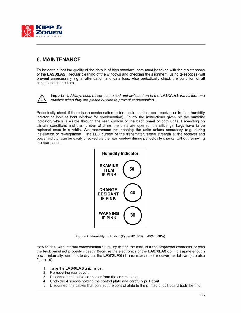
Periodically check if there is no condensation inside the transmitter and receiver units (see humidity indictor or look at front window for condensation). Follow the instructions given by the humidity indicator, which is visible through the rear window of the back panel of both units. Depending on climate conditions and the number of times the units are opened, the silica gel bags have to be replaced once in a while. We recommend not opening the units unless necessary (e.g. during installation or re-alignment). The LED current of the transmitter, signal strength at the receiver and power indictor can be easily checked via the rear window during periodically checks, without removing the rear panel.
Humidity Indicator
50
CHANGEDESICANT
IF PINK
WARNINGIF PINK
EXAMINEITEM
IF PINK
40
30
Figure 9: Humidity indicator (Type B2, 30% .. 40% .. 50%).
How to deal with internal condensation? First try to find the leak. Is it the amphenol connector or was the back panel not properly closed? Because the electronics of the LAS/XLAS don’t dissipate enough power internally, one has to dry out the LAS/XLAS (Transmitter and/or receiver) as follows (see also figure 10):
1. Take the LAS/XLAS unit inside. 2. Remove the rear cover. 3. Disconnect the cable connector from the control plate. 4. Undo the 4 screws holding the control plate and carefully pull it out 5. Disconnect the cables that connect the control plate to the printed circuit board (pcb) behind

36
6. Remove the six screws at the front holding the window assembly to the housing. Be careful not to loose the screws and the rubber O-rings (6 small and 1 large). For details see figure 10.
7. Gently lift out the lens/heater ring assembly and disconnect the power cable from the heater to the bullet. Do NOT disassemble the housing any further because this might affect the optical alignment of the transmitting LED and/or receiving photo-diode!
Dry the inside of the housing as much as possible and clean off any surface corrosion. Clean the window and Fresnel lens using a dry tissue (and/or dust free blower). If the lens is still dirty then a mild soap solution can be used. The Fresnel lens is a moulded plastic component - do NOT use solvents to clean it! Leave the housing open to dry for a couple of hours/days (depending on room temperature) and reassemble in the reverse order. Note that the Fresnel lens is mounted with the grooved surface facing outwards towards the window. Clean any hard grease off the o-ring seals and apply silicone grease before reassembly (if not available Vaseline will do). The front and rear covers screw down to make metal-to-metal contact with the housing when the o-rings are properly compressed.
Rear cover Window
Window assembly
Screws (6�)
O-rings
Fresnel lens
Lens/heater ring
assembly
Connector
for heater ringControl plate
Cable connector
Figure 10: Window - Fresnel - Heating ring assembly.

37
7. CALIBRATION
7.1 ON-SITE CALIBRATION CHECK
The purpose of the electronics in the LAS/XLAS receiver unit is to provide real-time values for Cn
2 but scaled in voltage units, which can be recorded by data acquisition systems. The electronics perform the following steps: detection with feed-back circuit to remove slow ambient fluctuations; demodulation of the carrier signal; low-pass filtering at 400 Hz to remove high-frequency noise; producing the logarithm of the signal intensity; removing any offsets; path length correction (i.e. adjustment of Gain); filtering the scintillation bandwidth between 0.2 Hz and 400 Hz; calculation of the variance of the conditioned signal. In addition to the analogue pre-processing, calibration circuitry provides the user a quick on-site check of the performance of the real-time Cn
2 calculations. By setting the receiver control panel switch labelled Mode to Calibration a reference signal of a known modulation and carrier frequency is sent through the analogue processing circuitry. This reference signal consists of a 7 kHz (± 0.7 kHz) square-wave carrier modulated by a 10 Hz (± 1 Hz) square-wave with a modulation depth of 50%. This reference signal can be monitored at the BNC socket labelled Carrier with an oscilloscope. Due to additional filters this reference signal is slightly distorted. However, the modulated signal is still recognisable. By adjusting the Path Length dial knob of the LAS to a setting of 593.5 (equal to L = 1184 m) and for the XLAS a setting of 414.1 (equal to L = 2152 m), zero volts should be measured at BNC socket log Cn2. If the signal is not 0 V (� 15 mV) after 1 hour of warm-up time, the receiver electronics need to be recalibrated. In table 10 a range of output values are given for different Path Length dial knob settings when set in Calibration mode.
Important: When performing a calibration check the LAS/XLAS receiver should be connected to a stable power supply and the environmental temperature must be constant at close to room temperature.
Table 10: Output signal UCN2 at BNC socket (of LAS/XLAS) as a function of the Path Length dial knob setting (in Calibration mode) at constant room temperature.
LAS XLAS
PotLAS [-]
UCN2 at BNC [mV]
PotXLAS
[-] UCN2 at BNC
[mV] 200 1415 200 813 300 1004 300 402 400 650 400 48 500 316 414 0.0
594 0.0 500 -286 700 -398 600 -626 800 -859 700 -1000 884 -1415 800 -1462
38
7.2 RECALIBRATION
The electronics of the LAS/XLAS receiver unit can change with time and with temperature. Therefore periodic checking of the electronic (see Section 6.1) is advised. If the signal is not within � 15 mV of the values given in table 10 for different Path Length knob settings (check at least 5 different pot settings) the receiver electronics need to be recalibrated. To return a LAS/XLAS to Kipp & Zonen for recalibration the use of the recalibration form at the end of this manual is strongly recommended.
7.3 CALIBRATION PROCEDURE AT KIPP & ZONEN
7.3.1 Calibration procedure RMS-circuits
The receiver electronics contain two RMS-circuits that operate in logarithmic mode. The purpose of the first RMS-circuit is to obtain the log of the received signal intensity. This circuit is calibrated for an arbitrary zero point (offset) and a fixed gain, using two reference voltages of 1.000 V and 0.100 V. The purpose of the second RMS-circuit is to calculate the RMS of the amplified and filtered log intensity fluctuations (i.e. the conditioned signal). As the first RMS-circuit, the second circuit also requires calibration for offset and gain. Because both RMS-circuits operate in log-mode an extra temperature-dependant resistor is added, which compensates for the temperature dependence of the (dB) output of the RMS IC’s. Therefore the electronics require at least 1-hour warm-up time.
7.3.2 Calibration path length
For the calibration of the Path Length dial knob setting an artificial signal is used with a carrier frequency of ~ 7 kHz, which is amplitude modulated with a block signal with a frequency of ~ 10 Hz and a modulation depth of 50%. This signal is directly fed to the demodulator unit (see also Paragraph 7.1).
39
8. SOLVING PROBLEMS The LAS/XLAS is designed for both long and short periods of operation with little operator maintenance. However, if a problem occurs that cannot be corrected using the standard operating information supplied in the preceding sections of this manual, use the information in this chapter to identify and solve the problem. If the problem cannot be corrected after reviewing the information in the following section, contact Kipp & Zonen. When contacting Kipp & Zonen with technical assistance questions, ensure that you have the following information readily available to aid the technician in solving your problem:
� The model number and serial number of the LAS/XLAS. This information is listed on the identification labels, located on the pan and tilt adjusters of the LAS/XLAS transmitter and receiver.
If you cannot solve the problem by the steps on the following pages, please contact Kipp & Zonen. Kipp & Zonen B.V. P.O. Box 507 2600 AM Delft The Netherlands T: +31 (0)15 275 5210 F: +31 (0)15 262 0351 E: [email protected] Web: www.kippzonen.com
8.1 PROBLEM CHECK-LIST
Check the items in the following list. If these do not help, see the following section on troubleshooting. Check that:
� Power is supplied to both the LAS/XLAS transmitter and receiver unit. � The data cables are correctly connected to the data logger or data acquisition unit.
8.2 TROUBLESHOOTING
Table 11: Troubleshooting.
Problem Corrective action
LED indicator on back panel is off Check the power fuse, see Paragraph 3.6.3 Check wires
The receiver has no signal � Check power to transmitter and receiver units � Check if windows are clean (and lenses) and there is
no internal condensation (see section 6 for instructions)� Check alignment (using telescopes) � Check for obstacles in the path of the beam � Check the performance of the transmitter electronics at
the BNC socket labeled LED pulse � Check the performance of the real-time Cn
2 calculations of the receiver electronics by setting the receiver to Calibration mode

40
41
APPENDIX I – THEORY SCINTILLATION TECHNIQUE When an electro-magnetic (EM) beam of radiation propagates through the atmosphere it is distorted by a number of processes. These processes remove energy from the beam and lead to attenuation of the signal. The most serious mechanism that influences the propagation of EM radiation is small fluctuations in the refractive index of the air (n). These refractive index fluctuations lead to intensity fluctuations, which are known as scintillations. A scintillometer is an instrument that can measure the ‘amount’ of scintillations by emitting a beam of light over a horizontal path. The scintillations ‘seen’ by the instrument can be expressed as the structure parameter of the refractive index of air (Cn
2), which is a representation of the ‘turbulent strength’ of the atmosphere. The turbulent strength describes the ability of the atmosphere to transport scalars, such as heat, humidity and other species (dust particles, atmospheric gases). For a Large Aperture Scintillometer (LAS/XLAS) with equal transmitting and receiving apertures the relationship between the measured variance of the natural logarithm of intensity fluctuations (�lnI
2) and the structure parameter is as follows (Wang et al., 1978)
33/72
ln
2 12.1 �� LDC In � , (5)
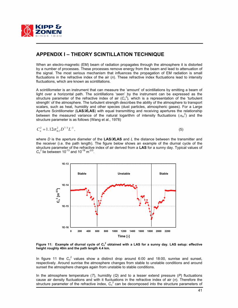
where D is the aperture diameter of the LAS/XLAS and L the distance between the transmitter and the receiver (i.e. the path length). The figure below shows an example of the diurnal cycle of the structure parameter of the refractive index of air derived from a LAS for a sunny day. Typical values of Cn
2 lie between 10-13 and 10-18 m-2/3.
1E-16
1E-15
1E-14
1E-13
0 200 400 600 800 1000 1200 1400 1600 1800 2000 2200
Time [-]
Cn
2 [
m-2
/3]
UnstableStable Stable
Figure 11: Example of diurnal cycle of Cn2 obtained with a LAS for a sunny day. LAS setup: effective
height roughly 40m and the path length 4.4 km.
In figure 11 the Cn
2 values show a distinct drop around 6:00 and 18:00, sunrise and sunset, respectively. Around sunrise the atmosphere changes from stable to unstable conditions and around sunset the atmosphere changes again from unstable to stable conditions. In the atmosphere temperature (T), humidity (Q) and to a lesser extend pressure (P) fluctuations cause air density fluctuations and with it fluctuations in the refractive index of air (n). Therefore the structure parameter of the refractive index, Cn
2 can be decomposed into the structure parameters of
42
temperature CT2, humidity CQ
2 and the covariant term CTQ as follows (neglecting pressure fluctuations) (Hill et al., 1980)
2
2
2
2
2
22
2Q
QTQ
QTT
Tn C
Q
AC
QTAA
CT
AC ��� . (6)
AT and AQ are functions of the wavelength and the mean values of temperature, absolute humidity and atmospheric pressure and thus represent the relative contribution of each term to Cn
2. In the visible and near-infrared wavelength region of the EM spectrum AT and AQ are defined as follows (Andreas, 1988)
QRTPA vT
66 10126.01078.0 �� �����
������ , (7)
QRA vQ610126.0 ���� , (8)
where Rv is the specific gas constant for water vapour (461.5 J K-1 kg-1). Typical values for AT and AQ, for ‘normal atmospheric’ conditions (P = 1�105 Pa, T = 288 K and Q = 0.012 kg m-3), are –0.27�10-3 and –0.70�10-6, respectively. Because AT is much larger than AQ the contribution of humidity related scintillations is much smaller than temperature related scintillations, i.e. the near-infrared LAS/XLAS is primarily sensitive to temperature related scintillations. Therefore a simplified expression can be derived, which makes it possible to derive CT
2 from Cn2 as follows (Wesely, 1976)
2
2
2
22 03.0
1 ���
����
���
�TT
n CTAC or
2
2
2
2
62 03.0
11078.0
���
����
����
�
����
� ���
�
�Tn CT
PC , (9)
where � is the Bowen ratio, which is a correction for term for humidity related scintillations. The Bowen ratio is defined as the ratio between the sensible heat (H) and latent heat flux (LvE), i.e. � = H/LvE. When the surface conditions are dry H is larger than LvE, resulting in high � values (> 3). This means that the correction term in the latter equation is small. Over wet surfaces � is small (< 0.5), which means that a significant amount of scintillations are caused by humidity fluctuations, resulting in a large correction. Thus when the surface conditions are very dry, CT
2 is directly proportional to Cn2
2
2
22
TT
n CTAC � or
2
2
2
62 1078.0
Tn CT
PC ���
����
� ���
�
. (10)
Once CT
2 is known, the sensible heat flux (H) can be derived from similarity relationships that have been derived for CT
2 which are based on the Monin-Obukhov Similarity Theory (MOST) (Wyngaard et al., 1971)
� � � �02
*
3/22
����
����
� ��
�MO
MO
LAST
LAST LL
dzfT
dzC, (11)
where d is the zero-displacement height (see appendix III), zLAS the effective height of the scintillometer beam above the surface (Hartogensis et al., 2003), T* is a temperature scale defined as
*
* ucHTp�
�� , (12)

43
and LMO is the Obukhov length
*
2
*
TgkTuLv
MO � , (13)
where � is the density of air (� 1.2 kg m-3), cp the specific heat of air at constant pressure (� 1005 J kg-
1 K-1), kv the von Kármán constant (� 0.40), g the gravitational acceleration (� 9.81 m s-2) and u* the friction velocity. The universal stability function fT is defined as follows for unstable (day-time, LMO < 0)
� �01
3/2
21 ����
����
� �����
�
����
� ��
MOMO
LASTT
MO
LAST L
Ldz
ccL
dzf , (14)
where cT1 = 4.9 and cT2 = 6.1 and for stable (night-time, LMO > 0) conditions as
� �01
3/2
31 ���
�
�
��
�
����
����
� �����
�
����
� �MO
MO
LASTT
MO
LAST L
Ldz
ccL
dzf , (15)
where cT3 = 2.2 (see Andreas, 1988; De Bruin et al., 1993; Wyngaard et al., 1971).
Important: There is no consensus about the stability function for stable (night-time) conditions!
In order to derive H from CT
2, the friction velocity (u*) is required. The friction velocity can be obtained from additional wind speed data (u) and an estimate of the surface roughness (z0) (Panofsky and Dutton, 1984) (see appendix III)
���
����
� ���
�
����
� � ���
�
����
� ��
OMm
OM
um
u
v
Lz
Ldz
zdz
uku0
0
*
ln
, (16)
where zu is the height at which the wind speed is measured and m is the integrated stability function for momentum defined as (for unstable conditions (day-time))
� � � �02
arctan22
1ln
2
1ln2
2
�����
� !
" ����
� !" �
����
����
� MO
MOm LxxxLz #
, (17)
with
4/1
161 ���
����
���
MOLzx , (18)
or (stable conditions (night-time))
44
� �05 ������
����
� MO
MOMOm L
Lz
Lz
. (19)
In summary, Cn
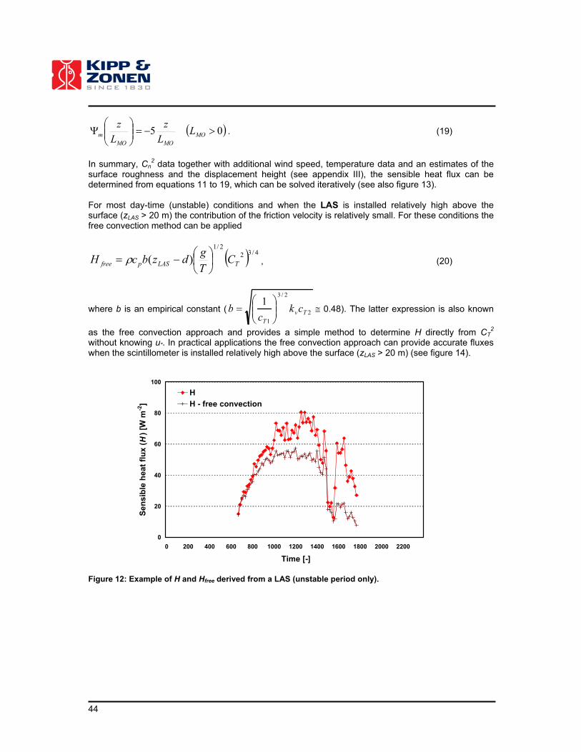
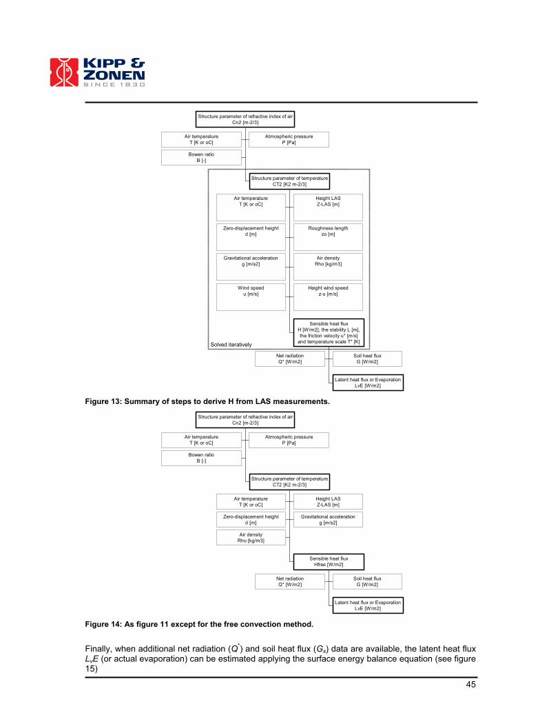
2 data together with additional wind speed, temperature data and an estimates of the surface roughness and the displacement height (see appendix III), the sensible heat flux can be determined from equations 11 to 19, which can be solved iteratively (see also figure 13). For most day-time (unstable) conditions and when the LAS is installed relatively high above the surface (zLAS > 20 m) the contribution of the friction velocity is relatively small. For these conditions the free convection method can be applied
� � 4/32
2/1
)( TLASpfree CTgdzbcH ���
����� � , (20)
where b is an empirical constant ( 2
2/3
1
1Tv
T
ckc
b ���
����
�� $ 0.48). The latter expression is also known
as the free convection approach and provides a simple method to determine H directly from CT2
without knowing u*. In practical applications the free convection approach can provide accurate fluxes when the scintillometer is installed relatively high above the surface (zLAS > 20 m) (see figure 14).
0
20
40
60
80
100
0 200 400 600 800 1000 1200 1400 1600 1800 2000 2200
Time [-]
Se
ns
ible
he
at
flu
x (
H)
[W m
-2]
H
H - free convection
Figure 12: Example of H and Hfree derived from a LAS (unstable period only).
45
Solved iteratively
Air temperatureT [K or oC]
Atmospheric pressureP [Pa]
Bowen ratioB [-]
Air temperatureT [K or oC]
Height LASZ-LAS [m]
Zero-displacement heightd [m]
Roughness lengthzo [m]
Gravitational accelerationg [m/s2]
Air densityRho [kg/m3]
Wind speedu [m/s]
Height wind speedz-u [m/s]
Net radiationQ* [W/m2]
Soil heat fluxG [W/m2]
Latent heat flux or EvaporationLvE [W/m2]
Sensible heat fluxH [W/m2], the stability L [m],the friction velocity u* [m/s]
and temperature scale T* [K]
Structure parameter of temperatureCT2 [K2 m-2/3]
Structure parameter of refractive index of airCn2 [m-2/3]
Figure 13: Summary of steps to derive H from LAS measurements.
Air temperatureT [K or oC]
Atmospheric pressureP [Pa]
Bowen ratioB [-]
Air temperatureT [K or oC]
Height LASZ-LAS [m]
Zero-displacement heightd [m]
Gravitational accelerationg [m/s2]
Air densityRho [kg/m3]
Net radiationQ* [W/m2]
Soil heat fluxG [W/m2]
Latent heat flux or EvaporationLvE [W/m2]
Sensible heat fluxHfree [W/m2]
Structure parameter of temperatureCT2 [K2 m-2/3]
Structure parameter of refractive index of airCn2 [m-2/3]
Figure 14: As figure 11 except for the free convection method.
Finally, when additional net radiation (Q*) and soil heat flux (Gs) data are available, the latent heat flux LvE (or actual evaporation) can be estimated applying the surface energy balance equation (see figure 15)

46
sv GELHQ ���* (21)
-100
0
100
200
300
400
500
600
700
0 200 400 600 800 1000 1200 1400 1600 1800 2000 2200
Time [-]
Flu
x d
en
sit
y [
W m
-2]
Q* Gs H-LAS LvE
Figure 15: Example of time series of net radiation, soil heat flux, sensible heat flux and latent heat flux.
Complete list of required data/information for deriving sensible heat fluxes:
� LAS/XLAS – mean of Cn2 (derived from UCN2)
� LAS/XLAS – mean of signal strength (or Udemod) � LAS/XLAS – variance of signal strength (or Udemod) � LAS/XLAS – path length (L) � LAS/XLAS – average (effective) beam height (zLAS) (see appendix II) � Zero-displacement height (d) (see appendix III) � Air pressure (P) � Air temperature (T) � Wind speed (u) � Bowen ratio (�) � Height(s) of cup anemometer(s) (zu) � Surface roughness (i.e. roughness length) of source area LAS/wind speed measurements (zo)
(see appendix III) Other useful meteorological data:
� Radiation data (Global radiation, net radiation) � Soil heat flux data � Wind direction � Rainfall
47
References Andreas, E.L.: 1988, ‘Estimating Cn
2 over Snow and Sea Ice from Meteorological Data’, J. Opt. Soc. Am. 5, 481-495. Andreas, E.L.: 1990, Selected Papers on Turbulence in a Refractive Medium, SPIE Milestone Series 25, SPIE - The International Society for Optical Engineering, Bellingham, 693 pp. De Bruin, H.A.R., Kohsiek, W. and Van den Hurk, B.J.J.M.: 1993, ‘A Verification of Some Methods to Determine the Fluxes of Momentum, Sensible Heat and Water Vapour using Standard Deviation and Structure Parameter of Scalar Meteorological Quantities’, Boundary-Layer Meteorol. 63, 231-257. Hartogensis, O.K., Watts, C.J., Rodriguez, J-C. and De Bruin, H.A.R.: 2003, ‘Derivation of an Effective Height for Scintillometers: La Poza Experiment in Northwest Mexico’, J. Hydro-Meteorol. 4, 915-928. Hill, R.J., Clifford, S.F. and Lawrence, R.S.: 1980, ‘Refractive Index and Absorption Fluctuations in the Infrared Caused by Temperature, Humidity and Pressure Fluctuations’, J. Opt. Soc. Am. 70, 1192-1205. Panofsky, H.A. and Dutton, J.A.: 1984, Atmospheric Turbulence: Models and Methods for Engineering Applications, J. Wiley, 397 pp. Wang, T.I., Ochs, G.R., and Clifford, S.F.: 1978, ‘A Saturation-Resistant Optical Scintillometer to Measure Cn
2’, J. Opt. Soc. Am. 69, 334-338. Wesely, M.L.: 1976, ‘The Combined Effect of Temperature and Humidity on the Refractive Index’, J. Appl. Meteorol. 15, 43-49. Wyngaard, J.C., Izumi, Y., and Collins Jr., S.A.: 1971, ‘Behaviour of the Refractive Index Structure Parameter Near the Ground’, J. Opt. Soc. Am. 61, 1646-1650.

48

49
APPENDIX II – PATH-WEIGHTING FUNCTION LAS/XLAS The LAS/XLAS provides a measure of the structure parameter of the refractive index of air (Cn
2), weighted over the path length (L). For equal sized transmitter and receiver apertures this path-weighting function is symmetrical bell-shaped having a centre maximum and tapering to zero at the transmitter and receiver end (see figure 16). This means that the LAS/XLAS is most sensitive in the middle of its path. In figure 17 an example is shown how the weighting function has to be used in order to estimate the precise height of the beam of the LAS/XLAS above the surface for non-flat areas. For further details the reader is referred to Hartogensis et al. (2003).
0
0.005
0.01
0.015
0.02
0.025
0 0.2 0.4 0.6 0.8 1
normalised position u [-]
Weig
ht
[%]
Total area = 100%
normalised position weight0 0.000
0.05 0.0020.1 0.0090.15 0.0180.2 0.0310.25 0.0460.3 0.0620.35 0.0790.4 0.0930.45 0.1040.5 0.1080.55 0.1040.6 0.0930.65 0.0790.7 0.0620.75 0.0460.8 0.0310.85 0.0180.9 0.0090.95 0.002
1 0.000
Figure 16: The path-weighting function of the (X)LAS.
0
10
20
30
40
50
60
70
0 0.1 0.2 0.3 0.4 0.5 0.6 0.7 0.8 0.9 1
normalised position [-]
he
igh
t [m
]
0
0.005
0.01
0.015
we
igh
t [%
]
surface
beam - LAS
weighting function - LAS
Transmitter
Receiver
Figure 17: Example of a LAS setup over a non-flat area. Based on the elevation map and the path-weighting function an effective LAS height of 46 m was found.

50

51
APPENDIX III – ROUGHNESS LENGTH & DISPLACEMENT HEIGHT The roughness length (z0) The aerodynamic roughness length or surface roughness (z0) is an expression for the roughness of the earth’s surface. It affects the intensity of mechanical turbulence and the fluxes of sensible heat (H), latent heat (LvE) and momentum above the surface. The roughness length depends on the surface (or terrain) characteristics. For example a grassy plain has a smaller roughness length than an area with many trees and buildings. The surface roughness is loosely related to the typical height (h) of closely spaced surface obstacles, often called roughness elements (e.g. water waves, trees, buildings, blades of grass). It depends on the distribution as well as the height of roughness elements (h).
DENSE:
- low roughness length (z0)- high zero-displacement height (d)
dh
SPARSE:
- high roughness length (z0)- low zero-displacement height (d)
d
h
Figure 18: Dependence of the roughness length and zero-displacement height on height and density of roughness elements (e.g. trees).
In table 12 eight different terrain classifications are given plus their typical roughness length.
Table 12: Terrain classifications.
Classification
No. Name Roughness length [m]
Landscape features
1 Sea 0.0002 Open water, tidal flat, snow with fetch above 3 km 2 Smooth 0.005 Featureless land, ice 3 Open 0.03 Flat terrain with grass or very low vegetation, airport runway 4 Roughly open 0.1 Cultivated area, low crops, obstacles of height h separated
by at least 20h 5 Rough 0.25 Open landscape, scattered shelter belts, obstacles
separated by 15h or so 6 Very rough 0.5 Landscape with bushes, young dense forest etc separated
by 10h or so 7 Closed 1.0 Open spaces comparable with h, e.g. mature forest, low-
rise built-up area 8 Chaotic � 2.0 Irregular distribution of large elements, e.g. city center, large
forest with clearings
52
When the LAS/XLAS are installed over natural landscapes, which are mostly heterogeneous (and a path length of several kilometers) we recommend using table 12 for determining a representative roughness length, if necessary focus on the area in the middle of the path of the LAS/XLAS (most important area, see appendix II). In case the LAS/XLAS are installed over a relative homogeneous area (e.g. a (dense) agricultural field or (dense) forest) it is best to apply a simple rule of thumb:
hz 1.00 � (22)
The zero-displacement height (d) If the area surrounding the LAS/XLAS site consists of roughness elements that are packed very closely together like a dense forest or a dense crop, the top of those elements begin to act like a displaced surface, which is known as the zero-displacement height (d). It is difficult to determine the zero-displacement height. The only proper way to derive the zero-displacement height is from wind profile data. There is simple rule of thumb to derive the displacement height from the crop height:
hd 7.0� (23) However, note that this rule of thumb is not accurate, especially when the crop/forest is not densely packed! In case the roughness elements are not closely packed (see figure 18 (left)) we recommend not using a zero-displacement height (i.e. d = 0). Additional comments/suggestions During daytime conditions with high solar insolation and when the LAS/XLAS are installed relatively high above the surface (> 20 m) the free convection method can be applied (see appendix I). Under those conditions the importance of the roughness length is small, meaning that the sensible heat flux (H) is not very sensitive to changes in z0. However, during nighttime periods the roughness length becomes very important and can have large effects on the sensible heat flux (and also LvE). In case one has to apply a zero-displacement height it might be necessary to spatially weight d also using the weighting function of the LAS/XLAS (see appendix II). In case the zero-displacement is difficult to determine (as roughness elements are not densely packed), one can minimize the (relative) effect of d on the sensible heat flux by installing the LAS/XLAS higher above the surface.

53
APPENDIX IV – HEATER AND THERMISTOR Both the LAS/XLAS transmitter and the receiver units have an integral heater ring for keeping the Fresnel lens and window clear of dew/condensation/snow. The heater of the LAS is self-regulating working to maintain a constant 55 °C temperature the ring will initially draw more than 1A current when first switched on. At around 22 °C room temperature the heater resistance is 17 ohms. Power to the ring is independent of the other electronics and the user can decide whether this higher power demand mode is necessary, particularly if remote site operation is to be considered. The heater of the XLAS is not self-regulating. Instead it constantly draws 1.2A current. The heater ring is in thermal contact with the Fresnel lens and the front window but electrically insulated from the body of the LAS/XLAS. This assembly connects to the printed circuit boards mounted on the transmitter and receiver bullets. These connectors are 4-way providing an option for signal sensing a thermistor mounted on the heater ring assembly. Ambient temperature inside the LAS/XLAS receiver and transmitter units are monitored by NTC thermistors connected to the printed circuit boards and in thermal contact with the bullet. This thermistor forms half of a voltage divider and a scaled voltage output is available at the internal and external bulkhead sockets. The calibration formulae for the transmitter and receiver units are as follows LAS transmitter:
2
__ 21.139.2054.71 TTHTTH UUT ��� (24)
LAS receiver:
2
__ 35.087.1054.71 RTHRTH UUT ��� (25)
For example if the receiver output voltage, UTH_R = 5.0 V then from the above equation the ambient temperature is about 26 oC inside the receiver unit. The rubber sealing O-ring between the front cap and the main tube provides a degree of thermal insulation and as the heater ring temperature stabilises a thermal difference is generated across the ring. The ambient temperature inside the tube will be observed to increase preventing the onset of condensation on the optics. Important to note is that he heater power consumption is > 12 Watt. The user can decide by themselves whether to use the heater or not, since the power supply of the heater is independent of the receiver/transmitter electronics (see table 4 and 5).

54
55
APPENIDX V – CR10X CAMPBELL PROGRAM Comments program: Data logger: CR10X (Campbell Scientific) Differential channel 1: log Cn2 signal LAS/XLAS (i.e. UCN2) (including voltage divider) Differential channel 2: demod signal (UDEMOD) or signal strength (I) Sampling rate: 1 Hz Averaging time: 10 minutes Because the output signal of the LAS/XLAS (ULAS) has a range between –5 V and 0 V, a voltage divider is used to rescale this output signal to –2.5 V and 0 V that can be measured by the CR10X data logger. The program will start measuring when a full 10-minute interval is reached. This means that when the data logger is switched on it will wait until exactly 0, 10, 20, 30, 40 or 50 minutes (and 0 seconds) after a hour before collecting data. After a 10-minute interval the mean values of UCN2, UDEMOD and PUCN2, the variances of UCN2 and UDEMOD, and a counter N (should be 600) are stored. To avoid overflow problems in the data logger memory when using processing instruction P62 (for calculating variances) that can be caused by large numbers, the first measurement values of each 10-minute interval are subtracted from the following measurements. ;{CR10X} ; *Table 1 Program
01: 1 Execution Interval (seconds) ; Start measurements at a full 10-minute interval 1: If time is (P92)
1: 0 Minutes (Seconds --) into a 2: 10 Interval (same units as above) 3: 12 Set Flag 2 High
2: If Flag/Port (P91)
1: 22 Do if Flag 2 is Low 2: 30 Then Do
3: Beginning of Loop (P87)
1: 0 Delay 2: 12 Loop Count
4: Z=F (P30)
1: 0 F 2: 0 Exponent of 10 3: 1 -- Z Loc [ UCN2 ]
5: Z=F (P30)
1: 0 F 2: 0 Exponent of 10 3: 6 Z Loc [ N ]
6: End (P95)
7: End (P95) 8: If Flag/Port (P91)
1: 22 Do if Flag 2 is Low 2: 0 Go to end of Program Table
; Do measurements of CN2 signal LAS in Volts
56
9: Volt (Diff) (P2)
1: 1 Reps 2: 35 2500 mV 50 Hz Rejection Range (for countries with 60 Hz power grid, use 25) 3: 1 DIFF Channel 4: 1 Loc [ UCN2 ] 5: 0.002 Mult (conversion mV � V and correction for voltage divider) 6: 0 Offset
;Do measurements of demod (or signal strength) signal LAS 10: Volt (Diff) (P2)
1: 1 Reps 2: 35 2500 mV 50 Hz Rejection Range (for countries with 60 Hz power grid, use 25) 3: 2 DIFF Channel 4: 2 Loc [ demod ] 5: 1 Mult 6: 0 Offset
; At the beginning of each measurement interval the first measurements ; are stored. The initial values are used to subtract the following ; measurements resulting in signals that fluctuate close to zero. These ; small values prevent overflow problems of the data logger. 11: If Flag/Port (P91)
1: 23 Do if Flag 3 is Low 2: 1 Call Subroutine 1
; Calculate 10^(UCN2) 12: Z=F (P30)
1: 10 F 2: 0 Exponent of 10 3: 3 Z Loc [ Ten ]
13: Z=X^Y (P47)
1: 3 X Loc [ Ten ] 2: 1 Y Loc [ UCN2 ] 3: 4 Z Loc [ PowerUCN2 ]
; Calculate 10^(UCN2)*1000 14: Z=X*F (P37)
1: 4 X Loc [ PowerUCN2 ] 2: 1000 F 3: 5 Z Loc [ PUCN21000 ]
; Counter 15: Z=X+F (P34)
1: 6 X Loc [ N ] 2: 1 F 3: 6 Z Loc [ N ]
; Subtract initial values from measurement signals 16: Z=X-Y (P35)
1: 1 X Loc [ UCN2 ] 2: 7 Y Loc [ UCN2_c ] 3: 9 Z Loc [ UCN2_P62 ]
17: Z=X-Y (P35)

57
1: 2 X Loc [ demod ] 2: 8 Y Loc [ demod_c ] 3: 10 Z Loc [ demod_P62 ]
; After 10-minutes write data to final storage. 18: If time is (P92)
1: 0 Minutes (Seconds --) into a 2: 10 Interval (same units as above) 3: 10 Set Output Flag High (Flag 0)
19: Covariance/Correlation (P62)
1: 2 No. of Input Locations 2: 00 No. of Means 3: 2 No. of Variances 4: 00 No. of Std. Dev. 5: 00 No. of Covariance 6: 00 No. of Correlations 7: 600 Samples per Average 8: 9 First Source Loc [ UCN2_P62 ] 9: 11 First Destination Loc [ Var_UCN2 ]
(Instruction 82 can also be used to calculate the standard deviation) 20: Real Time (P77)
1: 110 Day,Hour/Minute (midnight = 0000) 21: Average (P71)
1: 2 Reps 2: 1 Loc [ UCN2 ]
22: Sample (P70)
1: 2 Reps 2: 11 Loc [ Var_UCN2 ]
23: Resolution (P78)
1: 1 High Resolution 24: Average (P71)
1: 1 Reps 2: 5 Loc [ PUCN21000 ]
25: Resolution (P78)
1: 0 Low Resolution 26: Sample (P70)
1: 1 Reps 2: 6 Loc [ N ]
; Set Flag 3 low to store new first values for next interval. 27: If time is (P92)
1: 0 Minutes (Seconds --) into a 2: 10 Interval (same units as above) 3: 30 Then Do
28: Do (P86)
1: 23 Set Flag 3 Low
29: Z=F (P30) 1: 0 F 2: 0 Exponent of 10 3: 6 Z Loc [ N ]
58
30: End (P95) *Table 2 Program
02: 0.0000 Execution Interval (seconds) *Table 3 Subroutines; 1: Beginning of Subroutine (P85)
1: 1 Subroutine 1 2: Do (P86)
1: 13 Set Flag 3 High
3: Block Move (P54) 1: 2 No. of Values 2: 1 First Source Loc [ UCN2 ] 3: 1 Source Step 4: 7 First Destination Loc [ UCN2_c ] 5: 1 Destination Step
4: End (P95) End Program Input Locations CR10X:
1. UCN2 (= UCN2) 2. demod (or signal strength) (= UDEMOD) 3. Ten 4. PowerUCN2 5. PUCN21000 (= PUCN2) 6. N (counter, N = 600) 7. UCN2_c 8. demod_c 9. UCN2_P62 10. demod_P62
11. Var_UCN2 (= 2
2CNU� )
12. Var_demod (= 2
DEMODU� )
Format output file, downloaded from CR10X memory: Dummy, Doy, Time(HH:MM), UCN2, demod, var_UCN2, var_demod, PUCN21000 (= PUCn2), N Cn
2 can be calculated as follows (two options, see paragraph 4):
� �2
22 15.1122 10 CNUCNUnC
�����
15
2
2 10��� CNn PUC
Note: Additional measurement instructions and sensors can added to program, such as a temperature sensor, cup anemometer, pressure sensor, net radiometer and soil heat flux plates (e.g. a small micrometeorological station). Of course additional meteorological data can be taken from other nearby field stations. Note: the data file provided by the CR10X contains two Cn2 ‘formats’, which both can be read by the WINLAS software (namely, 1: UCN2 combined with Var_UCN2 , 2: PUCN2).

59
APPENDIX VI – COMBILOG PROGRAM Comments program: Data logger: COMBILOG (Theodor FRIEDRICHS & Co) Differential channel 1: log Cn2 signal LAS/XLAS (i.e. UCN2) Differential channel 2: demod signal (UDEMOD) or signal strength (I) Sampling rate: 1 Hz Averaging time: 10 minutes COMBILOG Location: Undefined Filename: LAS_COMBILOG.PRO Common Data User Name: LAS Answer Delay: 1 Char Times Timeout: 0 s Filter Freq.: 50 Hz Config. Date: 26/09/2003 14:55 Auto Off: Disabled LED: Disabled Language: English Serial Interface Funct. RS485 Baudrate: 19200 Format: 8e1 Module Timeout: 100 ms RS232 Connection type: Line modem Modem initialization: Alarm settings: Alarm 1 Condition: Type: Off Alarm 2 Condition: Type: Off Alarm 3 Condition: Type: Off Alarm 4 Condition: Type: Off Logger Funct. Sample Interval: 1 s Mode: Continuous Logging Interval: 10 min Variables to Log: Internal (Var#): 01,02,03,07,08,09 External (Addr/Var#): None

60
Special Data Block 0: --- Block 1: --- Block 2: --- Block 3: --- Block 4: --- Block 5: --- Block 6: --- Block 7: --- Configuration Data Variable 1 Type: Analogue Input Variable Name: UCn2 Sensor: Voltage Type of Measurement: Differential Unit: V Field Length: 8 Precision: 1 Conversion Parameter: Input Units [V]: Engineering Units [V]: 0%: -5 -5 100%: 0 0 Data Type: Real Data Direction: Input Min. Value [V]: -5 Max. Value [V]: 0 On Sensor Failure: Corresponding Limit Zero Calibration: None Averaging: Arithm. Averaging DP Real Config. Data: 93h = C: Yes | F: Byte | D: Input | L: 4 Bytes Variable 2 Type: Analogue Input Variable Name: Demod Sensor: Voltage Type of Measurement: Differential Unit: mV Field Length: 8 Precision: 1 Conversion Parameter: Input Units [V]: Engineering Units [mV]: 0%: -1 -1000 100%: 0 0 Data Type: Real Data Direction: Input Min. Value [mV]: -1000 Max. Value [mV]: 0 On Sensor Failure: Corresponding Limit Zero Calibration: None Averaging: Arithm. Averaging DP Real Config. Data: 93h = C: Yes | F: Byte | D: Input | L: 4 Bytes Variable 3 Type: Arithmetic Variable Name: PUCn21000 Unit: Field Length: 8
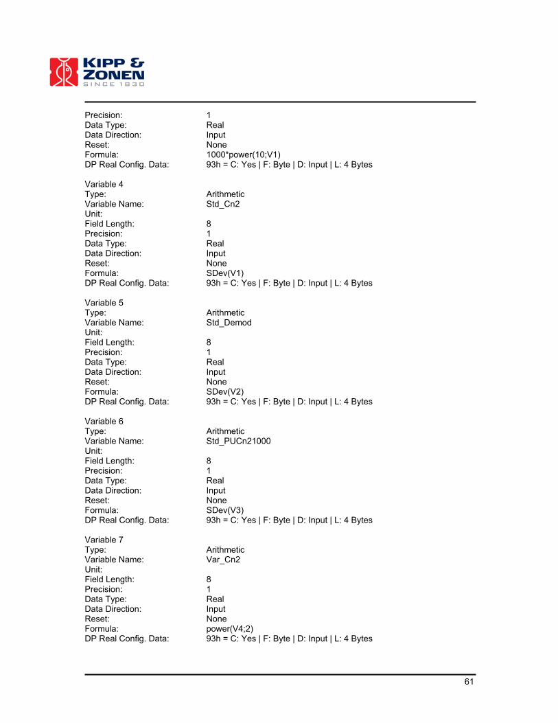
61
Precision: 1 Data Type: Real Data Direction: Input Reset: None Formula: 1000*power(10;V1) DP Real Config. Data: 93h = C: Yes | F: Byte | D: Input | L: 4 Bytes Variable 4 Type: Arithmetic Variable Name: Std_Cn2 Unit: Field Length: 8 Precision: 1 Data Type: Real Data Direction: Input Reset: None Formula: SDev(V1) DP Real Config. Data: 93h = C: Yes | F: Byte | D: Input | L: 4 Bytes Variable 5 Type: Arithmetic Variable Name: Std_Demod Unit: Field Length: 8 Precision: 1 Data Type: Real Data Direction: Input Reset: None Formula: SDev(V2) DP Real Config. Data: 93h = C: Yes | F: Byte | D: Input | L: 4 Bytes Variable 6 Type: Arithmetic Variable Name: Std_PUCn21000 Unit: Field Length: 8 Precision: 1 Data Type: Real Data Direction: Input Reset: None Formula: SDev(V3) DP Real Config. Data: 93h = C: Yes | F: Byte | D: Input | L: 4 Bytes Variable 7 Type: Arithmetic Variable Name: Var_Cn2 Unit: Field Length: 8 Precision: 1 Data Type: Real Data Direction: Input Reset: None Formula: power(V4;2) DP Real Config. Data: 93h = C: Yes | F: Byte | D: Input | L: 4 Bytes

62
Variable 8 Type: Arithmetic Variable Name: Var_Demod Unit: Field Length: 8 Precision: 1 Data Type: Real Data Direction: Input Reset: None Formula: power(V5,2) DP Real Config. Data: 93h = C: Yes | F: Byte | D: Input | L: 4 Bytes Variable 9 Type: Arithmetic Variable Name: Var_PUCn21000 Unit: Field Length: 8 Precision: 1 Data Type: Real Data Direction: Input Reset: None Formula: power(V6,2) DP Real Config. Data: 93h = C: Yes | F: Byte | D: Input | L: 4 Bytes Format output file, downloaded from COMBILOG memory: Unit, Date, Time(HH:MM:SS), UCN2, Demod, PUCN21000, Var_UCN2, Var_Demod, Var_PUCN21000, N Cn
2 can be calculated as follows (two options, see paragraph 4):
� �2
22 15.1122 10 CNUCNUnC
�����
15
2
2 10��� CNn PUC
Note: Additional measurement instructions and sensors can added to program, such as a temperature sensor, cup anemometer, pressure sensor, net radiometer and soil heat flux plates (e.g. a small micrometeorological station). Of course additional meteorological data can be taken from other nearby field stations. Note: the data file provided by the CR10X contains two Cn2 ‘formats’, which both can be read by the WINLAS software (namely, 1: UCN2 combined with Var_UCN2 , 2: PUCN2).
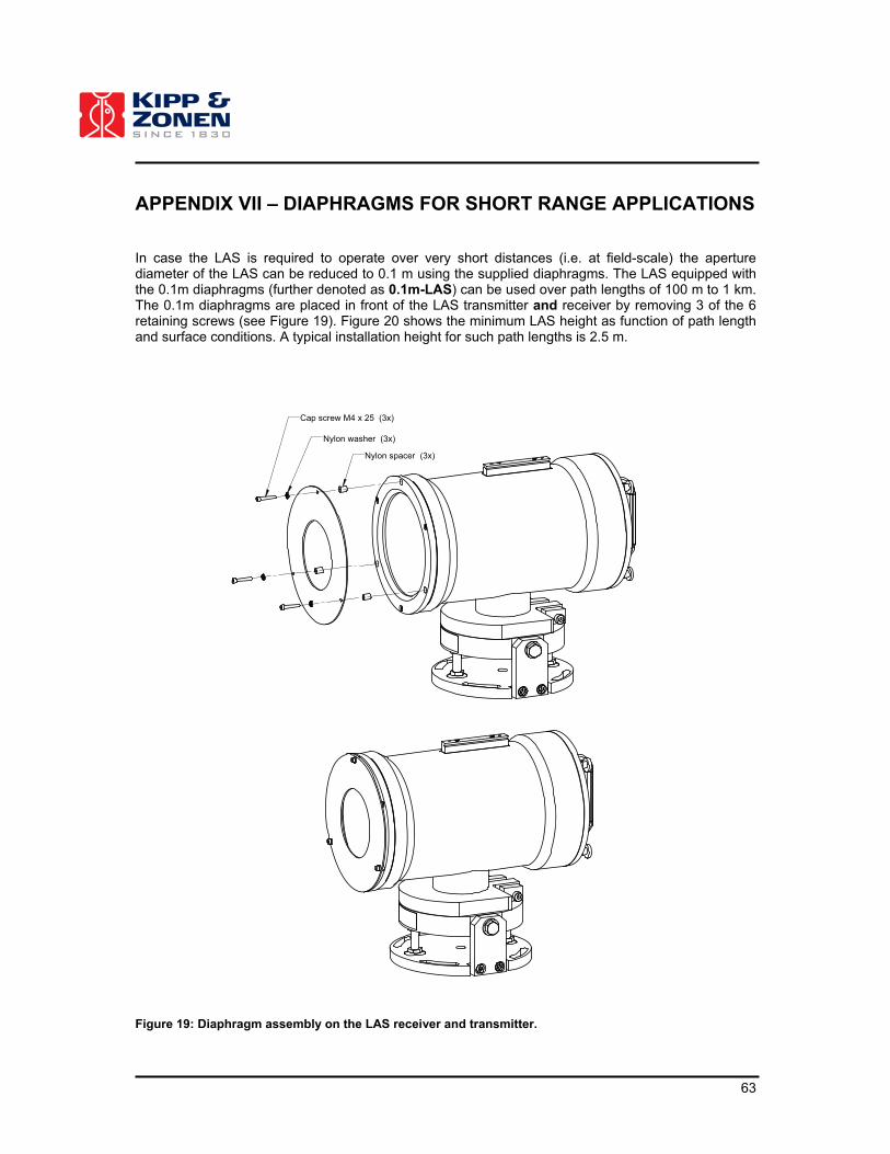
63
APPENDIX VII – DIAPHRAGMS FOR SHORT RANGE APPLICATIONS In case the LAS is required to operate over very short distances (i.e. at field-scale) the aperture diameter of the LAS can be reduced to 0.1 m using the supplied diaphragms. The LAS equipped with the 0.1m diaphragms (further denoted as 0.1m-LAS) can be used over path lengths of 100 m to 1 km. The 0.1m diaphragms are placed in front of the LAS transmitter and receiver by removing 3 of the 6 retaining screws (see Figure 19). Figure 20 shows the minimum LAS height as function of path length and surface conditions. A typical installation height for such path lengths is 2.5 m.
Cap screw M4 x 25 (3x)
Nylon washer (3x)
Nylon spacer (3x)
Figure 19: Diaphragm assembly on the LAS receiver and transmitter.
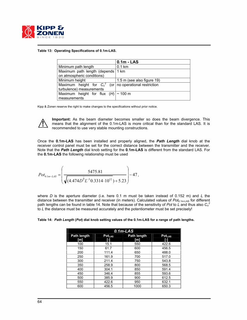
64
Table 13: Operating Specifications of 0.1m-LAS.
0.1m - LAS Minimum path length 0.1 km Maximum path length (depends on atmospheric conditions)
1 km
Minimum height 1.5 m (see also figure 19) Maximum height for Cn
2 (or turbulence) measurements
no operational restriction
Maximum height for flux (H) measurements
~ 100 m
Kipp & Zonen reserve the right to make changes to the specifications without prior notice.
Important: As the beam diameter becomes smaller so does the beam divergence. This means that the alignment of the 0.1m-LAS is more critical than for the standard LAS. It is recommended to use very stable mounting constructions.
Once the 0.1m-LAS has been installed and properly aligned, the Path Length dial knob at the receiver control panel must be set for the correct distance between the transmitter and the receiver. Note that the Path Length dial knob setting for the 0.1m-LAS is different from the standard LAS. For the 0.1m-LAS the following relationship must be used
47
23.5)103314.0474.4(
81.5475
1231.0
3
7
����
�
�
���
�
�
���
��
LDPot LASm ,
where D is the aperture diameter (i.e. here 0.1 m must be taken instead of 0.152 m) and L the distance between the transmitter and receiver (in meters). Calculated values of Pot0.1m-LAS for different path lengths can be found in table 14. Note that because of the sensitivity of Pot to L and thus also Cn
2 to L the distance must be measured accurately and the potentiometer must be set precisely!
Table 14: Path Length (Pot) dial knob setting values of the 0.1m-LAS for a range of path lengths.
0.1m-LAS Path length
[m] PotLAS
[-] Path length
[m] PotLAS
[-]
100 15.1 550 422.6 150 61.7 600 456.5 200 111.4 650 488.0 250 161.9 700 517.0 300 211.4 750 543.8 350 258.9 800 568.5 400 304.1 850 591.4 450 346.4 855 593.6 500 385.9 900 612.5 550 422.6 950 632.1 600 456.5 1000 650.3

65
Important: Data processing of the 0.1m-LAS requires WINLAS version 2.2 or higher as older versions do not support the 0.1m-LAS.
0
1
2
3
4
5
6
7
0 100 200 300 400 500 600 700 800 900 1000
path length 0.1m-LAS [m]
heig
ht
0.1
m-L
AS
[m
]
H = 50 W/m2
H = 100 W/m2
H = 150 W/m2
H = 250 W/m2
H = 300 W/m2
H = 400 W/m2 No saturation
Saturation
Figure 20: The minimum installation height of the 0.1m-LAS as function of path length and for different surface conditions. The area above the curves is the non-saturation zone. Below the curves saturation of the signal occurs. In the presence of densely packed roughness elements add the zero-displacement height (see appendix III).

66
67
APPENDIX VIII – RECALIBRATION SERVICE In order to maintain the specific performance of the LAS/XLAS instrument, Kipp & Zonen recommends calibrating the LAS/XLAS instrument when it fails the on-site calibration check (see section 7.1 and 7.2). This can be done at the Kipp & Zonen factory (see section 7.3 for a description of the procedure). Here the calibration procedure can be performed at low cost and can usually be performed within several weeks. If required, urgent calibration can be accomplished in three weeks or less (subject to scheduling restrictions). Kipp & Zonen will confirm the duration of recalibration at all times. Note that special quantity recalibration discounts are available.

68
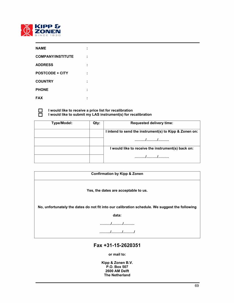
69
NAME :
COMPANY/INSTITUTE :
ADDRESS :
POSTCODE + CITY :
COUNTRY :
PHONE :
FAX :
I would like to receive a price list for recalibration I would like to submit my LAS instrument(s) for recalibration
Type/Model: Qty: Requested delivery time:
I intend to send the instrument(s) to Kipp & Zonen on:
………/………/………
I would like to receive the instrument(s) back on:
………/………/………
Confirmation by Kipp & Zonen
Yes, the dates are acceptable to us.
No, unfortunately the dates do not fit into our calibration schedule. We suggest the following
data:
………/………/………
………/………/………/
Fax +31-15-2620351
or mail to:
Kipp & Zonen B.V. P.O. Box 507 2600 AM Delft
The Netherland

70

71
Notes:

72

Our customer support remains at your disposal for any maintenance or repair, calibration, supplies and spares.
Für Servicearbeiten und Kalibrierung, Verbrauchsmaterial und Ersatzteile steht Ihnen unsere Customer Support Abteilung zur Verfügung.
Notre service 'Support Clientèle' reste à votre entière disposition pour tout problème de maintenance, réparation ou d'étalonnage ainsi que pour les accessoires et pièces de rechange.
Nuestro apoyo del cliente se queda a su disposición para cualquier mantenimiento o la reparación, la calibración, los suministros y reserva.
Passion for Precision
Go to www.kippzonen.com for your local distributor or contact your local sales office
HEAD OFFICE
Kipp & Zonen B.V.Delftechpark 36, 2628 XH Delft
P.O. Box 507, 2600 AM Delft
The Netherlands
T: +31 (0) 15 2755 210
F: +31 (0) 15 2620 351
Kipp & Zonen Asia Pacific Pte. Ltd.81 Clemenceau Avenue
#04-15/16 UE Square
Singapore 239917
T: +65 (0) 6735 5033
F: +65 (0) 6735 8019
Kipp & Zonen USA Inc.125 Wilbur Place
Bohemia
NY 11716
United States of America
T: +1 (0) 631 589 2065
F: +1 (0) 631 589 2068
Kipp & Zonen France S.A.R.L.7 Avenue Clément Ader
ZA Ponroy - Bâtiment M
94420 Le Plessis Trévise
France
T: +33 (0) 1 49 62 41 04
F: +33 (0) 1 49 62 41 02
SALES OFFICES