LARI KUMPU

EFFECTS OF USER LOCATION OPTIMIZATION IN LTE NETWORK

Master of Science Thesis

Examiners: Professor Jukka Lempiäinen

M. Sc. Joonas Säe

Examiners and topic approved by the Council

of the Faculty of Computing and Electrical

Engineering on June 4th 2014

i

ABSTRACT

TAMPERE UNIVERSITY OF TECHNOLOGY Master’s Degree Programme in Information Technology KUMPU, LARI: Effects of User Location Optimization in LTE Network Master of Science Thesis, 54 pages, 12 Appendix pages August 2014 Major: Wireless Communication Examiners: Professor Jukka Lempiäinen, M. Sc. Joonas Säe Keywords: LTE, user location, optimization

The need for developing LTE was evident as the number of users in the wireless domain

was rapidly growing and the HSDPA could not fulfill the demands in capacity set by the

users as they expected the same data rates in the wireless domain as in the wireline do-

main. Generally, user does not have an idea how much the location of itself affects the

performance of the radio network. The aim of this thesis is to demonstrate the effects of

the user location to the network and provide some insight for the user to position itself in

a way that it benefits both the operator and the user.

This thesis is divided into two parts. First part is the theory part and it consists of the

history and development of LTE and how the system targets are achieved. Basic princi-

ples of LTE network planning is described along with the propagation mechanisms and

propagation models linked with LTE. The second part is the measurements and results

with conclusions in the end. Measurements were conducted in Tietotalo of TTY in various

locations so that there are empirical results to support the conclusions. Measurement data

collected from the measurements is presented using figures and tables and conclusions

are derived from them.

As a conclusion from the results, the benefit for the user is easier to acquire, as the

user is more likely to be motivated to change their location due to the gain in performance

is on their side rather than on the operator’s side. The radio propagation environment is a

rich environment and the received signal levels change as the location of the user change.

From the results of these measurements the user should position itself in a wide and open

space and as high as possible in areas where there are no people around.

ii

TIIVISTELMÄ

TAMPEREEN TEKNILLINEN YLIOPISTO Tietotekniikan koulutusohjelma KUMPU, LARI: Effects of User Location Optimization in LTE Network Diplomityö, 54 sivua, 12 liitesivua Elokuu 2014 Pääaine: Langaton tietoliikenne Tarkastajat: Professori Jukka Lempiäinen, diplomi-insinööri Joonas Säe Avainsanat: LTE, käyttäjän sijainti, optimointi

Käyttäjien kasvavat vaatimukset langattomien verkkojen nopeuden ja kapasiteetin

suhteen olivat pohja LTE:n kehitykselle. Käytössä oleva HSDPA-teknologia ei tulisi

olemaan riittävä täyttämään nämä vaatimukset. Langattomien verkkojen tulisi kilpailla

tiedonsiirtonopeuksissa langallisten verkkojen kanssa, mihin käyttäjät olivat jo tottuneet.

Yleensä ottaen, käyttäjä ei ymmärrä kuinka paljon hänen sijaintinsa vaikuttaa verkon

toimintaan. Tämän diplomityön tarkoituksena on demonstroida kuinka paljon käyttäjän

sijainti vaikuttaa LTE-verkon suorituskykyyn ja antaa käsitys kuinka omalla

sijoittumisella voi olla hyödyksi itselleen ja operaattorille.

Diplomityö on jaettu kahteen osaan. Ensimmäinen osa on teoriaosa, jossa käsitellään

LTE:n historiaa ja kehitystä ja millä metodeilla sille asetetuille tavoitteisiin päästiin.

Tämän lisäksi käydään läpi LTE-verkon suunnittelua. Verkkosuunnittelun lisäksi

käydään läpi langattoman verkon etenemismekanismejä, monitie-etenemistä, sekä

etenemismalleja mitä käytetään LTE-teknologian yhteydessä. Toinen osuus

diplomityöstä on mittaukset ja tulokset, sekä niistä johdetut päätelmät. Mittaukset tehtiin

TTY:n tietotalossa, jotta esitetyille päätelmille olisi konkreettisia todisteita. Data, joka

kerättiin mittauksista on esitetty kuvin ja taulukoin tulososiossa, joiden perusteella

johtopäätökset on tehty.

Yhteenvetona tuloksista voi sanoa, että käyttäjän kannalta hyöty on helpommin

saavutettavissa, koska käyttäjä on motivoituneempi vaihtaa omaa sijaintia hyödyn

tullessa suoraa hänelle. Radioverkkoympäristö on rikas ja monipuolinen ympäristö ja

vastaanotetun signaalin teho vaihtelee suuresti käyttäjän sijainnin perusteella. Näiden

tulosten perusteella käyttäjän kannattaisi suosia isoja avoimia tiloja mahdollisimman

korkealla samalla välttäen muiden ihmisten liikkeistä aiheutuvaa häiriötä.

iii

PREFACE

This Master of Science Thesis is done for the Department of Electronics and Communi-

cations Engineering at Tampere University of Technology.

I would like to thank Professor Jukka Lempiäinen for providing the opportunity for this

thesis and my supervisor Joonas Säe for constant and immense support through this pro-

ject. I would also like to thank Elisa for the LTE data card that was used in the measure-

ment, Nokia for providing the LTE test network and Anite Finland for the Nemo Outdoor

and Nemo Analyze software used in the measurements.

Finally, I would like to thank my family and friends who have helped me through these

years at TUT. Without them, I would not be here.

This thesis is dedicated to my late father.

Tampere, August 13th 2014

Lari Kumpu

iv

TABLE OF CONTENTS

List of Abbreviations ..................................................................................................... vi

List of Symbols ............................................................................................................. viii

List of Figures ................................................................................................................. ix

List of Tables ................................................................................................................... x

1 Introduction ............................................................................................................. 1

2 Long Term Evolution .............................................................................................. 3

2.1 Background ....................................................................................................... 3

2.2 System Architecture Evolution (SAE) .............................................................. 4

2.2.1 User Equipment ................................................................................... 5

2.2.2 Evolved Node B ................................................................................... 5

2.2.3 Mobility Management Entity ............................................................... 6

2.2.4 Serving Gateway .................................................................................. 6

2.2.5 Packet Data Network Gateway ............................................................ 7

2.2.6 Policy and Charging Resource Function ............................................. 7

2.2.7 Home Subscription Server ................................................................... 8

2.2.8 Services Domain .................................................................................. 8

2.3 Access Methods and Modulation Schemes ....................................................... 8

2.3.1 OFDMA ............................................................................................... 9

2.3.2 SC-FDMA .......................................................................................... 11

2.3.3 MIMO ................................................................................................ 12

2.3.4 Modulation Schemes.......................................................................... 13

3 LTE Network Planning ........................................................................................ 15

3.1 Planning process ............................................................................................. 15

3.2 Nominal Planning Phase ................................................................................. 16

3.2.1 Radio Link Budget ............................................................................. 17

3.2.2 Planning Thresholds .......................................................................... 19

3.3 Detailed Planning & Optimization .................................................................. 21

4 Radio Propagation ................................................................................................ 22

4.1 Basic Propagation Mechanisms ...................................................................... 22

4.1.1 Reflection ........................................................................................... 23

4.1.2 Diffraction .......................................................................................... 23

4.1.3 Scattering ........................................................................................... 23

4.2 Multipath Fading ............................................................................................. 24

4.3 Propagation Models ........................................................................................ 24

4.3.1 The Okumura-Hata Model ................................................................. 25

4.3.2 The COST 231-Walfisch-Ikegami Model ......................................... 27

4.3.3 The COST 231 Multi-wall Model ..................................................... 30

4.3.4 The ITU Model for Indoor Attenuation ............................................. 31

5 Measurements ........................................................................................................ 33

v

5.1 Measurement Equipment and Environment .................................................... 33

5.2 Measurement Cases ......................................................................................... 34

6 Results .................................................................................................................... 37

6.1 Second Floor ................................................................................................... 37

6.2 Third Floor ...................................................................................................... 41

6.3 Fourth Floor .................................................................................................... 45

7 Conclusions ............................................................................................................ 50

References ...................................................................................................................... 53

Appendix A .................................................................................................................... 55

Appendix B .................................................................................................................... 60

vi

LIST OF ABBREVIATIONS

3G Third Generation

3GPP 3rd Generation Partnership Project

AMC Adaptive Modulation and Coding

BS Base Station

CM Cubic Metric

CP Control Plane

CQI Channel Quality Indicator

DFT Discrete Fourier Transform

DHCP Dynamic Host Configuration Protocol

eNodeB Evolved Node B

EPC Evolved Packet Core Network

EPS Evolved Packet System

E-UTRAN Evolved Universal Terrestrial Radio Network

FDMA Frequency Division Multiple Access

FFT Fast Fourier Transform

GSM Global System for Mobile Communications

HSDPA High Speed Downlink Packet Access

HSPA High Speed Packet Access

HSS Home Subscriber Server

IDFT Inverse Discrete Fourier Transform

IFFT Inverse Fast Fourier Transform

IMS IP Multimedia Subsystem

IP Internet Protocol

LOS Line-of-Sight

LTE Long Term Evolution

LTE-A LTE-Advanced

MIMO Multiple Input Multiple Output

MM Mobility Management

MME Mobility Management Entity

NLOS Non-Line-of-Sight

OFDM Orthogonal Frequency Division Multiplexing

OFDMA Orthogonal Frequency Division Multiple Access

PAPR Peak-to-Average-Peak Ratio

PAR Peak-to-Average Ratio

PCC Policy and Charging Control

PCRF Policy and Charging Resource Function

PDN Packet Data Network

P-GW Packet Data Network Gateway

vii

QAM Quadrature Amplitude Modulation

QoS Quality of Service

QPSK Quadrature Phase Shift Keying

RF Radio Frequency

RNC Radio Network Controller

RRM Radio Resource Management

SC-FDMA Single Carrier Frequency Division Multiple Access

S-GW Serving Gateway

SAE System Architecture Evolution

SINR Signal-to-Interference-plus-Noise Ratio

SNR Signal-to-Noise Ratio

SIP Session Initiation Protocol

TA Tracking Area

TUT Tampere University of Technology

UE User Equipment

UP User Plane

USIM Universal Subscriber Identity Module

viii

LIST OF SYMBOLS

∆hb Difference between building height and base station height

∆hm Difference between building height and mobile station height

σ Standard deviation

φ Angle between street orientation and incident angle

a(hm), C Area dependant factor in Okumura-Hata model

b Distance between two buildings

d Distance

f Frequency

fc Carrier frequency

hb Base station height

hm Mobile station height

hroof Building height

ka Increase of path loss if hb smaller than hroof

kd Distance related diffraction loss parameter

kf Frequency related diffraction loss parameter

kf Number of floors

kwi Number of walls of type i

Lo Free space loss

Lbsh Loss from hb being larger than hroof

Lf Loss from floors

Lmsd Multiscreen loss

Lori Street orientation correction factor

Lrts Diffraction loss

Lwi Loss from walls of type i

n Number of floors penetrated

N Power loss coefficient

PL Path loss

w Width of the street

ix

LIST OF FIGURES

Figure 2.1: Network architecture based SAE ................................................................... 4

Figure 2.2: Subcarrier spacing in OFDMA ……………………………………….……. 9

Figure 2.3: Resource allocation in OFDMA ……………………………………..……. 10

Figure 2.4: Resource allocation in SC-FDMA …............................................................ 11

Figure 2.5: Constellations of modulation schemes used in LTE ................................... 13

Figure 3.1: LTE network planning process ..................................................................... 16

Figure 3.2: Cell ranges calculated using Okumura-Hata model ….................................. 20

Figure 4.1: Basic propagation mechanisms of radio network ......................................... 22

Figure 4.2: Path losses from Okumura-Hata model in different environments .............. 26

Figure 4.3: Path losses from COST 231-Hata model in different environments ............ 27

Figure 4.4: Parameters for the COST 231-Walfisch-Ikegami model .............................. 28

Figure 4.5: Estimated path losses for COST 231-Walfisch-Ikegami model ................... 30

Figure 4.6: Estimated path losses for COST 231 Multi-wall model ............................... 31

Figure 4.7: Estimated path losses for ITU site-general model......................................... 32

Figure 5.1: Measurement points in the second floor of Tietotalo ................................... 35

Figure 5.2: Measurement points in the third floor of Tietotalo ....................................... 35

Figure 5.3: Measurement points in the fourth floor of Tietotalo...................................... 36

Figure 6.1: CDF plot of RSRP and SNR values in point 1 of the second floor ……….. 37

Figure 6.2: CDF plot of RSRP and SNR values in point 2 of the second floor .............. 38

Figure 6.3: CDF plot of RSRP and SNR values in point 5 of the second floor .............. 39

Figure 6.4: CDF plot of RSRP and SNR values in point 7 of the second floor ..……… 40

Figure 6.5: CDF plot of RSRP and SNR values in the room of the second floor ……... 41

Figure 6.6: CDF plot of RSRP and SNR values in point 1 of the third floor .................. 42

Figure 6.7: CDF plot of RSRP and SNR values in point 4 of the third floor .................. 43

Figure 6.8: CDF plot of RSRP and SNR values in point 5 of the third floor................... 44

Figure 6.9: CDF plot of RSRP and SNR values in the room of the third floor ............... 44

Figure 6.10: CDF plot of RSRP and SNR values in point 2 of the fourth floor …...….. 46

Figure 6.11: CDF plot of RSRP and SNR values in point 4 of the fourth floor …...….. 47

Figure 6.12: CDF plot of RSRP and SNR values in point 6 of the fourth floor …...….. 48

Figure 6.13: CDF plot of RSRP and SNR values in the room of the fourth floor .......... 49

x

LIST OF TABLES

Table 2.1: Theoretical data rates in downlink (Mbps) ……………………………….... 14

Table 2.2: Theoretical data rates in uplink (Mbps) ………………………………..…... 14

Table 3.1: Uplink power budget ……………………………………………………….. 18

Table 3.2: Downlink power budget ……………………………………...…………….. 19

Table 4.1: Constraints of Okumura-Hata model …………………………...………….. 25

Table 4.2: Constraints of COST 231-Walfisch-Ikegami model ……………………….. 27

Table 4.3: Used parameters for the simulation ………………………………………… 29

Table 4.4: Power loss coefficients for the ITU site-general model …………………..... 31

Table 4.5: Floor penetration losses for the ITU site-general model …………………… 32

Table 5.1: eNodeB configuration ……………………………………………………… 33

Table 5.2: Macro cell antenna specification …………………………………………… 34

Table 6.1: Calculated values of RSRP and SNR levels in point 1 of the second floor ... 37

Table 6.2: Calculated values of RSRP and SNR levels in point 2 of the second floor ... 37

Table 6.3: Calculated values of RSRP and SNR levels in point 5 of the second floor ... 39

Table 6.4: Calculated values of RSRP and SNR levels in point 7 of the second floor ... 40

Table 6.5: Calculated values of RSRP and SNR levels in the room of the second floor 41

Table 6.6: Calculated values of RSRP and SNR levels in point 1 of the third floor ....... 42

Table 6.7: Calculated values of RSRP and SNR levels in point 4 of the third floor …... 43

Table 6.8: Calculated values of RSRP and SNR levels in point 5 of the third floor …... 44

Table 6.9: Calculated values of RSRP and SNR levels in the room of the third floor ... 45

Table 6.10: Calculated values of RSRP and SNR levels in point 2 of the fourth floor .. 46

Table 6.11: Calculated values of RSRP and SNR levels in point 4 of the fourth floor .. 47

Table 6.12: Calculated values of RSRP and SNR levels in point 6 of the fourth floor .. 48

Table 6.13: Calculated values of RSRP and SNR levels in the room of the fourth floor 49

1

1 INTRODUCTION

Since the launch of Global System for Mobile Communications (GSM), the number of

mobile subscribers has increased enormously. In 2002, first billion landmark was passed,

and in 2012 it was estimated that there are more than six billion mobile subscribers in the

world, although the number of mobile subscribers is not the actual number of user pene-

tration since one user can have more than one subscription. Low-cost mobile communi-

cation has now become the preferred way of communication compared to the old landline

communication as the mobile networks cover over 90% of the world’s population. [1]

At first, GSM was designed to carry voice data only, the data capability was added

later on, and since the Third Generation (3G) networks were launched, the amount of data

traffic has hugely increased and has easily surpassed the amount of voice data. 3G net-

work introduced High Speed Downlink Packet Access (HSDPA), which enabled users to

have much higher data rates than before. HSDPA was launched in Finland in 2007 and

already in 2008, the data volume exceeded the voice data volume and in 2009, it was

already ten times larger than the voice volume. [1] As the data rates went higher, the

mobile connections were not restricted to mobile phones anymore but could be used in

laptop applications as well. With this capability, the mobile networks had soon become

packet data dominated from the previous voice data domination.

As the number of users continue to grow, so does the need for the mobile network to

evolve in order to compete with the traditional wireline technologies. Users expect to

have the same data rates in the wireless domain as in the wireline domain thus the need

of expanding the capability of wireless networks to true broadband mobile access. Wire-

less broadband access has one true advantage over wireline access and it is the ability to

provide low cost coverage to regions, where there are no existing wireline infrastructure.

Long Term Evolution (LTE) network was designed that the user data rates can match the

demands of the users.

It is natural that when the number of users grows so does the need to increase the

capacity and the coverage of the network. Mobile users are not generally aware how much

their location affects the performance of the network. The subject of this thesis is to

demonstrate what happens when the user knows how to position itself in a way that it

benefits both the network and the user. Operators can save money on deployment costs if

they plan the network correctly. If the operator can assume, that the users generally know

how to position themselves, the network can be planned cost-efficiently to fulfil the ca-

pacity and coverage requirements. At the same time, the location of the user affects the

received signal strength, which affects the upload and download speeds of the user, there-

fore is beneficial to the user to move to a better location.

2

To see the differences and benefits between the user locations, measurements are con-

ducted and from the results, general guidelines can be concluded. The situation when

taking the measurements is that the user is located within a building and the signal is

coming from outdoors. This is the most common case when using mobile phones and the

network planning is more difficult when taking into account the indoor coverage of the

cell.

3

2 LONG TERM EVOLUTION

To develop a new radio network technology it takes years from the beginning of the re-

search to the commercial launch of the network. This chapter governs the basic principles,

which enabled LTE to fulfil the requirements set for it.

2.1 Background

The work for LTE started few years before HSDPA was even deployed in 2004 as it takes

more than five years from the start of the project to the commercial launch. It was obvious

that when the wireline technologies improve so should the wireless domain also. The need

for wireless capacity was greatly increased as HSDPA was launched thus LTE was sup-

posed to meet the demands and it should be able to compete with other wireless technol-

ogies. [1]

As in any 3rd Generation Partnership Project (3GPP) project, the development of LTE

started with setting the system targets. LTE should deliver superior performance to any

other network, which uses High Speed Packet Access (HSPA) technology by optimally

using available spectrum and base station sites. Spectral efficiency should be at least two

to four times greater than with the HSPA Release 6. Peak data rates should be at least 100

Mbps and 50 Mbps in downlink and uplink direction. With the faster data rates, the sys-

tem latency should be dropped and the target set here was that the round trip time should

be less than 10 milliseconds and access delay less than 300 milliseconds. Terminal power

consumption has to be optimized, so that it would be more feasible to use multimedia

applications without recharging the battery all the time. The network should be packet

switched optimized with high level of mobility and security and when planning the net-

work the frequency allocation should be flexible. [2]

To meet the set data rate targets LTE uses Orthogonal Frequency Division Multiple

Access (OFDMA) in the downlink and Single Carrier Frequency Division Multiple Ac-

cess (SC-FDMA) in the uplink. Orthogonality in these techniques provides less interfer-

ence between users and more capacity. Resources are divided in the frequency domain,

which is the main reason for the high capacity of LTE. Closer look on the modulation

techniques is taken in chapter 2.3. Due to flexible spectrum allocation, the transmission

bandwidth can be between 1.4 MHz and 20 MHz, which enables data rates in downlink

up to 150 Mbps using 2 x 2 Multiple Input Multiple Output (MIMO) antenna configura-

tion and 300 Mbps using 4 x 4 MIMO configuration. In uplink, the peak data rate is 75

Mbps when using 2 x 2 MIMO. [2]

To reduce the round trip time and the access delay, the network architecture is sim-

plified in LTE compared to the previously released technologies. What used to be tasks

4

for the Radio Network Controller (RNC) is now placed in the base stations. What started

as a workgroup in 2004, the protocol was frozen in 2009, and the first commercial net-

works were launched in 2010. [1]

2.2 System Architecture Evolution (SAE)

As was mentioned in the previous chapter, simpler system architecture was needed to

reduce the delays caused by different components of the network and to enable faster data

rates. Circuit switched elements could now be removed as LTE only relies on the packet

switched network. This flat architecture uses fewer nodes in the network, which directly

causes less delay. This on the other hand results that the used nodes would have to be

more complex to ensure that the network works as it should and also with other 3GPP

and wireless access networks. [1]

This newly designed architecture consists of User Equipment (UE), Evolved Univer-

sal Terrestrial Radio Access Network (E-UTRAN), Evolved Packet Core (EPC) and the

Services Domain and it is described in Figure 2.1.

Figure 2.1. Network architecture based on SAE [1 p. 25].

5

The first three elements now form the Internet Protocol (IP) Connectivity Layer or the

Evolved Packet System (EPS). The main task of this layer is to provide IP connectivity

into and out of the network. Since the circuit switching is now removed, the layer is op-

timized only for the packet switching. Transportation and services are now on top of IP.

[1]

E-UTRAN is a mesh of evolved Node Bs (eNodeB). These improved base stations

now handle all the radio functionality of the network and they serve as a termination point

of all radio related protocols. eNodeBs are connected to each other with the X2 interface

to form the network. [1]

EPC is equivalent to the packet switched domain of the previous 3GPP networks but

there are major functionality changes in it. It forms the connection between E-UTRAN

and the Services Domain through two elements: the Serving Gateway (S-GW) and the

Packet Data Network Gateway (P-GW). EPC also contains the Mobility Management

Entity (MME), which handles the main control elements of the EPC. [1]

2.2.1 User Equipment

User equipment, like in the legacy 3GPP technologies, is now the device, which the end

user uses. It can be a handheld mobile device or a laptop containing the Universal Sub-

scriber Identity Module (USIM), which identifies and authenticates the user and enables

the decryption of radio interface transmissions. The main tasks of the UE are setting up

and maintaining connections to the eNodeBs, location updates and handovers as in-

structed by the network, and finally providing the user interface for the user applications

of the UE. [3]

2.2.2 Evolved Node B

The only node in E-UTRAN is now the eNodeB. It serves as a layer 2 gateway between

the UE and the EPC. These Base Stations (BS) are placed near the actual antenna config-

urations, serve as a termination point of all radio protocols towards the UE, and forward

the data between radio protocol and IP connectivity to the EPC. eNodeB ciphers and de-

ciphers data in the User Plane (UP) and compresses the IP headers so that the data does

not have to be sent unnecessarily, which has a straight impact on the available capacity

of the network. [3]

Apart from the UP functions, eNodeBs are also responsible for the functionality of

the Control Plane (CP). Important functionality of the eNodeBs is that they are responsi-

ble for the Radio Resource Management (RRM), which was before the responsibility of

the RNC in the 3G networks. RRM functions handle the allocation and monitoring of the

available resources according to the Quality of Service (QoS). [3]

Mobility Management (MM) is also a part of eNodeBs duties. eNodeB constantly

receives measurements made by the UE of the radio signal levels, makes similar meas-

6

urements itself, and decides if handovers are needed based on those results. If the hando-

ver is made the eNodeB is also responsible for exchanging signalling information to other

eNodeBs and MMEs. At any time, the UE is connected to only one eNodeB, but the

eNodeB can be connected to a multiple UEs and other eNodeBs and MMEs. The other

connected eNodeBs are those to which the handover can be made. [3]

As the eNodeB can be connected to multiple MMEs and S-GWs the UE can be served

by one of each so the eNodeB has to keep track which UE is connected to which of these

elements.

2.2.3 Mobility Management Entity

MME is the main element in the EPC, which is responsible for the CP data handling. The

User Plane information exchange is completely left out of MMEs duties and it is directly

connected to the UE. One of the main tasks of the MME is the authentication of the UE

and securing the transmissions of the UE. When the UE first registers to a MME, the

MME starts the authentication procedure by requesting the permanent ID of the UE from

the UE itself or the previously visited network. Then the authentication vector is requested

from the UE’s Home Subscription Server (HSS), which is then compared to the authen-

tication vector received from the UE. If they match then the UE is verified. [3]

Second task of the MME is the mobility management. MME tracks all the UEs in its

service area. When a UE first registers to a MME, it forwards the location of the UE to

the HSS of its home network and then allocates resources from the eNodeB and an S-GW

for it. Resource allocation is based on the activity mode changes. Location updates are

received from the eNodeB if the UE is connected to it or from the Tracking Area (TA) if

the UE is in idle mode that is, it is not in active communication with an eNodeB. A track-

ing area is a set of eNodeBs, which are connected to a MME. In the case of handover, the

MME handles signalling between eNodeBs, S-GWs and other MMEs. [3]

When a UE registers to a MME it retrieves the UEs subscription profile from the UE’s

home network and therefore determines which Packet Data Network connections should

be allocated to it. MME always allocates a basic IP connectivity but later on it can prior-

itize connections by setting up dedicated bearers from the S-GW or from the UE based

on the requests made by operator service domain or the UE. [3]

As mentioned before, a MME can be connected to a multiple MMEs, eNodeBs, S-

GWs and UEs. This causes more complex solutions in the MMEs but reduces the overall

complexity of the network architecture.

2.2.4 Serving Gateway

Serving Gateways maintain the tunnel management and switching in the UP domain. The

main task is handling the GPRS Tunnelling Protocol tunnels in the UP interfaces and

control requests come from the MME to the P-GW. S-GWs are little involved in other

control functions and allocate resources only for themselves. Allocation requests come

again from other logical units of the network that is the MME, the P-GW or the Policy

7

and Charging Resource Function (PCRF) unit. These units are used to set up, clear and

modify bearers for a UE. [3]

During handovers, S-GW acts as an anchor point and tunnels data and resources from

the source eNodeB to the target eNodeB. If a UE is in connected mode, S-GWs tunnel

the data between the serving eNodeB and the P-GW. In the case of data coming from the

P-GW and the serving tunnel is terminated, the S-GW buffers the data and informs the

MME to start paging the UE for which the data belongs. S-GW also collect and monitor

data for accounting, user charging and relaying monitored data to authorities for further

inspection. [3]

From S-GW point of view, it is connected to multiple MMEs and eNodeBs in its

control area and has to be able to connect to any P-GW in the network. Connections to

the UE are on the other hand always handled through only one MME and eNodeB.

2.2.5 Packet Data Network Gateway

Packet Data Network Gateway is the edge router between the EPS and the external packet

network. P-GWs are the IP attachment points for UEs and allocate them with an IP ad-

dress using the Dynamic Host Configuration Protocol (DHCP) from internal or external

servers. This is done automatically when UE requests a Packet Data Network (PDN) con-

nection and the address can be IPv4 or IPv6, or both if needed. [3]

As the P-GW is the edge router between networks, all the data in the UP and between

the P-GW and the external network is in the form of IP packets. Depending on the con-

figuration of interfaces between the logical nodes of the network, P-GWs set up the tun-

nelling between the external network and the PCRF node or the MME. During handovers,

that is when the S-GW changes, the P-GW is responsible for setting up new bearers after

getting confirmation from the new S-GW. P-GWs also collect and monitor traffic in the

same fashion as the S-GWs. [3]

P-GW behaves in a similar way as other logical nodes of the network. It is connected

to several other logical nodes and external networks, but when connected to a UE, it is

served through only one S-GW.

2.2.6 Policy and Charging Resource Function

Policy and Charging Resource Function is the logical unit in the network, which is re-

sponsible for the Policy and Charging Control (PCC). It monitors the QoS of the services

and provides information of them to the P-GWs, and information of setting up bearers is

sent to the S-GWs. PCC rules are provided upon requests, which come from P-GWs, S-

GWs or from the Services Domain in the case of the UE directly signalling with the Ser-

vices Domain. Bearer allocation is done initially when the UE connects to a network or

when dedicated bearers are needed. PCRFs are also associated with several other nodes

in the network but only one PCRF is associated by every PDN connection the UE has. [3]

8

2.2.7 Home Subscription Server

Home Subscription Server is the place where all the permanent user data is stored. It

keeps track of the subscribers, which are located in its service area and knows their loca-

tion on the level of which MME they use. HSS has information about services, which

each subscriber is allowed to use and the encryption keys of the users, which are requested

upon authentication of users when connecting to a new network. In signalling, the HSS

interacts with the MME and maintains connections based on information gained from the

MMEs about UEs they serve. [3]

2.2.8 Services Domain

The Architecture of the Services Domain is not strictly defined and the services it pro-

vides depends on the operator. IP Multimedia Subsystem (IMS) has its own definition in

the standards and it provides services using the Session Initiation Protocol (SIP). Other

services depend on the operator or they are gained through the Internet for example. [3]

2.3 Access Methods and Modulation Schemes

One major aspect to reach high data rates was the use of multicarrier modulation tech-

niques. In the legacy systems, a single carrier was used and by adjusting the phase or the

amplitude, or both, symbols were accordingly transmitted. Frequency could also be ad-

justed, but in LTE, it does not affect the modulation. By increasing the data rate also the

symbol rate would have to be increased which resulted in higher bandwidth since there is

no overlap between the carriers transmitted. By using the Quadrature Amplitude Modu-

lation (QAM) the phase and amplitude of the carrier is adjusted to carry a different num-

ber of bits. The higher the order of QAM, the higher the number of bits carried. [1]

The single carrier method is not spectrally efficient, hence a better method had to be

used. Frequency Division Multiple Access (FDMA) method divides the available band-

width equally into subcarriers, which different users can utilize, or they could just use

different carriers. Subcarrier spacing should be chosen in way that they do not interfere

with each other and unnecessary guard bands would be obsolete. Orthogonal Frequency

Division Multiple Access (OFDMA) was the key to solve these problems. OFDMA uses

constant spacing between the overlapping subcarriers but the waveforms of the subcarri-

ers do not cause interference with the neighbouring subcarriers. At each sampling instant,

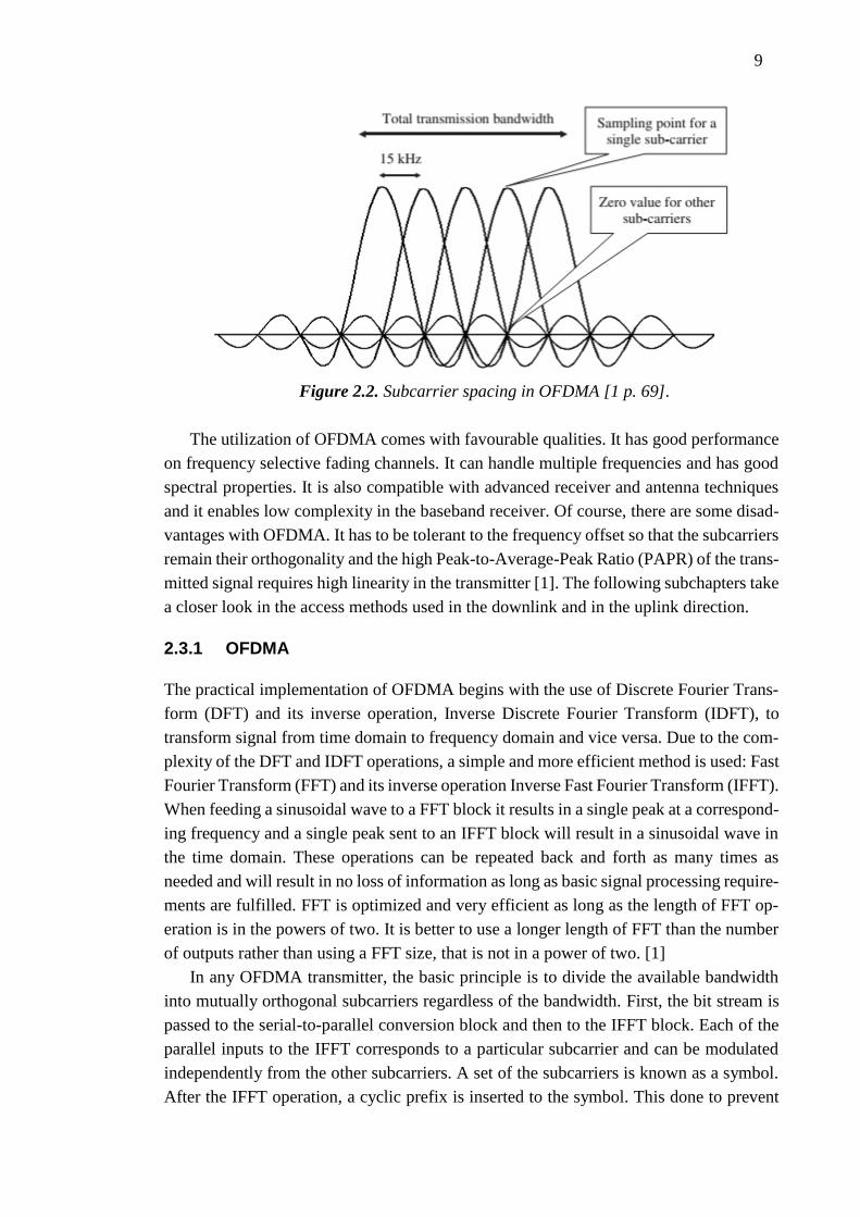
all but one subcarrier has zero value. In LTE, this subcarrier spacing is 15 kHz, which

can be seen from Figure 2.2. LTE uses this modulation method in the downlink and many

of the aspects in the uplink. [1]

9

Figure 2.2. Subcarrier spacing in OFDMA [1 p. 69].

The utilization of OFDMA comes with favourable qualities. It has good performance

on frequency selective fading channels. It can handle multiple frequencies and has good

spectral properties. It is also compatible with advanced receiver and antenna techniques

and it enables low complexity in the baseband receiver. Of course, there are some disad-

vantages with OFDMA. It has to be tolerant to the frequency offset so that the subcarriers

remain their orthogonality and the high Peak-to-Average-Peak Ratio (PAPR) of the trans-

mitted signal requires high linearity in the transmitter [1]. The following subchapters take

a closer look in the access methods used in the downlink and in the uplink direction.

2.3.1 OFDMA

The practical implementation of OFDMA begins with the use of Discrete Fourier Trans-

form (DFT) and its inverse operation, Inverse Discrete Fourier Transform (IDFT), to

transform signal from time domain to frequency domain and vice versa. Due to the com-

plexity of the DFT and IDFT operations, a simple and more efficient method is used: Fast

Fourier Transform (FFT) and its inverse operation Inverse Fast Fourier Transform (IFFT).

When feeding a sinusoidal wave to a FFT block it results in a single peak at a correspond-

ing frequency and a single peak sent to an IFFT block will result in a sinusoidal wave in

the time domain. These operations can be repeated back and forth as many times as

needed and will result in no loss of information as long as basic signal processing require-

ments are fulfilled. FFT is optimized and very efficient as long as the length of FFT op-

eration is in the powers of two. It is better to use a longer length of FFT than the number

of outputs rather than using a FFT size, that is not in a power of two. [1]

In any OFDMA transmitter, the basic principle is to divide the available bandwidth

into mutually orthogonal subcarriers regardless of the bandwidth. First, the bit stream is

passed to the serial-to-parallel conversion block and then to the IFFT block. Each of the

parallel inputs to the IFFT corresponds to a particular subcarrier and can be modulated

independently from the other subcarriers. A set of the subcarriers is known as a symbol.

After the IFFT operation, a cyclic prefix is inserted to the symbol. This done to prevent

10

the inter-symbol interference and it has to be longer than the channel impulse response.

The prefix is a part of the signal in the end, which is added to the beginning of the symbol.

However, this causes the symbol to appear as a periodic signal and the impact of the

channel corresponds to a multiplication of the signal by a scalar. The periodic nature of

the signal also enables the use of FFT and IFFT. The length of the cyclic prefix has to be

longer than the delay spread of the channel and the filtering needs of the transmitter and

receiver has to be taken into account. [1]

The wireless channel usually causes amplitude and phase shifts to individual subcar-

riers, which the receiver must be able to deal with. This is done by transmitting pilot

symbols. Reasonably chosen in time and frequency domain these pilot symbols are inter-

preted in the receiver, which can revert the effects on the subcarriers caused by the chan-

nel. Usually this is done with frequency domain equalizer. Pilot placement has to take

into account also in the neighbouring cells and when using multiple antennas. [1]

Other tasks of receiver are the time and frequency synchronizations. This has to be

done so that the correct symbol and correct part of the symbol is obtained. Correct part of

the symbol is easier to get just by comparing the known data in example pilot symbol

with the received data. Frequency synchronization estimates the frequency offset from

the transmitter to the receiver and it has to be done with great accuracy or it can render

the symbol useless. With a good estimate of the offset, it can be compensated in both the

transmitter and the receiver. [1]

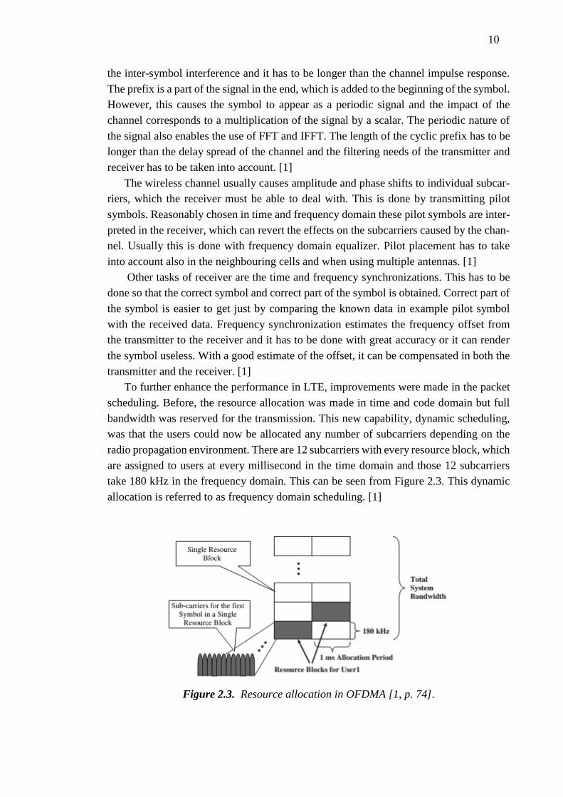
To further enhance the performance in LTE, improvements were made in the packet

scheduling. Before, the resource allocation was made in time and code domain but full

bandwidth was reserved for the transmission. This new capability, dynamic scheduling,

was that the users could now be allocated any number of subcarriers depending on the

radio propagation environment. There are 12 subcarriers with every resource block, which

are assigned to users at every millisecond in the time domain and those 12 subcarriers

take 180 kHz in the frequency domain. This can be seen from Figure 2.3. This dynamic

allocation is referred to as frequency domain scheduling. [1]

Figure 2.3. Resource allocation in OFDMA [1, p. 74].

11

Because of these subcarriers corresponds in the time domain as multiple sinusoidal

waves with different frequencies, it makes the signal envelope vary rapidly. This is a

challenge especially for the amplifier whose objective is to get maximal amplification

with the minimal power consumption. The amplifiers must use a back off to stay in the

linear region of the amplifier, which is now larger than when using a single carrier signal.

This back off now results in reduced amplification or output power, which then causes

the uplink range to be shorter or in increased power consumption. This was the main

reason LTE uses OFDMA in the downlink and SC-FDMA in the uplink. [1]

2.3.2 SC-FDMA

Where the single carrier aspect in SC-FDMA could be seen as QAM modulation in the

time domain, where each symbol is sent one at a time, OFDMA principle is added to

facilitate the resource allocation in the frequency domain also. As in the downlink, the

need for cyclic prefixes is also here. This time the prefixes are added between the block

of symbols as the symbol rate is faster than in OFDMA. The receiver still needs to deal

with the inter-symbol interference between the cyclic prefixes and this is done with equal-

izer running through the resource block until reaching the cyclic prefix. [1]

Users are allocated continuous part of the frequency bandwidth, which is occurring at

one millisecond intervals. When the frequency domain resource allocation is doubled, the

data rate doubles thus making the individual transmission shorter in time but wider in the

frequency domain. In practice this is not the case though, cyclic prefixes and guard bands

take away some of the system bandwidth available, resulting in smaller usable transmis-

sion bandwidth. [1]

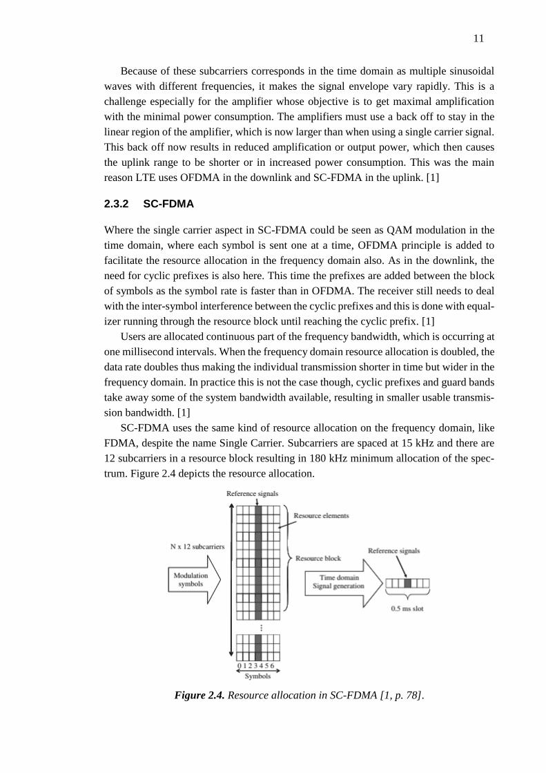
SC-FDMA uses the same kind of resource allocation on the frequency domain, like

FDMA, despite the name Single Carrier. Subcarriers are spaced at 15 kHz and there are

12 subcarriers in a resource block resulting in 180 kHz minimum allocation of the spec-

trum. Figure 2.4 depicts the resource allocation.

Figure 2.4. Resource allocation in SC-FDMA [1, p. 78].

12

After the resources are mapped, the signal is fed into a time domain signal generator

to generate the SC-FDMA signal. Every subcarrier has a reference signal, which is used

for the channel estimation in the receiver. [1]

Since the different users are sharing the resources in the frequency domain, the base

station needs to keep track and control each of the transmissions. This is done by modi-

fying the IFFT block in the transmitter. Transmissions from different users can be placed

at their own part of the spectrum. The receiver in the base station knows which users

transmission is on which resource block, since the uplink utilization is based on the base

station scheduling. [1]

OFDMA systems have trouble with the signal envelope because of the multiple si-

nusoidal waves of each subcarrier. In SC-FDMA; only one modulated symbol is trans-

mitted at a time in the time domain, the system is able to keep its good envelope proper-

ties, and the waveform properties are gained from the modulation method used. This al-

lows the SC-FDMA to obtain a very low Peak-to-Average Ratio (PAR) and Cubic Metric

(CM), which is specially used in describing the impact of the amplifier. Low CM allows

the amplifier to operate at the maximum power level with the minimum back off. This

enables good power conversion efficiency and low power consumption. [1]

Since there are cyclic prefixes only after a block of symbols, it causes extra complex-

ity and processing power in the base stations. However, it was decided, that the overall

benefits exceed those disadvantages. The benefit from the dynamic allocation of re-

sources removed the need for baseband receiver on standby in the UE, but the base station

receiver is used for those users, who have data to transmit. [1]

2.3.3 MIMO

Major contribution in increasing the data rates comes from the use of multiple antennas

including spatial multiplexing, pre-coding and transmit diversity. This was introduced in

the first release of LTE [4]. Increase of the peak data rate by a factor of two or even by

four comes simply from using two or four antennas, respectively. These antennas in the

transmitting end are fed with different data streams and in the receiver, these data streams

are separated hence increasing the data rate. Pre-coding benefits the transmission by

weighting the transmitted signals to maximize the SNR. Transmit diversity on the other

hand uses multiple antennas to transmit the same signal to benefit from the different signal

propagation paths they propagate through. In order to maximize the benefit of MIMO, a

high SNR is required and OFDMA system is well suited for this. [1]

To achieve separation between transmitting antennas and their data streams, reference

symbol mapping is needed. One antenna uses some resource blocks as reference symbols,

which are left unused by the second antenna. This can be applied to even more antennas

but results in reference symbol overhead and more complex solutions on the receiver and

transmitter design. [1]

The uplink direction in LTE also supports the use of MIMO. However, the single user

data rate cannot be doubled, because the devices use only one antenna to transmit. The

13

cell level data rate can be doubled by allocating two users with orthogonal reference sig-

nals in the same frequency resource block. The base station treats this transmission as a

MIMO transmission and therefore doubling the data rate. From the device’s point of view,

this does not require systems that are more complex but in the base station, additional

processing is needed for the user separation. SC-FDMA enables high local SNR, which

is one of the MIMO operation requirements. [1]

2.3.4 Modulation Schemes

LTE uses three different modulation schemes for the user data in the uplink and downlink

direction. Modulation used are Quadrature Phase Shift Keying (QPSK), 16-QAM and 64-

QAM, although the use of 64-QAM in the uplink direction is dependant of the UE’s ca-

pability. Modulation schemes can carry different number of bits, those being two, four

and six respectively [1]. Constellations of the modulation schemes can be seen from Fig-

ure 2.5.

Figure 2.5. Constellations of modulation schemes used in LTE [1, p. 85].

The actual modulation used depends on the signal level received at the UE. 64-QAM

enables the highest data rates but it requires higher signal levels i.e. 64-QAM can only be

used near the base station and has the lowest coverage. QPSK has the biggest coverage

and it is used near the cell edge when the transmit power is at its maximum, leaving the

16-QAM used between these zones. LTE uses adaptive modulation and coding (AMC) to

switch between the modulation schemes and coding rates depending on the received SNR

[1]. Therefore the SNR affects the data rates in achieved by the user.

Table 2.1 and Table 2.2 show the theoretical maximum data rates associated with each

modulation scheme, bandwidth and MIMO usage [1].

14

Table 2.1. Theoretical data rates in downlink (Mbps).

Bandwidth 1.4 MHz 3 MHz 5 MHz 10 MHz 15 MHz 20 MHz

Resource Blocks 6 15 25 50 75 100

Modulation

QPSK 0.9 2.3 4.0 8.0 11.8 15.8

16-QAM 1.8 4.6 7.7 15.3 22.9 30.6

64-QAM 4.4 11.1 18.3 36.7 55.1 75.4

64-QAM (2x2 MIMO) 8.8 22.2 36.7 73.7 110.1 149.8

Table 2.2. Theoretical data rates in uplink (Mbps).

Bandwidth 1.4 MHz 3 MHz 5 MHz 10 MHz 15 MHz 20 MHz

Resource Blocks 6 15 25 50 75 100

Modulation

QPSK 1.0 2.7 4.4 8.8 13.0 17.6

16-QAM 3.0 7.5 12.6 25.5 37.9 51.0

64-QAM 4.4 11.1 18.3 36.7 55.1 75.4

Data rates are calculated in a way that transport block sizes are taken into considera-

tion so that uncoded transmission is not possible. Target data rates set for LTE was 100

Mbps in downlink and 50 Mbps in uplink so they are clearly met using these methods.

15

3 LTE NETWORK PLANNING

Planning a radio network is a complicated process and it takes a lot of effort to design and

implement a working network. This chapter goes through what is done in the planning

phase with the focus on the radio link budget, which is probably the most important tool

in the planning.

3.1 Planning process

Network planning in LTE happens in a same way as it is done in the legacy systems and

is carried out in three phases. The first phase is the nominal planning phase, where the

number of eNodeBs is estimated to provide a sufficiently high quality service for each

cluster. The clusters represent the radio propagation environment such as dense urban,

urban, suburban and rural areas. Estimate of the required base stations per cluster type

can be calculated using the link budget. [5]

Detailed planning phase is done site-by-site basis in which each site is tuned to the

specific propagation environment as it naturally differs from site to site. Antenna direc-

tions, down tilting and power levels are modified according to propagation models and

planning software. Field measurements and topology maps are used to tune the propaga-

tion models and help predict the local coverage areas. [5]

The last phase is the optimization phase. Usually it is done before and after the initial

launch of the network and can last until the end of the lifecycle of the LTE network.

Capacity and QoS requirements change throughout the life of the network and operators

need to keep up with them. Field tests are made to investigate the user profiles and data

is collected to see data usage, performance figures and possible faults. [5]

Depending on the operator’s position in the market, the number of existing sites from

the 2G/3G systems affects the planning of the LTE network. It is essential to reuse exist-

ing sites to keep the deployment costs minimal. At first, the coverage of the LTE network

is minimal and provides only hotspots for the system but as the technology matures the

coverage increases also due to the competition between other operators. As the LTE net-

work starts to grow, the operator can gradually reduce the capacity of the older systems,

which then frees up bandwidth and can be refarmed to the LTE network. [5]

For greenfield operators, the benefit is that the LTE network is planned optimally

right from the beginning due to no constraints from the previous systems but the disad-

vantage is that the deployment is more expensive. Site hunting must be made early in the

planning process and there must be a constant feedback loop between the planning pro-

cess and site hunting as the latter does not provide optimal site locations. In addition,

there must be at least some planning in the transmission and core network together with

the site hunting. [5]

16

Figure 3.1. LTE network planning process [5 p. 260].

Figure 3.1 shows the main phases of the planning process. The next chapters focus on

the dimensioning phase of the planning and describing the main ideas of the last two

phases.

3.2 Nominal Planning Phase

Nominal planning phase is often referred to as dimensioning. As previously mentioned

the target is to get an estimate of the network infrastructure under the current area con-

sidered, required level of QoS and estimated traffic capacity. Simpler models are used in

the dimensioning than in detailed planning but the inputs for the dimensioning must be

with an acceptable level of accuracy; otherwise estimates may provide false results.

These inputs include the number of subscribers in the area and its geographical type,

traffic distribution, frequency band used, available bandwidth and coverage and capacity

requirements. Generally, the dimensioning happens in the same way in any wireless tech-

nology but there are system specific parameters, which affect the radio link budget di-

rectly. Propagation models are used to calculate the cell range and the models used depend

on the frequency of the system as well as the propagation environment. These are covered

more in the next chapter.

In LTE, the dimensioning inputs are broadly divided to quality, coverage and capacity

related inputs. Quality related inputs are average cell throughput and blocking probability.

17

These parameters are used to estimate the level of quality the service provides its users.

In addition, the cell edge performance can be used in the dimensioning tool to calculate

the cell radius and therefore the number of sites. [6]

The most important tool in the coverage planning is the radio link budget. The radio

link budget includes gains and losses from the transmitting and receiving end, cell loading

and propagation models. In addition, the channel type and geographical information is

used in coverage dimensioning and the coverage probability affects the cell radius calcu-

lation. Radio link budget is covered more thoroughly in the next section. [6]

Capacity planning inputs are the number of subscribers in the area, their demanded

services and the level of usage. The available spectrum and bandwidth play a vital role in

the planning process. The number of supported users per cell is determined based on the

traffic analysis and data rates needed to support the available services. The number of

users a single cell supports therefore calculates the number of cells needed. [6]

As mentioned the output of the dimensioning process is the estimate of the number of

eNodeBs. Two values of the cell radii are gained from the dimensioning. First value is

from the coverage planning and second from the capacity planning. The smaller of these

two is used in to calculate the area one cell provides which can be then used to calculate

the number of sites the planned area requires. [6]

3.2.1 Radio Link Budget

Using the link budget, the network designers can estimate the maximum signal attenua-

tion between the mobile and the base station. With this path loss, maximum cell range

can be calculated using a suitable propagation model such as Okumura-Hata. From the

cell range, the area covered by the site can be calculated and from there, the number of

sites needed to cover the planned area.

The LTE link budget does not differ much from the WCDMA link budget so it is

added for comparison in Table 3.1 and Table 3.2. For this reason, it is easier for the de-

signer to see how well the new LTE network will perform when deployed in the existing

sites of WCDMA. Table 3.1 is an example of an uplink power budget, Table 3.2 is a

downlink power budget and the parameters used are described next.

The maximum transmit power of a UE depends on the power class of a UE. In this

case it is the transmit power of a class 3 and it can be reduced depending on the modula-

tion used. Typically, the antenna gain of a UE is set to zero but in some cases, it can even

be negative or up to 10 dBi if the terminal has a directive antenna. Body loss is used in

voice link budgets, as in this budget, but otherwise set to zero. Effective Isotropic Radi-

ated Power (EIRP) is calculated by subtracting the losses and adding the gains of the UE

with the transmit power. EIRP is the radiated power of the antenna to a single direction.

[1]

In the receiving end is the eNodeB. The noise figure in the eNodeB has to be 5 dB at

maximum but actual noise figure depends on the implementation and it is usually lower.

Thermal noise is the noise generated by the components in the equipment and depends

18

on the bandwidth used and the temperature of the operating device. In this case, the band-

width is equal to two resource blocks resulting in 360 kHz and operating at temperature

of 290 K. The used bandwidth depends on the bit rate used, which is low in this case.

Receiver noise is the amount of noise caused by the receiving equipment. Signal to inter-

ference plus noise ratio (SINR) is the ratio between the received signal power and the

sum of noise and interference. SINR value depends on the modulation and coding

schemes, which are dependent on the data rate and resource blocks used. Receiver sensi-

tivity is the minimum level of a signal, which the receiver can observe. It is calculated by

adding the SINR and receiver noise together. [1]

Interference margin is the interference caused by other cell users since the users in the

same cell are orthogonal with each other. As the cell load increases due to increase of the

users, so does the interference margin. With the increase of the interference margin, the

coverage of the cell decreases. This effect is called cell breathing and it is lower in LTE

than in the previous systems. Cable loss between the low noise amplifier and the base

station depend on the cable length and type and the frequency used. The gain of the an-

tenna depends on the antenna size and the number of antenna elements used. Fast fading

and soft handover gains are not used in LTE [1].

Maximum path loss can be then calculated by adding and subtracting the thermal

noise, losses and gains of the receiver with the EIRP value. As can be seen from the table,

the values of LTE and HSPA path losses do not differ much from each other.

Table 3.1. Uplink power budget.

Variable HSPA LTE Equation

Data rate (kbps) 64 64

Transmitter–UE

a Max TX power (dBm) 23 23

b TX antenna gain 0 0

c Body loss (dB) 3 3

d EIRP (dBm) 20 20 d = a - b - c

Receiver–(e)Node B

e (e)NodeB noise figure (dB) 2 2

f Thermal noise (dB) -108.2 -118.4

g Receiver noise (dBm) -106.2 -116.4 g = e + f

h SINR (dB) -17.3 -7

i Receiver sensitivity (dBm) -123.5 -123.4 i = g + h

j Interference margin (dB) 3 1

k Cable loss (dB) 0 0

l RX antenna gain (dBi) 18 18

m Fast fade margin (dB) 1.8 0

n Soft handover gain (dB) 2 0

o Maximum path loss 158.7 160.4 o = d - i - j - k + l - m + n

19

Table 3.2. Downlink power budget.

Variable HSPA LTE Equation

Data rate (kbps) 1024 1024

Transmitter–(e)Node B

a TX power (dBm) 46 46

b TX antenna gain (dBi) 18 18

c Cable loss (dB) 2 2

d EIRP (dBm) 62 62 d = a + b - c

Receiver–UE

e UE noise figure (dB) 7 7

f Thermal noise (dB) -108.2 -104.5

g Receiver noise floor (dBm) -101.2 -97.5 g = e + f

h SINR (dB) -5.2 -9

i Receiver sensitivity (dBm) -106.4 -106.5 i = g + h

j Interference margin (dB) 4 4

k Control channel overhead (dB) 0.8 0.8

l RX antenna gain (dB) 0 0

m Maximum path loss 163.6 163.7 m = d - i - j - k + l

In the downlink power budget the transmitter is eNodeB and the receiver is a UE. Natu-

rally the downlink link budget is similar to the uplink link budget and the biggest differ-

ences in the transmitting end is the EIRP of the base station antenna as the antenna has

larger gain and more transmit power. In the receiving end, the UE has bigger noise figure

due to space limitation of the UE, therefore the quality of components is reduced. Thermal

noise is bigger, as the number of resource blocks is increased to provide higher data rate.

Control channel overhead is the loss caused by reference signals in the control channels.

[1]

3.2.2 Planning Thresholds

Previous link budget is the general type of a link budget but other parameters can be used

to make prediction more accurate. These parameters usually add more loss to the budget

but on the other hand, it allows the network to provide service to areas with a higher

probability. Often used parameters are body loss, which is caused when the UE is posi-

tioned in the close proximity of the body, fading margins are used both in indoors and

outdoors to describe how much the fading induces additional loss. Penetration loss is used

to describe how much walls and windows of buildings attenuate the signal coming inside

of the building. On the subject of this thesis, closer look is taken on the building loss in

the next sub-chapters.

According to the recent study [7, 8] made in TUT, the building loss can be commonly

underestimated. The elements used to build a house affect the penetration loss greatly.

Houses built today in Finland are designed to be energy efficient which leads to use of

different metals and metal alloys. This causes problems in the wireless systems as the

20

Radio Frequency (RF) signals attenuate heavily when penetrating metals or they can be

blocked completely.

Common assumption is that the UE has the best reception near windows but new

energy efficient windows can cause a loss of 25 dB to 35 dB depending on the frequency

[7]. Penetration loss of walls behave in the same way but the loss can more than 40 dB

and even up to 52 dB [7]. A reference building built in the 1990’s was used in the meas-

urements. It has glass wool used as isolation material in the walls and its penetration loss

is from 2 dB to 10 dB. Older type of windows caused a loss of 13 dB to 25 dB. Frequen-

cies used in the measurements were 900 MHz and 2100 MHz.

From the network planner’s point of view, it would be good to know the general type

of the buildings in the planned area. Even a rise of 10 dB in the average penetration loss

to 20 dB can quadruple the number of base stations needed to cover the area. Average

penetration loss of 30 dB may lead to 15 times larger number of base stations compared

to the original 10 dB building loss. This causes the deployment costs to skyrocket and

other option may needed be to provide service to subscribers such as indoor networks.

When the link budget is calculated, the next step is to calculate the number of base

stations needed for the planned area. This can be done from the coverage aspect and ca-

pacity aspect or both and use the number which is higher. This ensures that the require-

ments are filled both in coverage and in capacity.

Figure 3.2 shows the calculated cell ranges using Okumura-Hata model, which is ex-

plained in chapter 4.3.1. By using the values calculated in Table 3.1, the model gives too

optimistic cell ranges, but when adding building loss and fading margins, the cell ranges

become more realistic.

Figure 3.2. Cell ranges calculated using Okumura-Hata model.

64.65

19.21

10.03 9.87

33.62

2.7

1.41 1.38

1

10

100

Rural Small city Sub-urban Urban

Cel

l ran

ge (

km)

From link budget

Added losses

21

3.3 Detailed Planning & Optimization

Actual data gathered in the nominal planning phase is used in detailed planning. Location

of existing base station sites, estimates of traffic and user densities are required to provide

effective detailed planning. One of the most important aspects is actual propagation data

from the planned area. Continuous wave testing is conducted to get this information. Sig-

nal levels are measured in the area of interest in different locations and another test is

conducted when the network is in operation to get different performance parameters.

These measurements are used to tune propagation models, which then yield better esti-

mates for the planning process. [6]

The selection of base station sites is the most common problem in the detailed plan-

ning phase. They should be selected in a way that the coverage and capacity requirements

are fulfilled but at the same time the deployment costs should remain as low as possible.

Configurations and parameters of eNodeBs are also planned in the detailed phase. They

are also done through measurements made at the UE and eNodeB to determine the per-

formance of the network. [6]

The optimization phase starts from the deployment of the network and lasts until the

end of it. During the operation of the network, data is gathered from it and it is used to

tune the configurations of the base stations. The number of subscribers may grow as the

network gets older so that there may be a need to add more eNodeBs or relocate them to

provide more coverage and capacity to the network. Optimization is then needed to reduce

the interference between cells.

22

4 RADIO PROPAGATION

The radio propagation environment is a rich and diverse environment, which changes at

every time instant. This chapter goes through the phenomenon, which the transmitted

signal propagates through and, lastly, which kind of models are used to estimate the path

losses in different environments.

4.1 Basic Propagation Mechanisms

As in any mobile communications system, the location of the base stations is fixed, and

the location of the users vary in time. Due to this fact, the signal, which is sent from the

BS, is never the same signal, which is received at the UE. The signal propagates through

the environment encountering different obstacles, which have different effects on the sig-

nal. Rarely there is a Line-of-Sight (LOS) path from the BS to the UE, but in the majority

of mobile communications happening in urban areas, the received signal is a combination

of multiple affected components of the original signal. These multipath components cause

complications in the receiver when combining them and they affect the amplitude of the

received signal as well as inter-symbol interference. [8]

There are mainly three basic propagation mechanisms which affect every wireless

communication systems; reflection, diffraction and scattering. They are discussed in the

following sub-chapters and depicted in Figure 4.1.

Figure 4.1. Basic propagation mechanisms of radio network [7, p.40].

23

4.1.1 Reflection

Reflections happen when an electromagnetic wave collide with obstacles, which have

different electrical properties and larger size compared to the wavelength. In radio net-

works, these are usually buildings, walls, or the earth. When reflected, the signal under-

goes attenuation and phase shifts. Signal reflection depends heavily on the surface from

which it is reflected, that is the composition and the characteristics of the surface. Atten-

uation of the signal depends on numeral factors such as frequency of the signal, reflection

surface and the incident angle of the signal. [9]

Upon these reflections, the vector sum of phases of these multipath signals can cause

either constructive or destructive effect at the receiver. It can cause zero amplitude or high

amplitude values at different times, although most of the time it simply causes low signal

strengths at the receiver. Reflection in outdoor urban areas tends to mitigate the signal

strength to non-receivable values but in indoor networks, it is the dominating propagation

mechanism. [9]

4.1.2 Diffraction

Diffraction is the interference caused by radio wave colliding with a surface with sharp

irregular edges. It is referred to as change in the wave pattern caused by the interfering

waves reflected from the obstacle, which is bases on the Huygens’ principle, which states

that every point on a wavefront can be considered as a point source, which can cause

secondary waves upon encountering an obstacle. [9]

When diffraction happens, waves bend around the obstacle and allow the wave to

propagate into shadowed regions where there are no LOS paths. Diffraction causes irreg-

ularities in the signal strength but still may allow the UE to receive a usable signal where

there otherwise would not be one. On higher frequencies, the diffraction depends on the

geometry of the object, phase and amplitude of the signal as well as the polarization of

the signal. The loss caused by diffraction is greater than the loss caused by reflection but

it allows the signal to propagate to shadowed regions, which is the most important prop-

agation mechanism in outdoor networks. [9]

4.1.3 Scattering

Scattering is caused by irregularity of objects such as walls with rough surfaces, vehicles

and foliage. It is a special form of reflection and causes multiple scattered waves propa-

gating from the obstacle in a spherical form. Scattering happens when the wavelength of

the signal is comparable or larger than the size of the object or the number of obstacles

per unit volume is large. [9]

Scattered waves are weaker than the original signal but due to the nature of scattering,

the multiple signals can cause problems in the receiver when in highly noisy area. If the

large obstacles causing scattering are known, models can be used to predict the signal

24

strength of the scattered signals. In outdoor networks scattering is more dominant propa-

gation phenomena than in indoor networks. [9]

4.2 Multipath Fading

Rapid signal level fluctuation due to multipath propagation in mobile communication

systems is called fading. Fading effects are characterized by the type of influence they

have on the signal, which are large-scale fading and small-scale fading. The amount of

influence fading effects have on the signal is described using different distribution func-

tions. When there are multiple reflection paths to the receiver with no LOS path, the func-

tion used is Rayleigh distribution. Rayleigh flat-fading channel model assumes that the

channel affects the signal amplitude level, which varies in time according to the Rayleigh

distribution. If there is a non-fading signal component present, usually with LOS path,

the distribution used is Rician distribution. Apart from the previously explained propaga-

tion mechanisms, multipath fading also includes the effect of Doppler shift, which is

caused by the relative movement between the transmitter and receiver and propagation

delays.

Small-scale fading is the rapid and large fluctuations of the signal amplitude over a

short period or over a short distance. The multipath propagation and the effects of Doppler

shift cause small-scale fading and when combining these multiple components in the re-

ceiver the amplitude variations are caused by the phase offset of the components. Large-

scale fading is the variation of the average level of the signal and the shadowing effects

of large obstacles cause it over a long distance.

Due to time-delay spread of the multipath components, the fading effects can also be

described as flat fading and frequency-selective fading. Flat fading channels affect the

amplitude response of the frequency components in the same proportions simultaneously.

For the signal to undergo flat fading, the spectrum of the signal has to be less or equal to

the bandwidth, which has the constant gain and linear response, which is the reason flat

fading channels are often called narrowband channels. [9]

Frequency-selective fading channels are the opposite to flat fading channels and affect

the frequency components unequally over the whole bandwidth used and it occurs when

the channel bandwidth is less than the transmitted signal. These wideband channels distort

the signal in a way that the receiver receives components, which are affected differently.

This causes high bit error rates and inter-symbol interference. [9]

4.3 Propagation Models

The free space loss model is the simplest form of models when calculating the propaga-

tion loss between the transmitter and the receiver. However, it works only when there is

a LOS path between the equipment but that is not the case in mobile networks. Rarely

there exists a LOS path especially in urban environments, hence more advanced models

have been developed to provide more accurate predictions for the path loss. In the next

25

two sub-chapters, are introduced the most commonly used path loss models for outdoor

and indoor environments.

4.3.1 The Okumura-Hata Model

The Okumura-Hata model is based on the empirical Okumura model, which was derived

from the measurements made on Tokyo [10]. The model is suitable for macro cell areas

and can be used in rural, sub-urban and urban areas. The constraints for the model are

shown on Table 4.1.

Table 4.1. Constraints of Okumura-Hata model.

Carrier Frequency fc 150–1500 MHz

Effective BS antenna height hb 30–200 m

Effective MS antenna height hm 1–10 m

Distance d 1–20 km

The simplest form of the model can be written as:

𝑃𝐿 = 𝐴 + 𝐵 log10(𝑑) + 𝐶 , (1)

where A and B are factors which depend on the frequency and antenna height and are

defined as:

𝐴 = 69.55 + 26.16 log10(𝑓c) − 13.82 log10(ℎb) − 𝑎(ℎm) (2)

𝐵 = 44.9 − 6.55 log10(ℎb) (3)

The factor C and the function a(hm) depend on the environment. For small and medium-

size cities they are:

𝑎(ℎm) = (1.1 log10(𝑓c) − 0.7)ℎm − (1.56 log10(𝑓c) − 0.8) (4)

For metropolitan areas:

𝑎(ℎm) = {8.29(log10(1.54ℎm))2 − 1.1, for 𝑓c ≤ 200 MHz

3.2(log10(11.75ℎm))2 − 4.98, for 𝑓c ≥ 400 MHz

(5)

C is zero for both previous cases and for sub-urban areas:

𝐶 = −2(log10(𝑓c

28))2 − 5.4 (6)

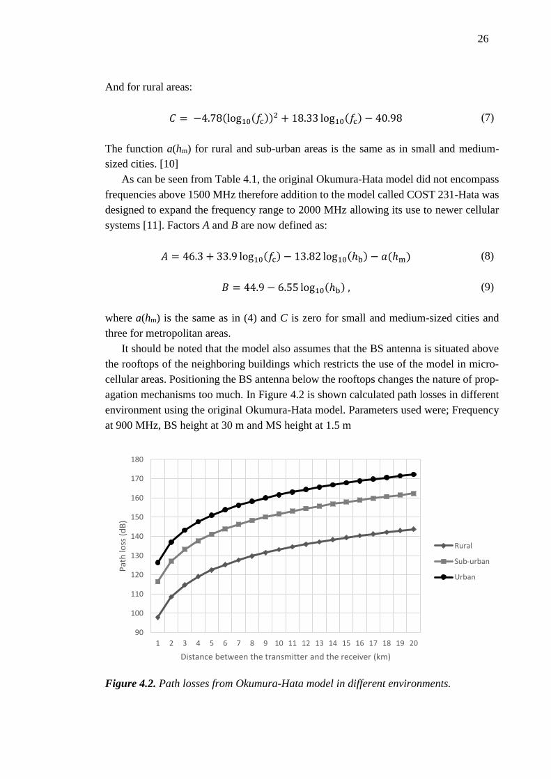
26

And for rural areas:

𝐶 = −4.78(log10(𝑓c))2 + 18.33 log10(𝑓c) − 40.98 (7)

The function a(hm) for rural and sub-urban areas is the same as in small and medium-

sized cities. [10]

As can be seen from Table 4.1, the original Okumura-Hata model did not encompass

frequencies above 1500 MHz therefore addition to the model called COST 231-Hata was

designed to expand the frequency range to 2000 MHz allowing its use to newer cellular

systems [11]. Factors A and B are now defined as:

𝐴 = 46.3 + 33.9 log10(𝑓c) − 13.82 log10(ℎb) − 𝑎(ℎm) (8)

𝐵 = 44.9 − 6.55 log10(ℎb) , (9)

where a(hm) is the same as in (4) and C is zero for small and medium-sized cities and

three for metropolitan areas.

It should be noted that the model also assumes that the BS antenna is situated above

the rooftops of the neighboring buildings which restricts the use of the model in micro-

cellular areas. Positioning the BS antenna below the rooftops changes the nature of prop-

agation mechanisms too much. In Figure 4.2 is shown calculated path losses in different

environment using the original Okumura-Hata model. Parameters used were; Frequency

at 900 MHz, BS height at 30 m and MS height at 1.5 m

Figure 4.2. Path losses from Okumura-Hata model in different environments.

90

100

110

120

130

140

150

160

170

180

1 2 3 4 5 6 7 8 9 10 11 12 13 14 15 16 17 18 19 20

Pat

h lo

ss (

dB

)

Distance between the transmitter and the receiver (km)

Rural

Sub-urban

Urban

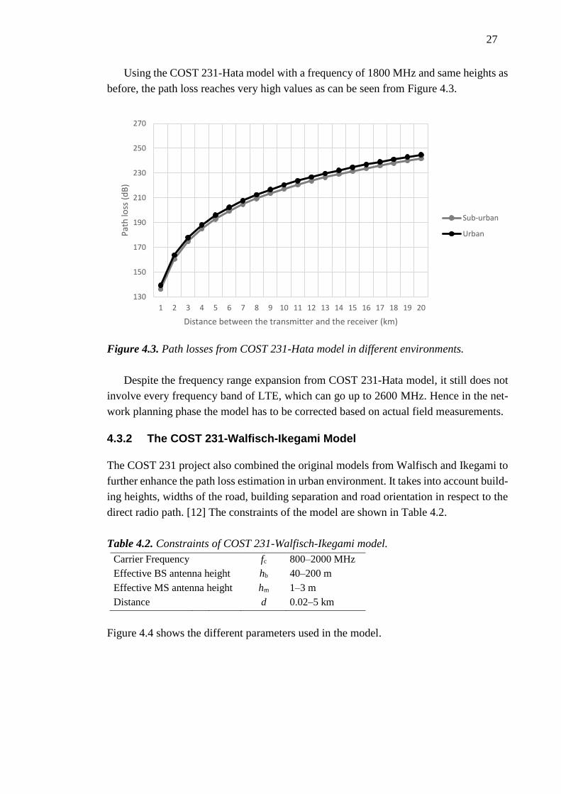
27

Using the COST 231-Hata model with a frequency of 1800 MHz and same heights as

before, the path loss reaches very high values as can be seen from Figure 4.3.

Figure 4.3. Path losses from COST 231-Hata model in different environments.

Despite the frequency range expansion from COST 231-Hata model, it still does not

involve every frequency band of LTE, which can go up to 2600 MHz. Hence in the net-

work planning phase the model has to be corrected based on actual field measurements.

4.3.2 The COST 231-Walfisch-Ikegami Model

The COST 231 project also combined the original models from Walfisch and Ikegami to

further enhance the path loss estimation in urban environment. It takes into account build-

ing heights, widths of the road, building separation and road orientation in respect to the

direct radio path. [12] The constraints of the model are shown in Table 4.2.

Table 4.2. Constraints of COST 231-Walfisch-Ikegami model.

Carrier Frequency fc 800–2000 MHz

Effective BS antenna height hb 40–200 m

Effective MS antenna height hm 1–3 m

Distance d 0.02–5 km

Figure 4.4 shows the different parameters used in the model.

130

150

170

190

210

230

250

270

1 2 3 4 5 6 7 8 9 10 11 12 13 14 15 16 17 18 19 20

Pat

h lo

ss (

dB

)

Distance between the transmitter and the receiver (km)

Sub-urban

Urban

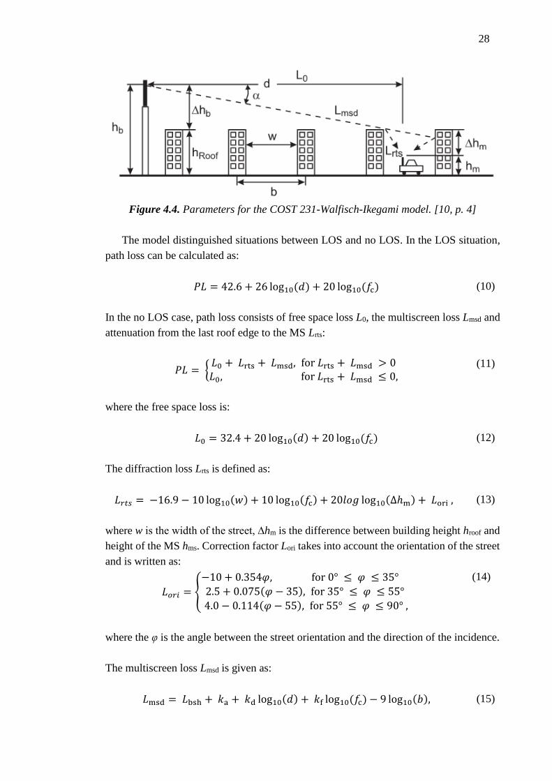
28

Figure 4.4. Parameters for the COST 231-Walfisch-Ikegami model. [10, p. 4]

The model distinguished situations between LOS and no LOS. In the LOS situation,

path loss can be calculated as:

𝑃𝐿 = 42.6 + 26 log10(𝑑) + 20 log10(𝑓c) (10)

In the no LOS case, path loss consists of free space loss L0, the multiscreen loss Lmsd and

attenuation from the last roof edge to the MS Lrts:

𝑃𝐿 = {𝐿0 + 𝐿rts + 𝐿msd, for 𝐿rts + 𝐿msd > 0𝐿0, for 𝐿rts + 𝐿msd ≤ 0,

(11)

where the free space loss is:

𝐿0 = 32.4 + 20 log10(𝑑) + 20 log10(𝑓c) (12)

The diffraction loss Lrts is defined as:

𝐿𝑟𝑡𝑠 = −16.9 − 10 log10(𝑤) + 10 log10(𝑓c) + 20𝑙𝑜𝑔 log10(∆ℎm) + 𝐿ori , (13)

where w is the width of the street, ∆hm is the difference between building height hroof and

height of the MS hms. Correction factor Lori takes into account the orientation of the street

and is written as:

𝐿𝑜𝑟𝑖 = {

−10 + 0.354𝜑, for 0° ≤ 𝜑 ≤ 35°

2.5 + 0.075(𝜑 − 35), for 35° ≤ 𝜑 ≤ 55°

4.0 − 0.114(𝜑 − 55), for 55° ≤ 𝜑 ≤ 90° ,

(14)

where the φ is the angle between the street orientation and the direction of the incidence.

The multiscreen loss Lmsd is given as:

𝐿msd = 𝐿bsh + 𝑘a + 𝑘d log10(𝑑) + 𝑘f log10(𝑓c) − 9 log10(𝑏), (15)

29

where b is the distance between two buildings. The rest of the parameters are as follows:

𝐿bsh = {−18 log10(1 + ∆ℎb), for ℎb > ℎroof

0, for ℎb ≤ ℎroof

(16)

𝑘a = {

54, for ℎb > ℎroof 54 − 0.8∆ℎb, for 𝑑 ≥ 0.5 and ℎb ≤ ℎroof

54 − 0.8∆ℎb𝑑

0.5, for 𝑑 < 0.5 and ℎb ≤ ℎroof ,

(17)

where ∆hb is the difference between heights of the BS and the first building. The path loss

depends on the frequency and distance used, which is taken into account using parameters

kd and kf

𝑘𝑑 = {18, for ℎb > ℎroof

18 − 15 ∆ℎb

ℎroof, for ℎb ≤ ℎroof

(18)

𝑘𝑓 = {0.7 (

𝑓c

925− 1) , for medium − sized cities and sub − urban areas

1.5 (𝑓c

925− 1) , for metropolitan areas

(19)

Figure 4.5 presents simulated path losses using different frequencies and parameters

for the model. The used parameters for different environments are shown in Table 4.3.

Table 4.3. Used parameters for the simulation.

Environment Sub-Urban Metropolitan

BS height (m) 40 50

MS height (m) 2 2

Distance between buildings (m) 50 25

Average building height (m) 15 30

Street width (m) 25 15

Street orientation angle (degrees) 40 30

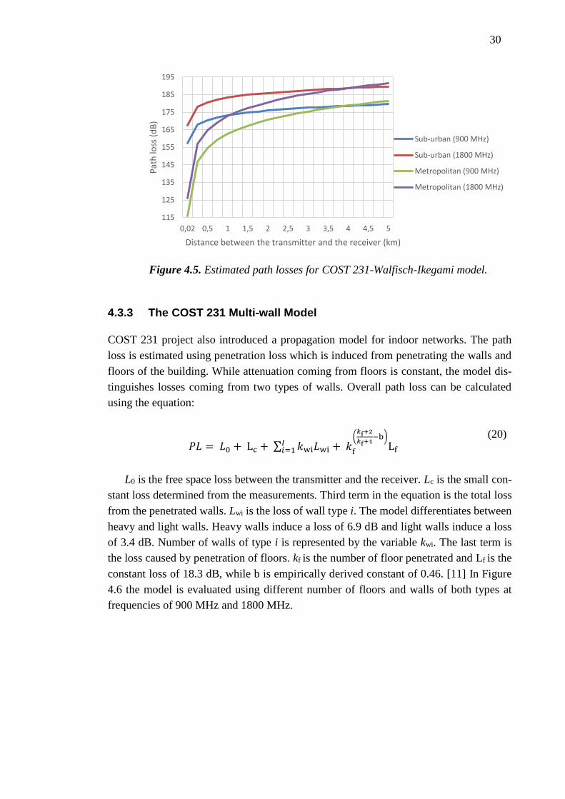
30

Figure 4.5. Estimated path losses for COST 231-Walfisch-Ikegami model.

4.3.3 The COST 231 Multi-wall Model

COST 231 project also introduced a propagation model for indoor networks. The path

loss is estimated using penetration loss which is induced from penetrating the walls and

floors of the building. While attenuation coming from floors is constant, the model dis-

tinguishes losses coming from two types of walls. Overall path loss can be calculated

using the equation:

𝑃𝐿 = 𝐿0 + Lc + ∑ 𝑘wi𝐿wi + 𝑘f

(𝑘f+2

𝑘f+1−b)

Lf𝐼𝑖=1

(20)

L0 is the free space loss between the transmitter and the receiver. Lc is the small con-

stant loss determined from the measurements. Third term in the equation is the total loss

from the penetrated walls. Lwi is the loss of wall type i. The model differentiates between

heavy and light walls. Heavy walls induce a loss of 6.9 dB and light walls induce a loss

of 3.4 dB. Number of walls of type i is represented by the variable kwi. The last term is

the loss caused by penetration of floors. kf is the number of floor penetrated and Lf is the

constant loss of 18.3 dB, while b is empirically derived constant of 0.46. [11] In Figure

4.6 the model is evaluated using different number of floors and walls of both types at

frequencies of 900 MHz and 1800 MHz.

115

125

135

145

155

165

175

185

195

0,02 0,5 1 1,5 2 2,5 3 3,5 4 4,5 5

Pat

h lo

ss (

dB

)

Distance between the transmitter and the receiver (km)

Sub-urban (900 MHz)

Sub-urban (1800 MHz)

Metropolitan (900 MHz)

Metropolitan (1800 MHz)

31

Figure 4.6. Estimated path losses for COST 231 Multi-wall model.

4.3.4 The ITU Model for Indoor Attenuation

The ITU site-general model has similar approach to path loss in indoors as COST 231

Multi-wall model. However this model does not count the loss from the walls separately,

instead the power loss coefficient is changed according to the environment. The model

has a wide frequency range from 900 MHz to 5.2 GHz, but is limited to three floors only

[13]. The total path loss can be estimated using the equation:

𝑃𝐿 = 20 log10(𝑓) + 𝑁 log10(𝑑) + 𝐿f(𝑛) − 28 (21)

Where f is the frequency in megahertz, N is the power loss coefficient, d is the distance

between the transmitter and the receiver in meters, Lf is the floor penetration loss and n is

the number of floors penetrated. The power loss coefficients for common LTE frequen-

cies are represented in Table 4.4 and the floor penetration losses for the same frequencies

are presented in Table 4.5.

Table 4.4. Power loss coefficients for the ITU site-general model.

Frequency Residential Office Commercial

900 MHz - 33 20

1.8–2 GHz 28 30 22

45

55

65

75

85

95

105

115

125

135

1 5 9 13 17 21 25 29 33 37 41 45 49

Pat

h lo

ss (

dB

)

Distance between the transmitter and the receiver (m)

Floors (900 MHz)

Heavy walls (900 MHz)

Light walls (900 MHz)

Floors (1800 MHz)

Heavy walls (1800 MHz)

Light walls (1800 MHz)

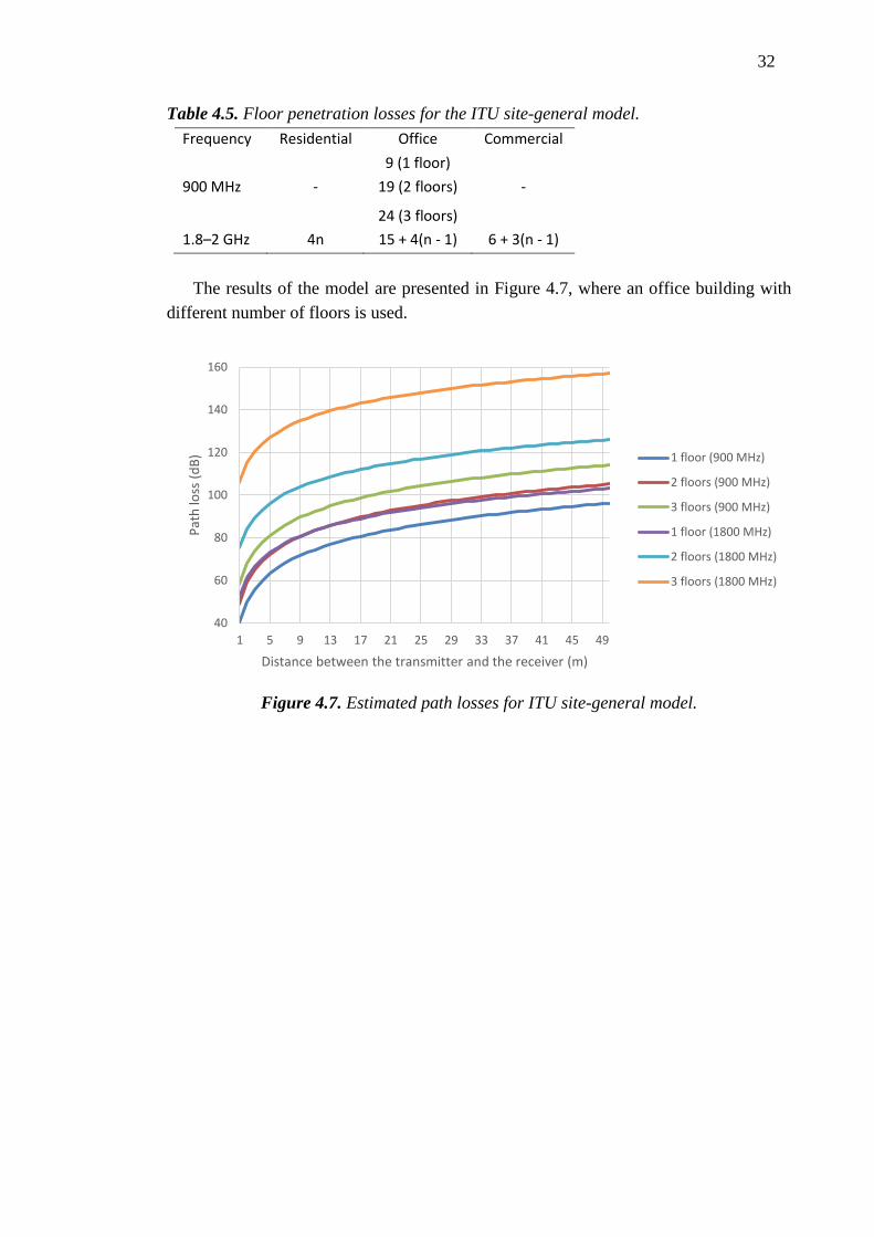
32

Table 4.5. Floor penetration losses for the ITU site-general model.

Frequency Residential Office Commercial

9 (1 floor)

900 MHz - 19 (2 floors) -

24 (3 floors)

1.8–2 GHz 4n 15 + 4(n - 1) 6 + 3(n - 1)

The results of the model are presented in Figure 4.7, where an office building with

different number of floors is used.

Figure 4.7. Estimated path losses for ITU site-general model.

40

60

80

100

120

140

160

1 5 9 13 17 21 25 29 33 37 41 45 49

Pat

h lo

ss (

dB

)

Distance between the transmitter and the receiver (m)

1 floor (900 MHz)

2 floors (900 MHz)

3 floors (900 MHz)

1 floor (1800 MHz)

2 floors (1800 MHz)

3 floors (1800 MHz)

33

5 MEASUREMENTS

The purpose of these measurements is to demonstrate how much the location of the user

affects the overall experience of the user in means of received signal strength and SNR.

Correspondingly, the location of the user also affects the load caused to the network. This

chapter goes through the equipment used in the measurements as well as the different

measurement cases.

5.1 Measurement Equipment and Environment

This measurement campaign is conducted in indoor environment. This is done, because

most of the calls and Internet usage is done in indoors. Measurements are taken in the

Tietotalo of Tampere University of Technology (TUT), which is covered by three macro

cell antennas located in Hermia, approximately 500 meters away, which means that the

measurements are taken in the cell edge area. The network, in which the measurements

are taken, is Nokia’s test network, which operates at 2600 MHz. The network is also used

for test purposes by another party, which may cause unwanted interference to the meas-

urements. The configuration of the base station is represented in Table 5.1.

Table 5.1. eNodeB configuration.

Carrier frequency Band 7 (2600 MHz)

System bandwidth 10 MHz

Transmission power 40 W (46 dBm)

LTE duplex mode FDD

The UE used in the measurements is a Huawei E398 LTE USB modem, which has

the Qualcomm MDM9200TM chipset. The USB modem can be labelled as category three

UE according to 3GPP specifications [14] and it can operate at the LTE frequency bands

of 1800 MHz, 2100 MHz and 2600 MHz with the maximum throughputs of 100 Mbps

and 50 Mbps in the downlink and uplink directions. The modem has the capability of 2 x

2 MIMO operation and supports the LTE modulation schemes of 64-QAM, 16-QAM and

QPSK. [15]

The UE is connected to an IBM Lenovo T 161 laptop with the Windows 7 operating

system. The software used to collect data from the network is Nemo Outdoor version 6.3

and the collected data can be further analysed using the Nemo Analyze version 6.3 soft-

ware. Nemo Outdoor collects all the data exchange between the UE and the base station,

such as radio link performance parameters and data throughput and it is able to present

the recorded data in graphs and tables. More detailed analysis of the data is done using

Excel 2013 and Matlab.

34

The antenna used is Kathrein model 80010543 and the specifications are represented

in Table 5.2.

Table 5.2. Macro cell antenna specification [16].

Frequency range 2300–2690 MHz

Polarization ± 45°

Gain 17.5 dBi

Horizontal Pattern

Half-power beam width 60°–62°

Front-to-back ratio (180° ± 30°) ≥ 25 dB

Cross polar ratio

Main direction 0° Typically: 20 dB

Sector ±60° ≥ 10 dB

Vertical Pattern

Half-power beam width 6.3°–6.5°

Side lobe suppression vertical sector ± 45° > 20 dB

Impedance 50 Ω

VSWR < 1.5

Isolation between ports > 30 dB

Intermodulation IM3 < -150 dBc (2 x 43 dBm carrier)

Max. Power per input 250 W (at 50 °C ambient temperature)

5.2 Measurement Cases

The main parameters measured in these cases were RSRP and SNR. As LTE uses the

adaptive modulation scheme and the current SNR affects the modulation scheme used,

the SNR has a direct effect of the throughput, which is the primary quality indicator for

the user. The RSRP values can be used along with the link budget to calculate benefit for

the operator from the user’s better location.

To get sufficient measurement results, the measurements were taken along various

positions within the Tietotalo building at TUT. This was done so that we can see how

channel conditions vary as the location of the user varies. Static positions were chosen

among places where differences in the received signal quality can be perceived. In these

locations, the measurement equipment was left in place for a period of 5 minutes. The

samples were used to calculate the minimum, median, mean and maximum values of one

location along with the standard deviation (σ) and the cumulative distribution. All the

static locations were repeated on three floors of Tietotalo so that the effects of user loca-

tion between floors can be obtained.

All the measurement points had three different measurement cases. Points 1, 3 and 5

were measured by leaving the measurement equipment at the end of the corridor in the

middle, second case was to see how much signal levels vary if a person was walking

around the measurement equipment in the first location and the final case was to move

35

the equipment away from the end of the corridor approximately 1 meter. Points 2, 4 and

6 were measured next to the wall at both sides of the corridor and the last case was to

move the equipment approximately 1 meter towards the C corridor to a more open space.

The second floor had one point, which other floors did not have and it was used as a

reference point due to its different nature as a wide and clear open space. There the equip-

ment was placed at the left side of the corridor, in the middle of it and finally at the right

side of the corridor.

The previous cases took into account situations within corridors, but to see how much

the location of the user within a room changed the received signal levels, measurements

of static positions were taken there as well. These measurements were done by leaving

the measurement equipment for a period of five minutes near the window, near the door

and between them to see how much variation there were inside of a room.

Measurements were taken in daytime between 10 a.m. and 4 p.m. so variations on

signal levels from movement of other people might be possible.

Every measurement was repeated twice so that more measurement data was generated

for the results to be more accurate. Figure 5.1, Figure 5.2 and Figure 5.3 show the loca-

tions and the numbers where measurements were taken.

Figure 5.1. Measurement points in the second floor of Tietotalo.

Figure 5.2. Measurement points in the third floor of Tietotalo.

36

Figure 5.3. Measurement points in the fourth floor of Tietotalo.

The antennas in Hermia are located in a way that the main beam is coming from the

lower right corner in respect to the figures above. This should lead to stronger signal

levels especially in points 1, 2 and 4 in the upper floors.

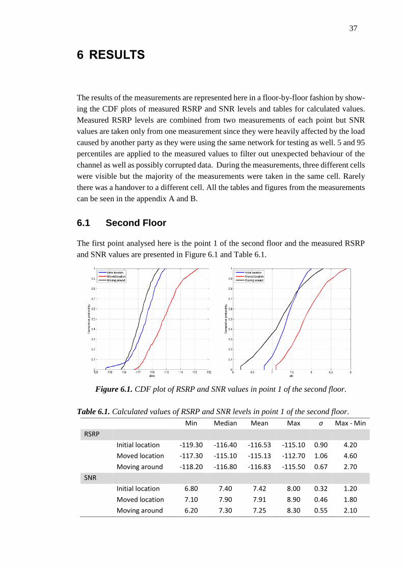
37

6 RESULTS

The results of the measurements are represented here in a floor-by-floor fashion by show-

ing the CDF plots of measured RSRP and SNR levels and tables for calculated values.

Measured RSRP levels are combined from two measurements of each point but SNR

values are taken only from one measurement since they were heavily affected by the load

caused by another party as they were using the same network for testing as well. 5 and 95

percentiles are applied to the measured values to filter out unexpected behaviour of the

channel as well as possibly corrupted data. During the measurements, three different cells

were visible but the majority of the measurements were taken in the same cell. Rarely

there was a handover to a different cell. All the tables and figures from the measurements

can be seen in the appendix A and B.

6.1 Second Floor

The first point analysed here is the point 1 of the second floor and the measured RSRP

and SNR values are presented in Figure 6.1 and Table 6.1.

Figure 6.1. CDF plot of RSRP and SNR values in point 1 of the second floor.

Table 6.1. Calculated values of RSRP and SNR levels in point 1 of the second floor.

Min Median Mean Max σ Max - Min

RSRP

Initial location -119.30 -116.40 -116.53 -115.10 0.90 4.20

Moved location -117.30 -115.10 -115.13 -112.70 1.06 4.60

Moving around -118.20 -116.80 -116.83 -115.50 0.67 2.70

SNR

Initial location 6.80 7.40 7.42 8.00 0.32 1.20

Moved location 7.10 7.90 7.91 8.90 0.46 1.80

Moving around 6.20 7.30 7.25 8.30 0.55 2.10

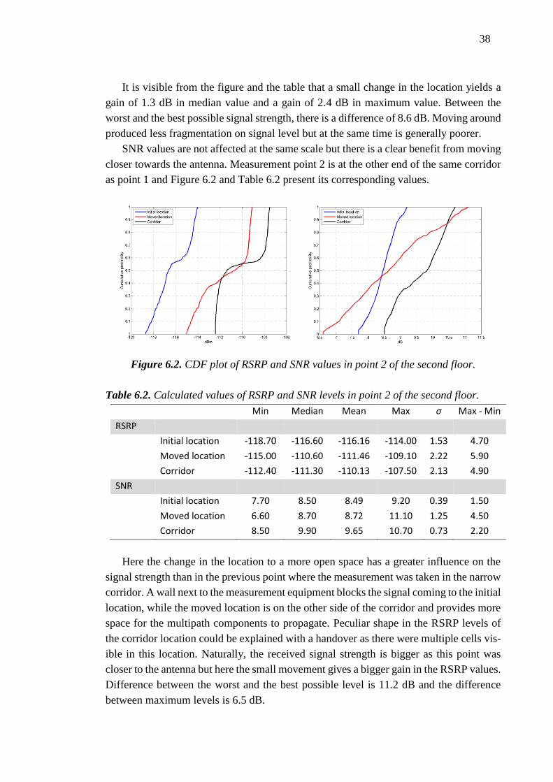
38

It is visible from the figure and the table that a small change in the location yields a

gain of 1.3 dB in median value and a gain of 2.4 dB in maximum value. Between the

worst and the best possible signal strength, there is a difference of 8.6 dB. Moving around

produced less fragmentation on signal level but at the same time is generally poorer.

SNR values are not affected at the same scale but there is a clear benefit from moving

closer towards the antenna. Measurement point 2 is at the other end of the same corridor

as point 1 and Figure 6.2 and Table 6.2 present its corresponding values.

Figure 6.2. CDF plot of RSRP and SNR values in point 2 of the second floor.

Table 6.2. Calculated values of RSRP and SNR levels in point 2 of the second floor.

Min Median Mean Max σ Max - Min

RSRP

Initial location -118.70 -116.60 -116.16 -114.00 1.53 4.70

Moved location -115.00 -110.60 -111.46 -109.10 2.22 5.90

Corridor -112.40 -111.30 -110.13 -107.50 2.13 4.90

SNR

Initial location 7.70 8.50 8.49 9.20 0.39 1.50

Moved location 6.60 8.70 8.72 11.10 1.25 4.50

Corridor 8.50 9.90 9.65 10.70 0.73 2.20

Here the change in the location to a more open space has a greater influence on the

signal strength than in the previous point where the measurement was taken in the narrow

corridor. A wall next to the measurement equipment blocks the signal coming to the initial

location, while the moved location is on the other side of the corridor and provides more

space for the multipath components to propagate. Peculiar shape in the RSRP levels of

the corridor location could be explained with a handover as there were multiple cells vis-

ible in this location. Naturally, the received signal strength is bigger as this point was

closer to the antenna but here the small movement gives a bigger gain in the RSRP values.

Difference between the worst and the best possible level is 11.2 dB and the difference

between maximum levels is 6.5 dB.

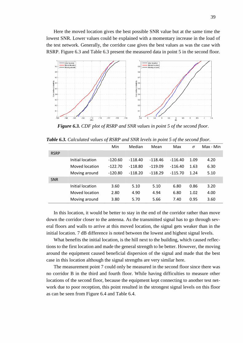
39

Here the moved location gives the best possible SNR value but at the same time the

lowest SNR. Lower values could be explained with a momentary increase in the load of

the test network. Generally, the corridor case gives the best values as was the case with

RSRP. Figure 6.3 and Table 6.3 present the measured data in point 5 in the second floor.

Figure 6.5. CDF plot of RSRP values in point 5 of the second floor.

Table 6.5. Calculated values of RSRP levels in point 5 of the second floor.

Figure 6.3. CDF plot of RSRP and SNR values in point 5 of the second floor.

Table 6.3. Calculated values of RSRP and SNR levels in point 5 of the second floor.

Min Median Mean Max σ Max - Min

RSRP

Initial location -120.60 -118.40 -118.46 -116.40 1.09 4.20

Moved location -122.70 -118.80 -119.09 -116.40 1.63 6.30

Moving around -120.80 -118.20 -118.29 -115.70 1.24 5.10

SNR

Initial location 3.60 5.10 5.10 6.80 0.86 3.20

Moved location 2.80 4.90 4.94 6.80 1.02 4.00

Moving around 3.80 5.70 5.66 7.40 0.95 3.60

In this location, it would be better to stay in the end of the corridor rather than move

down the corridor closer to the antenna. As the transmitted signal has to go through sev-

eral floors and walls to arrive at this moved location, the signal gets weaker than in the

initial location. 7 dB difference is noted between the lowest and highest signal levels.

What benefits the initial location, is the hill next to the building, which caused reflec-

tions to the first location and made the general strength to be better. However, the moving

around the equipment caused beneficial dispersion of the signal and made that the best

case in this location although the signal strengths are very similar here.

The measurement point 7 could only be measured in the second floor since there was

no corridor B in the third and fourth floor. While having difficulties to measure other

locations of the second floor, because the equipment kept connecting to another test net-

work due to poor reception, this point resulted in the strongest signal levels on this floor

as can be seen from Figure 6.4 and Table 6.4.

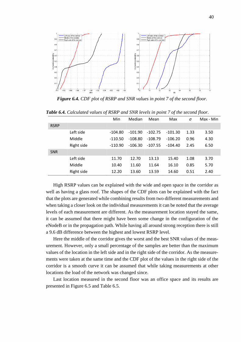
40

Figure 6.7. CDF plot of RSRP values in point 7 of the second floor.

Figure 6.4. CDF plot of RSRP and SNR values in point 7 of the second floor.

Table 6.4. Calculated values of RSRP and SNR levels in point 7 of the second floor.

Min Median Mean Max σ Max - Min

RSRP

Left side -104.80 -101.90 -102.75 -101.30 1.33 3.50

Middle -110.50 -108.80 -108.79 -106.20 0.96 4.30

Right side -110.90 -106.30 -107.55 -104.40 2.45 6.50

SNR

Left side 11.70 12.70 13.13 15.40 1.08 3.70

Middle 10.40 11.60 11.64 16.10 0.85 5.70

Right side 12.20 13.60 13.59 14.60 0.51 2.40

High RSRP values can be explained with the wide and open space in the corridor as

well as having a glass roof. The shapes of the CDF plots can be explained with the fact

that the plots are generated while combining results from two different measurements and

when taking a closer look on the individual measurements it can be noted that the average

levels of each measurement are different. As the measurement location stayed the same,

it can be assumed that there might have been some change in the configuration of the

eNodeB or in the propagation path. While having all around strong reception there is still

a 9.6 dB difference between the highest and lowest RSRP level.

Here the middle of the corridor gives the worst and the best SNR values of the meas-

urement. However, only a small percentage of the samples are better than the maximum

values of the location in the left side and in the right side of the corridor. As the measure-

ments were taken at the same time and the CDF plot of the values in the right side of the

corridor is a smooth curve it can be assumed that while taking measurements at other

locations the load of the network was changed since.

Last location measured in the second floor was an office space and its results are

presented in Figure 6.5 and Table 6.5.

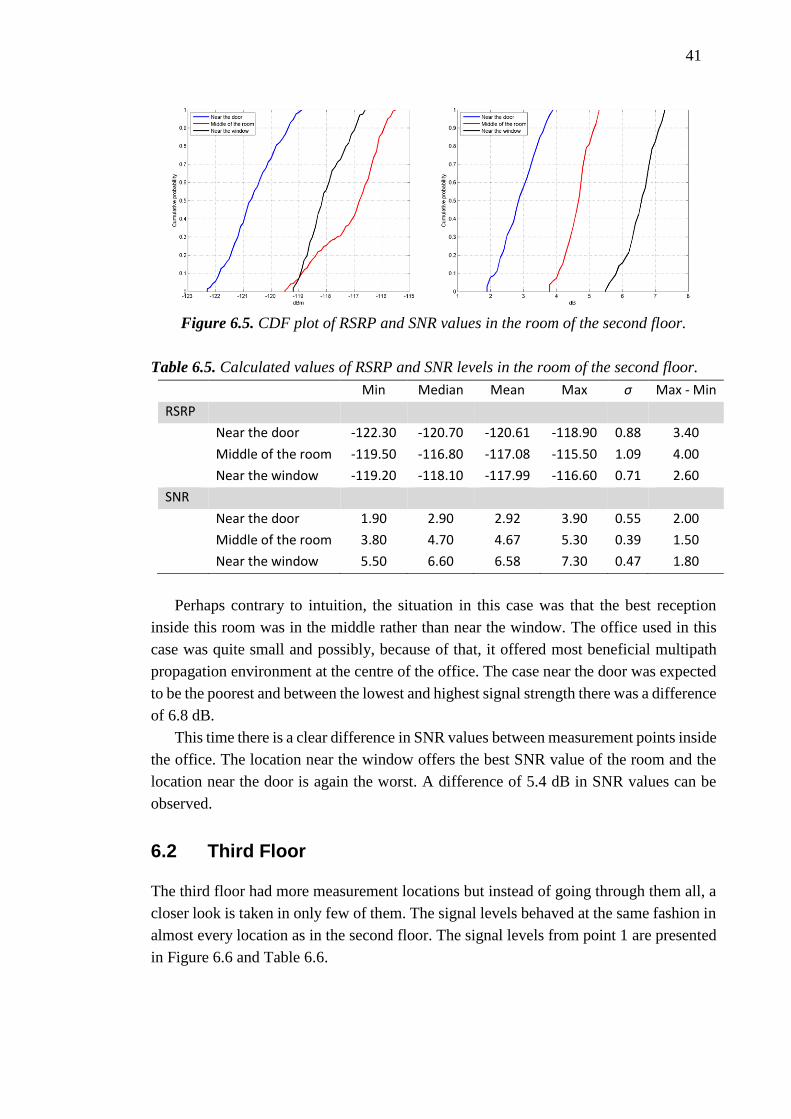
41

Figure 6.9. CDF plot of RSRP values in the room of the second floor.

Figure 6.5. CDF plot of RSRP and SNR values in the room of the second floor.

Table 6.5. Calculated values of RSRP and SNR levels in the room of the second floor.

Min Median Mean Max σ Max - Min

RSRP

Near the door -122.30 -120.70 -120.61 -118.90 0.88 3.40

Middle of the room -119.50 -116.80 -117.08 -115.50 1.09 4.00

Near the window -119.20 -118.10 -117.99 -116.60 0.71 2.60

SNR

Near the door 1.90 2.90 2.92 3.90 0.55 2.00

Middle of the room 3.80 4.70 4.67 5.30 0.39 1.50

Near the window 5.50 6.60 6.58 7.30 0.47 1.80

Perhaps contrary to intuition, the situation in this case was that the best reception

inside this room was in the middle rather than near the window. The office used in this

case was quite small and possibly, because of that, it offered most beneficial multipath

propagation environment at the centre of the office. The case near the door was expected

to be the poorest and between the lowest and highest signal strength there was a difference

of 6.8 dB.

This time there is a clear difference in SNR values between measurement points inside

the office. The location near the window offers the best SNR value of the room and the

location near the door is again the worst. A difference of 5.4 dB in SNR values can be

observed.

6.2 Third Floor

The third floor had more measurement locations but instead of going through them all, a

closer look is taken in only few of them. The signal levels behaved at the same fashion in

almost every location as in the second floor. The signal levels from point 1 are presented

in Figure 6.6 and Table 6.6.

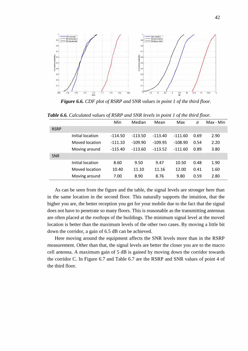
42

Figure 6.11. CDF plot of RSRP values in point 1 of the third floor.

Figure 6.6. CDF plot of RSRP and SNR values in point 1 of the third floor.

Table 6.6. Calculated values of RSRP and SNR levels in point 1 of the third floor.

Min Median Mean Max σ Max - Min

RSRP

Initial location -114.50 -113.50 -113.40 -111.60 0.69 2.90

Moved location -111.10 -109.90 -109.95 -108.90 0.54 2.20

Moving around -115.40 -113.60 -113.52 -111.60 0.89 3.80

SNR

Initial location 8.60 9.50 9.47 10.50 0.48 1.90

Moved location 10.40 11.10 11.16 12.00 0.41 1.60

Moving around 7.00 8.90 8.76 9.80 0.59 2.80

As can be seen from the figure and the table, the signal levels are stronger here than

in the same location in the second floor. This naturally supports the intuition, that the

higher you are, the better reception you get for your mobile due to the fact that the signal

does not have to penetrate so many floors. This is reasonable as the transmitting antennas

are often placed at the rooftops of the buildings. The minimum signal level at the moved

location is better than the maximum levels of the other two cases. By moving a little bit

down the corridor, a gain of 6.5 dB can be achieved.

Here moving around the equipment affects the SNR levels more than in the RSRP

measurement. Other than that, the signal levels are better the closer you are to the macro

cell antenna. A maximum gain of 5 dB is gained by moving down the corridor towards

the corridor C. In Figure 6.7 and Table 6.7 are the RSRP and SNR values of point 4 of

the third floor.

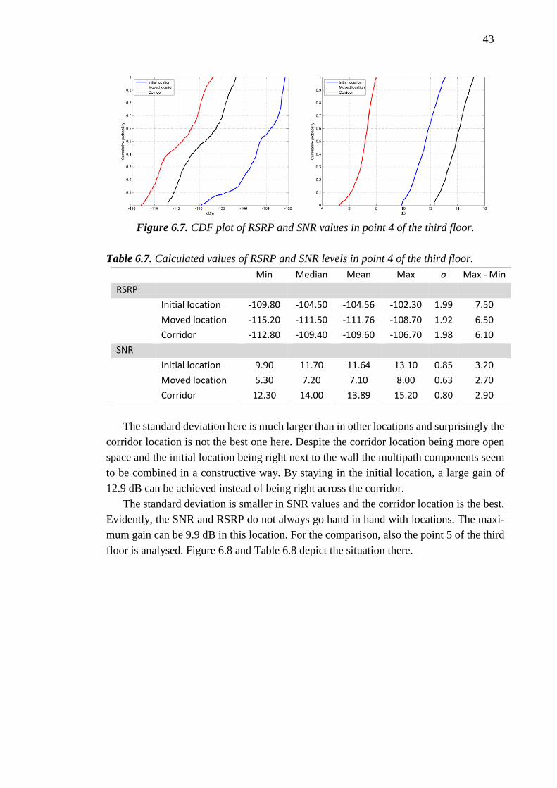
43

Figure 6.7. CDF plot of RSRP and SNR values in point 4 of the third floor.

Table 6.7. Calculated values of RSRP and SNR levels in point 4 of the third floor.

Min Median Mean Max σ Max - Min

RSRP

Initial location -109.80 -104.50 -104.56 -102.30 1.99 7.50

Moved location -115.20 -111.50 -111.76 -108.70 1.92 6.50

Corridor -112.80 -109.40 -109.60 -106.70 1.98 6.10

SNR

Initial location 9.90 11.70 11.64 13.10 0.85 3.20

Moved location 5.30 7.20 7.10 8.00 0.63 2.70

Corridor 12.30 14.00 13.89 15.20 0.80 2.90

The standard deviation here is much larger than in other locations and surprisingly the

corridor location is not the best one here. Despite the corridor location being more open

space and the initial location being right next to the wall the multipath components seem

to be combined in a constructive way. By staying in the initial location, a large gain of

12.9 dB can be achieved instead of being right across the corridor.

The standard deviation is smaller in SNR values and the corridor location is the best.

Evidently, the SNR and RSRP do not always go hand in hand with locations. The maxi-

mum gain can be 9.9 dB in this location. For the comparison, also the point 5 of the third

floor is analysed. Figure 6.8 and Table 6.8 depict the situation there.

44

Figure 6.8. CDF plot of RSRP and SNR values in point 5 of the third floor.

Table 6.8. Calculated values of RSRP and SNR levels in point 5 of the third floor.

Min Median Mean Max σ Max - Min

RSRP

Initial location -120.80 -119.20 -119.16 -117.50 0.81 3.30

Moved location -121.00 -118.70 -118.79 -116.90 0.97 4.10

Moving around -121.30 -119.40 -119.39 -117.50 0.98 3.80

SNR

Initial location 2.90 4.50 4.55 6.00 0.75 3.10

Moved location 2.70 4.60 4.62 6.50 0.83 3.80

Moving around 2.50 4.10 4.17 6.00 0.86 3.50

Despite being higher in the building, the RSRP levels are close to the ones in the

second floor. However, the signal is not so fragmented, as the standard deviation is

smaller here. Moving down the corridor towards the corridor C is beneficial here unlike

in the second floor. The maximum benefit in RSRP level here is 4.4 dB.

Again, there is little variation on signal levels and the moved location results the

strongest signal strengths here. Difference between the minimum and maximum is 4 dB

on SNR levels. Last location analysed on the third floor is the office room and its RSRP

levels are presented in Figure 6.9 and Table 6.9.

Figure 6.9. CDF plot of RSRP and SNR values in the room of the third floor.

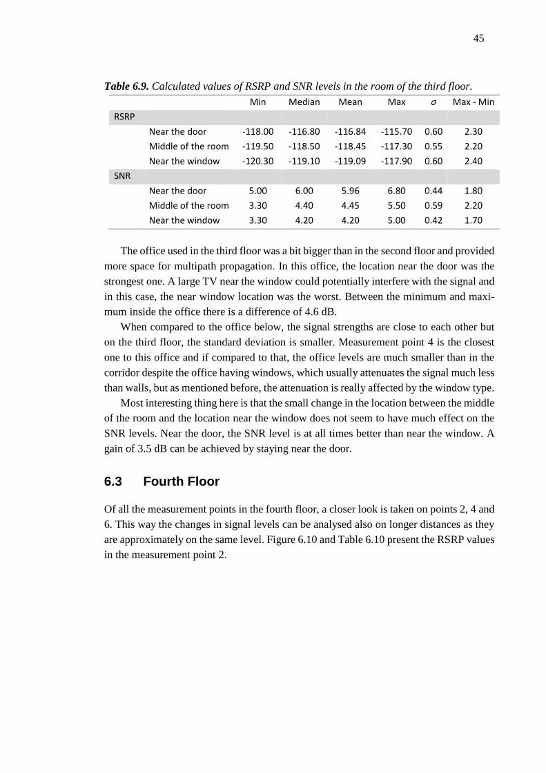
45

Table 6.9. Calculated values of RSRP and SNR levels in the room of the third floor.

Min Median Mean Max σ Max - Min

RSRP

Near the door -118.00 -116.80 -116.84 -115.70 0.60 2.30

Middle of the room -119.50 -118.50 -118.45 -117.30 0.55 2.20

Near the window -120.30 -119.10 -119.09 -117.90 0.60 2.40

SNR

Near the door 5.00 6.00 5.96 6.80 0.44 1.80

Middle of the room 3.30 4.40 4.45 5.50 0.59 2.20

Near the window 3.30 4.20 4.20 5.00 0.42 1.70

The office used in the third floor was a bit bigger than in the second floor and provided

more space for multipath propagation. In this office, the location near the door was the

strongest one. A large TV near the window could potentially interfere with the signal and

in this case, the near window location was the worst. Between the minimum and maxi-

mum inside the office there is a difference of 4.6 dB.

When compared to the office below, the signal strengths are close to each other but

on the third floor, the standard deviation is smaller. Measurement point 4 is the closest

one to this office and if compared to that, the office levels are much smaller than in the

corridor despite the office having windows, which usually attenuates the signal much less

than walls, but as mentioned before, the attenuation is really affected by the window type.

Most interesting thing here is that the small change in the location between the middle

of the room and the location near the window does not seem to have much effect on the

SNR levels. Near the door, the SNR level is at all times better than near the window. A

gain of 3.5 dB can be achieved by staying near the door.

6.3 Fourth Floor

Of all the measurement points in the fourth floor, a closer look is taken on points 2, 4 and

6. This way the changes in signal levels can be analysed also on longer distances as they

are approximately on the same level. Figure 6.10 and Table 6.10 present the RSRP values

in the measurement point 2.

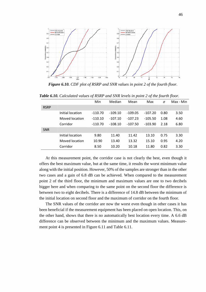
46

Figure 6.10. CDF plot of RSRP and SNR values in point 2 of the fourth floor.

Table 6.10. Calculated values of RSRP and SNR levels in point 2 of the fourth floor.

Min Median Mean Max σ Max - Min

RSRP

Initial location -110.70 -109.10 -109.05 -107.20 0.80 3.50

Moved location -110.10 -107.10 -107.23 -105.50 1.08 4.60

Corridor -110.70 -108.10 -107.50 -103.90 2.18 6.80

SNR

Initial location 9.80 11.40 11.42 13.10 0.75 3.30

Moved location 10.90 13.40 13.32 15.10 0.95 4.20

Corridor 8.50 10.20 10.18 11.80 0.82 3.30

At this measurement point, the corridor case is not clearly the best, even though it

offers the best maximum value, but at the same time, it results the worst minimum value

along with the initial position. However, 50% of the samples are stronger than in the other

two cases and a gain of 6.8 dB can be achieved. When compared to the measurement

point 2 of the third floor, the minimum and maximum values are one to two decibels

bigger here and when comparing to the same point on the second floor the difference is

between two to eight decibels. There is a difference of 14.8 dB between the minimum of

the initial location on second floor and the maximum of corridor on the fourth floor.

The SNR values of the corridor are now the worst even though in other cases it has

been beneficial if the measurement equipment has been placed on open location. This, on

the other hand, shows that there is no automatically best location every time. A 6.6 dB

difference can be observed between the minimum and the maximum values. Measure-

ment point 4 is presented in Figure 6.11 and Table 6.11.

47

Figure 6.11. CDF plot of RSRP and SNR values in point 4 of the fourth floor.

Table 6.11. Calculated values of RSRP and SNR levels in point 4 of the fourth floor.

Min Median Mean Max σ Max - Min

RSRP

Initial location -113.20 -111.20 -110.98 -109.00 1.24 4.20

Moved location -115.70 -112.80 -112.85 -109.90 0.93 5.80

Corridor -114.00 -111.00 -111.20 -109.10 1.21 4.90

SNR

Initial location 4.10 6.60 6.57 8.10 0.96 4.00

Moved location 4.70 6.60 6.62 9.00 0.83 4.30

Corridor 7.60 10.30 9.93 11.30 1.06 3.70

At this point, the initial location and the location on the corridor results in similar

signal strengths, while the moved location is the worst. Minimum values have dropped

2.5 dB to 5 dB and the maximum values 1.8 dB to 5.1 dB when compared to point 2 of

the same floor. Quite surprisingly, the RSRP values on the third floor at the same point

are stronger both in the minimum and maximum sense. A 6.7 dB difference can be ob-

served within this location and only 1.7 dB gain from the worst location in point 2. When

comparing the maximum value for point 2 and the minimum of this point, the benefit is

11.8 dB in favour of point 2.

While the initial location and the moved location give similar results, the corridor

location in now clearly the best. This now supports the assumption that the received SNR

levels are better in open locations but from the previous cases it was noted that the as-

sumption is not always correct. A gain of 7.2 dB in SNR can be observed. The last corri-

dor measurement point analysed here is point 6 and its RSRP values are depicted in Figure

6.12 and Table 6.12.

48

Figure 6.12. CDF plot of RSRP and SNR values in point 6 of the fourth floor.

Table 6.12. Calculated values of RSRP and SNR levels in point 6 of the fourth floor.

Min Median Mean Max σ Max - Min

RSRP

Initial location -116.30 -113.50 -113.66 -112.10 0.96 4.20

Moved location -121.30 -118.60 -118.72 -116.50 1.20 4.80

Corridor -117.00 -114.30 -114.26 -106.80 1.54 10.20

SNR

Initial location 7.10 8.20 8.19 9.30 0.52 2.20

Moved location 0.60 4.70 4.40 5.90 1.28 5.30

Corridor 8.00 9.00 8.96 9.70 0.38 1.70

The corridor now gives the maximum RSRP value of this point but there are only 5%

of the samples, which are bigger than the maximum of the initial location maximum thus

generally, the initial location is better. Naturally, the minimum and the maximum levels

are lower here than in the points 2 and 4 of this floor as the distance grows from the

transmitter. However, this time the respective values are bigger than in the same point of

the third floor. A maximum gain of 15.1 dB can be achieved on the fourth floor if com-

pared to the third floor and a gain of 14.6 dB within this point. The maximum RSRP value

of the second point of this floor is 17.6 dB bigger than the minimum of this point.

Even though the samples were filtered through 5 and 95 percentiles, the moved loca-

tion gave unnaturally low SNR values. This might be due to temporary increase in the

load of the test network due to another party’s ongoing tests. However, it does not change

the fact that the moved location is now the worst but rather give too large gain between

the maximum and minimum values, which now is 9.1 dB. The final location analysed in

the results is the office used on the fourth floor. RSRP and SNR values of that location

are in Figure 6.13 and Table 6.13.

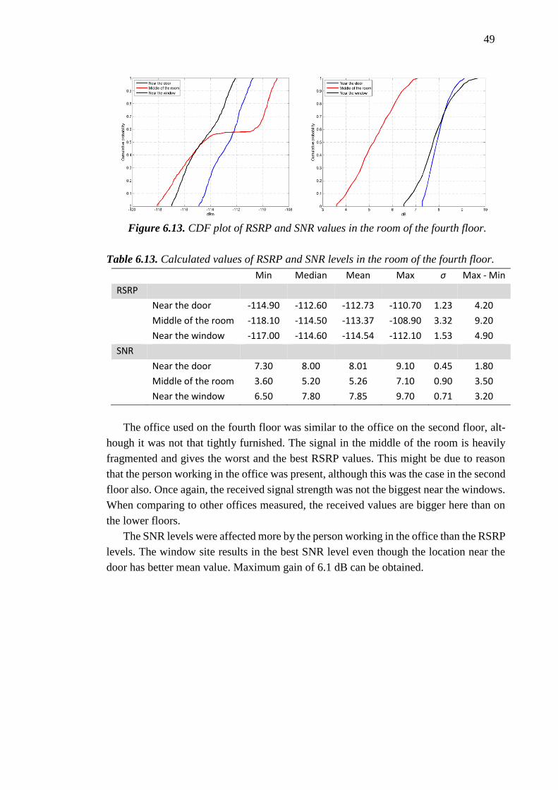
49

Figure 6.13. CDF plot of RSRP and SNR values in the room of the fourth floor.

Table 6.13. Calculated values of RSRP and SNR levels in the room of the fourth floor.

Min Median Mean Max σ Max - Min

RSRP

Near the door -114.90 -112.60 -112.73 -110.70 1.23 4.20

Middle of the room -118.10 -114.50 -113.37 -108.90 3.32 9.20

Near the window -117.00 -114.60 -114.54 -112.10 1.53 4.90

SNR

Near the door 7.30 8.00 8.01 9.10 0.45 1.80

Middle of the room 3.60 5.20 5.26 7.10 0.90 3.50

Near the window 6.50 7.80 7.85 9.70 0.71 3.20

The office used on the fourth floor was similar to the office on the second floor, alt-

hough it was not that tightly furnished. The signal in the middle of the room is heavily

fragmented and gives the worst and the best RSRP values. This might be due to reason

that the person working in the office was present, although this was the case in the second

floor also. Once again, the received signal strength was not the biggest near the windows.

When comparing to other offices measured, the received values are bigger here than on

the lower floors.

The SNR levels were affected more by the person working in the office than the RSRP

levels. The window site results in the best SNR level even though the location near the

door has better mean value. Maximum gain of 6.1 dB can be obtained.

50

7 CONCLUSIONS

This thesis focused on the effects of the user location in LTE networks and as the meas-

ured signals were coming from outdoor, this corresponds to the common situation when

using the mobile phone. After the measurements were conducted, several observations

could be made.

As it turns out, a small change in location can make a big difference. RSRP and SNR

values get stronger when moving to a more open space. This seems to benefit the addition

of multipath components in the receiver. Naturally, respective values get stronger when

moving towards the transmitting antenna. This however, can be hard for the user to know,

as the locations of the base stations are often unknown to the user. There are some appli-

cations, at least for Android devices, that enables the user to see the received signal

strengths and the approximate location of the base station.

When measuring signal levels inside offices, probably the most surprising result was

that the RSRP levels were not the strongest near the windows as that is the common con-

ception. However, SNR levels were generally better near the windows.

RSRP and SNR levels grow stronger when the user moves to upper floors. This is

natural as the transmitting antennas are often located at rooftops of buildings. This leads

to poor reception in the lower floors and in the basements. The UE transmit power is

partly affected by the path loss [17], therefore it is beneficial to stay in areas where the

received signal strength is strong.

Fragmentation of the received signal is greater when moving around the equipment

and often resulted in lower minimum levels in SNR and RSRP measurements. This would

suggest that the user should prefer locations where there are no people around. In rare

cases, moving around the equipment resulted in better signal strengths. Inside the meas-

ured offices, the location on the middle of the room was the most fragmented.

The gains in SNR levels are more significant than the gains of same scale in RSRP.

The Channel Quality Indicator (CQI) reported by the UE affects the modulation scheme

used. The higher the CQI, the better modulation scheme is used and therefore higher data

rates are achieved. How the UE determines the CQI is UE specific and there is no univer-

sal way to map the SINR to CQI. However, there has been a study, which mapped SNR

values to CQI in different antenna settings [18].

Using those results as a baseline, it can be seen that there is approximately 2 dB dif-

ference between CQI ranks and in many cases of the measurements, the gain between

different locations was more than 5 dBs and up to 10 dBs. CQI ranks from the measure-

ments vary from 0 to 10. When those CQI ranks are mapped to modulation schemes used

according to the specifications [17] it can be seen that the modulation schemes used in

the measurements vary from no transmission, as the SNR is too low, to 64-QAM. Using

the 64-QAM modulation does not automatically mean that the bit rate is the highest pos-

sible as there are different coding rates from different modulation schemes as well.

51

When mapping these modulation schemes to data rates an increase from CQI rank 1

to CQI rank 3 would increase the maximum throughput from 1.1 Mbps to 2.51 Mbps on

a 10 MHz bandwidth as was the case in these measurements. Increase in CQI increases

the throughput approximately 2 Mbps, although it is not linear and at higher ranks, the

increase in throughput is between three and four Mbps at each increment in CQI. The

average gain in SNR values between every measurement location was 5.7 dB, which

means an increase of approximately two ranks.

The network planning is a complicated process and it is a constant balancing between

capacity, coverage, and building costs. Especially, when planning indoor coverage with-

out additional indoor antenna elements, the additional building losses quickly increase

the number of cell sites required in the planned area.

As mentioned, the signal is the strongest near the outer walls of the building and on

the higher floors. The problem is that currently there is no way for the operator to encour-

age subscribers to move to areas of better reception. One possibility could be that the

operator could change the pricing of phone calls depending on the signal quality levels

where the phone call is made, and at the same time provide the subscribers easy to use

application for the smart phone to check the signal levels at the current location.

Just by reducing the building loss to save money in the deployment phase of the net-

work will just lead to areas of no reception and unhappy customers. In the news article

by Talouselämä [19], illegally installed and misconfigured repeaters may cause serious

problems in the network, nevertheless they can be bought from retail shops. One solution

might be that the operator would provide extra antennas indoors or Home eNodeBs to

ensure coverage indoors while planning the network without additional building losses.

After all, it is hard to make subscribers move to a different area to make a phone call as

people want to use their phone when they want and where they want.

When planning the coverage of the network, an estimate of a cell range can be calcu-

lated from the path loss. Using the path loss value from the Table 3.1. adding a building

loss of 20 dB, and using Cost 231-Hata model to calculate the cell range, the resulting

range is 1.1 km. The total coverage of a 3-sector site is 2.5 km2. From all the locations

measured resulted on the average gain of 7.5 dB between the worst and the best value in

RSRP. If reducing the building loss by that gain, the resulting coverage of a site becomes

6.3 km2. Hence, the coverage is 2.5 bigger than the original, which means that when plan-

ning for a 100 km2 area the original plan uses 40 sites to cover the whole area, while the

plan with reduced losses uses only 16 sites. If a site costs 20000€, there is a save of 480000

€.

As the measurements were not taken in laboratory conditions, errors are possible in

the measured values. Sometimes there were people walking by the measurement equip-

ment which could have an effect on the signal strengths but as they passed by quickly

there should not be large distortions on the values and after all the values were filtered

using the 5% and 95% percentiles. Perhaps the largest errors would have become from

the changes on the configuration of eNodeB and the transmitting antennas but I were not

aware of such changes therefore it is really just a possibility.

52

When thinking of user’s location indoors, the best place to be is an open space and as

high as possible where there are no people around. As these measurements were taken in

in one building only, further measurements should be taken to verify these results. It is

expected that similar results are highly probable.

53

REFERENCES

[1] Holma Harri, Toskala Antti. LTE for UMTS: Evolution to LTE-Advanced. Sec-

ond Edition. United Kingdom 2011, John Wiley & Sons, Ltd. 543 p.

[2] 3GPP. Requirements for Evolved UTRA (E-UTRA) and Evolved UTRAN (E-

UTRAN). 2005, TR 25.913, version 7.0.0. 15 p.

[3] 3GPP. Network Architecture. 2011, TS 23.002, version 8.7.0 Release 8. 90 p.

[4] 3GPP. Universal Mobile Telecommunications System (UMTS); Technical Spec-

ifications and Technical Reports for a UTRAN-based 3GPP system. 2009, TS

21.101, version 8.0.0 Release 8. 42 p.

[5] Penttinen Jyrki. The LTE/SAE Deployment Handbook. United Kingdom 2012,

John Wiley & Sons, Ltd. 411 p.

[6] Syed Abdul Basit. Dimensioning of LTE Network. Description of Models and

Tools, Coverage and Capacity Estimation of 3GPP Long Term Evolution. Hel-

sinki 2009. Helsinki University of Technology, Department of Electrical and

Communications Engineering. 71 p.

[7] Niemelä Jarno, Asp Ari, Sydorov Yaroslav. Radiosignaalin vaimennusmittauksia

nykyaikaisissa asuintaloissa. Tampere 2012. Tampere University of Technology,

Department of Communications Engineering. 62 p.

[8] Ari Asp, Yaroslav Sydorov, Mikko Keskikastari, Mikko Valkama, Jarno Niemelä.

Impact of Modern Construction Materials on Radio Signal Propagation: Practical

Measurements and Network Planning Aspects. Tampere 2014. Tampere Univer-

sity of Technology, Department of Electronics and Communications Engineering.

7 p.

[9] Singal T. L. Wireless Communications. Delhi 2010, Tata McGraw Hill Education

Private Ltd. 673 p.

[10] Hata Masaharu. Empirical Formula for Propagation Loss in Land Mobile Radio

Services. IEEE Transactions on Vehicular Technology 29(1980)3, pp. 317 – 325.

[11] COST 231. Digital mobile radio towards future generation systems. 1999, Euro-

pean Commission. 474 p.

[12] The COST 231–Walfish–Ikegami model. Appendix 7.B. In: Molisch, Andreas F.

Wireless Communications. Second Edition. United Kingdom, 2011. 10 p.

[13] ITU, Recommendation ITU-R P.1238-7, Propagation data and prediction methods

for the planning of indoor radio communication systems and radio local area net-

works in the frequency range 900 MHz to 100 GHz. Geneva 2012. 26 p.

[14] 3GPP. User Equipment (UE) radio access capabilities. 2011, TS 36.206 version

10.2.0 Release 10. 22 p.

[15] Huawei. Huawei E398 specifications [WWW]. [accessed on 1.4.2014]. Available

at: http://support.huawei.com/ecommunity/bbs/10182143.html

[16] Kathrein-Werke KG. 80010543 specifications [WWW]. [accessed on 26.6.2014].

Available at: http://www.antennasystems.com/Merchant2/pdf/800_10543.pdf

54

[17] 3GPP. Evolved Universal Terrestrial Radio Access (E-UTRA); Physical layer

procedures. 2014, TS 36.213 version 11.7.0 Release 11. 183 p.

[18] Mohammad T. Kawser, Nafiz Imtiaz Bin Hamid, Nayeemul Hasan, M. Shah

Alam, M. Musfiqur Rahman. Downlink SNR to CQI Mapping for Different Mul-

tiple Antenna Techniques in LTE. International Journal of Information and

Electronics Engineering 2(2012)5, pp. 757-760.

[19] Talouselämä. Eikö matkapuhelimesi kuulu sisällä? Kaupat myyvät helpotusta,

mutta jos käytät sitä, poliisi kolkuttaa oveasi [WWW]. [accessed on 25.7.2014].

Available in Finnish at: http://www.talouselama.fi/uutiset/eiko+matkapu-

helimesi+kuulu+sisalla+kaupat+myyvat+helpotusta+mutta+jos+kaytat+sita+po-

liisi+kolkuttaa+oveasi/a2256229#commentsList

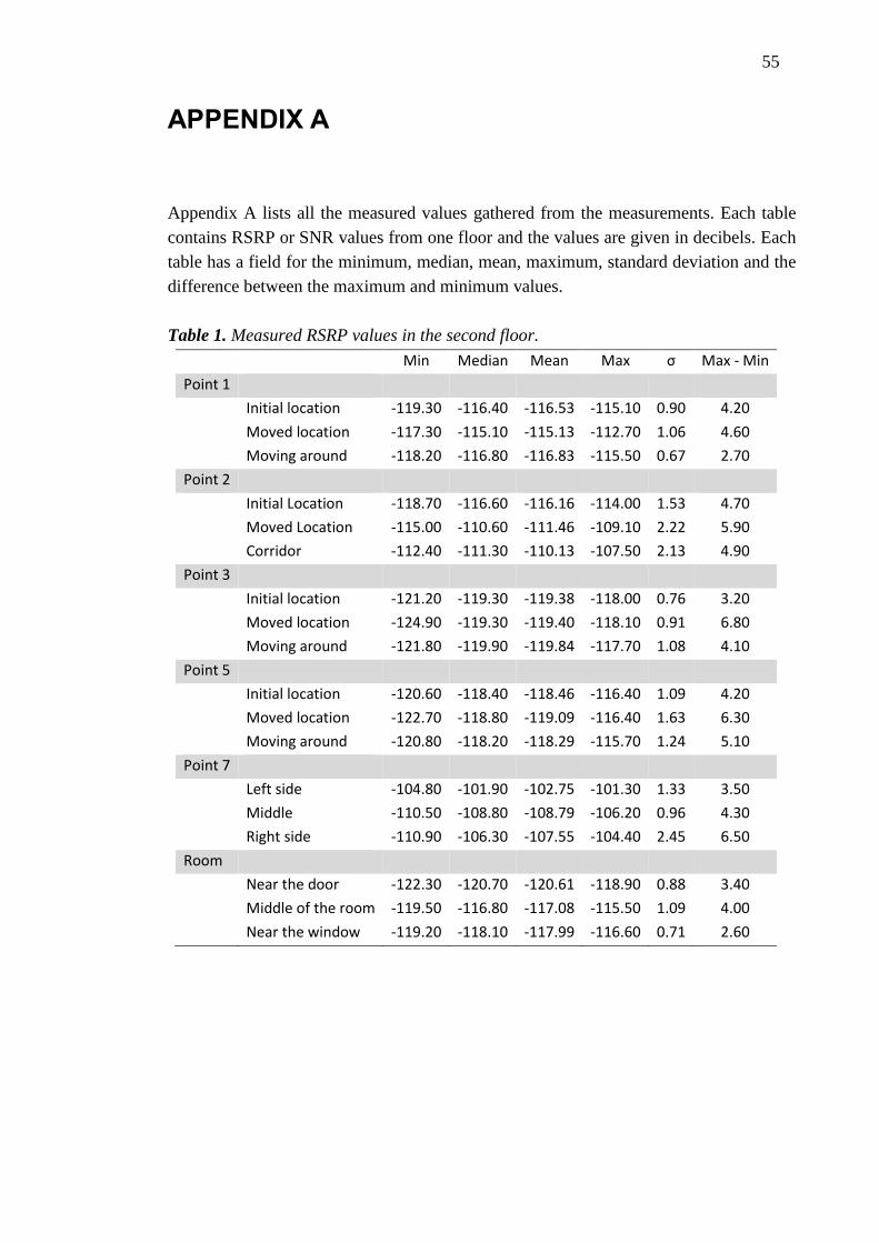
55

APPENDIX A

Appendix A lists all the measured values gathered from the measurements. Each table

contains RSRP or SNR values from one floor and the values are given in decibels. Each

table has a field for the minimum, median, mean, maximum, standard deviation and the

difference between the maximum and minimum values.

Table 1. Measured RSRP values in the second floor.

Min Median Mean Max σ Max - Min

Point 1

Initial location -119.30 -116.40 -116.53 -115.10 0.90 4.20

Moved location -117.30 -115.10 -115.13 -112.70 1.06 4.60

Moving around -118.20 -116.80 -116.83 -115.50 0.67 2.70

Point 2

Initial Location -118.70 -116.60 -116.16 -114.00 1.53 4.70

Moved Location -115.00 -110.60 -111.46 -109.10 2.22 5.90

Corridor -112.40 -111.30 -110.13 -107.50 2.13 4.90

Point 3

Initial location -121.20 -119.30 -119.38 -118.00 0.76 3.20

Moved location -124.90 -119.30 -119.40 -118.10 0.91 6.80

Moving around -121.80 -119.90 -119.84 -117.70 1.08 4.10

Point 5

Initial location -120.60 -118.40 -118.46 -116.40 1.09 4.20

Moved location -122.70 -118.80 -119.09 -116.40 1.63 6.30

Moving around -120.80 -118.20 -118.29 -115.70 1.24 5.10

Point 7

Left side -104.80 -101.90 -102.75 -101.30 1.33 3.50

Middle -110.50 -108.80 -108.79 -106.20 0.96 4.30

Right side -110.90 -106.30 -107.55 -104.40 2.45 6.50

Room

Near the door -122.30 -120.70 -120.61 -118.90 0.88 3.40

Middle of the room -119.50 -116.80 -117.08 -115.50 1.09 4.00

Near the window -119.20 -118.10 -117.99 -116.60 0.71 2.60

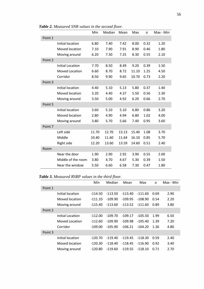
56

Table 2. Measured SNR values in the second floor.

Min Median Mean Max σ Max - Min

Point 1

Initial location 6.80 7.40 7.42 8.00 0.32 1.20

Moved location 7.10 7.90 7.91 8.90 0.46 1.80

Moving around 6.20 7.30 7.25 8.30 0.55 2.10

Point 2

Initial Location 7.70 8.50 8.49 9.20 0.39 1.50

Moved Location 6.60 8.70 8.72 11.10 1.25 4.50

Corridor 8.50 9.90 9.65 10.70 0.73 2.20

Point 3

Initial location 4.40 5.10 5.13 5.80 0.37 1.40

Moved location 3.20 4.40 4.37 5.50 0.56 2.30

Moving around 3.50 5.00 4.92 6.20 0.66 2.70

Point 5

Initial location 3.60 5.10 5.10 6.80 0.86 3.20

Moved location 2.80 4.90 4.94 6.80 1.02 4.00

Moving around 3.80 5.70 5.66 7.40 0.95 3.60

Point 7

Left side 11.70 12.70 13.13 15.40 1.08 3.70

Middle 10.40 11.60 11.64 16.10 0.85 5.70

Right side 12.20 13.60 13.59 14.60 0.51 2.40

Room

Near the door 1.90 2.90 2.92 3.90 0.55 2.00

Middle of the room 3.80 4.70 4.67 5.30 0.39 1.50

Near the window 5.50 6.60 6.58 7.30 0.47 1.80

Table 3. Measured RSRP values in the third floor.

Min Median Mean Max σ Max - Min

Point 1

Initial location -114.50 -113.50 -113.40 -111.60 0.69 2.90

Moved location -111.10 -109.90 -109.95 -108.90 0.54 2.20

Moving around -115.40 -113.60 -113.52 -111.60 0.89 3.80

Point 2

Initial Location -112.00 -109.70 -109.17 -105.50 1.99 6.50

Moved Location -112.60 -109.90 -109.98 -105.40 1.39 7.20

Corridor -109.00 -105.90 -106.21 -104.20 1.36 4.80

Point 3

Initial location -120.70 -119.40 -119.45 -118.30 0.59 2.40

Moved location -120.30 -118.40 -118.45 -116.90 0.92 3.40

Moving around -120.80 -119.60 -119.55 -118.10 0.71 2.70

57

Min Median Mean Max σ Max - Min

Point 4

Initial Location -109.80 -104.50 -104.56 -102.30 1.99 7.50

Moved Location -115.20 -111.50 -111.76 -108.70 1.92 6.50

Corridor -112.80 -109.40 -109.60 -106.70 1.98 6.10

Point 5

Initial location -120.80 -119.20 -119.16 -117.50 0.81 3.30

Moved location -121.00 -118.70 -118.79 -116.90 0.97 4.10

Moving around -121.30 -119.40 -119.39 -117.50 0.98 3.80

Point 6

Initial Location -120.80 -118.60 -118.75 -117.00 0.93 3.80

Moved Location -121.90 -118.00 -118.37 -115.20 2.00 6.70

Corridor -116.60 -114.80 -114.50 -111.60 1.39 5.00

Room

Near the door -118.00 -116.80 -116.84 -115.70 0.60 2.30

Middle of the room -119.50 -118.50 -118.45 -117.30 0.55 2.20

Near the window -120.30 -119.10 -119.09 -117.90 0.60 2.40

Table 4. Measured SNR values in the third floor.

Min Median Mean Max σ Max - Min

Point 1

Initial location 8.60 9.50 9.47 10.50 0.48 1.90

Moved location 10.40 11.10 11.16 12.00 0.41 1.60

Moving around 7.00 8.90 8.76 9.80 0.59 2.80

Point 2

Initial Location 11.10 13.70 13.64 15.40 1.00 4.30

Moved Location 7.50 8.70 9.10 11.80 1.20 4.30

Corridor 13.30 14.80 14.82 16.50 0.75 3.20

Point 3

Initial location 2.50 4.10 4.05 5.10 0.62 2.60

Moved location 4.90 5.70 5.67 6.50 0.44 1.60

Moving around 3.00 4.00 3.98 5.00 0.48 2.00

Point 4

Initial Location 9.90 11.70 11.64 13.10 0.85 3.20

Moved Location 5.30 7.20 7.10 8.00 0.63 2.70

Corridor 12.30 14.00 13.89 15.20 0.80 2.90

Point 5

Initial location 2.90 4.50 4.55 6.00 0.75 3.10

Moved location 2.70 4.60 4.62 6.50 0.83 3.80

Moving around 2.50 4.10 4.17 6.00 0.86 3.50

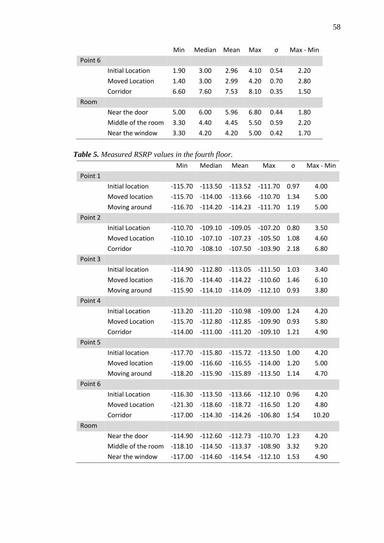
58

Min Median Mean Max σ Max - Min

Point 6

Initial Location 1.90 3.00 2.96 4.10 0.54 2.20

Moved Location 1.40 3.00 2.99 4.20 0.70 2.80

Corridor 6.60 7.60 7.53 8.10 0.35 1.50

Room

Near the door 5.00 6.00 5.96 6.80 0.44 1.80

Middle of the room 3.30 4.40 4.45 5.50 0.59 2.20

Near the window 3.30 4.20 4.20 5.00 0.42 1.70

Table 5. Measured RSRP values in the fourth floor.

Min Median Mean Max σ Max - Min

Point 1

Initial location -115.70 -113.50 -113.52 -111.70 0.97 4.00

Moved location -115.70 -114.00 -113.66 -110.70 1.34 5.00

Moving around -116.70 -114.20 -114.23 -111.70 1.19 5.00

Point 2

Initial Location -110.70 -109.10 -109.05 -107.20 0.80 3.50

Moved Location -110.10 -107.10 -107.23 -105.50 1.08 4.60

Corridor -110.70 -108.10 -107.50 -103.90 2.18 6.80

Point 3

Initial location -114.90 -112.80 -113.05 -111.50 1.03 3.40

Moved location -116.70 -114.40 -114.22 -110.60 1.46 6.10

Moving around -115.90 -114.10 -114.09 -112.10 0.93 3.80

Point 4

Initial Location -113.20 -111.20 -110.98 -109.00 1.24 4.20

Moved Location -115.70 -112.80 -112.85 -109.90 0.93 5.80

Corridor -114.00 -111.00 -111.20 -109.10 1.21 4.90

Point 5

Initial location -117.70 -115.80 -115.72 -113.50 1.00 4.20

Moved location -119.00 -116.60 -116.55 -114.00 1.20 5.00

Moving around -118.20 -115.90 -115.89 -113.50 1.14 4.70

Point 6

Initial Location -116.30 -113.50 -113.66 -112.10 0.96 4.20

Moved Location -121.30 -118.60 -118.72 -116.50 1.20 4.80

Corridor -117.00 -114.30 -114.26 -106.80 1.54 10.20

Room

Near the door -114.90 -112.60 -112.73 -110.70 1.23 4.20

Middle of the room -118.10 -114.50 -113.37 -108.90 3.32 9.20

Near the window -117.00 -114.60 -114.54 -112.10 1.53 4.90

59

Table 6. Measured SNR values in the fourth floor.

Min Median Mean Max σ Max - Min

Point 1

Initial location 7.40 8.60 8.60 10.00 0.66 2.60

Moved location 2.60 9.40 8.80 11.20 1.97 8.60

Moving around 6.90 8.40 8.41 9.90 0.77 3.00

Point 2

Initial Location 9.80 11.40 11.42 13.10 0.75 3.30

Moved Location 10.90 13.40 13.32 15.10 0.95 4.20

Corridor 8.50 10.20 10.18 11.80 0.82 3.30

Point 3

Initial location 8.50 9.30 9.34 10.10 0.40 1.60

Moved location 7.00 10.50 10.10 11.60 1.24 4.60

Moving around 8.30 9.70 9.71 11.00 0.65 2.70

Point 4

Initial Location 4.10 6.60 6.57 8.10 0.96 4.00

Moved Location 4.70 6.60 6.62 9.00 0.83 4.30

Corridor 7.60 10.30 9.93 11.30 1.06 3.70

Point 5

Initial location 6.20 7.80 7.72 9.00 0.70 2.80

Moved location 4.60 6.30 6.27 7.90 0.86 3.30

Moving around 5.80 7.60 7.55 9.00 0.81 3.20

Point 6

Initial Location 7.10 8.20 8.19 9.30 0.52 2.20

Moved Location 0.60 4.70 4.40 5.90 1.28 5.30

Corridor 8.00 9.00 8.96 9.70 0.38 1.70

Room

Near the door 7.30 8.00 8.01 9.10 0.45 1.80

Middle of the room 3.60 5.20 5.26 7.10 0.90 3.50

Near the window 6.50 7.80 7.85 9.70 0.71 3.20

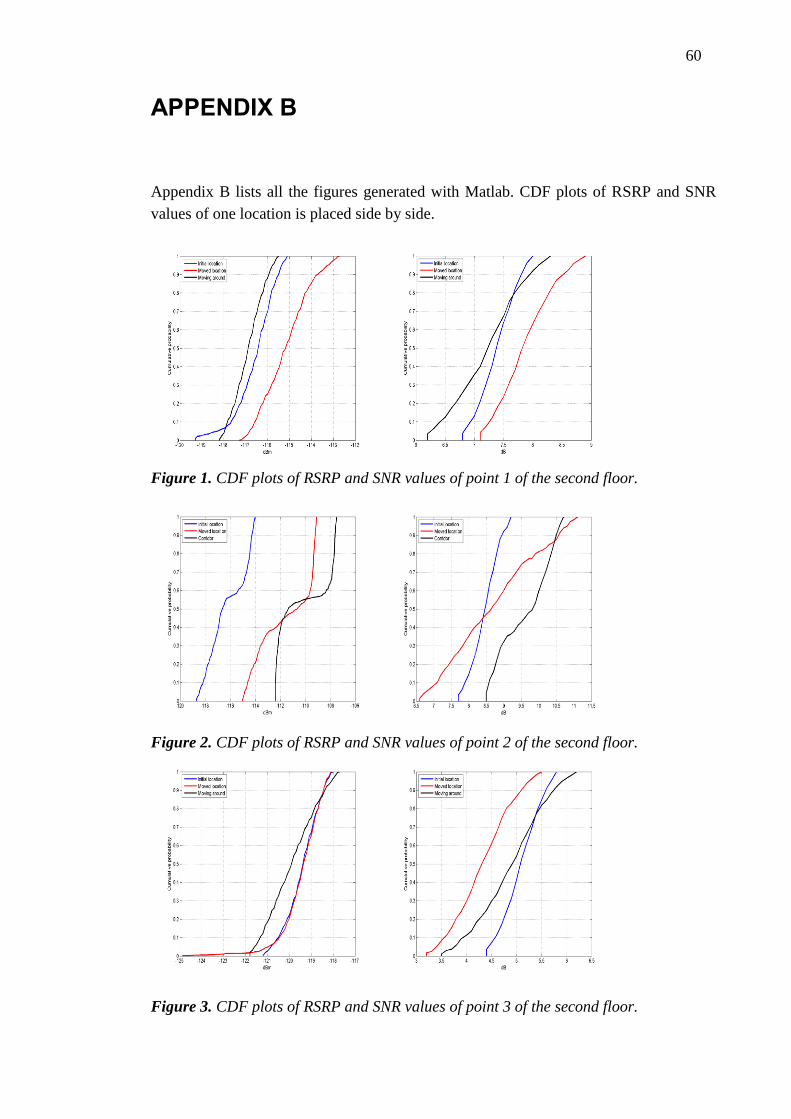
60

APPENDIX B

Appendix B lists all the figures generated with Matlab. CDF plots of RSRP and SNR

values of one location is placed side by side.

Figure 1. CDF plots of RSRP and SNR values of point 1 of the second floor.

Figure 2. CDF plots of RSRP and SNR values of point 2 of the second floor.

Figure 3. CDF plots of RSRP and SNR values of point 3 of the second floor.

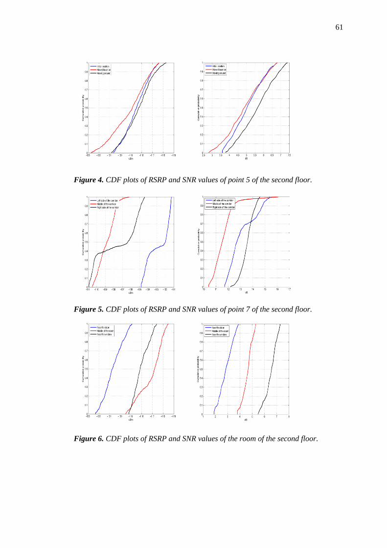
61

Figure 4. CDF plots of RSRP and SNR values of point 5 of the second floor.

Figure 5. CDF plots of RSRP and SNR values of point 7 of the second floor.

Figure 6. CDF plots of RSRP and SNR values of the room of the second floor.

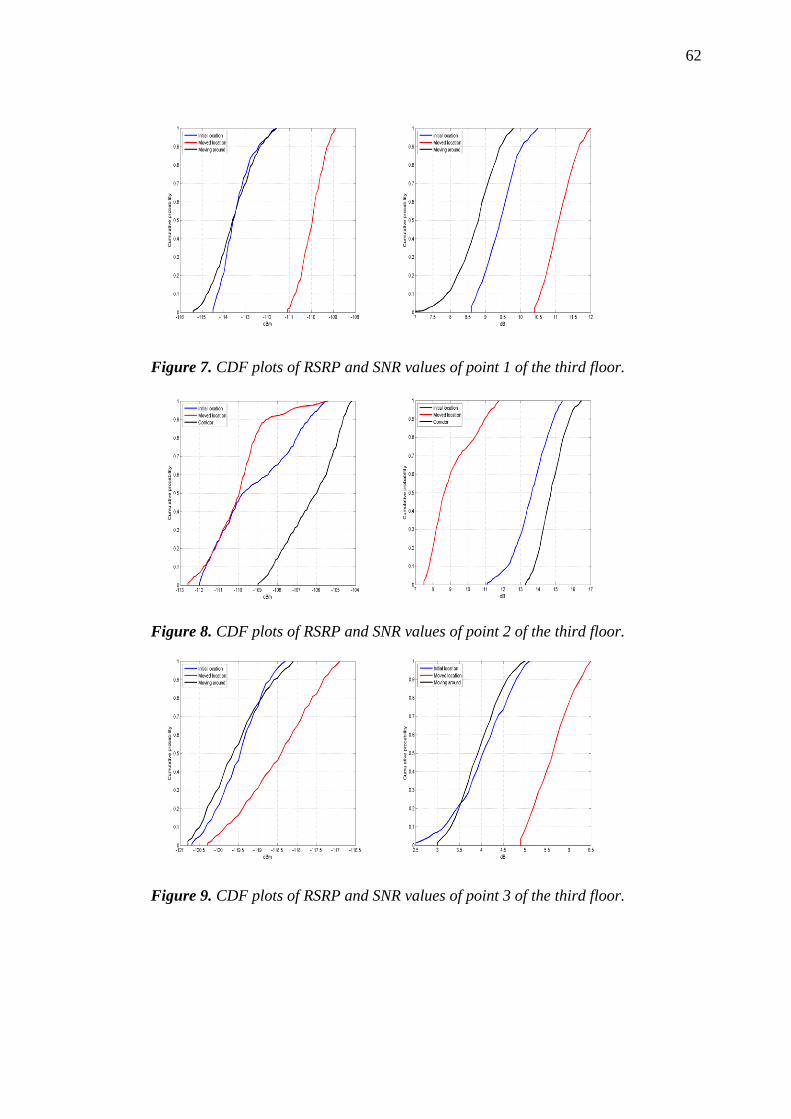
62

Figure 7. CDF plots of RSRP and SNR values of point 1 of the third floor.

Figure 8. CDF plots of RSRP and SNR values of point 2 of the third floor.

Figure 9. CDF plots of RSRP and SNR values of point 3 of the third floor.

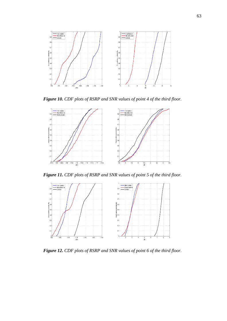
63

Figure 10. CDF plots of RSRP and SNR values of point 4 of the third floor.

Figure 11. CDF plots of RSRP and SNR values of point 5 of the third floor.

Figure 12. CDF plots of RSRP and SNR values of point 6 of the third floor.

64

Figure 13. CDF plots of RSRP and SNR values of the room of the third floor.

Figure 14. CDF plots of RSRP and SNR values of point 1 of the fourth floor.

Figure 15. CDF plots of RSRP and SNR values of point 2 of the fourth floor.

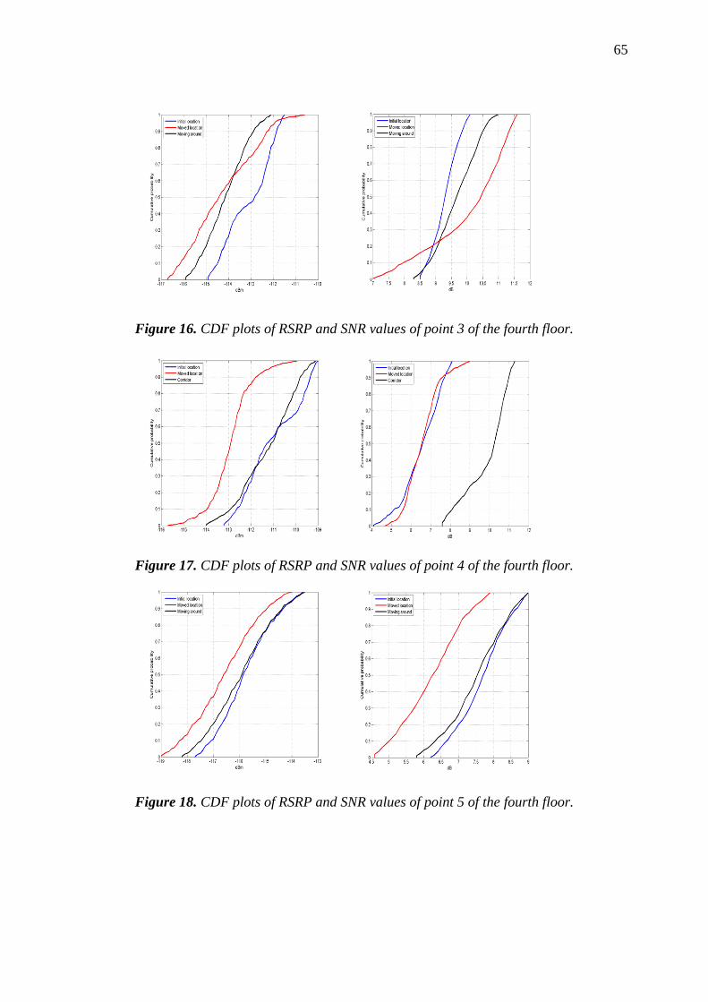
65

Figure 16. CDF plots of RSRP and SNR values of point 3 of the fourth floor.

Figure 17. CDF plots of RSRP and SNR values of point 4 of the fourth floor.

Figure 18. CDF plots of RSRP and SNR values of point 5 of the fourth floor.

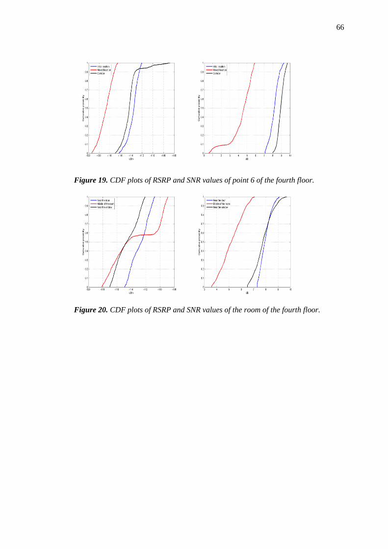
66

Figure 19. CDF plots of RSRP and SNR values of point 6 of the fourth floor.

Figure 20. CDF plots of RSRP and SNR values of the room of the fourth floor.