large zx-calculus for the working quantum computer scientist
TRANSCRIPT

ZX-calculus for the working quantum computer scientistJohn van de Wetering1,2
1Radboud Universiteit Nijmegen2Oxford UniversityDecember 29, 2020
The ZX-calculus is a graphical language for reasoning about quantum com-putation that has recently seen an increased usage in a variety of areas such asquantum circuit optimisation, surface codes and lattice surgery, measurement-based quantum computation, and quantum foundations. The first half of thisreview gives a gentle introduction to the ZX-calculus suitable for those fa-miliar with the basics of quantum computing. The aim here is to make thereader comfortable enough with the ZX-calculus that they could use it in theirdaily work for small computations on quantum circuits and states. The lat-ter sections give a condensed overview of the literature on the ZX-calculus.We discuss Clifford computation and graphically prove the Gottesman-Knilltheorem, we discuss a recently introduced extension of the ZX-calculus thatallows for convenient reasoning about Toffoli gates, and we discuss the recentcompleteness theorems for the ZX-calculus that show that, in principle, allreasoning about quantum computation can be done using ZX-diagrams. Ad-ditionally, we discuss the categorical and algebraic origins of the ZX-calculusand we discuss several extensions of the language which can represent mixedstates, measurement, classical control and higher-dimensional qudits.
Contents1 Introduction 3
1.1 Overview of the paper . . . . . . . . . . . . . . . . . . . . . . . . . . . . . . 41.2 Tools and resources . . . . . . . . . . . . . . . . . . . . . . . . . . . . . . . . 5
2 Quantum circuits vs ZX-diagrams 62.1 From quantum circuits to ZX-diagrams . . . . . . . . . . . . . . . . . . . . 62.2 States in the ZX-calculus . . . . . . . . . . . . . . . . . . . . . . . . . . . . 72.3 Hadamards and colour changing . . . . . . . . . . . . . . . . . . . . . . . . 8
3 ZX-diagrams 93.1 Spiders . . . . . . . . . . . . . . . . . . . . . . . . . . . . . . . . . . . . . . . 93.2 Composition . . . . . . . . . . . . . . . . . . . . . . . . . . . . . . . . . . . 113.3 Symmetries . . . . . . . . . . . . . . . . . . . . . . . . . . . . . . . . . . . . 133.4 Scalars . . . . . . . . . . . . . . . . . . . . . . . . . . . . . . . . . . . . . . . 153.5 Adjoints, transpose and conjugate . . . . . . . . . . . . . . . . . . . . . . . 163.6 Hadamards . . . . . . . . . . . . . . . . . . . . . . . . . . . . . . . . . . . . 17
John van de Wetering: [email protected], http://vdwetering.name
1
arX
iv:2
012.
1396
6v1
[qu
ant-
ph]
27
Dec
202
0

3.7 Universality . . . . . . . . . . . . . . . . . . . . . . . . . . . . . . . . . . . . 18
4 The ZX-calculus 184.1 Spider fusion and identity removal . . . . . . . . . . . . . . . . . . . . . . . 194.2 The copy rule and π-commutation . . . . . . . . . . . . . . . . . . . . . . . 204.3 Formal rewriting and soundness . . . . . . . . . . . . . . . . . . . . . . . . . 224.4 Colour changing . . . . . . . . . . . . . . . . . . . . . . . . . . . . . . . . . 234.5 The bialgebra and Hopf rule . . . . . . . . . . . . . . . . . . . . . . . . . . . 244.6 The complete calculus . . . . . . . . . . . . . . . . . . . . . . . . . . . . . . 27
5 Some example derivations 285.1 GHZ-preparation circuit . . . . . . . . . . . . . . . . . . . . . . . . . . . . . 295.2 Pauli pushing . . . . . . . . . . . . . . . . . . . . . . . . . . . . . . . . . . . 295.3 Magic state injection . . . . . . . . . . . . . . . . . . . . . . . . . . . . . . . 305.4 Teleportation . . . . . . . . . . . . . . . . . . . . . . . . . . . . . . . . . . . 305.5 Detecting entanglement . . . . . . . . . . . . . . . . . . . . . . . . . . . . . 315.6 Phase polynomials and phase gadgets . . . . . . . . . . . . . . . . . . . . . 32
6 Clifford computation 346.1 Graph states . . . . . . . . . . . . . . . . . . . . . . . . . . . . . . . . . . . 356.2 Graph-like diagrams . . . . . . . . . . . . . . . . . . . . . . . . . . . . . . . 366.3 Measurement-based quantum computation . . . . . . . . . . . . . . . . . . . 376.4 Local complementation and pivoting . . . . . . . . . . . . . . . . . . . . . . 396.5 Simplification of Clifford ZX-diagrams . . . . . . . . . . . . . . . . . . . . . 406.6 From ZX-diagrams to circuits . . . . . . . . . . . . . . . . . . . . . . . . . . 41
7 ZX-diagrams, categorically 437.1 Category theory background . . . . . . . . . . . . . . . . . . . . . . . . . . . 437.2 Interpretation of a ZX-diagram . . . . . . . . . . . . . . . . . . . . . . . . . 447.3 Rewriting and completeness . . . . . . . . . . . . . . . . . . . . . . . . . . . 457.4 !-boxes . . . . . . . . . . . . . . . . . . . . . . . . . . . . . . . . . . . . . . . 467.5 Monoids, comonoids, Frobenius algebras and bialgebras . . . . . . . . . . . 47
8 Toffoli gates and the ZH-calculus 508.1 H-boxes . . . . . . . . . . . . . . . . . . . . . . . . . . . . . . . . . . . . . . 508.2 The ZH-calculus . . . . . . . . . . . . . . . . . . . . . . . . . . . . . . . . . 528.3 Controlled unitaries . . . . . . . . . . . . . . . . . . . . . . . . . . . . . . . 568.4 The graphical Fourier transform . . . . . . . . . . . . . . . . . . . . . . . . 588.5 Optimising Toffoli gates . . . . . . . . . . . . . . . . . . . . . . . . . . . . . 60
9 Completeness 629.1 History of completeness results . . . . . . . . . . . . . . . . . . . . . . . . . 629.2 W-states and the ZW-calculus . . . . . . . . . . . . . . . . . . . . . . . . . . 639.3 The Oxford completeness results . . . . . . . . . . . . . . . . . . . . . . . . 659.4 The Nancy completeness results . . . . . . . . . . . . . . . . . . . . . . . . . 689.5 Completeness from Euler decompositions . . . . . . . . . . . . . . . . . . . 699.6 Completeness for other fragments . . . . . . . . . . . . . . . . . . . . . . . . 70
10 Extensions of the language 7010.1 Mixed states, decoherence and discarding . . . . . . . . . . . . . . . . . . . 7110.2 Classical control and doubling . . . . . . . . . . . . . . . . . . . . . . . . . . 72
2

10.3 ZX-calculus for qudits . . . . . . . . . . . . . . . . . . . . . . . . . . . . . . 74
11 Concluding remarks 76
References 76
A ZX-calculus cheatsheets 86A.1 Generators and their matrices . . . . . . . . . . . . . . . . . . . . . . . . . . 86A.2 Unitaries . . . . . . . . . . . . . . . . . . . . . . . . . . . . . . . . . . . . . 87A.3 Basic Rewrite rules . . . . . . . . . . . . . . . . . . . . . . . . . . . . . . . . 88A.4 Derived rewrite rules . . . . . . . . . . . . . . . . . . . . . . . . . . . . . . . 89A.5 ZX-calculus full cheatsheet . . . . . . . . . . . . . . . . . . . . . . . . . . . 90A.6 Circuit identities . . . . . . . . . . . . . . . . . . . . . . . . . . . . . . . . . 91
B Extended generators and rules 92B.1 ZH-calculus cheatsheet . . . . . . . . . . . . . . . . . . . . . . . . . . . . . . 93
List of Figures1 Rules of the ZX-calculus . . . . . . . . . . . . . . . . . . . . . . . . . . . . . 272 The phase-free rules of the ZH-calculus. . . . . . . . . . . . . . . . . . . . . 543 Rules of the ZW-calculus . . . . . . . . . . . . . . . . . . . . . . . . . . . . 654 Extended rules for ZX-calculus (Oxford) . . . . . . . . . . . . . . . . . . . . 675 Extended rules for ZX-calculus (Nancy) . . . . . . . . . . . . . . . . . . . . 686 Rules for the discard generator in the ZX-calculus . . . . . . . . . . . . . . 72
1 IntroductionA ZX-diagram is a graphical representation of a linear map between qubits reminiscent ofa conventional quantum circuit diagram. For instance, we can write the circuit on the leftbelow as the ZX-diagram on the right:
|0〉|0〉|0〉
+
+
H
ZX-diagrams come equipped with a compact set of graphical rewrite rules that allowus to diagrammatically reason about linear maps. For instance, we can prove diagram-matically that the above circuit implements a GHZ state:
= = = = =
The graphical language consisting of ZX-diagrams and their rewrite rules is called theZX-calculus.
Since the introduction of the ZX-calculus in 2008 by Coecke and Duncan [27, 28], theZX-calculus has been used for a wide variety of tasks related to quantum computing. Oneof the first use-cases was in measurement-based quantum computation (MBQC). Graphstates have a simple representation as ZX-diagrams [55] and hence the one-way model andrelated protocols can be described easily [13, 82]. In more recent years the ZX-calculushas been used successfully in quantum circuit optimisation [42, 46, 57, 83]; quantum
3

circuit equality validation [83, 91]; and as a tool for reasoning about surface code quantumcomputing [72] and lattice surgery [44, 47, 64, 69]. It has also seen use in the design andverification of quantum error correcting codes [23, 25, 53, 62]; elucidating the structureof SAT and #SAT problems [48]; reasoning about certain condensed matter systems [43];and in describing natural language processing tasks on a quantum computer [39]. In 2017it was shown that certain rule sets for the ZX-calculus are complete, meaning that anyequality between linear maps can be proven entirely diagrammatically [67, 76, 101]. Thismeans that in principle all reasoning about quantum computation can be done inside theZX-calculus.
The goal of this paper is threefold. The first is that after reading this paper the readershould be comfortable enough with the notation and conventions of the ZX-calculus tobe able to read any research paper using it. The second goal is to serve as a review ofthe literature on the ZX-calculus. There are well over a hundred papers and theses thatuse the ZX-calculus1, yet no concise overview of what has been done and what is knownexists. Note that in this review we focus on general results regarding the ZX-calculus.We will not go into detail on domain-specific results except where illustrative (such as inSection 6 where we demonstrate the simplification of Clifford circuits).
The third and perhaps most ambitious goal is to make the reader comfortable enoughwith ZX-diagrams that it becomes another tool in their arsenal for their day-to-day reason-ing about quantum computing. Most researchers will regularly use some ad hoc reasoningabout quantum circuits and matrices as part of their work. Many of those computationscan be replaced by the ZX-calculus in a way that is faster, less error-prone and moreamenable to automation. To aid in accomplishing this goal, this paper will spend quitesome time explaining how to construct ZX-diagrams for common operators, explain howthe rewriting works, and what the motivation is behind certain rewrites.
1.1 Overview of the paperThis paper is divided into two parts. Sections 2–5 give a general introduction to ZX-diagrams and the ZX-calculus. This part should be read sequentially. Sections 6–10 eachcover a different topic and can be read more or less independently from each other.
In Section 2 we informally introduce ZX-diagrams and graphical rewriting by compar-ing it to standard quantum circuit notation. Then in Section 3 we introduce ZX-diagramsin full generality. Section 4 introduces the rewrite rules of the ZX-calculus. These rulesare introduced one by one including motivation and examples. The entire set of rules ispresented at the end in Figure 1. Section 5 serves as a repository of examples of how theZX-calculus can be used in practice, covering for instance the simplification of quantumcircuits, and the proving of correctness of protocols like quantum teleportation.
The review portion of the paper starts with Section 6 wherein we discuss stabiliserstates and Clifford computation using the ZX-calculus. We give a proof sketch that theZX-calculus is complete for Clifford computation and we give a diagrammatic proof ofthe Gottesman-Knill theorem, i.e. that Clifford computation can be classically efficientlysimulated. We furthermore show how measurement-based quantum computation can berepresented in the ZX-calculus and how ZX-diagrams can be transformed back into circuits.
In Section 7 we review the origins of the ZX-calculus in categorical quantum mechanicsand we recall formalisations of several concepts that are commonly used in an intuitiveway.
1A list of all publications involving the ZX-calculus is maintained at https://zxcalculus.com/publications.
4

Section 8 discusses Toffoli gates and other multi-linear Boolean logic gates and howthey can be represented in the ZX-calculus. To do this, we recall the ZH-calculus, analternative graphical calculus, that we can view as an extension of the ZX-calculus.
A question that was the topic of many early works on the ZX-calculus is whether theZX-calculus is complete. That is, whether the rules of the ZX-calculus suffice to prove anyequation between linear maps that is true. This question was settled in a series of paperspublished in 2017-2018. We discuss those results in Section 9.
Finally, in Section 10 we discuss several ways in which the domain of the ZX-calculuscan be extended. We recall how adding a generator to represent the process of discardingallows the representation of mixed and decohered quantum states, and we discuss how theinteraction between classical and quantum systems can be represented by ‘doubling’ thequantum process. We end the section with a look into how the ZX-calculus, that acts solelyon 2-dimensional qubits, can be modified to function as a language for higher-dimensionalqudits.
The appendices give compact overviews of the generators and (derived) rewrite rulesof the ZX-calculus.
1.2 Tools and resourcesThis text is intended for readers already comfortable with the basics of quantum com-puting: circuit notation, qubits, Pauli matrices, phase gates, CNOTs, Clifford unitaries,etc. If the reader is at an earlier stage of learning quantum computing, the author highlyrecommends the book Picturing Quantum Processes by Coecke and Kissinger [31]. Thisbook assumes only basic familiarity with linear algebra and mathematical reasoning andbuilds up all of quantum mechanics and quantum computing with graphical tools thatconcludes with the ZX-calculus.
If after reading this review paper the reader wishes to learn more about the ZX-calculusthere are a couple of ways to proceed. The ZX-calculus website https://zxcalculus.comcollects a number of resources surrounding the ZX-calculus. In particular, its publicationspage2 is a searchable list of all the papers, theses and preprints that have appeared thatuse the ZX-calculus or associated graphical languages.
There is some software that assists in working with ZX-diagrams. Quantomatic wasthe first software that could handle rewriting of ZX-diagrams [85]. It is however no longeractively developed, and because it is intended as a general tool for graphical languages,and not just the ZX-calculus, it can be somewhat cumbersome to use. A more modernsoftware library is PyZX, an open-source Python library that has a number of tools for theconversion between quantum circuits and ZX-diagrams and the automated simplificationof ZX-diagrams [84]3. Many people writing papers containing ZX-diagrams use Tikzit totypeset them.4 Tikzit generates output that can be compiled in Latex with the tikz libraryand can save many hours in tedious tikz manipulation. The reader can for instance takea look at the latex source for this paper (available via the ArXiv) in order to see how thediagrams are constructed in tikz.
2https://zxcalculus.com/publications3Disclaimer: the author is the creator of PyZX and a main developer of it.4https://tikzit.github.io/
5

2 Quantum circuits vs ZX-diagramsIn this section we give a brief informal introduction to ZX-diagrams and graphical rewrit-ing. This will serve as motivation for the more in-depth construction of general ZX-diagrams in Section 3.
2.1 From quantum circuits to ZX-diagramsQuantum circuit notation has proven very useful for presenting short quantum computa-tions. They usually consist of some horizontal wires, with some gates attached to thesewires:
S
X
T
+
+
T†
X
H H
U
The quantum computing community has mostly agreed on the naming conventions of moststandard gates: X, Y , and Z are the corresponding Pauli matrices; The S gate is the π
2Z-rotation; the T gate is the π
4 Z-rotation; adding a dagger † gives the inverse gate; theH gate is the Hadamard gate; a black dot is a control for some unitary; and a ‘plus’ is aNOT gate, meaning that a black dot connected to a a plus is a CNOT gate. Furthermore,gate names like U are used to denote some custom or black-box unitary that needs to bespecified in the paper.
There are some common extensions to this notation, which allow the specification ofancillae, measurement, classical control or post-selection, but some elements continue tobe enforced: each horizontal line represents a single qubit, and time flows from left toright.
The translation from the quantum circuit above (minus the ‘black-box’ U) to its equiv-alent ZX-diagram is straightforward. Indeed, we can simply use the following translationtable:
S π2 T π
4
X π
+
T† −π4
H
(1)
And hence we arrive at the following ZX-diagram (again, not including U):
π
π2
π4
−π4
π
It might not be immediately clear what the benefit of this translation is. Why wouldthis notation be better than the standard quantum circuit notation? A first hint becomesapparent when we consider the well-known fact that Z phase gates commute through thecontrol of a CNOT. For instance, using circuit notation we have the following equality:
T+ =
T+
When dealing with quantum circuits one has to simply remember that this is the case.For this one case this is not a problem, but there are of course dozens of useful circuitidentities.
6

The same identity in the ZX-calculus becomes:
π4
=π4
(2)
Although it might not look very different, it is actually part of a simple yet powerfulpattern that holds in the ZX-calculus: dots of the same colour commute through oneanother. Here the ‘colour’ of a dot is either white (as is the case for the S gate, the Tgate, and the control of a CNOT), or grey (as is the case for the X gate or the target of aCNOT). Hence, instead of remembering some set of ad hoc circuit identities we can justremember the simple rule that if the dots have the same color, we can move them pastone another.
This is in fact not the full story. An even more fundamental set of identities is truein the ZX-calculus: whenever we have two dots of the same color that are connected by awire we can fuse them:
π4
=π4
(3)
This last diagram does not correspond to any standard type of gate, but it is useful: itimmediately gives the truth of Eq. (2) because the right-hand side is manifestly symmetric.
2.2 States in the ZX-calculusWe can represent not just unitaries in the ZX-calculus, but any linear map between qubits.Let us demonstrate this with some simple calculations involving single-qubit states. Wehave the following evident equality in circuit notation:
+=
|0〉 |0〉 (4)
In words: if we apply a qubit prepared in the |0〉 computational basis state to the controlof a CNOT gate, this is the same as doing nothing. In the ZX-calculus a qubit preparedin the |0〉 state is represented by a grey dot:
|0〉 (5)
Hence, the left-hand side of Eq. (4) becomes:
(6)
We can prove Eq. (4) by applying a following simple rule in the ZX-calculus: a dot with asingle wire copies through a dot of the opposite colour :
= (7)
Indeed, we can now calculate:
= = = (8)
The first equality is just (7). Note that even though (7) has two output wires, we are still‘allowed’ to apply the rewrite rule in this case. This is because wires have no directionalityto them in a ZX-diagram. We discuss this property in more detail in Section 3.3.
7

The second equality in (8) applies a version of the rule we discussed in the previoussection that dots of the same colour fuse. The last rule is new, but simple enough: dotswith 2 wires can be removed :
= = (9)
The reader might also be aware of the following circuit identity:
+=
|+〉 |+〉 (10)
Here the |+〉 state denotes the standard X basis state |+〉 = 1√2(|0〉+ |1〉). The |+〉 state
also has a simple representation in the ZX-calculus:
|+〉 (11)
We can now give a proof of Eq. (10) in the ZX-calculus entirely analogously to that ofEq.(4):
= = = (12)
Again, a dot with a single wire copies through a dot of the opposite colour, dots of thesame colour fuse, and dots with 2 wires can be removed. That we get essentially the sameproof here is an instance of a more general principle that holds in the ZX-calculus: anyidentity continues to hold when the colours (white and grey) are interchanged. We discussthis property in more detail in the next section.
2.3 Hadamards and colour changingAs shown in the translation table (1), we have some special notation for the Hadamardgate in ZX-diagrams:
H (13)
We give it a distinct shape (a square instead of a circle) to denote that it behaves differentlythan the white and grey dots we have encountered in the previous sections. Indeed, whilethe dots can have any number of wires coming in and out of them, a Hadamard, beinga single-qubit unitary, always has exactly two wires. There are two important identitiesassociated to the Hadamard gate in the ZX-calculus.
The first shouldn’t come as a surprise: the Hadamard gate is self-inverse, HH = id,and hence two boxes in a row should cancel.
= (14)
The second expresses a generalisation of a well-known property of the Hadamard gate:conjugating the Pauli Z with Hadamards we get the X gate: HZH = X. In terms ofZX-diagrams:
=π π (15)
This generalises to the following identity:
... = ...
...α α ... (16)
Here α can be any phase α ∈ R. The ‘· · · ’ mean that there can be any number of inputsand outputs. Whenever we write an equation with such a varying number of inputs and
8

outputs we are assuming that the number of inputs on the left-hand side matches thenumber of inputs on the right-hand side and similarly for the outputs (as otherwise theidentity would not make sense). The number of inputs or outputs can also be zero, so wealso get for instance:
= (17)
Recalling the definition of |+〉 and |0〉 in ZX (Eqs. (5) and (11)) we see that this simplystates that H |+〉 = |0〉.
Using the self-inverse rule Eq. (14) we can also rephrase the ‘Hadamard conjugation’rule of Eq. (16) as a commutation rule that tells us how to ‘push’ a Hadamard gate througha dot:
= ... α ...
...
...α ...
...α=
(14) (16)(18)
In a slogan: a Hadamard gate is commuted through a dot by changing its colour.As an application of the rules concerning Hadamards we can find a compact represen-
tation of a CZ gate in the ZX-calculus. Recall that a CZ gate is equal to a CNOT gateconjugated by Hadamards on the target qubit:
+H H= (19)
Translating the right-hand side to a ZX-diagram and simplifying using the Hadamardcolour-change rule and the self-inverse rule we find:
=(18)
=(14)
(20)
What is interesting about this is that the rightmost diagram is symmetric in the two qubits,as the CZ gate indeed is, and that we did not need to introduce any new generators orconcepts to the ZX-calculus to represent it. In fact, we already have all ingredients torepresent any linear map between qubits: ZX-diagrams are universal (see Section 3.7).
3 ZX-diagramsIn this section we will introduce the building blocks of ZX-diagrams and discuss someof their main properties. We start by defining the basic generators of ZX-diagrams, thespiders, in Section 3.1. Then in Section 3.2 we will see how to compose these. We discussthe symmetries of ZX-diagrams in Section 3.3 which will allow us to treat ZX-diagramsas undirected graphs. Then Sections 3.4–3.7 discuss various topics culminating in a proofthat ZX-diagrams are in fact universal and hence can represent any linear map betweenqubits.
3.1 SpidersThe first type of generator is what we referred to as a ‘white dot’ in the previous section.The more common name for this is the Z-spider. A Z-spider can have any number ofinputs (wires coming in from the left) and outputs (wires coming out of the right) and hasthe following interpretation as a linear map:
α
...
... := |0 · · · 0〉〈0 · · · 0|+ eiα |1 · · · 1〉〈1 · · · 1| , (21)
9

Why it is called a ‘spider’ should be clear from the way the diagram looks. This is theZ-spider because it is defined with respect to the eigenbasis of the Z matrix, |0〉 and |1〉.
Similarly, what we referred to as a ‘grey dot’, is more commonly called an X-spider.This is defined as above, but with the Z eigenbasis replaced by the X eigenbasis |+〉and |−〉:
α..
.
... := |+ · · ·+〉〈+ · · ·+|+ eiα |− · · · −〉〈− · · · −| . (22)
As it is instructive, let us explicitly write out some of the matrices that these spidersare equal to. Recall that:
|0〉 =(
10
)|1〉 =
(01
)|+〉 = 1√
2
(11
)|−〉 = 1√
2
(1−1
)
For the 1-input, 1-output Z-spider with a phase α we hence have:
α = |0〉〈0|+ eiα |1〉〈1| =(
1 00 0
)+(
0 00 eiα
)=
(1 00 eiα
)(23)
This matrix is the RZ(α) phase gate that rotates the Bloch sphere by an angle α over theZ axis. In particular, for α = π we get the Z Pauli matrix, which indeed matches with ourtranslation table (1). We can do a similar calculation for the 1-input, 1-output X-spiderwith a phase α:
α = |+〉〈+|+eiα |−〉〈−| = 12
(1 11 1
)+ 1
2eiα
(1 −1−1 1
)= 1
2
(1 + eiα 1− eiα1− eiα 1 + eiα
)(24)
This is the familiar RX(α) phase gate, and for α = π we get the Pauli X matrix.It is customary to drop the label inside the spider when the phase α is 0:
...
... = |0 · · · 0〉〈0 · · · 0|+ |1 · · · 1〉〈1 · · · 1|
...
... = |+ · · ·+〉〈+ · · ·+|+ |− · · · −〉〈− · · · −|
In particular, we have:
= =(
1 00 1
)(25)
In a ZX-diagram we present an identity matrix like the one above by a empty piece ofwire, and hence we have the following equation.
= =
Indeed, it is this equation we used in the proof (8).In the previous section we claimed we could represent the Pauli Z and X basis states
using spiders. We can now verify that this is indeed the case:
= |+〉+ |−〉 =√
2 |0〉 = |0〉+ |1〉 =√
2 |+〉 (26)π = |+〉 − |−〉 =
√2 |1〉 π = |0〉 − |1〉 =
√2 |−〉 (27)
10

We see that we get the right states, but with a wrong scalar factor. Just as we can ignoreglobal phases in quantum circuits, we can usually ignore global non-zero scalar factorsin ZX-diagrams and that is in fact what we will do throughout this paper. For a morethorough discussion on scalars in ZX-diagrams see Section 3.4.
Traditionally, Z-spiders are written as green dots and X-spiders as red dots.5 Toaccommodate colour-blindness and printing we choose not to do this, and instead tofollow [31] and write Z-spiders as white dots and X-spiders as grey dots. If one wishesto use the traditional green/red colours, the author recommends using the colour-blindfriendly versions listed on the ZX-calculus website.6 Note that the green/red or white/greycolours are not universally used: Gidney et al. [64] use black dots to represent Z-spiders andwhite dots to represent X-spiders (in order to match it more closely with the translationof a CNOT into the ZX-calculus).
3.2 CompositionA ZX-diagram can be built iteratively by composing other ZX-diagrams either horizontally,by connecting the output wires of the first to the input wires of the second, or vertically,simply by ‘stacking’ the diagrams to create the tensor product. The base case of thisinductive construction starts with the Z- and X-spiders.
To make more clear how this works exactly, let us work through an explicit constructionof the CNOT gate. The first ingredient we need is the phaseless Z-spider with 1 input and2 outputs:
=
1 00 00 00 1
(28)
Its matrix has 2 columns and 4 rows. The matrix of a general ZX-diagram with n inputsand m outputs will have 2n columns, and 2m rows. In particular, a ZX-diagram withno inputs is a column vector, and hence a quantum state, while a ZX-diagram with nooutputs is a row vector, and hence an effect. If it has no inputs or outputs then it is a size1× 1 matrix, i.e. just a complex number.
Suppose now that we wish to horizontally compose the spider (28) with an identity,which has matrix diag(1, 1). The way we calculate the result is with the Kronecker product:
=
1 00 00 00 1
⊗(
1 00 1
)=
1 0 0 00 1 0 00 0 0 00 0 0 00 0 0 00 0 0 00 0 1 00 0 0 1
5The reason for this is that when Bob Coecke and Ross Duncan developed the ZX-calculus in 2007 they
had a whiteboard with red and green markers [Duncan, personal communication].6http://zxcalculus.com/accessibility.html
11

Let us now calculate the matrix of the other ingredient we need:
=(
1 00 1
)⊗ 1√
2
(1 0 0 10 1 1 0
)= 1√
2
1 0 0 1 0 0 0 00 1 1 0 0 0 0 00 0 0 0 1 0 0 10 0 0 0 0 1 1 0
Now to make a CNOT we need to horizontally compose these two subdiagrams:
(29)
To see that this is indeed a CNOT we calculate its matrix. On the level of the matrix,the horizontal composition of diagrams corresponds to matrix multiplication:
1√2
1 0 0 1 0 0 0 00 1 1 0 0 0 0 00 0 0 0 1 0 0 10 0 0 0 0 1 1 0
1 0 0 00 1 0 00 0 0 00 0 0 00 0 0 00 0 0 00 0 1 00 0 0 1
= 1√
2
1 0 0 00 1 0 00 0 0 10 0 1 0
Up to a scalar factor of√
2 this is indeed the matrix of the CNOT gate.If this type of matrix calculation seems tedious: that is precisely the point why we
want to use the ZX-calculus. We will see that many identities which would normally beproven by working with matrices can be replaced with graphical reasoning.
In the previous section we wrote the CNOT gate as
(30)
which does not match the diagram (29). In fact, in Section 3.1 we defined spiders as havinginputs, which come from the left, and outputs, which come from the right. So verticalwires aren’t even properly defined.
The reason we are allowed to write this wire vertically is because of the followingequation (which the reader is invited to verify by showing that the matrix on the right-hand side indeed matches the matrix of the diagram on the left-hand side):
= (31)
So whether the middle wire acts as an output of the Z-spider (as in the left-hand side),or as an input to the Z-spider (as in the right-hand side) does not change the matrix itrepresents. This means that we can write a vertical wire without ambiguity, because wecan resolve it either way, and the matrix will be the same. This is an example of a broaderset of symmetries that ZX-diagrams have that we will study in the next section.
For those readers familiar with tensor networks it might be helpful to note that ZX-diagrams are in fact just tensor networks. Indeed, considering them as tensor networks,our notation matches the standard notion of a graphical tensor network as introduced by
12

Penrose [104]. Considered as a tensor network, each wire in a ZX-diagram corresponds toa 2-dimensional index and a wire between two spiders denotes a tensor contraction. TheZ- and X-spiders are then defined as:
( α )j1...jni1...im=
1 if i1 = ... = im = j1 = ... = jn = 0eiα if i1 = ... = im = j1 = ... = jn = 10 otherwise
( α )j1...jni1...im= 1√
2·{
1 + eiα if⊕k ik ⊕
⊕l jl = 0
1− eiα if⊕k ik ⊕
⊕l jl = 1
where ik, jl range over {0, 1} and ⊕ is addition modulo 2 (i.e. XOR). While ZX-diagramsare ‘just’ tensor networks, this glosses over the most important property of ZX-diagramswhich sets it apart from the tensor networks that are used in for instance condensed matterphysics. Namely, that we have a set of diagrammatic rewrite rules that act on the tensornetwork itself.
We have been writing our diagrams with the inputs on the left and the outputs onthe right in order to mimic conventional quantum circuit notation. This is however not afixed convention for ZX-diagrams and some authors write ZX-diagrams vertically. Whilethis is not an issue per se, what is more inconvenient is that some authors prefer timeflowing upwards, while others have their time flowing downwards. Whether wires comingin from the bottom are inputs or outputs hence varies per paper. The reader is advisedto check carefully for each paper which convention is used, for instance by looking at thelinear map interpretation of a spider with a single wire going up (if it is a column vectorthen time is flowing upwards; if it is a row vector, then time is flowing downwards).
3.3 SymmetriesAn important reason ZX-diagrams are a useful representation is because of the numberof symmetries that are present in the generators. To state these symmetries we need tointroduce a couple of more generators of ZX-diagrams.
A generator that has a natural circuit counterpart is the swap:
=
1 0 0 00 0 1 00 1 0 00 0 0 1
(32)
The swap generators interact with spiders the way you would expect. Namely, that youcan ‘slide’ a spider along the wires, such as in the equation commuting a CNOT gatetrough a swap below:
= (33)
We will not write down the full set of equations that are associated to the swap gate, andinstead will let the reader’s intuition do the work. An important point to note though isthat we are not working in a ‘braided’ setting, and hence the swap is self-inverse:
= (34)
13

The spiders are symmetric tensors. This means that they are invariant under swappingof some of their wires:
α
...
... α
...
...= α
...
...=
α
...
... α
...
...= α
...
...=
(35)
These symmetries hold for all phases α, for spiders with any number of input and outputwires, and for the swapping of any of their inputs or outputs.
Swapping of wires is not the only symmetry ZX-diagrams possess: it also allows youto swap inputs with outputs. In order to state this symmetry we need to introduce twoother generators, that we write as bended pieces of wire:
=
1001
=(1 0 0 1
)(36)
The first of these, the state, we call the cup, while the second, the effect, we call thecap. The astute reader might recognise these matrices as the maximally entangled 2-qubitstate, also known as the Bell state, and respectively the Bell effect. The reason we writethese generators as pieces of wire is because, just as with the swap, they act like pieces ofwires. In particular, they satisfy the yanking equations:
= = (37)
Just as we can slide spiders along the wires of a swap gate (cf. (33)), we can slide a spideralong the wires of cups and caps. For instance:
α =α =
(38)
The general symmetries for the spiders with respect to the cups and caps can be expressedas follows:
α
...
... = α
...
... α
...
... = α
...
...
α
...
... = α
...
... α
...
... = α
...
...
(39)
The might just look like some meaningless bending of wires and that is exactly thepoint. While the cup and cap generator represent specific matrices and must be treatedas such when calculating the matrix of a ZX-diagram, when working with just the ZX-diagram we can treat cups and caps simply as pieces of wires and bend them in any waywe see fit. We let the notation do the work for us.
In fact, now that we have introduced the cups and caps we can state a particularlyuseful property that ZX-diagrams enjoy:
14

Only connectivity matters
What this means is that a ZX-diagram can be deformed arbitrarily by moving the genera-tors around in the plane, bending and unbending the wires, and as long as the order of theinputs and outputs of the diagram are preserved, it represents the same matrix. Anotherway to state this is that if two ZX-diagrams contain the same number of Z- and X-spiders,have the same phases, are connected by the same number of wires in each diagram, and theinputs and outputs of the diagrams are connected in the same order to the same spiders,then the ZX-diagrams represent the same matrix. Again another way to state this is thatwe can treat ZX-diagrams as undirected multigraphs (i.e. graphs that allow more than oneedge between vertices), with some additional data on the vertices. In this representationthe spiders are the vertices, and each vertex is labelled by a type (Z or X), a phase and alist of inputs and outputs it is connected to.
To make more clear the type of freedom this entails, only connectivity matters meansthat the following ZX-diagrams all represent the same matrix.
=
π
π2
π4
-π2π
π
π2
π4
-π2
π=
π
π2
π4
-π2
π
(40)
With any of these ZX-diagrams, if we wish to calculate the matrix they represent, wewould first have to express it as a composition of tensor products of compositions oftensor products (and so on) of Z-spiders, X-spiders, identities, swaps, cups and caps.Alternatively, viewing the ZX-diagram as a tensor network, we can contract the tensors ofthe spiders according to the connectivity of the diagram using whatever tensor contractionalgorithm we see fit.
3.4 ScalarsIn the diagram deformation example above, the zero-arity X-spider with a −π
2 phase canbe moved completely freely throughout the diagram. This is because a zero-arity spider,or rather, any ZX-diagram with zero inputs and outputs, represents a scalar, a singlecomplex number. For instance, we have:
α =√
2= 2
= 1√2
α π =√
2eiαπ = 0
α = 1 + eiα
(41)
If we have a pair of scalar subdiagrams in a ZX-diagram then in the calculation of thematrix these combine by multiplying together the numbers they represent. Note thatusing just combinations of the scalar diagrams of (41) we can then represent any complexnumber as a scalar ZX-diagram.7
7This boils down to showing we can represent any complex number as a multiplication of 1√2 ,√
2eiα
and 1 + eiα. It suffices to show we can represent any complex number z with |z| ≤ 2, because then forany number with larger absolute value we can first rescale it by multiplying with 1√
2 repeatedly. We canchoose an α such that |z| = |1 + eiα|. Hence z
1+eiα = eiβ for some β. Hence z = (1 + eiα)(√
2eiβ) 1√2 .
15

In this paper and in many other work dealing with the ZX-calculus scalar factorsare often dropped. This is for the same reason that physicists will sometimes work withunnormalised quantum states: it is simply inconvenient and sometimes unnecessary toknow the exact scalar values. Note that dropping the scalar should only be done if thescalar is non-zero, since otherwise the entire diagram should cancel in an appropriate way.
A particular case where non-zero scalar factors can be ignored is when dealing with ZX-diagrams representing unitary quantum circuits (we in fact already did this in Section 3.1in the representation of the CNOT gate, where we suppressed a factor of 1√
2). The reason
we can ignore those factors is because we can always easily retrieve the correct factor:the matrix M is proportional to a unitary, and hence MM † = λid for some λ ∈ R>0.The correct scalar (up to an innocuous global phase) is then 1/
√λ. We can efficiently
calculate this value λ by composing the ZX-diagram with its adjoint and simplifying ituntil it reduces to the identity. This is efficient, because in the adjoint the order of thegates is flipped, and hence we can cancel each gate with its inverse to reveal the constantof proportionality of the diagram representing each gate and multiplying these factorstogether.
A situation where knowing the exact scalar value is important is when calculating anamplitude, for instance when contracting a circuit with a particular input state and outputeffect.
We can often write the scalar correction just as a number next to the diagram, insteadof representing it as a scalar ZX-diagram. For instance, instead of writing
(42)
to represent a scalar-accurate CNOT gate, we can write
√2 (43)
In this paper, we will ignore global scalar factors everywhere. Hence ‘=’ should be readas ‘equal up to global non-zero scalar’.
3.5 Adjoints, transpose and conjugateThere are some useful global operations on ZX-diagrams that correspond to well-knownmatrix operations.
First of all, if we take a ZX-diagram and negate all the phases in the spiders, so that forinstance π
2 is mapped to −π2 ≡
3π2 , and π is mapped to −π ≡ π, the matrix of the resulting
diagram is the conjugate of the matrix of the original diagram (recall that the conjugateof a complex matrix is simply the pointwise complex conjugate of each the elements of thematrix).
The transpose of a matrix is also easily represented by ZX-diagrams: we use cups andcaps to change every input into an output and vice versa.
D −→transpose
D
16

Note that these ‘crossovers’ of the wires are necessary to ensure that the first input ismapped to the first output, instead of to the last output. If we apply this procedure tothe CNOT gate we can verify that the CNOT gate is indeed self-transpose:
= =
Here in the first step we slid the spiders along the wires to the bottom, and in the secondstep we applied the first yanking equation (37).
The adjoint of a matrix is constructed by taking the transpose and conjugating thematrix. Hence, the adjoint of a ZX-diagram is constructed by interchanging the inputsand outputs using cups and caps as described above, and then negating all the phases ofthe spiders in the diagram.
3.6 HadamardsIn Section 2 we used some special notation for the Hadamard gate:
= 1√2
(1 11 −1
)We can either decide to add this ‘Hadamard box’ as a new generator to the ZX-calculusor by seeing it as a derived generator defined in terms of the other generators. We willtake the latter route.8
Recall that any single-qubit unitary gate is equal (up to global phase) to a rotation ofthe Bloch sphere over some axis. Hence, by decomposing the rotation using Euler angleswe can represent any single-qubit unitary with a Z-rotation followed by an X-rotation,followed once again by a Z-rotation:
U = α γβ
In the particular case of U = H, we can take α = β = γ = π2 :
= π2
π2
π2e−i
π4 (44)
The global phase of e−iπ4 is included in order to make the equation exactly equal. If
one is willing to accept these global scalar factors as an inherent part of the ZX-calculusthis definition is fine. On a formal level it is however desirable to have a representationthat does not need scalar corrections:
= π2
π2
-π2
(45)
Note that these are by no means the only ways to represent the Hadamard gate usingspiders. There is in fact an entire family of representations that will also be useful to note:
= π2
π2
π2e−i
π4
= π2
π2
π2e−i
π4 = -π2 -π2-π2ei
π4
= -π2 -π2-π2eiπ4
π2
π2
-π2
=
π2
π2
-π2
=
8For practical purposes it makes no difference whether the Hadamard is a generator or is simply syntacticsugar. However, when studying completeness of the ZX-calculus (cf. Section 9) or when defining non-standard interpretations of ZX-diagrams, it is relevant how the Hadamard is defined.
17

Using any of these definitions it is easy to show that the Hadamard box in the ZX-calculusis self-transpose:
= (46)
This means that, just like with the spiders, the orientation of the Hadamard is not im-portant, which is why we are allowed to draw it as a simple box. Also just like with thespiders, we can slide Hadamards along wires as intuition would suggest.
3.7 UniversalityWe have now seen that quite a number of quantum gates and constructions can be repre-sented in the ZX-calculus. This raises the following question: exactly which linear mapscan be represented in the ZX-calculus. The answer to this is simple: everything. Here,‘everything’ means any complex matrix of size 2n × 2m for some n and m.
We have already seen how to represent an arbitrary complex number using a scalarZX-diagram (Section 3.4). We have also seen that we can represent arbitrary Z and Xrotations of the Bloch sphere (Eqs. (23) and (24)). These rotations generate all single-qubit unitaries (up to global phase, which we can reconstruct by adding some scalardiagram). We have also seen that we can construct CNOT gates (see (29)). The single-qubit unitaries together with the CNOT gate form a universal gate set, and hence anyunitary on an arbitrary number of qubits can be written as a composition of these gates.So we see that we can indeed represent any unitary between qubits as a ZX-diagram.
For any n-qubit normalised quantum state |ψ〉 there exists a n-qubit unitary U suchthat U |0 · · · 0〉 = |ψ〉. As we can represent both |0 · · · 0〉 and U as a ZX-diagram, thismeans that we can represent an arbitrary normalised quantum state as a ZX-diagram.By composing it with the appropriate scalar diagram we can rescale this to a vector ofarbitrary norm.
Now given some linear map L from n qubits to m qubits we can transform it into a(n+m)-qubit state by the Choi-Jamio lkowski isomorphism:
L −→ L
This state can be represented as a ZX-diagram, and hence by bending back the wires usingthe yanking equation (37) we get a representation of L as a ZX-diagram.
The property of ZX-diagrams that they can represent any linear map is known as theuniversality of the ZX-calculus. Together with two other properties we will encounter later,soundness and completeness, they form the backbone of the usefulness of ZX-diagrams.
Note that just because we can represent any linear map using a ZX-diagram, this doesnot mean that such representations will necessary be ‘nice’. It is an ongoing challenge tofind good representations of useful linear maps in the ZX-calculus. For instance, in Sec-tion 8 we will introduce a new (derived) generator that allows us to more easily representToffoli gates in the ZX-calculus, since the native representation is rather cumbersome.
4 The ZX-calculusIn the previous section we introduced ZX-diagrams as essentially a graphical notationfor complex matrices of size 2n × 2m. In this section we will see how we can actually
18

do calculations with ZX-diagrams, transforming it from notation into a language. Eachsubsection here introduces new rewrite rules and demonstrates how these rewrite rules canbe used to prove well-known properties of quantum circuits and states. We summarise allthe rules in Figure 1 in Section 4.6.
4.1 Spider fusion and identity removalThe most fundamental of all the graphical rewrite rules allowed in the ZX-calculus is spiderfusion. This says that when two spiders of the same colour are connected by one or morewires, that we can fuse these two spiders together. When spiders are fused, their phasesare added together. In terms of diagrams:
β
...
...
α
...
...
=...
...
...α+β
β
...
...
α
...
...
=...
...
...α+β (47)
Note that we interpret the numbers α and β as phases eiα and eiβ, and hence this additionis assumed to be modulo 2π.
We already saw a few instances of spider fusion in Section 2, such as when provingthat a T gate commutes through the control of a CNOT:
π4 =
π4
π4=
Flipping the colours, we can use spider fusion to show that a X gate commutes throughthe target of a CNOT gate:
=π
=π π
The adding of the phases essentially generalises the fact that two rotations of the Blochsphere in the same direction add together:
βα = α+ β (48)
Recalling that in the ZX-calculus |0〉 = and |1〉 = π (cf. (26)), we also seethat spider fusion gives us that applying the Pauli X gate to |0〉 gives |1〉:
π = π (49)
An equation like Z |−〉 = |+〉 is given similarly:
π π = (50)
Note here that we have π + π = 2π ≡ 0.In fact, the spider fusion equations (47) states something much stronger then is evident
from these particular cases: any family of linear maps satisfying an analogous set ofequations is completely characterised by an orthonormal basis [38], cf. Section 7.5.
Another rewrite rule we already saw is identity removal :
= = (51)
This can be interpreted in several ways. Considering a 1-input 1-output spider as aphase gate over either the Z- or X-axis, this rule says that a rotation by 0 degrees doesnothing. Combining it with spider fusion it says that the inverse of a rotation by α is arotation by −α:
19

α = =−α
Composing the diagrams of (51) with a cup it says we can make a Bell state by eithertaking a maximally entangled state over the Z basis or over the X basis:
= =|00〉+ |11〉 = |++〉+ |−−〉=
Identity removal also allows us to get rid of self-loops on spiders:
=
...
...α
...
...α =
...
...α
(51) (47)(52)
Here in the first step we applied the rule in reverse to add an identity. Then we fused thetwo spiders that are now connected by two wires.
4.2 The copy rule and π-commutationThe second set of rules of the ZX-calculus we will look at concerns the interaction of thePauli X and Z gates and their eigenstates |0〉 , |1〉 , |+〉 , |−〉 with the spiders. Recall fromEq. (26) that (up to global non-zero scalar factors):
= |0〉 = |+〉π = |1〉 π = |−〉π = X π = Z
The spider fusion rule already covers the interaction of a couple of these maps andstates. Indeed we can use the spider fusion rule to show that a Z gate commutes througha Z-spider:
=... ...
απ
... ...
α+ π
......
α π
=
Spider fusion also shows what happens when a |+〉 or |−〉 state is applied to a Z-spider:
=... ...
α
... ...
α
=... ...
απ
... ...
α+ π
By flipping all the colours we then also know that an X gate commutes through an Xspider and that the |0〉 and |1〉 fuse into an X spider.
A more interesting question is what happens to an X gate when it encounters a Z-spider (or vice versa, a Z gate that encounters an X-spider). Consider a Z-spider with justa single input and no phase. Its linear operator is then given by |0 · · · 0〉〈0| + |1 · · · 1〉〈1|.Hence, if we apply an X gate to the input the resulting linear operator is
|0 · · · 0〉〈0|X + |1 · · · 1〉〈1|X = |0 · · · 0〉〈1|+ |1 · · · 1〉〈0| ,
as an X gate interchanges |0〉 and |1〉. This is easily seen to be equivalent to a Z-spiderfollowed by an X gate on each of the outputs:
|0 · · · 0〉〈1|+ |1 · · · 1〉〈0| = (X ⊗ · · · ⊗X) |1 · · · 1〉〈1|+ (X ⊗ · · · ⊗X) |0 · · · 0〉〈0| .
20

Hence, in terms of diagrams, we have:
=
...π
...
π
π
π
(53)
We will refer to this as a π-copy rule. By applying the appropriate cups and caps it shouldbe clear that such a π-copy rule continues to hold regardless of how many inputs andoutputs the spider has. But what about when the spider has a non-zero phase? Usingspider fusion in reverse to unfuse the phase we can reduce this to a simpler question:
=..
.απ
...π
α
=
...
πα π
π
π
(47) (53)(54)
Hence, we need to resolve what happens when we apply an X gate to a |0〉+ eiα |1〉 state:
X(|0〉+ eiα |1〉) = X |0〉+ eiαX |1〉 = |1〉+ eiα |0〉 = eiα(|0〉+ e−iα |1〉).
Ignoring the global phase eiα we can write this in terms of a diagram:
=α π −α (55)
The most generic case, together with its colour-flipped counterpart is then:
=
...
π
...
π
π
π
... α
... -απ
π
=
...
π
...
π
π
π
... α
... -απ
π
(56)
Similar copy rules hold for the eigenstates of the X and Z operators. Indeed, applyinga |0〉 to the 1-input Z-spider |0 · · · 0〉〈0| + eiα |1 · · · 1〉〈1| it is clear that we get the output|0 · · · 0〉:
=
...α
... (57)
The same works for |1〉 (although we then do get a global phase of eiα that we will ignore):
=
...απ
...
π
π
π
(58)
By introducing a Boolean variable a that is either 0 or 1 we can represent the last twoequations as a single parametrised equation:
=
...αaπ
...
aπ
aπ
aπ
(59)
Here the aπ phase is either zero (when a = 0), or π (when a = 1), and hence the inputrepresents either a |0〉 or a |1〉.
21

As before, the same equation but with the colours flipped also continues to hold, whichgives rules for copying |+〉 and |−〉 states through X-spiders. We will refer to all theserules as state-copy rules. These state-copy rules only hold when the spider being copiedhas a phase of 0 or π. For any other phase the analogue of (59) does not hold.
Note that the orientation of the wires in the rewrite rules we have derived is irrelevant,as we can pre-compose and post-compose each rule with ‘cups and caps’ to change inputsto outputs and vice versa. For instance, for the ‘reverse’ of the state-copy rule:
aπ
aπ
aπ =α aπ α =(59)
aπ
aπ
= (60)
At this point the reader might wonder why we focus so much on X and Z, and noton Y. The reason for this is that Y can be presented as a composition of X and Z, andhence the rules relating to the Y-eigenbasis can be derived from the equations we havecovered here. In principle, we could have worked with the ‘XY’-calculus instead of theZX-calculus, but there is an important reason to prefer Z and X over Y. Namely, the Zand X eigenbases are self-conjugate meaning that each of the vectors in the basis is equalto its own componentwise complex conjugate, for instance: |0〉 = |0〉. This is not the casefor the Y eigenbasis |±i〉 := |0〉 ± i |1〉. As a result, the ‘Y-spider’ does not enjoy thesymmetry between inputs and outputs of (39) that the Z- and X-spider do.
4.3 Formal rewriting and soundnessAt this point it might be helpful to say a bit more about the formal nature of the rewritingwe are doing. The rewrite rules we have given above are of the form D1 = D2, where D1and D2 are some ZX-diagrams with the same number of inputs and outputs. We thenused these rewrite rules on larger diagrams that contain either D1 or D2 as subdiagrams.This is because when we are asserting D1 = D2, we are actually asserting an entire familyof equalities. We are for instance also asserting that D1 ⊗ E = D2 ⊗ E for any otherZX-diagram E, and D ◦D1 = D ◦D2 for any composable ZX-diagram D.
In a sense we have the following implication:
=D1···
··· D2···
··· =⇒ =D1···
···
···
···
D′
D2···
···
···
···
D′
(61)I.e. if D1 appears as a subdiagram of some larger ‘ambient’ diagram D′, then D1 can bereplaced by D2 inside of D′.
An important question to settle here is whether this is sound. A rewrite rule in alanguage is called sound when it preserves the underlying semantics. In the setting of ZX-diagrams, the language is the set of diagrammatic rewrite rules of the ZX-calculus, andthe semantics of a ZX-diagram is the linear map it represents. So a rule in the ZX-calculusis sound when the diagrams on each side of the equation represent the same matrix. Fora single equation like D1 = D2 soundness is easy to check: just calculate the matrix onboth sides. But how can we be sure that employing this rewrite rule in a larger contextas in (61) is still sound, as this concerns an infinite family of rewrite rules?
22

To make the following discussion more clear, we will adopt the convention of theliterature on the ZX-calculus to denote the matrix of a ZX-diagram D by JDK. Thesoundness of a rule D1 = D2 is then witnessed by the equation JD1K = JD2K.
By definition of how we calculate the matrix of a ZX-diagram, we have JD1 ⊗D2K =JD1K⊗ JD2K and JD1 ◦D2K = JD1K JD2K (where this latter juxtaposition represents matrixmultiplication). Hence, if we have JD1K = JD2K, then we also have JD1 ⊗ EK = JD1K ⊗JEK = JD2K⊗ JEK = JD2 ⊗ EK, and hence D1⊗E = D2⊗E is also sound. The analogousresult for composition with E also holds. As ZX-diagrams are built iteratively by repeatedtensor products and composition, this shows that (61) is indeed sound.
In terms of category theory, we can frame J·K as a strong monoidal functor from thecategory of ZX-diagrams to the category of complex matrices of size 2n, see Section 7for more details. The type of local rewriting we do can be understood as an instance ofdouble-pushout rewriting [18].
4.4 Colour changingAs has been noted several times in the preceding sections, when we have derived somerule in the ZX-calculus, an analogous rule with the colours interchanged also holds. Thisfollows from the rules concerning the Hadamard gate that we introduced in Section 2.3.Let us repeat these rules here for ease of reference:
= = ... α ...
...
...α ...
...α=
(14) (16)(62)
The first of these rules states that the Hadamard gate is self-inverse, while the second saysthat commuting a Hadamard through a spider changes its colour (reflecting the fact thatthe Hadamard interchanges the eigenbasis of the Z and X gate). Note that the Hadamardcommutation rule also holds for spiders that have no inputs, so for instance:
α = α (63)
Let us give an example to demonstrate how the two Hadamard rules (62) imply thecolour-inverse of any other rule we have. For instance, suppose we want to prove thecolour-inverse of Eq. (53):
=
...π
...
π
π
π
(64)
We start with the left-hand side of the colour-swapped version, and then insert twoHadamards on the input by applying the self-inverse rule in reverse:
=
...
π
...
π
(62)
We then commute one of the Hadamards all the way to the outputs:
=
...
π
...
π =
...
π
(62) (62)
23

We now see the left-hand side of the original (not colour-swapped) equation (64), andhence we can apply it:
=
...
π
...
π
π
π
(64)
Now it remains to commute the Hadamards back to the left, and to cancel the resultingdouble Hadamard:
=
...
π
π
π
...
π
π
π
=
...
π
π
π
=
...
π
π
π
(62) (62) (62)
We have hence succeeded in proving the colour-inverse of Eq. (64):
=
...
π
...
π
π
π
4.5 The bialgebra and Hopf ruleThe previous sets of rules all have a very distinct topologically intuitive character: spiderfusion allows you to fuse adjacent spiders of the same colour; identity removal and theHadamard self-inverse rule allow you to remove certain vertices; the π-copy, state-copy andcolour-change rule allow you to commute certain generators through spiders by copyingthem to the other side. It is therefore relatively easy (after you gain some practice) tospot where they can be applied and what the effect of their application will be on thestructure of the rest of the diagram.
The last major rule of the ZX-calculus takes more time to work with intuitively, al-though it does correspond to a natural and crucial property of the interaction of the Z-and X-spider.
Before we introduce the rule, let us give some motivation. Treating the |0〉 and |1〉states as Boolean bits, we can view the phaseless 1-input, n-output Z-spider as the COPYgate that copies the bit 0 to 0 · · · 0 and the bit 1 to 1 · · · 1. Indeed, this is exactly whatEq. (59) states. Analogously, we can view the phaseless 2-input, 1-output X-spider as theXOR gate:
=aπ
bπ
(a⊕ b)π
The XOR gate and the COPY gate have a natural commutation relation. Indeed, firstXORing bits, and then copying the outcome is the same as first copying each of the bitsand then XORing the resulting pairs:
=COPYXOR
COPY
COPY XOR
XOR
(65)
This equation says that the XOR algebra and the COPY coalgebra together form abialgebra (for more about these algebraic structures see Section 7.5). This is why we refer
24

to the analogous equation in the ZX-calculus as the bialgebra rule:
= (66)
This rule is essential to many proofs in the ZX-calculus. As a demonstration of its utility,let us prove the well-known ‘three CNOTs make a swap’ circuit identity. This proof willalso reveal the need for one additional rule that can actually be derived with the bialgebrarule. We start with the three CNOTs and deform the diagram to demonstrate where thebialgebra rule can be applied:
= (67)
Now, apply Eq. (66) from right-to-left, and then deform the diagram again to bring it toa cleaner form:
= =(66)
(68)
To finish the proof it now remains to show that two CNOTs applied in succession canceleach other:
= (69)
The first step towards doing this might seem clear, namely, we fuse the adjacent spidersof the same colour:
=(47)
(70)
But now we are seemingly stuck.The solution comes from another equation between the Boolean gates XOR and COPY.
When we first apply an XOR and then a COPY, we can commute the XOR by essentially‘copying’ it through the COPY gate. But what happens when we first apply a COPY andthen an XOR gate to the two outputs of the COPY: the input 0 first gets copied to 00and then XORed to 0, while the input 1 first gets copied to 11 and then XORed to 0. Soregardless of the input, we output a 0. Generalising the notion of a XOR gate to allowfor a 0-input XOR gate that just outputs its unit (namely 0), and a 0-output COPY gatethat discards its output we can write this relation diagrammatically as:
=COPY XOR COPY XOR (71)
An algebra (XOR) and a coalgebra (COPY) satisfying this equation are known togetheras a Hopf algebra. This is why we refer to the following analogous equation between theZ- and X-spider as the Hopf rule:
= (72)
Operationally, this equation can be interpreted as saying that the Z-basis and X-basiscorrespond to complementary observables, where having maximal information about the
25

Z observable gives minimal information about the X observable [31, Section 9.2]. In thissame vein the bialgebra rule (66) says that the observables are strongly complementary [37].
It turns out that complementarity can be derived from strong complementarity usingsome clever deformation of the diagram and the rules from the previous sections [52]:
==
=
=
= =
(51) (47)
(66) (59)
In this derivation, we first deformed the diagram, then we introduced identities, we unfusedsome spiders, applied the bialgebra rule, copied a state twice, and in the last equation weignored the dangling scalar diagram as discussed in Section 3.4.
The Hopf rule is exceedingly useful. Indeed, combining it with some spider fusionwe can use it to show that we can always cancel pairs of connections between spiders ofopposite colours:
β
...
...
α
...
...
=β
...
...
α
...
...(47)
=β
...
...
α
...
...(72)
=β
...
...
α
...
...(47)
(73)
So if two spiders of opposite colour are connected by n wires, then this can be reducedto n mod 2 wires. In particular, we can finish the proof that 2 CNOTs cancel each otherout, and thus that 3 CNOTs make a SWAP:
= = =(73)(47) (51)
(74)
We can extend the bialgebra rule (66) to spiders of arbitrary arity:
=···
···
n m ···
···
n m (75)
That is, for any two connected phaseless spiders of different colours we can apply thebialgebra rule, resulting in a fully connected bipartite graph as on the right-hand side.For n = m = 2 this is exactly Eq. (66). For n = 1 or m = 1 this follows in a trivial mannerby adding and removing identities (cf. Eq. (51)). When n = 0 or m = 0 this is just thestate-copy rule, i.e. (the colour-swapped) Eq. (57). Now suppose n = 2 and m = 3, wewill show how to derive its bialgebra rule using just spider fusion and the n = 2,m = 2bialgebra rule:
= =
= =
(47) (66)
(66) (47)
(76)
We leave it as an exercise for the reader how to derive the cases for larger n and m (hint:use induction or see [31, Theorem 9.71]).
26

β... ...
α ......=... ... ...α+β
(f)
−α=π
π α ... ...
π(π)
...α =...
(c)
... = ...
(h)(id)=
=(hh)
(b)=
...α α ...
Figure 1: A convenient presentation of the ZX-calculus. These rules hold for all α, β ∈ R, and due to(h) and (hh) all rules also hold with the colours interchanged. Note ‘...’ should be read as ‘0 or more’,hence the spiders on the left-hand side of (f) are connected by one or more wires. The letters standrespectively for spider-(f)usion, (h)adamard, (id)entity, (hh)-cancellation, (π)-commute, (c)opy, and(b)ialgebra. Note that these rules are only correct up to non-zero scalar.
There are two common mistakes people make when using the bialgebra rule. The firstis that the bialgebra rule (66) only works when the phases on the spiders are zero. Whenthe phases are π a modification is possible by combining it with the π-copy rules (56):
aπ bπ =bπ
bπ
aπ
aπ
(77)
But when one of the spiders contains some arbitrary phase α, the result will be morecomplicated:
α = α
(47)=
(75)α = α (78)
The additional bit of diagram we get is called a phase gadget and is studied in more detailin Section 5.6.
The second common mistake is that people apply the rule (66) from right-to-left with-out paying attention to how many outputs the spiders have, wrongfully equating thefollowing diagrams:
6= (79)
The correct way to apply the bialgebra rule here is to first unfuse the spider:
=(47)
=(66)
(80)
4.6 The complete calculusWe now have all the main ingredients for reasoning with ZX-diagrams using the ZX-calculus, so let us summarise what we have already seen. The rules of the ZX-calculus arepresented in Figure 1.
The Hadamard is defined as any one of the following diagrams (that can be shown to
27

be equivalent using the rules of Figure 1):
= π2
π2
π2e−i
π4
= π2
π2
π2e−i
π4 = -π2 -π2-π2ei
π4
= -π2 -π2-π2eiπ4
π2
π2
-π2
=
π2
π2
-π2
=
Besides these concrete rules we have several ‘meta-rules’:
• Only connectivity matters: diagrams can be deformed in any way, as long as theorder of the inputs and outputs of the whole diagram is preserved.
• Each of the rules in Figure 1 also holds with the inputs and outputs interchanged.
• Every rule also holds with the colours (white and grey) interchanged.
• Every rule holds with all the phases negated.
We have also seen several combined and derived rules:
• The rules (c) and (b) can be combined and generalised to the following rule:
=···
···
n m ···
···
n m
• The rules of Figure 1 imply the Hopf rule:
=
• The rules (π) and (c) can be combined to give a more generic state-copy rule:
=
...
αaπ
...
aπ
aπ
aπ
Note that in the remainder of the paper we will often label steps in a derivation withthe rule names of Figure 1 to denote which are applied. See for example (81).
The rules we present in Figure 1 are not a minimal set. A smaller set of equivalentrules can be found in for instance [31, Definition 9.108] and a ruleset that contains thecorrect scalars can be found in [12].
5 Some example derivationsLet us now use the ZX-calculus to reason about several small examples that demonstrateits use in reasoning about quantum computing. This will also demonstrate several bestpractices when trying to simplify a diagram using the ZX-calculus. A reader wishing totry out some diagrammatic proving themselves could take a look at Appendix A.6 and tryto prove these circuit identities by hand (although it might be useful to read Section 5.6first).
28

5.1 GHZ-preparation circuitThe following quantum circuit implements the GHZ state |000〉+ |111〉:
|0〉|0〉|0〉
+
+H
We can verify this by translating it into a ZX-diagram and simplifying it using the rulesof Figure 1:
= =
(f) (f)=
(id)=(h)
=(f)
(81)
By the definition of the Z-spider, this last diagram is equal to |000〉 + |111〉 which isindeed the 3-qubit GHZ state. As is commonly the case for simplifying ZX-diagrams, westart with fusing adjacent spiders of the same colour using (f) and removing identitiesusing (id). Once this is done we have a diagram that contains a state: a spider with justone leg. Many rules and simplifications deal with states and hence this is an obvious nexttarget for simplification. It is connected to a Hadamard, so the only thing we can do withit is change its colour using (h). The final step is another spider fusion.
5.2 Pauli pushingKnowing how the Pauli operators commute through a circuit (or a more general compu-tation) is important for several areas in quantum computation, such as when verifyingthe functioning of an error correcting code, implementing a measurement-based quantumcomputation, or calculating the stabiliser tableau of a Clifford circuit. The ZX-calculusmakes it easy to remember the rules for how the Pauli’s propogate. Indeed, the only rulesrequired are spider fusion (f) and the π-copy rule (c) (and occasionally an identity willneed to be removed with (id)).
For instance, suppose we wish to know how the Pauli operatorX⊗Z commutes throughthe following circuit:
+ S +
We write it as a ZX-diagram with the Pauli’s X and Z on the left, and start pushing themto the right:
π2
π
π π2
π
π=(π)
π π2
π π
=(f)
π
π2
π
π
=(π)
π
π
π π2π
=(f) π
π
=(π)
−π2 π
π
π
π
=(f)
π π
π
π2
=(π)
π
π
π
π2 π
=
(f)π π
π2
(id)
Note that we have used (f) both to commute spiders of the same colour through eachother (like the Pauli Z through the control of the CNOTs, or the Pauli Z through the Sgate), as well as to combine the phases of the Pauli’s in order to cancel out the phases.
29

We see that we end up with the Pauli Y ⊗ id. Of course, this process was quite lengthy,because every rewrite step is shown. Once you get comfortable with this process, many ofthe steps can be combined and it becomes easy to see where each of the Pauli’s ends up.
5.3 Magic state injectionThe following circuit implements the well-known magic state injection protocol, where a|T 〉 := |0〉+eiπ/4 |1〉 magic state is pushed onto a qubit using a measurement and potentialcorrection:
|T 〉 +
S
Here the double wire represents a classical measurement outcome being fed forward intothe S gate, so that the S gate is only applied if the measurement outcome correspondedto 〈1|.
We can represent this in the ZX-calculus by introducing a Boolean variable a to rep-resent the measurement outcome. We can then easily prove its correctness:
π4 aπ
aπ2
=π4
aπ2
aπ
(f)=
(−1)a π4
aπ2(π)=
π4
aπ2(f)−aπ2 = π
4
(f)(82)
Most of this proof is spider fusion, but there are a couple of interesting bits. The steplabelled (π) actually consists of two branches, because if a = 0, then the grey dot canbe removed using (id) so that the phase on the white dot remains π
4 , while if a = 1,then (π) is indeed applied, and the phase flips to −π
4 . In the step after that we make theobservation that (−1)a π4 = π
4 − aπ2 .
The usage of a variable to denote a measurement outcome is a simple ‘hack’ to dealwith classically controlled circuits, and is used quite often when doing measurement-basedquantum computation in the ZX-calculus [13, 82]. For more complicated scenario’s we canalso adopt a variant of the ZX-calculus where we allow both classical and quantum wiresto exist [30, 35]. We discuss this in more detail in Section 10.2.
5.4 TeleportationThe standard state-teleportation protocol consists of two parties, Alice and Bob, that sharea maximally entangled state |00〉 + |11〉. Alice does some quantum operations, measuresher states, sends the classical measurement outcomes to Bob, and Bob does some quantumcorrections based on those outcomes. At the end Bob has the state that Alice started outwith. We can represent this as a quantum circuit as follows:
|Ψ〉
+
|Ψ〉 H
Z X
Alice
Bob
Here the |Ψ〉 label is to denote that the bottom two qubits start in the maximally entangledBell state. By representing the measurement outcomes by Boolean variables a and b wecan again represent this in the ZX-calculus and prove the correctness of the protocol:
30

aπ
bπ
bπ aπ
Alice
Bob
aπ
bπ
bπ aπ
Alice
Bob
=
(f)(h)
2bπ
aπ
aπ
Alice
Bob
=(f)
2aπAlice
Bob=
(id)(f) Alice
Bob=
(id)
Here we used the fact that 2bπ is either 2π or 0 which are both 0 modulo 2π, and hencethe spider can be removed using (id).
5.5 Detecting entanglementLet us now do a more involved calculation with the ZX-calculus, demonstrating how onegoes about systematically simplifying a diagram.
Suppose you are given the following (somewhat randomly chosen) quantum circuit:
SH
|0〉|0〉|0〉|0〉 +
++
++
H ++
++
S +
Suppose further that one wishes to know which qubits are entangled after applying thiscircuit. Calculating the state directly gives 1
2(1, 0, 0, 0, i, 0, 0, 0, 0, 0, 0, 1, 0, 0, 0, i)T . Whilea trained eye might be able to spot that the 2nd qubit is unentangled, and that theremainder form a GHZ-state, at first glance this is altogether not obvious. Let us doa simplification of the same circuit in the ZX-calculus. In this simplification we have acouple of steps marked (*), (**), (***). These will be explained after.
π2
π2
π2
π2
=
(c)(f)(h)
π2
π2
=(f)(id)
π2
π2
=(f) π
2π2
=(h)
π2
π2=
(f)−π
2π2=
(72)(*)
−π2
π2=
(f)(h)
π2
π2=
(f)(*)
−π2=
(id)(**)
−π2=
(f)−π
2=(72)
π2=
(***)π2
π2 =
(f)
If this is one of the first times encountering ZX-diagrams it might not necessarily beclear what is happening here, but we are in fact following a simple algorithm. Most
31

of the steps follow the general pattern that we always try to fuse spiders of the samecolours with (f) (though we don’t do that here for all spiders at the same time to preventcluttering), always remove identities with (id), always copy states through spiders with(c), and always remove parallel wires between spiders of opposite colours using the Hopfrule (72). Hadamards are moved out of the way with (h) when no other obvious move isavailable. We have marked three other types of rewrite rules (*), (**) and (***). Theseall rely on the particular decomposition (44) of the Hadamard gate into its Euler angles
= π2
π2
π2e−i
π4 , where we ignore the global phase:
(∗) : α
...
π2
π2
α
...
π2
=
π2
...α+ π=
...α+ π=
(f) (72)(44)π2
...α+ π= (83)
(∗∗) : =π2
π2
π2
π2
(44)π2
π2
π2 =
(f)π ππ
2 =
(π)
-π2
(f)-π2=
(id)(84)
(∗ ∗ ∗) : -π2 = -π2 -π2= π2
π2
π2 = π
2π2 = π
2 = π2
(h) (44) (f) (c) (f)(85)
Note that in the last step of the proof of (*) we dropped the scalar π2 X-spider. The
equation (*) is particularly useful because it allows us to get rid of Hadamard self-loops,which is almost always the prudent thing to do in a simplification. The equation (**) isan example of how a series of Clifford phase gates can often be combined together into asimpler series of phase gates. The equation (***) relates two ways to write the eigenstate|i〉 := 1√
2(|0〉+ i |1〉) of the Pauli operator Y (up to global phase). Namely, the left-hand
side says |i〉 = RX(−π2 ) |0〉 while the right-hand side says |i〉 = RZ(π2 ) |+〉. An analogous
equation holds for |−i〉 := 1√2(|0〉 − i |1〉), which boils down to flipping the signs of the
phases in the spiders.The size of this circuit is nearing the limit of what is still comfortable to rewrite
manually. In fact, the software PyZX [84] was used to verify and help with the rewritinghere. This entire simplification can be done automatically and nearly instantaneously withPyZX using one of its built-in simplification strategies. We presented the derivation herein detail to show how one would go about systematically simplifying a ZX-diagram. Amore formal approach to simplifying a (Clifford) diagram is presented in Section 6.5.
5.6 Phase polynomials and phase gadgetsPhase polynomials are a class of unitaries that have proven useful in quantum circuitoptimisation and verification [5, 6, 8, 71]. Phase polynomials are the unitaries generatedby circuits containing CNOT gates and Z-phase rotations. The action of such a unitary ona computational basis state can be represented as |~x〉 := |x1x2 · · ·xn〉 7→ eif(x1,x2,...,xn) |A~x〉where f : Bn → R is a semi-Boolean function and A : Bn → Bn is a linear Booleanfunction (i.e. one that can be represented by a CNOT circuit [95]). The interesting partof a phase polynomial is given by its diagonal action, the part that is given by the semi-Boolean function f . We will write Uf for the unitary that implements the diagonal actionUf |~x〉 = eif(~x) |~x〉.
Each semi-Boolean function arising in this manner can be written as a linear com-bination of XOR terms. An example of such a decomposition would be f(x1, x2, x3) =π4 (x1 ⊕ x2) + π
2x3 + π(x1 ⊕ x2 ⊕ x3). Writing f =∑i fi where each fi is a single XOR
term we then see that Uf =∏i Ufi , where the order in the product is irrelevant as each
Ufi commutes with one another.
32

It turns out that the unitary Uf where f consists of a single XOR term has a naturalrepresentation as a ZX-diagram. Namely:
α
... = Uf where f(x1, . . . , xn) = α(x1 ⊕ · · · ⊕ xn). (86)
We will refer to a ZX-diagram of this shape and a unitary Uf as phase gadgets, as theylook like small diagrammatic gadgets that add a phase to the state if the parity of thestate is odd. We can relate this representation to a more common circuit construction ofphase gadgets where we build a ‘ladder of CNOTs’ to construct the appropriate parity,apply a phase, and then uncompute with the opposite ladder of CNOTs [42]:
α
=
α
(87)
For 2 qubits we can prove this correspondence easily:
α= α
α
= =α
= α
= α
(f) (f)
(b) (id)
(88)
For more qubits we prove by induction (which we leave as an exercise for the reader). Theaction of a phase gadget is symmetric on its qubits. While this is clear in the representationof a phase gadget as a ZX-diagram, this is not the case in its circuit representation (87).This asymmetry in the representation requires circuit optimisation procedures based oncircuits to build dedicated methods for handling phase gadgets and phase polynomials [99],while in the ZX representation the symmetry is evident.
A straightforward calculation shows that the 2 qubit unitary presented in this calcu-lation is equal (up to a global phase) to exp(−iα2Z ⊗ Z). Such a unitary is sometimescalled an Ising-type interaction and is (up to a global basis change) the unitary thatis implemented by the natural 2-qubit interaction in ion trap quantum computers, theMølmer-Sørensen interaction [112]. It turns out that any circuit can be written as a prod-uct of gates of the form exp(iα ~P ) where ~P is some tensor product of Pauli’s [92]. Eachsuch ‘exponentiated Pauli’ can be written efficiently as a ZX-diagram [42].
For the unitaries in Eq. (86) we have Uf1Uf2 = Uf1+f2 . In particular, if f1 and f2contain identical XOR terms and have phases α and β, then the resulting f = f1 + f2has the same XOR term but with phase α + β. This relation implies that two phasegadgets, presented as ZX-diagrams, with exactly the same connectivity should be able to
33

fuse together. This is readily shown in the ZX-calculus:
=(f)
=
(b)=(f)
α β
αnα1 ......
...
α+ β
αnα1 ......
...
α β
αnα1 ......
...
α β
αnα1 ......
... (89)
That the phases of phase gadgets with identical XOR terms fuse lies at the heart of sev-eral quantum circuit optimisation routines [7, 99] including one using the ZX-calculus [83].
Instead of writing a phase polynomial as a sum of XOR terms, we can also write a phasepolynomial as a sum of AND terms. For instance, the CCZ gate implements the diagonalaction |xyz〉 7→ eiπ(x·y·z). This translation between XOR and AND representations of phasepolynomials is used (either implicitly or explicitly) in several other circuit optimisationmethods and has close links to Reed-Muller decoding and 3-tensor factorisation [6, 46, 71].We discuss this transition between XOR and AND in more detail in Section 8.4.
This marks the end of the introductory part of this paper. The remaining sections eachcover separate topics related to the ZX-calculus that can mostly be read independently.
6 Clifford computationThe Clifford unitaries are those unitaries generated by compositions of CNOT, Hadamardand S gates. Equivalently, Clifford unitaries are precisely those unitaries U that map a‘Pauli string’ ~P = P1⊗· · ·⊗Pn to another Pauli string under the conjugation U ~PU †. Thestates that can be reached starting from |0 · · · 0〉 and applying a Clifford unitary to it arethe Clifford states (also known as the stabiliser states, because they can be characterisedas those states that are stabilised by families of Pauli strings).
Even though Clifford states and unitaries do not allow universal quantum computation,they are still incredibly useful in a wide variety of tasks, such as in error correcting codes,measurement-based quantum computation and numerous protocols such as quantum keydistribution, teleportation or dense coding. As is well-known, computation with Cliffordstates and unitaries can be efficiently classically simulated. This is the content of theGottesman-Knill theorem [1].
For our purposes, it will also be useful to introduce the notion of a Clifford linear map.These are the linear maps that can be produced by composing Clifford states, Cliffordunitaries, and 〈0|, i.e. the post-selection for the |0〉 state.
It turns out that Clifford linear maps are precisely those linear maps that can bepresented by ZX-diagrams containing only phases that are multiples of π
2 . Indeed, |0〉,〈0|, CNOT, Hadamard and S are are all representable by ZX-diagrams that contain onlymultiples of π
2 phases, and hence this is also true for their compositions. The converse isalso not too hard to see.
This Clifford fragment of the ZX-calculus, where spiders are only allowed to carry aphase that is a multiple of π
2 , turns out to be particularly well-behaved. In this sectionwe will study this fragment and reprove some well-known properties of Clifford statesand Clifford computation, including a derivation that each Clifford state is equal to agraph state with local Cliffords and a graphical proof of the Gottesman-Knill theorem.Along the way we will briefly sketch how measurement-based quantum computation canbe represented in the ZX-calculus (Section 6.3) and we discuss the question of how aZX-diagram can be transformed back into a circuit (Section 6.6).
34

6.1 Graph statesA particularly useful subset of the Clifford states are the graph states. For each simpleundirected graph G = (V,E), we can define its corresponding graph state |G〉 as
|G〉 :=∏
(v,w)∈ECZv,w |+〉⊗|V | .
I.e. we prepare the |+ · · ·+〉 state, where the number of qubits is equal to the numberof vertices in the graph, and then for every edge in G we apply a CZ gate between thecorresponding qubits.9
Recall from (20) that a CZ gate is represented in the ZX-calculus as follows:
CZ = (90)
As furthermore a |+〉 state is a Z-spider with a single output, the translation of a graphinto a graph state is particularly straightforward [54] in the ZX-calculus. An example:
G |G〉
(91)
In words: every vertex becomes a Z-spider with an output attached to it. Each edgein the graph becomes an edge between the corresponding spiders, and this edge has aHadamard box on it.
For graphs with many edges, writing Hadamard boxes on each edge might becomecumbersome. To remedy this issue, [57] introduced a new notation for a Hadamard-edge:a blue dotted edge instead of a black edge. To stick with our black and white colourscheme, we will instead write this as a grey dotted edge:
:=...
...
...
... (92)
Any Clifford state is equal to a Graph State with Local Cliffords (GSLC) [116]. Hence,given a n-qubit Clifford state |ψ〉, we can find a n-vertex graph G, and local CliffordsU1, . . . , Un such that |ψ〉 = (
⊗ni=1 Ui) |G〉. A local Clifford in this context is a single-qubit
Clifford unitary, i.e. a unitary that can be written as a composition of Hadamard and Sgates. In terms of ZX-diagrams, such a unitary can always be written as a composition ofthree phase gates where the phases are multiples of π
2 :
U = k1π2 k3
π2k2
π2 = k′1
π2 k′3
π2k′2
π2 (93)
Here, ki, k′i ∈ Z, and the ‘colouring’ ZXZ or XZX can be chosen based on what is more
useful in context. Indeed, our definition of the Hadamard gate in terms of spiders (44)was of this form.
For example, composing the graph state of (91) with some local Cliffords could give:
π2
π −π2
9Graph states are also sometimes defined implicitly as the unique stabiliser state stabilised by a partic-ular set of Pauli strings defined in terms of the graph.
35

6.2 Graph-like diagramsIn the previous sections we worked with general ZX-diagrams that can contain Z-spiders,X-spiders and Hadamard gates, connected in any valid manner. For some purposes, espe-cially when it comes to automated rewriting, it is however useful to reduce to a slightlymore restricted type of ZX-diagram that we call a graph-like diagram [57]. Before givingan explicit description of those diagrams, let us give a simple algorithm that transformsan arbitrary ZX-diagram into a graph-like diagram:
1. Convert all X-spiders into Z-spiders by pushing out Hadamards (by using (h) ofFigure 1).
2. Cancel all adjacent pairs of Hadamard gates using (hh).
3. Fuse all connected spiders using (f).
4. View the remaining Hadamard gates between spiders as the Hadamard-edges of (92).
5. Remove all self-loops using (52) and (83).
6. If two spiders are connected by multiple Hadamard-edges, we remove these using avariation of the Hopf-rule:
α β... ... = α ...β...(h)
=(f)
α... ...β
=(72)
α... ...β =(f)
α... ...β
(h)
(94)
What remains after these simplifications is a ZX-diagram that contains only Z-spiders(no X-spiders), and the only connections between these Z-spiders are by single Hadamard-edges. Diagrams that have this property we call graph-like. Hence, a graph-like diagramis fully specified by a simple graph (describing the spiders and the Hadamard-edge connec-tivity), a list of phases for the vertices, and an ordered list specifying to which vertices theinputs and outputs are connected (and whether this connection is a regular or Hadamard-edge).10 As an example, we can rewrite the following circuit to a graph-like diagram asfollows:
α
γ
=γ
α
=γ
α
(f) (id)
α
γ
=(h)
=(hh)
α
γ
(95)
10There is actually a subtlety here that we are choosing to ignore. Namely, that an input wire couldalso be an output wire, without any spider appearing on it. We can either deal with this as a special case,or modify our algorithm so that it introduces identity spiders with (id) to prevent this from happening.
36

Graph states can be seen as a special case of graph-like diagrams, where all the phasesare zero, and every spider is connected to a unique output (and the diagram has no inputs).
6.3 Measurement-based quantum computationAn interesting way to think about ZX-diagrams is as a description of a measurement-basedquantum computation (MBQC). The circuit model is only one of the ways in which wecan present a quantum computation. In this model we start with a simple input state(usually |0 · · · 0〉), then apply a sequence of unitary gates, each usually only affecting asmall number of qubits, and finally measure some of the qubits. In this model we couldsay that the ‘actual computation’ happens through the application of gates, as the inputstate and the measurements are often the same for entirely different computations. Incontrast, in MBQC the computation happens through the clever application of particularmeasurements. In the most well-studied model of MBQC, the one-way model [106], somehighly entangled graph state is prepared, often in some standard way that doesn’t dependon the computation to be performed, and then single qubit measurements are applied,where later measurements can depend on previous outcomes. Crucially, each qubit can bemeasured in a different measurement basis, which allows us to inject phases into the stateand to shape the entanglement in a controlled way. As measurements are fundamentallynon-deterministic we need ways to correct for ‘wrong’ measurement outcomes in order toimplement a deterministic computation.
We can write a computation in the one-way model of MBQC straightforwardly in theZX-calculus. Indeed, the development of the ZX-calculus was originally motivated by thedesire to describe MBQC in a better way [51]. We give here a brief description. For athorough treaty, see [13].
We have already seen how to represent a graph state in the ZX-calculus in Section 6.1.It hence remains to show how to represent measurements in the ZX-calculus. In theone-way model, measurements are usually restricted to measurement bases that live onthe three principal axes of the Bloch sphere. For instance, on the XY-plane we havemeasurement bases of the form |±XY,α〉 := |0〉 ± eiα |1〉, while measurements on the YZ-plane are |±Y Z,α〉 = |+〉 ± eiα |−〉 (XZ-plane measurements are defined similarly, but wewon’t need these here). Here we consider the ‘+’ state to correspond to the ‘desired’outcome of the measurement, while the ‘−’ state corresponds to the ‘wrong’ outcome thatneeds to be corrected in order to implement the desired outcome. These measurementoutcomes, represented as effects, correspond to simple ZX-diagrams:
〈+XY,α| = α 〈−XY,α| = α+ π
〈+Y Z,α| = α 〈−Y Z,α| = α+ π
A computation in the one-way model is then represented by for instance:
bπ
π2 + aπ
π4 + cπ
π + dπ
(96)
Here we took the graph state from (91) and measured each of its 4 qubits. The Booleanvariables a, b, c and d represent each of the measurement outcomes and are the output ofthis computation. In this example we had pre-determined measurement phases (respec-tively π
2 , 0, π4 and π), but in general each of these phases, and even whether we use the
XY-plane or YZ-plane, can depend on earlier measurement outcomes.
37

For a complete calculation in the one-way model we have a fixed input and measureall the qubits and hence this is represented by a scalar ZX-diagram, i.e. a diagram withno inputs or outputs. It is however often helpful to think of ‘fragments’ of a computationthat can be composed together to create more complicated computations. These fragmentshave inputs and outputs just like a quantum circuit would. For instance, a measurementfragment that implements a CNOT gate is given by the following diagram:
aπ
bπ (97)
Here the top qubit is both an input and an output and hence isn’t measured. The thirdqubit is an input, but is not an output and hence is measured. The fourth qubit is anoutput and hence also isn’t measured. This fragment implements a CNOT gate up to aknown Pauli error that depends on the measurement outcomes a and b. We can calculatethis Pauli error by simplifying the diagram:
aπ
bπ
aπ
bπ
=
(f)(h)
aπbπ
=
(π)(id) bπ
=
(f)
aπ bπ
(98)
Hence we end up with the circuit (Zb ⊗ (ZbXa)) ◦ CNOT. Since the error is a knownPauli, later measurements can be adapted to absorb these errors so that the overall effectof this measurement fragment is the application of a CNOT gate. This process of pushingPauli errors outside of the pattern is known as feed-forward in the MBQC literature.
The diagram (97) is very close to being a graph-like ZX-diagram. Indeed, the onlything needed to make it graph-like is to fuse the measurement effects into the spider it isattached to. If the fragment also contained YZ-plane measurements, then we could makethe diagram graph-like by changing the colour of the resulting X-spiders using (h).
It turns out that the converse is also true: any graph-like ZX-diagram can be describedas a measurement fragment. For instance, we can convert the graph-like diagram of (95)to a measurement fragment as follows:
γ
α
=
α
γ
(hh)(id)(f)
(99)
Here we introduce additional identity spiders and measurements, because the γ phasehappens on an output qubit, which can’t be measured itself. Note that this patternrepresents a ‘post-selected’ measurement fragment where we assume that the measurementoutcome is always the correct one, so that we don’t have to deal with measurement errorsthat have to be fed forward. It is in general not possible to write a (graph-like) ZX-diagram as a measurement pattern in such a way that measurement errors can be taken intoaccount. Indeed, as a ZX-diagram can represent an arbitrary linear map and deterministicmeasurement patterns are always isometries, we would not expect this to be the case.Consider for instance the extreme case where the ZX-diagram has inputs but no outputs:there would be nowhere for the errors to be fed forward into.
38

6.4 Local complementation and pivotingAs mentioned in Section 6.1, each Clifford state can be represented as a graph statecomposed with some local Cliffords. This graph state is however not unique: we can‘absorb’ some of the local Cliffords by changing the graph. The main way to do this is byapplying local complementations of the graph.
Let G be a graph, and u a vertex in G. The local complementation of G about u,commonly written as G ? u, is the graph which has the same vertices and edges as G,except that the neighbourhood of u is complemented, i.e. two neighbours v and w of u areconnected in G ? u if and only if they are not connected in G [88]. For example:
G
a b
dc
G ? a
a b
dc
(G ? a) ? ba b
dc
Interestingly, if we have a graph state |G〉, we can get a graph state |G ? u〉 just by applyingsome local Cliffords on the original graph state [116]. In fact, it turns out that a graphstate |G1〉 can be transformed to a graph state |G2〉 using local Clifford unitaries if andonly if there is a series of local complementations that transforms G1 into G2 [60].
The transformation of a graph state via local complementation can be represented inthe ZX-calculus as follows:
−π2
π2
π2
π2
N(u)u
=... ...(100)
HereN(u) denotes the neighbourhood of the vertex u that we do the local complementationabout. This equation was originally proved in the ZX-calculus in Ref. [54]. A moreaccessible proof is provided in Ref. [31, Prop. 9.125].
Given a connected pair of vertices (u, v) in G, we define the pivot of G along uv, writtenas G ∧ uv, as the graph G ? u ? v ? u. Note that it turns out that this graph is equal toG ? v ? u ? v, and hence the ordering of u and v is not important.
On a graph, pivoting consists in exchanging u and v, and complementing the edgesbetween three particular subsets of the vertices: the common neighbourhood of u and v(i.e. NG(u) ∩NG(v)), the exclusive neighbourhood of u (i.e. NG(u) \ (NG(v) ∪ {v})), andexclusive neighbourhood of v (i.e. NG(v) \ (NG(u) ∪ {u})). Schematically:
GA
B C
vu
G ∧ uv A
B C
v u
As a pivot is just a series of local complementations, it can also be performed on agraph state by the application of a particular set of local Cliffords. Indeed, in terms ofZX-diagrams, we have:
......
...
...
u v
=
...
u vπ π
... ...
... (101)
39

I.e. we can perform a pivot on the graph state by applying a Hadamard to the vertices wepivot along, and applying a Z gate to the vertices in their common neighbourhood.
6.5 Simplification of Clifford ZX-diagramsIn Section 6.2 we introduced the notion of graph-like diagrams. Any ZX-diagram can betransformed into a graph-like diagram, but if the original diagram was Clifford, then theresulting diagram can actually be simplified considerably more using variations of the localcomplementation and pivoting rule described above.
In particular, using the local complementation rule (100), we can prove the followingsimplification [57]:
±π2
α1 αn
...... ... = ...α1 ∓ π
2
...αn∓ π
2
α2
...
αn−1
...α2 ∓ π
2
...αn−1 ∓ π
2
...
...
∗
(102)
In words: if we have a spider (here marked on the left-hand side by a ∗) with a ±π2 phase
in a graph-like diagram that is internal, i.e. that is not connected to inputs or outputsbut only to other spiders, then we can remove it from the diagram by complementing theconnectivity on its neighbourhood and changing some phases.11
Note that in a Clifford ZX-diagram each spider has a phase k π2 for some k ∈ Z. Usingthe rule above repeatedly on a graph-like Clifford diagram we can remove all internalspiders with a ±π
2 phase. Hence, the only internal spiders, those not connected to aninput or output, that remain are those that have a 0 or π phase. Most of these internalspiders can also be removed, by using a variation on the pivot rule (101):
jπα1
=αn
β1
βn
γ1
γn
kπ
...
...
...
αn + kπ
βn + (j + k + 1)π
...
β1 + (j + k + 1)π
γ1 + jπα1 + kπ
...
...
γn + jπ
...
...
...
...
...
...
...
... ...
...
...
...
∗ ∗
(103)
Here, the marked spiders on the left-hand side are internal connected spiders with a 0 orπ phase. On the right-hand side, these spiders are removed, at the cost of complementingtheir neighbourhood in the manner described by the pivot rule, and introducing somephases. Using (103) repeatedly we can remove the remaining internal spiders that areconnected to at least one other internal spider. The remaining internal spiders are thenthose that carry a 0 or π phase and are connected only to boundary spiders. It turns outthat these internal spiders can also be removed by using a different variation of the pivotrule; see [57].
Hence, given a Clifford ZX-diagram, we can first convert it into a graph-like diagram,and then by repeatedly applying (102) and (103) remove all internal spiders so that onlythe boundary spiders are left.
In particular, if our starting diagram was a state (that is, it has no inputs), thenthe resulting diagram is very close to being a graph state with local Cliffords (the only
11In the equation (102) we display a fully connected graph on the right-hand side, but if there werealready edges present between some of the spiders, then the resulting double edges would be removedby (94), and hence this indeed results in a local complementation
40

complication coming from the fact that multiple outputs could be connected to the samespider, a problem that is easily solved by introducing some dummy spiders using (id)).This means that this procedure gives a straightforward diagrammatic method to converta Clifford state into GSLC form.
Furthermore, if the starting diagram has no inputs or outputs, so that it represents ascalar, for instance if we are calculating an amplitude 〈0 · · · 0|C |0 · · · 0〉 of some Cliffordcircuit C, then our procedure removes all spiders that have any connection to anotherspider. The resulting diagram hence consists of a bunch of arity-0 spiders, that eachcarry a phase of 0 (representing a scalar 2; cf. (41)) or a phase π (representing the scalar0). Since this simplification procedure runs in polynomial time on the number of spidersin the original diagram, this shows that we can calculate amplitudes of Clifford circuitsefficiently. We have hence given a diagrammatic proof of the Gottesman-Knill theorem.12
There is one more consequence of this simplification procedure. There is an efficientalgorithm for recognizing whether two GSLC states are equal, which consists of a series oflocal complementations that transforms one into the other [60]. So suppose we are giventwo Clifford ZX-diagrams that implement the same matrix. As our procedure reducesClifford diagrams to something GSLC-like, we could use this algorithm to find a seriesof local complementations that transforms the first reduced diagram into the second. Asall our rewrite rules to get to this point were derived starting from the rules in Figure 1,we hence see that the rules of Figure 1 suffice to transform any Clifford diagram into anyother that implements the same matrix. Hence, the ZX-calculus with the rules of Figure 1is complete with respect to the Clifford fragment. This result, using a related method,was first proven by Backens [9].
While we have used the local complementation rules here to simplify Clifford diagrams,they are also useful to simplify non-Clifford diagrams. Indeed, these rules were first intro-duced in [57] to simplify non-Clifford circuits and with some additional variations on thepivoting rule, they were used in [13] to simplify MBQC patterns.
6.6 From ZX-diagrams to circuitsWe started this paper with the observation that a quantum circuit can be transformedinto a ZX-diagram in a straightforward way (simply by translating each of the gates inturn). The converse question, of how a ZX-diagram can be transformed into an equivalentcircuit, is much harder and is known as the circuit extraction problem [57].
Let us first note that the general case is not solvable: as a quantum circuit is unitaryand ZX-diagrams can represent arbitrary linear maps, most ZX-diagrams are not writableas circuits. There are then two ways in which we can approach the issue of translating fromZX-diagrams to circuits: we can either expand the scope of what we consider a quantumcircuit, or we can limit the type of ZX-diagrams we try to translate.
Following the first approach, a way to let quantum circuits represent arbitrary linearmaps between qubits is to allow ancillae and post-selected measurements. With theseallowances, a translation from ZX-diagrams to circuits is straightforward. Indeed, eachZ-spider can be presented as a series of CNOT gates with some qubits prepared in the |0〉
12There are a couple of complications we are skipping over here. Namely, we have not presented scalar-accurate rewrite rules. So to actually use our method for amplitude calculation, one would also have totake into account the scalar accumulated after each applied rewrite rule. Additionally, the Gottesman-Knilltheorem also states that you can efficiently calculate marginal probabilities as well, which our procedure inits current form does not do. This can however be fixed by using the doubling construction of [31] that wedescribe in Section 10.2 that allows the representation of non-pure quantum processes in the ZX-calculus.
41

or |+〉 state or post-selected to the 〈0| or 〈+| effect:
=
=
=
=
=
=
(104)
In this approach, phases on spiders become phase gates, spiders with no output wires be-come post-selections and spiders with no input wires become ancilla preparations. Higher-arity spiders can be decomposed into lower-arity ones by unfusing the spiders and hencecan also be transformed into post-selected circuits.
For the second approach we need to restrict to ZX-diagrams that represent unitarycomputations. Given a ZX-diagram with the promise that it implements a unitary matrixthere is a straightforward way to turn it into an equivalent circuit: calculate its matrixand synthesise a circuit using any synthesis algorithm. Unfortunately this method islikely to take time exponential in the number of inputs and outputs and hence isn’t verypractical. The real question then is whether there is an efficient algorithm that transformsa given ZX-diagram that is promised to be unitary into a circuit. It is unlikely that suchan algorithm exists, because the promise that it is unitary is a global property of thediagram: it can still mean that large chunks of the diagram represent a non-unitary linearmap that is somehow canceled out by a later portion of the diagram. Hence, such analgorithm would somehow have to be using knowledge about the global structure of thediagram to nonlocally construct a circuit out of it. It is unclear how this would be possiblewithout the ability to calculate which unitary the diagram implements so that it wouldimplicitly calculate the matrix of the diagram. Similarly, it is unlikely that there is anefficient algorithm for determining whether a given ZX-diagram implements a linear mapthat is (proportional to) a unitary, as in the 0-input, 0-output case this would mean wecould efficiently determine whether an amplitude of a circuit is zero or not, which comesawfully close to being a QMA-complete [19] problem.
The only hope then for an efficient algorithm is for us to know more about the localstructure of the diagram. The current best-known algorithm [13] can extract a circuit outof any ZX-diagram that has a gflow, a combinatorial property for graph-like ZX-diagramsand MBQC patterns that corresponds to the possibility of consistently feed-forwardingPauli errors from measurement outcomes at the locations of each of the spiders [20, 55].The description and correctness of the algorithm is a bit involved so let us demonstrateits functioning in the simplest case: extracting a circuit from Clifford normal forms.
The algorithm described in Section 6.5 removes all internal spiders from a Clifford ZX-diagram. All the remaining spiders are hence connected to at least one input or output.The resulting diagram then looks something like this:
k1π2
k2π2
knπ2
... ...
l1π2
lnπ2
l2π2
···
P
(105)
I.e. we have a left row of spiders connected to inputs and a right row of spiders connectedto outputs, with a possible Hadamard on the input/output wire and a phase on the spiders
42

that is a multiple of π2 . The spiders on the left and on the right are connected in some
bipartite way by Hadamard-edges described by a biadjacency matrix P. Additionally,there can be arbitrary Hadamard-edges between the spiders on the same side.
The first step in transforming this into a circuit is to unfuse the Hadamard-edgesconnected on the same side into CZ gates (cf. (90)), and the phases into Z-phase gates.By changing the colour of the spiders on the right-hand side the middle part of the diagrambecomes something that corresponds to a classical linear map:
... ...···
P
knπ2
k2π2
k1π2 l1
π2
l2π2
lnπ2
(106)
Indeed, the Z-spiders on the left-hand side of P copy computational basis states, whichare then fed into the X-spiders on the right which act as XORs. Hence, the output ofthis part of the diagram can be described in terms of parities of the inputs. For instance:|x1, x2, x3, x4〉 7→ |x1 ⊕ x2, x1 ⊕ x3, x4, x3〉. Such an operation is known as a linear Booleanfunction. These linear maps can always be described by a circuit of CNOT gates [95]. Theway this works is that the biadjacency matrix P is seen as a matrix over the finite fieldF2. This matrix is then reduced to the identity using a Gaussian elimination algorithm.Each row operation needed to do this elimination corresponds to a CNOT gate in the finalcircuit. After this middle part of the diagram is synthesised into a CNOT circuit, we haveindeed succeeded in rewriting this Clifford diagram into a circuit.
The circuit extraction algorithm of [57] generalises this approach to graph-like ZX-diagrams that have internal spiders. The Gaussian elimination then does not fully reducethe matrix, but just a part of it, which allows one or more internal spiders to become aboundary spider. This is then repeated until all spiders are ‘consumed’ and the diagramis transformed into a circuit. The caveat here is that the Gaussian elimination must beable to reduce at least one row of the matrix to make progress. This is where the promisethat the ZX-diagram has a gflow is needed. The algorithm of [13] further generalises thisapproach by being able to deal with phase gadgets (cf. Section 5.6) that are present in thediagram.
7 ZX-diagrams, categoricallyThe ZX-calculus originated from the computer science department of Oxford Universityand investigations into the relations between category theory and quantum theory. As aresult, many papers using the ZX-calculus are written for computer scientists and oftenuse language from category theory. This might be hard to parse if one has a differentbackground, say, in physics. In this section we therefore give a brief summary of someof the conventions and definitions related to category theory one can encounter readingZX-calculus papers. A reader not interested in the formal background of the ZX-calculuscan safely skip to Section 8. A reader looking for more formal background is invited toconsider Vicary and Heunen’s book on categorical quantum mechanics [70].
7.1 Category theory backgroundThe ZX-calculus is often cast as a particular type of category. A category is a mathematicalstructure that consists of objects and morphisms (the latter are sometimes also called
43
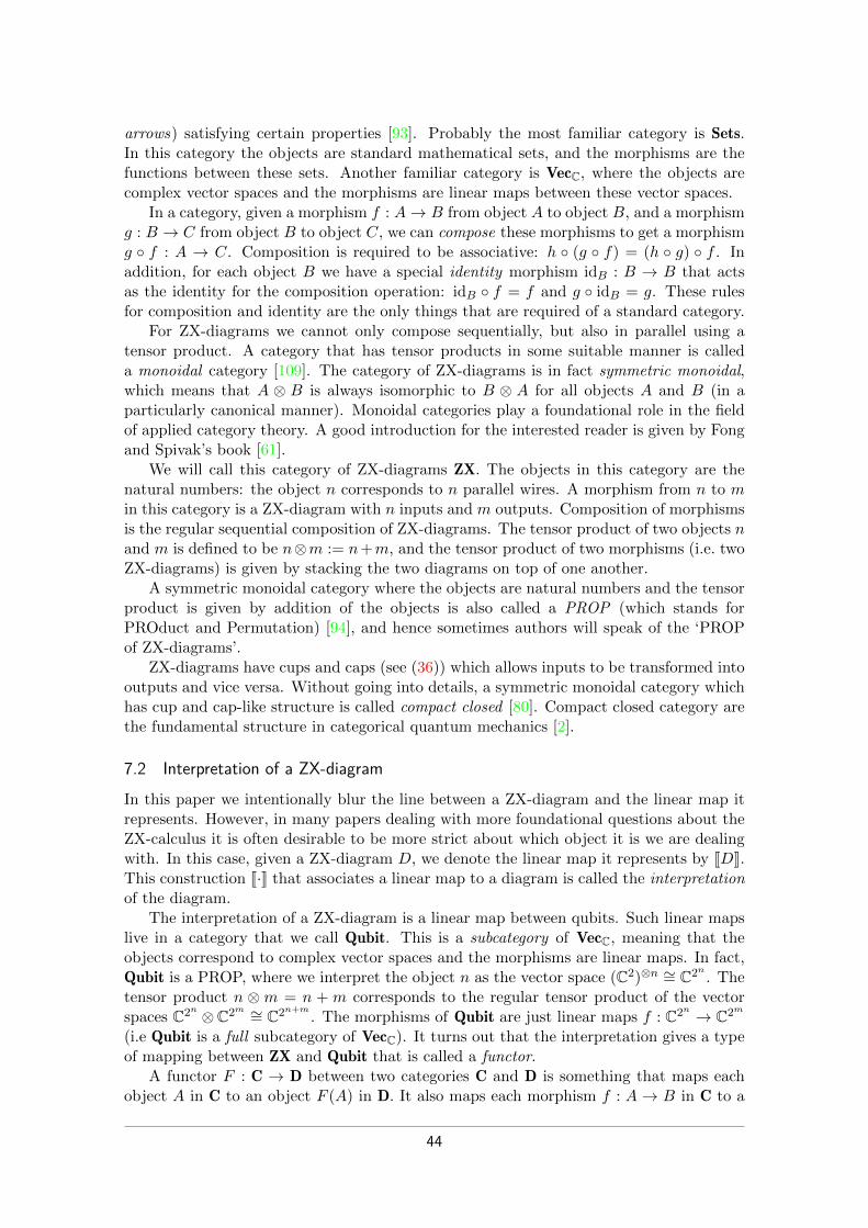
arrows) satisfying certain properties [93]. Probably the most familiar category is Sets.In this category the objects are standard mathematical sets, and the morphisms are thefunctions between these sets. Another familiar category is VecC, where the objects arecomplex vector spaces and the morphisms are linear maps between these vector spaces.
In a category, given a morphism f : A→ B from object A to object B, and a morphismg : B → C from object B to object C, we can compose these morphisms to get a morphismg ◦ f : A → C. Composition is required to be associative: h ◦ (g ◦ f) = (h ◦ g) ◦ f . Inaddition, for each object B we have a special identity morphism idB : B → B that actsas the identity for the composition operation: idB ◦ f = f and g ◦ idB = g. These rulesfor composition and identity are the only things that are required of a standard category.
For ZX-diagrams we cannot only compose sequentially, but also in parallel using atensor product. A category that has tensor products in some suitable manner is calleda monoidal category [109]. The category of ZX-diagrams is in fact symmetric monoidal,which means that A ⊗ B is always isomorphic to B ⊗ A for all objects A and B (in aparticularly canonical manner). Monoidal categories play a foundational role in the fieldof applied category theory. A good introduction for the interested reader is given by Fongand Spivak’s book [61].
We will call this category of ZX-diagrams ZX. The objects in this category are thenatural numbers: the object n corresponds to n parallel wires. A morphism from n to min this category is a ZX-diagram with n inputs and m outputs. Composition of morphismsis the regular sequential composition of ZX-diagrams. The tensor product of two objects nand m is defined to be n⊗m := n+m, and the tensor product of two morphisms (i.e. twoZX-diagrams) is given by stacking the two diagrams on top of one another.
A symmetric monoidal category where the objects are natural numbers and the tensorproduct is given by addition of the objects is also called a PROP (which stands forPROduct and Permutation) [94], and hence sometimes authors will speak of the ‘PROPof ZX-diagrams’.
ZX-diagrams have cups and caps (see (36)) which allows inputs to be transformed intooutputs and vice versa. Without going into details, a symmetric monoidal category whichhas cup and cap-like structure is called compact closed [80]. Compact closed category arethe fundamental structure in categorical quantum mechanics [2].
7.2 Interpretation of a ZX-diagramIn this paper we intentionally blur the line between a ZX-diagram and the linear map itrepresents. However, in many papers dealing with more foundational questions about theZX-calculus it is often desirable to be more strict about which object it is we are dealingwith. In this case, given a ZX-diagram D, we denote the linear map it represents by JDK.This construction J·K that associates a linear map to a diagram is called the interpretationof the diagram.
The interpretation of a ZX-diagram is a linear map between qubits. Such linear mapslive in a category that we call Qubit. This is a subcategory of VecC, meaning that theobjects correspond to complex vector spaces and the morphisms are linear maps. In fact,Qubit is a PROP, where we interpret the object n as the vector space (C2)⊗n ∼= C2n . Thetensor product n ⊗m = n + m corresponds to the regular tensor product of the vectorspaces C2n ⊗C2m ∼= C2n+m
. The morphisms of Qubit are just linear maps f : C2n → C2m
(i.e Qubit is a full subcategory of VecC). It turns out that the interpretation gives a typeof mapping between ZX and Qubit that is called a functor.
A functor F : C → D between two categories C and D is something that maps eachobject A in C to an object F (A) in D. It also maps each morphism f : A → B in C to a
44

morphism F (f) : F (A)→ F (B) in D. A functor is required to map identities to identities,F (idA) = idF (A), and to preserve composition, F (g ◦f) = F (g)◦F (f). For example, thereis the functor U : VecC → Sets that sends a vector space V to the set U(V ) = V anda linear map f : V → W to the same function U(f) = f . This functor essentially doesnothing except change the context in which we view the objects and morphisms. Such afunctor is known as a forgetful functor.
The interpretation of a ZX-diagram is a functor J·K : ZX→ Qubit. The objects of bothZX and Qubit are the natural numbers and we simply set JnK = n for all n ∈ N. As themorphisms of ZX are precisely ZX-diagrams, we set JDK to be the linear map the diagramD implements. We need to check that JidnK = idn and that JD ◦D′K = JDK◦JD′K, but thisis immediate from how we defined the interpretation of a ZX-diagram iteratively startingfrom the atomic generators. Note that we also have JD ⊗D′K ∼= JDK ⊗ JD′K, i.e. thatthe tensor product of diagrams corresponds to the tensor product of the underlying linearmaps. This makes J·K into a strong monoidal functor.
In Section 3.7 we showed that for any linear map between qubits we can find a ZX-diagram that represents it, i.e. that the ZX-calculus is universal. In terms of the interpre-tation functor J·K we can phrase this as stating that for any morphism f : C2n → C2m inQubit we can find a morphism D : n→ m in ZX such that JDK = f . A functor which hasthis property, which is reminiscent of the surjectivity of a function, is called full.
7.3 Rewriting and completenessIn the previous subsection we saw that universality of the ZX-calculus corresponds tofullness of the interpretation functor. For a functor, being full is what being surjectiveis to a function. An immediate question is then: what about injectivity? An ‘injective’functor is called faithful : for a faithful functor F : C → D an equality F (f : A → B) =F (g : A→ B) implies f = g.
The functor J·K : ZX → Qubit is not faithful. This is because there are multipledifferent ZX-diagrams that represent the same linear map. This of course does not comeas a surprise as we have been constantly rewriting ZX-diagrams with the promise that thelinear maps they represent are the same.
The solution to this ‘problem’ is to consider a modified category ZX/∼ where ZX-diagrams that can be transformed into one another by the rewrite rules of Figure 1 areidentified with one another. The way to do this is to consider the smallest equivalencerelation ∼ with the following properties:
• D1 ∼ D2 for each of the equalities D1 = D2 in Figure 1.
• If D1 ∼ D2, then also (E ◦ D1 ◦ C) ∼ (E ◦ D2 ◦ C) for all diagrams C and E. Inother words: if two diagrams are equivalent, then they remain equivalent when someother diagrams are composed with them.
• If D1 ∼ D2, then also (E ⊗D1 ⊗ C) ∼ (E ⊗D2 ⊗ C) for all diagrams C and E.
These rules for the equivalence relation ∼ correspond precisely to how we have been usingZX-calculus rewrite rules intuitively in the previous sections.
We can now define the morphisms of ZX/∼ to be equivalence classes [D]/∼ of diagramsunder the relation ∼. Using the properties of ∼ above it is straightforward to verify that[D1]/∼ ◦ [D2]/∼ := [D1 ◦D2]/∼ gives a well-defined composition of these classes. We cansimilarly define a tensor product, and hence ZX/∼ is again a PROP.
For the interpretation functor J·K : ZX/∼ → Qubit we wish to setq[D]/∼
y:= JDK. For
this to be well-defined we need the value of JDK to not depend on the representative of the
45
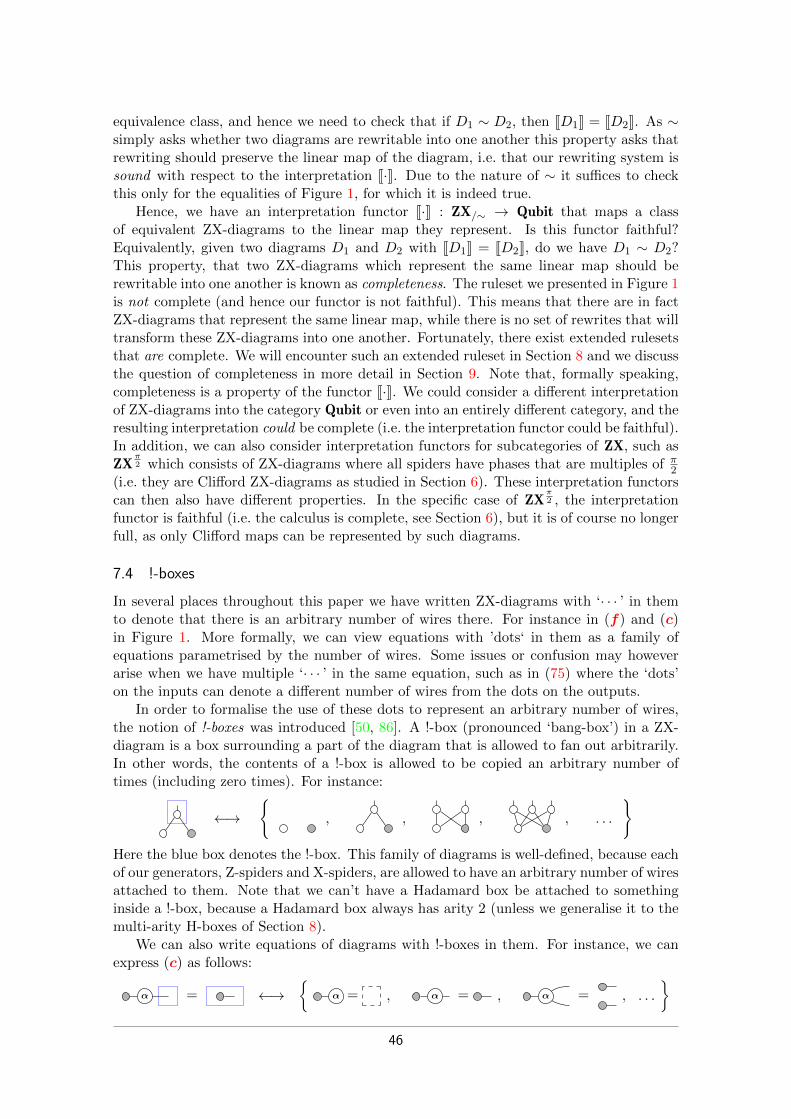
equivalence class, and hence we need to check that if D1 ∼ D2, then JD1K = JD2K. As ∼simply asks whether two diagrams are rewritable into one another this property asks thatrewriting should preserve the linear map of the diagram, i.e. that our rewriting system issound with respect to the interpretation J·K. Due to the nature of ∼ it suffices to checkthis only for the equalities of Figure 1, for which it is indeed true.
Hence, we have an interpretation functor J·K : ZX/∼ → Qubit that maps a classof equivalent ZX-diagrams to the linear map they represent. Is this functor faithful?Equivalently, given two diagrams D1 and D2 with JD1K = JD2K, do we have D1 ∼ D2?This property, that two ZX-diagrams which represent the same linear map should berewritable into one another is known as completeness. The ruleset we presented in Figure 1is not complete (and hence our functor is not faithful). This means that there are in factZX-diagrams that represent the same linear map, while there is no set of rewrites that willtransform these ZX-diagrams into one another. Fortunately, there exist extended rulesetsthat are complete. We will encounter such an extended ruleset in Section 8 and we discussthe question of completeness in more detail in Section 9. Note that, formally speaking,completeness is a property of the functor J·K. We could consider a different interpretationof ZX-diagrams into the category Qubit or even into an entirely different category, and theresulting interpretation could be complete (i.e. the interpretation functor could be faithful).In addition, we can also consider interpretation functors for subcategories of ZX, such asZX
π2 which consists of ZX-diagrams where all spiders have phases that are multiples of π
2(i.e. they are Clifford ZX-diagrams as studied in Section 6). These interpretation functorscan then also have different properties. In the specific case of ZX
π2 , the interpretation
functor is faithful (i.e. the calculus is complete, see Section 6), but it is of course no longerfull, as only Clifford maps can be represented by such diagrams.
7.4 !-boxesIn several places throughout this paper we have written ZX-diagrams with ‘· · · ’ in themto denote that there is an arbitrary number of wires there. For instance in (f) and (c)in Figure 1. More formally, we can view equations with ’dots‘ in them as a family ofequations parametrised by the number of wires. Some issues or confusion may howeverarise when we have multiple ‘· · · ’ in the same equation, such as in (75) where the ‘dots’on the inputs can denote a different number of wires from the dots on the outputs.
In order to formalise the use of these dots to represent an arbitrary number of wires,the notion of !-boxes was introduced [50, 86]. A !-box (pronounced ‘bang-box’) in a ZX-diagram is a box surrounding a part of the diagram that is allowed to fan out arbitrarily.In other words, the contents of a !-box is allowed to be copied an arbitrary number oftimes (including zero times). For instance:
←→{
, , , , . . .
}Here the blue box denotes the !-box. This family of diagrams is well-defined, because eachof our generators, Z-spiders and X-spiders, are allowed to have an arbitrary number of wiresattached to them. Note that we can’t have a Hadamard box be attached to somethinginside a !-box, because a Hadamard box always has arity 2 (unless we generalise it to themulti-arity H-boxes of Section 8).
We can also write equations of diagrams with !-boxes in them. For instance, we canexpress (c) as follows:
α = ←→{
α = , α = , α = , . . .
}
46

The dashed box in the first equation denotes an empty diagram, corresponding to the!-box being expanded zero times.
Some rules require more than one !-box to be expressed. For instance, the generalisedbialgebra equation (75) can be expressed as follows:
= (107)
When writing an equation involving !-boxes it is important that the !-boxes on the left-hand side are matched 1-to-1 to those on the right-hand side. In (107) it is clear that theleft !-boxes of each side of the equation match, because otherwise the equations would notbe well-typed (they would have a different number of inputs). Formally, we would have togive a ‘name’ to each !-box so that it is clear which corresponds to which on each side ofthe equation. In practice, it is often clear how they correspond by their positioning in thediagram. Consider for instance the spider fusion rule (f) expressed using multiple !-boxes:
β
α
=α+β
(108)
!-boxes can also overlap and be nested (but note that when nested in a rule, they mustbe nested in the same way on both sides of the equation). For instance, we can express (aspecial case of) the pivot simplification rule (103) using !-boxes as follows:
= (109)
Note that not all repeated structure can be expressed using !-boxes. For instance, theiterated application of a linear map, or the notion of a fully connected graph as in (102).13
!-boxes are used in the software Quantomatic [85] in order to express families of dia-grammatic rewrite rules. While !-boxes are not necessary for many manual derivations,they do sometimes become essential for expressing particularly complicated families ofrewrite rules. For instance, normal form diagrams in the ZH-calculus [11] are naturallyexpressed using a variation on !-boxes called annotated !-boxes, where a !-box is labelledby an element from some finite set and elements inside the !-box are allowed to use thiselement as a variable. Complicated rewrite rules such as the graphical Fourier transform,cf. Section 8.4 or [89], or the hyper-pivot rule [91] also require (annotated) !-boxes to beexpressed concisely.
7.5 Monoids, comonoids, Frobenius algebras and bialgebrasThe central generators of ZX-diagrams, the spiders, have an algebraic structure that isused far beyond just the ZX-calculus. In this section we will give some definitions regardingthis structure, each building on the previous.
One of the most basic algebraic structures is the monoid. A monoid is a set M with abinary operation · that is associative, a ·(b ·c) = (a ·b) ·c, and has a unit, 1 ·a = a = a ·1. Ina monoidal category we can view a monoid as a pair of morphisms µ : M ⊗M →M andν : I →M satisfying µ◦(µ⊗ idM ) = µ◦(idM ⊗µ) and µ◦(ν⊗ idM ) = idM = µ◦(idM ⊗ν).
13This first issue can be fixed through the definition of a different type of box as suggested in [97].For (102) specifically, the issue of a fully connected graph can be sidestepped by viewing Hadamard boxesas H-edges so that they can cross into !-boxes. A fully connected graph can then be represented by a vertexinside a !-box with an H-box looping to the same vertex that goes outside the !-box.
47

Here µ represents the multiplication operation, and ν points towards the identity in M (Ihere is the monoidal unit of the category, A⊗ I ∼= A for all A). We can form a monoid inZX where M = 1 by using the Z-spider:
µ = ν = (110)
The associativity and unit conditions are then given by spider fusion:
= =
= = =(111)
In fact, this is a commutative monoid, since:
= (112)
Of course nothing here is particular to the Z-spider, and this also works for the X-spider.A notion that is perhaps less familiar, but still equally fundamental is the comonoid.
Whereas a monoid takes two elements of M and outputs a single element of M , a comonoiddoes the opposite, taking a single element and outputting two. Note that, in general, theword ‘co’ in category theory denotes that you should take the dual definition which isgiven by switching the direction of all the morphisms involved. In terms of our diagramsthis corresponds to horizontally flipping the diagram. Concretely, a comonoid consists ofmaps δ : M → M ⊗M and ε : M → I that satisfy (δ ⊗ idM ) ◦ δ = (idM ⊗ δ) ◦ δ and(ε⊗ idM ) ◦ δ = idM = (idM ⊗ ε) ◦ δ. The map δ is called the co-multiplication, while ε iscalled the co-unit. Again, the Z-spider forms an example of this:
δ = ε = (113)
And the co-associativity and co-unit equations are again proven using spider fusion:
==
===(114)
Analogous to (112), this comonoid is co-commutative.We now see that the basic Z-spiders of arity 1 and arity 3 form a monoid and a
comonoid. This monoid and comonoid structure of the Z-spider interact in a particularlynice way that makes the Z-spider a Frobenius algebra.14. A Frobenius algebra is a monoidtogether with a comonoid that satisfy the Frobenius conditions:
= = (115)
14Frobenius algebras have a long history. The name itself was coined in 1941 [98], with the first categoricaldefinition given in 1969 [90]. For a good modern reference see [114] or the monograph [87]. The first useof Frobenius algebras in describing structure in quantum theory was in 2008 [32]
48

As the monoid and comonoid of the Z-spider are (co-)commutative, the structure we getis actually a commutative Frobenius algebra. Additionally, the Z-spider also satisfies thefollowing equation:
= (116)
Frobenius algebras satisfying these conditions are called special. The Z-spiders hence forma commutative special Frobenius algebra. This Frobenius algebra has one more importantproperty that will require some further definitions.
In the category of ZX-diagrams ZX or the category of finite-dimensional complex vectorspaces fVecC we have a way of ‘flipping’ a morphism f : A→ B to a morphism f † : B → A.Namely, by taking the adjoint of the linear map in the latter case, and flipping a ZX-diagram horizontally and changing the signs of all the phases in the former case. This †operation satisfies 3 properties of interest: it is involutive, (f †)† = f , it is contravariant,(f ◦ g)† = g† ◦ f †, and it is the identity on objects, A† = A. A category that has anoperation with these properties is called a dagger-category [108].
For the Z-spider, the monoid µ and the comonoid δ are related by the dagger: µ† = δ.Similarly, the unit ν and counit ε are also related via ν† = ε. A Frobenius algebra on adagger-category where the monoid and comonoid are related in this manner is called adagger-Frobenius algebra.
So to summarise: the Z-spiders form a commutative special dagger-Frobenius algebra.Our entire discussion also holds for the X-spiders, and in fact holds for any family of mapssatisfying a version of the spider fusion rule (f) and the identity rule (id). It turns out thata converse statement is also true [38]: if we have a commutative special dagger-Frobeniusalgebra on a finite-dimensional complex vector space V , then there exists an orthonormalbasis |v1〉 , . . . |vn〉 of V such that the Frobenius algebra is given by the spiders
...
... =
n∑i=1|vi · · · vi〉〈vi · · · vi| , (117)
analogously to the definition of the Z-spider in (21). Another way we can view this resultis that the spider equation (f) essentially gives a diagrammatic characterisation of thenotion of an orthonormal basis.
The Frobenius algebra structure characterises a single spider, either Z or X. The inter-action between the two species of spiders is however also a special case of a well-studiedstructure. A bialgebra consists of a monoid (that we will suggestively write as the Z-spider)and a comonoid (that we write as the X-spider) satisfying the following equations:
==
= =
(118)
Here the dashed box represents an empty diagram. The Z-spider and X-spider evidentlyform a bialgebra15; see (c) and (b). As was the case for the Frobenius structure, they donot just form a bialgebra. As the monoid and comonoid structure are (co-)commutativewe can call this a commutative bialgebra, but there is some additional structure. Given a
15In a bialgebra these equations hold on the nose, while in the ZX-calculus they only hold up to scalar.Such a structure might more accurately be called a scaled bialgebra.
49

bialgebra on an object M , an antipode is a map a : M →M that satisfies the Hopf law :
=a
a= (119)
A bialgebra that has an antipode is called a Hopf algebra. The Z-spider and X-spider forma Hopf algebra where the antipode is equal to the identity, as is evident from (72).
We chose the Z-spider to supply the monoid and the X-spider to supply the comonoid,but we could have chosen to do this the other way around. A pair of Frobenius algebrasthat is a Hopf algebra in these two ways is variously called a pair of interacting Frobeniusalgebras [52], interacting Hopf algebras [17], interacting bialgebras [16] or a Hopf-Frobeniusalgebra [40].
Much of what we said in this section can generalise to linear maps on higher-dimensionalspaces (in contrast to the two-dimensional spaces we have been working with). We discussqudits in more detail in Section 10.3.
8 Toffoli gates and the ZH-calculusIn our discussion on the ZX-calculus in Sections 2–6 we have focused on gate sets consistingof single-qubit gates combined with the CNOT gate. This however skips over other widelyused multi-qubit gates, in particular Toffoli gates and other multiply-controlled gates.While the ZX-calculus is very useful when it comes to reasoning about circuits based onCNOT gates and related gates like the CZ or the Ising-type unitaries such as the phasegadget of Section 5.6, it is considerably harder to work with multiply-controlled gates.This can be pinpointed to the fact that there is no concise way to represent the ANDoperation on computational basis states |x〉⊗ |y〉 7→ |x · y〉. Note that the important wordhere is ‘concise’. As ZX-diagrams are universal (cf. Section 3.7) any linear map can berepresented, but not always in a useful manner.
In this section we will discuss a variation on the ZX-calculus that is called the ZH-calculus. This was introduced in 2018 by Backens and Kissinger [11] and introduces a newgenerator, the H-box, that generalises the Hadamard box we have been using to arbitraryarity, and which allows an easy representation of Toffoli gates and other multiply-controlledgates. Though the ZH-calculus was introduced as an alternative calculus, we will treat ithere simply as an extension of the ZX-calculus that allows us to efficiently reason about alarger class of diagrams.16
First, in Section 8.1 we introduce H-boxes. Then in Section 8.2 we introduce theadditional rewrite rules that allow us to reason about this generator. As a demonstrationof its utility, we use H-boxes in Section 8.3 to construct the graphical representation ofseveral controlled unitaries. Then in Section 8.4 we recall the Fourier transform of semi-Boolean functions in order to relate H-boxes to Z- and X-spiders and the phase polynomialsof Section 5.6. Finally, in Section 8.5 we prove diagrammatically some known optimisationsof Toffoli gates using H-boxes and the Fourier transform.
8.1 H-boxesAs discussed above, using Z- and X-spiders, there is no concise way to represent thecoherent AND gate that maps the computational basis state |x〉 ⊗ |y〉 to |x · y〉. If we had
16The H-box is not the only way to simplify the representation of Toffoli gates in the ZX-calculus.Another approach is given by introducing the ‘triangle’ generator that we will encounter in Section 9.3.
50

such an AND gate, we could implement a Toffoli gate as follows:
AND
(120)
Indeed, inputting computational basis states into the top two qubits we calculate:
xπ
yπ
AND=
xπ
yπANDxπ
yπ(c)
=
xπ
yπ
(x · y)π =
xπ
yπ
(x · y)π
(f)(121)
Hence, this construction ‘activates’ a NOT gate on the bottom qubit when the top twoqubits are in the |1〉 state. This is exactly the action |x, y, z〉 7→ |x, y, (x · y)⊕ z〉 of theToffoli gate.
As discussed in Section 4.5, the Z-spider implements a coherent COPY gate whenacting on computational basis states, and the X-spider implements an XOR. We mightthen hope that we could add another spider that implements the AND gate. However,one of the main symmetries present in the Z- and X-spiders does not hold for the ANDgate (which can be verified by calculating the associated matrices):
AND 6= AND= but (122)
It is however possible to ‘split up’ the AND gate into two components, each of which dohave all the symmetries that the spiders have. We call these components H-boxes, forreasons that will become clear, and they are defined as follows:
a nm ...
... :=
∑ai1...imj1...jn |j1 . . . jn〉 〈i1 . . . im| (123)
The sum in this equation is over all i1, . . . , im, j1, . . . , jn ∈ {0, 1} and a is an arbitrarycomplex number. Hence, an H-box represents a matrix with all entries equal to 1, exceptthe bottom right element, which is equal to a. We have for instance
a =(
1 1 1 11 1 1 a
)and a =
(1 11 a
). (124)
Hence, in particular, when a = −1, the 1-input 1-output H-box is just a rescaled Hadamard:
= 1√2−1 (125)
The H-boxes are thus a generalisation of Hadamard gates to an arbitrary number of inputsand outputs (hence, the letter ‘H’). Just as spiders with a zero phase are depicted withouta phase label, we will depict H-boxes with a label of −1 without any label:
...
...
nm := ...−1...
nm (126)
51

This convention means that the 1-input 1-output H-box with a phase of −1 is denotedexactly the same as the Hadamard gate in the ZX-calculus. As these two diagrams repre-sent the same matrix up to a scalar factor of 1√
2 this is fine as long as one does not care
about the exact scalar value. Where this matters we will denote which definition we areusing. In this section we will use the definition of H-boxes of (123).
The linear maps that H-boxes represent have all the symmetries we would expect froma spider:
a==a a = aa... =... ...
......
......
... ... ... ... ...
Now, as promised, the H-boxes are indeed the components with which we can constructthe coherent AND:
=(
2 2 2 00 0 0 2
)= 2 AND (127)
We can then easily write down the Toffoli gate:
(128)
This simple representation of the AND (requiring just two diagrammatic generators) allowsus to efficiently diagrammatically reason about constructions involving the AND, as wewill see in the next section.
8.2 The ZH-calculusThe reason we care about H-boxes is because they come equipped with a new set of rewriterules called the ZH-calculus. These rewrite rules can essentially be grouped into two sets.The rules in the first set are motivated by the relationship of the H-boxes to the ANDgate, while the second section contains rules that relate H-boxes with different labels.
While ostensibly part of the second set, let us first note the following fundamentalrelation between an arity-1 H-box and a Z-spider:
eiα = α (129)
In particular, taking respectively α = 0 and α = π, we get:
1 = = π (130)
To understand the first set of rules it will be helpful to use multi-input AND gates:
AND... = ... (131)
A rule on H-boxes we have already seen is that two Hadamard gates cancel, cf. (14). Usingour interpretation of multi-input AND gates (131) using H-boxes we can gain a differentview on this equation. Indeed, using (131) we see that two Hadamard gates in a rowcorrespond to an AND gate with a single input, and this gate is of course the identity.
52

The first new rule expresses how a sequence of ANDs can be combined into a singlemulti-input AND:
AND...
AND...
=AND
...
...
↔
...
...
=
......
(132)This rule can be presented a bit more generally as an H-box fusion rule:
a...
a =...
...
... (133)
An important consequence of this rule is that H-boxes absorb |1〉 states:
...
π a =(h)
...
π a =(130)
...
a =(133)
...
a (134)
We will see later in (138) that, in contrast, a |0〉 ‘explodes’ an H-box.In Section 4.5 we saw how the interpretation of the Z- and X-spider as respectively
COPY and XOR lead us to the bialgebra rule that allowed us to push (phaseless) Z- andX-spiders through each other. This equation (65) involving COPY and XOR holds inexactly the same way when XOR is replaced by AND:
=COPYAND
COPY
COPY AND
AND
(135)
We can directly translate this into a rule involving Z-spiders and H-boxes:
=···
···
nm ···
···
nm (136)
By pushing the Hadamard through the Z-spider and cancelling some Hadamards we canalso present this in a format that is often more convenient:
=···
···
nm ···
···
nm (137)
As in (75), the right-hand side of both of these equations is a fully connected bipartitegraph. Note that as a special case of the second equation (taking n = 0) we get thefollowing useful state copy rule, which is a counterpart of (134):
a =···
···
···=
a
···
a
=(133) (137)
(138)
Here in the last step we dropped the scalar subdiagram, as it only contributes a (usuallyirrelevant) non-zero scalar.
Another consequence of this bialgebra rule is that the identification of a 1-labelledH-box with a Z-spider of (130) can be generalised to higher arity as follows:
=1
. . . (133) . . .
1
=(130) . . . (63) . . .
=(138) . . .
= (139)
53

=
a...
a =...
...
...
=···
···
···
···
=
1
π
=
=
Figure 2: The phase-free rules of the ZH-calculus.
Let us now introduce the last pair of AND-inspired rewrite rules for H-boxes. Theseare based on the following identities:
AND = AND π =π
π(140)
The first is quite self-evident: if we copy a value and then AND those values together, it isthe same thing as doing nothing to the value. The second requires a bit more explanation.It expresses a fact about the possible ways that AND can return |1〉. Indeed, as a linearmap, we can write AND as |0〉〈00| + |0〉〈01| + |0〉〈01| + |1〉〈11|, and hence post-selectingthe output of AND with 〈1| we calculate 〈1|AND = 〈11|.
Writing the ANDs as H-boxes and simplifying the expressions a bit we get the followingrewrite rules17:
= π =π
π(141)
Note that using (130) we could also have written the second equation of (141) as:
= (142)
The rules introduced so far are summarised in Figure 2.We have now covered all the ‘AND inspired’ ZH-calculus rules. In fact, these rules,
together with some of the ZX-calculus rules of Figure 1, are complete for the Hadamard-Toffoli fragment of the ZH-calculus [115], where phases on spiders are limited to 0 and πand H-boxes can only be labelled by the default −1. This means that when we have twocircuits (or more generally, arbitrary diagrams) that represent the same linear map andthat consist solely of Hadamard and Toffoli gates, then by representing these diagramsusing spiders and H-boxes and using just the rules of Figure 1 and 2 we can prove diagram-matically that they are equal.18 This is significant because Hadamard+Toffoli circuits areapproximately universal for quantum computation [3, 111]. Hence, unlike the rules ofFigure 1 that are only complete for the Clifford fragment, we could in principle use therules we have covered up to this point to do arbitrary calculations for the approximatelyuniversal model of quantum computation given by the Toffoli+Hadamard gate set.
The second set of rules of the ZH-calculus has to do with how labelled H-boxes interact.The first two of these rules allow us to perform arithmetic with H-boxes:
b
a= ab
a
b= a+b
2π (143)
17These rules were not present as axioms in the original ZH-calculus paper [11]. Instead, they follow asconsequences of their (O) rule, which is arguably harder to motivate and to use. It is possible to prove(O) using the rules of (141), and so in that sense they are equivalent [14].
18The complete ruleset presented in [115] is somewhat different from the one we present. That the rulesetwe present is complete is shown in a forthcoming paper [14].
54

These rules are known as the ‘multiply rule’ and the ‘average rule’ [11]. When a and b arecomplex phases, the multiply rule is just an instance of the adding of phases when spidersfuse, cf. (129) and (48). The average rule has no counterpart in the standard ZX-calculus.In practice, the average rule doesn’t turn out to be useful very often. We include it heremerely for completeness’ sake.
The multiply rule can be generalised to H-boxes of arbitrary arity:
a
b= ab..
.
... (144)
I.e. when two H-boxes are connected to exactly the same set of Z-spiders, then we can fusethe H-boxes together. With the rules we have seen before, the proof of this generalisationis straightforward:
a
b= ab. . . . . .. . .=
a
b
(133)=
a
b
(136). . . = ab
(143). . .
(133)(145)
This rule appears quite often in the form where a = b = −1, so that ab = 1 and the H-boxdecomposes into white spiders according to (139). As an example, we can use this rule toprove that two Toffoli gates reduce to the identity:
=
(h)=
(hh)(f)
=(144)
1=
(139)=
(f)(id)
(hh)(146)
Then there is only one more rule: the introduction rule:
a
a=
π
a (147)
It is called the introduction rule, because it allows you to introduce additional edges to anH-box (at the cost of copying the H-box). As do many of the previously introduced rules,it has a generalisation to H-boxes of arbitrary arity:
a
a=
π
a ...
... (148)
Most of the use-cases of this rule are when it is applied from right-to-left. Indeed, it is aclose cousin of the multiply rule (144). Both rules target pairs of H-boxes connected to thesame set of Z-spiders, although in the case of the introduction rule, they must also differby a NOT gate on one of the connections, and have the same label. As an example, wecan use the introduction rule to prove that if we apply both a controlled-phase gate, anda NOT-conjugated controlled-phase gate that this reduces to just a simple phase gate:
=
(π)
eiα eiα
π π (f)
eiα eiαπ
=(147)
eiα=
(id)
α
(129)
α =
(f)(149)
As noted above, the ‘AND inspired’ rules together with the ZX-calculus rules are com-plete for diagrams generated by Toffoli and Hadamard gates. When we add these three
55

additional rules, multiply, average and introduction, we get a rule set that is complete forall diagrams [11]. The ZH-calculus, being a superset of the ZX-calculus, is also universal.Hence, we can, in principle, replace all reasoning about qubit linear maps with diagram-matic reasoning. Whether it is beneficial to do so of course depends on the situation.
8.3 Controlled unitariesA useful feature of the ZH-calculus is that it allows us to quite easily see how to make acontrolled-unitary out of a unitary given as a ZH-diagram. This is perhaps most easilydemonstrated by the difference between a CZ and a CCZ gate in the ZH-calculus:
CZ = CCZ = (150)
This suggests a general procedure for adding a control qubit: identify which H-box ‘acti-vates’ the application of your gate, and add another wire to it which connects to a Z-spideron your control qubit. Sometimes, one has to work a bit to uncover the correct H-box.For instance, to see how a Z gate relates to a CZ, we unfuse its phase:
π =
(f) π
=(130)
(151)
This procedure also works for making controlled-phase gates if the phase is somethingother than π:
CZ(α) = eiα (152)
For diagrams containing X-spiders we will usually have to convert these to Z-spiders using(h) in order to see where we should add the control wire. For instance, to go from a CNOTto a CCNOT (Toffoli):
=
(h) =
(h)(153)
Note that we here added a control wire to the ‘middle’ H-box, but left the Hadamardson the qubit wire alone. This is a general rule for constructing a controlled diagram. Forinstance, it might be tempting to define a controlled-Hadamard as follows:
(154)
While this does indeed implement a Hadamard gate when the control qubit is in the |1〉state (although with the wrong normalisation), it does not reduce to the identity whenthe control qubit is |0〉:
=
(c)=
(138)(155)
To construct the actual controlled-Hadamard we need to find the ‘hidden’ H-boxes in theHadamard gate. The way we do this is by using its decomposition into Euler angles:
= π2
π2
π2e−i
π4 (156)
56
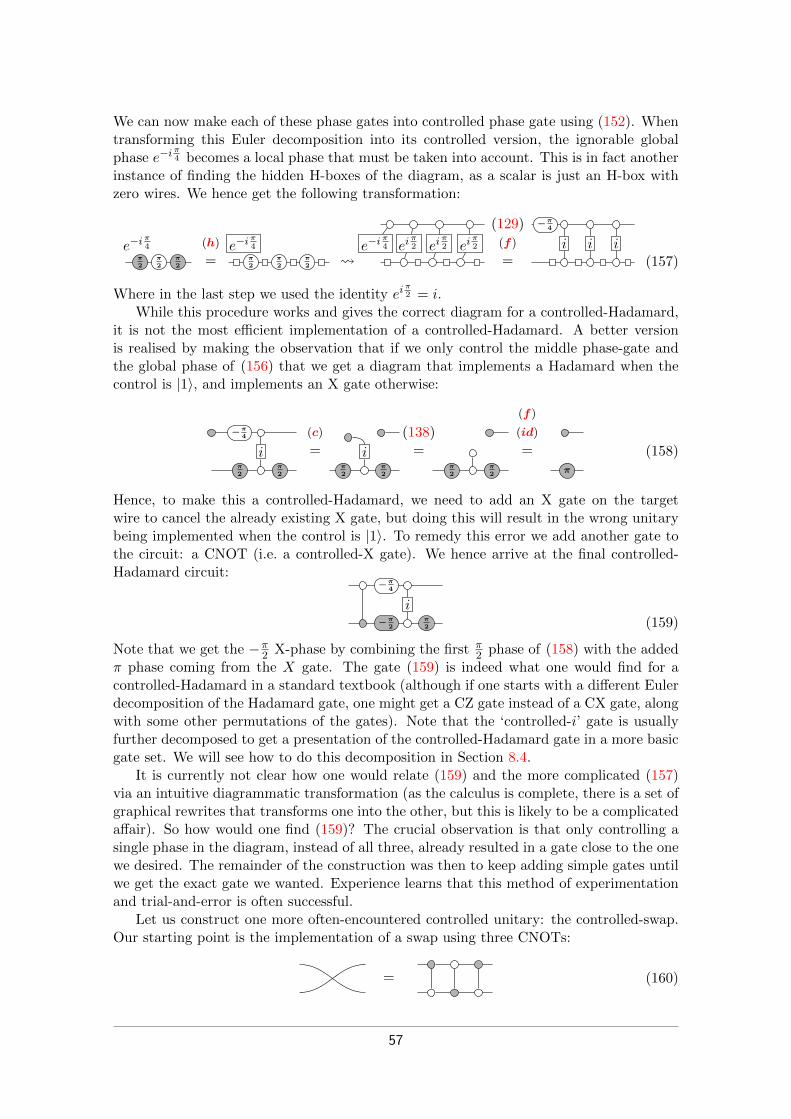
We can now make each of these phase gates into controlled phase gate using (152). Whentransforming this Euler decomposition into its controlled version, the ignorable globalphase e−i
π4 becomes a local phase that must be taken into account. This is in fact another
instance of finding the hidden H-boxes of the diagram, as a scalar is just an H-box withzero wires. We hence get the following transformation:
π2
π2
π2
e−iπ4
=
(h)π2
π2
π2
e−iπ4
e−i
π4 ei
π2 ei
π2 ei
π2
=
−π4
i i i
(129)(f)
(157)
Where in the last step we used the identity eiπ2 = i.
While this procedure works and gives the correct diagram for a controlled-Hadamard,it is not the most efficient implementation of a controlled-Hadamard. A better versionis realised by making the observation that if we only control the middle phase-gate andthe global phase of (156) that we get a diagram that implements a Hadamard when thecontrol is |1〉, and implements an X gate otherwise:
=π2
π2
−π4
i
(c)
π2
π2
i =(138)
π2
π2
=
(f)
π
(id)(158)
Hence, to make this a controlled-Hadamard, we need to add an X gate on the targetwire to cancel the already existing X gate, but doing this will result in the wrong unitarybeing implemented when the control is |1〉. To remedy this error we add another gate tothe circuit: a CNOT (i.e. a controlled-X gate). We hence arrive at the final controlled-Hadamard circuit:
−π2
π2
−π4
i(159)
Note that we get the −π2 X-phase by combining the first π
2 phase of (158) with the addedπ phase coming from the X gate. The gate (159) is indeed what one would find for acontrolled-Hadamard in a standard textbook (although if one starts with a different Eulerdecomposition of the Hadamard gate, one might get a CZ gate instead of a CX gate, alongwith some other permutations of the gates). Note that the ‘controlled-i’ gate is usuallyfurther decomposed to get a presentation of the controlled-Hadamard gate in a more basicgate set. We will see how to do this decomposition in Section 8.4.
It is currently not clear how one would relate (159) and the more complicated (157)via an intuitive diagrammatic transformation (as the calculus is complete, there is a set ofgraphical rewrites that transforms one into the other, but this is likely to be a complicatedaffair). So how would one find (159)? The crucial observation is that only controlling asingle phase in the diagram, instead of all three, already resulted in a gate close to the onewe desired. The remainder of the construction was then to keep adding simple gates untilwe get the exact gate we wanted. Experience learns that this method of experimentationand trial-and-error is often successful.
Let us construct one more often-encountered controlled unitary: the controlled-swap.Our starting point is the implementation of a swap using three CNOTs:
= (160)
57

We could make this controlled by transforming each of the CNOTs into a Toffoli. However,just as with the controlled-Hadamard, we realise that if we ‘deactivate’ the middle CNOT,that the outer CNOTs cancel each other, and hence it suffices to add a control to the middleCNOT. We can diagrammatically simplify the resulting gate:
=
(b)(f)
=
(b)(f)
=
(72)= (161)
In the final diagram, if the control qubit is in the |1〉 state, we can ignore the control wire(because the |1〉 is absorbed as in (134)). The resulting diagram then has the shape of thebutterfly network commonly used in the literature on linear network coding [15, 45]. Inthis case, the two resulting Hadamards in the middle cancel out, and by inputting statesthis can easily be verified to implement a swap. On the other hand, if the control is |0〉,the 3-ary H-box disconnects (cf. (138)), and the diagram collapses to the identity.
8.4 The graphical Fourier transformAs was shown in Section 3.7, the ZX-calculus is universal, meaning that any linear mapbetween qubits can be represented as a ZX-diagram. This includes H-boxes. So how canan H-box be constructed using Z- and X-spiders? We have already seen a number of specialcases. In (129) we represented 1-ary H-boxes carrying a complex phase as a Z-spider. TheEuler decomposition of the Hadamard gate (44) gives a translation for a 2-ary H-box withphase −1. In fact, a more useful translation turns out to be (45) as this generalises in astraightforward way to 2-ary H-boxes carrying an arbitrary complex phase:
eiα = α2
α2
−α2
(162)
This identity is already sufficient to decompose the controlled-phase gate that appearsin (159). To see where this identity comes from and how it generalises we need to introducethe notion of a Fourier transform of a semi-Boolean function.
A semi-Boolean function is a function f : Bn → R, where B = {0, 1} is the Booleans.We can write a semi-Boolean function as a sum of primitive terms in two useful ways. Thefirst way is to take the primitive function to be XOR:
f(~x) =∑~y∈Bn
λ~y(⊕
~y · ~x).
Here the λ~y are real coefficients that determine f , the ‘multiplication’ operation · is thecomponentwise multiplication of bitstrings, and
⊕denotes the XOR of all the bits in a
bitstring. Let us give an example. If ~y = 101, then⊕~y · ~x = x1 ⊕ x3. Note that in
this sum we are treating the Booleans 1 and 0 both as Booleans and as real numbers.This decomposition contains 2n independent parameters λ~y. As f has 2n possible inputs,we see that each semi-Boolean function can indeed uniquely be written in this way. Thephase polynomials we saw in Section 5.6 are examples of semi-Boolean functions writtenas XOR terms.
The second decomposition is to take the primitive function to be AND:
f(~x) =∑~y∈Bn
λ~y∏
~x~y.
58

Here ~x~y is the bitstring xy11 x
y22 · · ·xynn where we set 00 = 1 and 10 = 1. Hence, if ~y = 101
then ~x~y = x11x3, so that∏~x~y = x1 ∧ x3. Again, as there are 2n independent terms in
this decomposition, any semi-Boolean function can be written in this way.The transformation of a semi-Boolean function written as sums of XOR terms to one
written as sums of AND terms and back is what we call the Fourier transform of such afunction. As the X-spider allows us to compute the XOR of basis states, and the H-boxallows us to compute the AND, it should come as no surprise that this Fourier transformrelates these two generators.
This Fourier transform essentially boils down to one simple identity that holds forBoolean variables x and y:
x⊕ y = x+ y − 2(x · y) (163)
This equation allows us to write a 2-ary XOR term as a sum of AND terms. By iteratingit, we can also reduce higher-arity XOR terms:
(x⊕ y)⊕ z = x⊕ z + y ⊕ z − 2(x · y)⊕ z= x+ z − 2(x · z) + y + z − 2(y · z)− 2(x · y)− z + 4(x · y · z)= x+ y + z − 2(x · y + x · z + y · z) + 4(x · y · z)
We can also take the ‘inverse’ of (163):
x · y = 12(x+ y − x⊕ y) (164)
And again, this generalises:
x · y · z = 14(x+ y + z − x⊕ y − x⊕ z − y ⊕ z + x⊕ y ⊕ z) (165)
For an example of how this relates to quantum gates, let us consider a simple example.The action of a CZ gate on a computational basis state |xy〉 can be written as CZ |xy〉 =(−1)x·y |xy〉. Using (164) and −1 = eiπ we can then write (−1)x·y = ei
π2 (x+y−x⊕y). As
diagrams, the equality of these two representations becomes the following identity:
=π2
π2
−π2 (166)
I.e. on the left-hand side we see that the two input states get copied to the H-box in themiddle, which gives a −1 phase if both inputs are |1〉. On the right-hand side we seetwo S gates, that supply conditional phases ei
π2 x and ei
π2 y, while the central phase gadget
(see (86)), supplies e−iπ2 x⊕y. Note that this equality can be easily derived diagrammatically
from the decomposition of the Hadamard gate in (45). If instead of a CZ gate, we startedwith a CZ(α) gate (152), we would have end up with the decomposition (162).
This process works very similarly for the CCZ gate. Indeed, CCZ |xyz〉 = (−1)x·y·z |xyz〉,and hence, using (165), we expect the following equality:
=
π4
π4
π4
−π4
−π4
−π4
π4
(167)
This identity can be proven diagrammatically, but requires quite some work to do in a gen-eral setting [89]. By decomposing each of the phase gadgets in this diagram using CNOT
59

and phase gates, we get the familiar decomposition of a CCZ gate into the Clifford+Tgate set.
This process can be generalised to decompose H-boxes of arbitrary arity and carryingarbitrary complex phases. If the label is not a phase, but rather an arbitrary complexnumber, then a more complicated strategy is necessary analogous to the one describedin Section 3.4 for constructing arbitrary complex numbers as scalar ZX-diagrams, andanalogous to the construction of the λ-boxes in Section 9.3.
8.5 Optimising Toffoli gatesUsing the identity (167) we can write the CCZ gate using 7 non-Clifford gates. By conju-gating with Hadamards on one qubit we can then also write the Toffoli using 7 non-Cliffordgates. In most models of error-corrected quantum computation, non-Clifford gates are sig-nificantly more expensive to implement than Clifford gates.19 Hence there has been quitesome work on reducing the number of non-Clifford gates, specifically T-gates, in a givenquantum circuit [6, 7, 71, 99, 126] (some of which use the ZX-calculus [46, 83]).
It has been shown that if one restricts to unitary gates in the Clifford+T gateset that atleast 7 T gates are necessary to implement a Toffoli or CCZ [4, 49]. However, by allowingnon-unitary constructions, such as the use of ancillae or measurement and classical control,this bound can be circumvented. For instance, Jones showed [79] that the number of Tgates needed for a Toffoli can be reduced to 4 if one is allowed to use ancillae and classicalcontrol, based on the result of Selinger [110] that a combination of a Toffoli gate and acontrolled S† requires just 4 T gates. Later, Gidney extended this result [63] to show thata ‘compute-uncompute’ pair of Toffoli gates can be implemented using classical controland just 4 T gates for the two Toffoli gates.
In this section we will demonstrate how these constructions can be presented andderived graphically. This material first appeared in [89].
First, Selinger’s construction of the ‘Tof∗’ gate consisting of a Toffoli and controlledS† gate can be presented and simplified as follows:
e−iπ2 (167)
−π4
−π4
π4
π4
π4
−π4
=−π
4−π4
π4
π4
(f)
=
π4
−π4−π
4
π4
(162)(89)
(168)To construct Jones’ implementation of a Toffoli gate, we need an additional derived rewriterule that says that an X phase gate when commuted through an H-box transforms into acontrolled Z phase gate:
···
α ···=
α
···=
eiα
(129)
···=
(133)eiα
(f)(h) (137)
(169)
19By the Eastin-Knill no-go theorem [59], an error correcting code cannot have a universal transversalgateset, and hence some gates must be implemented in a different way, such as using magic state distilla-tion [21]. In many popular fault-tolerant protocols, such as the surface code, the gate that must be distilledis the T gate, which is then the part of the computation that requires the majority of the resources [103].
60

We can now rewrite the Toffoli gate to a more efficient construction:
=
(id)
=
π2
−π2
π2
e−iπ2
(169)(h)
=
π2
π4
(168)π4 −π
4
−π4
(f)=
(id)
π2
e−iπ2(f)
+
+〈+|SH|T 〉 + +
+
+ T†
T†
T ++
+
+
(170)
Here in the last step we transformed the ZX-diagram back into a circuit by decomposingall the phase gadgets into CNOT and T gates (cf. Section 5.6). Note that it includes anancilla prepared in the |T 〉 := |0〉+ei
π4 |1〉 ‘magic state’ and that this ancilla is post-selected
to 〈+| at the end. In practice this ‘post-selection’ will actually be a measurement in theX basis. When the outcome is 〈+| we get the desired Toffoli gate, but when the outcomeis 〈−| we need to correct it by applying an additional gate. We can check what that gateis by first seeing what the effect is of the ‘wrong’ measurement outcome:
ππ2
e−iπ2
= = =
π
ππ2
e−iπ2
π
π2
e−iπ2
π2
e−iπ2
(f)(π)
(c)(h)
(169)(f)
(171)
We see that the outcome 〈−| results in a circuit that has an additional CZ gate. Hence,to deterministically implement a Toffoli gate we need to apply the inverse of a CZ gatewhen the measurement outcome is 〈−|. This inverse is itself a CZ gate.
Finally, let us similarly derive Gidney’s efficient implementation of a pair of Toffoligates that are acting on a qubit that only acts as a control:
. . . . . .
=
(f)=
(136)=
(b)(f)
π2
π4
π4
−π4
−π4
=(170)
. . .
. . . . . .
+
. . .
+
+SH|T 〉 〈+|+ +
+
+ T†
T†
T ++
+
+
. . .
(172)
61

Again, this diagram represents a post-selected measurement outcome for the ancillae.Using a similar procedure as in (170), we can show that the wrong measurement outcomecan be corrected by a CZ gate on the top 2 qubits, and a Z gate on the bottom qubit.
9 CompletenessIn this section we will go into more detail about an issue that was the topic of manyearly ZX-calculus papers: completeness. A graphical calculus is complete when its rewriterules are powerful enough to prove any true equation. More formally, to each diagramwe associate a linear map, and completeness says that if two diagrams represent the samelinear map, then there should be a sequence of rewrites that transforms one diagram intothe other.
Whether a calculus is complete depends on the specific rewrite rules we allow. So whilewe have been talking about ‘the’ ZX-calculus in this paper, we should actually say ‘a’ ZX-calculus, because there are several competing rule sets. The rules of Figure 1 form the corerule set that are used in some variation in all the ZX-calculus papers. Most completenessproofs require at least one additional rule to prove completeness. For instance, it can beshown that the following equality is not provable using the rules of Figure 1 for any α thatis not a multiple of π
2 [105]:α
α+ π= (173)
Note that this equation only holds up to a global scalar. For simplicity, we will ignorescalars in this section, just as we did in the other parts of the paper, but do note thatscalars are often non-ignorable in completeness proofs.
As mentioned in Section 6, the rules of Figure 1 are complete for the Clifford frag-ment [9], i.e. where we restrict the phases on all the spiders to multiples of π
2 . Two otherfragments where completeness has been studied intensively are the Clifford+T fragment,where the phases are multiples of π
4 , and the universal fragment, where phases are arbi-trary. There have been two different approaches to completeness of the ZX-calculus thateach have produced progressively simpler axiomatisations. We name these approachesafter Oxford and Nancy as those were the places where the researchers working on theseapproaches were around 2017 when these results first appeared. The first completenessresults contained some quite convoluted rules, that have since then been simplified.
Those readers not interested in the history of completeness results or the specific rulesets involved can skip to Section 9.5 where we present arguably the simplest complete ruleset, requiring just one additional rule.
As many of the completeness results appeared in quite a short time frame and inquite an entangled way, we give a brief history of completeness of the ZX-calculus inSection 9.1. Section 9.2 introduces the ZW-calculus, which was instrumental in theseearly completeness results. Then in Sections 9.3 and 9.4 we summarise the Oxford andNancy completeness results. Section 9.5 recalls a quite canonical completeness result thatappeared after these results that requires just one additional rule beyond those of Figure 1to achieve completeness for the universal fragment. We end with Section 9.6 where wegive a brief rundown of other fragments for which completeness is known.
9.1 History of completeness resultsThe ZX-calculus was first introduced in a 2007 preprint by Coecke and Duncan [26], andmore formally in 2008 [27, 28] (we will be using the date papers appeared on the ArXiv
62

as their publication date). These results contained all the rules of Figure 1 except thatthe Hadamard gate was seen as a generator instead of being decomposed into spiders asin (44) or (45). That such a decomposition was necessary for completeness was realisedby Duncan and Perdrix in 2009 [54]. The first milestone for completeness happened in2013, when Backens proved that the rules of Figure 1 suffice to prove completeness for theClifford fragment [9].
In parallel to the development of the ZX-calculus was the development of the ZW-calculus (which will be described in the next section). This was introduced in a 2010 paperby Coecke and Kissinger [29]. Further work on the ZW-calculus was done in the next twoyears [36, 81], but then in the beginning of 2015 Hadzihasanovic found a complete rulesetfor the ZW-calculus [65]. This calculus was universal for integer matrices, and as suchcould describe Toffoli+Hadamard circuits. Since these gates are approximately universalfor quantum computing [3, 111] this axiomatisation of the ZW-calculus became the firstgraphical calculus that could describe approximately universal quantum computation.
Then in May 2017, the Nancy researchers Jeandel, Perdrix and Vilmart publishedthe first complete rule set of the Clifford+T fragment of the ZX-calculus [76]. Theirproof was based on an involved translation to and from Hadzihasanovic’s ZW-calculus.Inspired by these results, the Oxford researchers Ng and Wang published in June 2017 acompleteness proof of the universal fragment of the ZX-calculus [101]. For this result theyused a modified version of the ZW-calculus that was universal and complete for complexmatrices, which had appeared in Hadzihasanovic’s thesis which at that point had notyet appeared online [66]. By using this modified ZW-calculus, a more straightforwardtranslation between the calculi was possible. Now aware of this improved translation, theNancy researchers managed to modify their results to also get a complete rule set for theuniversal fragment of the ZX-calculus which appeared January 2018 [75]. Completing thecycle, Ng and Wang published, also in January 2018, a complete rule set for the Clifford+Tfragment that was based on their universal rule set [102].
Based on the preprints [101, 102] containing the Oxford completeness results, a slightlystreamlined set of results was published in July 2018 by Ng, Wang and Hadzihasanovic [67]which contains both the universal ZW-calculus as well as the Clifford+T and universalZX-calculus completeness results. The Nancy completeness results were also compiled ina longer 2019 paper [78]. Adding to the number of places where these completeness resultshave appeared, they were also included into each of the PhD theses of Vilmart, Ng andWang [100, 117, 121].
9.2 W-states and the ZW-calculusThe early completeness results of both Oxford and Nancy relied on a translation of theZX-calculus into the related ZW-calculus. Before we go into the completeness results, letus therefore introduce this calculus.
Suppose we have N parties, each of which has access to a single qubit of some (possibly)entangled state. Starting from the given state, which states can it be transformed intousing just (stochastic) local qubit operations and classical communication? The resultingpartitions of quantum states are known as SLOCC classes (Stochastic Local Operationsand Classical Control). For N = 3 it turns out that there are exactly two classes of statesthat have genuine three-party entanglement (i.e. where the state does not entangle onlytwo parties, or is a product state) [58]. The canonical representatives of these two classesare the GHZ-state and the W-state:
|GHZ〉 = |000〉+ |111〉 |W〉 = |100〉+ |010〉+ |001〉 (174)
63

The GHZ-state can be easily represented by a 3-ary Z-spider, see Section 5.1. The repre-sentation of the W-state in terms of Z- and X-spiders is significantly more complex:
|W〉 =
π
π
π
π3
π3
π3
(175)
Hence, just like was the case with the H-boxes of Section 8, even though we can repre-sent these states in the ZX-calculus, that does not mean that the ZX-calculus makes itnecessarily easier to reason about them.
It was realised in [29] that just like how the GHZ-state generalises to the Z-spider, wecan generalise the W-state to a W-spider :20
...
... = |10 · · · 0〉〈0 · · · 0|+· · ·+|0 · · · 01〉〈0 · · · 0|+|0 · · · 0〉〈10 · · · 0|+· · ·+|0 · · · 0〉〈0 · · · 01|
(176)I.e. its linear map is the sum of all |x1 · · ·xn〉〈y1 · · · ym| terms where precisely one of thexi and yj is 1. The 0-input 3-output W-spider is the W-state, while with a single inputand output we get the NOT gate:
= |1〉〈0|+ |0〉〈1| (177)
The W-spider (176) has all the same symmetries that Z- and X-spiders have: we canpermute inputs and outputs freely, and we can interchange inputs with outputs using cupsand caps.
However, just as with the H-boxes of Section 8.1, it has a modified spider-fusion rule,which requires a 2-ary spider to be in the middle (cf. (133)):
... =...
...
... (178)
The results of [29] were extended in [65] to a full graphical calculus for qubits. Thiscalculus consists of W-spiders, Z-spiders which are allowed to have a phase of π or 0, andthe ‘Fermionic swap’:
× =
1 0 0 00 0 1 00 1 0 00 0 0 −1
(179)
Note that in the ZX-calculus we can construct this Fermionic swap by composing a CZgate with a SWAP.
The rules of the ZW-calculus are presented in Figure 3.Many of these rules should look familiar: we recognise rules analogous to (f), (c), (π),
(b) and (72). The only rules that have no direct similarity to those in the ZX-calculus arethe rules involving the Fermionic swap on the bottom row.
As an aside, the reader might now wonder: ZX-calculus, ZH-calculus, ZW-calculus,how many Z*-calculi are there? The answer turns out to be that these are essentially the
20The definition in [29] is actually a bit different, as inputs and outputs are treated differently. Weretrieve their definition by applying a NOT gate on all the outputs of our W-spider. While their definitiondoes not enjoy the input/output symmetry our definition does, their notion does have an actual spiderrule instead of the modified one we require; cf. (178).
64

... =...
...
... =
... =...
...
...
=
=
π =π
ππ = π
=×
=
π=
=×
=
=
× = ×
×× = ×
π
=ππ
Figure 3: The rules of the ZW-calculus as presented in [65], slightly modified to fit the conventions ofthis paper.
only ones. In [22], Carette and Jeandel showed that if we have two spiders (i.e. familiesof linear maps satisfying equations like (178)) acting on qubits, that interact accordingto a bialgebra rule like (b), then one of them must be the Z-spider (up to a global basischange), and the other must be the X-spider, H-box, or W-spider (up to some trivialmodifications).21
The ZW-calculus is universal for matrices over the integers. This is an approximatelyuniversal fragment that includes the Toffoli and Hadamard gates (up to normalisation).The rules presented in Figure 3 are also complete for this fragment.
In [67] it was shown that for any commutative ring R, we can make an extended ZWR-calculus that is universal for matrices over R. In the ZWR-calculus, we allow the Z-spidersto be labelled by an arbitrary element r ∈ R:
r
...
... := |0 · · · 0〉〈0 · · · 0|+ r |1 · · · 1〉〈1 · · · 1| , (180)
The ruleset for ZWR presented in [67] differs in quite a number of ways from those ofFigure 3. However, the most significant changes are the additions of the following rulesthat allow arithmetic of the ring to be done in the calculus:22
... =...
...
...
r s rsr
s= r + s (181)
Taking the ring to be the complex numbers, this gives a complete calculus for universalquantum computing, the first of its kind.
9.3 The Oxford completeness resultsThe work on the ZW-calculus, and especially its extension to arbitrary rings, raised thequestion whether those results couldn’t be ‘ported’ to the ZX-calculus. Abstractly, suppose
21Complicating the picture somewhat, it is possible to get around this classification by focusing onnon-spider-like maps, such as the calculus based in quaternions presented in [96].
22The other notable changes are that the Reidemeister moves for the Fermionic swap are explicitlyincluded as rules, and that many of the rules of Figure 3 now accept arbitrary labels on the Z-spiders.
65

we have two languages A and B where B is complete, and suppose we have translationsf : A → B and g : B → A that are each others inverses. Then to prove two diagramsin A are equal, we can transport them to B using f , prove they are equal there, whichis possible because B is complete, and then transport the derivation back to A using g.To prove A is complete it then suffices to show that each derivation in B is still a validderivation in A when transported using g. In practice, this means you need to show thatall the rules of B, when transported to A, are provable using the rules of A.
This means that in order to get a complete ZX-calculus we only need to give anencoding of ZX-diagrams into ZW-diagrams (which is easy), an encoding of ZW-diagramsinto ZX-diagrams (this is harder), and then assume the rules of the ZW-calculus as rules inthe ZX-calculus. This is essentially what the first completeness results for the ZX-calculusdid. The crux is that the translated ZW-rules generally contain many generators as ZX-diagrams, and hence are quite unwieldy. To get a more elegant calculus, these rules musttherefore be reduced to axioms that are smaller.
We present here the complete ZX-calculus for the universal fragment as proposed byHadzihasanovic, Ng and Wang in [67]. It should be noted that the earlier rulesets proposedby Ng and Wang for both the universal and Clifford+T fragment [101, 102] are slightlymore complex.
They start by introducing two new derived generators for the ZX-calculus, the triangleand the λ-box. Before we give their definition as ZX-diagrams, let us write the linear mapsthey represent:
= |0〉〈0|+ |1〉〈0|+ |1〉〈1| λ = |0〉〈0|+ λ |1〉〈1| (182)
Here λ is a strictly positive real number 0 < λ ∈ R. Note that the symbol of the triangle isintentionally not symmetric as the linear map it represents is not self-transpose: flippingthe diagram horizontally results in a different linear map. The λ-box should not beconfused with the H-boxes of Section 8 that we will not use in this section.
The triangle is defined as a ZX-diagram as follows:23
=−π
4
π4
−π4
π4
(183)
The definition of the λ-box is a bit more involved and requires case distinctions. Writeλ = λi + λf where λi ∈ N is the integer part of λ and λf ∈ [0, 1) is the fractional part.Then we define
λ = λf
λi
(184)
where the fractional part is defined directly, and the integer part by induction as follows:
λf =
α
−α
λi =
λi − 1λ1 =
(185)
23This is just one possible definition of the triangle as a ZX-diagram. Their completeness result worksregardless of how the triangle is defined, although these technically give different rulesets. This definition ofthe triangle first appeared in [31, Exercise 12.10], although it was written using different notation. In (186)we give an alternative definition of the triangle.
66

=λ1 λ2 λ1 · λ2
=π π
=π π
=
=π
=
=
=
=π
π
=αλ
=αλ
αλ
α λ=α2 λ2
α1 λ1
Figure 4: The extended ruleset of the ZX-calculus as presented in [65], slightly modified to fit theconventions of this paper. These rules hold for all λ ∈ R>0 and α ∈ R and for all λ1, λ2 ∈ R>0 andα1, α2 ∈ R satisfying the side condition λeiα = λ1e
iα1 + λ2eiα2 .
In the first equation α is related to λf via λf = eiα + e−iα = 2 cos(α). Note that becauseof this definition that λ-boxes commute through Z-spiders.
Next to the standard ZX-calculus axioms of Figure 1, this completeness result requiresa set of rules relating the triangle and λ-box to the standard spiders.24 See Figure 4.
The intuition behind most of these rules is that we identify a state (1, z)T with thecomplex number z. The triangle then acts as the successor function that maps it to(1, z+ 1)T . A Z π-phase acts like negation, while an X π-phase corresponds (up to scalar)to multiplicative inverse. The repeating ‘gadget’ in the right column of Figure 1 acts asaddition of two states.
Note that the bottom-right rule has a side condition that requires λeiα = λ1eiα1 +
λ2eiα2 , we call such rules non-linear as the relation between the phases and labels in it
aren’t expressible as a linear function. It was argued in [75] that any complete ruleset forthe universal fragment of the ZX-calculus requires a non-linear rule.
By restricting the allowed phases in the spiders to multiples of π4 this same ruleset is
also complete for the Clifford+T fragment. In that case the non-linear rule reduces to afinite number of linear rules.
In [119] Vilmart produced a variation on these completeness results. He promoted thetriangle to a generator, and removed the λ-box. This resulted in a complete calculus forthe Clifford+T fragment that required fewer axioms than those presented in Figure 4. Byadding an additional non-linear rule this calculus is complete for the universal fragment.
The ideas behind the Oxford completeness results led to the development of the al-gebraic ZX-calculus, where the triangle is promoted to a generator and the spiders areallowed to be labelled by arbitrary complex numbers (giving essentially the same inter-pretation of Z-spiders as in the ZW-calculus, cf. (180)) [122]. The ruleset of this calculusconsists of those in Figure 1 and a simplified variation on the rules in Figure 4. Itsproof of completeness does not rely on the translation back and forth from ZW, insteadproving that each diagram can be brought to a unique normal form [124]. Just like the
24In this figure we do not include all their rules, as we view the triangle and λ-box as derived generatorsinstead of actual generators, which makes some of their rules superfluous.
67

α
α+ π=
π
α
β
α
β
γ
−γ π
α
β
α
β
−γ
γ
=
π4
π4
π4
−π2
π4
π4
π4
= π4
π2
ππ4
π4
π
π4
Figure 5: The extended ruleset of the ZX-calculus as presented in [76], slightly modified to fit theconventions of this paper. These rules hold for all α, β, γ ∈ R.
ZW-calculus, the algebraic ZX-calculus can also be used as a complete calculus over anarbitrary ring, but in addition it can also describe matrices over semi-rings [123].
9.4 The Nancy completeness resultsIn parallel to the work on completeness done in Oxford, a group of researchers in Nancywas working on finding a complete ruleset for the ZX-calculus as well. They also relied on atranslation between the ZW-calculus and the ZX-calculus, but as they were not yet awareof the extension of the ZW-calculus to arbitrary rings, they required a more complicatedtranslation that could encode the complex numbers appearing in the Clifford+T fragmentinto the real matrices of the ZW-calculus.
The first completeness result of the Nancy group by Jeandel, Perdrix and Vilmart [76]proved completeness of the Clifford+T fragment by adding three rules beyond the standardrules of Figure 1, see Figure 5.
The first of these rules is the rule we saw in (173), the other two look at first glance tobe quite arbitrary. In (183) we saw how to write the triangle in terms of spiders. However,we can also write the triangle as a ZX-diagram as follows:
= π4
π2
−π4−π
4
π4
(186)
With this decomposition, the second rule of Figure 5 can be shown to be equivalent to thefollowing rule that also appeared in Figure 4:
=π π (187)
As demonstrated in [76], the final rule is related to the property that two controlledunitaries commute when one is controlled on a qubit, while the other is ‘anti-controlled’on the same qubit (i.e. fires when it is in the state |0〉). The rule seems to be necessary toprove this commutation when of these unitaries is a controlled Z-phase, while the other isa anti-controlled X-phase.
In a later paper [75], the same authors showed that using one additional non-linear
68

rule, the calculus is complete for the universal fragment. This rule is the following:
2eiθ3 cos(γ) = eiθ1 cos(α) + eiθ2 cos(β) =⇒
π4
π2 =
π4
θ1
θ1
α
−α
β
−β
θ3
γ
−γ
π4
π4
(188)While no straightforward interpretation of this rules is given in [75], it is necessary torelate the ring structure of the complex numbers to the group structure of the complexphases. A more direct proof (not requiring a translation to ZW) that the rules of Figure 1and 5 are complete was given in [77] by showing that each diagram can be brought to aunique normal form.
9.5 Completeness from Euler decompositionsThe Oxford completeness result requires many new small axioms (small in terms of thenumber of derived generators required to write them), while the Nancy completeness re-sult requires only a few additional axioms but which are large and are harder to interpret.Hence, both axiomatisations are not fully satisfactory. Luckily, since those first com-pleteness results, a much simplified complete calculus has been found by Vilmart [118].This completeness result requires just one additional rule added to the standard onesof Figure 1. This non-linear rule simply expresses the equivalence of two possible Eulerdecompositions of a single-qubit rotation:
=α1 γ1β1 α2 γ3β2 (189)
The crux of this rule is that the relationship between α1, β1, γ1 and α2, β2, γ3 is quitecomplicated, requiring iterated trigonometric functions to be fully expressed (see [121,Section 5.3] for a derivation).
That such a rule would be required for completeness of the ZX-calculus was first realisedin [107]. Then in [34] it was shown that adding this rule to the standard rules allows oneto prove completeness on two-qubit circuits (note that they did not require the specificrelations between the phases, but only certain symmetries, such as that α1 = γ1 impliesα2 = γ2). Then in [118], Vilmart showed that the rule (189), in combination with thestandard rules of Figure 1 suffices to prove all four new rules of the Nancy completenesspapers of Section 9.4, hence showing that (189) is sufficient to make the ZX-calculuscomplete.
This is quite pleasing, because the rules of Figure 1 give completeness for the Cliffordfragment and hence essentially encode all the behaviour of entanglement and the relationsof the Pauli operators and then (189) adds onto that the rotational structure of the Blochsphere, retrieving a complete language for reasoning about qubit quantum computing.
That being said, the benefits of graphical reasoning are betrayed a bit by this rulebecause of the complicated side condition, and one might hope for a complete calculus notincluding any side conditions. As argued in [73, 75] it however seems unlikely that all therelations between phases that are not rational multiples of π can be captured by a finiteset of rules.
An intuitive reason for why the ZX-calculus cannot seem to reason in a complete wayabout the universal fragment, is because it lacks a way to directly encode the complexnumbers. Indeed, the extended ZW-calculus [67], the algebraic ZX-calculus [122] and theZH-calculus [11] all do not require side conditions as they allow their generators to be
69

labelled by arbitrary complex numbers and have rules directly encode the operations ofaddition and multiplication of complex numbers.
9.6 Completeness for other fragmentsThe previous sections focused on the Clifford+T fragment and the universal fragment ofthe ZX-calculus. These are obviously of interest as they correspond to commonly usedgate sets in quantum computing. These are however not the only fragments for whichcompleteness is known. In chronological order of proof of completeness:
• Real Clifford: In 2013 Duncan and Perdrix [56] showed that restricting the phasesin spiders to multiples of π (which necessitates making the Hadamard a generatorinstead of letting it be a derived generator) with the rules of Figure 1 gives a calcu-lus that is complete for real Cliffords (i.e. Clifford computation involving only realnumbers).
• Clifford: Also in 2013, Backens [9] showed that the π2 fragment with the Figure 1
rules is complete for the full Clifford fragment.
• Single-qubit Clifford+T: In 2014, Backens established that those same rules sufficefor completeness of the single-qubit Clifford+T fragment [10].
• Fermionic quantum computing: In 2018, a variation on the ZW-calculus was pro-posed that is complete for Fermionic quantum computing [68].
• Toffoli+Hadamard: Quantum circuits consisting of Toffoli and Hadamard gates forman approximately universal model of quantum computation [111]. This model corre-sponds to matrices over Z[1/
√2]. Vilmart introduced in 2018 the ZX∆-calculus [119]
with a small number of new rules that adds the triangle as a generator. Restrictingthe phases in the spiders to multiples of π gave a calculus that was complete for thisfragment. In 2019 it was shown that a complete calculus for this fragment can alsobe constructed by restricting the phases in the ZH-calculus [115].
• Rational fragment: In 2018, Jeandel proved [73] that the Nancy rules of Figure 5together with one additional rule [74] suffice to prove completeness for the rationalfragment, where phases of spiders are allowed to be any rational multiple of π.
• Classical circuits: The Boolean semi-ring B = {0, 1} has multiplication defined asusual, but with its addition satisfying 1 + 1 = 1. Boolean circuits where we allowpost-selection can be represented as matrices over B. In 2020, Comfort showed [41]that Z- and X-spiders augmented with an ‘AND-gate generator’ and a natural setof rules reminiscent of Figure 2 suffices to prove completeness for this fragment.
10 Extensions of the languageThe ZX-calculus allows graphical reasoning about pure quantum processes on qubits.There are then seemingly three directions in which the language could be extended. Thefirst is to allow the representation of impure, i.e. mixed or decohered, quantum processes.The second is to also allow the representation of classical processes together with thequantum processes. The third is to represent quantum systems of a different dimension,like qutrits or more general qudits. In this section we will discuss these three extensionsin turn.
70

10.1 Mixed states, decoherence and discardingThe easiest way to represent decoherence and classical measurement in ZX-diagrams isto add a generator to represent the process of discarding. In pure quantum mechanics asystem can never be destroyed, as information is always preserved. However, when weallow classical interaction with a system, such as the process of measurement, informationcan be lost.
In order to represent the discarding operation, we need to change the interpretationof ZX-diagrams. In the standard interpretation, a n-input, m-output ZX-diagram is seenas an element of (H)⊗n ⊗ (H∗)⊗m, where H = C2 and H∗ denotes the conjugate space,which is what we would expect for a pure process. For instance, in this interpretation thefirst of the 0-input, 1-output diagrams of (26) is equal to the element |0〉 of H. In order torepresent mixed processes, we need to lift these pure processes to operators on the Hilbertspace instead, so that the state |0〉 is represented by the projector |0〉〈0| in B(H), thespace of operators on H. In general, a n-input, m-output ZX-diagram will correspond toa completely positive map from B(H)⊗n to B(H)⊗m. The details of how this lifting worksare not important for our purposes. We do show a way in which we can relate these ‘lifted’diagrams to ‘normal’ ZX-diagrams in Section 10.2.
To make mixed ZX-diagrams we need an additional generator that we call discarding,which we write with the ‘ground symbol’:
(190)
The operator associated to discarding is the (partial) trace Tr : B(H) → C. Usingdiscarding we can easily represent the decoherence operator to both the Z-basis and theX-basis:
(191)
That this is indeed the decoherence operator can be shown using the rewrite rules we willintroduce now.
Given a complete graphical calculus it turns out to be relatively straightforward tomake the extended calculus where discarding is allowed complete as well [24]. Namely,you identity a set of diagrams that generate all the possible isometries and then you addrules that state that those diagrams are indeed discarded when the discard is applied tothem. We present a set of such rewrite rules for the universal fragment25 of the ZX-calculusin Figure 6.
Using these rules we can show that the decoherence operators of (191) indeed act likedecoherence. For instance, they are idempotent, in the sense that applying decoherence asecond time does nothing:
=
(f)=
(id)(f)
= = (192)
As can be easily shown, the Z-decoherence does not do anything when the input isa |0〉 or |1〉 (an X-spider), because these are in the preferred basis for the decoherence.
25The result of [24] that a complete ruleset can be extended to a complete set that includes the discardrequires a technical property that is satisfied by the universal fragment, but is not satisfied by the Clif-ford+T fragment. The rules we show here are still sound in the Clifford+T fragment, but are not sufficientto make it complete.
71

=
= α =
=
Figure 6: The rules for discarding in the ZX-calculus as presented in [24], slightly modified to fitthe conventions of this paper. These rules hold for all α ∈ R. The dotted square represent anempty diagram. Because of the discard rule for the Hadamard these rules also hold with the coloursinterchanged.
However, inputting any ‘phase state’ |0〉+ eiα |1〉 gives the maximally mixed state:
α =
(f)=
α
= (193)
Here in the last step we write the rotated ground symbol for the transpose of discard,which corresponds to the maximally mixed state.
ZX-diagrams are universal for pure quantum operations. By Stinespring dilation, anymixed quantum process (that is, a completely-positive map) can be written as a pureprocess followed by a partial trace applied to some of its outputs.26 Hence, ZX-diagramsaugmented with the discarding generator can represent any mixed quantum process. Thisdoes of course not mean that all maps have a straightforward representation in this way.For instance, there is currently no known representation of partial decoherence in the ZX-calculus (the process that mixes decoherence and the identity process with some nontrivialprobability).
10.2 Classical control and doublingA maximally decohered quantum system only carries states that are in the basis preferredby the decoherence. For instance, the most general state on a qubit decohered in the Z-basis is of the form p |0〉〈0|+ (1− p) |1〉〈1|, and hence is a classical probability distributionover the pure orthogonal states |0〉〈0| and |1〉〈1|.
We can use this observation to encode quantum-classical interactions in the ZX-calculus: fix a basis, such as the Z-basis, and decohere every wire that is supposed tobe classical to this basis. In this approach, a measurement in that same basis is also pre-sented as decoherence. For instance, the teleportation protocol presented in Section 5.4can also be presented using decoherence as measurement, and then we simplify it to showcorrectness:
26Stinespring dilation first appeared in the context of C∗-algebras [113]. In this infinite-dimensionalsetting it is useful to work with unital maps, instead of with trace-preserving maps. The original resulttherefore does not talk about partial traces. In a finite-dimensional setting our formulation can howeverbe shown to be equivalent; see for instance [31, Theorem 6.61].
72

Alice
Bob
=
(f)(h)
=(f) Alice
Bob
=(id)
=
(72)(id)
(72)
Here the vertical wires attached to the decoherence operator represent classical operations.Admittedly, in this representation where classical wires are labelled by decoherence it
is not immediately visually clear which wires carry classical information and which carryquantum information. In [30, 31, 35] a different approach was suggested. In this approachwe write ‘quantum wires’ as thick wires and classical wires as thin wires:
quantum: α
...
... classical: α
...
... (194)
The quantum maps can be seen as syntactic sugar for regular ZX-diagrams using a proce-dure known as doubling. Analogous to how we represent a pure state |ψ〉 as the projector|ψ〉〈ψ|, and a unitary U by the conjugation map ρ 7→ UρU † when we are dealing withmixed states, we also need to ‘double’ our ZX-diagrams when dealing with mixtures anddecoherence.27
We define the quantum spider as a ‘doubled’ spider by taking each quantum wire tocorrespond to two classical wires:
α
...
... :=
α
...
...
−α(195)
It is straightforward to verify that the standard rules of the ZX-calculus are still validwhen working with quantum spiders defined in this way.
Using thick/thin wires, the discard operator acting on a quantum wire can be definedto be the cap from (36):
:= (196)
We can then see what happens when we apply a discard to a quantum spider:
α
...
... =
α
...
...
−α=
...
...
(f)=
...
... (197)
We end up with a classical spider, but with quantum wires coming out of it. This is indeedwhat we would expect from decoherence, as it destroys the quantum nature of the system,even though on the surface it still looks like a proper quantum system.
27Such a procedure can be defined for any dagger compact closed category, and is known as the CPMconstruction [33, 108]. CPM stands for ‘completely positive maps’ as the application of the CPM con-struction to the category of Hilbert spaces and linear maps gives the category of completely positive mapsbetween the spaces of operators on Hilbert spaces.
73

We can represent a Z-basis measurement as a Z-spider that takes a quantum wire asinput and outputs a classical wire:
:= (198)
We can also define a spider that takes in a classical wire and outputs a quantum wire:
:= (199)
This spider corresponds to encoding a classical state into a quantum state (e.g. the Boolean0 gets mapped to |0〉 and 1 gets mapped to |1〉).
Using these measurement and encode operations (as well as the analogous ones in theX-basis) we can represent the teleportation protocol as follows:
Alice
Bob
(200)
We leave it to the reader to verify that this indeed implements the state-teleportationprotocol.
For more details on the thick-thin wires and how we can use them to representquantum-classical processes see [31, Chapter 8].
10.3 ZX-calculus for quditsIn this paper we have only worked with qubits, i.e. two-dimensional Hilbert spaces. Thisis the setting in which the ZX-calculus was first developed and in which it works best.That being said, quite a lot of structure carries over into higher-dimensional spaces.
It is for instance possible to define spiders for Hilbert spaces of arbitrary (finite) di-mension: pick any orthonormal basis |v1〉 , . . . , |vn〉 and define
...
... =
∑j
|vj · · · vj〉〈vj · · · vj | (201)
Then this family of linear maps satisfies the same spider fusion rule (f) and identityrule (id) as the spiders in the ZX-calculus do. While these spiders are still symmetricunder swaps of inputs and swaps of outputs, they in general do not allow inputs andoutputs to be interchanged using cups and caps as in (39). This only holds when thebasis of the spider is self-conjugate, i.e. when |vi〉 = |vi〉 for all basis vectors |vi〉 (where vdenotes the componentwise complex conjugate of the vector).
To define phases for spiders is a bit more complicated. A phase map for a givenorthonormal basis is a unitary that is diagonal in that basis. The set of phase maps for agiven basis is a group called the phase group. For a two-dimensional space the phase groupis isomorphic to U(1) (when we ignore global phase in the unitaries). This is why we couldparametrise the phases of spiders in the ZX-calculus with a single number. In general,the phase group of a basis in an n-dimensional space will be isomorphic to U(1)n−1, andhence we need to parametrise the phases of a spider by a vector ~α of length n− 1:
~α
...
... = |v0 · · · v0〉〈v0 · · · v0|+
∑j
eiαj |vj · · · vj〉〈vj · · · vj | (202)
74

As in (f), when higher-dimensional spiders fuse, their phases add, in this case point-wise: (~α+ ~β)j = αj + βj .
Much of the power of the ZX-calculus comes from the interaction between the Z-spidersand the X-spiders. Parts of that interaction can also be generalised to higher dimension.We call a pair of spiders strongly complementary [37] when they satisfy the generalisedbialgebra equation (75):
=···
···
n m ···
···
n m (203)
For brevity we will simply refer to such a pair as Z- and X-spiders. It turns out thatpairs of strongly complementary spiders in arbitrary-dimensional spaces have been fullyclassified [37]. Suppose the spiders are acting on an n-dimensional space and that theZ-spider is given by the basis |v1〉 , . . . , |vn〉. Then there is a finite abelian group G ={g1, . . . , gn} such that
...
... =
∑∑igi=∑
jhj
|g1 · · · gn〉〈h1 · · ·hm| (204)
where we define |gi〉 := |vi〉. The sum in this equation is over all g1, . . . , gn, h1, . . . , hm ∈ Gsuch that
∑i gi =
∑j hj , where the sum denotes the group operation. In this definition,
the 2-input 1-output X-spider corresponds to the linear map defined by |g〉⊗|h〉 7→ |g + h〉.This relation generalises the construction for Z- and X-spiders as for n = 2 the only
possible group is Z2, so that the X-spider acts as XOR on the basis states, exactly as wesaw was the case in the ZX-calculus.
Note that the converse for strong complementarity is also true: if we fix a spider definedaccording to a basis |v1〉 , . . . , |vn〉 and we fix an n-element abelian group G, then defininga family of maps according to (204) gives a spider that is strongly complementarity to thefirst spider [37]. As there exist for each n ∈ N an abelian group with n elements, pairs ofstrongly complementary spiders are possible in every dimension.
The π commutation rule (π) and the state copy rule (c) also have natural generali-sations to higher dimensions where now in dimension n, there are n phases that can becommuted/copied through the spider of the opposite colour [37].
The only rules of Figure 1 that do not have a straightforward translation to higherdimensions are the ones involving Hadamard gates for which we need to know more aboutthe specific group. A finite abelian group G can always be split up into a product ofcyclic groups of prime order. If the group G is a non-trivial product then spiders definedaccording to (202) and (204) can be ‘split’ along this product into spiders acting on lower-dimensional spaces, hence we can restrict ourselves to thinking about Zp for p prime. Inthat case we write the basis for the Z-spider as |0〉 , . . . , |p− 1〉 and then we can define thecomplementary spider by the ‘Fourier-transformed’ basis |fj〉 =
∑k ω
jk |k〉 where ω = eiπ/p
is the pth root of unity. The corresponding Hadamard gate is then the quantum Fouriertransform F and satisfies F 4 = id. This unitary is not self-transpose and not self-inverse.So while it does give a type of colour-change rule between the two spiders, it does notwork as elegantly as in the two-dimensional setting. In particular, the meta-rule that allrules hold with the colours interchanged no longer holds. For instance, if the basis of thefirst spider is self-conjugate, then the complementary basis is not, so while the first spiderenjoys the symmetries of (39), the second spider does not.
ZX-diagrams over any dimension can be shown to be universal [125]. That is, everylinear map between qudits of dimension p can be written as a diagram consisting of the
75

two complementary spiders related by the Fourier transform described above, where allthe spiders are allowed to be labelled by a vector of phases ~α = (α1, . . . , αp−1).
For qutrits a ruleset analogous to that of Figure 1 has been shown to be complete forthe qutrit Clifford fragment [120]. The corresponding statement for general qudits is stillunknown. A general complete ruleset for qutrits and qudits is also unknown.
11 Concluding remarksIn this paper we gave a general introduction to the ZX-calculus. We showed how the ZX-calculus can be used to graphically reason about many parts of quantum computation. Wecovered several aspects of the language, including the representation and simplification ofClifford circuits and Toffoli gates, the categorical origins of the ZX-calculus and the matterof completeness, and we ended with several known extensions that allow ZX-diagrams toreason about mixed processes and qudits.
Since the publication of the completeness results of the ZX-calculus in 2017 [67, 76],the numbers of works using the ZX-calculus has increased dramatically (in the first decadeafter the first 2007 preprint on the ZX-calculus [26] around 60 preprints, papers and thesesthat used the ZX-calculus appeared, about the same number of works that have appearedin the period 2018–202028). Many of the recent works focus on specific applications suchas MBQC [13, 82], quantum circuit optimisation [42, 46, 57, 83] and as a tool for reasoningabout surface code quantum computing [44, 47, 64, 69, 72]. It is too early yet to tell inwhich domain the ZX-calculus will be most useful. Hazarding a guess, it would make sensethat areas where the circuit model is not suitable would stand the most to gain from usingthe ZX-calculus. Indeed, many recent papers using the ZX-calculus deal with non-unitarymodels of quantum computation such as MBQC and surface code quantum computing.
The ZX-calculus could also prove a valuable tool in learning about quantum comput-ing, as the graphical rewrite rules make it easy to remember the various identities andproperties of computations.
Acknowledgments: The author is supported by a Rubicon fellowship financed by theDutch Research Council (NWO). The author wishes to thank Aleks Kissinger in helpingfind some missing references, Quanlong Wang, Cole Comfort, and Renaud Vilmart forproofreading parts of the paper, and Alex Cowtan and Lia Yeh for various suggestionsand proofreading.
References[1] Scott Aaronson and Daniel Gottesman. Improved simulation of stabilizer circuits.
Physical Review A, 70(5):052328, 2004. DOI: 10.1103/PhysRevA.70.052328.[2] Samson Abramsky and Bob Coecke. A categorical semantics of quantum protocols.
In Proceedings of the 19th Annual IEEE Symposium on Logic in Computer Science,2004., pages 415–425. IEEE, 2004.
[3] Dorit Aharonov. A simple proof that Toffoli and Hadamard are quantum universal.arXiv preprint quant-ph/0301040, 2003.
[4] M. Amy, D. Maslov, M. Mosca, and M. Roetteler. A meet-in-the-middle algo-rithm for fast synthesis of depth-optimal quantum circuits. IEEE Transactions onComputer-Aided Design of Integrated Circuits and Systems, 32(6):818–830, 6 2013.ISSN 0278-0070. DOI: 10.1109/TCAD.2013.2244643.
28See the chronological list of publications at http://zxcalculus.com/publications.html.
76

[5] Matthew Amy. Towards large-scale functional verification of universal quantumcircuits. In Peter Selinger and Giulio Chiribella, editors, Proceedings of the 15thInternational Conference on Quantum Physics and Logic, Halifax, Canada, 3-7thJune 2018, volume 287 of Electronic Proceedings in Theoretical Computer Science,pages 1–21. Open Publishing Association, 2019. DOI: 10.4204/EPTCS.287.1.
[6] Matthew Amy and Michele Mosca. T-count optimization and Reed-Muller codes.Transactions on Information Theory, 2019. DOI: 10.1109/TIT.2019.2906374. URLhttps://ieeexplore.ieee.org/document/8672175.
[7] Matthew Amy, Dmitri Maslov, and Michele Mosca. Polynomial-time T-depth op-timization of Clifford+ T circuits via matroid partitioning. IEEE Transactions onComputer-Aided Design of Integrated Circuits and Systems, 33(10):1476–1489, 2014.DOI: 10.1109/TCAD.2014.2341953.
[8] Matthew Amy, Parsiad Azimzadeh, and Michele Mosca. On the controlled-NOTcomplexity of controlled-NOT–phase circuits. Quantum Science and Technology, 4(1):015002, 2018. DOI: 10.1088/2058-9565/aad8ca.
[9] Miriam Backens. The ZX-calculus is complete for stabilizer quantum mechanics.New Journal of Physics, 16(9):093021, 2014. DOI: 10.1088/1367-2630/16/9/093021.
[10] Miriam Backens. The ZX-calculus is complete for the single-qubit Clifford+T group.In Bob Coecke, Ichiro Hasuo, and Prakash Panangaden, editors, Proceedings of the11th workshop on Quantum Physics and Logic, Kyoto, Japan, 4-6th June 2014,volume 172 of Electronic Proceedings in Theoretical Computer Science, pages 293–303. Open Publishing Association, 2014. DOI: 10.4204/EPTCS.172.21.
[11] Miriam Backens and Aleks Kissinger. ZH: A complete graphical calculus for quantumcomputations involving classical non-linearity. In Peter Selinger and Giulio Chiri-bella, editors, Proceedings of the 15th International Conference on Quantum Physicsand Logic, Halifax, Canada, 3-7th June 2018, volume 287 of Electronic Proceedingsin Theoretical Computer Science, pages 18–34. Open Publishing Association, 2019.DOI: 10.4204/EPTCS.287.2.
[12] Miriam Backens, Simon Perdrix, and Quanlong Wang. A Simplified Stabilizer ZX-calculus. In Ross Duncan and Chris Heunen, editors, Proceedings 13th InternationalConference on Quantum Physics and Logic, Glasgow, Scotland, 6-10 June 2016,volume 236 of Electronic Proceedings in Theoretical Computer Science, pages 1–20.Open Publishing Association, 2017. DOI: 10.4204/EPTCS.236.1.
[13] Miriam Backens, Hector Miller-Bakewell, Giovanni de Felice, Leo Lobski, and Johnvan de Wetering. There and back again: A circuit extraction tale. Preprint, 2020.
[14] Miriam Backens, Hector Miller-Bakewell, Aleks Kissinger, and John van de Weter-ing. Completeness of the ZH-calculus. Forthcoming, 2020.
[15] Niel de Beaudrap and Steven Herbert. Quantum linear network coding for entan-glement distribution in restricted architectures. Quantum, 4:356, 11 2020. ISSN2521-327X. DOI: 10.22331/q-2020-11-01-356. URL https://doi.org/10.22331/q-2020-11-01-356.
[16] Filippo Bonchi, Pawe l Sobocinski, and Fabio Zanasi. Interacting bialgebras areFrobenius. In International Conference on Foundations of Software Science andComputation Structures, pages 351–365. Springer, 2014. DOI: 10.1007/978-3-642-54830-7˙23.
[17] Filippo Bonchi, Pawe l Sobocinski, and Fabio Zanasi. Interacting Hopf al-gebras. Journal of Pure and Applied Algebra, 221(1):144–184, 2017. DOI:10.1016/j.jpaa.2016.06.002.
[18] Filippo Bonchi, Fabio Gadducci, Aleks Kissinger, Pawel Sobocinski, and Fabio
77

Zanasi. String Diagram Rewrite Theory I: Rewriting with Frobenius Structure.arXiv preprint arXiv:2012.01847, 2020.
[19] Adam D Bookatz. QMA-complete problems. Preprint, 2012.[20] Daniel E. Browne, Elham Kashefi, Mehdi Mhalla, and Simon Perdrix. Generalized
flow and determinism in measurement-based quantum computation. New Journalof Physics, 9(8):250, 2007. DOI: 10.1088/1367-2630/9/8/250.
[21] Earl T Campbell, Barbara M Terhal, and Christophe Vuillot. Roads towards fault-tolerant universal quantum computation. Nature, 549(7671):172–179, 2017. DOI:10.1038/nature23460.
[22] Titouan Carette and Emmanuel Jeandel. A Recipe for Quantum Graphical Lan-guages. In Artur Czumaj, Anuj Dawar, and Emanuela Merelli, editors, 47th Inter-national Colloquium on Automata, Languages, and Programming (ICALP 2020),volume 168 of Leibniz International Proceedings in Informatics (LIPIcs), pages118:1–118:17, Dagstuhl, Germany, 2020. Schloss Dagstuhl–Leibniz-Zentrum fur In-formatik. ISBN 978-3-95977-138-2. DOI: 10.4230/LIPIcs.ICALP.2020.118. URLhttps://drops.dagstuhl.de/opus/volltexte/2020/12525.
[23] Titouan Carette, Dominic Horsman, and Simon Perdrix. SZX-Calculus: Scal-able Graphical Quantum Reasoning. In Peter Rossmanith, Pinar Heggernes,and Joost-Pieter Katoen, editors, 44th International Symposium on MathematicalFoundations of Computer Science (MFCS 2019), volume 138 of Leibniz Interna-tional Proceedings in Informatics (LIPIcs), pages 55:1–55:15, Dagstuhl, Germany,2019. Schloss Dagstuhl–Leibniz-Zentrum fuer Informatik. ISBN 978-3-95977-117-7. DOI: 10.4230/LIPIcs.MFCS.2019.55. URL http://drops.dagstuhl.de/opus/volltexte/2019/10999.
[24] Titouan Carette, Emmanuel Jeandel, Simon Perdrix, and Renaud Vilmart. Com-pleteness of Graphical Languages for Mixed States Quantum Mechanics. In Chris-tel Baier, Ioannis Chatzigiannakis, Paola Flocchini, and Stefano Leonardi, editors,46th International Colloquium on Automata, Languages, and Programming (ICALP2019), volume 132 of Leibniz International Proceedings in Informatics (LIPIcs),pages 108:1–108:15, Dagstuhl, Germany, 2019. Schloss Dagstuhl–Leibniz-Zentrumfuer Informatik. ISBN 978-3-95977-109-2. DOI: 10.4230/LIPIcs.ICALP.2019.108.
[25] Nicholas Chancellor, Aleks Kissinger, Joschka Roffe, Stefan Zohren, and DominicHorsman. Graphical structures for design and verification of quantum error correc-tion. arXiv preprint arXiv:1611.08012, 2016.
[26] Bob Coecke and Ross Duncan. A graphical calculus for quantum observables. Un-published extended abstract, 2007. Available at http://www.cs.ox.ac.uk/people/bob.coecke/GreenRed.pdf.
[27] Bob Coecke and Ross Duncan. Interacting quantum observables. In Proceedingsof the 37th International Colloquium on Automata, Languages and Programming(ICALP), Lecture Notes in Computer Science, 2008. DOI: 10.1007/978-3-540-70583-3˙25.
[28] Bob Coecke and Ross Duncan. Interacting quantum observables: categorical algebraand diagrammatics. New Journal of Physics, 13:043016, 2011. DOI: 10.1088/1367-2630/13/4/043016.
[29] Bob Coecke and Aleks Kissinger. The compositional structure of multipartite quan-tum entanglement. In Automata, Languages and Programming, Lecture Notes inComputer Science, pages 297–308. Springer, 2010. DOI: 10.1007/978-3-642-14162-1˙25.
[30] Bob Coecke and Aleks Kissinger. Categorical quantum mechanics II: Classical-
78

quantum interaction. International Journal of Quantum Information, 14(04):1640020, 2016. DOI: 10.1142/S0219749916400207.
[31] Bob Coecke and Aleks Kissinger. Picturing Quantum Processes. Cambridge Univer-sity Press, 2017. ISBN 9781107104228. DOI: 10.1017/9781316219317.
[32] Bob Coecke and Dusko Pavlovic. Quantum measurements without sums. InLomonaco Chen, Kauffman, editor, Mathematics of Quantum Computation andQuantum Technology, chapter 16, pages 559–596. Routledge, 2008. DOI:10.1201/9781584889007.
[33] Bob Coecke and Simon Perdrix. Environment and classical channels in categoricalquantum mechanics. In International Workshop on Computer Science Logic, pages230–244. Springer, 2010. DOI: 10.2168/LMCS-8(4:14)2012.
[34] Bob Coecke and Quanlong Wang. ZX-rules for 2-qubit Clifford+ T quantum circuits.In International Conference on Reversible Computation, pages 144–161. Springer,2018. DOI: 10.1007/978-3-319-99498-7“˙10.
[35] Bob Coecke, Eric Oliver Paquette, and Dusko Pavlovic. Classical and Quan-tum Structuralism, page 29–69. Cambridge University Press, 2009. DOI:10.1017/CBO9781139193313.003.
[36] Bob Coecke, Aleks Kissinger, Alex Merry, and Shibdas Roy. The GHZ/W-calculuscontains rational arithmetic. Electronic Proceedings in Theoretical Computer Sci-ence, 52:34–48, 2010. DOI: 10.4204/EPTCS.52.4.
[37] Bob Coecke, Ross Duncan, Aleks Kissinger, and Quanlong Wang. Strong Comple-mentarity and Non-locality in Categorical Quantum Mechanics. In 2012 27th An-nual IEEE Symposium on Logic in Computer Science, pages 245–254, 2012. DOI:10.1109/LICS.2012.35.
[38] Bob Coecke, Dusko Pavlovic, and Jamie Vicary. A new description of orthogonalbases. Mathematical Structures in Computer Science, 23(3):555–567, 2013. DOI:10.1017/S0960129512000047.
[39] Bob Coecke, Giovanni de Felice, Konstantinos Meichanetzidis, and Alexis Toumi.Foundations for Near-Term Quantum Natural Language Processing. arXiv preprintarXiv:2012.03755, 2020.
[40] Joseph Collins and Ross Duncan. Hopf-Frobenius Algebras and a Simpler DrinfeldDouble. In Bob Coecke and Matthew Leifer, editors, Proceedings 16th Interna-tional Conference on Quantum Physics and Logic, Chapman University, Orange,CA, USA., 10-14 June 2019, volume 318 of Electronic Proceedings in Theoreti-cal Computer Science, pages 150–180. Open Publishing Association, 2020. DOI:10.4204/EPTCS.318.10.
[41] Cole Comfort. The ZX& calculus: A complete graphical calculus for classical circuitsusing spiders. arXiv preprint arXiv:2004.05287, 2020.
[42] Alexander Cowtan, Silas Dilkes, Ross Duncan, Will Simmons, and Seyon Sivarajah.Phase Gadget Synthesis for Shallow Circuits. In Bob Coecke and Matthew Leifer,editors, Proceedings 16th International Conference on Quantum Physics and Logic,Chapman University, Orange, CA, USA., 10-14 June 2019, volume 318 of ElectronicProceedings in Theoretical Computer Science, pages 213–228. Open Publishing As-sociation, 2020. DOI: 10.4204/EPTCS.318.13.
[43] Richard D. P. East, John van de Wetering, Nicholas Chancellor, and AdolfoG. Grushin. AKLT-states as ZX-diagrams: diagrammatic reasoning for quantumstates. arXiv preprint arXiv:2012.01219, 2020.
[44] Niel de Beaudrap and Dominic Horsman. The ZX calculus is a language for surfacecode lattice surgery. Quantum, 4, 2020. DOI: 10.22331/q-2020-01-09-218.
79

[45] Niel de Beaudrap and Martin Roetteler. Quantum Linear Network Coding asOne-way Quantum Computation. In Steven T. Flammia and Aram W. Har-row, editors, 9th Conference on the Theory of Quantum Computation, Com-munication and Cryptography (TQC 2014), volume 27 of Leibniz InternationalProceedings in Informatics (LIPIcs), pages 217–233, Dagstuhl, Germany, 2014.Schloss Dagstuhl–Leibniz-Zentrum fuer Informatik. ISBN 978-3-939897-73-6. DOI:10.4230/LIPIcs.TQC.2014.217.
[46] Niel de Beaudrap, Xiaoning Bian, and Quanlong Wang. Techniques to Reduce π/4-Parity-Phase Circuits, Motivated by the ZX Calculus. In Bob Coecke and MatthewLeifer, editors, Proceedings 16th International Conference on Quantum Physics andLogic, Chapman University, Orange, CA, USA., 10-14 June 2019, volume 318 ofElectronic Proceedings in Theoretical Computer Science, pages 131–149. Open Pub-lishing Association, 2020. DOI: 10.4204/EPTCS.318.9.
[47] Niel de Beaudrap, Ross Duncan, Dominic Horsman, and Simon Perdrix. Pauli Fu-sion: a Computational Model to Realise Quantum Transformations from ZX Terms.In Bob Coecke and Matthew Leifer, editors, Proceedings 16th International Confer-ence on Quantum Physics and Logic, Chapman University, Orange, CA, USA., 10-14 June 2019, volume 318 of Electronic Proceedings in Theoretical Computer Science,pages 85–105. Open Publishing Association, 2020. DOI: 10.4204/EPTCS.318.6.
[48] Niel de Beaudrap, Aleks Kissinger, and Konstantinos Meichanetzidis. TensorNetwork Rewriting Strategies for Satisfiability and Counting. arXiv preprintarXiv:2004.06455, 2020.
[49] Olivia Di Matteo and Michele Mosca. Parallelizing quantum circuit synthe-sis. Quantum Science and Technology, 1(1):015003, 2016. DOI: 10.1088/2058-9565/1/1/015003.
[50] Lucas Dixon and Ross Duncan. Graphical reasoning in compact closed categoriesfor quantum computation. Annals of Mathematics and Artificial Intelligence, 56(1):23, 2009. DOI: 10.1007/s10472-009-9141-x.
[51] Ross Duncan. A graphical approach to measurement-based quantum computing. InMehrnoosh Sadrzadeh Chris Heunen and Edward Grefenstette, editors, QuantumPhysics and Linguistics: A Compositional, Diagrammatic Discourse. 2013. ISBN9780199646296. DOI: 10.1093/acprof:oso/9780199646296.001.0001.
[52] Ross Duncan and Kevin Dunne. Interacting Frobenius Algebras are Hopf. In 201631st Annual ACM/IEEE Symposium on Logic in Computer Science (LICS), pages1–10. IEEE, 2016. DOI: 10.1145/2933575.2934550.
[53] Ross Duncan and Maxime Lucas. Verifying the Steane code with Quantomatic. InBob Coecke and Matty Hoban, editors, Proceedings of the 10th International Work-shop on Quantum Physics and Logic, Castelldefels (Barcelona), Spain, 17th to 19thJuly 2013, volume 171 of Electronic Proceedings in Theoretical Computer Science,pages 33–49. Open Publishing Association, 2014. DOI: 10.4204/EPTCS.171.4.
[54] Ross Duncan and Simon Perdrix. Graph states and the necessity of Euler decom-position. Mathematical Theory and Computational Practice, pages 167–177. DOI:10.1007/978-3-642-03073-4˙18.
[55] Ross Duncan and Simon Perdrix. Rewriting Measurement-Based Quantum Compu-tations with Generalised Flow. In Proceedings of ICALP, Lecture Notes in ComputerScience, pages 285–296. Springer, 2010. DOI: 10.1007/978-3-642-14162-1˙24.
[56] Ross Duncan and Simon Perdrix. Pivoting makes the ZX-calculus complete for realstabilizers. In Proceedings of the 10th International Workshop on Quantum Physics
80

and Logic (QPL), volume 171 of Electronic Proceedings in Theoretical Computer Sci-ence, pages 50–62. Open Publishing Association, 2014. DOI: 10.4204/EPTCS.171.5.
[57] Ross Duncan, Aleks Kissinger, Simon Perdrix, and John van de Wetering. Graph-theoretic Simplification of Quantum Circuits with the ZX-calculus. Quantum, 4:279,6 2020. ISSN 2521-327X. DOI: 10.22331/q-2020-06-04-279.
[58] Wolfgang Dur, Guifre Vidal, and J Ignacio Cirac. Three qubits can be entangled intwo inequivalent ways. Physical Review A, 62(6):062314, 2000. DOI: 10.1103/Phys-RevA.62.062314.
[59] Bryan Eastin and Emanuel Knill. Restrictions on transversal encoded quantumgate sets. Physical review letters, 102(11):110502, 2009. DOI: 10.1103/Phys-RevLett.102.110502.
[60] Matthew B Elliott, Bryan Eastin, and Carlton M Caves. Graphical description ofthe action of Clifford operators on stabilizer states. Physical Review A, 77(4):042307,2008. DOI: 10.1103/PhysRevA.77.042307.
[61] Brendan Fong and David I Spivak. An Invitation to Applied Category Theory:Seven Sketches in Compositionality. Cambridge University Press, 2019. ISBN9781108668804. DOI: 10.1017/9781108668804.
[62] Liam Garvie and Ross Duncan. Verifying the Smallest Interesting Colour Code withQuantomatic. In Bob Coecke and Aleks Kissinger, editors, Proceedings 14th Interna-tional Conference on Quantum Physics and Logic, Nijmegen, The Netherlands, 3-7July 2017, volume 266 of Electronic Proceedings in Theoretical Computer Science,pages 147–163. Open Publishing Association, 2018. DOI: 10.4204/EPTCS.266.10.
[63] Craig Gidney. Halving the cost of quantum addition. Quantum, 2:74, 6 2018. ISSN2521-327X. DOI: 10.22331/q-2018-06-18-74.
[64] Craig Gidney and Austin G. Fowler. Efficient magic state factories with a catalyzed|CCZ〉 to 2|T 〉 transformation. Quantum, 3:135, 4 2019. ISSN 2521-327X. DOI:10.22331/q-2019-04-30-135.
[65] Amar Hadzihasanovic. A diagrammatic axiomatisation for qubit entanglement. In2015 30th Annual ACM/IEEE Symposium on Logic in Computer Science, pages573–584. IEEE, 2015. DOI: 10.1109/LICS.2015.59.
[66] Amar Hadzihasanovic. The algebra of entanglement and the geometry of composition.PhD thesis, University of Oxford, 2017. Available at https://arxiv.org/abs/1709.08086.
[67] Amar Hadzihasanovic, Kang Feng Ng, and Quanlong Wang. Two complete ax-iomatisations of pure-state qubit quantum computing. In Proceedings of the 33rdAnnual ACM/IEEE Symposium on Logic in Computer Science, LICS ’18, pages502–511, New York, NY, USA, 2018. ACM. ISBN 978-1-4503-5583-4. DOI:10.1145/3209108.3209128.
[68] Amar Hadzihasanovic, Giovanni de Felice, and Kang Feng Ng. A diagrammaticcalculus of fermionic quantum circuits. Logical Methods in Computer Science, 15,2019. DOI: 10.23638/LMCS-15(3:26)2019.
[69] Michael Hanks, Marta P. Estarellas, William J. Munro, and Kae Nemoto. EffectiveCompression of Quantum Braided Circuits Aided by ZX-Calculus. Physical ReviewX, 10:041030, 2020. DOI: 10.1103/PhysRevX.10.041030.
[70] Chris Heunen and Jamie Vicary. Categories for Quantum Theory: an intro-duction. Oxford University Press, USA, 2019. ISBN 9780198739623. DOI:10.1093/oso/9780198739623.001.0001.
[71] Luke E Heyfron and Earl T Campbell. An efficient quantum compiler that reduces
81

T count. Quantum Science and Technology, 4(015004), 2018. DOI: 10.1088/2058-9565/aad604.
[72] Clare Horsman. Quantum picturalism for topological cluster-state computing. NewJournal of Physics, 13(9):095011, 2011. DOI: 10.1088/1367-2630/13/9/095011.
[73] Emmanuel Jeandel. The rational fragment of the ZX-calculus. ArXiv PreprintarXiv:1810.05377, 10 2018.
[74] Emmanuel Jeandel, Simon Perdrix, Renaud Vilmart, and Quanlong Wang. ZX-Calculus: Cyclotomic Supplementarity and Incompleteness for Clifford+T Quan-tum Mechanics. In Kim G. Larsen, Hans L. Bodlaender, and Jean-FrancoisRaskin, editors, 42nd International Symposium on Mathematical Foundationsof Computer Science (MFCS 2017), volume 83 of Leibniz International Pro-ceedings in Informatics (LIPIcs), pages 11:1–11:13, Dagstuhl, Germany, 2017.Schloss Dagstuhl–Leibniz-Zentrum fuer Informatik. ISBN 978-3-95977-046-0. DOI:10.4230/LIPIcs.MFCS.2017.11.
[75] Emmanuel Jeandel, Simon Perdrix, and Renaud Vilmart. Diagrammatic Rea-soning Beyond Clifford+T Quantum Mechanics. In Proceedings of the 33rd An-nual ACM/IEEE Symposium on Logic in Computer Science, LICS ’18, pages569–578, New York, NY, USA, 2018. ACM. ISBN 978-1-4503-5583-4. DOI:10.1145/3209108.3209139.
[76] Emmanuel Jeandel, Simon Perdrix, and Renaud Vilmart. A Complete Axiomatisa-tion of the ZX-calculus for Clifford+T Quantum Mechanics. In Proceedings of the33rd Annual ACM/IEEE Symposium on Logic in Computer Science, pages 559–568.ACM, 2018. DOI: 10.1145/3209108.3209131.
[77] Emmanuel Jeandel, Simon Perdrix, and Renaud Vilmart. A Generic Normal Formfor ZX-Diagrams and Application to the Rational Angle Completeness. In 34thAnnual ACM/IEEE Symposium on Logic in Computer Science (LICS), LICS ’19,pages 1–10. ACM, 2019. DOI: 10.1109/LICS.2019.8785754.
[78] Emmanuel Jeandel, Simon Perdrix, and Renaud Vilmart. Completeness of the ZX-Calculus. Logical Methods in Computer Science, 6 2020. DOI: 10.23638/LMCS-16(2:11)2020.
[79] Cody Jones. Low-overhead constructions for the fault-tolerant Toffoli gate. PhysicalReview A, 87(2):022328, 2013. DOI: 10.1103/PhysRevA.87.022328.
[80] Gregory M Kelly and Miguel L Laplaza. Coherence for compact closed cate-gories. Journal of pure and applied algebra, 19:193–213, 1980. DOI: 10.1016/0022-4049(80)90101-2.
[81] Aleks Kissinger. Pictures of Processes: Automated Graph Rewriting for MonoidalCategories and Applications to Quantum Computing. PhD thesis, University ofOxford, 2012. Available at http://arxiv.org/abs/1203.0202.
[82] Aleks Kissinger and John van de Wetering. Universal MBQC with generalised parity-phase interactions and Pauli measurements. Quantum, 3:134, 4 2019. ISSN 2521-327X. DOI: 10.22331/q-2019-04-26-134.
[83] Aleks Kissinger and John van de Wetering. Reducing the number of non-Clifford gates in quantum circuits. Physical Review A, 102:022406, 8 2020. DOI:10.1103/PhysRevA.102.022406.
[84] Aleks Kissinger and John van de Wetering. PyZX: Large Scale Automated Dia-grammatic Reasoning. In Bob Coecke and Matthew Leifer, editors, Proceedings16th International Conference on Quantum Physics and Logic, Chapman Univer-sity, Orange, CA, USA., 10-14 June 2019, volume 318 of Electronic Proceedings in
82

Theoretical Computer Science, pages 229–241. Open Publishing Association, 2020.DOI: 10.4204/EPTCS.318.14.
[85] Aleks Kissinger and Vladimir Zamdzhiev. Quantomatic: A proof assistant for dia-grammatic reasoning. In International Conference on Automated Deduction, pages326–336. Springer, 2015. DOI: 10.1007/978-3-319-21401-6˙22.
[86] Aleks Kissinger, Alex Merry, and Matvey Soloviev. Pattern graph rewrite systems. InBenedikt Lowe and Glynn Winskel, editors, Proceedings 8th International Workshopon Developments in Computational Models, Cambridge, United Kingdom, 17 June2012, volume 143 of Electronic Proceedings in Theoretical Computer Science, pages54–66. Open Publishing Association, 2014. DOI: 10.4204/EPTCS.143.5.
[87] Joachim Kock. Frobenius algebras and 2-d topological quantum field theories, vol-ume 59. Cambridge University Press, 2004. DOI: 10.1017/CBO9780511615443.
[88] Anton Kotzig. Eulerian lines in finite 4-valent graphs and their transformations. InColloqium on Graph Theory Tihany 1966, pages 219–230. Academic Press, 1968.
[89] Stach Kuijpers, John van de Wetering, and Aleks Kissinger. Graphical fourier theoryand the cost of quantum addition. Preprint, 2019.
[90] F William Lawvere. Ordinal sums and equational doctrines. In Seminar on triplesand categorical homology theory, pages 141–155. Springer, 1969.
[91] Louis Lemonnier, John van de Wetering, and Aleks Kissinger. Hypergraph sim-plification: Linking the path-sum approach to the ZH-calculus. arXiv preprintarXiv:2003.13564, 2020.
[92] Daniel Litinski. A Game of Surface Codes: Large-Scale Quantum Computing withLattice Surgery. Quantum, 3:128, 3 2019. ISSN 2521-327X. DOI: 10.22331/q-2019-03-05-128.
[93] Saunders Mac Lane. Categories for the working mathematician, volume 5. SpringerScience & Business Media, 2013. DOI: 10.1007/978-1-4757-4721-8.
[94] Saunders MacLane. Categorical algebra. Bulletin of the American MathematicalSociety, 71(1):40–106, 1965. DOI: 10.1090/S0002-9904-1965-11234-4.
[95] Ketan Markov, Igor Patel, and John Hayes. Optimal synthesis of linear reversiblecircuits. Quantum Information and Computation, 8(3&4):0282–0294, 2008.
[96] Hector Miller-Bakewell. Entanglement and Quaternions: The graphical calculus ZQ.arXiv preprint arXiv:2003.09999, 2020.
[97] Hector Miller-Bakewell. Finite Verification of Infinite Families of Diagram Equations.In Bob Coecke and Matthew Leifer, editors, Proceedings 16th International Con-ference on Quantum Physics and Logic, Chapman University, Orange, CA, USA.,10-14 June 2019, volume 318 of Electronic Proceedings in Theoretical Computer Sci-ence, pages 27–52. Open Publishing Association, 2020. DOI: 10.4204/EPTCS.318.3.
[98] Tadasi Nakayama. On Frobeniusean algebras II. Annals of Mathematics, pages 1–21,1941.
[99] Yunseong Nam, Neil J Ross, Yuan Su, Andrew M Childs, and Dmitri Maslov. Au-tomated optimization of large quantum circuits with continuous parameters. npjQuantum Information, 4(1):23, 2018. DOI: 10.1038/s41534-018-0072-4.
[100] Kang Feng Ng. Completeness of the ZW and ZX calculi. PhD thesis, Univer-sity of Oxford, 2018. Available at http://www.cs.ox.ac.uk/people/bob.coecke/KangFeng.pdf.
[101] Kang Feng Ng and Quanlong Wang. A universal completion of the ZX-calculus.Preprint, 2017.
[102] Kang Feng Ng and Quanlong Wang. Completeness of the ZX-calculus for Pure QubitClifford+T Quantum Mechanics. arXiv:1801.07993, 1 2018.
83

[103] Joe O’Gorman and Earl T Campbell. Quantum computation with realistic magic-state factories. Physical Review A, 95(3):032338, 2017. DOI: 10.1103/Phys-RevA.95.032338.
[104] Roger Penrose. Applications of negative dimensional tensors. In CombinatorialMathematics and its Applications, pages 221–244. Academic Press, 1971.
[105] Simon Perdrix and Quanlong Wang. Supplementarity is necessary for quantumdiagram reasoning. In 41st International Symposium on Mathematical Founda-tions of Computer Science (MFCS 2016), volume 58 of Leibniz International Pro-ceedings in Informatics (LIPIcs), pages 76:1–76:14, Krakow, Poland, 2016. DOI:10.4230/LIPIcs.MFCS.2016.76.
[106] Robert Raussendorf and Hans J. Briegel. A One-Way Quantum Computer. PhysicalReview Letters, 86:5188–5191, 5 2001. DOI: 10.1103/PhysRevLett.86.5188.
[107] Christian Schroder de Witt and Vladimir Zamdzhiev. The ZX-calculus is incom-plete for quantum mechanics. In Bob Coecke, Ichiro Hasuo, and Prakash Panan-gaden, editors, Proceedings of the 11th workshop on Quantum Physics and Logic,Kyoto, Japan, 4-6th June 2014, volume 172 of Electronic Proceedings in Theoret-ical Computer Science, pages 285–292. Open Publishing Association, 2014. DOI:10.4204/EPTCS.172.20.
[108] Peter Selinger. Dagger compact closed categories and completely positive maps.Electronic Notes in Theoretical computer science, 170:139–163, 2007. DOI:10.1016/j.entcs.2006.12.018.
[109] Peter Selinger. A survey of graphical languages for monoidal categories. In Newstructures for physics, pages 289–355. Springer, 2010. DOI: 10.1007/978-3-642-12821-9˙4.
[110] Peter Selinger. Quantum circuits of T-depth one. Physical Review A, 87(4):042302,2013. DOI: 10.1103/PhysRevA.87.042302.
[111] Yaoyun Shi. Both Toffoli and controlled-NOT need little help to do universal quan-tum computation. Preprint, 2002.
[112] Anders Sørensen and Klaus Mølmer. Quantum computation with ions in thermal mo-tion. Physical review letters, 82(9):1971, 1999. DOI: 10.1103/PhysRevLett.82.1971.
[113] W. Forrest Stinespring. Positive functions on C*-algebras. Proceedings of the Amer-ican Mathematical Society, 6(2):211–216, 1955.
[114] Ross Street. Frobenius monads and pseudomonoids. Journal of mathematicalphysics, 45(10):3930–3948, 2004. DOI: 10.1063/1.1788852.
[115] John van de Wetering and Sal Wolffs. Completeness of the Phase-free ZH-calculus.Preprint, 2019.
[116] Maarten Van den Nest, Jeroen Dehaene, and Bart De Moor. Graphical descriptionof the action of local Clifford transformations on graph states. Physical Review A,69(2):022316, 2004. DOI: 10.1103/PhysRevA.69.022316.
[117] Renaud Vilmart. ZX-Calculi for Quantum Computing and their Completeness.PhD thesis, Loria, Universite de Lorraine, 2019. Available at https://hal.archives-ouvertes.fr/tel-02395443/document.
[118] Renaud Vilmart. A Near-Minimal Axiomatisation of ZX-Calculus for Pure QubitQuantum Mechanics. In 2019 34th Annual ACM/IEEE Symposium on Logic inComputer Science (LICS), pages 1–10, 2019. DOI: 10.1109/LICS.2019.8785765.
[119] Renaud Vilmart. A ZX-Calculus with Triangles for Toffoli-Hadamard, Clifford+T,and Beyond. In Peter Selinger and Giulio Chiribella, editors, Proceedings of the 15thInternational Conference on Quantum Physics and Logic, Halifax, Canada, 3-7th
84

June 2018, volume 287 of Electronic Proceedings in Theoretical Computer Science,pages 313–344. Open Publishing Association, 2019. DOI: 10.4204/EPTCS.287.18.
[120] Quanlong Wang. Qutrit ZX-calculus is Complete for Stabilizer Quantum Mechanics.In Bob Coecke and Aleks Kissinger, editors, Proceedings 14th International Confer-ence on Quantum Physics and Logic, Nijmegen, The Netherlands, 3-7 July 2017,volume 266 of Electronic Proceedings in Theoretical Computer Science, pages 58–70.Open Publishing Association, 2018. DOI: 10.4204/EPTCS.266.3.
[121] Quanlong Wang. Completeness of the ZX-calculus. PhD thesis, University of Oxford,2018. URL http://www.cs.ox.ac.uk/people/bob.coecke/Harny.pdf.
[122] Quanlong Wang. An algebraic axiomatisation of ZX-calculus. arXiv preprintarXiv:1911.06752, 2019.
[123] Quanlong Wang. On completeness of algebraic ZX-calculus over arbitrary commu-tative rings and semirings. arXiv preprint arXiv:1912.01003, 2019.
[124] Quanlong Wang. Algebraic complete axiomatisation of ZX-calculus with a normalform via elementary matrix operations. arXiv preprint arXiv:2007.13739, 2020.
[125] Quanlong Wang and Xiaoning Bian. Qutrit Dichromatic Calculus and Its Univer-sality. In Bob Coecke, Ichiro Hasuo, and Prakash Panangaden, editors, Proceedingsof the 11th workshop on Quantum Physics and Logic, Kyoto, Japan, 4-6th June2014, volume 172 of Electronic Proceedings in Theoretical Computer Science, pages92–101. Open Publishing Association, 2014. DOI: 10.4204/EPTCS.172.7.
[126] Fang Zhang and Jianxin Chen. Optimizing T gates in Clifford+T circuit as π/4rotations around Paulis. Preprint, 2019.
85

A ZX-calculus cheatsheetsIn these appendices we present several pages of cheatsheets meant for reference and forprinting separately.
A.1 Generators and their matrices
Z-spider: α..
.
... := |0 · · · 0〉〈0 · · · 0|+ eiα |1 · · · 1〉〈1 · · · 1|
X-spider: α
...
... := |+ · · ·+〉〈+ · · ·+|+ eiα |− · · · −〉〈− · · · −|
= |+〉+ |−〉 =√
2 |0〉 = |0〉+ |1〉 =√
2 |+〉π = |+〉 − |−〉 =
√2 |1〉 π = |0〉 − |1〉 =
√2 |−〉
α =(
1 00 eiα
)α = 1
2
(1 + eiα 1− eiα1− eiα 1 + eiα
)
= =(
1 00 1
)
=
1 00 00 00 1
= 1√2
(1 0 0 10 1 1 0
)
= π2
π2
π2e−i
π4
= π2
π2
π2e−i
π4 = -π2 -π2-π2ei
π4
= -π2 -π2-π2eiπ4
π2
π2
-π2
=
π2
π2
-π2
=
α =√
2= 2
= 1√2
α π =√
2eiαπ = 0
α = 1 + eiα
=
1 0 0 00 0 1 00 1 0 00 0 0 1
=
1001
=(1 0 0 1
)
86

A.2 UnitariesHere follows a list of unitaries and their representation in the ZX-calculus. The firstcolumn specifies one or several common names for this unitary. The adjoint of the unitaryis given by horizontally flipping the diagram, negating all the phases and conjugating theglobal scalar factor (if applicable).Name Diagram Matrix
identity
(1 00 1
)
Pauli Z π
(1 00 −1
)
Pauli XNOT gate
π
(0 11 0
)
Pauli Y i π π
(0 −ii 0
)
Hadamard gate 1√2
(1 11 −1
)
S gate π2
(1 00 i
)
V gate π2
12
(1 + i 1− i1− i 1 + i
)
T gate π4
(1 00 ei
π4
)
CNOT gateCX gate
√2
1 0 0 00 1 0 00 0 0 10 0 1 0
CZ gate√
2
1 0 0 00 1 0 00 0 1 00 0 0 −1
Ising interactionphase gadget
√2e−i
α2 α
exp(−iα2Z⊗Z) =
e−iα2
1 0 0 00 eiα 0 00 0 eiα 00 0 0 1
87

A.3 Basic Rewrite rulesBelow is a table of rewrite rules for ZX-diagrams. All the rules also hold with the coloursinterchanged and the inputs and outputs permuted arbitrarily. See also Figure 1.
Name Rewrite rule Description
Spider fusion
β..
.
...
α
...
...
=...
...
...α+β
Adjacent spiders of the samecolour fuse and their phasesadd
Identity removal = A phasefree spider of arity 2can be removed.
Hadamard-cancellation
= Two Hadamard gates in a rowcancel each other.
π commutation −α=π
π α ...
...
π A π phase copies through aspider of the opposite colourand flips its phase.
State copy =
...αaπ
...
aπ
aπ
aπ
Copies a computational basisstate, |0〉 or |1〉, through a spi-der.
Colour change ... = ...
...α α ...
The two spiders are relatedto each other by Hadamardgates. Can also be seenas a rule for commuting aHadamard gate through a spi-der.
BialgebraStrong comple-mentarity
=···
···
n m ···
···
n m
An adjacent pair of phase-freeZ- and X-spiders can be com-muted past one another at thecost of potentially introducingmany more spiders.
Hopf =
When spiders of oppositecolour are connected by morethan one wire, we can removethose excess wires pairwise.
88

A.4 Derived rewrite rulesBelow is a table of rewrite rules for ZX-diagrams. All the rules also hold with the coloursinterchanged and the inputs and outputs permuted arbitrarily.
Name Rewrite rule Description
Hadamard self-loop removal
α... ...
α+ π=
A Hadamard gate connectedtwice to the same spider isabsorbed by introducing a πphase. Cf. (83).
Hopf forHadamard edges
α β... ... = α... ...β
Spiders of the same typeconnected multiple times viaa Hadamard-edge disconnect.Cf. (94).
Y-state identity −π2 = π
2
Relates two ways of writ-ing the Pauli Y eigenstates.Cf. (85).
phase gadget fu-sion
α β
αnα1 ... =...
...
α+ β
αnα1 ......
...
Two phase gadgets connectedto the same set of spiders fusetogether. Cf. (89).
Localcomplementation
±π2
α1 αn
...... ... = ...α1 ∓ π
2
...αn∓ π
2
α2
...
αn−1
...α2 ∓ π
2
...αn−1 ∓ π
2
...
...
∗ A π2 spider can be removed
by complementing the connec-tivity amongst its neighbours.Cf. (102).
Pivot
jπα1
=αn
β1
βn
γ1
γn
kπ
...
...
...
αn + kπ
βn + (j + k + 1)π
...
β1 + (j + k + 1)π
γ1 + jπα1 + kπ
...
...
γn + jπ
...
...
...
...
...
...
...
... ...
...
...
...
A connected pair of aπ spi-ders can be removed bycomplementing the connectiv-ity amongst their neighbours.Cf. (103).
89

A.5 ZX-calculus full cheatsheetThe following rewrite rules hold for all α, β, αi, βj , γk ∈ R and a ∈ {0, 1} (up to globalnon-zero scalar).
= π2
π2
π2
= π2
π2
π2 = -π2 -π2-π2
= -π2 -π2-π2π2
π2
-π2=
π2
π2
-π2
=
α = √2
= 2
= 1√2
α π = √2eiα
π = 0
α = 1 + eiα
β... ...
α ......
=... ... ...α+β
=
=
−α=π
π α ... ...
π
=...αaπ ...aπ
aπ
... = ......α α ...
=···
···
···
···
=
α... ...
α+ π=
α β... ... = α... ...β
−π2 = π
2
α β
αnα1 ... =... ...
α+ β
αnα1 ...... ...
±π2
α1 αn
...... ... = ...α1 ∓ π
2
...αn∓ π
2
α2
...αn−1
...α2 ∓ π
2
...αn−1 ∓ π
2
...
...
jπα1
=αn
β1
βn
γ1
γn
kπ
...
...
... αn + kπ
βn + (j + k + 1)π
...
β1 + (j + k + 1)π
γ1 + jπα1 + kπ
......
γn + jπ
...
...
...
...
...
...
...
... ...
...
...
...
90

A.6 Circuit identitiesThe following circuit identities among X, Z, S, V, H, CNOT, CZ gates and phase gadgetshold (up to global non-zero scalar). These rules hold for any α, β ∈ R and also hold withthe colours (white and grey) interchanged, with the inputs and outputs switched, or withthe phases negated.
π π = ππ
α π = −απ
π
=π
π
π
=π
π
α
= α
π2 =
π2
π2
=
π2=
−π2
−π2
π2
−π2
−π2
α = α
= −π2−π
2π2
= =
=α α
=αα
=
= −π2
π2
π2
α
= α
=−π2
π2
π2
α
π
= −απ
απ2
= απ2
π2−π
2
*
α
β
=α
β
α β = β α
The rule * might not look particularly useful, but note that the left part of the diagram onthe right expresses the ‘Pauli gadget’ exp(−iα2Z ⊗ Y ). For more on such rules and Pauligadgets see [42].
91

B Extended generators and rulesThe following additional generators are sometimes considered for ZX-diagrams:
Triangle: := |0〉〈0|+ |1〉〈0|+ |1〉〈1| =(
1 01 1
)
λ-box: λ := |0〉〈0|+ λ |1〉〈1| =(
1 00 λ
)
H-box: a nm ...
... :=
∑~x,~y
(−1)x1...xny1...ym |x1 . . . xn〉 〈y1 . . . ym|
W-spider: ...
... :=
∑|~x|+|~y|=1
|x1 · · ·xn〉〈y1 · · · ym|
For the triangle and λ-box see Section 9.3, for the H-box see Section 8.1 and for theW-spider see Section 9.2. In the definition of the H-box and the W-spider ~x and ~y arebitstrings. In the H-box definition we sum over all bitstrings while in the W-spider defini-tion we sum over all bitstrings where precisely one of the components of the concatenatedbitstring ~x~y is 1 (and thus the rest is 0).
Rules for the triangle and λ-box are presented in Figure 4, rules for the H-box inFigure 2 and rules for the W-spider in Figure 3. The following relations hold betweenthese derived generators and the Z- and X-spiders.
=√
2−π
4
π4
−π4
π4
= π4
π2
−π4−π
4
π4
= 12
π = 0 π =
λ =λ
= λ
= −i√
83
π
π
π
π3
π3
π3
= 1√2
π = 12√
2π
π
eiα =√
25
α4
α4
α4
−α4
−α4
−α4
α4
= πα+ π
92

B.1 ZH-calculus cheatsheetThe following useful identities involving H-boxes hold (up to global non-zero scalar) forany α ∈ R and a, b ∈ C.
a...
a =...
...
...
=···
···
···
···
=
eiα α=
=
a =a
b=
a
b=π
...
...
a...
...
...
ab ...
... a+b
2 ...a
a=
π
a ...
...
π a ... =
π
π
...
···
··· π=
a ···
···=
=1 ...
...
...
π a = ...
a
eiα = α2
α2
−α2
···
α = ···
eiαα4
α4
α4
−α4
−α4
−α4
α4
eiα =
0 =
=0 ...
...
93