large-scale water cycle perturbation due to a …
TRANSCRIPT

LARGE-SCALE WATER CYCLE PERTURBATION DUE TO
IRRIGATION IN THE US HIGH PLAINS
by
MURUVVET DENIZ KUSTU
A Dissertation submitted to the
Graduate School-New Brunswick
Rutgers, The State University of New Jersey
in partial fulfillment of the requirements
for the degree of
Doctor of Philosophy
Graduate Program in Earth and Planetary Sciences
written under the direction of
Dr. Ying Fan Reinfelder
and approved by
________________________
________________________
________________________
________________________
New Brunswick, New Jersey
January 2011

ii
ABSTRACT OF THE DISSERTATION
Large-Scale Water Cycle Perturbation due to Irrigation in the US High Plains
By MURUVVET DENIZ KUSTU
Dissertation Director: Dr. Ying Fan Reinfelder
This study investigates the hydrologic and climatic impacts of large-scale
irrigation in the US High Plains to elucidate the influence of human activities on the
natural water cycle. The US High Plains (between 104W-96W and 32N-44N) is one
of the major agricultural regions in the world covering parts of eight states from southern
Dakota to northwestern Texas with a surface area of 450,000 km2. Herein, it is
hypothesized that the extensive irrigation development throughout the region during
1940-1980 has resulted in three potential impacts on regional hydrology and climate. 1)
depletion of streamflow in the High Plains, 2) enhancement of warm-season precipitation
downwind of the High Plains, and 3) increases in downwind groundwater storage and
streamflow, over the period of irrigation development (1940-1980). Each of these
hypothesis were tested using advanced statistical methods such as Mann-Kendall and
Pettitt test and as many observations as possible. The results of this research
demonstrated that large-scale irrigation in the High Plains significantly altered the
hydrologic and climatic patterns over and downwind of the study area by causing; 1)
depletion of both annual and summer streamflow in the High Plains, 2) increase of July
iii
precipitation over the Midwest, and 3) increased groundwater storage and streamflow in
the Midwest during August and September. Additionally, this study establishes the facts
that human-induced modifications on the hydrological cycle are drastic and their effects
are far-reaching, and, also, attribution of hydrologic changes to correct causes is of
crucial importance for better sustainability of ecosystems and future climate change
predictions.
iv
Acknowledgements
I would like to thank my committee members, Gail Ashley (RU), Dave Robinson
(RU), and Matt Rodell (NASA), for their comments and feedbacks in different stages of
this research. I am especially grateful to my advisor, Ying Fan Reinfelder, for her
guidance, time and support during my Ph.D. studies. Her mentorship and scientific
enthusiasm helped tremendously in the evolution of this project and my growth as an
independent researcher. I also would like to thank Alan Robock (RU) for his assistance
and support throughout this research. His comments and suggestions are greatly
appreciated.
This research was supported by grants from the GSNB-Excellence Fellowship
(RU) and NSF-ATM-0450334. The technical support of Jim Trimble (CRSSA, RU) in
using the ArcGIS software helped me a lot at certain stages of this research. I also would
like to thank Virginia L. McGuire (USGS) for providing data on the High Plains
groundwater levels.
I am thankful to Michael Celia (Princeton U.), Ignacio Rodriguez-Iturbe
(Princeton U.), and Richard Fairbanks (Columbia U.) for their outstanding teaching
during my courses. I would also like to thank the members of the Department of Earth
and Planetary Sciences, especially Ken Miller, Carl Swisher, and Jovani Reaves, for their
help and tolerance to my frequent requests and questions. The moral supports of Nelun
Fernando and Imtiaz Rangwala were invaluable during my graduate life at Rutgers. I am
also grateful to my friends Sebnem Arslan, Aysun Sarikardasoglu, Elif Sertel, Yigit
Atilgan, Esteban Gazel, Pablo Ruiz, Sara Mana and Morgan Schaller.

v
I owe my deepest gratitude to my family. Without the support and unconditional
love of my husband, Mehmet, my parents, Sen and Savas, and my grandmother, Azize,
life would be meaningless. Their endless trust and encouragement have motivated me to
achieve my goals even during the most difficult times. I am also grateful to my parents-
in-law, Belma and Fikret, for their support and inspiration to pursue a career in academia.

vi
Table of Contents
Abstract of the Dissertation ............................................................................................. ii
Acknowledgements .......................................................................................................... iv
Table of Contents ............................................................................................................. vi
List of Tables .................................................................................................................. viii
List of Illustrations............................................................................................................ x
Chapter 1: Introduction ................................................................................................... 1
1. Background................................................................................................................. 1
2. Research Objectives and Questions............................................................................ 4
3. Research Hypotheses .................................................................................................. 5
4. Approach..................................................................................................................... 7
5. Thesis Organization .................................................................................................... 8
Chapter 2: Large-scale Water Cycle Perturbation due to Irrigation Pumping in the
US High Plains: A Synthesis of Observed Streamflow Changes ................................ 15
Abstract......................................................................................................................... 15
1. Introduction............................................................................................................... 17
2. The High Plains Aquifer System .............................................................................. 24
3. Data and Methods ..................................................................................................... 28
3.1 Data Sources ....................................................................................................... 28
3.2. Methodology ...................................................................................................... 30
4. Results and Discussion ............................................................................................. 36
4.1. Regional Patterns of Groundwater-Surface Water Connection ......................... 36
vii
4.2. Streamflow Change Analysis............................................................................. 41
4.2.1. Changes in Annual Mean Streamflow ............................................................ 41
4.2.2. Changes in Dry-season Streamflow................................................................ 44
4.2.3. Changes in the Number of Low-Flow Days ................................................... 48
5. Summary and Conclusions ....................................................................................... 53
Chapter 3: Possible Link between Irrigation in the US High Plains and Increased
Summer Streamflow in the Midwest............................................................................. 83
Abstract......................................................................................................................... 83
1. Introduction............................................................................................................... 85
2. Hydrologic Features of the Study Area .................................................................... 88
3. Signals of Increased July P in the Observed Hydrologic Variables ......................... 90
3.1. Changes in Water Table Depth .......................................................................... 91
3.2. Changes in Streamflow ...................................................................................... 92
3.3. Changes in Soil Moisture................................................................................... 94
3.4. Changes in ET.................................................................................................... 97
4. Summary and Discussions ...................................................................................... 101
Chapter 4: Summary and Future Work..................................................................... 128
1. Summary................................................................................................................. 128
2. Future Work............................................................................................................ 131
References...................................................................................................................... 135
Curriculum Vitae .......................................................................................................... 156

viii
List of Tables
Table 2.1. Total number of groundwater and streamflow sites examined for this
study……………………………………………………………………………...57
Table 2.2. List of all stream gauges used in the trend and step change analysis in this
study………………………………………………………………………….......58
Table 2.3. List of the precipitation sites used in this study…………………………….. 61
Table 2.4. List of the groundwater wells used in this study. (SCA: Seasonal cycle
analysis, EA: Elevation analysis, STC: Step-change analysis)…………………..62
Table 2.5. List of the streambed and mean water table elevations and their connection
status…………………………………………………………………………….. 63
Table 2.6. Trend test results of mean annual flow, dry-season flow and number of low
flow days. (Stream sites in bold represent the ones under the dam effect.)……... 64
Table 2.7. Step change test results of monthly mean streamflow……………………… 66
Table 2.8. Summarized step-change test results of monthly mean streamflow,
precipitation, and water table elevation…………………………………………..67
Table 2.9. Step change test results of monthly dry-season (mean July-August)
streamflow………………………………………………………………………..68
Table 2.10. Summarized step change test results of monthly mean dry-season
streamflow, precipitation, and water table elevation……………………………..69
Table 2.11. Step change test results of annual number of low-flow days……………… 70
Table 3.1. Information on groundwater observation wells used in this study (first block
shown in Fig. 3.9 and Table 3.2)……………………………………………......104

ix
Table 3.2. Results of water table trend analysis over 1940-1980 using Mann-Kendall test
(red lettering: falling trend; bold type: statistically significant at the 5%
level)…………………………………………………………………………….106
Table 3.3. Information on the 46 stream gauges used in this study…………………... 107
Table 3.4. Results of streamflow trend analysis over 1940-1980 using Mann-Kendall
test (red lettering: decreasing trend; bold type: statistically significant at the 5%
level)…………………………………………………………………………… 109
Table 3.5. Warm season precipitation anomaly (%), based on the mean of 316 station
records in Region-3 (green box, Fig.3.2a) over the period of 1980-2004 when soil
moisture observations are available. It is calculated as monthly P deviation from
the 1980-2004 mean divided by the mean. The year of 1986, 1992, and 2003
(bold) are examined……………………………………………………………..111
Table 3.6. July pan evaporation site information and Mann-Kendall test results for
trends over 1940-1980. No significant trends (at the 5% level) are found at the six
sites……………………………………………………………………………...112
Table 3.7. July relative humidity and temperature site information, and Mann-Kendall
test results for trends in the atmosphere vapor pressure deficit (VPD) over 1940-
1980. No significant trends (at the 5% level) are found at the three sites………113

x
List of Illustrations
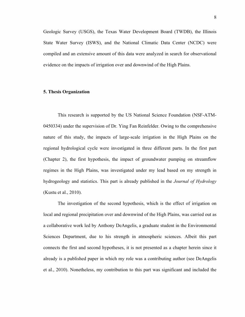
Figure 1.1. A simplified version of the terrestrial water cycle showing its reservoirs and
the complex dynamic interactions among them…………………………………. 10
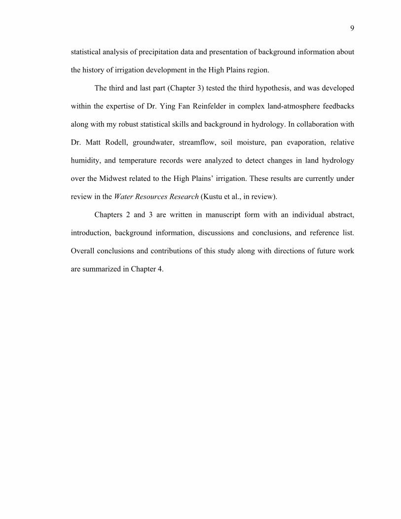
Figure 1.2. Diagram explaining the concept of streamflow depletion by pumping (Winter
et al., 1998)……………………………………………………………………….11
Figure 1.3. The change in the major perennial streams in Kansas from 1961 to 1994
(Sophocleous, 2000)……………………………………………………………...12
Figure 1.4. Water level changes in the High Plains from predevelopment to 2007
(reproduced from McGuire, 2009). The insert shows volume of groundwater
pumped for irrigation from the High Plains aquifer by state for selected years
between 1949 and 1995 (McGuire et al., 2003)…………………………………. 13
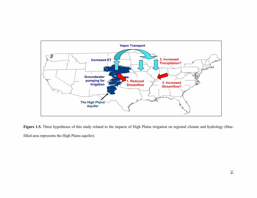
Figure 1.5. Three hypotheses of this study related to the impacts of High Plains irrigation
on regional climate and hydrology (blue-filled area represents the High Plains
aquifer)…………………………………………………………………………... 14
Figure 2.1. (a) A simplified version of the terrestrial water cycle showing its reservoirs
and the complex dynamic interactions among them (red arrows indicate fluxes
most directly affected by pumping); numbers 1-4 indicate impacts of pumping on
local river flow, regional river flow, ET, and P, and (b) objectives of this study,
showing the three components of the irrigation-induced water cycle and focus of
the report (filled area represents the High Plains aquifer)………………………..71
Figure 2.2. (a) Location and topography of High Plains regional aquifer system (from Qi
et al., 2002), (b) Average annual precipitation (blue) and Class-A pan evaporation

xi
(red) in the High Plains from 1951-1980 (from Kastner et al., 1989), and (c) water
level changes in the High Plains from predevelopment to 2007 (reproduced from
McGuire, 2009), where insert shows volume of groundwater pumped for
irrigation from the High Plains aquifer by state for selected years between 1949
and 1995 (from McGuire et al., 2003)…………………………………………... 72
Figure 2.3. Map with all the hydrologic sites examined for this study. Base map
(McGuire, 2009) shows the water-level changes in the High Plains aquifer from
pre-development to 2007………………………………………………………... 73
Figure 2.4. Locations of the streamflow, groundwater and precipitation sites used in the
step-change analysis……………………………………………………………... 74
Figure 2.5. Locations of the streamflow, groundwater and precipitation sites discussed in
the analysis of groundwater-surface water connection. (Blue and green stars
indicate the groundwater wells used in the seasonal cycle and elevation analysis,
respectively.)…………………………………………………………………….. 75
Figure 2.6. Mean seasonal cycles of streamflow vs. local precipitation, streamflow vs.
groundwater table elevation, and autocorrelation plots for the analyzed sites.
(Error bars represent one standard deviation)……..…………………………….. 76
Figure 2.7. Spatial distribution of trend analysis based on a) mean annual streamflow, b)
mean dry-season streamflow, c) number of low-days, and step change analysis
based on d) long-term streamflow, e) dry-season streamflow, f) number of low-
flow days. (&: stream gauge with decreasing trend, %: stream gauge with
increasing trend, ": stream gauge with no trend, and $: stream gauge with %
change)…………………………………………………………………………... 78
xii
Figure 2.8. Time series of mean July-August flow at the gauges that fail to show
significant trends in dry-season flow but have decreasing trends in the mean
annual flow……………………………………………………………………….80
Figure 2.9. Spatial distribution of trend analysis based on a) total annual precipitation, b)
total dry-season (mean July and August) precipitation. (&: precipitation station
with decreasing trend, and ": precipitation station with no trend)…………….…81
Figure 2.10. Results of this study (in black boxes) together with the findings from earlier
studies (in red boxes) related to the changes in streamflow variables over the High
Plains aquifer……………………………………………………………………..82
Figure 3.1. (a) Volume of groundwater pumped for irrigation from the US High Plains
aquifer for selected years, (b) the resulting water table decline (both from
McGuire et al. 2003), and (c) possible effects of High Plains irrigation on the
regional water cycle……………………………………………………………. 114
Figure 3.2. (a) Spatial pattern of July precipitation change (%) between periods of (1900-
1950) and (1950-2000) and mean July 850 mb wind fields (m/s) over 1979-2001,
obtained from North America Regional Reanalysis (for details see DeAngelis et
al. 2010), (b) time series of July precipitation (mm) averaged over 316 station
records within Region 3 (green box in b), shown as 5-year moving average and
with mean (blue) of the first and second half of the century (84 and 102 mm,
respectively, tested statistically significant in DeAngelis et al. (2010)). The green
box is the area of focus in this study…………………………………………… 115
xiii
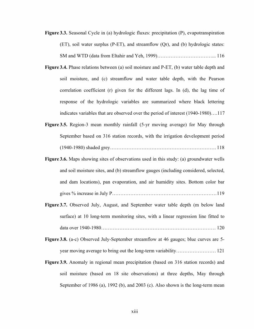
Figure 3.3. Seasonal Cycle in (a) hydrologic fluxes: precipitation (P), evapotranspiration
(ET), soil water surplus (P-ET), and streamflow (Qr), and (b) hydrologic states:
SM and WTD (data from Eltahir and Yeh, 1999)……………………………... 116
Figure 3.4. Phase relations between (a) soil moisture and P-ET, (b) water table depth and
soil moisture, and (c) streamflow and water table depth, with the Pearson
correlation coefficient (r) given for the different lags. In (d), the lag time of
response of the hydrologic variables are summarized where black lettering
indicates variables that are observed over the period of interest (1940-1980)….117
Figure 3.5. Region-3 mean monthly rainfall (5-yr moving average) for May through
September based on 316 station records, with the irrigation development period
(1940-1980) shaded grey………………………………………………………. 118
Figure 3.6. Maps showing sites of observations used in this study: (a) groundwater wells
and soil moisture sites, and (b) streamflow gauges (including considered, selected,
and dam locations), pan evaporation, and air humidity sites. Bottom color bar
gives % increase in July P……………………………………………………… 119
Figure 3.7. Observed July, August, and September water table depth (m below land
surface) at 10 long-term monitoring sites, with a linear regression line fitted to
data over 1940-1980…………………………………………………………… 120
Figure 3.8. (a-c) Observed July-September streamflow at 46 gauges; blue curves are 5-
year moving average to bring out the long-term variability…………………… 121
Figure 3.9. Anomaly in regional mean precipitation (based on 316 station records) and
soil moisture (based on 18 site observations) at three depths, May through
September of 1986 (a), 1992 (b), and 2003 (c). Also shown is the long-term mean

xiv
water table depth distribution (d) based on 34 wells in Illinois (data source: USGS
and WRAM and ICN groundwater monitoring networks, both run by ISWS (data
in Table 3.1))…………………………………………………………………… 124
Figure 3.10. July mean maximum daily temperature (C) averaged over 104 stations (a),
and July station pan evaporation (mm) at one site in IL (b) and 5 sites in IN (c, d,
e, f, g) (5-yr moving average in blue)………………………………………... 125
Figure 3.11. July surface air temperature and relative humidity (left), and vapor pressure
deficit (right) at 3 stations in Illinois and Indiana (locations shown in Fig. 3.6b),
with 5-yr moving average shown in think lines………………………………... 126
Figure 3.12. Changes in streamflow seasonal cycle at the 46 gauges (as % annual
total)……………………………………………………………………………. 127
1
Chapter 1
Introduction
1. Background
The terrestrial water cycle (TWC) forms a fundamental link between natural
ecosystems and global climate, and controls the circulation of water and energy over the
continent. Dynamic interactions at diverse spatial (local-regional) and temporal
(seasonal-decadal) scales among the TWC components such as groundwater, streamflow,
and soil moisture creates a highly complex system complicating the identification and
quantification of linkages among them (Fig. 1.1).
Human alterations, on the other hand, pose further challenges for the detection
and attribution of changes in each hydrologic component. Throughout the globe, the
natural distribution of water over the continents is continuously being modified primarily
in the form of land-use changes, flow regulations and irrigation. Understanding the
impacts of these alterations on regional hydrology and climate can greatly improve future
climate change predictions and water resources management.
Irrigation is one of the most common direct human alterations of the hydrological
cycle (e.g. Vorosmarty and Sahagian, 2000; Foley et al., 2005; Zhang et al., 2007;
Barnett et al., 2008; Milliman et al., 2008), and alone accounts for 85% of the global
water consumption (Gleick, 2003). The ways in which irrigation can alter the
hydrological cycle are manifold as numerous studies have shown the discernible effects
of irrigation water use on evapotranspiration, precipitation, streamflow, and groundwater

2
at multi-spatial scales (e.g. Chase et al., 1999; Boucher et al., 2004; Milly et al., 2005;
Douglas et al., 2006; Wen and Chen, 2006; Adegoke et al., 2007). The most recognized
effects of irrigation on regional hydrology and climate are:
1) Depletion of streamflow by groundwater pumping for irrigation:
Groundwater is the primary source of irrigation in most arid and semi-arid regions where
surface water is limited. In such regions, extensive pumping of groundwater results in
decreased groundwater storage as the natural aquifer recharge rates are very low.
Furthermore, persistent pumping for irrigation might lead to depletion of streamflow as a
result of reduced baseflow to rivers (Winter et al., 1998; Sophocleous, 2002; Douglas et
al., 2006). The adverse effect of pumping on streams is particularly stronger in areas of
close groundwater-streamflow connection where groundwater is the principal source of
streamflow. In such areas, groundwater discharges to a stream under normal conditions,
however, when a well is pumped near the stream, the natural balance is disturbed and part
of the groundwater that would have normally discharged to the stream starts to flow into
the well. As the pumping rate increases, the well captures more groundwater and finally
intercepts flow of the stream causing streamflow depletion (Fig. 1.2). A good example is
the disappearance of numerous perennial streams in the western third of Kansas between
1961 and 1994 as a result of large groundwater withdrawals for irrigation (Sophocleous,
2000) (Fig. 1.3).
2) Enhancement of evapotranspiration and precipitation: Besides depleting
groundwater storage and baseflow to rivers, irrigation dramatically increases soil
moisture during the warm season. This sudden increase in soil moisture leads to a
temporary increase in the atmospheric water vapor through enhanced evaporative flux

3
(Boucher et al., 2004; Gordon et al., 2005). Higher evapotranspiration (ET) rates and
atmospheric moisture content during warm season promotes the formation of convective
rainfall when conditions are favorable for convection. However, immediately over
irrigated fields, irrigation-induced increases in latent heat flux and cloud cover cool the
surface temperatures and inhibit the likely formation of convection (Barnston and
Schickendanz, 1984; Lobell et al., 2008). Alternatively, surface temperatures downwind
of the irrigated areas are not affected, and, with the import of additional water vapor from
the irrigated region, convective precipitation is more likely to occur. Several studies
suggested that the irrigation-induced enhanced precipitation could be observed near the
boundaries of the irrigated fields as well as over quite distant areas from the irrigated
regions (Barnston and Schickendanz, 1984; Segal et al., 1989; Moore and Rojstaczer,
2002; Pal and Eltahir, 2002; Jodar et al., 2010).
3) Effect of enhanced precipitation on variables of land hydrology: The
increase in precipitation caused by irrigation would have hydrologic consequences on
land hydrology as the seasonal variability of precipitation has a large control on the
seasonal variability of other hydrologic variables such as soil moisture, streamflow, and
groundwater. Precipitation partitioning in a given region might occur in various ways
(canopy interception, infiltration, surface runoff, ET, groundwater recharge) based on
landscape factors (e.g. topography, soil, and vegetation). The additional rainfall might
either return to the atmosphere through ET or run off to streams or infiltrate through the
soil surface. Each of these processes occurs at different time scales depending on the soil
wetness determined by earlier weather conditions (Falkenmark et al., 1999). In that sense,
soil moisture is the key to determine the amount of precipitation that will contribute to

4
ET, and to streamflow and groundwater. In water-limited regions where potential water
demand exceeds water supply, the surplus rainfall would tend to increase ET with limited
or no contribution to streams and aquifers. Alternatively, in energy-limited regions where
water supply is greater than potential water demand, precipitation is more likely to
infiltrate through the soil profile recharging the water table and, hence, increasing
baseflow to rivers (Budyko, 1974; Donohue et al., 2007; Ryu et al., 2008).
2. Research Objectives and Questions
Recent mounting evidence on the intensification (e.g. Huntington, 2006; Gerten et
al., 2008; Dery et al., 2009) and human-induced alteration of the hydrological cycle (e.g.
Costa et al., 2003; Twine et al., 2004; Foley et al., 2005; Nilsson et al., 2005; Adam and
Lettenmaier, 2008) draws more attention on the importance of identifying the correct
causes of observed changes on the hydrologic cycle. With the broader aim of
understanding the influence of human activities on the natural water cycle, this study
investigates the impacts of large-scale irrigation in the US High Plains on regional hydro-
climatic linkages and feedbacks. In this context, the main objectives of this study are; 1)
to better understand and identify large-scale human-induced changes on different
reservoirs of the hydrologic cycle at seasonal-to-decadal time scales, 2) to attribute these
changes to correct causes, and 3) to assess the impacts of these changes on regional
climate and hydrology. More specifically, the following questions are asked to address
the effects of this large-scale groundwater-based irrigation in the High Plains:
5
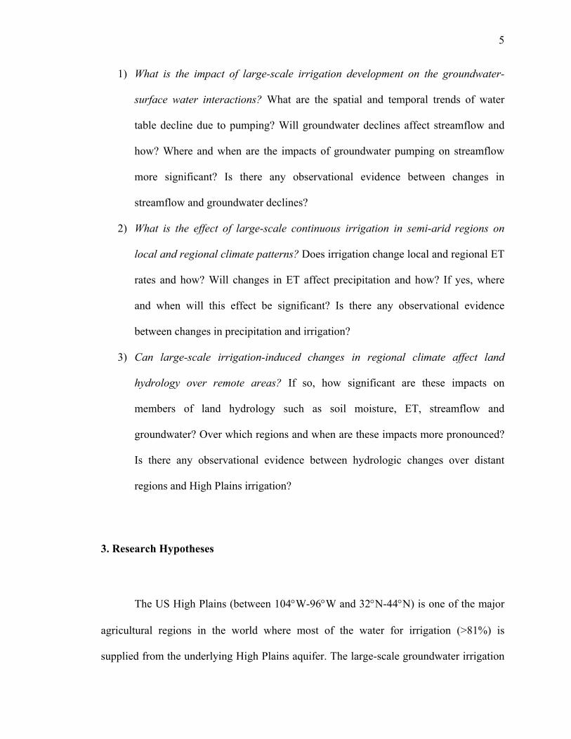
1) What is the impact of large-scale irrigation development on the groundwater-
surface water interactions? What are the spatial and temporal trends of water
table decline due to pumping? Will groundwater declines affect streamflow and
how? Where and when are the impacts of groundwater pumping on streamflow
more significant? Is there any observational evidence between changes in
streamflow and groundwater declines?
2) What is the effect of large-scale continuous irrigation in semi-arid regions on
local and regional climate patterns? Does irrigation change local and regional ET
rates and how? Will changes in ET affect precipitation and how? If yes, where
and when will this effect be significant? Is there any observational evidence
between changes in precipitation and irrigation?
3) Can large-scale irrigation-induced changes in regional climate affect land
hydrology over remote areas? If so, how significant are these impacts on
members of land hydrology such as soil moisture, ET, streamflow and
groundwater? Over which regions and when are these impacts more pronounced?
Is there any observational evidence between hydrologic changes over distant
regions and High Plains irrigation?
3. Research Hypotheses
The US High Plains (between 104W-96W and 32N-44N) is one of the major
agricultural regions in the world where most of the water for irrigation (>81%) is
supplied from the underlying High Plains aquifer. The large-scale groundwater irrigation

6
over the region resulted in a net decrease of 8.5% (330 km3) in the volume of storage of
the pre-development (pre-1950), from pre-development to 2007 (McGuire, 2009) (Fig.
1.4). In this study, it is hypothesized that the long-term irrigation development in the
High Plains has had significant hydrologic and climatic impacts not only on the region
itself but also on areas further downwind of the High Plains during the second half of the
last century (Fig. 1.5):
1) Extensive pumping of groundwater for irrigation in the High Plains depleted
streamflow, particularly in areas where streams are mainly fed by baseflow. The
substantial depletion in groundwater storage as a result of irrigational pumping caused
declines in water table levels by as much as 30 m in different parts of the High Plains
(Gutentag et al., 1984), leading to significant decreases in streamflow. There have been
numerous studies on the effect of pumping on the High Plains streamflow, but they
focused on local areas and applied different analysis methods making a regional
comparison impossible (e.g. Sophocleous 2000; 2005; Wen and Chen, 2006; Brikowski,
2008). A region-wide systematic analysis of temporal and spatial trends of streamflow
depletion was lacking despite the adverse impacts of groundwater pumping over the
region since the early 1950s.
2) Irrigation has likely enhanced warm-season precipitation downwind of the High
Plains through increased ET and vapor export. The sudden increase in soil moisture
during the irrigation season enhances ET and atmospheric water vapor in the High Plains
as most of the surplus water from irrigation evaporates rather than runs off to a stream or
recharges groundwater (Moore and Rojstaczer, 2002). It is hypothesized that the
irrigation-induced ET and water vapor over the High Plains are exported downwind by
7
the Great Plains Low Level Jet (GPLLJ) that strengthens each year during the warm
season (May-July) (Weaver et al., 2009). The GPLLJ favors convection in the Great
Plains and enters from the Gulf of Mexico propagating northward over the High Plains,
then turns eastward toward Illinois and Indiana, and finally exits at the Atlantic coast.
Therefore, it is hydrologically possible that additional moisture from the High Plains
triggered downwind warm season precipitation over Illinois and Indiana.
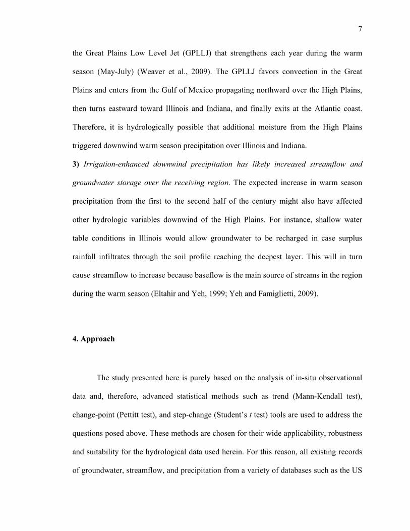
3) Irrigation-enhanced downwind precipitation has likely increased streamflow and
groundwater storage over the receiving region. The expected increase in warm season
precipitation from the first to the second half of the century might also have affected
other hydrologic variables downwind of the High Plains. For instance, shallow water
table conditions in Illinois would allow groundwater to be recharged in case surplus
rainfall infiltrates through the soil profile reaching the deepest layer. This will in turn
cause streamflow to increase because baseflow is the main source of streams in the region
during the warm season (Eltahir and Yeh, 1999; Yeh and Famiglietti, 2009).
4. Approach
The study presented here is purely based on the analysis of in-situ observational
data and, therefore, advanced statistical methods such as trend (Mann-Kendall test),
change-point (Pettitt test), and step-change (Student’s t test) tools are used to address the
questions posed above. These methods are chosen for their wide applicability, robustness
and suitability for the hydrological data used herein. For this reason, all existing records
of groundwater, streamflow, and precipitation from a variety of databases such as the US
8
Geologic Survey (USGS), the Texas Water Development Board (TWDB), the Illinois
State Water Survey (ISWS), and the National Climatic Data Center (NCDC) were
compiled and an extensive amount of this data were analyzed in search for observational
evidence on the impacts of irrigation over and downwind of the High Plains.
5. Thesis Organization
This research is supported by the US National Science Foundation (NSF-ATM-
0450334) under the supervision of Dr. Ying Fan Reinfelder. Owing to the comprehensive
nature of this study, the impacts of large-scale irrigation in the High Plains on the
regional hydrological cycle were investigated in three different parts. In the first part
(Chapter 2), the first hypothesis, the impact of groundwater pumping on streamflow
regimes in the High Plains, was investigated under my lead based on my strength in
hydrogeology and statistics. This part is already published in the Journal of Hydrology
(Kustu et al., 2010).
The investigation of the second hypothesis, which is the effect of irrigation on
local and regional precipitation over and downwind of the High Plains, was carried out as
a collaborative work led by Anthony DeAngelis, a graduate student in the Environmental
Sciences Department, due to his strength in atmospheric sciences. Albeit this part
connects the first and second hypotheses, it is not presented as a chapter herein since it
already is a published paper in which my role was a contributing author (see DeAngelis
et al., 2010). Nonetheless, my contribution to this part was significant and included the
9
statistical analysis of precipitation data and presentation of background information about
the history of irrigation development in the High Plains region.
The third and last part (Chapter 3) tested the third hypothesis, and was developed
within the expertise of Dr. Ying Fan Reinfelder in complex land-atmosphere feedbacks
along with my robust statistical skills and background in hydrology. In collaboration with
Dr. Matt Rodell, groundwater, streamflow, soil moisture, pan evaporation, relative
humidity, and temperature records were analyzed to detect changes in land hydrology
over the Midwest related to the High Plains’ irrigation. These results are currently under
review in the Water Resources Research (Kustu et al., in review).
Chapters 2 and 3 are written in manuscript form with an individual abstract,
introduction, background information, discussions and conclusions, and reference list.
Overall conclusions and contributions of this study along with directions of future work
are summarized in Chapter 4.
10
Figure 1.1. A simplified version of the terrestrial water cycle showing its reservoirs and
the complex dynamic interactions among them.
Ocean
Continental Atmosphere
Groundwater
Rivers, Lakes, Wetlands
Soil-Vegetation
Human Activities
Subsurface
Land Surface
Terrestrial Water Cycle
11
Figure 1.2. Diagram explaining the concept of streamflow depletion by pumping (Winter
et al., 1998).

12
Figure 1.3. The change in the major perennial streams in Kansas from 1961 to 1994
(Sophocleous, 2000).

13
Figure 1.4. Water level changes in the High Plains from predevelopment (i.e. before
1950s) to 2007 (reproduced from McGuire, 2009). The insert shows volume of
groundwater pumped for irrigation from the High Plains aquifer by state for selected
years between 1949 and 1995 (McGuire et al., 2003).
104 102106 108 100 98 96
40
37
43
34
14
Figure 1.5. Three hypotheses of this study related to the impacts of High Plains irrigation on regional climate and hydrology (blue-
filled area represents the High Plains aquifer).
1. Reduced Streamflow 3. Increased
Streamflow?
Groundwater pumping for
Irrigation
2. Increased Precipitation?
The High Plains Aquifer
Vapor Transport
Increased ET
15
Chapter 2
Large-scale Water Cycle Perturbation due to Irrigation Pumping in the US High
Plains: A Synthesis of Observed Streamflow Changes
Abstract
The influence of long-term, large-scale irrigational pumping on spatial and
seasonal patterns of streamflow regimes in the High Plains aquifer is explored using
extensive observational data to elucidate the effects of regional-scale human alterations
on the hydrological cycle. Streamflow, groundwater and precipitation time series
spanning all or part of the period of intensive irrigation development (1940-1980) in the
region were analyzed for trend and step changes using the non-parametric Mann-Kendall
test and the parametric Student’s t-test, respectively. Based on several indicators to
evaluate the degree of streamflow-groundwater connection over the High Plains aquifer,
a systematic decrease in the hydraulic connection between groundwater and streamflow
from the Northern High Plains to Southern High Plains was found. Trends and step
changes are consistent with this regional pattern. Trends in decreasing annual and dry-
season (mean July-August) streamflow and in increasing number of low-flow days are
prevalent in the Northern High Plains. Number of significant trends gradually decreases
towards the south. Additionally, field significance of trends was assessed by the Regional
Kendall’s S test over the period of most intensive irrigation development (1940-1980).
The step change results imply that the observed decreases in streamflow are likely

16
attributable to the significant declines in groundwater levels and unlikely related to
changes in precipitation because the majority of precipitation data over the region did not
reveal any significant changes. Thus, it is very likely that extensive irrigational pumping
have caused streamflow depletion, more severely, in the Northern High Plains, and to a
lesser extent in the Southern High Plains over the period of study.
17
1. Introduction
The terrestrial water cycle forms a vital link between natural ecosystems and the
global climate through complex interactions among its components. Identification and
quantification of linkages between the components of the water cycle is further
complicated because each component is linked to every other, either in direct or indirect
ways, via dynamic flux exchange across a wide range of spatial and temporal scales (Fig.
2.1a). Thus, any change in one of the storages will have a subsequent effect on the other
parts of the water cycle and on the natural hydrological fluxes. However, our knowledge
of the potential impacts of these changes on the other components of the water cycle,
along with their spatial scales or regional significance, is still very limited yet crucial for
future climate variability prediction and water resources management.
Recent studies showed that, besides natural processes, human activities distinctly
alter the hydrological cycle by disturbing the natural circulation of water over the
continent (Costa et al., 2003; Foley et al., 2005; Nilsson et al., 2005; Huntington, 2006;
Zhang et al., 2007; Adam and Lettenmaier, 2008; Barnett et al., 2008; Sahoo and Smith,
2009). One major cause of these disturbances is irrigation (Alpert and Mandel, 1986;
Vorosmarty and Sahagian, 2000; Milly et al., 2005; Haddeland et al., 2006b; 2007;
Milliman et al., 2008; Gerten et al., 2008; Rost et al, 2008b; Wisser et al., 2009), which
accounts for nearly 85% of the global water consumption (Gleick, 2003). In fact, the
primary use of water worldwide is to irrigate the agricultural areas, which cover 40% of
the land surface (Asner et al., 2004). As the demand for food increases along with the
growing population, irrigated areas continue to expand with an actual expansion of 70%

18
in the last 40 years (Gleick, 2003), and consequently, surface water and groundwater
resources are being substantially exploited to comply with the corresponding increase in
water demand. Lately, the global use of groundwater has surpassed surface water use as
the primary source of irrigation (Healy et al., 2007; Giordano and Villholt, 2007), such
that the total groundwater withdrawals for irrigation have increased from 23% of total
withdrawals for irrigation in 1950 to 42% of that in 2000 for the conterminous USA
(Hutson et al., 2004). Most of the water extracted from aquifers for irrigation is lost into
the atmosphere by evapotranspiration (ET) after it is applied to the land surface, while the
rest either runs off to a stream or infiltrates through the soil zone becoming groundwater
again. Due to the interactions among the reservoirs of the hydrological cycle, this
disturbance will have subsequent effects on local and regional river flow (fluxes 1 and 2
in Fig. 2.1a), on ET (flux 3), and consequently on precipitation (flux 4). Accordingly,
extensive pumping of groundwater leads to depleted subsurface storages, especially in
arid and semi-arid regions where the natural aquifer recharge rates are very low. Over the
last century, groundwater levels across the United States declined substantially, generally
during the dry-season and in semi-arid regions, as a result of increased groundwater
usage for irrigation (Bartolino and Cunningham, 2003). Furthermore, groundwater
mining is a growing problem throughout the world which adversely affects major aquifer
systems as well as local areas (Konikow and Kendy, 2005). One well-known case is the
High Plains aquifer system of the US Great Plains, where large-scale irrigational
pumping induced a depletion of more than 330 km3 in the stored volume of water, a net
decrease of 8.5% of the pre-development (i.e. before irrigation) water in storage, from
pre-development (about 1950) to 2007 (McGuire, 2009).
19
One direct effect of groundwater irrigation is the significant reduction of surface
water availability, also known as “streamflow depletion”, due to decreased groundwater
discharge to streams and wetlands caused by excessive and prolonged pumping (Winter
et al., 1998; Sophocleous, 2002; Kollet and Zlotnik, 2003). The impact can be large
especially in areas where groundwater and surface water systems are closely-connected,
since groundwater is the principal source of streamflow in such places. For example,
many perennial streams in western Kansas running across the High Plains aquifer in 1961
became shorter or disconnected, or disappeared by 1994 as a result of large groundwater
withdrawals (Sophocleous, 2000). Additionally, the flow of streams in some parts of
Kansas, Oklahoma and New Mexico has decreased to half of the initial recorded flow
over time (Brikowski, 2008). A trend detection study by Wahl and Wahl (1988)
identified decreasing trends in the annual mean flow, annual baseflow, and annual peak
discharge of the Beaver River in the Oklahoma Panhandle from 1938 to 1986 while
precipitation records showed no trend for the same period. Thus, they concluded that
increased groundwater pumping from the underlying High Plains aquifer was the main
mechanism generating the observed decreases in streamflow. Szilagyi (1999) examined
the changes in the annual mean flow of Republican River basin where significant
streamflow depletion is observed since the late 1940s. Analyzing eight US Geological
Survey (USGS) gauging stations, he verified significant decreasing trends in the whole
river basin that cannot be explained by precipitation variability. Subsequently, his
modeling study (Szilagyi, 2001) showed that the observed streamflow depletion in the
same river basin has resulted from human-induced changes such as irrigation, land cover
changes and reservoir construction. Similarly, Burt et al. (2002) applied a multiple

20
regression model to annual streamflow data from a single gauging station in the
Republican River basin to evaluate the effect of groundwater irrigation on streamflow
during the period 1936-1998 and found a strong inverse relationship between annual
streamflow and the number of irrigation wells, in addition to a 75% decline in the mean
annual flow over the same period. In a more comprehensive study, Wen and Chen (2006)
searched for trends in streamflow using data from 110 gauging stations in eight major
river basins throughout Nebraska during 1948-2003 and detected decreasing trends at the
majority of gauges in the Republican River basin but only at a few in the eastern part.
Without any significant changes in precipitation and temperature for the same period,
their study concluded that groundwater withdrawal for irrigation was the primary factor
leading to depletion of streamflow in Nebraska. Also, Buddemeier et al. (2003) reported
that after the onset of extensive groundwater pumping, portions of major rivers crossing
the High Plains aquifer experienced decreases in annual flow during the last few decades
with the Arkansas River exhibiting the greatest flow depletion among the others.
Besides depleting the groundwater storage and reducing the baseflow to rivers,
irrigation dramatically increases soil moisture during the warm season which may
instigate indirect effects on the key components of regional climate including increases in
ET, cooling of surface temperatures and enhancement of precipitation (the fourth link in
Fig. 2.1a) (Eltahir and Bras, 1996; Eltahir, 1998; Vorosmarty and Sahagian, 2000; Pielke,
2001; Kanamitsu and Mo, 2003; Betts, 2004; Haddeland et al., 2006a). Several modeling
studies showed that an increase in soil moisture induces higher ET and atmospheric
moisture content which further contributes to the formation of local convective storms via
enhanced moisture recycling over or downwind of the irrigated (or wetted soil) regions

21
(e.g., Segal et al., 1989; Small, 2001; Pal and Eltahir, 2002; Koster et al., 2004;
Dominguez et al., 2009). One study investigated the effect of land use changes on the
regional climate of the irrigation-dominated northern Colorado plains (Chase et al.,
1999). Their model results demonstrated that the magnitude of forcing induced by
irrigational practices were strong enough to affect the regional temperature, cloud cover,
precipitation and surface hydrology. Other regional studies showed significant
differences in the heat and moisture fluxes between the irrigated (wet) and non-irrigated
(dry) areas over India (Douglas et al., 2006), and Nebraska (Adegoke et al., 2007).
Despite the intricacy of this mechanism, few observational studies detected a signal of
irrigation-precipitation link over the High Plains aquifer. One study identified an
irrigation-related increase in June precipitation during 1930-1970 over and near the
heavily-irrigated regions in the Texas panhandle when synoptic conditions allowed low-
level convergence and uplift (Barnston and Schickendanz, 1984). Another one observed
an additional summer rainfall of 6-18% about 90 km downwind of the Texas panhandle
during 1996 and 1997 (Moore and Rojstaczer, 2002). A third study by Adegoke et al.
(2003) found cooler surface temperatures in summer within the densely-irrigated areas in
Nebraska verified by both simulations and data analysis.
All of these earlier studies underline that irrigation significantly influences the
climate and hydrology patterns not only at local scales but also at regional scales (Fig.
2.1b). Therefore, in this study, we aim to develop a comprehensive analysis of the
regional impacts of irrigational pumping on the hydrological cycle to investigate whether
an anthropogenic regional water cycle is embedded into the natural and continental-scale
water cycle. Our research will be reported in a series of three papers. In this first paper,

22
we investigate the direct effect of groundwater irrigation: streamflow depletion. In a
second study, we analyze observed precipitation over the central US searching for signals
of irrigation-enhanced precipitation downwind of the High Plains (DeAngelis et al.,
2010). In a third report, we examine the observed groundwater and streamflow downwind
of the High Plains where enhanced precipitation has been observed (Kustu et al., under
review). We emphasize that all three studies rely on long-term observations in
groundwater, streamflow and precipitation, and that our attention is on the regional-scale
hydrologic and climatic linkages and feedbacks.
The focus of this paper is to determine the long-term, large-scale irrigational
pumping effects on the spatial and seasonal patterns of streamflow regimes over the High
Plains aquifer. There have been numerous observational and theoretical studies that
investigated the groundwater-surface water interactions, however their focus are the
changes in small watershed scales (e.g., Hewlett and Hibbert, 1963; Dunne and Black,
1970a,b; Tanaka et al., 1988; De Vries, 1994, 1995; Eltahir and Yeh, 1999; Marani et al.,
2001; Nyholm et al., 2003; Chen and Chen, 2004; Chen et al., 2008; Zume and Tarhule,
2008). Likewise, the aforementioned studies on streamflow trends in the High Plains
aquifer concentrated at one to a few river basins, used different streamflow gauges and
analysis methods, over different time periods, and, thus, lack a region-wide,
methodologically consistent picture of where and when streamflow depletion is
significant. No systematic effort yet has been made to understand the regional
significance of groundwater pumping on streamflow despite the large-scale groundwater
depletion observed in the aquifer since the 1930s. Hence, this paper will tie the scattered
evidence together and establish the regional pattern of streamflow depletion, based on
23
streamflow observations in conjunction with precipitation and water table data using all
available records in the USGS archive.
Moreover, detection of abrupt (step) and gradual changes in hydrologic variables
and comprehension of their likely causes are critical for long-term water management and
assessment of future changes. The attribution of these changes to correct causes is more
crucial than ever under the presence of long-term, CO2-induced climate change trends.
Most trend analysis studies attribute the observed changes in streamflow to the variations
in climate (e.g. Lins, 1985; Dery and Wood, 2005; Miller and Piechota, 2008). Here, we
hypothesize that large-scale human activities, such as the irrigation development in the
High Plains region, may induce drastic, regional-scale changes in the hydrological cycle
in a similar magnitude as caused by climate variability.
The specific objectives of this study are: 1) to examine the climatic, geologic, and
hydrologic variabilities across the High Plains; patterns emerging from this analysis will
shed light on where, along the climatic and hydrologic gradient, streamflow is most likely
affected by groundwater pumping, 2) to examine the degree of hydraulic connection
between the groundwater and streamflow across the climatic-hydrologic gradient;
patterns emerging from this analysis will further pinpoint regions/settings where
groundwater pumping is most likely to affect streamflow, 3) to quantify the streamflow
depletion annually and seasonally over selected regions along the climatic-hydrologic
gradient, using trend and step-change analysis tools, 4) to assess the field significance of
detected trends, and 5) to attribute the observed streamflow depletion to likely causes,
i.e., changes in rainfall or in groundwater storage. The results of this study will improve

24
our understanding and quantification of the impact of human modifications to the water
cycle at regional scales during the second half of the last century.
The following sections first provide the background information on the study
area, followed by the description of data sources and an outline of the methodology.
Then, we discuss the observed changes in streamflow across the High Plains region for
the period of intensive irrigational development using several indicators. We conclude
with a geographic synthesis of regional variations in streamflow depletion caused by
irrigational groundwater pumping.
2. The High Plains Aquifer System
The High Plains aquifer, a subregion of the Great Plains, is the largest regional
aquifer system in the US, and extends under parts of eight states from southern South
Dakota to northwestern Texas with a surface area of 450,000 km2 (Fig. 2.2a). Flat to
gently-sloping vast plains formed by stream-deposited sediments transported eastward
from the Rocky Mountains characterize the region (Dennehy, 2000). The aquifer consists
of several hydraulically-connected geologic units of Tertiary or Quaternary age. The
Brule Formation, the Arikaree Group and the Ogallala Formation constitute the upper
Tertiary rocks. The Oligocene-aged Brule Formation, a low-permeable massive siltstone
with layers of sandstone and volcanic ash, underlies parts of Nebraska, Colorado and
Wyoming and is considered as part of the aquifer only in areas where its permeability is
increased by secondary porosity. Overlying the Brule Formation is the Miocene- to
Oligocene-aged Arikaree Group which is composed of massive fine-grained sandstone
25
with local beds of volcanic ash, silt and clay underlying large parts of Nebraska, South
Dakota and Wyoming. Over the Arikaree Group lies the Miocene-Pliocene Ogallala
Formation of unconsolidated clay, silt, sand and gravel. The Ogallala Formation is the
principal geologic unit of the aquifer covering 77% of the system’s area. Unconsolidated
alluvial deposits of Quaternary age overlie the Ogallala Formation on the east and
constitute part of the aquifer in areas where they are in hydraulic connection with the
Tertiary deposits. Most of the gravel, sand, silt and clay in the alluvial deposits are
reworked material derived from the Ogallala Formation in the form of sand dunes,
windblown loess and valley-fill deposits along the stream channels (Gutentag et al., 1984;
Weeks et al., 1988). In general, the thickness of the aquifer decreases from north to south
and from central to east. The High Plains aquifer is generally underlain by Permian- to
Tertiary-aged evaporites such as anhydrite, gypsum, halite, limestone and dolomite.
The High Plains region has a typical mid-latitude dry continental climate with a
high rate of evaporation, limited precipitation and abundant sunshine changing from arid
to semi-arid from the Texas panhandle to western Kansas, and to sub-humid in some
parts of central Kansas and eastern Nebraska (Gutentag et al., 1984). The region is
characterized by natural climate gradients from east to west and north to south. Located
at the center of a transition zone, a wetter to drier precipitation gradient from east to west,
and a colder to hotter temperature gradient from north to south prevail across the region
(Fig. 2.2b). These precipitation (east-west) and temperature (north-south) gradients
produce a distinctive climate condition that varies substantially from hourly to decadal
time scales. The average annual precipitation throughout the region is 500 mm with a
range of 300 mm (Rodell and Famiglietti, 2002). Most of the precipitation falls as rain
26
during the growing season, from April to September, however large variations in rainfall
are observed both spatially and temporally due to the common thunderstorms and
extreme weather events (Weeks et al., 1988). As a result of limited precipitation,
naturally-occurring fertile soils with grassland vegetation cover the region (Kromm and
White, 1992). The evapotranspiration rates are high, because of persistent winds and high
summer temperatures, and annually average from 1500 mm in the north to 2700 mm in
the south (Weeks et al., 1988) (2.2b).
The High Plains is an unconfined blanket sand-and-gravel type aquifer with a
general groundwater direction of west to east at a rate of 0.30 m/day. The water table
reaches the surface near the rivers that are hydraulically-connected to the aquifer such as
the Platte and the Arkansas Rivers. The saturated thickness of the aquifer varies from
zero in the depositional areas of unconsolidated alluvial deposits to 300 m in north-
central Nebraska, with an average of 60 m (Weeks et al., 1988). In 1980, the depth to
water table was less than 30 m in about half of the aquifer, less than 60 m under most of
Nebraska and Kansas, and between 60 and 90 m in parts of western and southwestern
Nebraska and southwestern Kansas. In local areas of prolonged irrigational pumping, the
water table could be found at 120 m or more below the ground (Miller and Appel, 1997).
The aquifer is recharged mainly by precipitation and locally by seepage from streams.
High evapotranspiration rates lower the aquifer recharge rates to less than 13 mm/yr in
most parts, ranging from 0.6 mm/yr in Texas to 150 mm/yr in south-central Kansas,
except in areas such as Nebraska Sandhills, where rainfall infiltrates quickly through the
highly permeable sand to replenish the groundwater system (Gutentag et al., 1984).
Groundwater naturally discharges to streams and springs and directly to the atmosphere

27
by evapotranspiration in areas where the water table is near the surface. However, most
of the discharge from the High Plains aquifer occurs by pumping for irrigational use,
which results in an imbalance between the discharge and the natural recharge, changing
the volume of storage (Gutentag et al., 1984). The total volume of drainable water in
storage was estimated to be about 4010 km3 in 1980, 65% of which is in Nebraska where
the recharge rate is the greatest (Gutentag et al., 1984).
Due to the ideal topography and productive soils, High Plains is one of the major
agricultural regions in the world, consisting of approximately 20% of the irrigated land in
the US, with the aquifer supplying nearly 30% of the groundwater used for irrigation
across the United States (Luckey et al., 1986; Sophocleous, 2005). In the region, water
for irrigation is principally supplied from the aquifer (81% in 1995); however surface
water is also used for irrigational use to a limited extent (19% in 1995), especially the
Platte River in Nebraska, which supplies nearly all the surface water for irrigation (85%)
(Dennehy, 2000). In the south, use of groundwater increases (~92%) (Dennehy, 2000)
due to the scarcity of surface water resources (Buchanan et al., 2009). The development
of groundwater irrigation started in the region in the 1930s in response to a drought and
expanded rapidly from South to North by the 1960s with the invention of center-pivot
irrigation systems (Miller and Appel, 1997). The groundwater irrigation developed first
in New Mexico and Texas in 1930s, later in Oklahoma and Kansas in 1940s, and finally
in Colorado, Nebraska and Wyoming during the 1950s and 1960s (Luckey et al., 1981).
From 1940 to 1980, the total irrigated area in the region had increased from 8500 km2 to
about 56,000 km2, which was irrigated with 22 km3 of water by tapping approximately
170,000 wells that had been completed in the aquifer by 1980 (Weeks et al., 1988). This

28
resulted in a depletion of 5% (~205 km3) of the pre-development volume of stored water
from the aquifer; 70% of which was in Texas and 16% in Kansas (Gutentag et al., 1984).
As the groundwater withdrawals escalated from 5 km3 to 23 km3 from 1949 to 1974 (see
insert in Fig. 2.2c), declines in water levels in the aquifer as much as 30 m were common
in parts of Texas, Oklahoma and southwestern Kansas by 1980 (Gutentag et al., 1984).
After 1980, the average rate of decline in water levels has decreased across the aquifer
despite the continuous increase in the total irrigated area attributable, in large part, to the
above-normal precipitation rates over the region between 1980 and 1994, and, in some
part, to new pumping regulations and technologies in irrigation (Dugan and Sharpe,
1995). Water-level changes in the aquifer from pre-development to 2009 are shown in
Figure 2.2c.
3. Data and Methods
3.1 Data Sources
Stream gauge records in the High Plains were acquired from the USGS National
Water Information System (NWIS) database (USGS, 2009;
http://nwis.waterdata.usgs.gov/nwis/sw). The entire record, except for some gauges in
Texas, is in the form of daily measurements starting from the early 1930s to the present.
However, the record period of each stream gauge differs greatly such that some records
extend back to the early 1900s while some others start in the late 1970s or even in 1980s.
Most stations, especially the ones in Kansas and Texas, have interrupted records, but still
no filling-in the data gaps is performed. Hence, the influence of limited data availability

29
is noted in the evaluation of the results. Major dams and reservoirs throughout the High
Plains are listed in the National Inventory of Dams by the US Corps of Engineers
(USACE) (National Atlas, 2009; http://nationalatlas.gov/mld/dams00x.html) and their
effects are considered in the analysis. Groundwater data come from two sources: the first
one is the USGS NWIS database (http://waterdata.usgs.gov/nwis/gw), which supplied the
majority of the data, and the second is the Texas Water Development Board database
(TWDB, 2009; http://www.twdb.state.tx.us/publications/reports/GroundWaterReports/
GWDatabaseReports/GWdatabaserpt.htm), which is used to supplement the sparse USGS
observations in Texas. Table 2.1 lists the total number of streamflow gauges (431) and
groundwater monitoring wells (1040) explored for this study in the states of the High
Plains aquifer. Out of 431 stream gauging stations, 64 gauges were selected for the trend
analysis in this study (Table 2.2). These gauges are located in or downstream of the areas
where significant water table decline (>7 m) has been observed (yellow, orange, and red
patches in Fig. 2.2c) and they have long and continuous data covering at least part of the
period of intensive irrigation development (1940-1980). The record period of gauging
stations varied from a minimum of 12 years to a maximum of 86 years. Of the 64, nine
stream gauges that are located within each area of significant water table decline and
have continuous daily measurements extending back to the 1940s were used in the step-
change analysis. A total of 17 groundwater wells were used in this study, which were
selected based on the highest number of measurements for the seasonal cycle analysis,
the closest location to the stream gauges for the elevation analysis, and the longest period
of record for the step-change analysis, all discussed in detail later. In addition to the
streamflow and groundwater data, monthly precipitation totals at nine stations in the

30
vicinity of the associated streamflow gauges was acquired from the Global Historical
Climate Network (GHCN, 2009) station dataset (Vose et al., 1992) using the NOAA
NCDC GHCN beta version 2, accessible via IRI/LDEO Climate Data Library
(http://iridl.ldeo.columbia.edu/SOURCES/.NOAA/.NCDC/.GHCN/.v2beta/). Tables 2.3
and 2.4 list detailed information about the precipitation stations and groundwater wells
used in this study, respectively. Figure 2.3 shows the spatial distribution of all streamflow
gauges, groundwater wells and precipitation stations considered for this study together
with the dams in the High Plains.
3.2. Methodology
In this study, trend and step changes in time series of several hydrologic variables
were analyzed in an effort to evaluate the impact of groundwater pumping on streamflow
regimes in the High Plains region. While trend analysis has been applied widely in
environmental sciences (e.g., Hirsch and Slack, 1984; Lins, 1985; Lettenmaier et al.,
1994; Lins and Slack, 1999; Douglas et al., 2000; Zhang et al., 2001; Pilon and Yue,
2002), few studies searched for an abrupt step change in water resources data (McCabe
and Wolock, 2002; Costa et al., 2003; Miller and Piechota, 2008; Kalra et al., 2008).
Identification of a step change is equally important because it gives an estimate to
quantify the amount of change caused by a certain factor over two different periods of
time, especially when relatively sudden, step-like changes are expected.
In hydrologic trend studies, non-parametric methods that do not rely on any
assumption about the underlying distribution of the data are preferred to the traditional
31
parametric methods which assume that the data are drawn from a given probability
distribution. This is because hydrological data are often strongly non-normal, typically
show autocorrelation and/or spatial correlation, and usually consist of seasonal variations
and, hence, do not usually conform to the assumptions (e.g., normality, independence,
and linearity) of the standard parametric methods (e.g., t-test, analysis of variance, linear
regression) (Helsel and Hirsch, 1992). Additionally, non-parametric methods are found to
be more robust than their parametric equivalents, along with the advantages of having
simpler and wider applicability, and being less sensitive to outliers in the data
(Kundzewicz and Robson, 2004). While we acknowledge the more sophisticated
statistical tools used in the detection of regional trends in hydrology (e.g. Katz et al.,
2002; Renard et al., 2006), in this study, we will use the non-parametric Mann-Kendall
test (Mann, 1945; Kendall, 1975) for its robustness, simplicity, and insensitivity to
missing data.
3.1.1. Mann-Kendall Test
The Mann-Kendall test is a rank-based approach that tests for randomness against
trends in time-series data and has been widely used in hydrologic and climatic trend
studies (e.g., Lins and Slack, 1999; Yue et al., 2003; Burn et al., 2004; Kahya and
Kalayci, 2004; Dery and Wood, 2005; Aziz and Burn, 2006). The null hypothesis H0
states that a sample of data (x1, x2,…, xn) consists of n independent and identically
distributed random variables, whereas the alternative hypothesis H1 is that a monotonic
trend exists in the data. The test first ranks the entire observations according to time, and
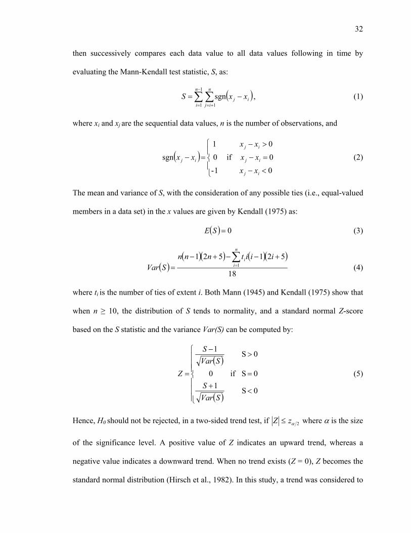
32
then successively compares each data value to all data values following in time by
evaluating the Mann-Kendall test statistic, S, as:
1
1 1
sgnn
i
n
ijij xxS , (1)
where xi and xj are the sequential data values, n is the number of observations, and
0 1-
0 if 0
0 1
sgn
ij
ij
ij
ij
xx
xx
xx
xx (2)
The mean and variance of S, with the consideration of any possible ties (i.e., equal-valued
members in a data set) in the x values are given by Kendall (1975) as:
0SE (3)
18
5215211
n
ii iiitnnn
SVar (4)
where ti is the number of ties of extent i. Both Mann (1945) and Kendall (1975) show that
when n ≥ 10, the distribution of S tends to normality, and a standard normal Z-score
based on the S statistic and the variance Var(S) can be computed by:
0S 1
0S if 0
0S 1
SVar
S
SVar
S
Z (5)
Hence, H0 should not be rejected, in a two-sided trend test, if 2zZ where is the size
of the significance level. A positive value of Z indicates an upward trend, whereas a
negative value indicates a downward trend. When no trend exists (Z = 0), Z becomes the
standard normal distribution (Hirsch et al., 1982). In this study, a trend was considered to

33
be in evidence when the null hypothesis is rejected at a significance level of 5% (i.e. =
0.05) for a two-tailed test. A robust estimate for the trend magnitude, determined by
Hirsch et al. (1982), is given by the slope estimator ():
ij
xxMedian ij for all j>i (6)
where xi and xj are the data values at times i and j, respectively.
Concerns emerge for the application of the Mann-Kendall test under the presence
of positive serial correlation and/or cross-correlation in the data series. It is recognized
that both can increase the probability of detecting a trend when, in fact, there is no trend,
leading to the incorrect rejection of the null hypothesis of no trend while it is true
(Lettenmaier et al., 1994; von Storch and Navarra, 1995; Yue et al., 2002). Several
approaches have been proposed to eliminate the possibility of overestimation caused by
serial correlation in the hydrologic series. The most common approach is to “pre-whiten”
the series prior to applying the trend test (von Storch and Navarra, 1995). However,
opinion varies on the impacts of pre-whitening, and other approaches were suggested
(Yue et al., 2002, 2003; Bayazit and Onoz, 2007; Hamed, 2009). Here, the effect of serial
correlation is not considered, because we apply the trend test to annual data values which
are approximately independent and, hence, do not exhibit serial correlation.
On the other hand, the effect of spatial correlation has generally been disregarded
in most hydrologic trend studies, despite the fact that neglecting the presence of spatial
dependence among sites in a specific region might lead to misleading results (Douglas et
al., 2000; Yue and Wang, 2002; Renard et al., 2008; Khaliq et al., 2009). In this study, we

34
use the Regional Kendall’s S test developed by Douglas et al. (2000) to account for the
effect of spatial correlation in streamflow data.
3.1.2. Regional Kendall’s S test
Douglas et al. (2000) developed a new test statistic named as regional average
Kendall’s S ( mS ) to evaluate the field (regional) significance of trends rather than local
(at individual sites) significance. The regional Kendall’s S is calculated as the average of
S values for all individual sites by:
m
kkm S
mS
1
1 (7)
where Sk is Kendall’s S for the kth station in a region with m stations. Under the presence
of cross correlation, the variance of mS becomes
xxm mm
SVar 11
2
(8)
where xx is the average cross-correlation coefficient of the region,
1
21
1 1,
mm
m
k
km
llkk
xx
(9)
and lkk , is the cross-correlation coefficient between stations k and k+l ,
),(
2
,lkk
lkk SSCov
(10)
Finally, the test statistic mZ for correlated data series is evaluated as:
mmm SVarSZ / (11)

35
In this study, the field significance of trends in mean annual flow, mean dry-
season flow, and number of low-flow days are evaluated at the 5% significance level (i.e.,
= 0.05) for a two-tailed test.
3.1.3. Student’s t-test
The student’s t-test, used here to detect step-changes, is a classical parametric test
used to check if the means of two independent groups are statistically different. The null
hypothesis H0 is that the means of two groups are equal; whereas the alternative
hypothesis H1 is that the means are not equal. Basically, the test assumes that the data are
normally-distributed and the time of change is known (Kundzewicz and Robson, 2000).
For two groups with unequal variances the test statistic, t, is given by:
2
22
1
21
21
n
s
n
s
xxt
(12)
where x1, s1 and n1 are the mean, the sample standard deviation, and the number of
observations of the first group, respectively, and x2, s2 and n2 are the mean, the sample
standard deviation, and the number of observations of the second group, respectively
(Helsel and Hirsch, 1992). Also, the degrees of freedom, df, is calculated approximately
as (Helsel and Hirsch, 1992):
11 2
2
222
1
2
121
2
2221
21
n
ns
n
ns
nsnsdf (13)

36
All step-change results herein are evaluated at the 5% significance level (i.e.,
=0.05) for a two-tailed test. For sample sizes larger than 40 (n > 40), the z-test statistic is
calculated instead of a t-test statistic. For the purpose of step-change analysis, streamflow
time series are divided into two parts: a 10-year long period (1941-1950, pre-irrigation)
and a 20-year long period (1961-1980, post-irrigation). The first period is only 10 years
due to the lack of groundwater records before 1941, and the need to select common
periods across all stations for spatial comparison. Even so, only nine wells with sufficient
data could be found near the stream gauges for this analysis. The interval 1951-1960 is
the transition period and was discarded to allow for a less ambiguous step-change
detection. To attribute the observed changes in streamflow to either changes in
precipitation or in groundwater, monthly precipitation and daily water table data nearby
were also analyzed by the same approach. The streamflow, groundwater and precipitation
sites used in the step-change analysis are shown in Figure 2.4.
4. Results and Discussion
4.1. Regional Patterns of Groundwater-Surface Water Connection
The greatest impact of irrigational pumping is likely to be observed in areas
where streams are in hydraulic connection with the groundwater system since, in such
areas, streams receive a significant portion of their inflow from the groundwater. The
amount of groundwater contribution to streamflow varies depending on the
hydrogeologic and climatic conditions. The key is whether a stream is predominantly

37
surface runoff- or groundwater-fed. In arid regions with isolated summer thunder storms,
surface runoff is the primary source for stream flow, and the water table is below the
stream bed. In humid climates with frequent rain, infiltration is favored, which recharges
the groundwater and enter the streams as baseflow long after the rain events. Controlling
this partition (surface runoff vs. infiltration) is also terrain slope and soil permeability.
The hydro-climatic conditions across the High Plains exhibit a north-south increase in
temperature, a west-east increase in annual precipitation, a north-south and a central-east
decrease in aquifer thickness, and a heterogeneous and anisotropic distribution of
horizontal hydraulic conductivity. Thus, it is likely that there are significant spatial
variations in the degree of hydraulic connectivity between groundwater and streamflow.
There are several indicators that can tell us whether a stream is primarily fed by surface
runoff (locally or upstream) or by groundwater inflow, based on simple analyses of
precipitation, water table and streamflow. Streamflow stations used here were selected
out of 64 stations listed in Table 2.2 based on the following criteria: 1) all have
continuous daily measurements, 2) all record the flows from approximately the same size
of drainage area (±15%), and 3) none are affected by dams. The water table data belong
to the well with the most number of observations closest to the associated stream gauges.
The locations of the streamflow, groundwater and precipitation sites used in the analysis
of groundwater-surface water connection are shown in Figure 2.5.
First, the phase relationship between the seasonal cycle of streamflow and that of
the local rainfall and water table is examined. Local rainfall is a good surrogate for
surface runoff and should have similar seasonal patterns. If the peak of streamflow leads
the peak of rainfall, then the latter is not likely the main source. The phase relationships
38
of the seasonal cycle between local rainfall and streamflow for selected sites are shown in
Figure 2.6 (first column). From north to south (a-f), a pattern seems to emerge; in the
north (Nebraska and Colorado), streamflow peaks before local rainfall, a clear indication
that the latter is not the main source for streamflow, and there is another mechanism
causing discharge to increase in early spring. The peak of rainfall in late spring/early
summer is typical since much of precipitation occurs in the form of local thunderstorms
during the growing season (April-September) (Weeks et al., 1988). However, the
streamflow peak occurs much earlier, in the spring, suggesting that the flow regime is
controlled by the groundwater which is sourced in the Rockies to the west and responds
strongly to seasonal snowmelt (Gutentag et al., 1984). Large-scale west-east groundwater
flow in the highly permeable Ogallala formation of the aquifer is well documented
(Gutentag et al., 1984; Weeks et al., 1988; Miller and Appel, 1997). This suggests that, in
the northern part of the High Plains, groundwater is the primary source of streamflow,
and, therefore, changes in groundwater storage will affect rivers more significantly. This
is not surprising since Nebraska is recognized as one of the regions with the highest
groundwater contribution to streams (up to 90%) across the USA, due to the highly-
permeable sandy soils underlying the Nebraska Sand Hills that provide important
recharge areas for the aquifer (Winter et al., 1998; Chen et al., 2003; Kollet and Zlotnik,
2003; Wen and Chen, 2006). Moving southward, rainfall becomes gradually more in
phase with streamflow, indicating the increasing contribution from surface runoff in
response to local rainfall events.
Second, the phase relation between seasonal water table and streamflow is
examined. If the streamflow peak more or less coincides with the water table peak, there

39
is further evidence that the water table is the main source. The seasonal cycle plots of
streamflow vs. water table elevation are shown in Figure 2.6 (second column). The poor
quality of the groundwater time series prevents a clear analysis, but a similar pattern can
be discerned. In the north (Nebraska and Colorado), the seasonal water table is in phase
with that of streamflow, suggesting close relationship between the two; in the south, the
water table appears to lag behind streamflow, suggesting that the rivers are leaking and
recharging the groundwater.
A third indicator of the relative importance of local rainfall vs. groundwater
contribution to streamflow is the temporal persistence or memory of the latter. Streams
fed by groundwater are expected to exhibit less temporal variability at the shorter time
scales but more persistence or autocorrelation. Surface runoff-fed streams, on the other
hand, are expected to show more temporal variability but less autocorrelation. The
autocorrelation plots are shown in Figure 2.6 (third column) for the six streamflow time
series. According to this analysis, an autocorrelation plot would display either a
smoothly-decaying curve for a stream that is groundwater-fed (slow deterministic event),
or a sudden-declining curve for a stream that is dominated by surface runoff (quick
random event). Again the varying data quality prevents a clear interpretation, but the
general pattern is that streams in the north (Nebraska and Kansas) exhibit a slower decay
in the autocorrelation than in the south, suggesting a more stable source of inflow
characteristic of groundwater contributions.
Finally, the relative elevation between the water table and the adjacent stream bed
along the six streams from north to south is examined. If the water table is higher than the
stream bed, it is a clear indicator that the former is flowing into the latter; the lower
40
streams function as sink drains for the groundwater. The elevation comparisons are
shown in Table 2.5, with the locations of the groundwater wells, which are the closest
ones to the associated stream gauges, shown in Figure 2.5 (green stars). For each well,
the average water table depth is calculated based on the period of record available. This
simple and crude analysis suggests that the streams in the north (Nebraska, Colorado, and
Kansas) are most likely to be receivers of local groundwater. Note that even at sites
where the groundwater is lower than the adjacent stream bed, groundwater may still be a
source further down the drainage gradient, feeding regional rivers and wetlands. Many
rivers in Texas leak into the groundwater in the high lands, but receive groundwater in
the lowlands and near the coastal regions (Schaller and Fan, 2009). It should also be
noted that this analysis largely depends on the judgment of the user since the exact
elevation of a streambed is difficult to establish. An elevation map was used on which an
arbitrary point for the stream bed elevation was chosen based on the best judgment.
In conclusion, all the indicators we used to determine the degree of groundwater-
streamflow connection in different hydro-climatic settings over the High Plains reveal a
systematic decrease from north to south. Results from these analyses agree that the
strongest connection is observed in Nebraska, and the weakest is in Texas, while parts in
Colorado and Kansas act as a transition zone connecting the two end-members. The
apparent N-S trend points out the regions susceptible to the expected effect of
groundwater pumping on streamflow. Nevertheless, it should be noted that these results
are constrained by the scarcity of groundwater data, and the main purpose of this analysis
is to qualitatively determine the phase relationships between hydrologic variables to
assess a general pattern in the strength of groundwater-streamflow connections.
41
4.2. Streamflow Change Analysis
4.2.1. Changes in Annual Mean Streamflow
Trend analysis was first conducted on the mean annual streamflow of 64 gauging
stations throughout the High Plains by using the Mann-Kendall test. The results are
summarized in the 4th column of Table 2.6 and their spatial distribution is shown in Fig.
2.7a. Decreasing trends significant at 5% level are detected at 36 stream gauges of which
18 (50%) are in Nebraska, 1 (3%) in Colorado, 11 (31%) in Kansas, 4 (11%) in
Oklahoma, and 2 (6%) in Texas. All the stations (100%) in Nebraska exhibit decreasing
trends suggesting reduced annual mean streamflow over the period of record followed by
85% of the stations in Kansas, 50% in Oklahoma, 33% in Colorado, and 9% in Texas.
The majority of stream gauges in Nebraska are located in the Republican River basin,
where significant declines in water table resulting from groundwater pumping are
observed in parts of Nebraska and in the adjacent parts of Colorado and Kansas. Other
stream gauges in the same river basin in parts of Kansas (K1, K2, and K3) also show
decreasing trends; however, out of three gauges in Colorado, two have insignificant
trends, likely due to their short record period. The trend results for the Nebraska stream
gauges, except for three (N4, N11, and N17), generally agree (83%) with those of Wen
and Chen (2006), who analyzed the entire USGS stream gauges in Nebraska. Most of the
stations with a significant decreasing trend are located in the Republican River basin,
which coincides with the results of Szilagyi (1999), who also observed streamflow
depletion in the same basin. Likewise, the trends detected at the gauges in the Oklahoma

42
panhandle (O2, O3, O4, and O5) support the results of the Wahl and Wahl (1988) study.
Texas is the state with the most insignificant trends, which is expected since rivers in this
region are primarily fed by summer surface runoff as shown earlier.
Step-changes in the monthly discharge time series are analyzed by the Student’s t-
test. Detailed results are shown in Table 2.7, and Figure 2.7d illustrates the percent
change in streamflow at each gauge from period 1 (1941-1950) to period 2 (1961-1980).
The rate of streamflow change varied from 23% more flow at gauge T3 to 76% less flow
at gauge O8 between the two periods. The only stream gauge displaying increased
streamflow from period 1 to period 2 is T3; but it does not have a substantial number of
measurements for the second period. Gauge O8 in western Oklahoma shows a significant
step-change and the largest decrease in streamflow; however no significant long-term
trend could be detected by the Mann-Kendall test. This is because the rate of decline in
annual streamflow is very steep from the 1940s to the 1970s, but has leveled off since.
The observed changes in streamflow can be related to either changes in
precipitation or in groundwater inflow or both. Table 2.8 summarizes the step-change
results of monthly mean precipitation, streamflow and groundwater data grouped for the
same region. Although precipitation did not change significantly between the two
periods, streamflow in the Republican River basin (gauge N12), in the Smoky Hill River
basin (gauge K8) and in the Cimarron River basin (gauge K10) decreased between the
pre-irrigation and post-irrigation periods. In contrast, groundwater data in the same
regions exhibit significant decreases between the two periods implying that pumping is
the major cause of the observed streamflow depletion in these regions. In fact, the decline
in water levels is significant at all groundwater sites analyzed, but the attribution is not
43
apparent in all cases. For example, although both discharge (gauge K2) and water table
elevation decreased significantly in the Beaver Creek, a tributary of the Republican River
basin, precipitation also decreased from the first period to the second, hence the main
cause of reduced streamflow is unclear. Despite the significant reduction in groundwater
levels, no statistically significant trends could be detected at the Texas stream gauges,
which confirm our earlier findings that these rivers are not connected to the groundwater
system. This is reasonable, since Texas was one of the states where irrigational pumping
had started in as early as 1900s with a rapid increase between the mid-1940s and 1959,
followed by a much slower rate of increase between 1959 and 1980. The area of irrigated
land in 1980 on the High Plains of Texas was approximately equal to the 1959 level as a
result of reduced groundwater availability in the Southern High Plains (Ryder, 1996).
Therefore, the connection of groundwater with the local river system was already lost by
the 1960s, so that pumping didn’t exert further influence on streamflow after that time.
Nonetheless, this does not rule out that streamflow farther down the gradient, where the
water table does rise above the streambeds, can be affected because groundwater not only
sustains local streams but also regional streams, particularly in arid environments
(Schaller and Fan, 2009).
Additionally, the regional significance of trends in annual mean streamflow using
the Regional Kendall’s S test are assessed for the period of most intensive irrigation
development (1941-1980). The study area was divided into two main regions as “Region
1 (North)” and “Region 2 (South)” based on the observed patterns in groundwater-surface
water connection. That is, the first region included streams in Nebraska, Colorado, and
Kansas (the first 34 gauges from N1 to K13) which were revealed to be predominantly

44
influenced by groundwater, while the second region contained the remaining 30 gauges
in Oklahoma and Texas (from O1 to T22) that were mostly surface runoff-fed. Results
indicated that identified trends at individual sites in Region 1 are field significant at the
5% level, confirming that there is a regional decreasing trend in annual streamflow in the
north of the study area in response to pumping. On the other hand, the observed annual
decreases in streams in Region 2 were not field significant, and, thus, streamflow
depletion is not regionally consistent. Nevertheless, it should be noted that substantial
dissimilarities in record periods of stream gauges in Region 2 most likely have affected
the analysis results.
In summary, all trend, step change and regional analysis of mean annual
streamflow reveal a significant flow reduction in the North and less so in the South. This
is consistent with the regional patterns emerged from the earlier analysis of streamflow-
groundwater connection, that is the effect of irrigational pumping is more prominent on
the rivers in the Northern High Plains with a gradual decrease towards the Southern High
Plains. Also, we note that the results of step and trend changes are not affected by data
gaps in the time series since both the Mann-Kendall and Student’s t-test are insensitive to
missing data (Kundzewicz and Robson, 2000).
4.2.2. Changes in Dry-season Streamflow
In the High Plains, irrigation is applied most intensively from late June through
August due to low precipitation and high crop water demand (Moore and Rojstaczer,
2001). Therefore, the effect of pumping is likely to be more clearly observed on July and

45
August streamflow. For this reason, mean annual July and August, referred to as “dry-
season” hereafter, streamflow time series of the same 64 gauging stations are analyzed
using the Mann-Kendall trend test. The resulting trends are shown in the 5th column of
Table 2.6 and Figure 2.7b shows their spatial distribution. Surprisingly, the number of
stations with significant downward trends decreased from 36 in mean annual streamflow
to 24 in dry-season streamflow. Of the 24 stream gauges with decreasing trends, 13
(54%) are in Nebraska, 7 (29%) in Kansas, 3 (13%) in Oklahoma, and 1 (4%) in Texas.
No stream gauges in Colorado had significant trends.
Among the 12 stream gauges that went from decreasing trend in the mean annual
flow to no-significance in the dry-season flow, four (N2, N13, C3, and T15) are under the
influence of dams. (The regulated stream gauges over the study area are emphasized in
bold in Table 2.6.) Hence, it is possible that summer discharge rates measured at these
gauges have been affected by flow regulations which tend to dampen seasonal variability
and increase dry-season flow (Haddeland et al., 2006b). As for the other gauges, the high
natural variability of streamflow during the summer months might be hampering the
detection of trends by relatively simple statistical methods (Miller and Piechota, 2008).
Widespread thunderstorms and extreme weather events across the region from April to
September lead to large variations in rainfall as well as runoff, especially in the Southern
High Plains where streamflow is maintained mainly by rainfall-generated surface runoff.
This might be the reason why Kansas is the most affected state with noticeably fewer
number of trends in dry-season as compared to the number of annual trends; further
south, summer thunderstorms dominate both annual and summer streamflow. Figure 2.8
shows the mean July-August time series of those gauges that fail to show significant

46
trends in dry-season flow but have decreasing trends in annual flow. The time series of
each of these gauges clearly show a decreasing trend, however the decrease is not
statistically significant. Although most of these gauges have missing or relatively shorter
period of records, this can not be the main reason of insignificant dry-season trends, since
there are gauges with similar record periods that show significant decreasing trends both
in annual and dry-season flow.
One other possible explanation for the decrease in the number of dry-season
trends might be the lag between groundwater pumping and streamflow reduction. That is,
summer pumping may lead to a fall and winter streamflow depletion; hence the pumping
signal is stronger in the annual flow and can not be detected in dry-season flow. It should
be noted that this is the case if the water table is lowered over large regional scales and
the groundwater is feeding the downstream rivers.
The difference in the size of drainage area among the gauges could be another
factor, because the larger the river basin, the longer are the flow paths, and hence the
longer the response time between the groundwater and the river signals. However the plot
of Mann-Kendall Z-scores against the drainage basin area indicates no such relationship
(not shown).
Hantush (1964) recognized that there are two components leading to total
streamflow depletion: reduced baseflow and induced streamflow infiltration (or seepage
to the groundwater below). Earlier studies argue that although both components are
caused by seasonally-pumped wells, the impacts of the former continue during the non-
pumping period, while the residual effects of the latter disappear as the pumping stops
(Chen and Yin, 2001; Chen and Shu, 2002). Chen and Yin (2001) show that as the
47
hydraulic head difference between the stream and the aquifer increases, i.e., as the water
levels continue to decline, the rate of baseflow reduction also increases, but the
streamflow infiltration does not occur until a reversed hydraulic gradient is established
between the two. Hence, it is reasonable to assume that the rivers that fail to show a
significant trend in the dry-season, but significantly decrease annually, are affected only
by the first component of total streamflow depletion which is baseflow reduction. The
pumping-induced stream infiltration does not happen in these rivers; most probably
because a reverse hydraulic gradient is not established due to the high rate of summer
pumping which lowers the water table so quickly that the connection between the river
and the aquifer is lost. After summer, when the pumping stops, the rivers re-connect with
the aquifer as the water levels start to recover; nevertheless streamflow continues to be
depleted during the non-pumping period as a result of ongoing baseflow reduction. Since
the water levels cannot recover fully back to the previous conditions before the beginning
of the next pumping season, total depletion will tend to increase after each pumping
season. Additionally, pumping effect of the wells farther away from the rivers also kicks
in during the post-pumping period further reducing the annual streamflow (Chen and Yin,
2001).
Table 2.9 shows the step-change analysis statistics and t-test results for the
monthly dry-season flow and Figure 2.7e marks the percent change at each gauge from
period 1 (1941-1950) to period 2 (1961-1980). The results are similar to the trend results
in that less number of sites with significant changes is detected than the annual mean step
changes. Between the two periods, the rate of streamflow change varied from 48% more
flow at gauge T3 to 90% less flow at gauge O8; larger than the observed annual step

48
changes for the same gauges in both directions. The increase in flow at gauge T3 during
the dry-season is twice of the annual flow increase indicating that the river is mostly
recharged in summer. Significant step changes between pre- and post-irrigation periods
are observed only at gauges N12 and O8, which are unlikely related to changes in
precipitation since corresponding data do not reveal any significant step-changes.
However, it is also not certain if the observed streamflow depletion is caused by
groundwater pumping due to insufficient summer records (Table 2.10). All Kansas
gauges (K2, K8, and K10) with significant annual step-changes fail to do so in dry-season
flow consistent with the trend results. Still, the flow rate at all three gauges has decreased
at least more than 50% from the earlier period to the later. It is particularly interesting
that despite significant decreases in both precipitation and groundwater levels, no
significant changes could be detected at gauge K2, likely because of the limited summer
records during the first period.
Again, the regional significance of trends in annual dry-season streamflow was
assessed by the Regional Kendall’s S test for two regions (Region 1 and Region 2) over
the period of 1941-1980. Results showed that trends in dry-season were not field
significant in both of the regions implying that the individually detected decreasing trends
might have occurred by chance.
4.2.3. Changes in the Number of Low-Flow Days
The third and last hydrologic variable analyzed for streamflow reduction is the
annual number of low-flow days in the discharge records. To establish a statistically

49
significant low-flow value for the streamflow time series, a typical 7-day 10-year (7Q10)
low flow index is used which is computed by finding the lowest average discharge that
occurs over any 7-consecutive days at a recurrence interval of 10 years (Gupta, 1995;
Smakhtin, 2001; Risley et al., 2008). The number of days with a flow record equal to or
less than the 7Q10 statistic in each year is counted within the time series data and the total
number is subjected to the trend and step-change analysis. Since a reliable 7Q10 value
could not be determined for non-daily time series, the stream gauges without daily
records are discarded from the analysis reducing the total number of stations from 64 to
53. The 7Q10 values at 38 of these stations are equal to zero.
The Mann-Kendall test results of the number of low-flow days are shown in the
last column of Table 2.6 and the spatial distribution of trends are depicted in Figure 2.7c.
There are 10 (19%) stream gauges with decreasing, 19 (36%) with increasing, and 24
(45%) with insignificant trends. The number of increasing trends is nearly twice the
number of decreasing trends. Of the 19 gauges with significantly increasing trends, 8
(44%) are in Nebraska, 1 (33%) in Colorado, 6 (46%) in Kansas, 1 (13%) in Oklahoma,
and 3 (27%) in Texas. Almost half of the stations in Nebraska and Kansas exhibit
increasing number of low-flow days indicative of rivers with less flow for longer periods.
The majority of stations with significantly increasing trends is grouped in and around the
Republican River basin, where significant decreasing trends in annual and/or dry-season
streamflow are also observed earlier. Among the stations with significantly increasing
number of low-flow days, there are only three gauges (C2, K5, and T3) without any
significant trends in either annual or dry-season flow. From our earlier findings, Colorado
and Kansas are already recognized as transition zones where local rivers are fed by both
50
surface runoff and groundwater, hence, the observed increases in the number of low-flow
days at these gauges have probably resulted from the decreasing summer precipitation
detected at the nearby rainfall station P3 (Fig. 2.9b). However, the precipitation data
associated with gauge T3 shows no such trend, therefore, the increase detected at this
station might be related to an increase in temperature or a decrease in the number of
heavy rain events since streamflow in Texas is known to be dominated by summer
thunderstorms. The small drainage area of T3 might be an additional factor in shortening
the response time to the changes in climate.
The greatest percentage of insignificant trends (67%) is observed in Colorado,
followed by Texas (64%), Kansas (46%), Oklahoma (38%), and Nebraska (33%).
Excluding Colorado, which has only three stations with relatively short periods of record,
it is noted that the number of trends that could be detected significantly are lowest in the
South with a gradual increase towards the North. This is also in agreement with our
earlier results of streamflow-groundwater connection degree, that is, the Northern High
Plains rivers are primarily fed by groundwater whereas the Southern rivers rely more on
surface runoff. Of the 24 stations with insignificant trends, 11 have no significant trends
in neither annual nor dry-season flow and are located in Colorado, Kansas, and, mostly,
in Texas. The fact that Texas is the state with the greatest number of insignificant trends
in number of low-flow days, as well as in annual and dry-season flow, is further
indicative of the weak groundwater-streamflow connection in this region.
Out of 10 stream gauges with significantly decreasing number of low-flow days, 4
are in Oklahoma (50%), 4 in Nebraska (22%), 1 in Kansas (8%), and 1 in Texas (9%).
Most of these gauges are located away from the areas of significant groundwater decline
51
and three of them (N2, N11, and T12) are regulated. Hence, the observed decreases in
low-flow days at these three stations are probably results of flow regulations. The decline
in low-flow days at the Nebraska gauge N1 despite the significant decreases in annual
streamflow and annual precipitation (Fig. 2.9a) indicates that the river is sustained by
groundwater throughout the year. Because, even the total volume of flow decreases over
the period of record, the days in which the flow rate drops below the 7Q10 value are not
reduced. Unlike the other gauges in the Republican River basin, N17 shows a decreasing
trend, likely because of the missing data after the 1980s (1946-1986). Low-flow rates
generally appear after the 1980s in the records of most stations in the Republican River
basin even though the annual groundwater pumpage did not increase much between 1974
and 1995 (see the insert in Fig. 2.2c) and the annual precipitation shows no significant
trend (Fig. 2.9a). The reason of this might be the increased sensitivity of streamflow to
depletion resulting from the continuous groundwater exploitation year after year (Chen
and Yin, 2001) or the more significant use of surface water for irrigation in Nebraska as
mentioned earlier. On the other hand, the gauges in the Oklahoma panhandle (O1, O6,
O7, O8, and K10) that exhibit decreasing trends in the number of low-flow days are
located in areas where small declines in groundwater levels (<3 m) are observed. Hence,
any changes in streamflow have probably been minor.
Step-change analysis statistics and t-test results of the number of low-flow days
are shown in Table 2.11 and the percent change at each gauge from the first period
(1941-1950) to the second (1961-1980) are displayed in Figure 2.7f. The results show
that the number of low-flow days increased between the two periods at almost all stream
gauges, but the increase is significant at only four (K2, T2, T3, and T18) of them. The
52
only gauge that shows a decrease in the number of low-flow days from the first period to
the second is K8 (-17.3%), but this gauge is regulated; again low-flow rates likely have
been altered by flow regulations. The percent of increase is greatest at gauges K2 and T2
(100%), followed by the gauges T3 (86.3%), T18 (60.7%), O8 (59.3%), and K10
(18.5%). It is remarkable that all gauges in Texas exhibit significant increases in the
number of low-flow days despite no significant step-changes could be detected at any of
them in annual and dry-season flow as well as in the precipitation data. In fact, this
further indicates that rivers in Texas are sustained by surface runoff since, although the
total volume of flow has not changed, the low-flow frequency has increased. If these
rivers were also sustained by groundwater, then they would show decreases in annual
and/or dry-season streamflow as well. It has been already recognized that summer
thunderstorms dominate streamflow in the Southern High Plains. Therefore, the increase
in low-flow days at these gauges is most likely related to the changes in the number of
extreme rainfall events.
Although precipitation and water table data could not be examined for such a
step-change, earlier results of the corresponding annual step-changes in precipitation and
groundwater can be used as an analogy. Thus, the significant step-changes in the low-
flow days at gauge K2 from pre-irrigation to the post-irrigation period has probably
resulted from the significant decreases both in precipitation and groundwater levels
between the two periods since it has already been shown that rivers in Kansas are
sustained by both surface runoff and baseflow.
Finally, the regional significance of identified trends in the number of low flow
days were evaluated over 1940-1980 for Region 1 and Region 2 resulting in a lack of
53
field significance for both regions. Hence, the possibility that they might have occurred
by chance could not be eliminated.
5. Summary and Conclusions
The High Plains aquifer, in the Great Plains of USA, has undergone substantial
declines in groundwater levels since the onset of widespread irrigational pumping in the
1940s. This study examined the annual and seasonal impacts of this long-term, large-
scale groundwater pumping on streamflow regimes in the High Plains at the regional
scale. We analyzed trends and step-changes in annual streamflow, dry-season flow and in
the number of low-flow days at 64 and 9 stream gauges, respectively, in conjunction with
changes in precipitation and water table. Also, we assessed the field significance of
trends in those variables using a regional average test statistic to evaluate the effect of
spatial correlation among the stream gauges studied.
Several indicators revealed spatial differences in the degree of hydraulic
connection between groundwater and streamflow based on the hydro-climatic gradients
across the High Plains. There is a systematic decrease in the degree of groundwater-
streamflow connection from the Northern to the Southern High Plains. The trend and
step-change results in mean annual streamflow confirm this spatial tendency: streamflow
depletion is more significant in the North, gradually becoming less apparent towards the
South. However, fewer gauges are detected with significant trends and step-changes in
dry-season (mean July-August) flow. Various factors could have contributed to this such
as: 1) dam regulations might have affected the summer flow rates, 2) large variations in
54
summer rainfall might have impeded the trend detection, particularly in Kansas and
Texas, 3) rivers downstream from the irrigated area might reflect the pumping signal later
in the year due to the lag between groundwater level and streamflow response, and 4)
rivers in areas of large water decline become disconnected from the aquifers due to
extensive summer pumpage, and re-connect after summer when the pumping stops and
water levels start to recover. The spatial distribution of the dry-season trends is in
agreement with that of the annual trends; the largest number of significant decreasing
trends is in Nebraska, and the greatest number of stations with insignificant trends is in
Texas while both decreasing and insignificant trends are detected in between. Namely,
the Republican River basin, the Arkansas River basin, and the Oklahoma panhandle are
the regions with the most significant declines in annual and dry-season streamflow. A
different pattern emerges in the spatial distribution of trend and step-change results of the
number of low-flow days; not only decreasing but also increasing trends are observed.
Increasing trends are mostly grouped in the Republican River basin and a few are
observed in the Arkansas River basin; however the Oklahoma Panhandle is dominated by
decreasing trends. More stream gauges with significantly increasing number of low-flow
days are detected in Texas, likely resulting from changes in the frequency of extreme
weather events that, as the findings of this study indicate, sustain the local streams in
Texas. The significant increases in the number of low-flow days at the Texas gauges,
which fail to show any significant step-changes in annual and dry-season flow, from the
pre-irrigation period to the post-irrigation further supports this argument.
The trend results in annual and dry-season streamflow provide observational
evidence of decreased streamflow across the High Plains region consistent with the
55
regional pattern of streamflow-groundwater hydraulic connection. The similarities in
step-changes of streamflow and groundwater at select locations imply that the observed
trends in streamflow variables are attributable to changes in groundwater levels. The
disagreement between the precipitation and streamflow trends further supports this
argument. Extensive irrigational pumping causes depletion, more severely, in the
Northern High Plains streams, and to a lesser extent in the Southern streams. Recently,
Krakauer and Fung (2008) reported that the trends in annual mean streamflow are well-
correlated with the trends in precipitation over the United States for the period 1920-
2007. However, of all regions in the US, they identified the Great Plains as the only
region where streamflow was least sensitive to the variations in precipitation. Therefore,
the observed decreases in streamflow, especially in Nebraska, can be confidently
attributed to the pumping of groundwater as opposed to any change in precipitation. This
is also supported by the results of regional analysis which revealed that identified trends
in annual streamflow in Nebraska, Colorado, and Kansas (Region 1) were field
significant at the 5% level for the period of irrigation development (1941-1980).
However, we can not eliminate the possibility that trends in annual streamflow in
Oklahoma and Texas (Region 2), and trends in dry-season flow and the number of low-
flow days in Region 1 and Region 2 might have happened accidentally as they were not
field significant at the 5% level.
The results of this study may have important implications regarding the extents of
the impacts that human beings exert on the regional water resources. The findings point
to a more notable impact of groundwater pumping on regional streamflow than a
corresponding impact of precipitation in the High Plains region. Figure 2.10 summarizes
56
the observed changes in streamflow variables over the High Plains by earlier studies
together with new contributions from this study. The consistency of the streamflow
depletion over such a large area indicates the regional characteristic of the streamflow
trend. Despite the reported increase in precipitation over the Great Plains during the last
two decades of the 20th century (Garbrecht and Rossel, 2002; Garbrecht et al., 2004), our
results indicate that streamflow depletion persists in recent decades with a possibility of
becoming worse in the subsequent years due to the increasing tendency of streams to
deplete as a consequence of prolonged and excessive withdrawal of groundwater year
after year.
The results presented here in general agree with the previous findings, and also
fill the spatial gaps using as much information as possible and a consistent methodology
throughout the region. Spatial differences in the occurrence and direction of trends reveal
that a systematic analysis of trend detection for the entire aquifer is crucial to establish
the regional significance of groundwater pumping on surface water resources. By
focusing on regional patterns and end-members, this study serves as a synthesis of
streamflow depletion induced by large-scale and long-term groundwater pumping over
the High Plains aquifer.

57
Table 2.1. Total number of groundwater and streamflow sites examined for this study.
Number of sites in each state that has parts in the High Plains Aquifer Type of
Sites
SD WY NE CO KS OK TX NM
Total Number of Sites
Ground-water
7 132 56 279 205 110 183 68 1040
Stream-flow
18 40 193 18 111 22 25 7 431

58
Table 2.2. List of all stream gauges used in the trend and step change analysis in this study.
Stream Sites
USGS ID No.
Latitude Longitude State Drainage Area
(km2) Record Period Dam Effect
Dam Constr.
Year
Number of Records
Type of Records
1 N1 6454500 42°27'35" 103°10'16" NE 3626 1946-1994 NO x 17533 Daily
2 N2 6455500 42°27'23" 103°04'08" NE 3781 1946-1991 YES 1945 16437 Daily
3 N3 6457500 42°38'23" 102°12'38" NE 11111 1945-1991 YES 1945 16801 Daily
4 N4 6687000 41°20'13" 102°10'29" NE 2326 1930-1991 NO x 22281 Daily
5 N5 6823000 40°04'10" 102°03'03" NE 6138 1935-2008 NO x 27011 Daily
6 N6 6821500 40°01'45" 101°58'03" NE 4403 1932-2008 NO x 28008 Daily
7 N7 6823500 40°02'22" 101°52'00" NE 445 1940-2008 NO x 24904 Daily
8 N8 6824000 40°02'32" 101°43'41" NE 61 1940-2008 NO x 24904 Daily
9 N9 6824500 40°02'04" 101°32'34" NE 12639 1947-1994 NO x 17440 Daily
10 N10 6828500 40°08'26" 101°13'47" NE 21238 1950-2008 NO x 21321 Daily
11 N11 6829500 40°10'00" 101°02'52" NE 21600 1946-1993 YES 1952 17106 Daily
12 N12 6831500 40°25'54" 101°37'37" NE 2719 1941-1994 NO x 19631 Daily
13 N13 6832500 40°25'14" 101°30'44" NE 2953 1946-1993 YES 1950 17381 Daily
14 N14 6834000 40°21'06" 101°07'25" NE 3367 1950-2008 YES 1970 21355 Daily
15 N15 6835000 40°22'23" 101°07'01" NE 3885 1949-1994 NO x 16436 Daily
16 N16 6835500 40°14'05" 100°52'40" NE 7744 1935-2008 YES 1950 27004 Daily
17 N17 6836000 40°14'10" 100°48'40" NE 829 1946-1986 YES 1987 14732 Daily
18 N18 6827500 40°00'37" 101°32'31" NE 7097 1937-2008 NO x 25999 Daily
19 C1 6825500 39°34'32" 102°15'06" CO 694 1950-1976 NO x 9632 Daily
20 C2 6825000 39°36'59" 102°14'32" CO 3367 1950-1971 NO x 7805 Daily
21 C3 6826500 39°37'26" 102°09'47" CO 4727 1946-1986 NO x 14610 Daily
22 K1 6844900 39°40'37" 100°43'18" KS 1155 1959-2008 NO x 18039 Daily
23 K2 6846500 39°59'06" 100°33'35" KS 4191 1946-2008 NO x 22836 Daily
24 K3 6845000 39°48'47" 100°32'02" KS 2813 1929-2006 NO x 28472 Daily
25 K4 6873000 39°22'36" 99°34'47" KS 2694 1945-2008 YES 1959 23266 Daily
26 K5 6858500 39°01'04.32" 101°20'50.90" KS 1735 1946-1984 YES 1964 13819 Daily
27 K6 7138650 38°28'52" 101°29'16" KS 1942 1966-1986 NO x 7213 Daily
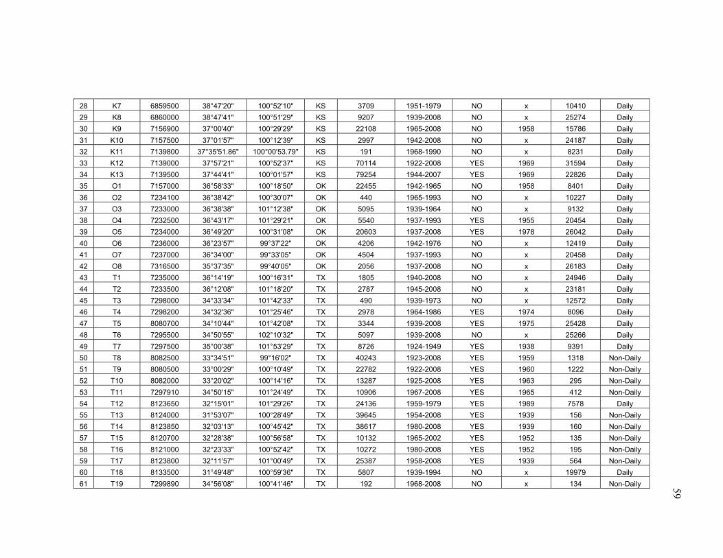
59
28 K7 6859500 38°47'20" 100°52'10" KS 3709 1951-1979 NO x 10410 Daily
29 K8 6860000 38°47'41" 100°51'29" KS 9207 1939-2008 NO x 25274 Daily
30 K9 7156900 37°00'40" 100°29'29" KS 22108 1965-2008 NO 1958 15786 Daily
31 K10 7157500 37°01'57" 100°12'39" KS 2997 1942-2008 NO x 24187 Daily
32 K11 7139800 37°35'51.86" 100°00'53.79" KS 191 1968-1990 NO x 8231 Daily
33 K12 7139000 37°57'21" 100°52'37" KS 70114 1922-2008 YES 1969 31594 Daily
34 K13 7139500 37°44'41" 100°01'57" KS 79254 1944-2007 YES 1969 22826 Daily
35 O1 7157000 36°58'33" 100°18'50" OK 22455 1942-1965 NO 1958 8401 Daily
36 O2 7234100 36°38'42" 100°30'07" OK 440 1965-1993 NO x 10227 Daily
37 O3 7233000 36°38'38" 101°12'38" OK 5095 1939-1964 NO x 9132 Daily
38 O4 7232500 36°43'17" 101°29'21" OK 5540 1937-1993 YES 1955 20454 Daily
39 O5 7234000 36°49'20" 100°31'08" OK 20603 1937-2008 YES 1978 26042 Daily
40 O6 7236000 36°23'57" 99°37'22" OK 4206 1942-1976 NO x 12419 Daily
41 O7 7237000 36°34'00" 99°33'05" OK 4504 1937-1993 NO x 20458 Daily
42 O8 7316500 35°37'35" 99°40'05" OK 2056 1937-2008 NO x 26183 Daily
43 T1 7235000 36°14'19" 100°16'31" TX 1805 1940-2008 NO x 24946 Daily
44 T2 7233500 36°12'08" 101°18'20" TX 2787 1945-2008 NO x 23181 Daily
45 T3 7298000 34°33'34" 101°42'33" TX 490 1939-1973 NO x 12572 Daily
46 T4 7298200 34°32'36" 101°25'46" TX 2978 1964-1986 YES 1974 8096 Daily
47 T5 8080700 34°10'44" 101°42'08" TX 3344 1939-2008 YES 1975 25428 Daily
48 T6 7295500 34°50'55" 102°10'32" TX 5097 1939-2008 NO x 25266 Daily
49 T7 7297500 35°00'38" 101°53'29" TX 8726 1924-1949 YES 1938 9391 Daily
50 T8 8082500 33°34'51" 99°16'02" TX 40243 1923-2008 YES 1959 1318 Non-Daily
51 T9 8080500 33°00'29" 100°10'49" TX 22782 1922-2008 YES 1960 1222 Non-Daily
52 T10 8082000 33°20'02" 100°14'16" TX 13287 1925-2008 YES 1963 295 Non-Daily
53 T11 7297910 34°50'15" 101°24'49" TX 10906 1967-2008 YES 1965 412 Non-Daily
54 T12 8123650 32°15'01" 101°29'26" TX 24136 1959-1979 YES 1989 7578 Daily
55 T13 8124000 31°53'07" 100°28'49" TX 39645 1954-2008 YES 1939 156 Non-Daily
56 T14 8123850 32°03'13" 100°45'42" TX 38617 1980-2008 YES 1939 160 Non-Daily
57 T15 8120700 32°28'38" 100°56'58" TX 10132 1965-2002 YES 1952 135 Non-Daily
58 T16 8121000 32°23'33" 100°52'42" TX 10272 1980-2008 YES 1952 195 Non-Daily
59 T17 8123800 32°11'57" 101°00'49" TX 25387 1958-2008 YES 1939 564 Non-Daily
60 T18 8133500 31°49'48" 100°59'36" TX 5807 1939-1994 NO x 19979 Daily
61 T19 7299890 34°56'08" 100°41'46" TX 192 1968-2008 NO x 134 Non-Daily
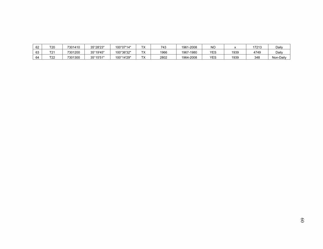
60
62 T20 7301410 35°28'23" 100°07'14" TX 743 1961-2008 NO x 17213 Daily
63 T21 7301200 35°19'45" 100°36'32" TX 1966 1967-1980 YES 1939 4749 Daily
64 T22 7301300 35°15'51" 100°14'29" TX 2802 1964-2008 YES 1939 348 Non-Daily

61
Table 2.3. List of the precipitation sites used in this study.
Precipitation
Sites Site Name State Latitude Longitude
Record
Period
Elevation
(m)
P1 Alliance 1 WNW NE 42°06'36" 102°54'36" 1895-2003
1218
P2 Imperial NE 40°31'12" 101°38'24" 1890-2005
1000
P3 Burlington Col USA CO 39°17'59" 102°17'59" 1918-1989
1271
P4 Cheyenne Wells KS 38°49'12" 102°20'59" 1900-2005
1296
P5 Liberal KS 37°02'59" 100°55'12" 1907-2005
864
P6 Stratford TX 36°21'36" 102°05'24" 1911-2005
1126
P7 Miami TX 35°42'36" 100°38'24" 1905-2005
840
P8 Muleshoe 1 TX 34°14'24" 102°44'24" 1921-2005
1167
P9 Garden City 1 E USA TX 31°53'59" 101°30'00" 1912-1989
802
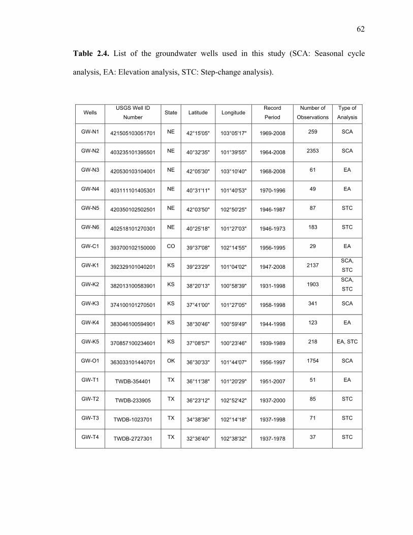
62
Table 2.4. List of the groundwater wells used in this study (SCA: Seasonal cycle
analysis, EA: Elevation analysis, STC: Step-change analysis).
Wells USGS Well ID
Number State Latitude Longitude
Record
Period
Number of
Observations
Type of
Analysis
GW-N1 421505103051701 NE 42°15'05" 103°05'17" 1969-2008 259 SCA
GW-N2 403235101395501 NE 40°32'35" 101°39'55" 1964-2008 2353 SCA
GW-N3 420530103104001 NE 42°05'30" 103°10'40" 1968-2008 61 EA
GW-N4 403111101405301 NE 40°31'11" 101°40'53" 1970-1996 49 EA
GW-N5 420350102502501 NE 42°03'50" 102°50'25" 1946-1987 87 STC
GW-N6 402518101270301 NE 40°25'18" 101°27'03" 1946-1973 183 STC
GW-C1 393700102150000 CO 39°37'08" 102°14'55" 1956-1995 29 EA
GW-K1 392329101040201 KS 39°23'29" 101°04'02" 1947-2008 2137 SCA,
STC
GW-K2 382013100583901 KS 38°20'13" 100°58'39" 1931-1998 1903 SCA,
STC
GW-K3 374100101270501 KS 37°41'00" 101°27'05" 1958-1998 341 SCA
GW-K4 383046100594901 KS 38°30'46" 100°59'49" 1944-1998 123 EA
GW-K5 370857100234601 KS 37°08'57" 100°23'46" 1939-1989 218 EA, STC
GW-O1 363033101440701 OK 36°30'33" 101°44'07" 1956-1997 1754 SCA
GW-T1 TWDB-354401 TX 36°11'38" 101°20'29" 1951-2007 51 EA
GW-T2 TWDB-233905 TX 36°23'12" 102°52'42" 1937-2000 85 STC
GW-T3 TWDB-1023701 TX 34°38'36" 102°14'18" 1937-1998 71 STC
GW-T4 TWDB-2727301 TX 32°36'40" 102°38'32" 1937-1978 37 STC
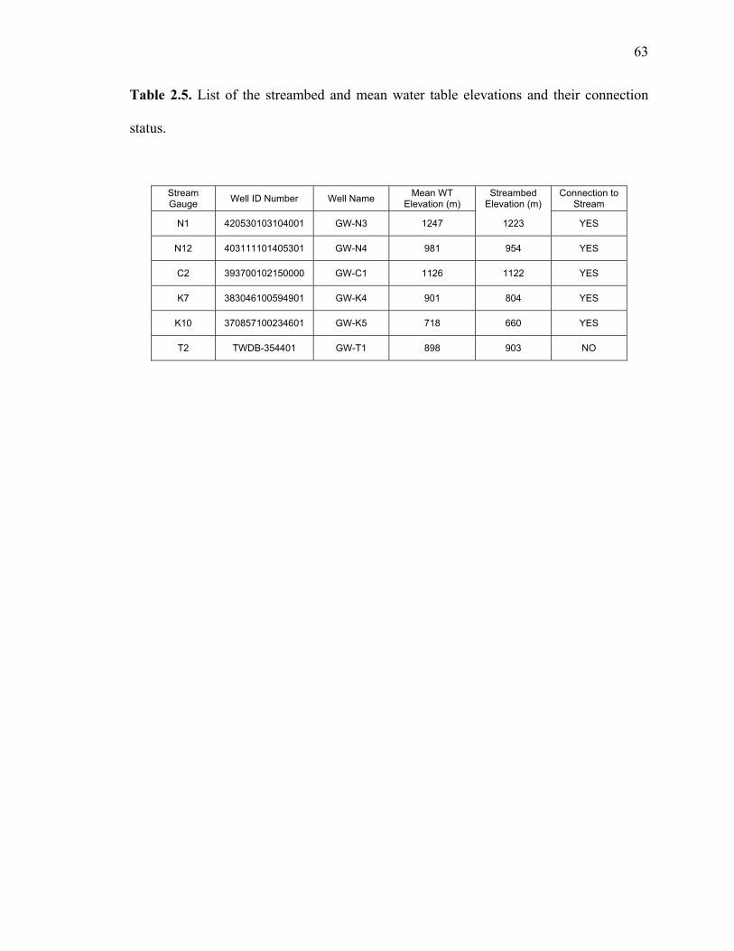
63
Table 2.5. List of the streambed and mean water table elevations and their connection
status.
Stream Gauge
Well ID Number Well Name Mean WT
Elevation (m) Streambed
Elevation (m) Connection to
Stream
N1 420530103104001 GW-N3 1247 1223 YES
N12 403111101405301 GW-N4 981 954 YES
C2 393700102150000 GW-C1 1126 1122 YES
K7 383046100594901 GW-K4 901 804 YES
K10 370857100234601 GW-K5 718 660 YES
T2 TWDB-354401 GW-T1 898 903 NO

64
Table 2.6. Trend test results of mean annual flow, dry-season flow and number of low
flow days (Stream sites in bold represent the ones under the dam effect).
Stream Sites Record Period
Annual Mean Flow Trends
Dry-season Mean Flow Trends
Low-flow Days Trends
1 N1 1946-1994 Decreasing Insignificant Decreasing
2 N2 1946-1991 Decreasing Insignificant Decreasing
3 N3 1945-1991 Decreasing Decreasing Insignificant
4 N4 1930-1991 Decreasing Decreasing Insignificant
5 N5 1935-2008 Decreasing Decreasing Insignificant
6 N6 1932-2008 Decreasing Decreasing Insignificant
7 N7 1940-2008 Decreasing Decreasing Increasing
8 N8 1940-2008 Decreasing Decreasing Insignificant
9 N9 1947-1994 Decreasing Insignificant Insignificant
10 N10 1950-2008 Decreasing Decreasing Increasing
11 N11 1946-1993 Decreasing Decreasing Decreasing
12 N12 1941-1994 Decreasing Decreasing Increasing
13 N13 1946-1993 Decreasing Insignificant Increasing
14 N14 1950-2008 Decreasing Decreasing Increasing
15 N15 1949-1994 Decreasing Decreasing Increasing
16 N16 1935-2008 Decreasing Decreasing Increasing
17 N17 1946-1986 Decreasing Insignificant Decreasing
18 N18 1937-2008 Decreasing Decreasing Increasing
19 C1 1950-1976 Insignificant Insignificant Insignificant
20 C2 1950-1971 Insignificant Insignificant Increasing
21 C3 1946-1986 Decreasing Insignificant Insignificant
22 K1 1959-2008 Decreasing Insignificant Insignificant
23 K2 1946-2008 Decreasing Decreasing Increasing
24 K3 1929-2006 Decreasing Insignificant Insignificant
25 K4 1945-2008 Decreasing Decreasing Insignificant
26 K5 1946-1984 Insignificant Insignificant Increasing
27 K6 1966-1986 Decreasing Insignificant Insignificant
28 K7 1951-1979 Decreasing Insignificant Insignificant
29 K8 1939-2008 Decreasing Decreasing Increasing
30 K9 1965-2008 Decreasing Decreasing Increasing
31 K10 1942-2008 Decreasing Decreasing Decreasing
32 K11 1968-1990 Decreasing Decreasing Increasing
33 K12 1922-2008 Insignificant Insignificant Insignificant

65
34 K13 1944-2007 Decreasing Decreasing Increasing
35 O1 1942-1965 Insignificant Insignificant Decreasing
36 O2 1965-1993 Insignificant Insignificant Insignificant
37 O3 1939-1964 Insignificant Insignificant Insignificant
38 O4 1937-1993 Decreasing Decreasing Increasing
39 O5 1937-2008 Decreasing Decreasing Insignificant
40 O6 1942-1976 Decreasing Insignificant Decreasing
41 O7 1937-1993 Decreasing Decreasing Decreasing
42 O8 1937-2008 Insignificant Insignificant Decreasing
43 T1 1940-2008 Insignificant Insignificant Insignificant
44 T2 1945-2008 Decreasing Insignificant Increasing
45 T3 1939-1973 Insignificant Insignificant Increasing
46 T4 1964-1986 Insignificant Decreasing Increasing
47 T5 1939-2008 Insignificant Insignificant Insignificant
48 T6 1939-2008 Insignificant Insignificant Insignificant
49 T7 1924-1949 Insignificant Insignificant Insignificant
50 T8 1923-2008 Insignificant Insignificant -
51 T9 1922-2008 Insignificant Insignificant -
52 T10 1925-2008 Insignificant Insignificant -
53 T11 1967-2008 Insignificant Insignificant -
54 T12 1959-1979 Insignificant Insignificant Decreasing
55 T13 1954-2008 Insignificant Insignificant -
56 T14 1980-2008 Insignificant Insignificant -
57 T15 1965-2002 Decreasing Insignificant -
58 T16 1980-2008 Insignificant Insignificant -
59 T17 1958-2008 Insignificant Insignificant -
60 T18 1939-1994 Insignificant Insignificant Insignificant
61 T19 1968-2008 Insignificant Insignificant -
62 T20 1961-2008 Insignificant Insignificant Insignificant
63 T21 1967-1980 Insignificant Insignificant Insignificant
64 T22 1964-2008 Insignificant Insignificant -
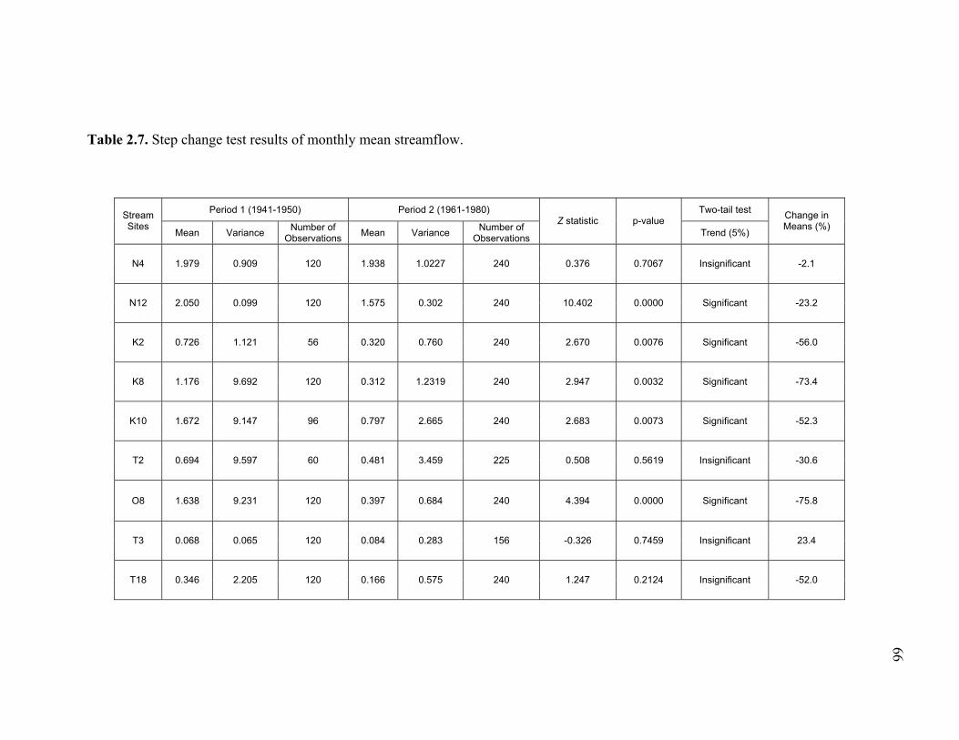
66
Table 2.7. Step change test results of monthly mean streamflow.
Period 1 (1941-1950) Period 2 (1961-1980) Two-tail test Stream Sites
Mean Variance Number of
Observations Mean Variance
Number of Observations
Z statistic p-value Trend (5%)
Change in Means (%)
N4 1.979 0.909 120 1.938 1.0227 240 0.376 0.7067 Insignificant -2.1
N12 2.050 0.099 120 1.575 0.302 240 10.402 0.0000 Significant -23.2
K2 0.726 1.121 56 0.320 0.760 240 2.670 0.0076 Significant -56.0
K8 1.176 9.692 120 0.312 1.2319 240 2.947 0.0032 Significant -73.4
K10 1.672 9.147 96 0.797 2.665 240 2.683 0.0073 Significant -52.3
T2 0.694 9.597 60 0.481 3.459 225 0.508 0.5619 Insignificant -30.6
O8 1.638 9.231 120 0.397 0.684 240 4.394 0.0000 Significant -75.8
T3 0.068 0.065 120 0.084 0.283 156 -0.326 0.7459 Insignificant 23.4
T18 0.346 2.205 120 0.166 0.575 240 1.247 0.2124 Insignificant -52.0

67
Table 2.8. Summarized step-change test results of monthly mean streamflow,
precipitation, and water table elevation.
Precipitation Sites
Annual Trend Results (5%)
Stream Sites
Annual Trend Results (5%)
Groundwater Sites
Annual Trend Results (5%)
P1 Insignificant N4 Insignificant GW-N5 Significant
P2 Insignificant N12 Significant GW-N6 Significant
P3 Significant K2 Significant GW-K1 Significant
P4 Insignificant K8 Significant GW-K2 Significant
P5 Insignificant K10 Significant GW-K5 Significant
P6 Insignificant T2 Insignificant GW-T2 Significant
P7 Significant O8 Significant ? -
P8 Insignificant T3 Insignificant GW-T3 Significant
P9 Insignificant T18 Insignificant GW-T4 Significant
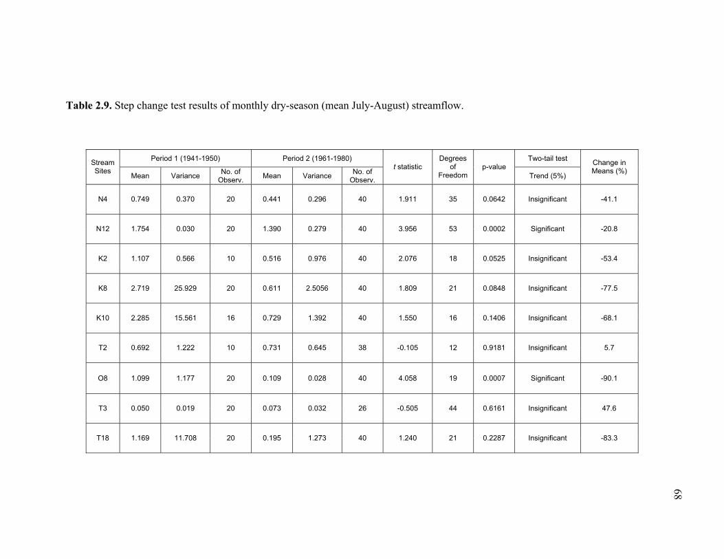
68
Table 2.9. Step change test results of monthly dry-season (mean July-August) streamflow.
Period 1 (1941-1950) Period 2 (1961-1980) Two-tail test Stream Sites
Mean Variance No. of
Observ. Mean Variance
No. of Observ.
t statistic Degrees
of Freedom
p-value Trend (5%)
Change in Means (%)
N4 0.749 0.370 20 0.441 0.296 40 1.911 35 0.0642 Insignificant -41.1
N12 1.754 0.030 20 1.390 0.279 40 3.956 53 0.0002 Significant -20.8
K2 1.107 0.566 10 0.516 0.976 40 2.076 18 0.0525 Insignificant -53.4
K8 2.719 25.929 20 0.611 2.5056 40 1.809 21 0.0848 Insignificant -77.5
K10 2.285 15.561 16 0.729 1.392 40 1.550 16 0.1406 Insignificant -68.1
T2 0.692 1.222 10 0.731 0.645 38 -0.105 12 0.9181 Insignificant 5.7
O8 1.099 1.177 20 0.109 0.028 40 4.058 19 0.0007 Significant -90.1
T3 0.050 0.019 20 0.073 0.032 26 -0.505 44 0.6161 Insignificant 47.6
T18 1.169 11.708 20 0.195 1.273 40 1.240 21 0.2287 Insignificant -83.3

69
Table 2.10. Summarized step change test results of monthly mean dry-season
streamflow, precipitation, and water table elevation.
Precipitation Sites
Dry-season Trend Results (5%)
Stream Sites
Dry-season Trend Results (5%)
Groundwater Sites
Dry-season Trend Results
(5%)
P1 Insignificant N4 Insignificant GW-N5 NaN
P2 Insignificant N12 Significant GW-N6 Insignificant
P3 Significant K2 Insignificant GW-K1 Significant
P4 Insignificant K8 Insignificant GW-K2 Significant
P5 Insignificant K10 Insignificant GW-K5 NaN
P6 Insignificant T2 Insignificant GW-T2 NaN
P7 Insignificant O8 Significant ?
P8 Insignificant T3 Insignificant GW-T3 NaN
P9 Insignificant T18 Insignificant GW-T4 NaN
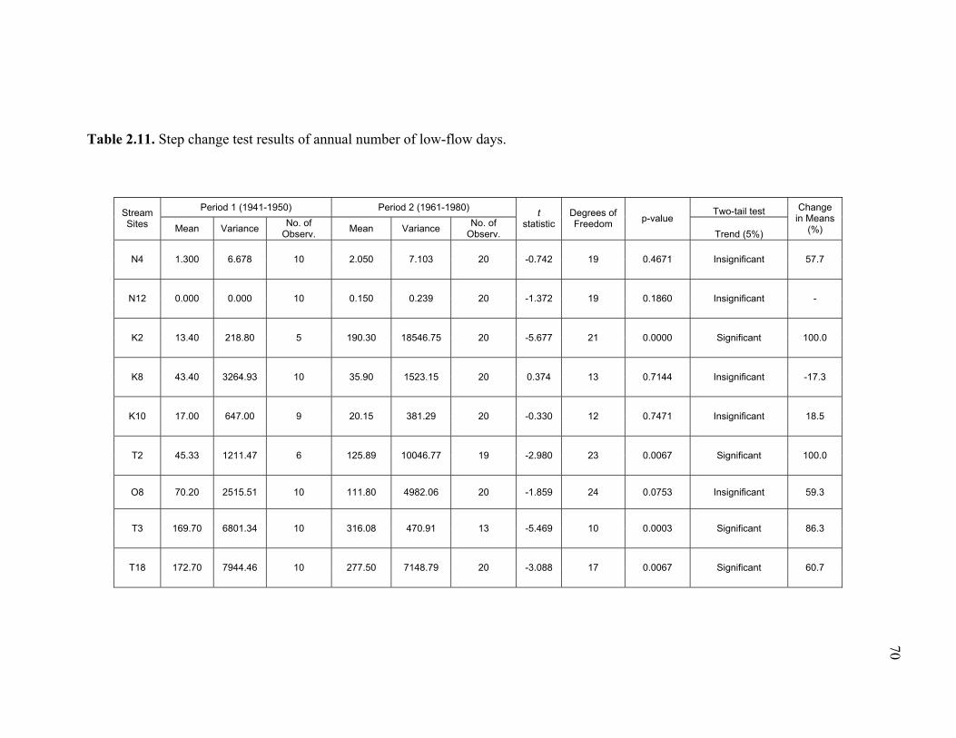
70
Table 2.11. Step change test results of annual number of low-flow days.
Period 1 (1941-1950) Period 2 (1961-1980) Two-tail test Stream Sites Mean Variance
No. of Observ.
Mean Variance No. of
Observ.
t statistic
Degrees of Freedom
p-value
Trend (5%)
Change in Means
(%)
N4 1.300 6.678 10 2.050 7.103 20 -0.742 19 0.4671 Insignificant 57.7
N12 0.000 0.000 10 0.150 0.239 20 -1.372 19 0.1860 Insignificant -
K2 13.40 218.80 5 190.30 18546.75 20 -5.677 21 0.0000 Significant 100.0
K8 43.40 3264.93 10 35.90 1523.15 20 0.374 13 0.7144 Insignificant -17.3
K10 17.00 647.00 9 20.15 381.29 20 -0.330 12 0.7471 Insignificant 18.5
T2 45.33 1211.47 6 125.89 10046.77 19 -2.980 23 0.0067 Significant 100.0
O8 70.20 2515.51 10 111.80 4982.06 20 -1.859 24 0.0753 Insignificant 59.3
T3 169.70 6801.34 10 316.08 470.91 13 -5.469 10 0.0003 Significant 86.3
T18 172.70 7944.46 10 277.50 7148.79 20 -3.088 17 0.0067 Significant 60.7
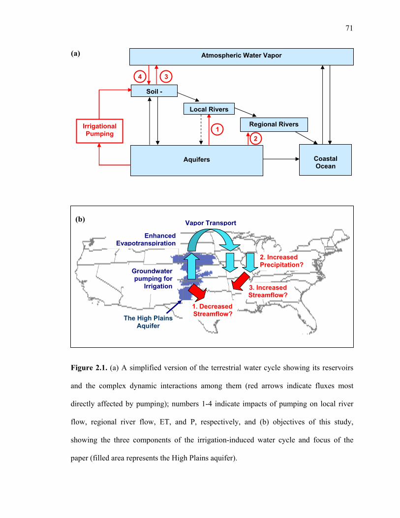
71
Figure 2.1. (a) A simplified version of the terrestrial water cycle showing its reservoirs
and the complex dynamic interactions among them (red arrows indicate fluxes most
directly affected by pumping); numbers 1-4 indicate impacts of pumping on local river
flow, regional river flow, ET, and P, respectively, and (b) objectives of this study,
showing the three components of the irrigation-induced water cycle and focus of the
paper (filled area represents the High Plains aquifer).
Regional Rivers
Atmospheric Water Vapor
Soil -
Local Rivers
Coastal Ocean
Aquifers
Irrigational Pumping 1
2
34
(a)
1. Decreased Streamflow?
3. Increased Streamflow?
Groundwater pumping for
Irrigation
Enhanced Evapotranspiration
2. Increased Precipitation?
(b)
The High Plains Aquifer
Vapor Transport
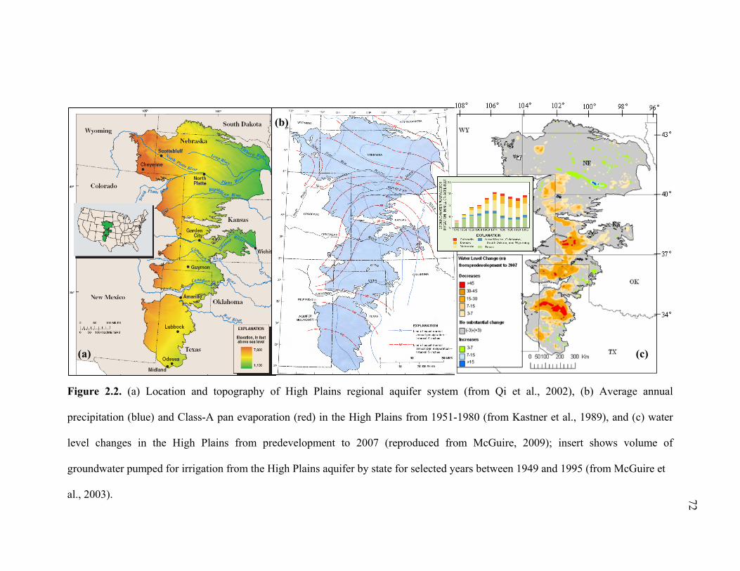
72
Figure 2.2. (a) Location and topography of High Plains regional aquifer system (from Qi et al., 2002), (b) Average annual
precipitation (blue) and Class-A pan evaporation (red) in the High Plains from 1951-1980 (from Kastner et al., 1989), and (c) water
level changes in the High Plains from predevelopment to 2007 (reproduced from McGuire, 2009); insert shows volume of
groundwater pumped for irrigation from the High Plains aquifer by state for selected years between 1949 and 1995 (from McGuire et
al., 2003).
(a)
(b)
(c)

73
Figure 2.3. Map with all the hydrologic sites examined for this study. Base map
(McGuire, 2009) shows the water-level changes in the High Plains aquifer from pre-
development (i.e. before irrigation) to 2007.
Water Level Change (m)
Decreases
No substantial change
Increases
(-3)-(+3)
from predevelopment to 2007
3-7
7-15
>15
>45
30-45
15-30
7-15
3-7
104 102106 108 100 98 96
40
37
43
34

74
Figure 2.4. Locations of the streamflow, groundwater and precipitation sites used in the
step-change analysis.
40
37
43
34
104 102106 108 100 98 96
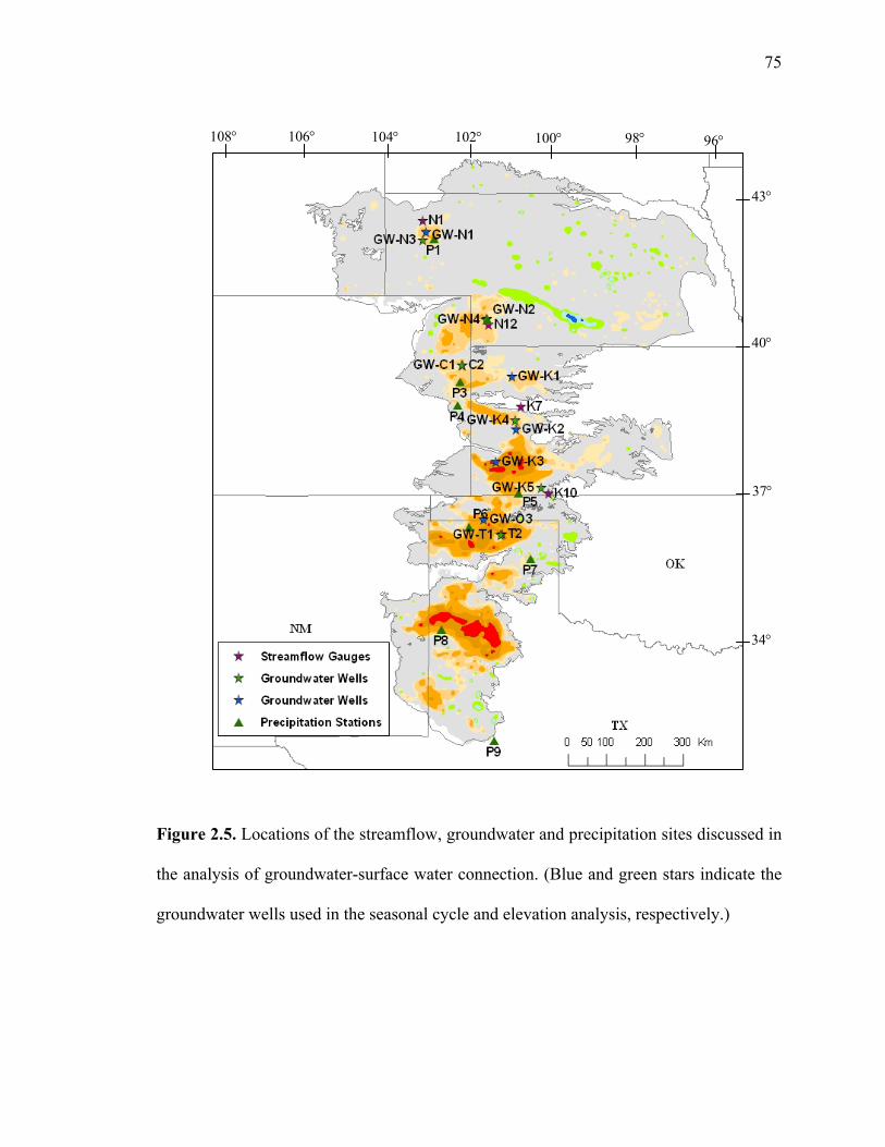
75
Figure 2.5. Locations of the streamflow, groundwater and precipitation sites discussed in
the analysis of groundwater-surface water connection. (Blue and green stars indicate the
groundwater wells used in the seasonal cycle and elevation analysis, respectively.)
104 102106 108 100 98 96
40
37
43
34
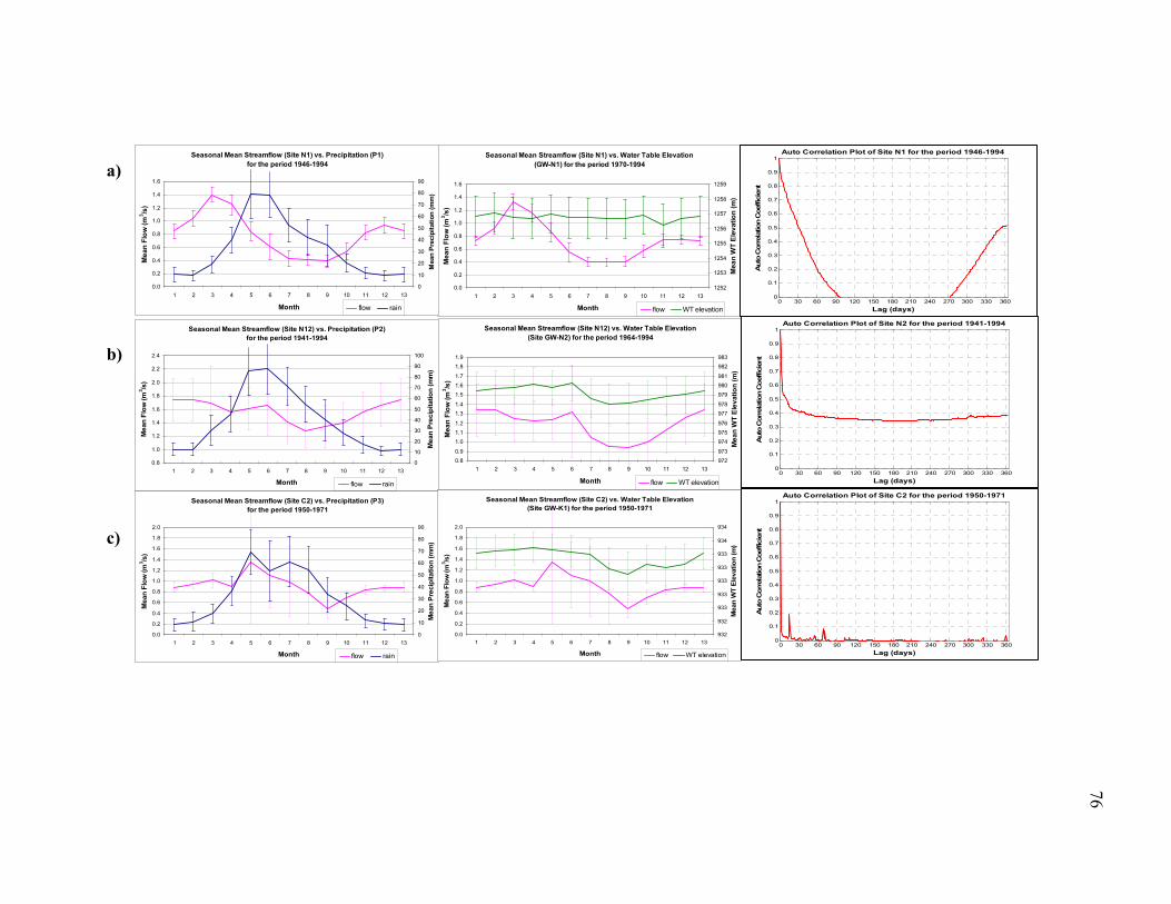
76
a)
b)
c)
Seasonal Mean Streamflow (Site N12) vs. Precipitation (P2) for the period 1941-1994
0.8
1.0
1.2
1.4
1.6
1.8
2.0
2.2
2.4
1 2 3 4 5 6 7 8 9 10 11 12 13
Month
Mea
n Fl
ow (m
3 /s)
0
10
20
30
40
50
60
70
80
90
100
Mea
n Pr
ecip
itatio
n (m
m)
flow rain
Seasonal Mean Streamflow (Site N12) vs. Water Table Elevation (Site GW-N2) for the period 1964-1994
0.8
0.9
1.0
1.1
1.2
1.3
1.4
1.5
1.6
1.7
1.8
1.9
1 2 3 4 5 6 7 8 9 10 11 12 13
Month
Mea
n Fl
ow (m
3 /s)
972
973
974
975
976
977
978
979
980
981
982
983
Mea
n W
T E
leva
tion
(m)
flow WT elevation
0 30 60 90 120 150 180 210 240 270 300 330 3600
0.1
0.2
0.3
0.4
0.5
0.6
0.7
0.8
0.9
1
Lag (days)
Aut
o C
orre
latio
n C
oeffi
cien
t
Auto Correlation Plot of Site N2 for the period 1941-1994
Seasonal Mean Streamflow (Site C2) vs. Precipitation (P3) for the period 1950-1971
0.0
0.2
0.4
0.6
0.8
1.0
1.2
1.4
1.6
1.8
2.0
1 2 3 4 5 6 7 8 9 10 11 12 13
Month
Mea
n Fl
ow (m
3 /s)
0
10
20
30
40
50
60
70
80
90
Mea
n Pr
ecip
itatio
n (m
m)
flow rain
Seasonal Mean Streamflow (Site C2) vs. Water Table Elevation (Site GW-K1) for the period 1950-1971
0.0
0.2
0.4
0.6
0.8
1.0
1.2
1.4
1.6
1.8
2.0
1 2 3 4 5 6 7 8 9 10 11 12 13
Month
Mea
n Fl
ow (m
3 /s)
932
932
933
933
933
933
933
934
934
Mea
n W
T El
evat
ion
(m)
flow WT elevation
0 30 60 90 120 150 180 210 240 270 300 330 3600
0.1
0.2
0.3
0.4
0.5
0.6
0.7
0.8
0.9
1
Lag (days)
Aut
o C
orre
latio
n C
oeffi
cien
t
Auto Correlation Plot of Site C2 for the period 1950-1971
Seasonal Mean Streamflow (Site N1) vs. Water Table Elevation (GW-N1) for the period 1970-1994
0.0
0.2
0.4
0.6
0.8
1.0
1.2
1.4
1.6
1 2 3 4 5 6 7 8 9 10 11 12 13
Month
Mea
n Fl
ow (m
3 /s)
1252
1253
1254
1255
1256
1257
1258
1259
Mea
n W
T El
evat
ion
(m)
flow WT elevation
Seasonal Mean Streamflow (Site N1) vs. Precipitation (P1) for the period 1946-1994
0.0
0.2
0.4
0.6
0.8
1.0
1.2
1.4
1.6
1 2 3 4 5 6 7 8 9 10 11 12 13
Month
Mea
n Fl
ow (m
3 /s)
0
10
20
30
40
50
60
70
80
90
Mea
n Pr
ecip
itatio
n (m
m)
flow rain0 30 60 90 120 150 180 210 240 270 300 330 360
0
0.1
0.2
0.3
0.4
0.5
0.6
0.7
0.8
0.9
1
Lag (days)
Aut
o C
orre
latio
n C
oeffi
cien
t
Auto Correlation Plot of Site N1 for the period 1946-1994

77
d)
e)
f)
Figure 2.6. Mean seasonal cycles of streamflow vs. local precipitation, streamflow vs. groundwater table elevation, and
autocorrelation plots for the analyzed sites. (Error bars represent one standard deviation.)
Seasonal Mean Streamflow (Site K10) vs. Precipitation (P5) for the period 1942-2005
0.0
0.2
0.4
0.6
0.8
1.0
1.2
1.4
1.6
1.8
2.0
2.2
1 2 3 4 5 6 7 8 9 10 11 12 13
Month
Mea
n Fl
ow (m
3 /s)
0
10
20
30
40
50
60
70
80
90
Mea
n Pr
ecip
itatio
n (m
m)
flow rain
Seasonal Mean Streamflow (Site K10) vs. Water Table Elevation (Site GW-K3) for the period 1958-1998
0.0
0.2
0.4
0.6
0.8
1.0
1.2
1.4
1.6
1.8
2.0
2.2
1 2 3 4 5 6 7 8 9 10 11 12 13
Month
Mea
n Fl
ow (m
3 /s)
900
902
904
906
908
910
912
914
916
918
920
922
Mea
n W
T El
evat
ion
(m)
flow WT elevation0 30 60 90 120 150 180 210 240 270 300 330 360
0
0.1
0.2
0.3
0.4
0.5
0.6
0.7
0.8
0.9
1
Lag (days)
Aut
o C
orre
latio
n C
oeffi
cien
t
Auto Correlation Plot of Site K10 for the period 1942-2008
Seasonal Mean Streamflow (Site T2) vs. Precipitation (P6) for the period 1945-1979
0.0
0.2
0.4
0.6
0.8
1.0
1.2
1.4
1.6
1.8
2.0
2.2
2.4
1 2 3 4 5 6 7 8 9 10 11 12 13
Month
Mea
n Fl
ow (m
3 /s)
0
10
20
30
40
50
60
70
80
90
Mea
n Pr
ecip
itatio
n (m
m)
flow rain
Seasonal Mean Streamflow (Site T2) vs. Water Table Elevation (Site GW-O1) for the period 1957-1979
0.0
0.2
0.4
0.6
0.8
1.0
1.2
1.4
1.6
1.8
2.0
2.2
2.4
1 2 3 4 5 6 7 8 9 10 11 12 13
Month
Mea
n Fl
ow (m
3 /s)
986.0
986.5
987.0
987.5
988.0
988.5
989.0
989.5
990.0
Mea
n W
T El
evat
ion
(m)
flow WT elevation0 30 60 90 120 150 180 210 240 270 300 330 360
0
0.1
0.2
0.3
0.4
0.5
0.6
0.7
0.8
0.9
1
Lag (days)
Aut
o C
orre
latio
n C
oeffi
cien
t
Auto Correlation Plot of Site T2 for the period 1945-1979
Seasonal Mean Streamflow (Site K7) vs. Precipitation (P4) for the period 1951-1979
0.00.20.40.6
0.81.01.21.41.61.82.0
2.22.42.62.8
1 2 3 4 5 6 7 8 9 10 11 12 13
Month
Mea
n Fl
ow (m
3 /s)
0
10
20
30
40
50
60
70
80
90
Mea
n P
reci
pita
tion
(mm
)
flow rain
Seasonal Mean Streamflow (Site K7) vs. Water Table Elevation (Site GW-K2) for the period 1951-1979
0.0
0.20.4
0.6
0.8
1.01.2
1.4
1.61.8
2.0
2.2
2.42.6
2.8
1 2 3 4 5 6 7 8 9 10 11 12 13
Month
Mea
n Fl
ow (m
3 /s)
877
878
879
880
881
882
883
Mea
n W
T El
evat
ion
(m)
flow WT elevation
0 30 60 90 120 150 180 210 240 270 300 330 3600
0.1
0.2
0.3
0.4
0.5
0.6
0.7
0.8
0.9
1
Lag (days)
Aut
o C
orre
latio
n C
oeffi
cien
t
Auto Correlation Plot of Site K7 for the period 1951-1979
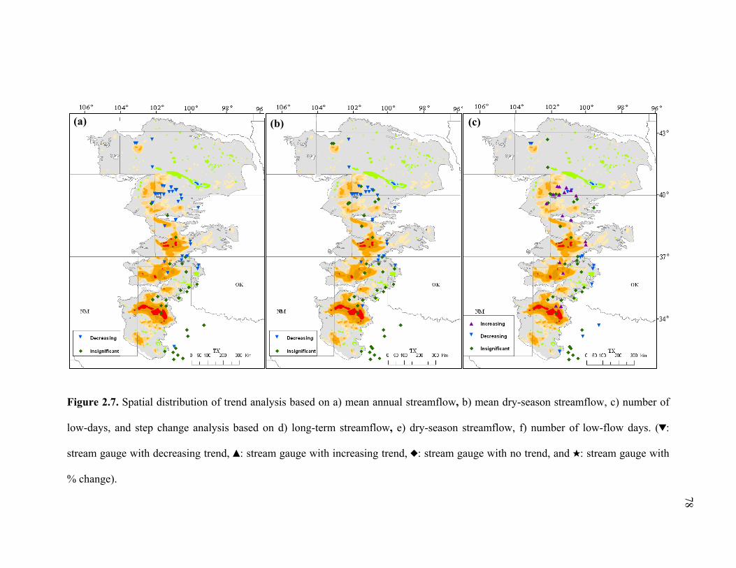
78
Figure 2.7. Spatial distribution of trend analysis based on a) mean annual streamflow, b) mean dry-season streamflow, c) number of
low-days, and step change analysis based on d) long-term streamflow, e) dry-season streamflow, f) number of low-flow days. (&:
stream gauge with decreasing trend, %: stream gauge with increasing trend, ": stream gauge with no trend, and $: stream gauge with
% change).
(a) (b) (c)
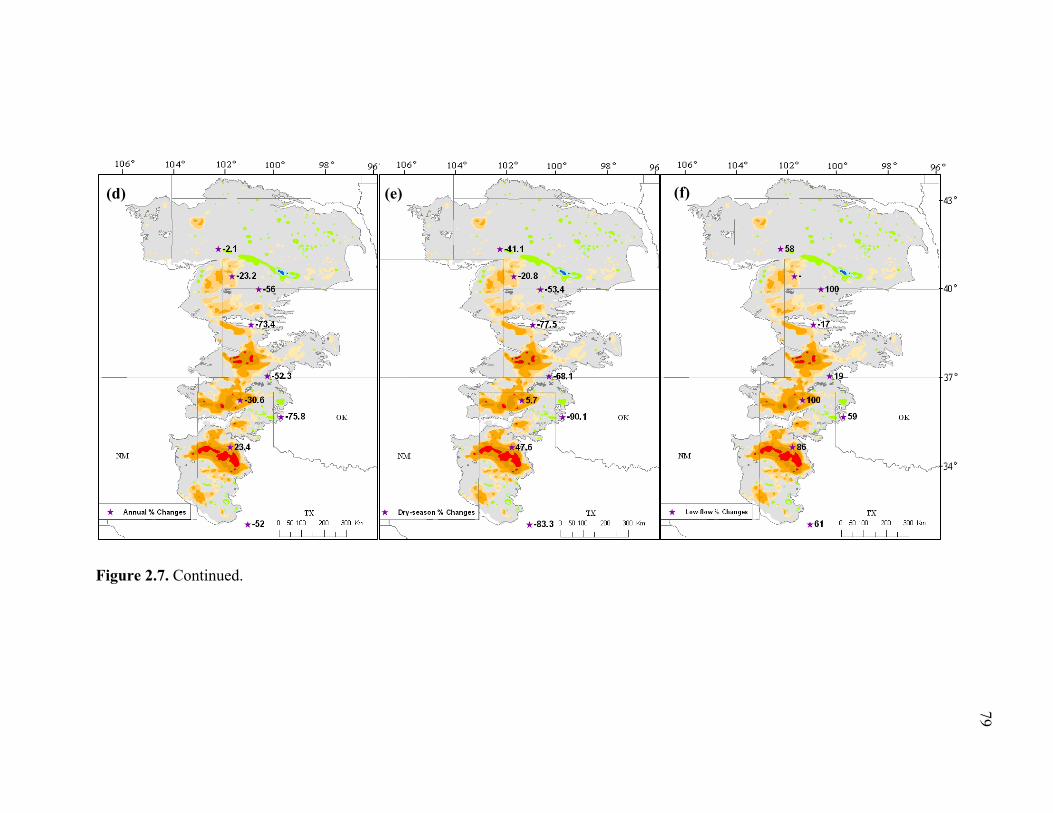
79
Figure 2.7. Continued.
(d) (e) (f)

80
Figure 2.8. Time series of mean July-August flow at the gauges that fail to show significant trends in dry-season flow but have
decreasing trends in the mean annual flow.
Mean Dry-season Streamflow Variability
0
1
2
3
4
5
6
7
8
9
19291932193519381941194419471950195319561959196219651968197119741977198019831986198919921995199820012004
Time (years)
Mea
n Ju
ly-A
ugus
t Flo
w (m
3 /s)
N1
N9
N17
K1
K3
K6
K7
O6
T2
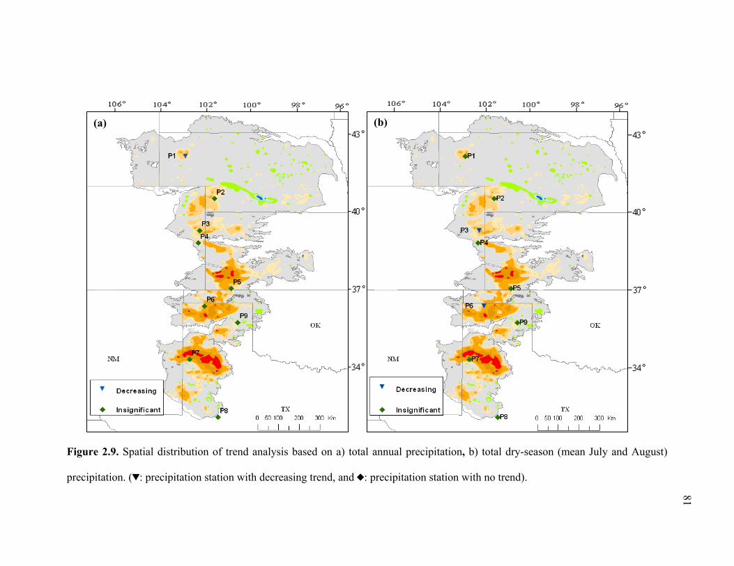
81
Figure 2.9. Spatial distribution of trend analysis based on a) total annual precipitation, b) total dry-season (mean July and August)
precipitation. (&: precipitation station with decreasing trend, and ": precipitation station with no trend).
(a) (b)
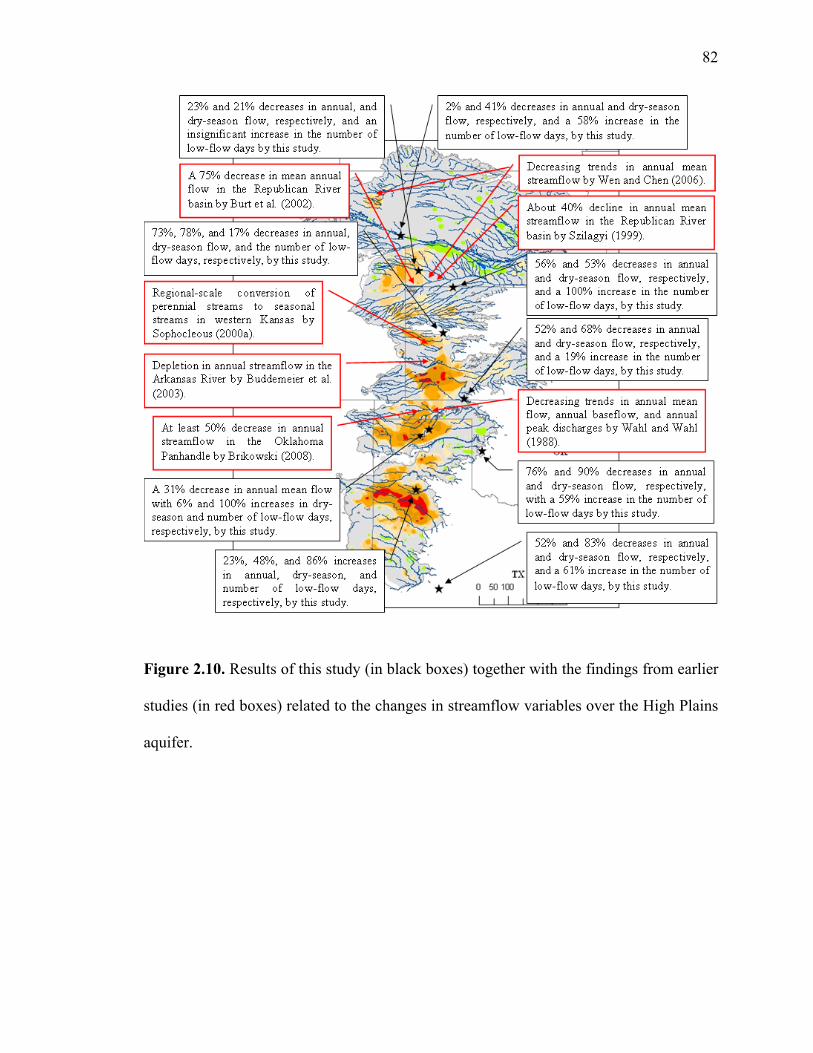
82
Figure 2.10. Results of this study (in black boxes) together with the findings from earlier
studies (in red boxes) related to the changes in streamflow variables over the High Plains
aquifer.
83
Chapter 3
Possible Link between Irrigation in the US High Plains and Increased Summer
Streamflow in the Midwest
Abstract
Earlier we presented evidence that higher evapotranspiration (ET) associated with
irrigation in the US High Plains has likely caused an increased downwind precipitation
(P). July P over the Midwest increased by 20-30% from pre-irrigation (1900-1950) to the
post-irrigation (1950-2000) period. In this study, we test the hypothesis that the increased
July P has had hydrologic consequences, possibly increasing groundwater storage and
streamflow. Seasonal analyses of hydrologic variables over Illinois suggest that the water
table and streamflow response lags P-ET by 1-2 months, indicating August-September as
the months when the increased July P may be detected. We analyzed long-term
observations of water table depth at 10 wells in Illinois and streamflow at 46 gauges in
Illinois-Ohio Basins. The Mann-Kendall test suggests field-significant increases in
groundwater storage and streamflow in August-September over the period of irrigation
expansion. Examination of soil moisture response to present-day above-normal July P
suggests that the increased July P can reach the water table in normal to wet years. Mann-
Kendall test results suggest no statistically significant changes in pan evaporation and

84
atmospheric vapor pressure deficit. Other studies give evidence of increased ET from
increased P in the region. By ruling out ET reduction, we suggest that the observed
increase in groundwater storage and streamflow in the Midwest is linked to the increased
July precipitation attributed to High Plains’ irrigation. We note that the increases in late-
summer streamflow are rather small when placed in the context of seasonal dynamics, but
they are conceptually important in that they point to a different cause of change.

85
1. Introduction
Groundwater pumping for irrigation in the US High Plains began to accelerate in
the 1940s (Fig. 3.1a), and by the mid 1980s, groundwater levels had declined by >30 m
over much of the High Plains (Fig. 3.1b) (McGuire, 2009). The decades-long and
regional-scale water transfer, from the groundwater reservoir to the soil moisture
reservoir in the warm season, has likely influenced the region’s hydrology and climate.
Moreover, this influence may not have been confined to the High Plains itself, but
propagated downwind through the atmospheric vapor transport pathways, and down-
gradient through the river and groundwater pathways. We hypothesize that, first, the
large groundwater decline has led to reduced streamflow in the High Plains region-wide,
particularly where groundwater is a source for streamflow; second, because irrigation
drastically increases warm season evapotranspiration (ET), it has increased vapor export
and possibly downwind precipitation (P); third, such increased downwind P has altered
the land hydrology over the receiving region, far away from the High Plains where the
change originated. Fig. 3.1c schematically illustrates these hypotheses: 1) reduced
streamflow in the High Plains, 2) increased downwind P, and 3) increased downwind ET
and streamflow.
In an earlier paper (Kustu et al., 2010), we tested the first hypothesis. That
groundwater pumping in the High Plains reduced streamflow was not a new idea; there
had been many reports in the literature on the subject (see detailed review by Kustu et al.,
2010), but they focused on specific areas and applied different methods of analysis,
leaving large spatial gaps and making a regional comparison and synthesis difficult. For
86
example, strong climatic and hydrologic gradients from northern to southern High Plains
are well documented; in the north (e.g. Nebraska), the cooler and moister climate, the
sandy soil and river beds, and the naturally high water table, point to groundwater as a
main source for streamflow, and that changes in the former can directly influence the
latter; in the south (e.g., Texas), the warm and dry climate, the dominance of summer
thunderstorms and surface runoff, and the naturally deep water table, indicate that the
water table may lie below local river beds, and hence pumping may have little effect on
local streamflow (but it may affect regional streams fed by regional groundwater
convergence further down-gradient). To achieve this regional synthesis, we analyzed the
entire groundwater and streamflow records of the US Geologic Survey (USGS). Our
results filled large spatial gaps between previously studied areas and suggest that, indeed,
decreases in annual and dry-season streamflow, and increase in the frequency of low-
flows, are more pronounced in the northwestern part of the High Plains.
In our second study (DeAngelis et al., 2010), we tested the second hypothesis that
irrigation in the High Plains, through increased ET and vapor export, may influence
downwind precipitation. The idea that irrigation can affect rainfall is not new either (see
detailed review by DeAngelis et al. 2010), but earlier studies focused on local P recycling
and were based on short-term observations or model experiments. It is now well
recognized that land surface wetness has a large impact on downwind precipitation (e.g.,
Dominguez et al., 2009; van der Ent et al., 2010), and a recent global modeling study
(Puma and Cook, 2010) reports larger downwind than local increases in precipitation due
to irrigation. In the US, it is well understood that the strong winds of the Great Plains
Low Level Jet (Weaver et al., 2009) (see wind vectors in Fig. 3.2a), peaking in the warm

87
season, connect the High Plains (Region 1, Fig. 3.2a) to its downwind regions to the
northeast. Meanwhile, hundreds of station precipitation records exist in the central US
dating back to at least the early 1930s. A study based on these long-term precipitation
observations with an emphasis on downwind climatic impacts had been lacking. To fill in
this knowledge gap, we analyzed 865 long-term station records, over and downwind of
the High Plains (the three regions in Fig. 3.2a), for signals of change. The observations,
combined with a Lagrangian vapor tracking analysis to trace the fate of the High Plains
ET, revealed evidence that irrigation in the High Plains has led to increased downwind
precipitation, particularly over the Midwest (Region 3, Fig. 3.2a) in the month of July,
the peak month of irrigation and peak month of wind speed in the Great Plains Low Level
Jet (Weaver et al., 2009).
In this paper, we test our third hypothesis that the irrigation-enhanced July
precipitation over the Midwest has had hydrologic consequences. Precipitation is a key
driver of land hydrology, and changes in P will propagate through the various hydrologic
pathways: canopy interception, surface runoff, infiltration, soil and plant ET, water table
recharge, and groundwater discharge into streams. The noticeable increase in July P from
the first to the second half of the century (Fig. 3.2b) likely manifested itself in one or
more of these hydrologic variables. In this paper, we analyze available observations of
these hydrologic variables to search for signals of change that may be attributable to the
increased July precipitation.
In Section 2, we discuss the dominant hydrologic pathways in the region and the
associated time scales whereby precipitation propagates through land hydrology. In
Section 3, we analyze long-term water table, streamflow, soil moisture, air temperature

88
and pan evaporation time series. In Section 4, we discuss the implications of the work
and future research to improve our understanding of hydrologic-climatic interactions in
the context of climate variability and change, and land use or water use changes.
2. Hydrologic Features of the Study Area
The study area is centered over the states of Illinois and Indiana (Fig. 3.2a, green
box) where July precipitation increased by 10-30% from the first to the second half of the
century. The change occurred near the midcentury (Fig. 3.2b), after which the means and
lows all increased and extreme dry periods have been absent. The questions are, how
does such a change in July P (hereafter referred to as July ΔP) propagate through land
hydrology, and can we detect its signal in historically observed hydrologic variables such
as water table depth and streamflow?
As precipitation increases, the vegetation and the near surface soils are the first to
sense it, and if ET is water-limited, ΔP will likely engender increased ET, leaving no
trace in groundwater and streamflow (historically-observed). However, if ET is energy-
limited, then ΔP may infiltrate deeper and recharge the groundwater, leaving a signature
in groundwater and river flow. It may also take the route of increased surface runoff if ΔP
is in the form of higher storm intensity.
To explore the possible partition of ΔP into increased ET (not observed) vs.
groundwater storage and streamflow (observed), we examine the seasonality of land
hydrology in the region. Illinois has one of the best hydrologic monitoring networks in
the world, including soil moisture beginning in 1981 (Hollinger and Isard, 1994) and
89
shallow water table in the late 1950s (Illinois State Water Survey, or ISWS). Although
they began after the initial irrigation expansion, the water table records cover a good
portion of the period. In addition, soil moisture and water table observations provide
essential insight into the cascading of P signals through the hydrologic stores and the
associated time scales.
Fig. 3.3a plots the seasonal cycle of observed P, estimated ET and observed
streamflow (the fluxes), and Fig. 3.3b plots the seasonal cycle of the observed top 2 m
soil moisture (SM) and water table depth (WTD) (the states), averaged over the state of
Illinois and the period of 1983-1995. The data in Fig. 3.3 is directly taken from Eltahir
and Yeh (1999), a seminal study on the hydrologic linkages in the region, where the ET is
the mean of two independent estimates, one based on atmospheric vapor convergence and
the other on soil water budget analysis (Yeh et al., 1998). We note the following:
First, ET flux, with its large seasonal swings, dominates the seasonal dynamics,
exceeding P in May through August. In July, P accounts for 80% of ET, suggesting a net
soil water deficit (P-ET<0). Long-term mean July pan evaporation in central Illinois is
227 mm (as shown later in Fig. 3.10b and Table 3.6), suggesting that the 122 mm ET
here is below potential, and that a July ΔP of ~20% may directly translate into increased
July ET. However, if higher storm intensity accounts for ΔP, it would lead to increased
infiltration-excess surface runoff, leaving a signature in streamflow. Since surface runoff
responds to rainfall quickly, the signature in streamflow would be found in the same
month (July). If ΔP represents longer periods of rainfall, it would increase infiltration into
the soil.
90
Second, the top 2 m soil moisture closely follows the P-ET cycle, with the best
correlation obtained at the 1-month lag (Fig. 3.4a). That is, the top 2 m soil moisture as a
whole responds to climate forcing one month later, although the shallow soils may
respond in the same month. Therefore the signal of ΔP is likely found in July (at shallow
depths) and August (at deeper depths) in the soil moisture records.
Third, the water table cycle closely follows the soil moisture cycle, with the best
correlation obtained at the 1-month lag (Fig. 3.4b). That is, the groundwater on average is
recharged one month after the soil moisture is replenished. This suggests that the signal
of ΔP is likely found in the groundwater records (if at all) in August and September.
Fourth, groundwater fluctuations are closely linked to streamflow. The
streamflow seasonal cycle is mostly in phase (0 lag) with that of the water table depth
(Fig. 3.4c). Eltahir and Yeh (1999) estimated that surface runoff explains <10% of
streamflow variations and accounts for <25% of streamflow, leaving groundwater as the
main source and driver of monthly and seasonal dynamics. This suggests that the July ΔP
signal would find expressions (if at all) in August and September streamflow.
The above analysis is summarized in Fig. 3.4d with the expected lag-times of the
relevant hydrologic variables indicated. The above discussion helps us focus our
subsequent analysis on relevant hydrologic variables and at relevant time scales.
3. Signals of Increased July P in the Observed Hydrologic Variables
Fig. 3.5 gives the mean Region 3 (Fig. 3.2a) precipitation time series (shown as 5-
yr moving average to bring out long-term variabilities) for May-September, based on 316

91
station monthly data from the NCDC (National Climate Data Center,
http://www.ncdc.noaa.gov/oa/ncdc.html). They are shown here because the signal of May
and June P may be present in July and August water table level and streamflow. Over the
period of irrigation expansion (1940-1980, shaded), there is a slight decline in May and
June, a step-like increase at mid-century in July, a rise in late 1970s in August, and no
apparent trend in September. Of the hydrologic variables in Fig. 3.4d, only the
groundwater level and streamflow are observed over the period of interest (1940-1980),
and we start our analysis with these observations.
3.1. Changes in Water Table Depth
Water table observations, dating back to the 1950s, are obtained from USGS at
one site (all others began in the late 1980s) at ~10 day steps, and at nine sites from the
ISWS WARM network (Water and Atmosphere Resource Monitoring,
http://www.isws.illinois.edu/warm/sgwdata/wells.aspx) at monthly steps. All these long-
term observations are in the state of Illinois; no historic groundwater data could be found
in Indiana where the largest July ΔP was observed (Fig. 3.2a). The well locations are
shown in Fig. 3.6a (orange and green) with site information given in Table 3.1 (first
block; the rest had shorter records and used for later analyses). Monthly water table
depths at these 10 sites are plotted in Fig. 3.7 for July-September.
In July, more sites showed an upward trend despite the flat or downward trend in
May and June P. In August and September, the upward trend is more apparent. Table 3.2
gives the result of the statistical test for water table trends in July to September over the
92
period of 1940-1980, using the non-parametric Mann-Kendall test (Mann, 1945; Kendall,
1975). Eight of the 10 sites show a rising trend in the July water table, but it is
statistically significant (at 5% level, or p<0.05, shown in bold) at only two sites, and one
site (W191) has a significant falling trend. In August and September, the number of sites
with significant rising trends increased, consistent with our expectation that if the signal
of ΔP is to be detected in the groundwater, it would be in August and September. The
decreasing trends at W61 (August) and W191 (August-September) are unexplained.
We also evaluate the field significance of the trend test results, which is necessary
when assessing regional trends at multiple sites (e.g. Livezey and Chen, 1983;
Lettenmaier et al., 1994; Douglas et al., 2000; Yue and Wang, 2002; Renard et al., 2008;
and Khaliq et al., 2009). Field significance (α) is the combined significance of N tests; if
the percentage of significant results is greater than α, then the results are said to be field
significant. Two methods can be used. If the sites are spatially independent, α follows the
binomial distribution. The wells used for the trend analysis (orange and green, Fig. 3.6a)
are isolated from one another by several streams, and we consider them hydrologically
independent (e.g., land use change or pumping near one well will not affect another). The
binomial test (Livezey and Chen, 1983) indicates that the water table trends are field
significant at the 5% level in August and September, but not in July (they might have
occurred by chance). If the multiple sites are not independent, then the Regional
Kendall’s S test (Douglas et al., 2000) is appropriate, results of which suggest that the
water table trends are not field significant in any of the months.
3.2. Changes in Streamflow
93
Streamflow records were obtained from the USGS National Water Information
System (NWIS) database (http://nwis.waterdata.usgs.gov/nwis/sw) for a total of 1,428
gauges in the Ohio and 343 in the Illinois River basin. We selected 46 gauges (24 in the
Ohio and 22 in the Illinois basin) for this study according to the following criteria. First,
they are located in areas where more than 10% of July ΔP is detected (see Fig. 3.2a).
Second, their records cover at least 30 years, starting no later than 1941 and ending no
earlier than 1970. Third, the streams are not affected by reservoirs which cause
significant changes in streamflow, especially during summer months, making attributions
of change difficult (Yang et al., 2004; Haddeland et al., 2006b); but those gauges where
regulation began after 1970 are retained with the data after removed. Fourth, these
streams do not drain into one another, so that each gauge represents an independent
measurement; if one drains into another, the larger basin is retained. Figure 3.6b gives the
location of the 46 gauges selected (yellow), as well as all the gauges considered (pink)
and the dams (light blue) that rendered many stations unusable. More information on the
gauges is in Table 3.3.
Monthly flow at these 46 gauges is plotted in Fig. 3.8, with the 5-year moving
average shown in blue and the period of interest shaded grey. Casual inspection suggests
that many sites experienced increasing streamflow. A trend analysis was performed using
the Mann-Kendall test, with the results given in Table 3.4 (statistically significant trends,
at the 5% level, are in bold type). Over the month of July, 34 of the 46 sites show an
upward trend, but only four are significant; for August, 42 of the 46 sites show an upward
trend, with eight being significant; for September, 40 of the 46 sites have an upward
trend, with 12 being significant. It is consistent with our expectation that if the signal of
94
July ΔP is to be detected in streamflow records, it would be in July from increased
surface runoff, but more likely in August and September from increased groundwater
baseflow, because the latter accounts for >75% of streamflow in the region.
We assess the field significance of the streamflow trends. The 46 gauges were
chosen to be independent of one another by excluding nested basins. The binomial test
indicates that, similar to water table trends, the streamflow trends are field significant at
the 5% level in August and September but not in July. The Regional Kendall’s S test, if
independence cannot be assumed, suggests the same.
Although it may be concluded based on the previous analyses that groundwater
storage and streamflow in the study region has increased in August and September since
the onset of High Plains irrigation development, we have not yet established a link to the
increased July P. Evidence of such a link may be found in the soil moisture, the filter
between the climatic forcing and the groundwater-river system.
3.3. Changes in Soil Moisture
Soil moisture (SM) at 11 levels down to 2 m depth is observed over 1981-2004 at
18 sites across the state of Illinois (Fig. 3.6a, brown symbols). The observations began
after the period of irrigation expansion (1940-1980), but a close examination of how, in
the post-irrigation era, July rainfall propagates through the shallow to the deeper soil, in
years with above-normal July P, may shed lights on whether the July ΔP signal can reach
the deeper soil and recharge the water table.
95
Table 3.5 gives the P anomaly in May-September covering the period of SM
observations (1981-2004), based on 316 long-term precipitation station data obtained
from the NCDC and averaged over Region 3 (Fig. 3.2a). It is calculated as the deviation
of monthly P from the 1980-2004 mean and divided by the mean (i.e. (P-mean)/mean).
We examine three years, 1986, 1992, and 2003, when a wet July is sandwiched between a
normal or dry June and a dry August. Here, any positive anomaly in the soil moisture
may be attributable to the above-normal July P, allowing us to see whether a positive July
P anomaly alone can reach the deep soil.
Biweekly soil moisture observations in Illinois are obtained from the Global Soil
Moisture Databank (http://climate.envsci.rutgers.edu/soil_moisture/illinois.html) at three
depths: 0.1-0.3 m, 0.9-1.1 m, and 1.7-1.9 m. The top-most (0-0.1 m) and bottom-most
(1.9-2.0 m) layers have many missing data and hence the next shallowest and deepest
layers are used. Soil moisture anomaly is calculated for site and each month as the
deviation from the mean divided by the mean, the latter obtained from the entire record
(1981-2004) for each site for the respective layer and month. The regional anomaly is
then calculated as the mean anomaly of the 18 sites. Figure 3.9 plots the P and SM
anomalies at three depths over the warm season of the three years.
In 1986 (Fig. 3.9a), the entire soil moisture profile is at near-normal in June, due
to the near-normal P in both May and June. The above-normal July P not only wetted the
shallow soil, but also elevated the deeper soils to above-normal. This positive anomaly in
the deeper soils persisted into August despite the below-normal August P. The July P
anomaly here (24.3% increase) is at a similar magnitude to the July ΔP signal (Fig. 3.2a).
In 1992 (Fig. 3.9b), despite the large precipitation and soil water deficit in May and June,
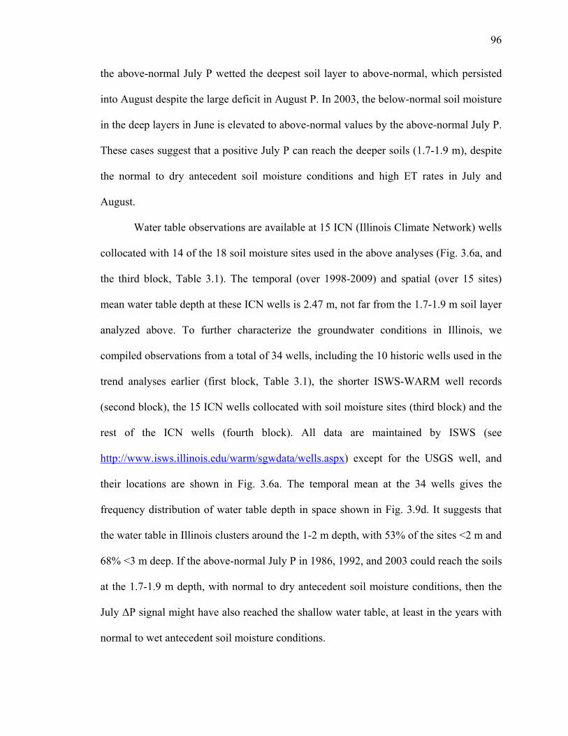
96
the above-normal July P wetted the deepest soil layer to above-normal, which persisted
into August despite the large deficit in August P. In 2003, the below-normal soil moisture
in the deep layers in June is elevated to above-normal values by the above-normal July P.
These cases suggest that a positive July P can reach the deeper soils (1.7-1.9 m), despite
the normal to dry antecedent soil moisture conditions and high ET rates in July and
August.
Water table observations are available at 15 ICN (Illinois Climate Network) wells
collocated with 14 of the 18 soil moisture sites used in the above analyses (Fig. 3.6a, and
the third block, Table 3.1). The temporal (over 1998-2009) and spatial (over 15 sites)
mean water table depth at these ICN wells is 2.47 m, not far from the 1.7-1.9 m soil layer
analyzed above. To further characterize the groundwater conditions in Illinois, we
compiled observations from a total of 34 wells, including the 10 historic wells used in the
trend analyses earlier (first block, Table 3.1), the shorter ISWS-WARM well records
(second block), the 15 ICN wells collocated with soil moisture sites (third block) and the
rest of the ICN wells (fourth block). All data are maintained by ISWS (see
http://www.isws.illinois.edu/warm/sgwdata/wells.aspx) except for the USGS well, and
their locations are shown in Fig. 3.6a. The temporal mean at the 34 wells gives the
frequency distribution of water table depth in space shown in Fig. 3.9d. It suggests that
the water table in Illinois clusters around the 1-2 m depth, with 53% of the sites <2 m and
68% <3 m deep. If the above-normal July P in 1986, 1992, and 2003 could reach the soils
at the 1.7-1.9 m depth, with normal to dry antecedent soil moisture conditions, then the
July ΔP signal might have also reached the shallow water table, at least in the years with
normal to wet antecedent soil moisture conditions.

97
3.4. Changes in ET
Lastly, we address the role of possible changes in ET. The increased groundwater
storage and streamflow in August-September could have been caused by the increased
July P, but it also could have been caused by reduced July ET, because it is P-ET, the net
soil water surplus, that reaches the water table. Since actual ET is not routinely and
historically observed, we infer changes in ET from changes in those variables that are
historically observed and indicative of ET, such as maximum air temperature, pan
evaporation, air relative humidity, and atmospheric vapor density deficit computed from
the latter two.
July mean daily maximum air temperature (Tmax) averaged over 104 station
records in the states of Illinois and Indiana (data from the NCDC) is plotted in Fig. 3.10a.
A notable cooling began in the mid 1950s and continued to the late 1970s. This is
consistent with the observed US (e.g., Liepert, 2002) and global-scale cooling due to
reduced solar radiation over the period of 1950-1980 (i.e., solar dimming, see recent
review by Wild, 2009) caused by changes in anthropogenic aerosols and their interaction
with changes in clouds. In the central US, the cooling has also been linked to large-scale
land-use changes such as converting forest to crops and particularly irrigation (e.g.,
Bonan, 2001; Govindasamy et al., 2001; Milly and Dunne, 2001; Baidya Roy et al., 2003;
Boucher et al., 2004; Feddema et al., 2005; Lobell et al., 2006, 2008; Adegoke et al.,
2007; Kueppers et al., 2007; Diffenbaugh, 2009). The mechanisms include the higher
albedo (reflecting more solar radiation) of croplands, increased latent vs. sensible heat
due to irrigation, and, indirectly, from increased cloud cover caused by higher ET, etc. A

98
recent global model simulation study (Puma and Cook, 2010) forced by observed sea
surface temperature and reconstructed global irrigation development history, shed much
light on the cause of the cooling by illustrating that cooling occurred in both the irrigation
and non-irrigation ensemble simulations, but more so in the ensemble with irrigation.
Although the causes might have been multiple, the cooling is certain.
The relevance of this cooling to the present study is that ET might have been
reduced since the 1950s, allowing deeper infiltration and water table recharge, without
additional precipitation. Records of observed pan evaporation, a direct indicator of
atmospheric ET demand, are available from six stations in Illinois and Indiana (from the
NCDC) dating back to at least the 1950s and continuing to the 1980s. Figures 3.10b-
3.10e plot the July total pan evaporation at these six sites, and Table 3.6 gives the site
information and the result of the Mann-Kendall trend analysis. There are no statistically
significant (at the 5% level) trends in any of these records, suggesting that the cooling
alone may not have caused a change in the atmospheric ET demand.
To supplement these few pan evaporation records, we assessed changes in ET
demand by computing the atmospheric vapor pressure deficit (VPD) from relative
humidity (RH) and air temperature (Ta) records. We found long-term observations of air
humidity at only three stations from the NCDC archive; unfortunately most of the long-
term records have a data gap (1948-1973) over our period of interest (1940-1980). The
VPD is computed as:
)100/1(* RHeVPD
a
a
T
Te
3.237
3.17exp611.0 Equation 1
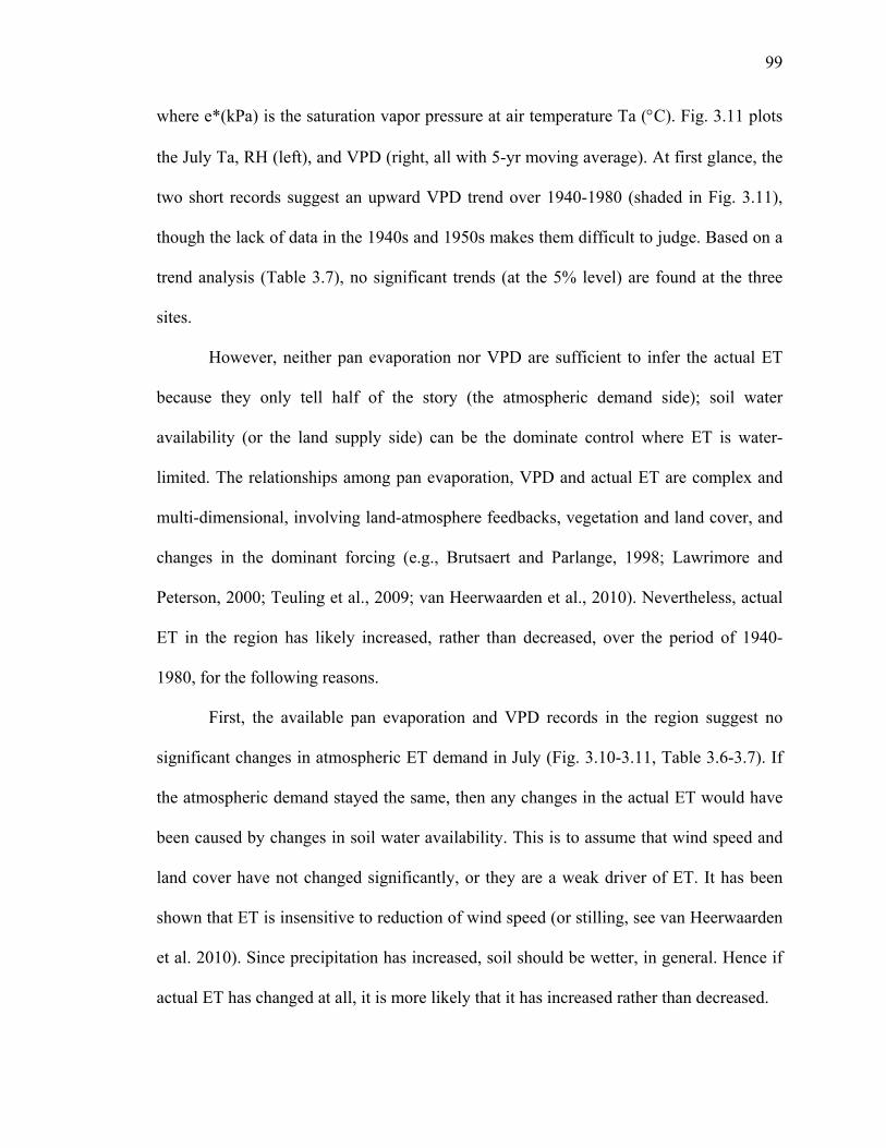
99
where e*(kPa) is the saturation vapor pressure at air temperature Ta (C). Fig. 3.11 plots
the July Ta, RH (left), and VPD (right, all with 5-yr moving average). At first glance, the
two short records suggest an upward VPD trend over 1940-1980 (shaded in Fig. 3.11),
though the lack of data in the 1940s and 1950s makes them difficult to judge. Based on a
trend analysis (Table 3.7), no significant trends (at the 5% level) are found at the three
sites.
However, neither pan evaporation nor VPD are sufficient to infer the actual ET
because they only tell half of the story (the atmospheric demand side); soil water
availability (or the land supply side) can be the dominate control where ET is water-
limited. The relationships among pan evaporation, VPD and actual ET are complex and
multi-dimensional, involving land-atmosphere feedbacks, vegetation and land cover, and
changes in the dominant forcing (e.g., Brutsaert and Parlange, 1998; Lawrimore and
Peterson, 2000; Teuling et al., 2009; van Heerwaarden et al., 2010). Nevertheless, actual
ET in the region has likely increased, rather than decreased, over the period of 1940-
1980, for the following reasons.
First, the available pan evaporation and VPD records in the region suggest no
significant changes in atmospheric ET demand in July (Fig. 3.10-3.11, Table 3.6-3.7). If
the atmospheric demand stayed the same, then any changes in the actual ET would have
been caused by changes in soil water availability. This is to assume that wind speed and
land cover have not changed significantly, or they are a weak driver of ET. It has been
shown that ET is insensitive to reduction of wind speed (or stilling, see van Heerwaarden
et al. 2010). Since precipitation has increased, soil should be wetter, in general. Hence if
actual ET has changed at all, it is more likely that it has increased rather than decreased.
100
Second, the idea that the actual ET in the region is driven by precipitation rather
than temperature is supported by a simple and elegant study of Teuling et al. (2009), who
conclude that changes in actual ET are governed by changes in its key driver (or limiting
factor) in a given region. That study shows that annual ET in the central US, inferred
from flux tower and multi-model syntheses, is far more responsive to changes in P than
changes in radiation. If this holds true for annual ET, it must hold true for warm-season
ET because the latter is more water-limited than all-season ET (Fig. 3.3a, P<ET in warm
season).
Third, the annual river basin water balance analyses in the same study (Teuling et
al., 2009) demonstrate that ET has increased over the period of solar dimming in the
upper Mississippi (including Illinois) and the Ohio River Basins. The upward trend in
annual ET is explained by the upward trend in annual P, which is partitioned into both
increased ET and increased streamflow, as has been shown in Milly and Dunne (2001)
and Qian et al. (2007) over the same region and period. Summer ET dominates annual
ET, and if annual ET has increased, then summer ET has likely increased as well.
Thus it is plausible that the increased July P caused both increased ET and
increased streamflow. This is corroborated by our earlier seasonal analysis, which
suggested that ET was likely to increase in response to the July ΔP signal, because ET
exceeds P and there is a net soil water deficit in the warm season. It is also consistent
with our earlier soil moisture analysis, which shows that present-day above-normal July P
could reach the deep soil in dry to normal antecedent soil moisture conditions despite
high ET demand. There is no evidence that ET has decreased due to cooling. We

101
conclude that the observed increase in late-summer groundwater storage and streamflow
in the Midwest is caused by the increased July precipitation.
4. Summary and Discussions
In this study, we set out to detect changes in land hydrology in response to the
increased July precipitation over the US Midwest attributed to High Plains’ irrigation in
an earlier study (DeAngelis et al., 2010). Seasonal analysis of hydrologic variables over
Illinois suggests that the seasonal cycle of P-ET is followed by the soil moisture cycle
one month later, which is followed by the water table and streamflow cycles another
month later, thus it is expected that the increased July P may be detected in August-
September groundwater and streamflow. We analyzed 30-year and longer time series of
water table depth at 10 wells in Illinois and streamflow at 46 gauges in the Illinois and
Ohio River basins. The Mann-Kendall test for trends indicates that groundwater storage
and streamflow have increased in August-September since the onset of irrigation in the
High Plains, and these trends were determined to be field significant. Examination of soil
moisture response to above-normal July P, in the post-irrigation era, suggests that the
increased July P due to High Plains’ irrigation can be sufficient to reach the shallow
water table at least in normal to wet years, hence providing a possible link between
increases in July P and groundwater storage and streamflow. The Mann-Kendall test for
trends in pan evaporation and atmospheric vapor pressure deficit, both indicators of
atmospheric ET demand, suggests that the ET demand has remained constant. The latter
points to the soil water availability as the driver in changes in ET and the possibility of

102
increased ET due to the increased P. Annual water balance study by Teuling et al. (2009)
gives further evidence of increased ET due to increased P. By ruling out the reduction in
ET as a cause, we conclude that the observed increase in groundwater storage and
streamflow in the Midwest is linked to the increased July precipitation attributed to High
Plains’ irrigation.
Historical changes in land use and land cover could also have affected the land
surface water budget in the study area. However, historic reconstructions (e.g.,
Ramankutty and Foley, 1999; Bonan, 2001) suggest that forest conversion to cropland
accelerated over 1850-1900 in the Midwestern states and slowed down significantly after
1900. In addition, conversion of forest to cropland has been shown to increase ET
(Bonan, 1999, 2001; Baidya Roy et al., 2003; Diffenbaugh, 2009), not to decrease ET.
Urban expansion can also affect water budget, but greater paved area is known to reduce
groundwater recharge and storage, not to increase it. Therefore land use change cannot
explain the observed increase in late summer groundwater storage and streamflow.
To place the observed increase in summer streamflow in the context of seasonal
dynamics, we plot in Fig. 3.12 the seasonal cycle difference at the 46 gauges between two
periods, 1940-1960 (early irrigation development) and 1960-1980 (late irrigation
development). Changes in August-September, the interest of this study, are rather small
compared to changes in March-April at many gauges, and hence its signal is buried in the
total annual flow which is often the focus of regional hydrologic change studies (e.g.,
Groisman et al., 2001; Zhang and Schiling, 2006; Qian et al., 2007; Kalra et al., 2008;
Raymond et al., 2008). We note that it is important to isolate the signals of change in
different seasons because they are likely caused by different mechanisms. Although the
103
signal of summer change is small, it is conceptually significant in that it may point to
human modification of the water cycle in the far-away High Plains region as a possible
source and cause.
Our results and their interpretations are limited by the available observations,
particularly the sparse and short records in water table depths, the lack of soil moisture
observations in the pre-irrigation era, and particularly the lack of actual ET
measurements. A regional climate-hydrology model simulation over irrigation
development era, similar to the approach in Puma and Cook (2010) but including fully
integrated hydrologic (including groundwater) and climatic interactions and feedbacks,
may help to disentangle the different causes of the observed hydrologic changes in the
study area.

104
Table 3.1. Information on groundwater observation wells used in this study (first block
shown in Fig. 3.9 and Table 3.2).
Site ID
Site Name
Lat.
Long.
Land Elevation
m
Well Depth
m
Year Begin
Year End
Obs. Frequency
Mean Water Table Depth
m
Wells with Early Data
USGS 41222008929
0301 USGS-1 41.37 89.47 212.75 8.84 1942 1990 10 days 3.34
ISWS-WARM W11
Cambridge 246.98 12.8 1961 2004 monthly 2.91
ISWS-WARM W21
Galena 222.69 7.62 1963 2007 monthly 6.50
ISWS-WARM W31
Mt. Morris 282.03 16.76 1960 2007 monthly 5.85
ISWS-WARM W41
Crystal Lake
273.04 5.49 1950 2007 monthly 1.57
ISWS-WARM W61
Barry 190.8 8.53 1956 2007 monthly 3.60
ISWS-WARM W91
Snicarte 148.29 12.8 1958 2007 monthly 11.29
ISWS-WARM W171
Sparta/Eden
156.06 8.23 1960 2007 monthly 2.27
ISWS-WARM W181
SWS No.2 128.35 24.38 1952 2004 monthly 4.52
ISWS-WARM W191
Dixon Springs
131.67 2.74 1955 2007 monthly 0.96
WTD mean 4.28 Other WARM
Wells
ISWS-WARM W53
Fermi 233.57 4.57 1988 2007 monthly 2.04
ISWS-WARM W72
Good Hope 233.17 9.14 1980 2007 monthly 2.44
ISWS-WARM W132
Greenfield 185.93 6.71 1965 2007 monthly 3.52
ISWS-WARM W143
Janesville 220.52 3.35 1969 2007 monthly 1.66
ISWS-WARM W153
St. Peter 182.27 4.57 1965 2007 monthly 0.94
ISWS-WARM W202
Harrisberg 116.13 3.35 1984 2007 monthly 1.39
ISWS-WARM W221
Boyleston 123.60 7.01 1984 2007 monthly 1.44
ISWS-WARM W1120
Bondville 213.91 6.40 1982 2007 monthly 1.27
WTD mean 1.84 ICN Wells at
SM Sites
ISWS-ICN W10
Bellville 38.52 89.88 133.00 6.10 2000 2010 Daily 1.65
ISWS-ICN W1 Bondville 40.05 88.37 213.00 6.10 2001 2010 Daily 1.44
ISWS-ICN W3 Brownstow
n 38.95 88.95 177.00 4.57 1997 2010 Daily 0.98
ISWS-ICN W11
Carbondale 37.70 89.23 137.00 7.62 2001 2010 Daily 1.53
ISWS-ICN W5 DeKalb 41.85 88.85 265.00 7.62 1997 2010 Daily 1.02
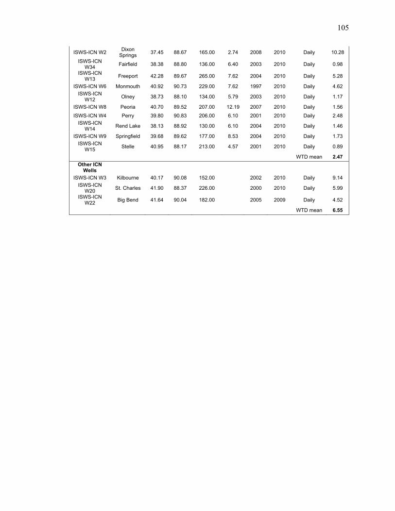
105
ISWS-ICN W2 Dixon
Springs 37.45 88.67 165.00 2.74 2008 2010 Daily 10.28
ISWS-ICN W34
Fairfield 38.38 88.80 136.00 6.40 2003 2010 Daily 0.98
ISWS-ICN W13
Freeport 42.28 89.67 265.00 7.62 2004 2010 Daily 5.28
ISWS-ICN W6 Monmouth 40.92 90.73 229.00 7.62 1997 2010 Daily 4.62
ISWS-ICN W12
Olney 38.73 88.10 134.00 5.79 2003 2010 Daily 1.17
ISWS-ICN W8 Peoria 40.70 89.52 207.00 12.19 2007 2010 Daily 1.56
ISWS-ICN W4 Perry 39.80 90.83 206.00 6.10 2001 2010 Daily 2.48
ISWS-ICN W14
Rend Lake 38.13 88.92 130.00 6.10 2004 2010 Daily 1.46
ISWS-ICN W9 Springfield 39.68 89.62 177.00 8.53 2004 2010 Daily 1.73
ISWS-ICN W15
Stelle 40.95 88.17 213.00 4.57 2001 2010 Daily 0.89
WTD mean 2.47 Other ICN
Wells
ISWS-ICN W3 Kilbourne 40.17 90.08 152.00 2002 2010 Daily 9.14
ISWS-ICN W20
St. Charles 41.90 88.37 226.00 2000 2010 Daily 5.99
ISWS-ICN W22
Big Bend 41.64 90.04 182.00 2005 2009 Daily 4.52
WTD mean 6.55
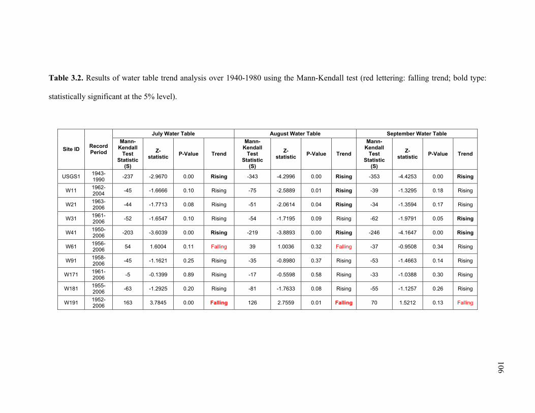
106
Table 3.2. Results of water table trend analysis over 1940-1980 using the Mann-Kendall test (red lettering: falling trend; bold type:
statistically significant at the 5% level).
July Water Table August Water Table September Water Table
Site ID Record Period
Mann-Kendall
Test Statistic
(S)
Z-statistic P-Value Trend
Mann-Kendall
Test Statistic
(S)
Z-statistic P-Value Trend
Mann-Kendall
Test Statistic
(S)
Z-statistic P-Value Trend
USGS1 1943-1990
-237 -2.9670 0.00 Rising -343 -4.2996 0.00 Rising -353 -4.4253 0.00 Rising
W11 1962-2004
-45 -1.6666 0.10 Rising -75 -2.5889 0.01 Rising -39 -1.3295 0.18 Rising
W21 1963-2006
-44 -1.7713 0.08 Rising -51 -2.0614 0.04 Rising -34 -1.3594 0.17 Rising
W31 1961-2006
-52 -1.6547 0.10 Rising -54 -1.7195 0.09 Rising -62 -1.9791 0.05 Rising
W41 1950-2006
-203 -3.6039 0.00 Rising -219 -3.8893 0.00 Rising -246 -4.1647 0.00 Rising
W61 1956-2006
54 1.6004 0.11 Falling 39 1.0036 0.32 Falling -37 -0.9508 0.34 Rising
W91 1958-2006
-45 -1.1621 0.25 Rising -35 -0.8980 0.37 Rising -53 -1.4663 0.14 Rising
W171 1961-2006
-5 -0.1399 0.89 Rising -17 -0.5598 0.58 Rising -33 -1.0388 0.30 Rising
W181 1955-2006
-63 -1.2925 0.20 Rising -81 -1.7633 0.08 Rising -55 -1.1257 0.26 Rising
W191 1952-2006
163 3.7845 0.00 Falling 126 2.7559 0.01 Falling 70 1.5212 0.13 Falling

107
Table 3.3. Information on the 46 stream gauges used in this study.
Gauge Sites USGS ID State Record
Period River Name Drainage Area (km2)
1 3345500 IL 1915-2009 EMBARRAS RIVER 3,926
2 3380500 IL 1909-2008 SKILLET FORK 1,202
3 3346000 IL 1941-2009 NORTH FORK EMBARRAS RIVER 824
4 3378000 IL 1941-2009 BONPAS CREEK 591
5 5419000 IL 1935-1977 APPLE RIVER 640
6 5420000 IL 1941-1977 PLUM RIVER 596
7 5435500 IL 1915-2009 PECATONICA RIVER 3,434
8 5440000 IL 1940-2009 KISHWAUKEE RIVER 2,846
9 5440500 IL 1940-1971 KILLBUCK CREEK 303
10 5444000 IL 1940-2009 ELKHORN CREEK 378
11 5448000 IL 1940-2008 MILL CREEK 162
12 5466500 IL 1935-1972 EDWARDS RIVER 1,153
13 5467000 IL 1935-2009 POPE CREEK 451
14 5469000 IL 1935-2009 HENDERSON CREEK 1,119
15 5469500 IL 1940-1971 SOUTH HENDERSON CREEK 215
16 5502040 IL 1940-1986 HADLEY CREEK 188
17 5513000 IL 1940-1986 BAY CREEK 383
18 5527500 IL 1915-2009 KANKAKEE RIVER 13,338
19 5529000 IL 1941-2009 DES PLAINES RIVER 932
20 5540500 IL 1941-2008 DU PAGE RIVER 839
21 5542000 IL 1940-2009 MAZON RIVER 1,178
22 5555500 IL 1932-1971 VERMILION RIVER 3,310
23 5556500 IL 1936-2009 BIG BUREAU CREEK 508
24 5583000 IL 1940-2009 SANGAMON RIVER 15,289
25 5592000 IL 1941-1970 KASKASKIA RIVER 2,730
26 5597000 IL 1908-1971 BIG MUDDY RIVER 2,056
27 3326500 IN 1924-2009 MISSISSINEWA RIVER 1,766
28 3340000 IN 1941-1971 SUGAR CREEK 1,735
29 3275000 IN 1929-2009 WHITEWATER RIVER 1,352
30 3328000 IN 1930-2009 EEL RIVER 1,080
31 3363500 IN 1931-2009 FLATROCK RIVER 785
32 3252500 KY 1938-2009 SOUTH FORK LICKING RIVER 1,608
33 3406500 KY 1936-2009 ROCKCASTLE RIVER 1,564
34 3314000 KY 1941-1971 DRAKES CREEK 1,238
35 3438000 KY 1940-2009 LITTLE RIVER 632
36 3217000 KY 1941-2009 TYGARTS CREEK 627
37 3299000 KY 1938-1992 ROLLING FORK 619
38 3219500 OH 1925-2010 SCIOTO RIVER 1,469
39 3230500 OH 1922-2009 BIG DARBY CREEK 1,383
40 3265000 OH 1917-2009 STILLWATER RIVER 1,303
41 3237500 OH 1926-2010 OHIO BRUSH CREEK 1,002
42 3232000 OH 1927-2009 PAINT CREEK 645

108
43 3238500 OH 1925-2009 WHITE OAK CREEK 565
44 3267000 OH 1926-2009 MAD RIVER 420
45 3434500 TN 1926-2009 HARPETH RIVER 1,764
46 3436000 TN 1939-1991 SULPHUR FORK RED RIVER 482
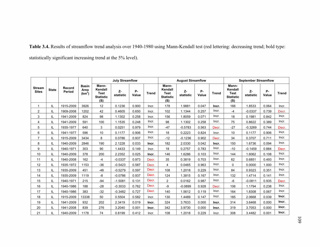
109
Table 3.4. Results of streamflow trend analysis over 1940-1980 using Mann-Kendall test (red lettering: decreasing trend; bold type:
statistically significant increasing trend at the 5% level).
July Streamflow August Streamflow September Streamflow
Stream Sites State Record
Period Basin Area (km2)
Mann-Kendall
Test Statistic
(S)
Z-statistic
P-Value Trend
Mann-Kendall
Test Statistic
(S)
Z-statistic
P-Value Trend
Mann-Kendall
Test Statistic
(S)
Z-statistic
P-Value Trend
1 IL 1915-2009 3926 12 0.1236 0.900 Incr. 178 1.9881 0.047 Incr. 166 1.8533 0.064 Incr.
2 IL 1909-2008 1202 42 0.4605 0.650 Incr. 102 1.1344 0.257 Incr. -4 -0.0337 0.739 Decr.
3 IL 1941-2009 824 98 1.1302 0.258 Incr. 156 1.8059 0.071 Incr. 18 0.1981 0.842 Incr. 4 IL 1941-2009 591 100 1.1535 0.248 Incr. 98 1.1302 0.258 Incr. 75 0.8622 0.389 Incr. 5 IL 1935-1977 640 3 0.0251 0.979 Incr. -47 -0.5783 0.563 Decr. -27 -0.3269 0.744 Decr.
6 IL 1941-1977 596 10 0.1177 0.906 Incr. 18 0.2223 0.824 Incr. 10 0.1177 0.906 Incr. 7 IL 1915-2009 3434 8 0.0786 0.937 Incr. -12 -0.1236 0.902 Decr. 34 0.3707 0.711 Incr. 8 IL 1940-2009 2846 190 2.1228 0.033 Incr. 182 2.0330 0.042 Incr. 150 1.6736 0.094 Incr. 9 IL 1940-1971 303 90 1.4433 0.149 Incr. 18 0.2757 0.783 Incr. -10 -0.1459 0.884 Decr.
10 IL 1940-2009 378 200 2.2352 0.025 Incr. 146 1.6286 0.103 Incr. 144 1.6062 0.108 Incr. 11 IL 1940-2008 162 -4 -0.0337 0.973 Decr. 35 0.3819 0.703 Incr. 62 0.6851 0.493 Incr. 12 IL 1935-1972 1153 -36 -0.5423 0.587 Decr. 4 0.0465 0.963 Incr. 0 0.0000 1.000 Incr. 13 IL 1935-2009 451 -48 -0.5279 0.597 Decr. 108 1.2018 0.229 Incr. 84 0.9323 0.351 Incr. 14 IL 1935-2009 1119 -8 -0.0786 0.937 Decr. 124 1.3815 0.167 Incr. 132 1.4714 0.141 Incr. 15 IL 1940-1971 215 -94 -1.5081 0.131 Decr. 2 0.0162 0.987 Incr. -6 -0.0811 0.935 Decr.
16 IL 1940-1986 188 -28 -0.3033 0.762 Decr. -9 -0.0899 0.928 Decr. 106 1.1794 0.238 Incr. 17 IL 1940-1986 383 -32 -0.3482 0.727 Decr. 140 1.5612 0.119 Incr. 164 1.8308 0.067 Incr. 18 IL 1915-2009 13338 50 0.5504 0.582 Incr. 130 1.4489 0.147 Incr. 185 2.0668 0.039 Incr. 19 IL 1941-2009 932 202 2.3419 0.019 Incr. 324 3.7633 0.000 Incr. 314 3.6468 0.000 Incr. 20 IL 1941-2008 839 276 3.2040 0.001 Incr. 342 3.9730 0.000 Incr. 319 3.7053 0.000 Incr. 21 IL 1940-2009 1178 74 0.8199 0.412 Incr. 108 1.2018 0.229 Incr. 308 3.4482 0.001 Incr.

110
22 IL 1932-1971 3310 24 0.3730 0.709 Incr. -50 -0.7946 0.427 Decr. -14 -0.2108 0.833 Decr.
23 IL 1936-2009 508 -38 -0.4156 0.677 Decr. 10 0.1011 0.920 Incr. 128 1.4265 0.154 Incr.
24 IL 1940-2009 15289 -8 -0.0786 0.937 Decr. 168 1.8757 0.061 Incr. 186 2.0779 0.038 Incr.
25 IL 1941-1970 2730 -55 -0.9634 0.335 Decr. 31 0.5352 0.593 Incr. 7 0.1070 0.915 Incr.
26 IL 1908-1971 2056 18 0.2757 0.782 Incr. 2 0.0162 0.987 Incr. -26 -0.4054 0.685 Decr.
27 IN 1924-2009 1766 52 0.5728 0.566 Incr. 158 1.7634 0.078 Incr. 196 2.1902 0.029 Incr.
28 IN 1941-1971 1735 59 0.9858 0.324 Incr. 43 0.7138 0.475 Incr. 37 0.6119 0.541 Incr. 29 IN 1929-2009 1352 120 1.3366 0.181 Incr. 132 1.4714 0.141 Incr. 132 1.4714 0.141 Incr. 30 IN 1930-2009 1080 8 0.0786 0.937 Incr. 89 0.9885 0.323 Incr. 144 1.6062 0.108 Incr. 31 IN 1931-2009 785 132 1.4714 0.141 Incr. 194 2.1678 0.030 Incr. 116 1.2917 0.196 Incr. 32 KY 1938-2009 1608 108 1.2018 0.229 Incr. 240 2.6844 0.007 Incr. 280 3.1337 0.002 Incr.
33 KY 1936-2009 1564 -42 -0.4605 0.645 Decr. 8 0.0786 0.937 Incr. 168 1.8757 0.061 Incr. 34 KY 1941-1971 1238 29 0.4759 0.634 Incr. 40 0.6630 0.507 Incr. 39 0.6459 0.518 Incr. 35 KY 1940-2009 632 46 0.5054 0.613 Incr. 85 0.9435 0.345 Incr. 119 1.3255 0.185 Incr. 36 KY 1941-2009 627 36 0.4078 0.683 Incr. 78 0.8971 0.370 Incr. 176 1.9656 0.049 Incr.
37 KY 1938-1992 619 -51 -0.5616 0.574 Decr. 144 1.6062 0.108 Incr. 178 1.9881 0.046 Incr.
38 OH 1925-2010 1469 42 0.4605 0.645 Incr. 55 0.6066 0.544 Incr. 148 1.6511 0.099 Incr.
39 OH 1922-2009 1383 90 0.9996 0.317 Incr. 173 1.9320 0.053 Incr. 240 2.6844 0.007 Incr.
40 OH 1917-2009 1303 66 0.7301 0.465 Incr. 58 0.6402 0.522 Incr. 122 1.3591 0.174 Incr. 41 OH 1926-2010 1002 110 1.2700 0.204 Incr. 276 3.2040 0.001 Incr. 168 1.9457 0.052 Incr. 42 OH 1927-2009 645 99 1.6656 0.095 Incr. 85 1.4277 0.153 Incr. 165 2.7874 0.005 Incr.
43 OH 1925-2009 565 148 1.6511 0.099 Incr. 268 2.9989 0.003 Incr. 138 1.5388 0.124 Incr. 44 OH 1926-2009 420 142 1.5837 0.113 Incr. 94 1.0446 0.296 Incr. 148 1.6511 0.099 Incr. 45 TN 1926-2009 1764 100 1.1120 0.266 Incr. 36 0.3931 0.694 Incr. 202 2.2576 0.024 Incr.
46 TN 1939-1991 482 132 1.4714 0.141 Incr. 170 1.8982 0.058 Incr. 109 1.2131 0.225 Incr.
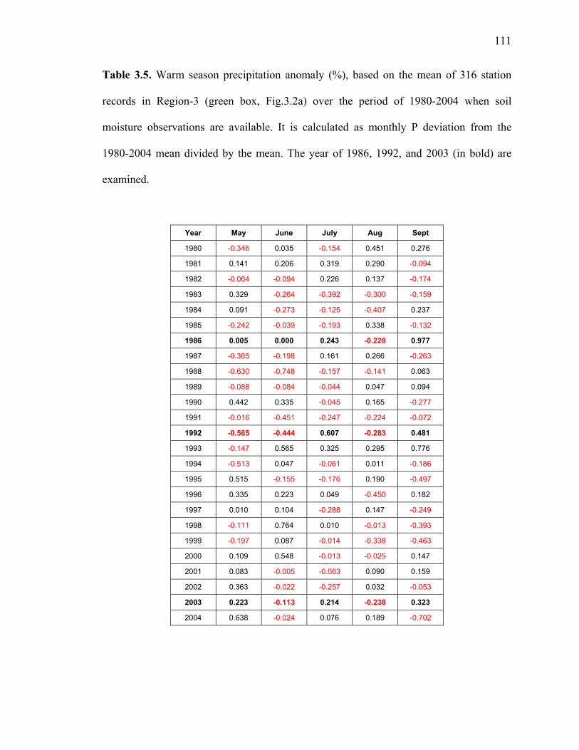
111
Table 3.5. Warm season precipitation anomaly (%), based on the mean of 316 station
records in Region-3 (green box, Fig.3.2a) over the period of 1980-2004 when soil
moisture observations are available. It is calculated as monthly P deviation from the
1980-2004 mean divided by the mean. The year of 1986, 1992, and 2003 (in bold) are
examined.
Year May June July Aug Sept
1980 -0.346 0.035 -0.154 0.451 0.276
1981 0.141 0.206 0.319 0.290 -0.094
1982 -0.064 -0.094 0.226 0.137 -0.174
1983 0.329 -0.264 -0.392 -0.300 -0.159
1984 0.091 -0.273 -0.125 -0.407 0.237
1985 -0.242 -0.039 -0.193 0.338 -0.132
1986 0.005 0.000 0.243 -0.228 0.977
1987 -0.365 -0.198 0.161 0.266 -0.263
1988 -0.630 -0.748 -0.157 -0.141 0.063
1989 -0.088 -0.084 -0.044 0.047 0.094
1990 0.442 0.335 -0.045 0.165 -0.277
1991 -0.016 -0.451 -0.247 -0.224 -0.072
1992 -0.565 -0.444 0.607 -0.283 0.481
1993 -0.147 0.565 0.325 0.295 0.776
1994 -0.513 0.047 -0.061 0.011 -0.186
1995 0.515 -0.155 -0.176 0.190 -0.497
1996 0.335 0.223 0.049 -0.450 0.182
1997 0.010 0.104 -0.288 0.147 -0.249
1998 -0.111 0.764 0.010 -0.013 -0.393
1999 -0.197 0.087 -0.014 -0.338 -0.463
2000 0.109 0.548 -0.013 -0.025 0.147
2001 0.083 -0.005 -0.063 0.090 0.159
2002 0.363 -0.022 -0.257 0.032 -0.053
2003 0.223 -0.113 0.214 -0.238 0.323
2004 0.638 -0.024 0.076 0.189 -0.702

112
Table 3.6. July pan evaporation site information and Mann-Kendall test results for trends over 1940-1980. No significant
trends (at the 5% level) are found at the six sites.
July Pan Evaporation Coop ID Site Name State Latitude Longitude Elevation
m Period Mean mm Mann-Kendall
Test Statistic (S) Z-
statistic P-
Value Trend
118179 Springfield Capital AP IL 39.83 -89.68 181 1948-1990 227 36 0.6920 0.49 Increasing
122309 Dubois S in Forage FM IN 38.45 -86.70 210 1957-1999 180 13 0.2980 0.77 Increasing
122738 Evansville Regional AP IN 38.03 -87.52 122 1948-1987 205 58 0.8836 0.38 Increasing
126506 Oaklandon Geist RSVR IN 39.90 -85.98 242 1937-1998 159 -119 -1.3755 0.17 Decreasing
128999 Valparaiso WTR WKS IN 41.50 -87.03 244 1948-1999 150 -62 -0.9457 0.34 Decreasing
129430 West Lafayette 6 NW IN 40.47 -86.98 218 1957-1999 192 33 0.7947 0.43 Increasing
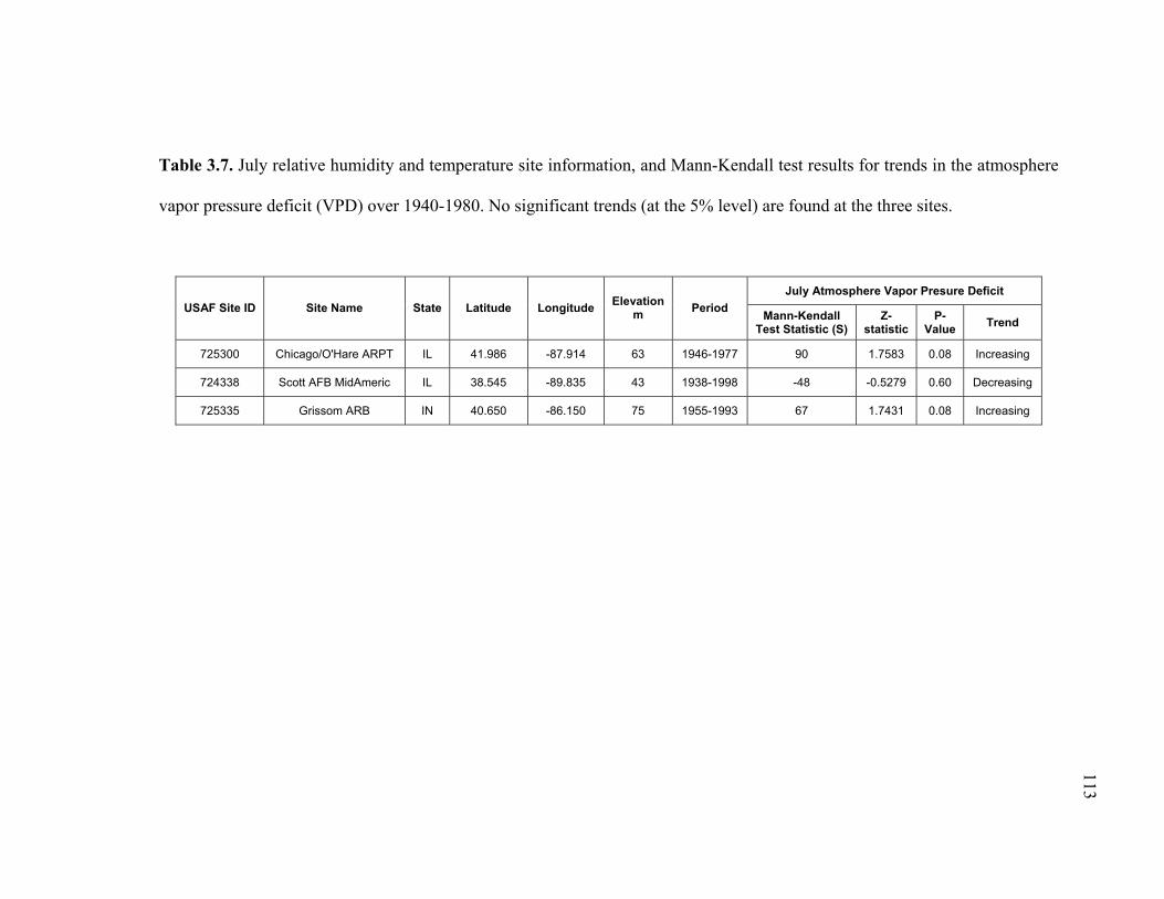
113
Table 3.7. July relative humidity and temperature site information, and Mann-Kendall test results for trends in the atmosphere
vapor pressure deficit (VPD) over 1940-1980. No significant trends (at the 5% level) are found at the three sites.
July Atmosphere Vapor Presure Deficit USAF Site ID Site Name State Latitude Longitude Elevation
m Period Mann-Kendall Test Statistic (S)
Z-statistic
P-Value Trend
725300 Chicago/O'Hare ARPT IL 41.986 -87.914 63 1946-1977 90 1.7583 0.08 Increasing
724338 Scott AFB MidAmeric IL 38.545 -89.835 43 1938-1998 -48 -0.5279 0.60 Decreasing
725335 Grissom ARB IN 40.650 -86.150 75 1955-1993 67 1.7431 0.08 Increasing
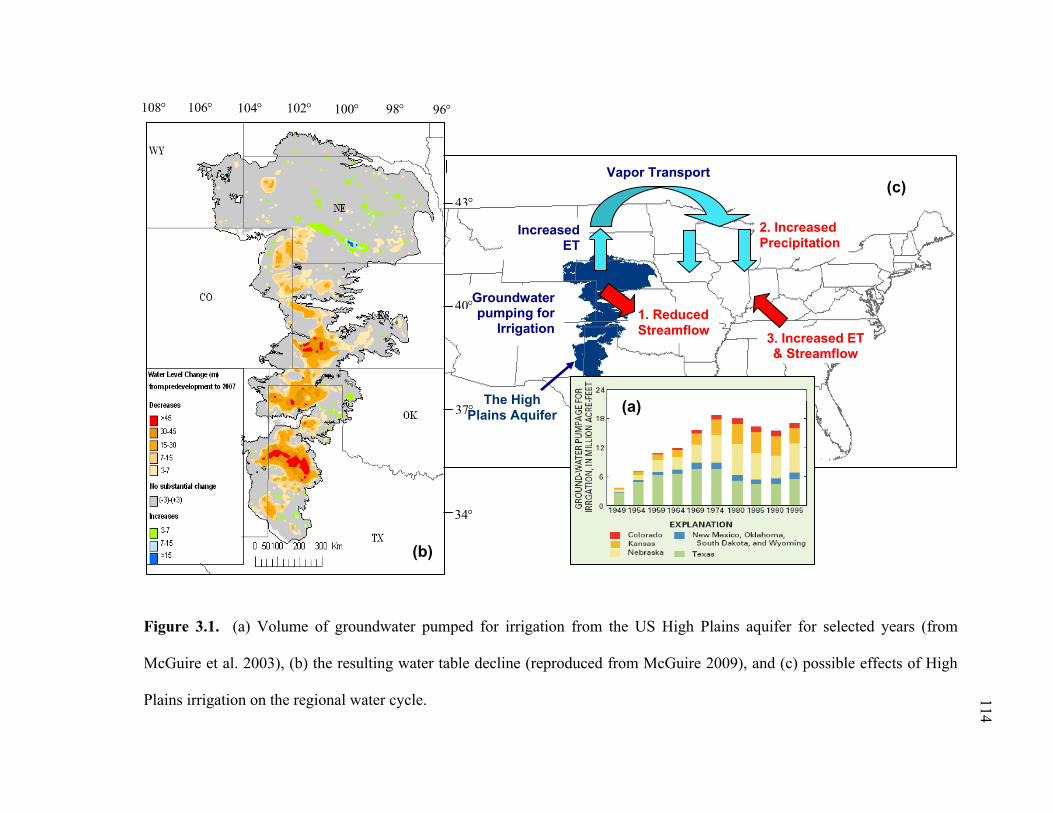
114
Figure 3.1. (a) Volume of groundwater pumped for irrigation from the US High Plains aquifer for selected years (from
McGuire et al. 2003), (b) the resulting water table decline (reproduced from McGuire 2009), and (c) possible effects of High
Plains irrigation on the regional water cycle.
(c)
1. Reduced Streamflow 3. Increased ET
& Streamflow
Groundwater pumping for
Irrigation
2. Increased Precipitation
The High Plains Aquifer
Vapor Transport
Increased ET
40
37
34
43
(a)
104 102 106 108 100 98 96
(b)

115
Figure 3.2. (a) Spatial pattern of July precipitation change (%) between periods of
(1900-1950) and (1950-2000), with mean July 850 mb wind fields (m/s) over 1979-2001,
obtained from North America Regional Reanalysis (for details see DeAngelis et al.,
2010), (b) time series of July precipitation (mm) averaged over 316 station records within
Region 3- the area of focus of this study (green box in a), shown as 5-year moving
average, and with mean (blue) of the first and second half of the century (84 and 102 mm,
respectively, tested statistically significant in DeAngelis et al. (2010)).
140
120
100
80
60
40
Reg
-3 J
uly
P
200019801960194019201900
Region 1 Region 3 Region 2
(a)
(b)

116
Figure 3.3. Seasonal Cycle, (a) in precipitation (P), evapotranspiration (ET), land surface
surplus (P-ET), streamflow (Qr), and (b) in SM and WTD (data from Eltahir and Yeh,
1999).
150
100
50
0
P, E
T, P
-ET
, Str
eam
flow
(m
m)
121110987654321Month
Ppt ET Qr P_ET
38
36
34
32
30
Top
2m
Soi
l Moi
stur
e (%
)
121110987654321Month
-4.0
-3.8
-3.6
-3.4
-3.2
-3.0
-2.8
-2.6
Water T
able Depth (m
)
SM WTD
20% increase
(b)
(a)
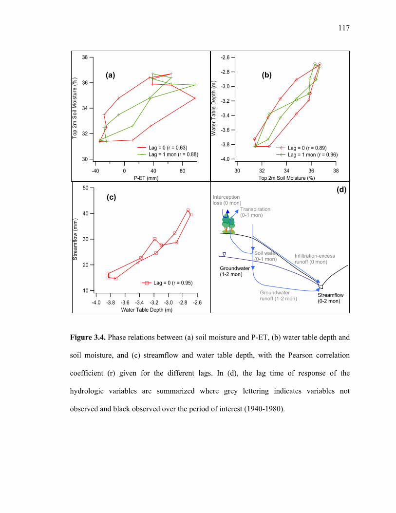
117
Figure 3.4. Phase relations between (a) soil moisture and P-ET, (b) water table depth and
soil moisture, and (c) streamflow and water table depth, with the Pearson correlation
coefficient (r) given for the different lags. In (d), the lag time of response of the
hydrologic variables are summarized where grey lettering indicates variables not
observed and black observed over the period of interest (1940-1980).
(a) (b)
(c) (d)
Infiltration-excess runoff (0 mon)
Soil water (0-1 mon)
Groundwater (1-2 mon)
Groundwater runoff (1-2 mon)
Transpiration (0-1 mon)
38
36
34
32
30
Top
2m
Soi
l Moi
stur
e (%
)
80400-40P-ET (mm)
Lag = 0 (r = 0.63) Lag = 1 mon (r = 0.88)
-4.0
-3.8
-3.6
-3.4
-3.2
-3.0
-2.8
-2.6
Wat
er T
able
Dep
th (
m)
3836343230Top 2m Soil Moisture (%)
Lag = 0 (r = 0.89) Lag = 1 mon (r = 0.96)
50
40
30
20
10
Str
eam
flow
(m
m)
-4.0 -3.8 -3.6 -3.4 -3.2 -3.0 -2.8 -2.6Water Table Depth (m)
Lag = 0 (r = 0.95)
Streamflow (0-2 mon)
Interception loss (0 mon)

118
May
June
July
Aug
Sept
Figure 3.5. Region-3 mean monthly rainfall (5-yr moving average) for May, June, July,
August and September based on 316 station records, with the irrigation development
period (1940-1980) shown on the top in grey shade.
150
120
90
60Reg
3 S
ep P
reci
p (m
m)
20001990198019701960195019401930192019101900Year
150
120
90
60Reg
3 A
ug P
reci
p (m
m)
20001990198019701960195019401930192019101900
150
120
90
60Reg
3 Ju
l Pre
cip
(mm
)
20001990198019701960195019401930192019101900
150
120
90
60Reg
3 Ju
n P
reci
p (m
m)
20001990198019701960195019401930192019101900
150
120
90
60Reg
3 M
ay P
reci
p (m
m)
20001990198019701960195019401930192019101900
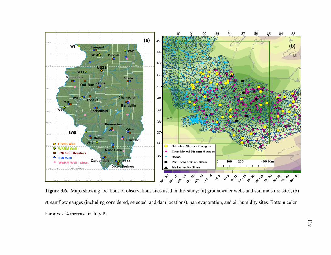
119
-35 -
-30
-30 -
-25
-25-
-20
-20 -
-15
-15-
-10
-10 -
-5
-5- 0 0 - 5
5 - 10
10 -
1515
- 20
20 -
2525
- 30
30 -
3535
- 40
40 -
45
Figure 3.6. Maps showing locations of observations sites used in this study: (a) groundwater wells and soil moisture sites, (b)
streamflow gauges (including considered, selected, and dam locations), pan evaporation, and air humidity sites. Bottom color
bar gives % increase in July P.
(a)
42 0
41 5
41 0
40 5
40 0
39 5
39 0
38 5
38 0
37 0
42 5
91 0 90 5 90 0 89 5 88 5 88 0 87 591 5
Freeport
DeKalb
StellePeoria
Monmouth
Perr
Springfield
Olne
Fairfield
Brownstown
Rend Lake
Bellvill
Carbondale W191
Oak Run
ChampaignTopeka
ICN Soil MoistureWARM Well -USGS Well W17
SWS
W61
W9
W11
W31
W2W41
USGS
Dixon Springs
Bondville
ICN WellWARM Well - short
(b)
37
36
45
92 85
42
38
41
39
44
43
86 8788 8990 91
35
84 83
40
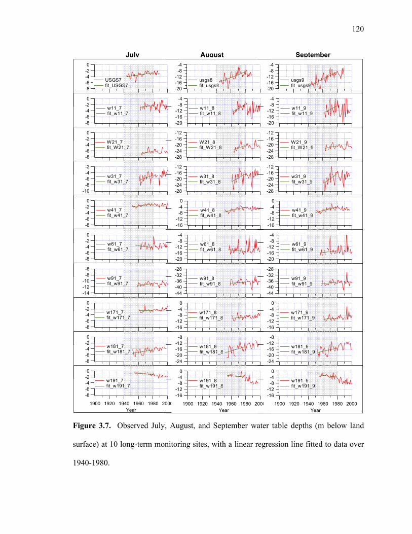
120
Figure 3.7. Observed July, August, and September water table depths (m below land
surface) at 10 long-term monitoring sites, with a linear regression line fitted to data over
1940-1980.
-8-6-4-20
200019801960194019201900
USGS7 fit_USGS7
-8-6-4-20
200019801960194019201900
w11_7 fit_w11_7
-8-6-4-20
200019801960194019201900
W21_7 fit_W21_7
-10-8-6-4-2
200019801960194019201900
w31_7 fit_w31_7
-8-6-4-20
200019801960194019201900
w41_7 fit_w41_7
-8-6-4-20
200019801960194019201900
w61_7 fit_w61_7
-14-12-10
-8-6
200019801960194019201900
w91_7 fit_w91_7
-8-6-4-20
200019801960194019201900
w171_7 fit_w171_7
-8-6-4-20
200019801960194019201900
w181_7 fit_w181_7
-8-6-4-20
200019801960194019201900Year
w191_7 fit_w191_7
-20-16-12
-8-4
200019801960194019201900
usgs8 fit_usgs8
-20-16-12
-8-4
200019801960194019201900
w11_8 fit_w11_8
-28-24-20-16-12
200019801960194019201900
W21_8 fit_W21_8
-28-24-20-16-12
200019801960194019201900
w31_8 fit_w31_8
-16-12
-8-40
200019801960194019201900
w41_8 fit_w41_8
-20-16-12
-8-4
200019801960194019201900
w61_8 fit_w61_8
-44-40-36-32-28
200019801960194019201900
w91_8 fit_w91_8
-16-12
-8-40
200019801960194019201900
w171_8 fit_w171_8
-24-20-16-12
-8
200019801960194019201900
w181_8 fit_w181_8
-16-12
-8-40
200019801960194019201900Year
w191_8 fit_w191_8
-20-16-12
-8-4
200019801960194019201900
usgs9 fit_usgs9
-20-16-12
-8-4
200019801960194019201900
w11_9 fit_w11_9
-28-24-20-16-12
200019801960194019201900
W21_9 fit_W21_9
-28-24-20-16-12
200019801960194019201900
w31_9 fit_w31_9
-16-12
-8-40
200019801960194019201900
w41_9 fit_w41_9
-20-16-12
-8-4
200019801960194019201900
w61_9 fit_w61_9
-44-40-36-32-28
200019801960194019201900
w91_9 fit_w91_9
-16-12
-8-40
200019801960194019201900
w171_9 fit_w171_9
-24-20-16-12
-8
200019801960194019201900
w181_9 fit_w181_9
-16-12
-8-40
200019801960194019201900Year
w191_9 fit_w191_9
July August September
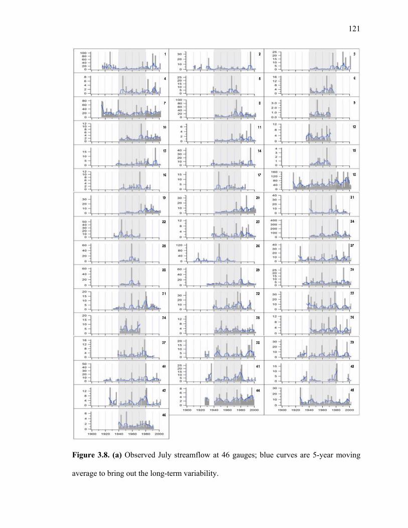
121
Figure 3.8. (a) Observed July streamflow at 46 gauges; blue curves are 5-year moving
average to bring out the long-term variability.

122
Figure 3.8. (b) Observed August streamflow at 46 gauges; blue curves are 5-year moving
average to bring out the long-term variability.
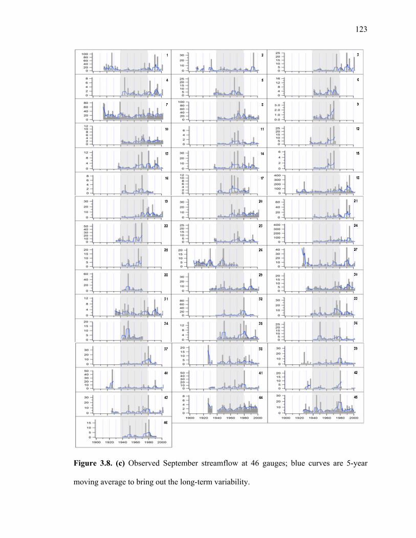
123
Figure 3.8. (c) Observed September streamflow at 46 gauges; blue curves are 5-year
moving average to bring out the long-term variability.
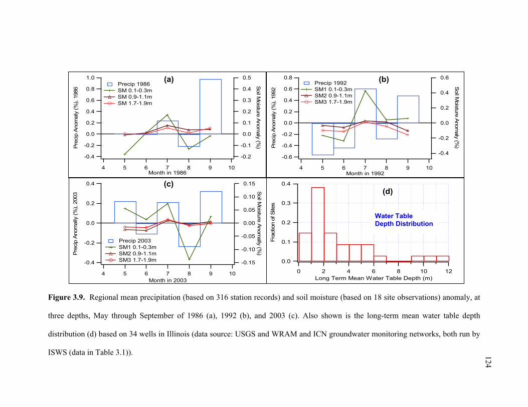
124
Figure 3.9. Regional mean precipitation (based on 316 station records) and soil moisture (based on 18 site observations) anomaly, at
three depths, May through September of 1986 (a), 1992 (b), and 2003 (c). Also shown is the long-term mean water table depth
distribution (d) based on 34 wells in Illinois (data source: USGS and WRAM and ICN groundwater monitoring networks, both run by
ISWS (data in Table 3.1)).
1.0
0.8
0.6
0.4
0.2
0.0
-0.2
-0.4
Pre
cip A
nom
aly
(%
), 1
986
10987654Month in 1986
0.5
0.4
0.3
0.2
0.1
0.0
-0.1
-0.2
Soil M
oistu
re A
nom
aly (%
)
Precip 1986 SM 0.1-0.3m SM 0.9-1.1m SM 1.7-1.9m
(a)
-0.4
-0.2
0.0
0.2
0.4
Pre
cip A
nom
ally
(%
), 2
003
10987654Month in 2003
-0.15
-0.10
-0.05
0.00
0.05
0.10
0.15
Soil M
oistu
re A
nom
ally (%
)
Precip 2003 SM1 0.1-0.3m SM2 0.9-1.1m SM3 1.7-1.9m
0.4
0.3
0.2
0.1
0.0
Fra
ctio
n o
f Site
s121086420
Long Term Mean Water Table Depth (m)
(d)
Water Table Depth Distribution
0.8
0.6
0.4
0.2
0.0
-0.2
-0.4
-0.6
Pre
cip
Anom
aly
(%
), 1
992
10987654Month in 1992
0.6
0.4
0.2
0.0
-0.2
-0.4
Soil M
oisture
Anom
aly (%)
Precip 1992 SM1 0.1-0.3m SM2 0.9-1.1m SM3 1.7-1.9m
(b)
(c)
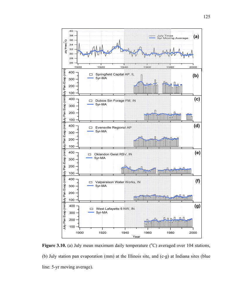
125
Figure 3.10. (a) July mean maximum daily temperature (oC) averaged over 104 stations,
(b) July station pan evaporation (mm) at the Illinois site, and (c-g) at Indiana sites (blue
line: 5-yr moving average).
40
38
36
34
32
30
28
26Ju
ly Tmax
(o
C)
200019801960194019201900Year
July Tmax 5yr Moving Average (a)
400
300
200
100
July
Pan
Eva
p (m
m)
200019801960194019201900
Springfield Capital AP, IL 5yr-MA
400
300
200
100
July
Pan
Eva
p (m
m)
200019801960194019201900
Dubios Sin Forage FM, IN 5yr-MA
400
300
200
100
July
Pan
Eva
p (m
m)
200019801960194019201900
Evensville Regional AP 5yr-MA
400
300
200
100
July
Pan
Eva
p (m
m)
200019801960194019201900Year
Oklandon Geist RSV, IN 5yr-MA
400
300
200
100
July
Pan
Eva
p (m
m)
200019801960194019201900
Valparaison Water Works, IN 5yr-MA
400
300
200
100
July
Pan
Eva
p (m
m)
200019801960194019201900Year
West Lafayette 6 NW, IN 5yr-MA
(b)
(c)
(d)
(e)
(f)
(g)
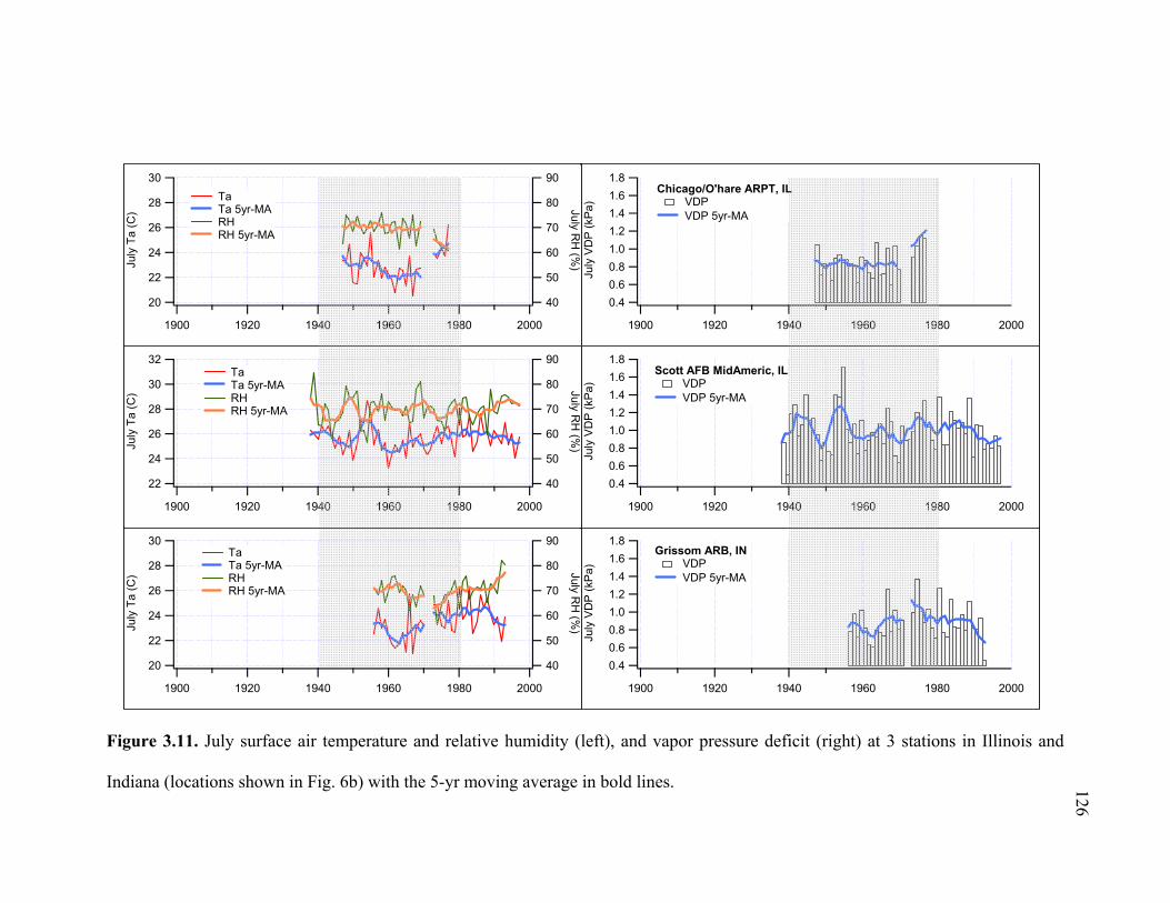
126
Figure 3.11. July surface air temperature and relative humidity (left), and vapor pressure deficit (right) at 3 stations in Illinois and
Indiana (locations shown in Fig. 6b) with the 5-yr moving average in bold lines.
1.8
1.6
1.4
1.2
1.0
0.8
0.6
0.4
July
VD
P (
kPa)
200019801960194019201900
Grissom ARB, IN VDP VDP 5yr-MA
30
28
26
24
22
20
July
Ta
(C)
200019801960194019201900
90
80
70
60
50
40
July RH
(%)
Ta Ta 5yr-MA RH RH 5yr-MA
1.8
1.6
1.4
1.2
1.0
0.8
0.6
0.4
July
VD
P (
kPa)
200019801960194019201900
Scott AFB MidAmeric, IL VDP VDP 5yr-MA
32
30
28
26
24
22
July
Ta
(C)
200019801960194019201900
90
80
70
60
50
40
July RH
(%)
Ta Ta 5yr-MA RH RH 5yr-MA
1.8
1.6
1.4
1.2
1.0
0.8
0.6
0.4
July
VD
P (
kPa)
200019801960194019201900
Chicago/O'hare ARPT, IL VDP VDP 5yr-MA
30
28
26
24
22
20
July
Ta
(C)
200019801960194019201900
90
80
70
60
50
40
July RH
(%)
Ta Ta 5yr-MA RH RH 5yr-MA
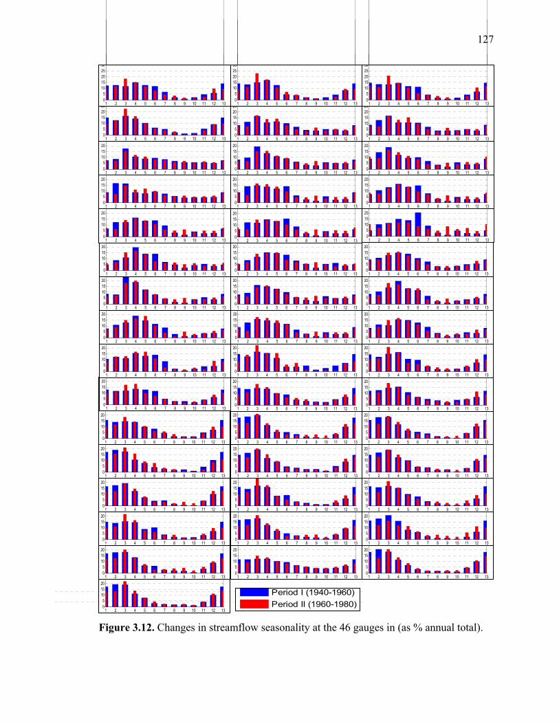
127
Figure 3.12. Changes in streamflow seasonality at the 46 gauges in (as % annual total).
1 2 3 4 5 6 7 8 9 10 11 12 1305
101520253035404550
1 2 3 4 5 6 7 8 9 10 11 12 1305
101520253035404550
1 2 3 4 5 6 7 8 9 10 11 12 13
05
101520253035404550
1 2 3 4 5 6 7 8 9 10 11 12 13
05
101520253035404550
1 2 3 4 5 6 7 8 9 10 11 12 1305
101520253035404550
1 2 3 4 5 6 7 8 9 10 11 12 13
05
101520253035404550
1 2 3 4 5 6 7 8 9 10 11 12 13
05
101520253035404550
1 2 3 4 5 6 7 8 9 10 11 12 1305
101520253035404550
1 2 3 4 5 6 7 8 9 10 11 12 13
05
101520253035404550
1 2 3 4 5 6 7 8 9 10 11 12 13
05
101520253035404550
1 2 3 4 5 6 7 8 9 10 11 12 1305
101520253035404550
1 2 3 4 5 6 7 8 9 10 11 12 13
05
101520253035404550
1 2 3 4 5 6 7 8 9 10 11 12 13
05
101520253035404550
1 2 3 4 5 6 7 8 9 10 11 12 1305
101520253035404550
1 2 3 4 5 6 7 8 9 10 11 12 13
05
101520253035404550
1 2 3 4 5 6 7 8 9 10 11 12 13
05
101520253035404550
1 2 3 4 5 6 7 8 9 10 11 12 1305
101520253035404550
1 2 3 4 5 6 7 8 9 10 11 12 13
05
101520253035404550
1 2 3 4 5 6 7 8 9 10 11 12 13
05
101520253035404550
1 2 3 4 5 6 7 8 9 10 11 12 1305
101520253035404550
1 2 3 4 5 6 7 8 9 10 11 12 13
05
101520253035404550
1 2 3 4 5 6 7 8 9 10 11 12 13
05
101520253035404550
1 2 3 4 5 6 7 8 9 10 11 12 1305
101520253035404550
1 2 3 4 5 6 7 8 9 10 11 12 13
05
101520253035404550
1 2 3 4 5 6 7 8 9 10 11 12 13
05
101520253035404550
1 2 3 4 5 6 7 8 9 10 11 12 130
5101520253035404550
1 2 3 4 5 6 7 8 9 10 11 12 13
0
5101520253035404550
1 2 3 4 5 6 7 8 9 10 11 12 13
0
5101520253035404550
1 2 3 4 5 6 7 8 9 10 11 12 1305
101520253035404550
1 2 3 4 5 6 7 8 9 10 11 12 13
05
101520253035404550
1 2 3 4 5 6 7 8 9 10 11 12 13
05
101520253035404550
1 2 3 4 5 6 7 8 9 10 11 12 1305
101520253035404550
1 2 3 4 5 6 7 8 9 10 11 12 13
05
101520253035404550
1 2 3 4 5 6 7 8 9 10 11 12 13
05
101520253035404550
1 2 3 4 5 6 7 8 9 10 11 12 1305
101520253035404550
1 2 3 4 5 6 7 8 9 10 11 12 13
05
101520253035404550
1 2 3 4 5 6 7 8 9 10 11 12 13
05
101520253035404550
1 2 3 4 5 6 7 8 9 10 11 12 1305
101520253035404550
1 2 3 4 5 6 7 8 9 10 11 12 13
05
101520253035404550
1 2 3 4 5 6 7 8 9 10 11 12 13
05
101520253035404550
1 2 3 4 5 6 7 8 9 10 11 12 1305
101520253035404550
1 2 3 4 5 6 7 8 9 10 11 12 13
05
101520253035404550
1 2 3 4 5 6 7 8 9 10 11 12 13
05
101520253035404550
1 2 3 4 5 6 7 8 9 10 11 12 1305
1015202530
1 2 3 4 5 6 7 8 9 10 11 12 13
05
1015202530
1 2 3 4 5 6 7 8 9 10 11 12 13
05
1015202530
Period I (1940-1960)
Period II (1960-1980)

128
Chapter 4
Summary and Future Work
1. Summary
In this dissertation, a comprehensive study on the impacts of large-scale irrigation
in the US High Plains on regional hydrology and climate is presented to elucidate the
influence of anthropogenic perturbations on the hydrological cycle. With an emphasis on
large-scale hydro-climatic linkages and feedbacks, it is hypothesized that the regional
irrigation development in the High Plains has had three potential impacts: 1) streamflow
depletion in the High Plains due to excessive irrigational pumping, particularly in areas
where groundwater is the main source of streamflow, 2) downwind precipitation increase
due to irrigation-enhanced evapotranspiration (ET) and vapor export during the warm-
season, and 3) subsequent increases in downwind groundwater storage and streamflow
due to increased warm-season precipitation.
The first hypothesis was tested in Chapter 2 by focusing on the detection of
changes in annual and seasonal streamflow regimes in response to the development of
extensive irrigational pumping in the High Plains since the 1950’s. After compiling all
available records, the degree of hydraulic connection between groundwater and
streamflow throughout the High Plains was systematically examined with special
attention to the hydro-climatic gradients across the region. Phase relationships between
streamflow, groundwater levels, and precipitation time series revealed that the
129
groundwater-streamflow connection gradually decreases from the Northern to the
Southern High Plains. The trend results in annual and dry-season (mean of July and
August) streamflow are in agreement with this regional pattern indicating that streamflow
depletion is more pronounced in the north and less apparent in the south. The step change
results show that the observed depletions in streamflow correlate well with significant
declines in groundwater levels. The insignificant changes in precipitation over the region
further suggest that streamflow depletion is closely-related to the decreases in water table
levels. Additionally, the annual number of low-flow days was found to be increasing in
the highly-irrigated watersheds on Northern High Plains, suggesting that groundwater
pumping is the main cause. Consequently, excessive irrigational pumping in the High
Plains has likely resulted in streamflow depletion more significantly in the northern part
where groundwater sustains the local streams, and less significantly towards the south
where streams are dependent mainly on local precipitation. The results of Chapter 2
provide a regional analysis of the effect of groundwater pumping on High Plains’
streamflow using a consistent methodology and filling the large spatial gaps between the
previously-studied areas.
The second hypothesis was tested in DeAngelis et al. (2010) by analyzing an
extensive amount of century-long precipitation records over and downwind of the High
Plains with an emphasis on the irrigation impacts on regional climate. Statistical test
results indicated a significant increase in precipitation (~20%) over the Midwest during
the peak irrigation month, July. The timing (around 1950) and spatial pattern of observed
precipitation increase coincided with the onset of intensive irrigation development in the
High Plains (1940-1980) and the pathway of Great Plains Low Level Jet. Moreover, a
130
Lagrangian vapor tracking analysis showed that the additional moisture from the High
Plains contributes to downwind precipitation and the contribution increases when ET is
higher. This further supports the physical link between the High Plains’ irrigation and
observed increases in July precipitation over the Midwest. Besides, the possible role of
macro-scale atmospheric circulation changes in the observed precipitation increases was
investigated and no evidence was found.
Finally, the third hypothesis was tested in Chapter 3 by investigating changes in
land surface hydrologic variables that may be attributable to the observed increase in July
precipitation during the second half of the century. Concentrating on areas where July
precipitation increased by 10-30%, available observations of soil moisture, ET,
groundwater, and streamflow in Illinois and Indiana are analyzed. Seasonal analyses of
regional land hydrology suggested that response of the water table and streamflow to
increased July precipitation could lag by 1-2 months. Accordingly, the Mann-Kendall test
for trends indicated increases in groundwater storage and streamflow during August and
September that were field-significant and coincident with the timing of irrigation
expansion. Furthermore, it is found that the soil moisture allows the above-normal
precipitation in July to reach the shallow water table in normal to wet years. This
strengthens the possible link between irrigation-enhanced July precipitation and increased
groundwater storage and streamflow in the region. Also, indicators of atmospheric ET
demand did not reveal any significant changes in July ET during the post-irrigation
period, suggesting that changes in July ET should be associated with the water
availability in the region. As a result of surplus July rainfall, the actual ET is likely to
have increased rather than decreased, hence, the role of a possible ET reduction in the
131
observed increases in August-September groundwater storage and streamflow could be
eliminated, leaving the increased July precipitation as the main cause.
The overall results of this research demonstrate that large-scale irrigation in the
High Plains has significantly altered the regional hydrology and climate during the
second half of the last century. This work has important implications in regard to the
extent of the impacts of human activities on the hydrologic cycle. It has been shown
herein that part of the decreased water in surface and subsurface storages in the west of
the Mississippi River ends up in the east part of it through an anthropogenically-modified
water cycle. This underlines the fact that human activities alter the hydrological cycle not
only at local but also at regional scales. Also, attribution of observed hydrologic changes
to correct causes is extremely important for future assessment of natural and
anthropogenic-induced climate changes.
2. Future Work
The contributions of this study to the understanding of direct human impacts on
the regional hydrological cycle are noteworthy; nevertheless there remain some caveats
that require further investigation albeit some are beyond the scope of this work:
1) Results presented in this research are evaluated based only on in situ
observational data which often has limited availability. The observed
changes in the study area can be better understood with the use of a
fully-coupled land-atmosphere model which includes groundwater
dynamics (e.g. York et al., 2002; Yeh and Eltahir, 2005; Fan et al.,

132
2007; Niu et al. 2007; Kollet and Maxwell, 2008; Jiang et al., 2009)
and incorporates both satellite-derived and in situ observations.
2) It has been speculated that timing of snowmelt in the western US,
which is the main source of regional groundwater in the High Plains,
has shifted earlier due to recent increases in land surface temperatures
(Dettinger and Cayan, 1995; Hamlet et al., 2005; Regonda et al., 2005;
Stewart et al. 2005). This could also have affected water table levels in
the region besides pumping, thus needs to be investigated in a future
study. An important question might be; what is the impact of changing
patterns in the western US snowmelt on High Plains groundwater and
streamflow regimes? The answer to this question might partly explain
the reason of less significant decreasing trends observed in dry-season
streamflow over the region.
3) Climate model simulations including irrigation are required to further
investigate the reason of weaker enhanced August precipitation
observed in DeAngelis et al. (2010). A controlled climate model
experiment (e.g. Dominguez et al., 2009; Puma and Cook, 2010) will
help to isolate the impact of irrigation on precipitation over and
downwind of the High Plains and better understand the mechanisms
associated with it.
4) A regional water budget study would help to quantify changes in the
circulation of water and energy from the High Plains to the Midwest
and provide answers to the questions such as: “How much streamflow

133
is depleted in the High Plains?”, “How high is the ET rate during the
irrigation season?”, “How much of the increased ET is induced by
irrigation only?”, “How much of the increased precipitation during
July partitions into ET over the Midwest?”, “What is the % increase in
groundwater storage and streamflow in Illinois and Indiana related to
High Plains irrigation?” etc.
5) In Chapter 3, additional analysis for detection of change points in
Midwest streamflow during July and August were performed using the
Pettitt test (Pettitt, 1979). Results (not shown) indicated statistically
significant change points concentrated around 1960s in Illinois
streamflow during July. It is suggested that widespread land use
changes in the Midwest after 1950s affected streamflow trends through
changes in ET and baseflow (Zhang and Schilling, 2006; Raymond et
al., 2008). Thus, a detailed investigation of hydrologic changes in
Illinois watersheds considering the effects of land use and land cover
changes over 1940-1980 might be a future study which will also help
to sort out causes of different changes observed in the region..
6) The drastic transfer of water from the groundwater reservoir to the soil
moisture reservoir during the warm season for irrigation purposes is a
problem of international interest. The methodology followed in this
study can easily be transposed in other highly-irrigated regions of the
world such as India (e.g. Douglas et al. 2006), China (e.g. Zhang et al.,
2008) and Turkey (e.g. Ozdogan and Salvucci, 2004) to assess if

134
similar changes occur in hydrologic variables. This might help to
acquire a global perspective on the irrigation impacts that will
considerably improve water resources management worldwide.
135
References
Adam, J.C., Lettenmaier, D.P., 2008. Application of new precipitation and reconstructed
streamflow products to streamflow trend attribution in northern Eurasia. J. Clim. 21
(8), 1807-1828.
Adegoke, J.O., Pielke, R.A., Eastman, J., Mahmood, R., Hubbard, K.G., 2003. Impact of
irrigation on midsummer surface fluxes and temperature under dry synoptic
conditions: A regional atmospheric model study of the U.S. High Plains. Mon.
Weather Rev. 131 (3), 556-564.
Adegoke, J.O., Pielke, R., Carleton, A.M., 2007. Observational and modeling studies of
the impacts of agriculture-related land use change on planetary boundary layer
processes in the central US. Agr. Forest Meteorol. 142 (2-4), 203-215.
Alpert, P., Mandel, M., 1986. Wind variability -An indicator for mesoclimatic change in
Israel. J. Clim. Appl. Meteorol. 25, 1568–1576.
Asner, G.P., Elmore, A.J., Olander, L.P., Martin, R.E., Harris, A.T., 2004. Grazing
systems, ecosystem responses, and global change. Annu. Rev. Environ. Resour. 29,
261-299.
Aziz, O.I.A., Burn, D.H., 2006. Trends and variability in the hydrological regime of the
Mackenzie River Basin. J. Hydrol. 319 (1-4), 282-294.
Baidya Roy, S., Hurtt, G., Weaver, C.P., Pacala, S.W., 2003. Impact of historical
landcover change on the summer climate of the United States. J. Geophys. Res. 108
(D24), 4793, doi:10.1029/2003JD003565.
136
Barnett, T.P., Pierce, D.W., Hidalgo, H.G., Bonfils, C., Santer, B.D., Das, T., Bala, G.,
Wood, A.W., Nozawa, T., Mirin, A.A., Cayan, D.R., Dettinger, M.D., 2008. Human-
induced changes in the hydrology of the Western United States. Science 316, 1080-
1083.
Barnston, A.G., Schickendanz, P.T., 1984. The effect of irrigation on warm season
precipitation in the southern Great Plains. J. Clim. Appl. Meteorol. 23, 865–888.
Bartolino, J.R., Cunningham, W.L., 2003. Ground-water depletion across the nation. Fact
Sheet 103-03, US Geol. Survey, Reston, VA.
Bayazit, M., Onoz, B., 2007. To prewhiten or not to prewhiten in trend analysis? Hydrol.
Sci. J. 52 (4), 611-624.
Betts, A.K., 2004. Understanding hydrometeorology using global models. Bull. Am.
Meteorol. Soc. 85 (11), 1673-1688.
Bonan, G., 1999. Frost followed the plow: impacts of deforestation on the climate of the
United States. Ecol. Appl. 9 (4), 1305-1315.
Bonan, G., 2001. Observational Evidence for Reduction of Daily Maximum Temperature
by Croplands in the Midwest United States. J. Clim., 14:2430-2442.
Boucher, O., Myher, G., Myher, A., 2004. Direct human influence of irrigation on
atmospheric water vapour and climate. Clim. Dyn. 22, 597-603.
Brikowski, T.H., 2008. Doomed reservoirs in Kansas, USA? Climate change and
groundwater mining on the Great Plains lead to unsustainable surface water storage.
J. Hydrol. 354 (1-4), 90-101.
Brutsaert, W., Parlange, M.B., 1998. Hydrologic cycle explains the evaporation paradox.
Nature 396, 30.

137
Buchanan, R.C., Buddemeier, R.R., Wilson, B.B., 2009. The High Plains Aquifer. Public
Information Circular 18, Kansas Geol. Survey, Lawrence, KS.
Buddemeier, R.W., Whittemore, D.O., Young, D.P., Wilson, B.B., Hecox, G.R.,
Townsend, M.A., Macfarlane, P.A., 2003. Data, research, and technical support for
Ogallala-High Plains aquifer assessment, planning, and management. Open File
Report 2003-41, Kansas Geol. Survey, The University of Kansas, Lawrence, KS.
Budyko, M.I., 1974. Climate and Life. Academic Press, New York, NY.
Burn, D.H., Cunderlik, J.M., Pietroniro, A., 2004. Hydrological trends and variability in
the Liard River basin. Hydrol. Sci. J. 49 (1), 53-67.
Burt, O.R., Baker, M., Helmers, G.A., 2002. Statistical estimation of streamflow
depletion from irrigation wells. Water Resour. Res. 38 (12), 1296.
Chase, T.N., Pielke, R.A., Kittel, T.G.F., Baron, J.S., Stohlgren, T.J., 1999. Potential
impacts on Colorado Rocky Mountain weather due to land use changes on the
adjacent Great Plains. J. Geophys. Res-Atmos 104 (D14), 16673-16690.
Chen, X.H., Chen, X., 2004. Simulating the effects of reduced precipitation on ground
water and streamflow in the Nebraska Sand Hills. J. Am. Water Resour. Assoc. 40
(2), 419-430.
Chen, X.H., Shu, L.C., 2002. Stream-aquifer interactions: Evaluation of depletion volume
and residual effects from ground water pumping. Ground Water 40 (3), 284-290.
Chen, X.H., Yin, Y., 2001. Streamflow depletion: Modeling of reduced baseflow and
induced stream infiltration from seasonally pumped wells. J. Am. Water Resour.
Assoc. 37 (1), 185-195.

138
Chen, X., Chen, X.H., Rowe, C., Hu, Q., Anderson, M., 2003. Geological and climatic
controls on streamflows in the Nebraska Sand Hills. J. Am. Water Resour. Assoc. 39
(1), 217-228.
Chen, X.H., Burbach, M., Cheng, C., 2008. Electrical and hydraulic vertical variability in
channel sediments and its effects on streamflow depletion due to groundwater
extraction. J. Hydrol. 352 (3-4), 250-266.
Costa, M.H., Botta, A., Cardille, J.A., 2003. Effects of large-scale changes in land cover
on the discharge of the Tocantins River, Southeastern Amazonia. J. Hydrol. 283 (1-
4), 206-217.
DeAngelis, A., Dominguez, F., Fan, Y., Robock, A., Kustu, M.D., Robinson, D., 2010.
Evidence of enhanced precipitation due to irrigation over the Great Plains of the
United States, J. Geophys. Res., 115, D15115, doi:10.1029/2010JD013892.
De Vries, J.J., 1994. Dynamics of the interface between streams and groundwater
systems in lowland areas, with reference to stream net evolution. J. Hydrol. 155 (1-2),
39-56.
De Vries, J.J., 1995. Seasonal expansion and contraction of stream networks in shallow
groundwater systems. J. Hydrol. 170 (1-4), 15-26.
Dennehy, K.F., 2000. High Plains regional ground-water study. Fact Sheet FS-091-00,
US Geol. Survey, Reston, VA.
Dery, S.J., Wood, E.F., 2005. Decreasing river discharge in northern Canada. Geophys.
Res. Lett. 32, L10401, doi:10.1029/2005GL022845.
139
Dery, S.J., Hernandez-Henriquez, M.A., Burford, J.E., Wood, E.F., 2009. Observational
evidence of an intensifying hydrological cycle in northern Canada. Geophys. Res.
Lett. 36, 5.
Dettinger, M.D., Cayan, D.R., 1995. Large-scale atmospheric forcing of recent trends
toward early snowmelt runoff in California. J. Clim. 8 (3), 606-623.
Diffenbaugh, N.S., 2009. Influence of modern land cover on the climate of the United
States. Clim. Dyn. 33, 945–958.
Dominguez, F., Villegas, J.C., Breshears, D.D., 2009. Spatial extent of the North
American Monsoon: Increased cross-regional linkages via atmospheric pathways.
Geophys. Res. Lett. 36, L07401, doi:10.1029/2008GL037012.
Donohue, R.J., Roderick, M.L., McVicar, T.R., 2007. On the importance of including
vegetation dynamics in Budyko's hydrological model. Hydrol. Earth Sys. Sci. 11 (2),
983-995.
Douglas, E.M., Vogel, R.M., Kroll, C.N., 2000. Trends in floods and low flows in the
United States: impact of spatial correlation. J. Hydrol. 240 (1-2): 90-105.
Douglas, E.M., Niyogi, D., Frolking, S., Yeluripati, J.B., Pielke Sr., R.A., Niyogi, N.,
Vorosmarty, C.J., Mohanty, U.C., 2006. Changes in moisture and energy fluxes due
to agricultural land use and irrigation in the Indian Monsoon Belt. Geophys. Res.
Lett. 33, L14403, doi:10.1029/2006GL026550.
Dugan, J.T., Sharpe, J.B., 1995. Water level Changes in the High Plains Aquifer, 1980 to
1994. Fact Sheet 215-95, US Geol. Survey, Reston, VA.
Dunne, T., Black, R.D., 1970a. An experimental investigation of runoff production in
permeable soils. Water Resour. Res. 6, 478-490.
140
Dunne, T., Black, R.D., 1970b. Partial area contributions to storm runoff in a small New
England watershed. Water Resour. Res. 6, 1296-1311.
Eltahir, E.A.B., 1998. A soil moisture rainfall feedback mechanism 1. Theory and
observations. Water Resour. Res. 34 (4), 765-776.
Eltahir, E.A.B., Bras, R.L., 1996. Precipitation recycling. Rev. Geophys. 34, 367-378.
Eltahir, E.A.B., Yeh, P., 1999. On the asymmetric response of aquifer water level to
floods and droughts in Illinois. Water Resour. Res. 35 (4), 1199-1217.
Falkenmark, M., Andersson, L., Castensson, R., Sundblad, K., et al., 1999. Water-a
reflection of land use. Swedish Nat. Sci. Res. Counc., Sweden.
Fan, Y., Miguez-Macho, G., Weaver, C.P., Walko, R., Robock, A., 2007. Incorporating
water table dynamics in climate modeling: 1. Water table observations and
equilibrium water table simulations. J. Geophys. Res., 112, D10125,
doi:10.1029/2006JD008111.
Feddema, J., Oleson, K., Bonan, G., Mearns, L., Washington, W., Meehl, G., Nychka, D.,
2005. A comparison of a GCM response to historical anthropogenic land cover
change and model sensitivity to uncertainty in present-day land cover representations,
Clim. Dyn. 25, 58–609, doi:10.1007/s00382-005-0038-z.
Foley, J.A., DeFries, R., Asner, G.P., Barford, C., Bonan, G., Carpenter, S.R., et al.,
2005. Global consequences of land use. Science 309 (5734), 570-574.
Garbrecht, J.D., Rossel, F.E., 2002. Decade-scale precipitation increase in Great Plains at
end of 20th century. J. Hydrolog. Eng. 7 (1), 64-75.
141
Garbrecht, J., Van Liew, M. Brown, G.O., 2004. Trends in precipitation, streamflow, and
evapotranspiration in the Great Plains of the United States. J. Hydrolog. Eng. 9 (5),
360-367.
Gerten, D., Rost, S., von Bloh, W., Lucht, W., 2008. Causes of change in 20th century
global river discharge. Geophys. Res. Lett. 35, L20405, doi:10.1029/2008GL035258.
GHCN, 2009. Global Historical Climate Network. website, 23 September. URL
http://iridl.ldeo.columbia.edu/SOURCES/.NOAA/.NCDC/.GHCN/.v2beta/.
Giordano, M., Villholt, K. G., (eds) 2007. The Agricultural Groundwater Revolution:
Opportunities and Threats to Development. Comprehensivce Assessments of Water
Management in Agriculture No 3. IWMI/CABI.
Gleick, P.H., 2003. Water use. Annu. Rev. Environ. Resour. 28, 275-314.
Gordon, L. J., Steffen, W., Jonsson, B.F., Folke, C., Falkenmark, M., Johannessen, A.,
2005. Human modification of global water vapor flows from the land surface. Proc.
Natl. Acad. Sci. U.S.A., 102, 7612-7617.
Govindasamy, B., Duffy, P.B., Caldeira, K., 2001. Land use changes and Northern
Hemisphere cooling. Geophys. Res. Lett. 28, 291–294, doi:10.1029/2000GL006121.
Groisman, P.Y., Knight, R.W., Karl, T.R., 2001. Heavy precipitation and high
streamflow in the contiguous United States: Trends in the twentieth century. Bull.
Am. Meteorol. Soc., 82 (2), 219-246.
Gupta, R.S., 1995. Hydrology and Hydraulic Systems. Prentice Hall, New Jersey.

142
Gutentag, E.D., Heimes, F.J., Krothe, N.C., Luckey, R.R., Weeks, J.B., 1984.
Geohydrology of the High Plains aquifer in parts of Colorado, Kansas, Nebraska,
New Mexico, Oklahoma, South Dakota, Texas, and Wyoming. Professional Paper
1400–B, US Geol. Survey, Reston, VA.
Haddeland, I., Lettenmaier, D.P., Skaugen, T., 2006a. Effects of irrigation on the water
and energy balances of the Colorado and Mekong river basins. J. Hydrol. 324 (1-4),
210-223.
Haddeland, I., Skaugen, T., Lettenmaier, D.P., 2006b. Anthropogenic impacts on
continental surface water fluxes. Geophys. Res. Lett. 33, L08406,
doi:10.1029/2006GL026047.
Haddeland, I., Skaugen, T., Lettenmaier, D.P., 2007. Hydrologic effects of land and
water management in North America and Asia: 1700-1992. Hydrol. Earth Syst. Sci.
11 (2), 1035-1045.
Hamed, K.H., 2009. Enhancing the effectiveness of prewhitening in trend analysis of
hydrologic data. J. Hydrol. 368 (1-4), 143-155.
Hamlet A.F., Mote, P.W., Clark, M.P., Lettenmaier, D.P., 2005. Effects of temperature
and precipitation variability on snowpack trends in the western United-States. J. Clim.
18, 4545-4561.
Hantush, M.S., 1964. Depletion of storage, leakance, and river flow by gravity wells in
sloping sands. J. Geophys. Res. 69 (12), 2551-2560.
Healy R.W., Winter, T.C., LaBaugh, J.W., Franke, O.L. 2007. Water Budgets:
Foundations for Effective Water-Resources and Environmental Management.
Circular 1038, US Geol. Survey, Reston, VA.

143
Helsel, D.R., Hirsch, R.M., 1992. Statistical Methods in Water Resources, Elsevier,
Amsterdam.
Hewlett, J.D., Hibbert, A.R., 1963. Moisture and energy conditions with a sloping soil
mass during drainage. J. Geophys. Res. 68, 1081-1087.
Hirsch, R.M., Slack, J.R., 1984. A non-parametric trend test for seasonal data with serial
dependence. Water Resour. Res. 20 (6), 727-732.
Hirsch, R.M., Slack, J.R., Smith, R.A., 1982. Techniques of trend analysis for monthly
water quality data. Water Resour. Res. 18 (1), 107-121.
Hollinger, S.E., Isard, S.A., 1994. A soil moisture climatology of Illinois, J. Clim. 7,
822–833.
Huntington, T.G., 2006. Evidence for intensification of the global water cycle: Review
and synthesis. J. Hydrol. 319 (1-4), 83-95.
Hutson, S.S., Barber, N.L., Kenny, J.F., Linsey, K.S., Lumia, D.S., Maupin, M.A., 2004.
Estimated use of water in United States in 2000. Circular 1268, US Geol. Survey,
Reston, VA.
Jiang, X.Y., Niu, G.Y., Yang, Z.L., 2009. Impacts of vegetation and groundwater
dynamics on warm season precipitation over the Central United States. J. Geophys.
Res.-Atmos. 114, D06109, doi:10.1029/2008JD010756.
Jodar, J., Carrera, J., Cruz, A. 2010. Irrigation enhances precipitation at the mountains
downwind. Hydrol. Earth Syst. Sci. Discuss. 7, 3109-3127, doi:10.5194/hessd-7-
3109-2010.
Kahya, E., Kalayci, S., 2004. Trend analysis of streamflow in Turkey. J. Hydrol. 289 (1-
4), 128-144.
144
Kalra, A., Piechota, T.C., Davies, R., Tootle, G.A., 2008. Changes in US streamflow and
western US snowpack. J. Hydrolog. Eng.13 (3), 156-163.
Kanamitsu, M., Mo, K.C., 2003. Dynamical effect of land surface processes on summer
precipitation over the southwestern United States. J. Clim. 16 (3), 496-509.
Kastner, W.M., Schild, D.E., Spahr, D.S., 1989. Water-level changes in the High Plains
aquifer underlying parts of South Dakota, Wyoming, Nebraska, Colorado, Kansas,
New Mexico, Oklahoma, and Texas - Predevelopment through Nonirrigation Season
1987-88. U.S. Geological Survey Water-Resources Investigations Report 89-4073,
US Geol. Survey, Denver, CO.
Katz, R.W., Parlange, M.B., Naveau, P., 2002. Statistics of extremes in hydrology. Adv.
Water Resour. 25 (8-12), 1287-1304.
Kendall, M.G., 1975. Rank Correlation Methods. Charles Griffin, London.
Khaliq, M.N., Ouarda, T., Gachon, P., Sushama, L., St-Hilaire, A., 2009. Identification of
hydrological trends in the presence of serial and cross correlations: A review of
selected methods and their application to annual flow regimes of Canadian rivers. J.
Hydrol. 368 (1-4), 117-130.
Kollet, S.J., Zlotnik, V.A., 2003. Stream depletion predictions using pumping test data
from a heterogeneous stream-aquifer system (a case study from the Great Plains,
USA). J. Hydrol. 281 (1-2), 96-114.
Kollet, S.J., Maxwell, R.M., 2008. Capturing the influence of groundwater dynamics on
land surface processes using an integrated, distributed watershed model. Water
Resour. Res. 44 (2).

145
Konikow, L.F., Kendy, E., 2005. Groundwater depletion: A global problem. Hydrogeol.
J. 13 (1), 317-320.
Koster, R.D., Dirmeyer, P.A., Guo, Z., Bonan, G., Chan, E., Cox, P., et al., 2004. Regions
of strong coupling between soil moisture and precipitation. Science, 305 (5687),
1138-1140.
Krakauer, N.Y., Fung, I., 2008. Mapping and attribution of change in streamflow in the
coterminous United States. Hydrol. Earth Syst. Sci. 12 (4), 1111-1120.
Kromm, D.E., White, S.E., (eds) 1992. Groundwater exploitation in the High Plains.
University of Kansas Press, Lawrence, Kansas.
Kueppers, L.M., Synder, M.A., Sloan, L.C., 2007. Irrigation cooling effect: Regional
climate forcing by land use change. Geophys. Res. Lett. 34, L03703,
doi:10.1029/2006GL028679.
Kundzewicz, Z.W., Robson, A.J., (eds.) 2000. Detecting Trend and Other Changes in
Hydrological Data. World Climate Programme—Water, World Climate Programme
Data and Monitoring, WCDMP-45, WMO/TD no. 1013. World Meteorological
Organization, Geneva, Switzerland.
Kundzewicz, Z.W., Robson, A.J., 2004. Change detection in hydrological records - a
review of the methodology. Hydrol. Sci. J. 49 (1), 7-19.
Kustu, M.D., Fan, Y., Robock A., 2010. Large-scale water cycle perturbation from
irrigation in the High Plains: A synthesis of observed streamflow changes. J. Hydrol.
390, 222-244, doi: 10.1016/j.jhydrol.2010.06.045.
Kustu, M.D., Fan, Y., Rodell, M., (in review). Possible link between irrigation in the US
High Plains and increased summer streamflow in the Midwest. Water Resour. Res.

146
Lawrimore, J.H., Peterson, T.C., 2000. Pan evaporation trends in dry and humid regions
of the United States. J. Hydrometeorol. 1, 543–546.
Lettenmaier, D.P., Wood, E.F., Wallis, J.R., 1994. Hydro-climatological trends in the
continental United States, 1948-88. J. Clim. 7 (4), 586-607.
Liepert, B.G., 2002. Observed reductions of surface solar radiation at sites in the United
States and worldwide from 1961 to 1990. Geophys. Res. Lett. 29 (10), 1421, doi:
10.1029/2002GL014910.
Lins, H.F., 1985. Streamflow variability in the United States: 1931-78. J. Clim. Appl.
Meteorol. 24 (5), 463-471.
Lins, H.F., Slack, J.R., 1999. Streamflow trends in the United States. Geophys. Res. Lett.
26 (2), 227-230.
Livezey, R.E., Chen, W.Y., 1983. Statistical field significance and its determination by
Monte Carlo techniques. Mon. Weather Rev. 111, 46-59.
Lobell, D.B., Bala, G., Duffy, P.B., 2006. Biogeophysical impacts of cropland
management changes on climate. Geophys. Res. Lett. 33, L06708,
doi:10.1029/2005GL025492.
Lobell, D.B., Bonfils, C.J., Keuppers, L.M., Synder, M.A., 2008. Irrigation cooling effect
on temperature and heat index extremes. Geophys. Res. Lett., 35, L09705,
doi:10.1029/ 2008GL034145.
Luckey, R.R., Gutentag, E.D., Weeks, J.B., 1981. Water-level and saturated-thickness
changes, predevelopment to 1980, in the High Plains aquifer in parts of Colorado,
Kansas, Nebraska, New Mexico, Oklahoma, South Dakota, Texas, and Wyoming:
Hydrologic Investigations Atlas HA–652, US Geol. Survey, Reston, VA.
147
Luckey, R.R., Gutentag, E.D., Heimes, F.J., Weeks, J.B., 1986. Digital simulation of
ground-water flow in the High Plains aquifer in parts of Colorado, Kansas, Nebraska,
New Mexico, Oklahoma, South Dakota, Texas, and Wyoming. Professional Paper
1400–D, US Geol. Survey, Reston, VA.
Mann, H.B., 1945. Non-parametric tests against trend. Econometrica 245-259.
Marani, M., Eltahir, E., Rinaldo, A., 2001. Geomorphic controls on regional base flow.
Water Resour. Res. 37 (10), 2619-2630.
McCabe, G.J., Wolock, D.M., 2002. A step increase in streamflow in the conterminous
United States. Geophys. Res. Lett. 29 (24), 4.
McGuire, V.L., 2009. Water-Level Changes in the High Plains Aquifer, predevelopment
to 2007, 2005-06, and 2006-07. Scientific Investigations Report 2009-5019, US Geol.
Survey, Reston, VA.
McGuire, V.L., Johnson, M.R., Schieffer, R.L., Stanton, J.S., Sebree, S.K., Verstraeten,
I.M., 2003. Water in storage and approaches to groundwater management, High
Plains Aquifer, 2000, Circular 1243, US Geol. Survey, Reston, VA.
Miller, J.A., Appel, C.L., 1997. Groundwater Atlas of the United States: Kansas,
Missouri, and Nebraska. Hydrologic Investigations Atlas 730-D, US Geol. Survey,
Reston, VA.
Miller, W.P. Piechota, T.C., 2008. Regional Analysis of Trend and Step Changes
Observed in Hydroclimatic Variables around the Colorado River Basin. J.
Hydrometeorol. 9 (5), 1020-1034.

148
Milliman, J.D., Farnsworth, K.L., Jones, P.D., Xu, K.H., Smith, L.C., 2008. Climatic and
anthropogenic factors affecting river discharge to the global ocean, 1951-2000.
Global Planet. Change 62 (3-4), 187-194.
Milly, P.C.D., Dunne, K.A., 2001. Trends in evaporation and surface cooling in the
Mississippi River basin. Geophys. Res. Lett. 28 (7), 1219-1222.
Milly, P.C.D., Dunne, K.A., Vecchia, A.V., 2005. Global pattern of trends in streamflow
and water availability in a changing climate. Nature 438 (7066), 347-350.
Moore, N., Rojstaczer, S., 2001. Irrigation-induced rainfall and the Great Plains. J. Appl.
Meteorol. 40 (8), 1297-1309.
Moore, N., Rojstaczer, S., 2002. Irrigation's influence on precipitation: Texas High
Plains, USA. Geophys. Res. Lett. 29 (16).
National Atlas, 2009. website, 16 June. URL http://nationalatlas.gov/mld/dams00x.html.
Nilsson, C., Reidy, C.A., Dynesius, M., Revenga, C., 2005. Fragmentation and flow
regulation of the world's large river systems. Science 308 (5720), 405-408.
Niu, G.Y., Yang, Z.L., Dickinson, R.E., Gulden, L.E., Su, H., 2007. Development of a
simple groundwater model for use in climate models and evaluation with Gravity
Recovery and Climate Experiment data. J. Geophys. Res.-Atmos. 112 (D7).
Nyholm, T., Rasmussen, K.R., Christensen, S., 2003. Estimation of stream flow depletion
and uncertainty from discharge measurements in a small alluvial stream. J. Hydrol.
274 (1-4), 129-144.
Ozdogan, M., Salvucci, G.D., 2004. Irrigation-induced changes in potential
evapotranspiration in southeastern Turkey: Test and application of Bouchet's
complementary hypothesis. Water Resour. Res. 40 (4), 13.
149
Pal, J.S., Eltahir, E.A.B., 2002. Teleconnections of soil moisture and rainfall during the
1993 midwest summer flood. Geophys. Res. Lett. 29 (18), 1865,
doi:10.1029/2002GL014815.
Petittt, A.N., 1979. A non-parametric approach to the change-point problem. Appl. Stat.
28, 126-135.
Pielke, R.A., 2001. Influence of the spatial distribution of vegetation and soils on the
prediction of cumulus convective rainfall. Rev. Geophys. 39 (2), 151-177.
Pilon, P.J., Yue, S., 2002. Detecting climate-related trends in streamflow data. Water Sci.
Technol. 45 (8), 89-104.
Puma, M.J., Cook, B.I., 2010. Effects of irrigation on global climate during the 20th
century. J. Geophys. Res. 115, D16120, doi:10.1029/2010JD014122.
Qi, S.L., Konduris, A., Litke, W.D., Dupree, J., 2002. Classification of irrigated land
using satellite imagery, the High- Plains aquifer, nominal date 1992. Water Resour.
Investigations Report 02-4236, US Geol. Survey, Denver, CO.
Qian, T., Dai, A., Trenberth, K.E., 2007. Hydroclimatic trends in the Mississippi River
basin from 1948 to 2004. J Clim. 20 (18), 4599-4614.
Ramankutty, N., Foley, J.A., 1999. Estimating historical changes in global land cover:
Croplands from 1700 to 1992. Global Biogeochem. Cycles 13, 997– 1027.
Raymond, P.A., Oh, N.H., Turner, R.E., Broussard, W., 2008. Anthropogenically
enhanced fluxes of water and carbon from the Mississippi River. Nature 451 (7177),
449-452.
Regonda S.K., Rajagopalan, B., Clark, M., Pitlick, J., 2005. Seasonal cycle shifts in
hydroclimatology over the western United States. J. Clim. 18, 372-384.

150
Renard, B., Garreta, V., Lang, M., 2006. An application of Bayesian analysis and Markov
chain Monte Carlo methods to the estimation of a regional trend in annual maxima.
Water Resour. Res. 42, W12422.
Renard, B., Lang, M., Bois, P., Dupeyrat, A., Mestre, O., Niel, H., Sauquet, E.,
Prudhomme, C., Parey, S., Paquet, E., Neppel, L., Gailhard, J., 2008. Regional
methods for trend detection: Assessing field significance and regional consistency.
Water Resour. Res. 44, W08419.
Risley, J., Stonewall, A., Haluska, T., 2008. Estimating flow duration and low-flow
frequency statistics for unregulated streams in Oregon. Scientific Investigations
Report 2008-5126, US Geol. Survey, Reston, VA.
Rodell, M., Famiglietti, J.S., 2002. The potential for satellite-based monitoring of
groundwater storage changes using GRACE: the High Plains aquifer, Central US. J.
Hydrol. 263 (1-4), 245-256.
Rost, S., Gerten, D., Heyder, U., 2008b. Human alterations of the terrestrial water cycle
through land management. Adv. Geosci. 18, 43– 50.
Ryder, P.D., 1996. Groundwater Atlas of the United States: Oklahoma, Texas.
Hydrologic Investigations Atlas 730-E, US Geol. Survey, Reston, VA.
Ryu, Y., Baldocchi, D.D., Ma, S., Hehn, T., 2008. Interannual variability of
evapotranspiration and energy exchange over an annual grassland in California. J.
Geophys. Res. 113 (D9), 16.
Sahoo, D., Smith, P.K., 2009. Hydroclimatic trend detection in a rapidly urbanizing semi-
arid and coastal river basin. J. Hydrol. 367 (3-4), 217-227.
151
Schaller, M.F., Fan, Y., 2009. River basins as groundwater exporters and importers:
Implications for water cycle and climate modeling. J. Geophy. Res.-Atmos. 114, 21.
Segal, M., Schreiber, W., Kallos, G., Pielke, R.A., Garratt, J.R., Weaver, J., Rodi, A.,
Wilson, J., 1989. The impact of crop areas in northeast Colorado on midsummer
mesoscale thermal circulations. Mon. Weather Rev. 117, 809– 825.
Smakhtin, V.U., 2001. Low flow hydrology: a review. J. Hydrol. 240 (3-4), 147-186.
Small, E.E., 2001. The influence of soil moisture anomalies on variability of the North
American monsoon system. Geophys. Res. Lett. 28 (1), 139-142.
Sophocleous, M., 2000. From safe yield to sustainable development of water resources -
the Kansas experience. J. Hydrol. 235 (1-2), 27-43.
Sophocleous, M., 2002. Interactions between groundwater and surface water: the state of
the science. Hydrogeol. J. 10 (1), 52-67.
Sophocleous, M., 2005. Groundwater recharge and sustainability in the High Plains
aquifer in Kansas, USA. Hydrogeol. J. 13 (2), 351-365.
Stewart I.T., Cayan, D.R., Dettinger, M.D., 2005. Changes toward earlier streamflow
timing across western North America. J. Clim. 18, 1136-1155.
Szilagyi, J., 1999. Streamflow depletion investigations in the Republican River basin:
Colorado, Nebraska, and Kansas. J. Environ. Syst. 27 (3), 251-263.
Szilagyi, J., 2001. Identifying cause of declining flows in the Republican River. J. Water
Resour. Plan. Manag. 127 (4), 244-253.
Tanaka, T., Yasuhara, M., Sakai, H., Marui, A., 1988. The Hachoji experimental basin
study-storm runoff processes and the mechanism of its generation. J. Hydrol. 102,
139-164.
152
Teuling, A.J., Hirschi, M., Ohmura, A., Wild, M., Reichstein, M., Ciais, P., Buchmann,
N., Ammann, C., Montagnani, L., Richardson, A.D., Wohlfart, G., Seneviratne, S.I.,
2009. A regional perspective on trends in continental evaporation. Geophys. Res.
Lett. 36, L02404, doi:10.1029/2008GL036584.
TWDB, 2009. Texas Water Development Board. website, 19 January. URL
http://www.twdb.state.tx.us/publications/reports/GroundWaterReports/GWDatabaseR
eports/GWdatabaserpt.htm
Twine, T.E., Kucharik, C.J., Foley, J.A., 2004. Effects of land cover change on the
energy and water balance of the Mississippi River basin. J. Hydrometeorol. 5 (4),
640-655.
USGS, 2009. National Water Information System (NWIS). website, 28 August. URL
http://nwis.waterdata.usgs.gov/nwis/.
van der Ent, R.J., Savenije, H.H.G., Schaefli, B., Stelle-Dunne, S.C., 2010. The origin
and fate of atmospheric moisture over continents. Water Resour. Res., in press.
van Heerwaarden, C.C., Vila-Guerau de Arellano, J., Teuling, A.J., 2010. Land-
atmosphere coupling explains the link between pan evaporation and actual
evaporation trends in a changing climate. Geophys. Res. Lett. 37, L21401, doi:
10.1029/2010GL045374.
von Storch, H., Navarra, A., 1995. Analysis of Climate Variability: Applications of
Statistical Techniques. Springer, New York.
Vorosmarty, C.J., Sahagian, D., 2000. Anthropogenic disturbance of the terrestrial water
cycle. Bioscience 50 (9), 753-765.

153
Vose, R.S., Schmoyer, R.L., Steurer, P.M., Peterson, T.C., Heim, R., Karl, T.R.,
Eischeid, J., 1992. The Global Historical Climatology Network: long-term monthly
temperature, precipitation, sea level pressure, and station pressure data.
ORNL/CDIAC-53, NDP-041. Carbon Dioxide Information Analysis Center, Oak
Ridge National Laboratory, Oak Ridge, Tennessee.
Wahl, K.L., Wahl, T.L., 1988. Effects of regional groundwater level declines on
streamflow in the Oklahoma Panhandle. In: Proceedings of Symposium on Water-
Use Data for Water Resources Management. AWRA, Tucson, AZ, Aug., pp. 239-
249.
Weaver, S. J., Schubert, S., Wang, H., 2009. Warm season variations in the low-level
circulation and precipitation over the central United States in observations, AMIP
simulations, and idealized SST experiments. J. Clim. 22, 5401–5420,
doi:10.1175/2009JCLI2984.1.
Weeks, J.B., Gutentag, E.D., Heimes, F.J., Luckey, R.R., 1988. Summary of the High
Plains Regional Aquifer-System Analysis in Parts of Colorado, Kansas, Nebraska,
New Mexico, Oklahoma, South Dakota, Texas and Wyoming. Professional Paper
1400-A, US Geol. Survey, Reston, VA.
Wen, F.J., Chen, X.H., 2006. Evaluation of the impact of groundwater irrigation on
streamflow in Nebraska. J. Hydrol. 327 (3-4), 603-617.
Wild, M., 2009. Global dimming and brightening: A review. J. Geophys. Res. 114,
D00D16, doi:10.1029/2008JD011470.
Winter, T.C., Harvey, J.W., Franke, O.L., Alley, W.M., 1998. Ground Water and Surface
Water A Single Resource, Circular 1139, US Geol. Survey, Reston, VA.

154
Wisser, D., Fekete, B.M., Vorosmarty, C.J., Schumann, A.H., 2009. Reconstructing 20th
century global hydrography: a contribution to the Global Terrestrial Network-
Hydrology (GTN- H). Hydrol. Earth Syst. Sci. Discuss. 6, 2679-2732.
Yang, D.Q., Ye, B.S., Kane, D.L., 2004. Streamflow changes over Siberian Yenisei River
Basin. J. Hydrol. 296 (1-4), 59-80.
Yeh, P.J.F., Eltahir, E.A.B., 2005. Representation of water table dynamics in a land
surface scheme. Part I: Model development. J. Clim. 18 (12), 1861-1880.
Yeh, P.J.F., Famiglietti, J.S., 2009. Regional Groundwater Evapotranspiration in Illinois.
J. Hydrometeorol. 10 (2), 464-478.
Yeh, P.J.-F., Irizarry, M., Eltahir, E.A.B., 1998. Hydroclimatology of Illinois: A
comparison of monthly evaporation estimates based on atmospheric water balance
and soil water balance. J. Geophys. Res. 103 (D16), 19,823–19,837.
York, J.P., Person, M., Gutowski, W.J. and Winter, T.C., 2002. Putting aquifers into
atmospheric simulation models: an example from the Mill Creek Watershed,
northeastern Kansas. Adv. Water Resour. 25 (2), 221-238.
Yue, S., Wang, C.Y., 2002. Regional streamflow trend detection with consideration of
both temporal and spatial correlation. Int. J. Climatol. 22 (8), 933-946.
Yue, S., Pilon, P., Phinney, B., Cavadias, G., 2002. The influence of autocorrelation on
the ability to detect trend in hydrological series. Hydrol. Process. 16 (9), 1807-1829.
Yue, S., Pilon, P., Phinney, B., 2003. Canadian streamflow trend detection: impacts of
serial and cross-correlation. Hydrol. Sci. J. 48 (1), 51-63.
Zhang, Y.K., Schilling, K.E., 2006. Increasing streamflow and baseflow in Mississippi
River since the 1940s: Effect of land use change. J. Hydrol. 324 (1-4), 412-422.
155
Zhang, X.B., Harvey, K.D., Hogg, W.D., Yuzyk, T.R., 2001. Trends in Canadian
streamflow. Water Resour. Res. 37 (4), 987-998.
Zhang, X.B., Zwiers, F.W., Hegerl, G.C., Lambert, F.H., Gillett, N.P., Solomon, S., Stott,
P.A., Nozawa, T., 2007. Detection of human influence on twentieth-century
precipitation trends. Nature 448 (7152), 461-U4.
Zhang, X.P., Zhang, L., Zhao, J., Rustomji, P., Hairsine, P., 2008. Responses of
streamflow to changes in climate and land use/cover in the Loess Plateau, China.
Water Resour. Res. 44, 12.
Zume, J., Tarhule, A., 2008. Simulating the impacts of groundwater pumping on stream-
aquifer dynamics in semiarid northwestern Oklahoma, USA. Hydrogeol. J. 16 (4),
797-810.
156
Curriculum Vitae
MURUVVET DENIZ KUSTU
EDUCATION Jan 2011 Ph.D., Department of Earth and Planetary Sciences, Rutgers University, New Brunswick, NJ. 2005 M.Sc., Department of Geological Engineering, Middle East Technical University, Ankara, Turkey.
2002 B.Sc., Department of Geological Engineering, Middle East Technical University, Ankara, Turkey. PROFESSIONAL EXPERIENCE 2007- Present Graduate Assistant, Department of Earth and Planetary Sciences, Rutgers University, New Brunswick, NJ. September 2002- Teaching and Research Assistant, August 2006 Middle East Technical University, Ankara, Turkey. July-August 2001 Intern, Exploration Department, General Directorate of Turkish Petroleum Corp., Ankara, Turkey.
July-August 2000 Intern, Hydrogeology Department, UFZ Research Center, Halle, Germany. PUBLICATIONS
Kustu, M.D., Fan, Y., Robock, A., 2010. Large-scale water cycle perturbation due to irrigation pumping in the US High Plains: A synthesis of observed streamflow changes. J. Hydrol., 390 (3-4), 222-244, doi:10.1016/j.jhydrol.2010.06.045.
DeAngelis, A., Dominguez, F., Fan, Y., Robock, A., Kustu, M.D., Robinson, D., 2010. Evidence of enhanced precipitation due to irrigation over the Great Plains of the United States, J. Geophys. Res., 115, D15115, doi:10.1029/2010JD013892.