large-scale synchronisation of life-history events esa ranta
Post on 19-Dec-2015
217 views
TRANSCRIPT

Large-scale synchronisation oflife-history events
Esa Ranta
Large-scale synchronisation oflife-history events
Esa RantaVeijo Kaitala
Per Lundberg
Jan Lindström

Contents:
• What is meant with synchrony?
• Examples of synchrony
• Explanations of synchrony
• An IBM model on synchronisation of life history events in perennial plants

What is meant by synchrony?
• Temporal (year-to-year) match in large-scale population fluctuations of a given target species
Time
Po
pu
lati
on
siz
e

Time
Inc
ide
nc
e
What is meant by synchrony?
• Temporal (year-to-year) match in large-scale population fluctuations of a given target species
• Temporal match in occurrence (incidence, extent) of life history events (flowering, seed set, ...)

Examples of synchrony:QuickTime™ and aGraphics decompressorare needed to see this picture.
XXXXXXXXXXX
XXXXXXXXXX0
10
20
X
XX
XXX
XXXXXXXXX
X
XX
XXX
0
10
20
XX
XX
XXXX
XXXXXX
X
XX
X
XXX10
20
30
XXXXXXXX
XXXXXXX
XX
XXX
X
0
10
20
XXXXX
XXXXXX
XXX
XXXX
XXX0
10
20
X
XXXXX
XXXXXXXXX
XXXXXX
0
10
20
XXXXXX
XXX
X
XX
XXXXX
XXXX
0
10
20
XXXXXXXXXXXX
XXXXXX
XXX0
10
20
XXXXX
XXXXXXX
XXXXX
XXXX
0
10
20
1960 1970 1980
XXXX
XXXX
XXXX
XXXXXXXXX
0
10
20
1960 1970 1980
XXXXXXXXXX
XXXXXXX
XXXX
0
10
20
1960 1970 1980
Lappi
Oulu
Vaasa KuopioKeski-Suomi
Mikkeli
Pohjois-Karjala
HämeTurku-Pori
Uusimaa
Kymi
Years
Black grouse

Examples of synchrony:
QuickTime™ and aGraphics decompressorare needed to see this picture.
X
XXXX
XXXX
XX
X
XX
XX
XX
XX
X
X
XX
X
XXXX
XXX
X
XXX
X
XX
XXX
XX
XX
XX
XX
XXXX
XX
X
XX
X
XXXX
X
XX
X
XXX
XXX
X
XX
X
XXX
XXX
XX
XX
XXX
X
XXXX
XXX
XX
X
XX
X
XX
XX
XXX
XX
X
XX
X
XX
XX
XX
XX
X
XX
XXX
XX
XXX
XXX
X
XXX
XXX
XXXXX
XX
X
X
X
XX
XX
X
XXX
XXX
XX
XXX
XXX
X
XXX
XX
X
XX
XXXXXX
X
XXXXXXX
XX
XX
X
XX
X
XXX
XX
XX
XXXX
X
X
XX
XXX
XX
XXXX
-3
-2
-1
0
1
2
3
1964 1969 1974 1979 1984
X
X
X
X
XXX
X
X
XX
XX
X X
X
X
X
X X
X
XXX
X
X
XX X
X
XX
XX
X
X
X
X
X
XXX
X
X
XX
XX
XX
X
X-0.5
0
0.5
1
0 200 400 600 800 0 2 4 6 8 10
(A) Black grouse (B) (C)
Years Distance, km n
Examples of synchrony:QuickTime™ and aGraphics decompressorare needed to see this picture.
X
X X
X
X
XX
XX
X
XX
XX X
XXX
X
X
X
X
XX
XX
X
X
X
XX
XX
X
X
XX X
X
XX
X
XX
XXX
XX
XXX
X
XX
-1
-0.5
0
0.5
1
X
X X
X
X
XX
XX
X
XX
XX X
XXX
X
X
X
X
XX
XX
X
X
X
XX
XX
X
X
XX X
X
XX
X
XX
XXX
XX
XXX
X
XX
X
XX
X
X
X
XXX
X
XX XX
X
X
XXXX
X
X
XX
XX
X
X
XX
XXX
X
XX
X XXX
X X
XX
X
X
XXX
XX
X
XXX
XX X
XX XXXXX XX
X
XXX
XXXXX
XXX XXX
XX X
XXXX
XXX
XXX
X XXX
XXX
XX
XX
XXXX
-1
-0.5
0
0.5
1
0 200 400 600 800
XX XX
XXXX
XX
XX
XX
XXX
XXX XXXX
X
XX XX
X
XXX X
X
XX XXX
X
XXXXX
XXX
XXXXXX
0 200 400 600 800
XX X XX XXXX
XXX
X
XXX
XXX
XX
XXX
XXX
X
X
XX
XXX X
XX
XXXX
X
XXXX X
XX
XX
XXXX
0 200 400 600 800
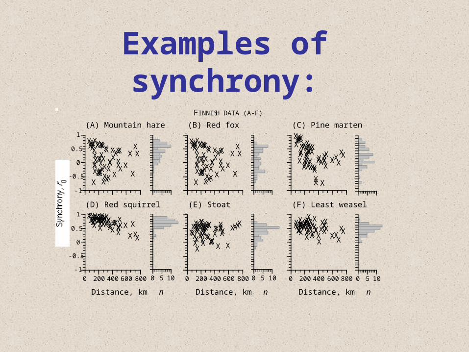
(A) Mountain hare (B) Red fox (C) Pine marten
(D) Red squirrel (E) Stoat (F) Least weasel
0 5 10 0 5 10 0 5 10
Distance, km n Distance, km n Distance, km n
FINNISH DATA (A-F)

Examples of synchrony:QuickTime™ and aGraphics decompressorare needed to see this picture.
SNOWSHOE HARE IN CANADA
(B)
(A)
X
X
X
X
X
X
X
XXX
X
X
X
X
X
X
X
X
X
X
X
X
X
X
X
XX
X
X
XXXXX
X
X
X
X
X
X
X
X
X
X
X
X
X
X
XX
XXXX
X
X
X
X
X
XX
X
X
X
X
X
X
XX
X
X
XX
X
X
X
X
XX
XX
X
X
X
X
X
X
X
X
X
X
X
X
XXXXX
X
X
X
XX
X
X
X
X
XX
X
X
X
X
XX
X
X
X
X
XX
X
XX
X
X
X
X
XX
XX
X
X
X
X
X
X
X
XX
XXX
X
X
XX
X
X
X
XX
X
X
X
X
X
X
X
X
X
X
X
XX
X
X
XX
X
X
X
X
X
X
XX
XX
X
X
XX
X
XX
X
X
X
X
X
X
X
X
XX
XX
X
XX
XX
X
X
X
XX
X
X
XX
XX
XX
X
XX
X
X
X
X
X
X
X
X
X
X
X
X
X
XXXX
X
X
X
X
X
X
X
X
XX
X
XX
X
XX
X
XX
X
X
X
XX
XXX
X
X
X
X
X
X
XX
X
X
X
X
XXX
X
X
X
X
XX
X
XX
XXX
X
X
X
X
X
XX
X
X
XX
X
X
X
XX
X
X
X
XXXX
X
X
X
X
X
XX
XXX
X
XX
X
X
X
XX
XXX
X
XX
XX
XX
X
X
X
X
XX
X
X
X
X
X
X
XX
X
X
X
X
XX
X
X
X
X
X
X
X
X
X
X
X
X
XX
XX
XX
X
X
X
XX
X
X
X
XXXX
X
XX
X
XX
X
X
X
XX
X
X
XX
X
XXX
X
X
X
X
XX
X
X
X
XX
XXX
XXX
X
X
X
X
X
X
X
XXX
X
X
X
XX
X
X
X
X
X
XX
X
X
X
X
X
X
X
XXXX
X
X
X
XX
X
X
X
X
XX
X
X
X
XX
XX
X
X
X
XX
X
X
X
XX
X
X
X
X
X
X
X
XXX
X
X
X
X
X
X
X
X
X
X
X
X
XXX
XX
X
X
X
X
XX
XX
X
X
X
XX
X
X
X
X
XX
X
XX
X
X
X
X
X
X
X
X
X
X
X
XX
XXXX
X
X
XX
X
X
X
XXX
X
X
XX
X
XX
X
XX
X
X
XX
X
X
X
X
XX
X
X
X
X
X
X
X
XXX
X
X
X
X
XX
X
X
X
X
X
X
XX
X
X
X
X
X
X
X
X
X
X
X
X
X
XXX
X
X
X
X
XX
X
XX
XXX
X
XX
X
X
X
XX
X
X
X
X
X
X
X
X
X
XXX
XX
X
X
X
X
X
X
X
X
X
X
X
X
XX
X
X
X
X
X
X
X
X
X
X
X
X
X
X
XX
XX
X
XXX
X
X
X
XX
X
XX
X
XXX
X
XX
X
XXX
X
X
X
XX
XX
X
X
X
XX
X
X
X
X
X
X
X
X
X
X
X
X
X
XXXX
X
X
X
X
X
X
X
X
X
X
X
X
X
X
XX
X
X
X
X
X
X
XX
X
X
X
XX
X
X
X
XX
X
XX
XXXX
X
X
X
X
X
X
X
XXX
X
X
X
X
XX
X
XXXXX
XX
X
X
X
X
X
X
X
XX
XX
X
X
X
X
X
X
X
X
X
X
XXX
X
X
XX
X
XXX
X
X
X
XXXXX
X
XX
X
X
XXXX
X
X
X
X
XXX
XXX
X
X
XX
X
X
X
X
X
X
X
X
X
X
X
X
X
X
X
XXX
XX
X
X
X
X
X
X
XX
X
XX
X
XX
X
X
X
X
X
X
XX
X
XX
X
X
X
XX
X
X
X
X
X
XXX
XX
X
X
X
X
X
X
X
X
X
X
XX
X
X
X
X
X
X
X
X
X
X
X
X
X
XX
X
X
XX
X
XXXX
XX
X
X
X
X
X
X
X
X
XXXX
X
X
X
XX
X
XX
X
X
X
X
X
XXXX
1
0.5
0
-0.5
-10 10 20 30
Distance, in grid units

Examples of synchrony:QuickTime™ and aGraphics decompressorare needed to see this picture.
0
10
20
0
10
20 J InsectsÉ Fish, crabH Birds
U Terrestrial vertebrates
A
Key:
0
0.2
0.4
0.6
0.8
-1 -0.8 -0.6 -0.4 -0.2 0 0.2
B
r = –0.34
0 10 20
C
Correlation betweensynchrony and distance, rD
Frequency, %

Two explanations of synchrony:
• P.A.P. Moran suggested (1953) that stochastic density-independent but correlated processes may cause local populations with a common structure of density dependence to fluctuate synchronously
X1(t+1) = aX1(t) + bX1(t–1) + (t)
X2(t+1) = aX2(t) + bX2(t–1) + (t)
– a and b are identical for X1 and X2
– the random elements and are different but correlated
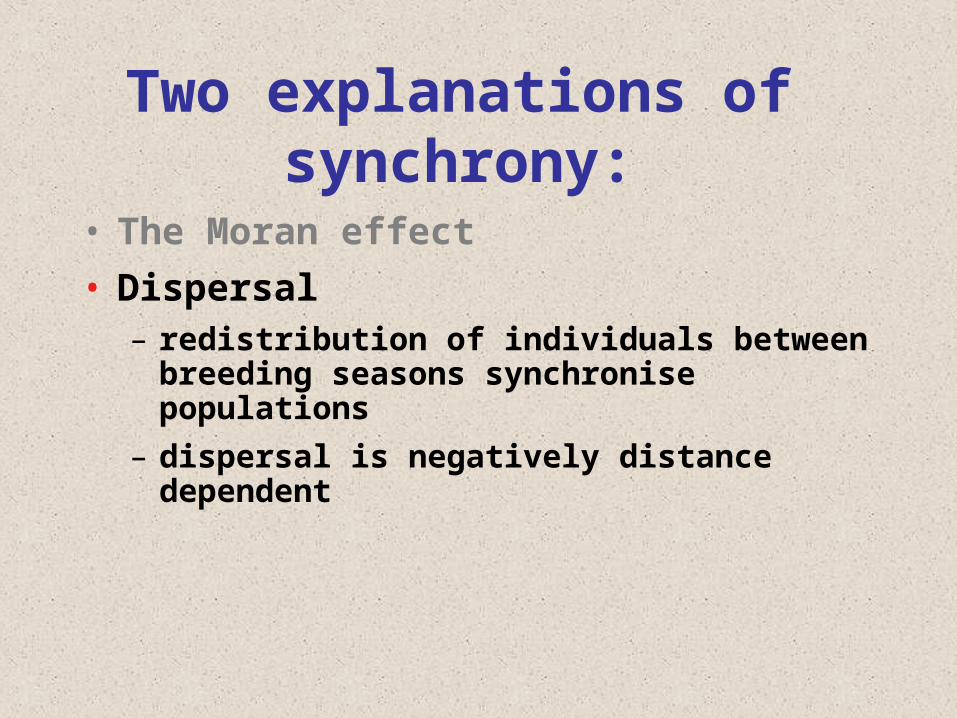
Two explanations of synchrony:
• The Moran effect
• Dispersal– redistribution of individuals between breeding
seasons synchronise populations
– dispersal is negatively distance dependent

Two explanations of synchrony:
The Moran effect and dispersal may act alone or in concert
QuickTime™ and aGraphics decompressorare needed to see this picture.
J
J
J
J
J
J
J
J
JJ
J
JJ
J J
JJJ J
JJ
JJ J
JJ
J
JJ
JJ
J
J
J
J
J
-1
-0.5
0
0.5
1
0 4 8 12
J
JJ
J JJ
JJ JJ
J
J
J
J
JJJJ J
J
JJ JJJJ
JJ
JJ
J
JJ JJ J
0 4 8 12
J
J
J
J
J J
J
J
JJ
J J
J J
J
J
J
J
J
JJ
J
JJ
JJ
JJ
JJ
J
J
J
J
J
J
0 4 8 12
J
J
J
J
JJ
J
J
JJJ J
J JJ
JJ
J
JJ
JJ
JJ
JJ
J JJ
JJ
JJ JJ J
0 4 8 12
Distance
(A) No MoranNo Dispersal
(B) Yes MoranNo Dispersal
(C) No MoranYes Dispersal
(D) Yes MoranYes Dispersal

Conclusion:
• Many animal populations (insects, fish, crustacean, mammals, birds) display synchronised population fluctuations over large geographical ranges

Conclusion:
• Many animal populations (insects, fish, crustacean, mammals, birds) display synchronised population fluctuations over large geographical ranges
• Often the level of synchrony goes down with increasing distance between the localities where the population data are collected

Conclusion:• Many animal populations (insects, fish, crustacean, mammals, birds) display synchronised population
fluctuations over large geographical ranges
• Often the level of synchrony goes down with increasing distance between the localities where the population data are collected
• These conclusions appear to be valid for seed set and flowering in perennial plants (Koenig et al., Post et al. in [too] numerous papers 1998 - 2001)

Comment:
• As to flowering plants,– Moran effect can synchronise life history events (flowering, seed set [masting])
– Dispersal is less likely to be valid here, unless there is local pollen limitation and pollen dispersal is negatively distance dependent

Comment:• As to flowering plants,
– Moran effect can synchronise life history events (flowering, seed set [masting])
– Dispersal is less likely to be valid here, unless there is local pollen limitation and pollen dispersal is negatively distance dependent
• The question is:
Can we build a simple model to explain life history synchronisation in perennial flowering plants?
Here the IBM models may come to a rescue

An IBM model for life history synchronisation:
• The model is built on individual-level accumulation of energy reserves i,k(t) in a given site k for flowering and reproduction

An IBM model for life history synchronisation:
• The model is built on individual-level accumulation of energy reserves i,k(t) in a given site k for flowering and reproduction
• The reserves are annually updated due to solar energy received during growing season

An IBM model for life history synchronisation:
• The model is built on individual-level accumulation of energy reserves i,k(t) in a given site k for flowering and reproduction
• The reserves are annually updated due to solar energy received during growing season
• The energy received is stand-level Ek(t) radiation topped off with i,k(t), variation individuals are experiencing due to, e.g., shading and wind factors affecting local spots
• Reproduction takes place once the accumulated reserve exceeds the threshold k for reproduction
• The reserves are depleted during reproductive bouts

An IBM model for life history synchronisation:
Threshold for flowering
Individual# 1
Individual# 2
En
erg
y le
vel
En
erg
y le
vel

An IBM model for life history synchronisation:
Threshold for flowering
Individual# 1
Individual# 2
En
erg
y le
vel
En
erg
y le
vel
An
nu
al E
An
nu
al E

An IBM model for life history synchronisation:
Threshold for flowering
Individual# 1
Individual# 2
En
erg
y le
vel
En
erg
y le
vel
An
nu
al E
An
nu
al E
Local

An IBM model for life history synchronisation:
Threshold for flowering
Individual# 1
Individual# 2
En
erg
y le
vel
En
erg
y le
vel

An IBM model for life history synchronisation:QuickTime™ and aGraphics decompressorare needed to see this picture.
Locality, k
Locality, k + 1
Locality, k + N
...
Πi,k + N(t)
Individual treesinluenced by
εi,k+ N(t)
Πi,k + 1(t)
Individual treesinluenced by
εi,k+1(t)
Πi,k(t)
Individual treesinluenced by
εi,k(t)
Inluenced bythe
Moran effect
Inluenced bythe
Moran effect
Inluenced bythe
Moran effect
Receiving Ek + N(t)
Threshold Φk + N
Receiving Ek + N(t)
Threshold Φk + 1
Receiving Ek + N(t)
Threshold Φk
Structure of the threshold model for reproduction

An IBM model for life history synchronisation:
0 10 20 30 40 50 60 70 80 90 1000
50
100
150
Individuals 1 - 100
0 10 20 30 40 50 60 70 80 90 1000
50
100
150
Individuals 1 - 100
0 10 20 30 40 50 60 70 80 90 1000
50
100
TIME
Ene
rgy
afte
r flo
wer
ing
befo
re f
low
erin
g%
flo
wer
ing

An IBM model for life history synchronisation:QuickTime™ and aGraphics decompressorare needed to see this picture.
-1
-0.5
0
0.5
1(a) E(t) = 100, Φ = 199
-1
-0.5
0
0.5
1
0 2 4 6 8 10
(b) E(t) = 100, Φ = 201
(c) E(t) = 100, Φ = 300
0 2 4 6 8 10
(d) E(t) = 100, Φ = 500No
stochasticity
With 5% of εi,k(t)
Time lag, years

• With no annual variation in Ek(t) and with no individual differences in energy accumulation due to local differences we find the following:
• When Ek(t) > all individuals in all sites will reproduce every year, with < Ek(t) < 2k reproduction in each k is synchronous with period two
• Whereas with Ek(t) << k the period length starts to increase
An IBM model for life history synchronisation:

QuickTime™ and aGraphics decompressorare needed to see this picture.
-0.5
0
0.5
1
-0.5
0
0.5
1
-0.5
0
0.5
1
1 0.9 0.8 0.7 0.6 0.5 1 0.9 0.8 0.7 0.6 0.5
NO STOCHASTICITY INDIVIDUALSTOCHASTICITY
Gradient similarity, d
1 0.9 0.8 0.7 0.6 0.5
MORAN EFFECT &INDIVIDUAL
STOCHASTICITY
Gradient differences in reproduction threshold,
Φ
Gradient differences in annual radiation, Ek(t)
Gradient differences in Φ and Ek(t)Matching
slope
Slope
differences
(a)
(d)
(g)
(b)
(e)
(h)
(c)
(f)
(i)

• By introducing differences (a) in Ek(t), assuming, e.g., a south – north gradient, will break down synchronous reproduction between any two groups where the difference in Ek(t) is large enough to cause flowering periodicities among the sites to differ.
• With gradient differences (b) in k reproduction will be asynchronous. Naturally, Ek(t) and k can (c) covary along the gradient
• Synchronous reproduction will be maintained among the sites until site-specific periodicities will start to change
An IBM model for life history synchronisation:

• Introducing stochasticity in i,k(t) under (a), (b) or (c) will break down regional reproductive synchrony
• Introducing a global modulator, the Moran effect, influencing i,k(t) of each individual in a matching manner, recovers synchronicity
An IBM model for life history synchronisation:

Conclusions:• We have created an individual based model on
reproduction in flowering plants
• With Moran effect the model is capable of producing synchronised life reproduction among separate populations
• With an environmental gradient in energy received or threshold of energy needed for reproduction one can get the level of synchrony going down against distance along the gradient
• This matches observations with real plants (seed set: W. Koenig et al.; flowering: E. Post et al.)