large scale earthquake parcel classification mapping for...
TRANSCRIPT

Page 1 of 66
Large scale earthquake parcel classification mapping for increasing public
safety and enhancing planning and development within Clark County, NV
By
Optim Seismic Data Solutions, Inc
200 S. Virginia Street, Suite 560
Reno, NV 89501
and
6255 McLeod DR Suite #6
Las Vegas, NV 89120
FOR
Board of Regents, Nevada System of Higher Education
University of Nevada, Reno
Reference: Prime Award No. PO 4800000057-017, Subaward No. UNR-08-03
September, 2010

Page 2 of 66
Summary
Optim Seismic Data Solutions via a subcontract from the Nevada System of Higher Education
(NSHE) measured shallow shear-velocity velocities throughout the approximately 500 square
miles of Clark County as part of contract from Clark County Department of Development
Services. In all, 9006 individual seismic arrays/lines were deployed and spatially located using
Geographical Positioning System (GPS) in a systematic manner in order to maximize the data
density coverage of the database within Clark County. Typically, these non-intrusive linear
arrays were about 604 feet in total length and consisted of 24 equally spaced channels using a
single 4.5Hz vertical geophone at each channel. Seismic microtremor measurements, mainly in
the form of ambient noise from traffic, were recorded for an average of 20 to 30 minutes at each
location/array. Noise recordings were then processed and analyzed using the refraction
microtremor (ReMi) method and a single shear wave velocity profile was determined for each
seismic array. These profiles were then used to calculate Vs100’ (or Vs30m) the average shear
wave velocities down to 100 feet per IBC 2006 equation 16-41. Once these were determined, the
information was concatenated with the GPS spatial data into a single Geographical Information
Systems (GIS) seismic database which was used to model Vs100’ across Clark County.

Page 3 of 66
Contents
1.0 Introduction ............................................................................................................................... 4
2.0 Methods Used ........................................................................................................................... 5
3.0 Seismic data acquisition procedure:........................................................................................ 11
3.1 Seismic array location selection .......................................................................................... 12
3.1.1 Permits ......................................................................................................................... 13
3.2 Seismic array (line) deployment ......................................................................................... 25
3.3 Data acquisition ................................................................................................................... 26
3.4 Array coordinates and documentation................................................................................. 26
3.5 Array re-deployment and data upload ................................................................................. 26
4.0 Seismic data processing .......................................................................................................... 26
4.1 Modeling constraints ........................................................................................................... 28
4.1.1 Shortened arrays........................................................................................................... 28
4.2 Site Class Examples ............................................................................................................ 29
4.3 Shape of the dispersion curves ............................................................................................ 40
4.4 Quality Assurance of the Results ........................................................................................ 46
4.4.1 Blind Tests ................................................................................................................... 48
4.5 Velocity Reversals............................................................................................................... 51
5.0 Results: Microzonation Map ................................................................................................... 58
6.0 Other Deliverables .................................................................................................................. 62
7.0 Conclusions and Recommendations ....................................................................................... 62
8.0 References ............................................................................................................................... 62
Appendix A (on DVD): Microzonation Map produced by krigging using the Vs100’ values as
per IBC Site Class equation 16-41 Section 1613.5.5. The steps used for krigging is also
enumerated.
Appendix B (on DVD): One-dimensional (1D) shear wave (Vs) velocity models, and IBC
Vs100’ (Vs30m) at test locations. An illustration of the associated dispersion curve is also
included.
Appendix C (on DVD): GIS referenced shapefile map showing the Vs100’, Vs20’ and values
representing the average velocities calculated using IBC equation 16-41 (Table 2) for the top
100’, 20’ and 10’ for all Clark County seismic array lines.
Appendix D: List of seismic arrays for which geometry information was collected.

Page 4 of 66
1.0 Introduction
The Nevada System of Higher Education (NSHE) was contracted by Clark County Department
of Development Services (CCDDS) to create a soil classification map based on site-specific
shear-wave velocities (“microzonation map”) of the County (Figure 1). NSHE subcontracted
Optim SDS to perform this work under their supervision. Optim SDS employed the SeisOpt®
REfraction MIcrotremor (“ReMi”™) method to create the microzonation map. ReMi (Louie,
2001) is a non-intrusive, passive technique that uses ambient noise as its source.
Figure 1: Area within Clark County to be mapped for earthquake parcel classification. The County defined and
prioritized specific areas to be mapped.
Measurement of shear-wave velocity (Vs) in the shallow subsurface is essential for the
estimation of seismic hazard, the development of seismic-hazard maps, and the calibration of
recorded ground motion data. The site class measurements are represented by the average shear
wave velocity value for the top 100 feet or 30 meters (Vs100’ or Vs30m) as per IBC 2006
Section 1613.5.5. It is an integral to seismic design of structures per the International Building
Code and International Residential Code, (IBC) and (IRC) respectively. Site class directly
determines the Seismic Design Category (SDC) used by structural engineers and if not otherwise
determined through an approved test method, engineers must revert to the default site class.
Often this means adhering to a more stringent site class than the actual ground conditions would

Page 5 of 66
dictate and indirectly drives up the cost of design. Therefore, knowing the actual Vs100’ (or
Vs30m) values across Clark County can provide essential data necessary for seismic hazard
mitigation and also provide a direct cost savings for new construction and in the retrofitting of
existing buildings.
Based on this GIS seismic database, the project was intended to provide Clark County a single
shear-wave velocity based map with contoured values corresponding to the site classifications of
the IBC and National Earthquake Hazards Reduction Program (NEHRP) definitions for site
class, (Table 1). Furthermore, in collaboration with the City of Henderson (CoH) Building
Department, both velocity databases from the CCDDS and the CoH were integrated into a single
Vs database and the interpolated velocity map was based on the entire joint database to provide
seamless interpolation across the CCDDS and CoH boundaries. This velocity map will provide
city planners, building officials, design professionals, and researchers alike the opportunity to
determine the actual site class value of a particular parcel before a single site specific
investigation is performed.
Optim SDS performed all necessary tasks for completion of the work, including field data
acquisition, data processing and reports, working with University personnel to make the products
of the work available in a format to be mutually agreed upon during the term of this contract. As
part of the project, data from a total of 9006 sites were acquired, processed and submitted to the
City. This represents 100% of the total number of seismic lines (~9000) scheduled to be
collected as part of this project.
2.0 Methods Used
Optim SDS measured shear velocity as a function of depth at each of the locations using the
refraction-microtremor (ReMi) surface array technique. Louie (2001) developed the refraction
microtremor technique (commercially available as SeisOpt®ReMi
TM, © Optim 2001-2010) as a
more rapid and cost-effective method of measuring Vs30m to meet the IBC code (BSSC, 1997),
and to derive site conditions. This method has been peer reviewed and blind tested against both
borehole and multi-channel analysis of surface waves (MASW) (Louie, 2001; Stephenson et al.,
2005; Thelen et al., 2006). Refraction microtremor is a volume-averaging surface-wave
measurement, averaging velocities where geology is laterally variable, thus providing a more
appropriate measure of site effects on earthquake wave propagation than single-point data
obtained from downhole logs.
The essence of the ReMi technique is that ambient noise contains a usable signal that is
predictable from the velocity structure that is presumably caused mainly by human activities
(e.g. trucks, trains, and airplanes, human activity either induced or natural). Microtremor noise
from these sources excites Rayleigh waves, which are recorded by a linear array of 24 vertical
refraction geophones (Figure 2). The data acquisition procedure consists of obtaining 10-15, 30-
second sampled at 2 milliseconds (Figure 3). The Rayleigh waves contained in the recorded
microtremors (ambient noise) are separated from other wave arrivals using a two dimensional
slowness–frequency (p–f) transform of the noise records. The fundamental-mode phase-velocity
Rayleigh wave dispersion curve is picked along the minimum velocity of the energy envelope
within the slowness–frequency spectral image (Figure 4B). The spectrum is normalized as the

Page 6 of 66
ratio of the power spectrum at a particular frequency and slowness (inverse velocity) over the
average value for all slowness values at that frequency. Modeling of the dispersion curve (Figure
4A) produces a depth–velocity model (Figure 4C) that can be vertically averaged to the single
Vs30m value used by the IBC code (Table 2). The preferred profile will always be the profile
interpretation that results in the minimum number of layers to accommodate the observed
Rayleigh-wave dispersion and produces a best estimate, reliable and repeatable velocity
structure.
The IBC Site Class is calculated using the equations provided in the International Building Code
book. The following sections are extracted from its pages. Note that even though Vs100’ values
(average velocities as determined from equation 16-41 below) may give you an average
velocity that is Site Class B, the criteria defined in the IBC code book must be used (Table
3).
Table1: Table 1613.5.5 from 2006 International Building Code. This and the criteria described below must be used
to determine Site Class from the Vs100 values obtained during the project.

Page 7 of 66
Table2: Extract from 2006 International Building Code that shows how the Vs100’ that is used to determine Site
Class is calculated.

Page 8 of 66
Table3: Extract from 2006 International Building Code explaining the criteria used to classify a site. Note that Site
Classes A and B have to be further verified by a geotechnical engineer as described above.

Page 9 of 66
Figure 2: Refraction geophones (red sensors in picture) are placed on sidewalks or along paths to record ambient
noise generated by traffic, people walking or any other energy generated by active or passive source.
Figure 3: Ambient noise is recorded and analyzed to determine one-dimensional (1-D) shear wave velocity profile
(Figure 4) beneath each seismic profile.

Page 10 of 66
Figure 4: Recorded ambient (microtremor) data are first transformed into the frequency-slowness domain (Louie,
2001) (A). The dispersion curve is then picked (B) and modeled to obtain a 1D shear-wave velocity profile (C).
Vs=3255
Site Class B
b237s05_28
C
B
A

Page 11 of 66
3.0 Seismic data acquisition procedure:
The following summarizes the data acquisition procedure for the project. Data acquired is
processed using the SeisOpt® ReMi™ (© Optim, Inc) software to obtain the Vs30m (average
velocities in the top 100 feet as defined by IBC) values and the shear-wave velocity profile down
to a depth of 100 feet.
Data was collected throughout Clark County using the microtremor method (Louie, 2001). Field
crews were deployed with all necessary equipment, including: seismographs, GPS receivers,
seismic cables, geophones, hammer and strike plate, and laptops in both urban and rural settings
in two to four person teams. Site locations typically were reached via street approved vehicles,
off highway vehicles (OHV), and hiking, then placed alongside roadways, trails, open fields, or
open desert. During mission planning, crews would determine the appropriate equipment type,
modes of egress and digress, and the best data collection times depending on terrain conditions,
land use regulations, traffic conditions, and property owner stipulations, all in an effort to
minimize any potential impact to the environment and infrastructure while maximizing safety
and reducing any disturbances to the public. In some instances, special authorization had to be
obtained and site specific training requirements had to be met before accessing these site
locations. Optim SDS worked in concert with Clark County, local and federal government
entities, and property owners to adhere to all arrangements and conditions set forth and to obtain
any required permits before data collection was conducted.
In theory, the accuracy and the resolution of any model is a direct function of the data density of
the database. In determining the appropriate data density to be used, Optim SDS utilized
Southern Nevada Technical Guidelines as a basis for data density of 1 velocity sample per 36
acres. To aid in the capturing of evenly dispersed data, based on 1/36 acres, Optim SDS,
CCDDS, and the CoH internally developed a gridded subsection scheme based on the existing
book and section projections of Nevada (Figure 5). These GIS generated subsection layers were
loaded up onto the handheld GPS devices that were deployed to the field and helped guide data
collection efforts. However, due to limitations imposed by natural terrain, inaccessible areas,
large structures, and infrastructure obstructions, the data density across the entire project area
varied, rendering the 1/36 acre data density more of a guideline than an absolute standard. In
addition, in several areas, due to proximity to key infrastructure, identified geology of interest,
and velocity anomalies discovered in the data set as the project progressed, data density was
increased to better define the interpolated modeled surface in those areas. For instance, seismic
array locations were intentionally placed with strategic orientation in mind, crossing known
faults and fissure zones when possible. In order to maximize the potential to actually cross any
subsurface fault or fissure related features, arrays were placed perpendicular to the assumed
projected strike when possible.

Page 12 of 66
3.1 Seismic array location selection
All seismic array locations are intended to maintain an average test coverage or data density of 1
array per 36 acres with no less than 1000 feet measured midpoint to midpoint between each
array location. Utilizing an internally established grid (Figure 5) as a point of reference and aerial
photographs with the occasional site reconnaissance, a general site location is selected before the
array deployment.
Figure 5: Schematic showing section map subdivided into 36 sub-sections and odd numbers shaded for better
reference.
The established grid is based directly off the corresponding Township & Range associated with
the project area. Thus, each township equals 1-book, each book equals 36-square miles, and each
square mile or section is further divided down to 36 sub-sections. Each sub-section is
approximately 880 feet by 880 feet or approximately 17.7 acres. Therefore, we attempt to
perform a seismic array in 18 of the 36 sub-sections per section or 1 seismic array per 36 acres.
However, due to projection limitations some subsections are distorted, but the data density is
uniform.
The location of the seismic array is further refined on the following conditions encountered at the
proposed location:
Safety concerns
o High traffic and/or speed limit hazards
o Construction zones
Site overall accessibility:

Page 13 of 66
o Private property concerns
o Shoulder area and vehicle accessibility
o Array length of 604 feet to location length (does the line fit)
o Up to 2 channels may be omitted from the array (under cetain circumstances)
o Driveways (residential and commercial)
o Some driveways can be “bridged” with a hard line and others must be crossed
using wireless techniques.
Ambient noise and line geometry
o Relative slope and curvature of the array
o Parallel noise sources are preferred
o Very high energy perpendicular sources are avoided.
Other concerns
o Artificial underground voids (overpasses, tunnels, drainage channels, etc..)
3.1.1 Permits
As part subcontract to conduct thousands of site condition measurements for Clark County,
Optim SDS has gained access to several secure locations. These are listed below:
1. Bali Hai Golf Club
Location: 5160 Las Vegas Blvd. South
Las Vegas, NV 89119
Site website: www.balihaigolfclub.com
Google website: http://maps.google.com/maps?hl=en&ie=UTF8&ll=36.079835,-115.177531&spn=0.0154,0.043774&t=h&z=15
Permit required: No
Notes:
Cold called course General Manager.
Was put in touch with corporate office managing three of the local courses.
Arranged evening access.
2. Durango Hills Golf Club
Location: 3501 N. Durago Drive
Las Vegas, NV 892129
Site website: www.durangohillsgolf.com
Google website: http://maps.google.com/maps?hl=en&ie=UTF8&ll=36.222932,-115.281687&spn=0.007686,0.021887&t=h&z=16
Permit required: No
Notes:
Cold called course Manager.
Arranged early morning access through maintenance manager.
3. Angel Park Golf Club
Location: 100 South Rampart Blvd
Las Vegas, NV 89145
Site website: www.angelpark.com
Google website: http://maps.google.com/maps?hl=en&ie=UTF8&ll=36.177583,-115.288038&spn=0.015381,0.043774&t=h&z=15

Page 14 of 66
Permit required: No
Notes:
Cold called Manager.
Arranged course access on off day through course maintenance manager.
4. Royal Links Golf Club
Location: 5995 E. Vegas Valley Dr.
Las Vegas, NV
Site website: www.royallinksgolfclub.com
Google website: http://maps.google.com/maps?hl=en&ie=UTF8&ll=36.133456,-115.049193&spn=0.007695,0.021887&t=h&z=16 Permit required: No
Notes:
Cold called course Manager.
Arranged access to maintenance road.
5. Wynn Country Club
Location: 3131 Las Vegas Blvd. S
Las Vegas, NV 89109
Site website: www.wynnlasvegas.com
Google website: http://maps.google.com/maps?hl=en&ie=UTF8&ll=36.125934,-115.159464&spn=0.007695,0.021887&t=h&z=16
Permit required: No
Notes:
Cold called course Manager.
Worked through several different company divisions before given permission by legal
department.
Arranged early morning access though course maintenance manager.
6. Wild Horse Golf Club
Location: 2100 Warm Springs Road
Henderson, NV 89014
Site website: www.golfwildhorse.com
Google website: http://maps.google.com/maps?hl=en&ie=UTF8&ll=36.059456,-115.077646&spn=0.007702,0.021887&t=h&z=16 Permit required: No
Notes:
Cold called course Manager.
Arranged through course maintenance manager.
No special time for access required.
7. Black Mountain Golf Club
Location: 500 Greenway Road
Henderson, NV 89015
Site website: http://www.golfblackmountain.com/golf/proto/golfblackmountain/
Google website: http://maps.google.com/maps?hl=en&ie=UTF8&ll=36.016147,-114.971387&spn=0.007706,0.021887&t=h&z=16
Permit required: No

Page 15 of 66
8. Black Mountain Industrial Complex
a. Olin Chor Alkali Products
Location: 8000 Lake Mead Parkway
Henderson, NV 89009
Site website: www.olinchloralkali.com
Google website: http://maps.google.com/maps?hl=en&ie=UTF8&ll=36.041118,-115.003338&spn=0.015407,0.043774&t=h&z=15
Permit required: No
Notes:
Cold called plant manager.
Met with plant manager, assistant manager and safety officer.
Field crew was required to attend regularly scheduled weekly training and to meet PPE
requirements.
b. Timet
Location: 8000 Lake Mead Parkway
Henderson, NV 89009
Site website: www.timet.com
Permit required: No
Notes:
Cold called plant manager.
Met with plant manager and safety officer.
Field crew was required to attend safety training and meet PPE requirements.
c. Basic Remediation Company
Location: 873 West Warm Springs
Henderson, NV, 89011
Permit required: No
Notes:
Cold called plant manager.
Met with operations manager to coordinate data collection times and identify areas that
were non-accessible.
Data collection was limited in scope due to lack of access from environmental concerns.
9. Clark County Water Reclamation main facility
Location: 8556 East Flamingo Road
Las Vegas, NV, 89122
Site website: www.cleanwaterteam.com
Google website: http://maps.google.com/maps?hl=en&ie=UTF8&ll=36.111669,-115.04149&spn=0.015393,0.027423&t=h&z=15
Permit required: No
Notes:
Cold called, was referred to several people, before given permission.
10. Rivers Mountain Water Treatment Facility
Location: 1299 Burkholder Blvd
Henderson, NV, 89015

Page 16 of 66
Site website: www.snwa.com
Google website: http://maps.google.com/maps?hl=en&ie=UTF8&ll=36.026091,-114.926863&spn=0.01541,0.027423&t=h&z=15 Permit required: No
Notes:
Cold called the facility, talked with security.
Talked with Head of Security.
Helped access another small area of land to the north.
Field crew was required to attend brief safety training.
11. Nevada Energy
Site website: www.nvenegry.com
a. Clark Substation Location: N. Stephanie St, Las Vegas, NV
Google website: http://maps.google.com/maps?hl=en&ie=UTF8&ll=36.087725,-115.050159&spn=0.007699,0.013711&t=h&z=16
Permit required: No
Notes:
Stopped by at guard station and got phone number for central office, talked with several
people before being given number of plant manager.
Field crew was required to attend safety briefing and meet PPE requirement.
b. Walter M. Higgins Generating Station
Location: East Primm Blvd, Primm, NV
Google website: http://maps.google.com/maps?hl=en&ie=UTF8&ll=35.614011,-115.355866&spn=0.007745,0.013711&t=h&z=16
Permit required: No
Notes:
Called contact at Nevada Energy and was given plant managers contact information.
Field crew was required to have an escort.
12. Mohave Generating Station
Location: Bruce Woodbury Dr, Laughlin, NV
Site website: http://www.sce.com/PowerandEnvironment/PowerGeneration/MohaveGenerationStation/
Google website: http://maps.google.com/maps?hl=en&ie=UTF8&ll=35.143494,-114.594612&spn=0.031162,0.054846&t=h&z=14 Permit required: No
Notes:
Cold called, and talk with plant manager
Met with plant manager, safety officer and chief engineer.
Granted access with the stipulation that Southern California Edison receives a copy of the
data.
Field crew was required to attend 2 hours of safety training and to inform the chief
engineer of work plans for the day.
13. Clark County Detention Basins
Location: Detention basins throughout the county
Site website: http://www.ccrfcd.org/

Page 17 of 66
Permit required: No
Notes:
Cold called Clark County Flood Control District, was able to talk with the person in
charge of maintaining the detention basins of which there are several throughout the
county
Field crew was allowed access to basin under the following stipulations: cannot drive
over 5 mph to avoid dust, cannot drive on the floor of the basins, and must keep gates
lock expect with entering and leaving
14. Henderson Executive Airport
Location: 3500 Executive Terminal Dr
Henderson, NV 89052
Site website: www.hnd.aero
Google website: http://maps.google.com/maps?hl=en&ie=UTF8&ll=35.972241,-115.135946&spn=0.030842,0.054846&t=h&z=14
Permit required: No
Notes:
Cold called the General Manager.
Contact information was relayed to Clark County Department of Aviation who contacted
OptimSDS.
A meeting was arranged to be attended by all interested parties (Airport Management,
OptimSDS management, and Werner from the county Building Department).
Field crew was required to have an escort while on site.
15. North Las Vegas Airport
Location: 2730 Airport Dr
North Las Vegas, NV 89032
Site website: http://www.vgt.aero/01-home.aspx
Google website: http://maps.google.com/maps?hl=en&ie=UTF8&ll=36.210139,-115.193281&spn=0.01624,0.043774&t=h&z=15 Permit required: No
Notes:
Made contact through Henderson Executive Airport.
Field crew was required to have an escort while on site.
16. Perkins-Overland Field
Site website: http://www.mccarran.com/ga_overton.aspx
Google website: http://maps.google.com/maps?hl=en&ie=UTF8&ll=36.56846,-114.445438&spn=0.016165,0.043774&t=h&z=15
Permit required: No
Notes:
Permission for access was given through North Las Vegas Airport.
17. Jean Sport Aviation Center
Site website: http://www.mccarran.com/ga_jean.aspx
Google website: http://maps.google.com/maps?hl=en&ie=UTF8&ll=35.77082,-115.325718&spn=0.032661,0.087547&t=h&z=14
Permit required: No
Notes:

Page 18 of 66
Permission for access was given through Henderson Executive Airport.
Field crew was required to have an escort while on site.
18. Big Bend State Recreation Area
Site website: http://parks.nv.gov/bb.htm
Google website: http://maps.google.com/maps?hl=en&ie=UTF8&ll=35.201025,-114.62122&spn=0.065787,0.175095&t=h&z=13
Permit required: No
Notes:
Field crew was granted access permission from onsite personnel.
19. Lead Mead National Recreation Area - see Figure 6 and 7 for map of permit areas.
Site website: http://www.nps.gov/lake/index.htm
Permit required: Yes
Notes:
Field crews were granted access per the permit and scheduled data collection with park
officials
a. Laughlin
Google website: http://maps.google.com/maps?hl=en&ie=UTF8&ll=35.192959,-114.613409&spn=0.032897,0.087547&t=h&z=14
Permit required: Yes

Page 19 of 66
Figure 6: Map showing permit areas in the Lake Mead national Park, north of Laughlin.

Page 20 of 66
a. Overton
Google website: http://maps.google.com/maps?hl=en&ie=UTF8&ll=36.527157,-114.457283&spn=0.064695,0.175095&t=h&z=13
Permit required: Yes
Figure 7: Map showing permit areas in the Lake Mead national Park, south of Overton.

Page 21 of 66
20. Coyote Springs - see Figure 8 for map of permit areas.
Site website: http://www.coyotesprings.com/
Google website: http://maps.google.com/maps?hl=en&ie=UTF8&ll=36.824127,-114.932613&spn=0.064446,0.175095&t=h&z=13
a. Pardee Homes (Developer)
Site website: http://www.pardeehomes.com/
Permit required: Yes
Notes:
Contacted the developer with help from the CCBD
Field crews were granted access per the Seismic Revocable License (8747_4.DOC) dated
April 27,2010.
Scheduling was on a daily basis with onsite officials.
b. Coyote Springs Investment (Land Owner)
Permit required: Yes,
Notes:
Field crews were granted access per Seismic Research Revocable License.:
SeismicLicense (v_4) 3-8-10
Scheduling was on a daily basis with onsite officials.

Page 22 of 66
Figure 8: Map showing permit areas in the Coyote Springs region.
21. Desert Tortoise Large Scale Translocation Site - see Figure 9 for map of permit areas.
Google website: http://maps.google.com/maps?hl=en&ie=UTF8&ll=35.739546,-115.365372&spn=0.130695,0.350189&t=h&z=12
Google website: http://maps.google.com/maps?hl=en&ie=UTF8&ll=35.979048,-115.241561&spn=0.016288,0.043774&t=h&z=15
Permit required: Yes
Notes:
Field crews were granted access per the permit NV-052-UA-10-08 dated Sep 24, 2010.
Scheduling was on a daily basis with BLM officials.
Figure 9: Map showing permit areas in the tortoise habitat region near Jean, NV.

Page 23 of 66
22. Lake Las Vegas - see Figure 10 for map of permit areas.
Site website: http://www.lakelasvegas.com/
a. North Shore
Google website: http://maps.google.com/maps?hl=en&ie=UTF8&ll=36.115829,-114.936991&spn=0.032519,0.087547&t=h&z=14
Permit required: Yes
Notes:
Access was granted per the Right of Entry Agreement No.: OSDS- (06.14.10) dated June
17, 2010.
Data collection was scheduled with onsite personnel.
b. South Shore
Google website: http://maps.google.com/maps?hl=en&ie=UTF8&ll=36.105844,-114.925575&spn=0.032523,0.087547&t=h&z=14
Permit required: No
Notes:
Various HOA's were individually contacted and access granted and data collection
scheduled through those specific HOA's. Assistance from the CoH was used.
Figure 10: Map showing permit areas in the Lake Las Vegas region.

Page 24 of 66
23. Hiking Areas in Book 192 North - see Figure 11 for map of permit areas.
Permit required: Yes
Notes:
Permission for these areas was piggy backed onto the Tortoise Permit, NV-052-UA-10-
08 dated Sep 24, 2010.
Scheduling was on a daily basis with BLM officials.
Figure 11: Map showing permit areas in the tortoise sanctuary region in book 192.

Page 25 of 66
24. Wetlands Park – Clark County Parks and Recreation.
Location: 7050 Wetlands Park Lane, Las Vegas, NV
Site website: http://www.accessclarkcounty.com/depts/parks/locations/pages/wetlands.aspx
Google website: http://maps.google.com/maps?hl=en&ie=UTF8&ll=36.097938,-115.016813&spn=0.032526,0.087547&t=h&z=14
Permit required: No
Notes:
Cold called facility supervisor.
Scheduled data collection through onsite personnel.
Field crew was granted access permission but had to remain on dirt roads while driving
vehicles.
25. Crystal Ridge (aka Ascaya)
Site website: http://ascaya.com/#/welcome_intro/
Google website: http://maps.google.com/maps?hl=en&ie=UTF8&ll=36.010297,-115.026512&spn=0.032562,0.054846&t=h&z=14
Permit required: No
Notes:
Contacted developer with help from the CoH.
Scheduled data collection through developer and coordinated with onsite personnel.
3.2 Seismic array (line) deployment
Seismic cables are deployed at the array location in a linear fashion.
Various configurations are possible, for example: 1*24 channels, 2*12 channels, 4*6
channels, etc.
Geophone spacing is built in to the cables at 8 meters (26.24 feet). This spacing is
consistent throughout all the project array sites unless otherwise specified.
Geophones (24 total) are deployed and connected to the seismic cable with a maximum
lateral tolerance equal to the individual geophone cable length or approximately 38
inches.
The geophones are planted at no more than 15° from vertical.
Up to 2 geophones may be deleted from a survey.
The curvature of the array is restricted to no more that 5% to 10%, depending on site
conditions, of the total array length before geometry information needs to be aquired.
The total elevation change across the array is limited to 5% to 10%, depending on site
conditions, of the array length before geometry information needs to be aquired.
Seismic data acquisition hardware is connected to the cable. (24-bit digital seismograph,
internal GPS, etc.)
Horizontal geometry was measured at each of the 24 geophones. A high resolution GPS
unit was used surveyed for latitude and longitude
Vertical geometry was measured at each of the 24 geophones using a high resolution GPS
unit or a leveling rod.
Geometry was obtained for 467 of the seismic arrays. These are listed in Appendtix D.
Geometries were applied to the data during data processing.

Page 26 of 66
3.3 Data acquisition
Once on a site, seismic arrays were deployed using linear arrays consisting of 24
geophones with 8 meters (26.24 feet) geophone spacing for a total array line length of
184 meters (603.67 feet).
Ambient noise microtremors were then recorded using standard vertical 4.5 Hz
geophones recorded at a rate of two milliseconds for intervals of 30 seconds each. In all, a
total of 12 to 20, 30 second recordings were collected for each seismic array. All raw
seismic data was collected utilizing Seismic Sources Company’s 24 channel, DAQLink II
digital seismographs and the seismic data acquisition system software VibraScope V2.4.12
or higher. Figure 3 depicts the field crew during actual data collection. In addition, hammer
hits using an 8 pound or 10 pound sledge and strike plate were collected at approximately
15 feet and 30 feet off both ends during normal passive data collection to increase high
frequency energy. This was especially useful in low energy environments, typically rural
settings away from traffic and other ambient noise sources.
During the acquisition phase, data is monitored for energy content of the ambient noise
and energy anomolies caused by power utilities, wind and other interferences that would
adversely affect the data.
Data irregularities are investigated in the field and corrected if possible and documented
if not.
3.4 Array coordinates and documentation
While data aquisition is being performed, the array endpoints are surveyed for latitude,
longitude, and elevation using a high resolution GPS. These coordinates provide a two-
dimensional orientation of the array with respect to geophones 1 and 24.
The first GPS point is recorded at geophone 1 and the second GPS point is recorded at
geophone 24.
In addition, a single digital photograph is taken of the fully deployed array to document
site conditions.
3.5 Array re-deployment and data upload
Once data aquisition and array documentation is completed all the seismic line hardware
is disconnected and properly stored for travel to the next array location. The data
collection procedure begins for the next seismic line from Section 3.1 of this document.
At the close of each day all data is uploaded for data processing and analysis.
If the uploaded data does not contain adequate Rayleigh-wave energy then a request may
be made to repeat the survey.
4.0 Seismic data processing

Page 27 of 66
The noise records collected above were processed using the SeisOpt® ReMi™ software (© Optim,
Inc., 2001-2008) that uses the refraction microtremor method (Louie, 2001). The refraction
microtremor technique is based on two fundamental ideas. The first is that common seismic-
refraction recording equipment, set out in a way almost identical to shallow P-wave refraction
surveys, can effectively record surface waves at frequencies as low as 1 Hz. The second idea is that a
simple, two-dimensional slowness-frequency (p-f) transform of a microtremor record can separate
Rayleigh waves from other seismic arrivals, and allow recognition of true phase velocity against
apparent velocities. Two essential factors that allow exploration equipment to record surface-wave
velocity dispersion, with a minimum of field effort, are the use of a single geophone sensor at each
channel, rather than a geophone “group array”, and the use of a linear spread of 24 geophone sensor
channels. Single geophones are the most commonly available type, and are typically used for
refraction rather than reflection surveying. The advantages of ReMi from a seismic surveying point
of view are several, including the following: It requires only standard refraction equipment; it
requires no triggered source of wave energy; and it will work best in a seismically noisy urban
setting. Traffic and other vehicles, and possibly the wind responses of trees, buildings, and utility
standards provide the surface waves this method analyzes.
There were three main processing steps:
Step 1: Create a velocity spectrum (p-f image) from the noise data: The distinctive slope of
dispersive waves is a real advantage of the p-f analysis. Other arrivals that appear in microtremor
records, such as body waves and airwaves cannot have such a slope. The p-f spectral power image
will show where such waves have significant energy. Even if most of the energy in a seismic record
is a phase other than Rayleigh waves, the p-f analysis will separate that energy in the slowness-
frequency plot away from the dispersion curves this technique interprets. By recording many
channels, retaining complete vertical seismograms, and employing the p-f transform, this method
can successfully analyze Rayleigh-wave dispersion where SASW techniques cannot.
Step 2: Rayleigh-wave dispersion picking: Picking is done along a ``lowest-velocity envelope''
bounding the energy appearing in the p-f image. This ensures that the picks are representative of true
velocities rather than apparent velocities, since noise is assumed to come from all directions. Picking
a surface-wave dispersion curve along an envelope of the lowest phase velocities having high
spectral ratio at each frequency has a further desirable effect. Since higher-mode Rayleigh waves
have phase velocities above those of the fundamental mode, the refraction microtremor technique
preferentially yields the fundamental-mode velocities. Higher modes may appear as separate
dispersion trends on the p-f images, if they are nearly as energetic as the fundamental. Spatial
aliasing will contribute to artifacts in the slowness-frequency spectral-ratio images. The artifacts
slope on the p-f images in a direction opposite to normal-mode dispersion. The p-tau transform is
done in the space and time domain, however, so even the aliased frequencies preserve some
information. The seismic waves are not continuously harmonic but arrives in-groups. Further, the
refraction microtremor analysis has not just two seismograms, but 10 or more. Hence severe
slowness wraparound does not occur until well above the spatial Nyquist frequency which is about
twice the Nyquist in most cases.
Step 3: Shear wave velocity modeling: The refraction microtremor method interactively forward-
models the normal-mode dispersion data picked from the p-f images with a code adapted from Saito
Page 28 of 66
(1979, 1988) in 1992 by Yuehua Zeng. This code produces results identical to those of the forward-
modeling codes used by Iwata et al. (1998), and by Xia et al. (1999) within their inversion
procedure. The modeling iterates on phase velocity at each period (or frequency), reports when a
solution has not been found within the iteration parameters, and can model velocity reversals with
depth.
4.1 Modeling constraints
The preferred profile will always be the profile interpretation that results in the minimum number
of layers to accommodate the observed Rayleigh-wave dispersion and produces a best estimate,
reliable and repeatable velocity structure. Because forward modeling is used rather that an
inverse method to obtain our velocity-depth model, we are able to test the necessity and
sensitivity of the data to both layer thickness and layer velocity. The resultant model is therefore
the simplest to explain the data. This follows from Occam's razor principle that "entities must not
be multiplied beyond necessity", which simply states that “one should not increase, beyond what
is necessary, the number of entities required to explain anything”.
4.1.1 Shortened arrays
Due to artifacts resulting from topographic changes along the length of the array, some geophone
traces were required to be removed from analysis to allow more accurate determination of the
velocity structure. These arrays are:
2173606 geophones used: 1 to 15
2173618 geophones used: 13 to 24
Some remote areas were not accessible by vehicles or off highway vehicles (OHV). To access
these areas, equipment had to be hiked to each location. Due to the physical burden of the 604
foot seismic cable and site conditions, a shorter 230 foot long cable was utilized with 10 foot
spacing between each of the 24 geophones. There were 107 seismic arrays that were acquired
with 230 feet total length. These array lines are:
1233310 1261031 1261518 1402613 1920218 2172808
1233314 1261106 1261520 1402626 1920230 2172810
1260403 1261108 1261522 1601904 1920324 2172814
1260405 1261110 1261528 1601905 1920335 2172821
1260409 1261112 1261532 1601908 1920336 2172827
1260501 1261114 1261807 1601924 1923616 2172834
1260502 1261116 1261809 1601935 2040209 2173314
1260505 1261118 1261816 1602215 2171008 2230505
1260506 1261120 1261818 1603017 2171017 2230511
1260508 1261122 1261823 1613329 2171028 2230801
1260514 1261123 1261827 1640408 2171535 2230808
1260518 1261126 1262326 1640409 2171536 2230810
1260530 1261128 1262331 1640419 2172135 2230813
1260533 1261130 1400416 1640420 2172203 2231734

Page 29 of 66
1260713 1261132 1402413 1640422 2172205 2232014
1260806 1261134 1402424 1640430 2172222 2232034
1260925 1261508 1402425 1920205 2172232 2232910
1261019 1261516 1402601 1920216 2172719
Despite the shorter line lengths, the Raleigh-wave dispersion data still contained sufficient detail
to enable a 100 foot velocity profile to be obtained.
4.2 Site Class Examples
Vertically averaged shear-wave velocities resulted in single Vs30m values which corresponded
to sites class B, C, and D as defined by the IBC code (see Table 2). The following are examples
of data from each of these three site classes.
Site Class B examples are shown in Figures 12, 13, 14 and 15. Note that here Site Class B is
defined based just on the velocities. The criteria described in Table 3 is must be used on a
site by site case to make sure it can be classified as Site Class B.
Site Class C examples are shown in Figures 16, 17 and 18.
Site Class D examples are shown in Figures 19, 20, and 21.

Page 30 of 66
Figure 12: Example of Site Class B data as determined from velocities ONLY. Recorded microtremor data are
first transformed into the frequency-slowness domain (Louie, 2001) (A). The dispersion curve is then picked (B) and
modeled to obtain a 1D shear-wave velocity profile (C).
Vs=2732
Site Class B
b191s18 _21
A
B
C

Page 31 of 66
Figure 13: Example of Site Class B data as determined from velocities ONLY. Recorded microtremor data are
first transformed into the frequency-slowness domain (Louie, 2001) (A). The dispersion curve is then picked (B) and
modeled to obtain a 1D shear-wave velocity profile (C).
Vs=3288
Site Class B
b125s18_08
C
B
A

Page 32 of 66
Figure 14: Example of Site Class B data as determined from velocities ONLY. Recorded microtremor data are
first transformed into the frequency-slowness domain (Louie, 2001) (A). The dispersion curve is then picked (B) and
modeled to obtain a 1D shear-wave velocity profile (C).
Vs=2556
Site Class B
b216s30_07
C
B
A

Page 33 of 66
Figure 15: Example of Site Class B data as determined from velocities ONLY. Recorded microtremor data are
first transformed into the frequency-slowness domain (Louie, 2001) (A). The dispersion curve is then picked (B) and
modeled to obtain a 1D shear-wave velocity profile (C). As the photograph on the upper right shows this is a
mountainous area.
Vs=4121
Site Class B
b126s27_35
C
B
A

Page 34 of 66
Figure 16: Example of Site Class C data. Recorded microtremor data are first transformed into the frequency-
slowness domain (Louie, 2001) (A). The dispersion curve is then picked (B) and modeled to obtain a 1D shear-wave
velocity profile (C).
Vs=2038
Site Class C
b216s06_12
C
A
B
Page 35 of 66
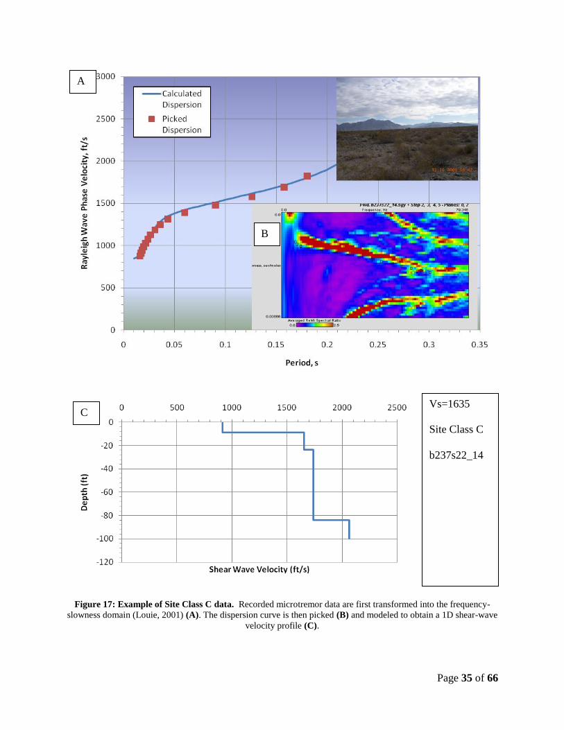
Figure 17: Example of Site Class C data. Recorded microtremor data are first transformed into the frequency-
slowness domain (Louie, 2001) (A). The dispersion curve is then picked (B) and modeled to obtain a 1D shear-wave
velocity profile (C).
Vs=1635
Site Class C
b237s22_14
C
B
A

Page 36 of 66
Figure 18: Example of Site Class C data. Recorded microtremor data are first transformed into the frequency-
slowness domain (Louie, 2001) (A). The dispersion curve is then picked (B) and modeled to obtain a 1D shear-wave
velocity profile (C).
Vs=1665
Site Class C
b216s06_24
C
B
A

Page 37 of 66
Figure 19: Example of Site Class D data. Recorded microtremor data are first transformed into the frequency-
slowness domain (Louie, 2001) (A). The dispersion curve is then picked (B) and modeled to obtain a 1D shear-wave
velocity profile (C).
Vs=1183
Site Class D
b031s34_36
C
B
A

Page 38 of 66
Figure 20: Example of Site Class D data. Recorded microtremor data are first transformed into the frequency-
slowness domain (Louie, 2001) (A). The dispersion curve is then picked (B) and modeled to obtain a 1D shear-wave
velocity profile (C).
Vs=734
Site Class D
b071s19_04
C
B
A

Page 39 of 66
Figure 21: Example of Site Class D data. Recorded microtremor data are first transformed into the frequency-
slowness domain (Louie, 2001) (A). The dispersion curve is then picked (B) and modeled to obtain a 1D shear-wave
velocity profile (C).
Vs=980
Site Class D
b223s22_21
C
B
A

Page 40 of 66
4.3 Shape of the dispersion curves
The shape of the dispersion curve varies due to the differing characteristics of the sub-surface
velocity structure. Figures 22 to 26 illustrate some of the typical variations observed.

Page 41 of 66
Figure 22: Example showing variation in the observed dispersion curve. Recorded microtremor data are first
transformed into the frequency-slowness domain (Louie, 2001) (A). The dispersion curve is then picked (B) and
modeled to obtain a 1D shear-wave velocity profile (C).
C
B
A
Vs=3193
Site Class B
b204s10_36

Page 42 of 66
Figure 23: Example showing variation in the observed dispersion curve. Recorded microtremor data are first
transformed into the frequency-slowness domain (Louie, 2001) (A). The dispersion curve is then picked (B) and
modeled to obtain a 1D shear-wave velocity profile (C).
Vs=1211
Site Class C
b264s23_20
C
B
A

Page 43 of 66
Figure 24: Example showing variation in the observed dispersion curve. Recorded microtremor data are first
transformed into the frequency-slowness domain (Louie, 2001) (A). The dispersion curve is then picked (B) and
modeled to obtain a 1D shear-wave velocity profile (C).
Vs=1018
Site Class D
b161s04_26
C
B
A

Page 44 of 66
Figure 25: Example showing variation in the observed dispersion curve. Recorded microtremor data are first
transformed into the frequency-slowness domain (Louie, 2001) (A). The dispersion curve is then picked (B) and
modeled to obtain a 1D shear-wave velocity profile (C).
Vs=1389
Site Class C
b223s01_18
C
B
A

Page 45 of 66
Figure 26: Example showing variation in the observed dispersion curve. Recorded microtremor data are first
transformed into the frequency-slowness domain (Louie, 2001) (A). The dispersion curve is then picked (B) and
modeled to obtain a 1D shear-wave velocity profile (C).
Vs=3127
Site Class B
b164s22_35
C
B
A

Page 46 of 66
4.4 Quality Assurance of the Results
Quality assurance of results begins by plotting of the velocity models within each section – (ca.
18 parcel measurements), as shown in Figure 27. Focus is accuracy of the average velocity
model in the upper 100 feet.
First check is to make sure the models are consistent within the section. Information from spatial
location, topographic, and geologic maps are utilized. If one model differs from surrounding
measurements, or is anomalous given known topographic changes, remodeling of the dispersion
curve picks is the first step. An alternate model which is more consistent may be able to be
derived. For some data sets, re-analysis of the original data may then occur. This may involve
adjustment of picks along indistinct dispersion curves or reconsideration of the curve itself.
Consistency of models with adjacent sections is also verified.
If there are anomalously high velocity layers within the upper 100 feet, the reliability of low
frequency dispersion curve picks is examined. In some cases, the accuracy of the dispersion
curves at low frequencies is unclear. Again, picks may be adjusted and the dispersion curve at
low frequencies is reconsidered.
If the site is classified as a Site Class B, the high frequency data is more carefully scrutinized to
ensure there is velocity information to determine layers in the upper 20 feet.

Page 47 of 66
Figure 27: Plot showing velocity versus depth plots for all arrays in b223s12 to a depth of 100 feet. The vertical red
line indicates a velocity of 2500 ft/s, while the horizontal red lines indicate depths of 10 ft and 20 ft. The values
along the top each model are the Vs100’, Vs20’ and Vs10’ values representing the average velocities calculated
using IBC equation 16-41 (Table 2) for the top 100’, 20’ and 10’
Page 48 of 66
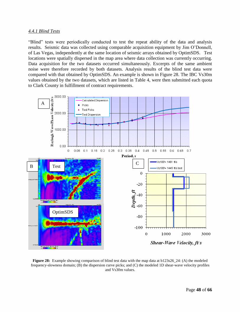
4.4.1 Blind Tests
“Blind” tests were periodically conducted to test the repeat ability of the data and analysis
results. Seismic data was collected using comparable acquisition equipment by Jim O’Donnell,
of Las Vegas, independently at the same location of seismic arrays obtained by OptimSDS. Test
locations were spatially dispersed in the map area where data collection was currently occurring.
Data acquisition for the two datasets occurred simultaneously. Excerpts of the same ambient
noise were therefore recorded by both datasets. Analysis results of the blind test data were
compared with that obtained by OptimSDS. An example is shown in Figure 28. The IBC Vs30m
values obtained by the two datasets, which are listed in Table 4, were then submitted each quota
to Clark County in fulfillment of contract requirements.
Figure 28: Example showing comparison of blind test data with the map data at b123s26_24: (A) the modeled
frequency-slowness domain; (B) the dispersion curve picks; and (C) the modeled 1D shear-wave velocity profiles
and Vs30m values.
A
B C
OptimSDS
Test

Page 49 of 66
Table4: List of Vs30m results from the map compared with those obtained through independent blind tests.
Quota 1 Vs Map (ft/s)
Vs Blind (ft/s)
Quota 2 Vs Map (ft/s)
Vs Blind (ft/s) Line
Line
1621803 1509 1524
1633620 3039 3128
1621921 1333 1353
1633621 3218 3296
1622202 1300 1364
1762118 3004 3101
1622633 1093 1096
1762132 3280 3273
1622932 1303 1417
1770114 950 940
1623121 1742 1783
1770119 1031 1016
1760335 3639 3410
1770808 1816 1917
1761325 2889 2898
1770830 2352 2201
Quota 3 Vs Map (ft/s)
Vs Blind (ft/s)
Quota 4 Vs Map (ft/s)
Vs Blind (ft/s) Line
Line
1610217 1274 1202
1400417 1203 1212
1610325 1319 1408
1400622 987 944
1630221 2560 2593
1401417 1920 1732
1630411 3317 3149
1401621 1117 1029
1630612 3408 3016
1401711 996 1007
1630914 3167 3516
1402305 2536 2464
1631005 3124 3234
1402320 2538 2577
1631105 2880 2990
1403534 1759 1694
Quota 5 Vs Map (ft/s)
Vs Blind (ft/s)
Quota 6 Vs Map (ft/s)
Vs Blind (ft/s) Line
Line
1250132 1047 1085
1611116 1493 1467
1250701 2997 3248
1611407 1094 1124
1252326 1102 1109
1613630 1454 1257
1252529 1396 1409
1640304 2476 2265
1252616 1282 1271
1640309 2123 2145
1253434 1123 1061
1640317 2394 2427
1253535 1282 1249
1751432 2732 3020
1253632 963 959
1751434 2823 2525
1751611 2671 2711
Quota 7 Vs Map (ft/s)
Vs Blind (ft/s)
Quota 8 Vs Map (ft/s)
Vs Blind (ft/s) Line
Line
1380729 2736 2816
1260210 2910 2964
1380809 2691 2853
1260604 2997 2898
1381325 1550 1437
1260733 2723 2740
1381519 2855 2953
1260911 2831 2871

Page 50 of 66
1381928 3101 3164
1261136 3028 3324
1382424 1298 1320
1261810 2646 2604
1382822 3191 3067
1262503 2732 2901
1383112 2648 2822
1262613 2847 2808
Quota 9 Vs Map (ft/s)
Vs Blind (ft/s)
Quota 11 Vs Map (ft/s)
Vs Blind (ft/s) Line
Line
2641306 1517 1680
0412622 1141 1208
2641508 1266 1270
0413424 715 732
2642431 1098 1067
0420225 2011 1953
2642834 1075 1051
0701330 1323 1295
0702411 1171 1200
Quota 10 Vs Map (ft/s)
Vs Blind (ft/s)
0713034 1415 1405
Line 2370801 1778 1761 2371608 1590 1608 2371619 1436 1543
Quota 12 Vs Map (ft/s)
Vs Blind (ft/s) Line
0090419 1483 1419 0091417 956 939 0091517 1325 1322 0092225 1402 1392 2160607 2166 2237 2160722 3039 2870 2171004 2568 2583 2171229 2166 2205 2172603 2210 2332 2230102 1683 1658 2230205 1402 1358 2230325 1368 1361 1232624 1461 1445 1232331 1554 1479 1220927 1391 1522

Page 51 of 66
4.5 Velocity Reversals
Caliche is distributed across much of the Las Vegas region. The high velocity caliche deposition
within subsurface layers can result in high velocity layers within the velocity-depth profile, with
lower velocity material below. These are referred to as velocity “reversals”. If reversals are
present in several models within a section, the depth of the inversion layer is attempted to be
fixed so that is occurs at the same depth throughout the surrounding area. The assumption is
made that the geology is not varying greatly over the short distances considered, and that the
caliche is developing in the same sedimentary layer within the section. Seismic lines
immediately adjacent to those with inversions may be modeled with an inversion layer even if
they can be modeled without an inversion, based on this assumption. Examples of data with
inversions are given in Figures 29 to 32.
In some cases, to maintain constant bedrock velocities within a section with topographic highs,
small reversals may be introduced into the model (Figures 33 and 34).

Page 52 of 66
Figure 29: Example of Site Class D data that produced model with velocity reversal a depth. Recorded microtremor
data are first transformed into the frequency-slowness domain (Louie, 2001) (A). The dispersion curve is then
picked (B) and modeled to obtain a 1D shear-wave velocity profile (C).
Vs=1178
Site Class D
b138s01_13
C
B
A

Page 53 of 66
Figure 30: Example of Site Class B data that produced model with velocity reversal a depth. Recorded microtremor
data are first transformed into the frequency-slowness domain (Louie, 2001) (A). The dispersion curve is then
picked (B) and modeled to obtain a 1D shear-wave velocity profile (C)
Vs=2527
Site Class B
b204s20_27
C
B
A

Page 54 of 66
Figure 31: Example of Site Class C data that produced model with velocity reversal a depth. Recorded microtremor
data are first transformed into the frequency-slowness domain (Louie, 2001) (A). The dispersion curve is then
picked (B) and modeled to obtain a 1D shear-wave velocity profile (C).
Vs=1262
Site Class C
b264s22_07
C
B
A

Page 55 of 66
Figure 32: Example of Site Class D data that produced model with velocity reversal a depth. Recorded microtremor
data are first transformed into the frequency-slowness domain (Louie, 2001) (A). The dispersion curve is then
picked (B) and modeled to obtain a 1D shear-wave velocity profile (C).
Vs=1182
Site Class D
b161s20_15a
C
B
A

Page 56 of 66
Figure 33: Small inversions are introduced into the model so as to maintain constant bedrock velocities within a
section with topographic highs. Example for a Site Class C site.
Vs=1205
Site Class C
b264s28_21
C
B
A

Page 57 of 66
Figure 34: Small inversions are introduced into the model so as to maintain constant bedrock velocities within a
section with topographic highs. Example for a Site Class D site.
Vs=1188
Site Class D
b264s33_10
C
B
A

Page 58 of 66
5.0 Results: Microzonation Map
As part of the project, data from a total of 9006 sites were acquired, processed and submitted to
the City. This represents 100% of the total number of seismic array lines (~9000) scheduled to be
collected as part of this project. Figure 35 depict these seismic array locations across Clark
County. More detailed maps in Figure 36 display the Las Vegas Valley (Figure 36(a)), the I15
southern corridor including Jean and Primm (Figure 36(b)), Coyote Springs (Figure 36(c),
Moapa Valley, Longdale, and Overton (Figure 36(d)), and Laughlin (Figure 36(e)).
Appendix A (on DVD) shows the microzonation map generated using ArcGIS and the Vs100’
values determined from the distribution of seismic arrays in Clark County. The method of
krigging was used to produce this map. The microzonation map has been produced in a format
(digitally delivered to Clark County) so it can be easily integrated into Clark County’s present
internet based public information system. The map for the City of Henderson was completed in
tandem with the Clark County microzonation project. As such, the map that is produced took
into account the microzonation values obtained in the adjoining City of Henderson areas.
Appendix B (on DVD) shows the one-dimensional (1D) shear wave (Vs) velocity models at
seismic array locations, and the IBC Site Class and Vs100’ (or Vs30m) calculated from these
profiles down to 100 feet using IBC equation 16-41 (Table 2). It is to be noted that additional
criteria as listed in Table 3 must be used when Site Class B is encountered. Site specific
determination by a professional engineer might be required to make sure it can be classified as a
Site Class B site.
Appendix C (on DVD) GIS referenced shapefile map showing the Vs100’, Vs20’ and Vs10’
values representing the average velocities calculated using IBC equation 16-41 (Table 2) for the
top 100’, 20’ and 10’ for all Clark County seismic array lines.
Appendix D: List of seismic arrays for which geometry information was collected.

Page 59 of 66
Figure 35: Clark County and the surrounding valleys with all seismic array lines to date. Lines shown in green were
part of the contract areas for the City of Henderson. Red boxed areas outline the regions shown in Figures 36(a) to
36(e).
Figure 36(a): Las Vegas Valley with all seismic array lines to date. Lines shown in green were part of the contract
areas for the City of Henderson.

Page 60 of 66
Figure 36(b): The I15 southern corridor including Jean and Primm with all seismic array lines to date. Lines shown
in green were part of the contract areas for the City of Henderson.
Figure 36(c): Coyote Springs with all seismic array lines to date.

Page 61 of 66
Figure 36(d): Moapa Valley, Longdale, and Overton with all seismic array lines to date.
Figure36(e): Laughlin with all seismic array lines to date.
Page 62 of 66
6.0 Other Deliverables
In addition to the maps and one dimensional model shown in the Appendices, the following were
posted on Optim SDS secure FTP site for Clark County personnel to download:
GIS referenced shapefile map showing the 100’ average velocities as per IBC 2006
section 1613.5.5. This can be imported into ArcGIS to plot and visualize the values
(Appendix C, on DVD).
Text files showing the velocity profile down to 100 feet and the IBC value.
Associated slowness-frequency image with Rayleigh-wave dispersion curve picks.
ARC color map showing the 100’ velocities color coded as per IBC
Access to the FTP site has been provided to Clark County personnel.
7.0 Conclusions and Recommendations
The project was completed successfully for Clark County. The Nevada System of Higher
Education (NSHE) via the subcontractor Optim Seismic Data Solutions measured shallow shear-
velocity velocities throughout the approximately 500 square miles of Clark County. This project
was conducted in conjunction with City of Henderson Building Department with the objective of
creating a complete map for the Valley. In all, 9006 individual seismic arrays/lines were
assigned, deployed and spatially located using Geographical Positioning System (GPS) in a
systematic manner in order to maximize the data density coverage of the database within Clark
County.
It is recommended that Clark County personnel use other resources at their disposal to per
determine the form the microzonation map should be disseminated to the public. For example, it
is recommended that overlaying the land parcel layer would provide valuable information on
how to classify parcels as per the microzonation (Site Class) map. If the microzonation map
overlay shows two different site class for the same parcel, it is recommended the more
conservative value be used as the default site class for that parcel. It is also to be noted that Site
Class B values in the microzonation map shown in Appendix C is based purely on the Vs100’
value. IBC 2006 Section 1613.5.5 states that: The rock categories, Site Classes A and B, shall
not be used if there is more than 10 feet (3048 mm) of soil between the rock surface and the
bottom of the spread footing or mat foundation. So, when the values suggest a B, site specific
consideration should be made (depth of foundation, competency of rock etc) before deciding
whether it is a Site Class B.
8.0 References
Building Seismic Safety Council, BSSC, 1997, NEHRP Recommended Provisions for Seismic
Regulations for New Buildings and other Structures, Part1 – Provisions, Federal Emergency
Management Agency, Washington D.C., and FEMA 302.
International Building Code, 2006, International Code Council, pages 679.

Page 63 of 66
Iwata, T., Kawase, H., Satoh, T., Kakehi, Y., Irikura, K., Louie, J. N., Abbott, R. E., and
Anderson, J. G., 1998, Array microtremor measurements at Reno, Nevada, USA (abstract):
Eos, Trans. Amer. Geophysical. Union, v. 79, suppl. to no. 45, p. F578.
Louie, J, N., 2001, Faster, Better: Shear-wave velocity to 100 meters depth from refraction
microtremor arrays: Bulletin of the Seismological Society of America, v. 91, p. 347-364.
Saito, M., 1979, Computations of reflectivity and surface wave dispersion curves for layered
media; I, Sound wave and SH wave: Butsuri-Tanko, v. 32, no. 5, p. 15-26.
Saito, M., 1988, Compound matrix method for the calculation of spheroidal oscillation of the
Earth: Seismol. Res. Lett., v. 59, p. 29.
Stephenson, W. J., J. N. Louie, S. Pullammanappallil, R. A. Williams, and J. K. Odum, (2005).
Blind shear-wave velocity comparison of ReMi and MASW results with boreholes to 200 m
in Santa Clara Valley: Implications for earthquake ground motion assessment, Bulletin of the
Seismological Society of America, 95, 2506-2516, doi: 10.1785/0120040240.
Thelen, W. A., M. Clark, C. T. Lopez, C. Loughner, H. Park, J. B. Scott, S. B. Smith, B.
Greschke, and J. N. Louie (2006). A transect of 200 shallow shear-velocity profiles across the
Los Angeles basin, Bulletin of the Seismological Society of America, 96, 1055-1067.
Xia, J., Miller, R. D., and Park, C. B., 1999, Estimation of near-surface shear-wave velocity by
inversion of Rayleigh wave: Geophysics, v. 64, p. 691-700.

Page 64 of 66
Appendix D: List of seismic arrays for which geometry information was collected.
0090420 0313421 0412107 0412108 0412110a 0412110b 0412116 0412122
0412126 0412127 0420302 0420307 0420315 0702402 0713023 1220201 1220206 1220212 1220332
1220421 1220916 1220922 1221023 1221025 1221101
1221104 1221105 1221107 1221111 1221123
1221505 1221516 1221602 1221610 1221622 1222010 1222101 1222214 1222234
1222236 1222310 1222332 1250201 1250426 1251001 1251006 1251009
1251010 1251011 1251012 1251018 1251021 1251026 1253408 1253409 1253422 1253426 1253612
1253613 1253616 1253627 1253628 1260306 1260328
1260412 1260426 1260812 1260830 1260904
1261001 1261009 1261207 1261219 1261229 1261230 1261307 1261311 1261314
1261403 1261415 1261801 1262210 1262228 1262234 1262703 1262717
1262735 1263410 1263417 1263419 1263420 1263427 1263428 1263429 1263435 1263502 1263518
1263521 1263523 1263527 1263531 1263533 1263632
1263636 1380107 1380110 1380111 1380116
1380619 1380620 1380714 1380722 1381605 1381614 1381616 1381617 1381631
1381633 1381634 1381706 1381708 1381729 1381732 1381733 1381814
1381819 1381824 1381826 1381828 1381906 1381910 1381916 1381917 1381926 1381936 1382003
1382007 1382010 1382016 1382022 1382027 1382030
1382031 1382035 1382107 1382108 1382115
1382116 1382118 1382121 1382129 1382131 1382133 1382136 1382312 1382511

Page 65 of 66
1382528 1382601 1382604 1382611 1382702 1382805 1382813 1382814 1382908 1382920 1382931
1383002 1383011 1383012 1383013 1383020 1383024 1383025 1383026 1383027 1383031 1383033
1383107 1383113 1383116 1383119 1383215 1383217 1383226 1383333 1383336
1383610 1383622 1401534
1402210 1402334 1402335 1402424 1402425 1402601 1402609 1402613 1402626
1402811 1403503 1403511 1403514 1403523 1403526 1403535 1601917 1601925 1602801 1602902
1602904 1602908 1602912 1602922 1602927 1603022 1603026 1610105 1610107 1610109 1610121
1610129 1610130 1610133 1610134 1610426 1610429b 1610909 1611233 1611313
1611315 1611328 1611435
1611523a 1611525 1611636 1611712a 1611814a 1611915 1612127a 1612231a 1612412
1612515 1612523 1612826 1613023a 1613406a 1621020 1621022 1621023 1621028 1621220 1621616
1621627 1621703 1621704 1621713 1622002 1622006 1622010 1622034 1622207 1630526 1630816
1630821 1632208 1632711 1632808 1633129 1640111 1640131 1640208 1640216
1640219 1640226 1640306
1640307 1640401 1640410 1640411 1641102 1641104 1641106 1641108 1641131
1641133 1641207 1641211 1641219 1641229 1641235 1641315 1641404 1641405 1641409 1641411
1641414 1641415 1641417 1641420 1641422 1641424 1641425 1641427 1641429 1641431 1641432
1642214 1642223 1642231 1642302 1642308 1642311 1642316 1642318 1642321
1642323 1642325 1642328
1642333 1642405 1642407 1642409 1642413 1642416 1642424 1642427 1642429

Page 66 of 66
1642430 1642435 1642509 1642510 1642519 1642520 1642525 1642529 1643601 1643604 1643611
1643623 1643635 1751301 1751305 1751309 1751311 1751404 1751407 1751420 1751432 1751501
1751512 1751523 1751524 1751526 1751534 1751607 1751609 1751621 1751626
1751633 1752405 1752406
1752410 1760632 1761022 1762026 1763104 1763231 1763234 1763535 1770234
1770330 1771123 1771125 1771316a 1773619 1773634 1910521 1910602 1910611 1910615 1910617
1910618 1910619 1910620 1910621 1910633 1910636 1910718 1910720 1910728 1910734 1911710
1911802 1911810 1911812 1920210 1922401 1923608 1923610 1923614 1923616
1923621 1923629 2040106
2040110 2040213 2040235 2041001 2041013 2041020 2041026 2041112 2041202
2041234 2041415 2041416 2041421 2041623 2043002 2043126 2043219 2160511 2160519 2160612
2160624 2160706 2160719 2160728 2160729 2160818 2160819 2163011 2163023 2171224 2172531
2173605 2173606 2173614 2173618 2231315 2232931 2370814 2640116 2640131
2640226 2641018 2641126
2641307 2641512 2642108 2642132 2642225 2642231 2642308 2642320 2642419
2642505 2642517 2642607 2642621 2642622 2642702 2642714 2642718 2642722 2642730