large databases and performance lecture uio 31. oct. 2011 ... · accenture technology consulting...
TRANSCRIPT

Accenture Technology Consulting
Large databases and performance
Lecture UiO 31. oct. 2011
Audun Faaberg - Accenture

2 Copyright © 2011 Accenture All Rights Reserved.
Agenda
1. Introduction.
2. Tune the SW (reduce the IO)
a. Indices
b. Efficient SQL
c. Efficient code & design
3. SOA, object orientation, distance
4. Performance engineering
5. Real life examples

3
About me • Senior manager in Accenture Technology Consulting, leading the Performance
engineering group in Norway & the Nordics.
• Worked in Arthur Andersen / Andersen Consulting / Accenture since 1989.
• Specialise in technical project management in large multi platform environments.
• Key words are operating systems, data base technology, performance, conversions, go-live, problem management and supplier management.
• DB2, Oracle, MSSQL, Unix, ZOS, Cobol, C, Java, Tuxedo, MQ, CICS, WebLogic, WebSphere, MIIS ++
• In free time, enjoy mountains, skiing, I am a certified glacier guide…..
Copyright © 2011 Accenture All Rights Reserved.

4
About Accenture
• 236.000 employees, worldwide (31. Aug 2011).
• Largest country: India.
• 1100 employees, Norway.
• Offices in Oslo, Bergen, Stavanger.
• In the Nordics – Helsinki, Stockholm, Gothenburg, Copenhagen, + nearshore centre in Riga.
• Many of the largest companies in each country are clients.
• Currently in Norway, 30% of our work is in public sector.
Copyright © 2011 Accenture All Rights Reserved.
5
Disclaimer :-)
• I have worked in Norway, Denmark, France, Italy,
Brazil, The Czech Republic, Malaysia – MEANING –
“a telco” is not Telenor, “a bank” is not DnB NOR,
“an oil company” is not StatoilHydro……
• Specific numbers may be old (page size, cache size,
IO speed). But the logic should still apply, though of
course the massive changes currently may lead to
this logic producing another result…..
• This is not a full course of tuning in large databases,
it is to make you aware of what is there…
Copyright © 2011 Accenture All Rights Reserved.

6
1. Introduction
Basic arithmetic
0.000 sec x 6,000,000 = 0 sec
0.012 sec x 6,000,000 = 72000 sec = 20 hours
Many designers think this is the database speed
And this may be the real database
speed
Copyright © 2011 Accenture All Rights Reserved.

7
1. Introduction
Poor performance
• Poor performance in the database and the code using the
database is the most common reason for poor system
performance.
• Poor performance may render an otherwise good system
useless. Or despised. Or lead to ineffective organisations
and numerous coffee breaks….
• Problems with performance may cause large delays in the
final phases of a project, though should be more
manageable than other issues that may occur at this stage.
• Finally, there is a lack of understanding that optimising
code may drastically alter CPU &IO consumption.
Therefore, more HW is the normal (often wrong) answer.
Copyright © 2011 Accenture All Rights Reserved.

8
1. Introduction
Why is there still a problem
• HW is faster. CPU, disks, network, memory, everything is much faster now than 10 years ago.
• Moore‟s law: Integrated circuits would double in performance every 18 months
• Why is there still a problem?
• Niklaus Wirth‟s law: Software is s getting slower more rapidly than hardware becomes faster
• To be more specific – Gate‟s law: The speed of commercial software generally slows by fifty percent every 18 months
Copyright © 2011 Accenture All Rights Reserved.

9
1. Introduction
Why is there still a problem
• Databases are now more finely modelled, catching more data, and creating complexities an order of magnitude greater.
• Flexible, parameterised, configurable system use many small parameter tables, which are used in every select. So earlier when a select referenced 2-3 tables, it may now reference 8-10 tables to fetch the same data. (And beware if a system is “generic”)
• Much larger ambitions – meaning – now much larger data volumes are stored. 10-15 years ago, we were stingy when designing databases.
• And – even if CPUs double their speed every 18 month, disk IO speed has only increased 10-100 x since the 1960s.
• Shift to client – server – and now network computing: Adds network latency, integration with other systems, much larger data volumes, more complex user interfaces, more complex processes and a large degree of aggregation of information.
Copyright © 2011 Accenture All Rights Reserved.

10
1. Introduction
Example of data modelling
Loan
Cust_id Balance
10 2,405,256
20 1,530,203
Loan
Cust_id Loan-_series_id
10 1,562,030
20 1,830,203
Loan_series (one record for every month throughout 20 years)
Loan_series_id Year Month Org_amount Remaining Interests
1,562,030 2008 01 2,405,256 2,395,256 23,952
1,562,030 2008 02 2,405,256 2,375,256 23,752
… … … … …
1,562,030 2028 12 2,405,256 20,000 200
Earlier modelling, 1 record pr loan
2 million
customers
2 million rows
482 million rows
Recent modelling, 241 records pr
loan
Functionally more flexible, but at a cost
Copyright © 2011 Accenture All Rights Reserved.

11
2. Tune the SW
Note: Tuning of SQL is typically a 40 hours introduction
course + 5 years experience.
This is just a broad overview, so you will know there is more
(much more) to know.
– Indices
– Efficient SQL
– Efficient code & design
Basic principles
- Divide and conquer
- Minimise the fetch of everything
Copyright © 2011 Accenture All Rights Reserved.

12
2. Tune the SW
Another view
Poor SQL = HIGH IO and CPU
load to execute Your SQL code 10.000 page IO 1000 users 10 mill IO pr min
Your SQL code 15 page IO 1000 users 15.000 IO pr min
Ridiculously expensive
disk system
Inexpensive disk system
Clever SQL = Low IO and CPU load to exectute
Copyright © 2011 Accenture All Rights Reserved.

13
2. Tune the SW
A DBMS model
Page
4 KB
max 255
rows
(15 byte)
Disks
Though, 150 bytes pr record
=> 26 rows pr page
Network Track
Typical IO time: 10 ms for a page read
NOTE: Page size Oracle 0,5-64K.
Best: Match file system. Minimum 4
data rows. The larger the better, though
concurrency may dictate otherwise Copyright © 2011 Accenture All Rights Reserved.
Internal memory (1-2-4-8-16 GB?)
2 GB => 0,5 mill pagers CPU
Fig
ure
: Au
du
n F
aab
erg
Reader head

Copyright © 2008 Accenture All Rights Reserved. 14
2. Tune the SW – a. indices
What are indices – real world example
Fig
ure
: Jan
Hau
gla
nd
• Oslo Map
– Map pages
– Index pages
• Index
– Carl Berners Plass 16 G3
– Tullinløkka 10 F2

15
2. Tune the SW – a. indices
What are indices
190K3
190K2
620K1
68270K3
79040K2
21100K1
21299K3
08529K2
43332K1
24701K3
53701K2
98776K1
38270K3
43310K2
00000K1
10297K3
00544K2
11000K1
06242K3
97630K2
11111K1
377K3
YXADATA
441K2
000K1
220K3
CXBDATA
030K2
100K1
089K3
BYADATA
034K2
100K1
162K3
CYADATA
075K2
110K1
204K3
CYADATA
693K2
111K1
......
......
Data pages
Index leaf pages
Index pages
Fig
ure
: Jan
Hau
gla
nd
Copyright © 2011 Accenture All Rights Reserved.
16
2. Tune the SW – a. indices
What are indices
• A tree downwards through index pages, and on the leaf pages there is a pointer to the very page and an offset for the row in question.
• The indices are stored in index spaces (corresponding to table spaces)
• The disk space used by the index spaces may be as large as for the table spaces.
• Since the columns of an index is (normally) fewer than in the complete row, more are stored in a page (though max 255). Thus a index scan is faster than a table scan.
• May dramatically lower the number of pages read to find a row. Read through 3-4 layers of indices (pages), versus scanning the whole table with thousands of pages.
Copyright © 2011 Accenture All Rights Reserved.

17
2. Tune the SW – a. indices
Full Table Scan
SELECT K2
FROM SIMPLE_TABLE
WHERE DATA = ‘X’
• All yellow keys match
• All blue values returned
• All red pages scanned
190K3
190K2
620K1
68270K3
79040K2
21100K1
21299K3
08529K2
43332K1
24701K3
53701K2
98776K1
38270K3
43310K2
00000K1
10297K3
00544K2
11000K1
06242K3
97630K2
11111K1
377K3
YXADATA
441K2
000K1
220K3
CXBDATA
030K2
100K1
089K3
BYADATA
034K2
100K1
162K3
CYADATA
075K2
110K1
204K3
CYADATA
693K2
111K1
......
......
Data pages
Index leaf pages
Index pages
• Let us assume the table
has 50 mill rows, 20
rows pr page. (page 4K,
row 200 bytes).
• In mean 1.250.000 page
reads to find a random
row.
• 10 ms pr page read…..
12.500 sec = 3,5 hours
Fig
ure
: Jan
Hau
gla
nd
Copyright © 2011 Accenture All Rights Reserved.

18
2. Tune the SW – a. indices
Non-matching Index Scan
SELECT DATA
FROM SIMPLE_TABLE
WHERE K3 = 7
• All yellow keys match
• All blue values returned
• All red pages scanned
• Let us assume the table
has 50 mill rows, 20
rows pr page.
• Indices: 20 bytes – 200
on each page. 250.000
leaf pages
• 125.000 IOs -> 1250 s.
190K3
190K2
620K1
68270K3
79040K2
21100K1
21299K3
08529K2
43332K1
24701K3
53701K2
98776K1
38270K3
43310K2
00000K1
10297K3
00544K2
11000K1
06242K3
97630K2
11111K1
377K3
YXADATA
441K2
000K1
220K3
CXBDATA
030K2
100K1
089K3
BYADATA
034K2
100K1
162K3
CYADATA
075K2
110K1
204K3
CYADATA
693K2
111K1
......
......
Data pages
Index leaf pages
Index pages
Fig
ure
: Jan
Hau
gla
nd
Copyright © 2011 Accenture All Rights Reserved.

19
2. Tune the SW – a. indices
Specify your select
SELECT K2, K3
FROM SIMPLE_TABLE
WHERE K3 = 7
• Will result in a scan of
the index leaf pages
• No read of data pages
necessary.
• This is one reason to
avoid SELECT * and
rather specify the
columns.
190K3
190K2
620K1
68270K3
79040K2
21100K1
21299K3
08529K2
43332K1
24701K3
53701K2
98776K1
38270K3
43310K2
00000K1
10297K3
00544K2
11000K1
06242K3
97630K2
11111K1
377K3
YXADATA
441K2
000K1
220K3
CXBDATA
030K2
100K1
089K3
BYADATA
034K2
100K1
162K3
CYADATA
075K2
110K1
204K3
CYADATA
693K2
111K1
......
......
Data pages
Index leaf pages
Index pages
Fig
ure
: Jan
Hau
gla
nd
Copyright © 2011 Accenture All Rights Reserved.

20
2. Tune the SW – a. indices
Matching Index Scan
SELECT DATA
FROM SIMPLE_TABLE
WHERE K1 = 0
AND K2 = 3
• All green keys match
• All yellow index entries
used
• All blue values returned
• All red pages scanned
• Let us assume the table
has 50 mill rows, 20
rows pr page.
• Indeces: 20 bytes – 200
on each page. 250.000
leaf pages, need 3 levels
of index pages.
• 5 IOs -> 50 ms.
Fig
ure
: Jan
Hau
gla
nd
0
0
0
7
4
0
1 9 0 K3
1 9 0 K2
6 2 0 K1
6 8 2 K3
7 9 0 K2
2 1 1 K1
2 1 2 9 9 K3
0 8 5 2 9 K2
4 3 3 3 2 K1
2 4 7 0 1 K3
5 3 7 0 1 K2
9 8 7 7 6 K1
3 8 2 7 0 K3
4 3 3 1 0 K2
0 0 0 0 0 K1
1 0 2 9 7 K3
0 0 5 4 4 K2
1 1 0 0 0 K1
0 6 2 4 2 K3
9 7 6 3 0 K2
1 1 1 1 1 K1
3 7 7 K3
Y X A DATA
4 4 1 K2
0 0 0 K1
2 2 0 K3
C X B DATA
0 3 0 K2
1 0 0 K1
0 8 9 K3
B Y A DATA
0 3 4 K2
1 0 0 K1
1 6 2 K3
C Y A DATA
0 7 5 K2
1 1 0 K1
2 0 4 K3
C Y A DATA
6 9 3 K2
1 1 1 K1
......
......
Data pages
Index leaf pages
Index pages
Copyright © 2011 Accenture All Rights Reserved.

21
2. Tune the SW – a. indices
Sequential prefetch
• A correction – the table scans are in fact
more efficient than depicted in the earlier
examples.
• A mechanism “Sequential prefetch” (or
“scatter read”) is invoked when the DBMS
discovers that it is reading in sequence
through the pages (typically 3 in sequence
within 10 reads).
190K3
190K2
620K1
68270K3
79040K2
21100K1
21299K3
08529K2
43332K1
24701K3
53701K2
98776K1
38270K3
43310K2
00000K1
10297K3
00544K2
11000K1
06242K3
97630K2
11111K1
377K3
YXADATA
441K2
000K1
220K3
CXBDATA
030K2
100K1
089K3
BYADATA
034K2
100K1
162K3
CYADATA
075K2
110K1
204K3
CYADATA
693K2
111K1
......
......
Data pages
Index leaf pages
Index pages
• Starts to read 50 and 50 pages, typically at 30 ms (compared to 10 ms for one
page). Leading to 25.000 read operations in a full table scan, or 750 / 2 sec =
6,25 minutes to find a random row (mean).
• Also the non-matching index scan will start prefetching. Leading to 4.000
read operations, or 120 / 2 sec = 60 sec.
• This can be utilised in large batch reads!
• Typically – if you try to select more than 10% of the rows in a table, the
optimiser will go for a table scan.
Fig
ure
: Jan
Hau
gla
nd
Copyright © 2011 Accenture All Rights Reserved.
22
2. Tune the SW – a. indices
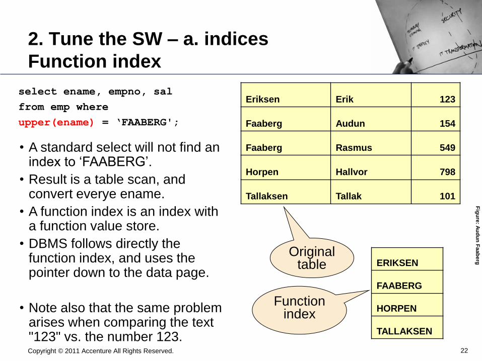
Function index
select ename, empno, sal
from emp where
upper(ename) = ‘FAABERG';
Eriksen Erik 123
Faaberg Audun 154
Faaberg Rasmus 549
Horpen Hallvor 798
Tallaksen Tallak 101
ERIKSEN
FAABERG
HORPEN
TALLAKSEN
• A standard select will not find an index to „FAABERG‟.
• Result is a table scan, and convert everye ename.
• A function index is an index with a function value store.
• DBMS follows directly the function index, and uses the pointer down to the data page.
• Note also that the same problem arises when comparing the text "123" vs. the number 123.
Original table
Function index
Fig
ure
: Au
du
n F
aab
erg
Copyright © 2011 Accenture All Rights Reserved.

23
2. Tune the SW – b. efficient SQL
Optimiser
Disks
Statistics
• Note: The optimiser is just a machine (or more correct
– another piece of software) doing the best it can.
• It may err – and with disastrous results.
• A DBA I know – after several hours of testing different
setups: “Finally I framed the optimiser!”
• Cost based optimiser:
Uses statistics, and
weighs operations.
Copyright © 2011 Accenture All Rights Reserved.
Network
Fig
ure
: Au
du
n F
aab
erg
Reader head
Internminne (1-2-4-8-16 GB?)
2 GB => 0,5 mill pager CPU
Optimiser

24
2. Tune the SW – b. efficient SQL
Access path
• Access path is the way and sequence the DBMS applies
rules. Using an index? Joins – in which order? Sort?
• It may be necessary to understand the access path.
• A database simulator tool may help you.
• In large projects with large database – we sometimes have
a centralised function approving all SQL (typically testing in
with the simulator… or on a large test database).
• You set up the simulator with the estimated number of rows
in the different tables, indicates a cardinality / distribution
(meaning – for large projects this is no small effort!)
Copyright © 2011 Accenture All Rights Reserved.

25
2. Tune the SW – b. efficient SQL
Looking for the millionaire
Before we start looking at SQLs and access paths - let us look at the real
word. Tax is fun.
How would you find the millionaires in Modalen county (one of the
smallest counties in Norway). By hand, by sifting through index cards.
a) Give me index cards of the millionaires in Norway, with the county
added on. Read through the index cards.
b) Give me all index cards of Modalen. I will scan through all of it.
And for Oslo?
t_adresse
Modalen
t_person t_loenn
Pnr = 070777 32678
Pnr = 080888 31293
Loenn = 469 000
Loenn = 1 296 059
Distribution info Modalen: 274 taxpayers Oslo: 439 272 taxpayers Over 1 mill in Norway: 60 261
Oslo
Copyright © 2011 Accenture All Rights Reserved.

26
2. Tune the SW – b. efficient SQL
Access path
Consider the employee table
With no function index:
With an function index on upper(ename):
select ename, empno, sal
from emp where
upper (ename) = ‘FAABERG';
Eriksen Erik 123
Faaberg Audun 154
Faaberg Rasmus 549
Horpen Hallvor 798
Tallaksen Tallak 101 0 SELECT STATEMENT Optimizer=COST
1 0 TABLE ACCESS (FULL) OF ‘EMPLOYEE_TABLE‘ 50
0 SELECT STATEMENT Optimizer=CHOOSE
1 0 INDEX (RANGE SCAN) OF ‘UPPER_ENAME_IDX' (NON-UNIQUE) 1
Copyright © 2011 Accenture All Rights Reserved.
27
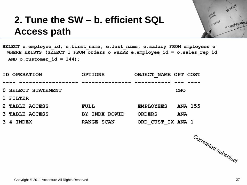
2. Tune the SW – b. efficient SQL
Access path
SELECT e.employee_id, e.first_name, e.last_name, e.salary FROM employees e
WHERE EXISTS (SELECT 1 FROM orders o WHERE e.employee_id = o.sales_rep_id
AND o.customer_id = 144);
ID OPERATION OPTIONS OBJECT_NAME OPT COST
---- ------------------ --------------- ----------- --- ----
0 SELECT STATEMENT CHO
1 FILTER
2 TABLE ACCESS FULL EMPLOYEES ANA 155
3 TABLE ACCESS BY INDX ROWID ORDERS ANA
3 4 INDEX RANGE SCAN ORD_CUST_IX ANA 1
Copyright © 2011 Accenture All Rights Reserved.

28 Copyright © 2008 Accenture All Rights Reserved.
2. Tune the SW – b. efficient SQL
Access path
SELECT e.employee_id, e.first_name, e.last_name, e.salary
FROM employees e
WHERE e.employee_id IN
(SELECT o.sales_rep_id
FROM orders o WHERE o.customer_id = 144);
ID OPERATION OPTIONS OBJECT_NAME OPT COST
---- ------------------ --------------- ----------- --- ----
0 SELECT STATEMENT CHO
1 NESTED LOOPS 5
2 VIEW 3
3 SORT UNIQUE 3
4 TABLE ACCESS FULL ORDERS ANA 1
5 TABLE ACCESS BY INDEX ROWID EMPLOYEES ANA 1
6 INDEX UNIQUE SCAN EMP_ID_PK ANA 1
A rewrite of the SQL

29 Copyright © 2008 Accenture All Rights Reserved.
2. Tune the SW – b. efficient SQL
Inner Join
T_KRAVHODE
KRAVHODE_ID SAK_ID
10 100
20 200
T_KRAVLINJE
KRAVHODE_ID KRAVLINJE_ID
20 2000
30 3000
QUERY RESULT
SAK_ID KRAVLINJE_ID
200 2000
SELECT H.SAK_ID
,L.KRAVLINJE_ID
FROM T_KRAVHODE H
,T_KRAVLINJE L
WHERE L.KRAVHODE_ID = H.KRAVHODE_ID
Equivalent to:
SELECT H.SAK_ID
,L.KRAVLINJE_ID
FROM T_KRAVHODE H
INNER JOIN
T_KRAVLINJE L
ON L.KRAVHODE_ID = H.KRAVHODE_ID
Copyright © 2011 Accenture All Rights Reserved.

30 Copyright © 2008 Accenture All Rights Reserved.
2. Tune the SW – b. efficient SQL
Missing join predicate
T_KRAVHODE
KRAVHODE_ID SAK_ID
10 100
20 200
T_KRAVLINJE
KRAVHODE_ID KRAVLINJE_ID
20 2000
30 3000
QUERY RESULT
SAK_ID KRAVLINJE_ID
100 2000
100 3000
200 2000
200 3000
SELECT H.SAK_ID
,L.KRAVLINJE_ID
FROM T_KRAVHODE H
,T_KRAVLINJE L
This is the infamous
Carthesian product
A X B ={ (a,b)| a Є A A b Є B }
Copyright © 2011 Accenture All Rights Reserved.

31 Copyright © 2008 Accenture All Rights Reserved.
2. Tune the SW – b. efficient SQL
Why are carthesians disastrous?
Person
Person_number Name
05056847126 Hans Alnes
09118910017 Kari Thune
Account
Person_number Account_number
05056847126 1533 289 08971
05056847126 1533 289 08988
05056847126 In mean 5 accounts
09118910017 1540 780 01122
09118910017 9833 010 89876
09118910017 In mean 5 accounts
SELECT P.Person_number
,A.Bank_account
FROM T_Person P
,T_Account A
4,5 million
persons
22,5 million
accounts
SELECT P.Person_number
,A.Bank_account
FROM T_Person P
,T_Account A
WHERE P.Person_number = A.Person_number
Here Hans Alnes is matched with ALL accounts in
Norway (22,5 millions of them)
Thereafter Kari Thune is matched with ALL accounts
Giving a list of 4,5 * 22,5 million² = 101,25 mill mill
101 250 000 000 000 items
25 million seconds (seq prefetch)
Here Hans Alnes is matched with his 5 accounts
Thereafter Kari Thune is matched with her 5 accounts
Giving a list of 4,5 million * 5 = 22,5 mill
(30-40 seconds with seq prefetch)

32 Copyright © 2008 Accenture All Rights Reserved.
2. Tune the SW – b. efficient SQL
Correlated subselect
• A subselect is correlated if it has reference to column values in the outer select.
• OK as filtering refinement. Extremely expensive as main filtering!
• Example: select h.kravhode_id
from t_kravhode h
where h.sak_id = ?
and exists
(select 1
from t_kravlinje l
,t_kravlinje_s s
where l.kravhode_id = h.kravhode_id
and s.kravlinje_id = l.kravlinje_id
and s.k_kravlinje_s = ?)
t_kravhode
sak_id = 97864 kravhode = 6887 1 line returned = good filtering in main select
t_kravlinje t_kravlinje_s (status)
kravhode = 6887 kravlinje_id = 5
kravhode = 6887 kravlinje_id = 6
kravlinje_id = 5 kravlinje_s =”A”
kravlinje_id = 6 kravlinje_s =”A”
Must go to these two tables for every row in t_kravhode which qualifies But the outer select is a good filter

33 Copyright © 2008 Accenture All Rights Reserved.
2. Tune the SW – b. efficient SQL
Non-correlated subselect
•A subselect is non-correlated if it has no reference to column values in the outer select. •OK as main filtering. Extremely expensive as filtering refinement! Example: select s.sak_id
,s.dato_endret
from t_sak s
where s.sak_id = in
(select h.sak_id
from t_kravhode h
,t_kravlinje l
where h.kravhode_id = l.kravhode_id
and l.person_id = ?)
t_kravhode
sak_id = 97864 kravhode = 6887
t_kravlinje t_sak
kravhode = 6887 person_id = 1030
kravhode = 7356 person_id = 1030
kravlinje_id = 5 kravlinje_s =”A”
kravlinje_id = 6 kravlinje_s =”A”
The select starts here, set up a small number of columns which qualify for the OUTER select
sak_id = 57891 kravhode = 7356
2 lines returned = good filtering in inner select

34
2. Tune the SW – b. efficient SQL
Can I predict the execution sequence of
a compound statement?
• No sequence granted, but most likely something like: select mandatory1.x (7) ,optional.y from mandatory1 (2 or 3) inner join mandatory2 (3 or 2) on mandatory1.z = mandatory2.z left outer join optional (4) on optional.u = mandatory2.u where mandatory2.w = ? and mandatory1.a in (non-correlated subselect) (1) and exists (correlated subselect)(5) order by mandatory.x (6)
Copyright © 2011 Accenture All Rights Reserved.

35 Copyright © 2008 Accenture All Rights Reserved.
2. Tune the SW – b. efficient SQL
Connection statement cache
• A DBMS must translate the SQL statements sent to it. This is a CPU-demanding
process (finally…. till now we have mostly looked at IO and memory….).
– Load into shared pool
– Syntax parse (correct SQL as such)
– Semantic parse (are all table & column names correct, check dictionary)
– Optimisation (create access plan with info from db statistics)
– Create executable
• You may set up each connection with a cache of SQL statements already translated,.
• Requires the SQL to be exact the same. Is case sensitive. Must use bind variables,
not values.
select order_id, account_id
from order_item
where account_id = :OrderId
select order_id, account_id
from order_item
where account_id = 158293
select Order_Id, Account_Id
from Order_Item
where Account_Id = :OrderId
Does not
match
neither
• Hint: Always user bind variables, even
when you work with a constant. And
use the same variable name

36
2. Tune the SW – b. efficient SQL
In real life
• It is seldom in a business application that you do a search in one table.
• Earlier, a system typically joined 3 – 5 max 7 tables to complete a search.
• Now, add 3-5 parameter tables. Though these are often small and do not add much to execution time if the DBMS chooses a reasonable access path.
• If the DBMS makes a poor decision, it may lead to an execution time of horisontal 8. (∞)
Copyright © 2011 Accenture All Rights Reserved.

37
• The SQLs you meet in real life are often much more complex than the
examples I have given.
• Most important tool – sql statistics (all DBMSs have some way for
gathering this).
• A large system may have thousands of SQLs spread out in the code (or as
stored procedures referenced in the code).
• In a problem situation, normally a handful (5-10-20) SQLs are causing
problem. Though many more may be inefficient….
• First of all, identify them.
• Look for logical reads and physical reads in statistics, thus identifying the
problem candidates.
• Candidates may be:
– Light SQLs, somewhat inefficient, but very frequently executed
– Heavy SQLs with massive reads (logical and/or physical)
2. Tune the SW – b. efficient SQL
SQL tuning
Copyright © 2011 Accenture All Rights Reserved.

38
2. Tune the SW – b. efficient SQL
Tools - Detector PROGRAM SQL CPUPCT INDB2_CPU GETPAGE
-------- ---------- ------- ------------ --------
SYSLN200 10690163 21.67% 32.17% 28:44.270457 62331589
K411S024 8798695 16.09% 9.92% 08:51.943399 25044646
K415B940 7206008 .91% 5.83% 05:12.778640 42480939
K231B510 521364 1.97% 4.97% 04:26.795714 12158914
SYSLN300 802632 2.44% 4.52% 04:02.372824 3666040
K278U950 4060 .51% 4.03% 03:36.202277 13502081
K411S025 4072793 10.42% 3.75% 03:21.168218 10610520
DSNCLINF 2116219 2.28% 2.90% 02:35.741347 4261862
K278BAN1 16086 .91% 2.79% 02:29.905171 8802622
DSNESM68 8655 3.24% 2.54% 02:16.268729 23541223
K411S103 1966527 .78% 1.93% 01:43.911804 4951095
K2300211 3068353 3.78% 1.76% 01:34.334010 3433748
09.02.2009 kl 0800-1200
SQL_TEXT TIMEPCT CPUPCT INDB2_TIME INDB2_CPU GETPAGE
-------------------------------- ------- ------- ------------ ------------ --------
select oppgavedo0_.OPPGAVE_ID a> 2.47% 6.18% 06:16.028613 01:43.915465 10821.33
select oppgavedo0_.OPPGAVE_ID a> 2.24% 5.67% 05:41.206144 01:35.298012 10958.37
SELECT PIID, PTID, STATE, PENDI> 1.39% 5.15% 03:31.307769 01:26.702803 3.00
select ytelser0_.FORHOLD_ID as > .80% 4.76% 02:02.332146 01:20.140881 4482.00
select oppgavedo0_.OPPGAVE_ID a> 2.52% 4.71% 06:23.585980 01:19.257345 8.96
Copyright © 2011 Accenture All Rights Reserved.

39
2. Tune the SW – b. efficient SQL
Example 1
DECLARE C_TREKKDATA_3 CURSOR FOR
SELECT DISTINCT A.KREDITORS_REF
, A.KODE_TREKKALT
, A.SATS
, A.BELOP_SALDOTREKK
, A.BELOP_TRUKKET
, A.DATO_OPPFOLGING
, O.TSS_OFFNR
FROM V1_ANDRE_TREKK A
, V1_TREKK_I_FAGOMR F
, V1_TSS_SORTDATA O
WHERE A.TREKKVEDTAK_ID = :H
AND A.LOPENR = 9999
AND :H = 9999
AND :H NOT IN ( "FSKT" , "SSKT" )
AND F.KODE_FAGOMRAADE = "IT26"
AND O.KREDITOR_ID_TSS = :H
FOR FETCH ONLY
• Real volumes, meaning 5-
25 millions in A & F
• 15 CPU hours
Copyright © 2011 Accenture All Rights Reserved.

40
2. Tune the SW – b. efficient SQL
Example 1 - answer
DECLARE C_TREKKDATA_3 CURSOR FOR SELECT DISTINCT A.KREDITORS_REF , A.KODE_TREKKALT , A.SATS , A.BELOP_SALDOTREKK , A.BELOP_TRUKKET , A.DATO_OPPFOLGING , O.TSS_OFFNR FROM V1_ANDRE_TREKK A , V1_TREKK_I_FAGOMR F , V1_TSS_SORTDATA O WHERE A.TREKKVEDTAK_ID = :H AND A.LOPENR = 9999 AND :H = 9999 AND :H NOT IN ( "FSKT" , "SSKT" ) AND F.TREKKVEDTAK_ID = A.TREKKVEDTAK_ID AND F.LOPENR = 9999 AND F.KODE_FAGOMRAADE = "IT26" AND O.KREDITOR_ID_TSS = :H FOR FETCH ONLY
• Same volumes, almost
same select
• 3 CPU seconds
ANDRE_TREKK A large table
TREKK_I_FAGOMR F large table
TSS_SORTDATA O small table
9999 TREKKVEDTAK_ID
Copyright © 2011 Accenture All Rights Reserved.

41
2. Tune the SW – b. efficient SQL
Example 2
• The table has unique
index on
SJEKKLISTE_ID
delete
from T_SJEKKLISTE
where SJEKKLISTE_ID = ?
and VERSJON = ?
SQL_TEXT USE COUNT TIMEPCT CPUPCT INDB2_TIME INDB2_CPU GETPAGE
delete from T_SJEKKLISTE where > 94 7,24 % 11,07 % 02:24 00:42 247 500
select oppgavedo0_.OPPGAVE_ID a> 1756 5,26 % 3,67 % 01:45 00:14 606 980
select oppgavedo0_.OPPGAVE_ID a> 1758 5,21 % 3,63 % 01:44 00:13 587 916
select oppgavedo0_.OPPGAVE_ID a> 313 4,43 % 3,47 % 01:28 00:13 624 083
select oppgavedo0_.OPPGAVE_ID a> 262 4,67 % 3,38 % 01:33 00:12 639 818
select oppgavedo0_.OPPGAVE_ID a> 1287 3,57 % 3,36 % 01:11 00:12 559 517
select oppgavedo0_.OPPGAVE_ID a> 1158 2,98 % 3,03 % 00:59 00:11 498 704
Why does this simple DELETE consume so much CPU and IO?
Copyright © 2011 Accenture All Rights Reserved.

42
2. Tune the SW – b. efficient SQL
Example 2 - answer
TABLE INDEX TB_SEQ_GP TB_IDX_GP IS_GETP IS_TBGETP
T_SJEKKLISTE_LINJE XIE21VEC 2,0 0,0
T_SJEKKLISTE_KOLONNE XIE21X7B 2,0 0,0
T_SJEKKLISTE XPKTRSJE 4,0 1,8
T_SJEKKLISTE 0,0 1,8
T_OPPGAVE 2 645,6 0,0
There is a referential constraint, and T_OPPGAVE has no index on the foreign key.
Detector has an access overview:
Copyright © 2011 Accenture All Rights Reserved.

43
2. Tune the SW – c. Efficient code and design
Introduction
• Now we have looked into how to how to make the SQL to execute more
efficient
• Still, the DBMS has to execute the SQLs sent to it.
• Next focus should be to reduce the numbers of calls to SQL. (Remember
the Axe Law: Don‟t use it if you don‟t mean it).
• Note: In a large project, this must be conveyed to the designers and the
programmers early on. May be expensive to remove general problems
afterwards.
Copyright © 2011 Accenture All Rights Reserved.

44
2. Tune the SW – c. Efficient code and design
The post number lookup
• Do not read over and over again the same value from the DB.
• Example: Verifying address information from 4 million customers.
• Reading the post number table pr customer record -> 4 million reads.
• This specific read may take 1-1,5 hours of a large run.
• Read the whole post number table into memory. 10.000 reads, after a short
time a multiple page read (40 pages – 2 IOs of 50 ms) -> 0,1 second.
• In reality the difference will be much smaller, post number table could be
pinned in Keep Buffer. But still you have to invoke the DBMS subsystem,
with some 10000 CPU instructions, as compared to a internal table read.
• The difference is virtually null on small volumes (on which the programmer
typically test), on large volumes the difference is rather inconvenient.
Copyright © 2011 Accenture All Rights Reserved.

45 Copyright © 2008 Accenture All Rights Reserved.
2. Tune the SW – c. Efficient code and design
Use normal internal variable • Back to page 6 ….. often a programmer codes second SELECT of the same value,
rather than storing the value in an internal variable and reuse it. Again with the
assumption that they are equal in CPU cost and time.
• When running programmes through large volumes, a small difference 0,01 sec for
each lookup matters. (0,01 sec x 1 mill objects…..)
• Another example, is when enriching a file with data. For instance, 1 million orders,
and you need to get some information about the product added to that file.
• You may read each order, find the extra information about the product from the DB,
and write the output. -> 1 million random reads (3 IOs pr read – 3 million reads in
total)
• You may sort the input on the product, so that the DBMS will detect a sequential table
scan, and invoke multiple block read. 1 mill / 200 = 5000 reads in total (IO). But still
1 mill invocations of the DBMS (CPU).
• You may store the product id and the product information. If the next product id you
read is the same, read the product information from the internal variable, if not from
the DB. 500 products -> 500 random reads = 1500 reads and 1500 invocations of
DBMS. (We do not reduce IO from the previous pin, but reduce CPU significantly)

46
2. Tune the SW – c. Efficient code and design
Denormalisation
ORDER_ID
DATA_1
DATA_2
ORDER_ID
STATUS_DATE
STATUS_VALUE
ORDER
STATUS_HISTORY
• 1 million rows in ORDER
• 10 million rows in STATUS_HISTORY
• 1 million ORDER_ID has a row with STATUS_VALUE = ‟XX‟
• 1000 ORDER_ID have current STATUS_VALUE = ‟XX‟ (newest STATUS_DATE for ORDER_ID)
• With optimal SQL and indexing we will need access to 2 million index entries to find 1000 orders with current status ‟XX‟.
Fig
ure
: Jan
Hau
gla
nd
Copyright © 2011 Accenture All Rights Reserved.

47
2. Tune the SW – c. Efficient code and design
Denormalisation
• CURRENT_STATUS in ORDER is a
copy of the newest STATUS_VALUE
for ORDER_ID from
STATUS_HISTORY
• With optimal SQL and indexing we will now need access to 1000 index entries to find 1000 orders with current status ‟XX‟.
• Disadvantages: – Consumes more space
– More CPU to maintain (preferably via a trigger)
ORDER_ID
CURRENT_STATUS
DATA_1
DATA_2
ORDER_ID
STATUS_DATE
STATUS_VALUE
ORDER
STATUS_HISTORY
Fig
ure
: Jan
Hau
gla
nd
Copyright © 2011 Accenture All Rights Reserved.

48
2. Tune the SW – c. Efficient code and design
The customer holistic view… • Many modern application is customer holistic. Meaning – display all
information on the customer.
• Works fine for you and me, for instance in a bank, I have 3 accounts, or in a
telco I have 5 phones, 2 internet lines, email and a handful of products.
• That is for instance 1 row in a customer info, join it with 5-7 rows in products,
joining again with 10-15 rows in a product detail table. All through random
selects, 5 pages (indices + data) for each row, in all 115 page reads.
• Then enters a large corporate client. 40 000 phone lines, each with a handful
of extra products, all in all 200 000 product lines. Still, each with 10-15 rows
in the detail table, all trough radon selects. 200 000 * 15 * 5 = 15 million
pages read.
• A user can wait online for 115 pages (115 * 0,01 seconds = 1,15 seconds)
• 15 million pages asks for a coffee break (15 mill * 0,01 sec = 15 000 sec…)
• Again – a lot may already be buffered… but the principle…

49
2. Tune the SW – c. Efficient code and design
Some final words - Solid state databases • Much of current DBA wisdom is to reduce the number of physical gets, due
to the fact that disks are order of magnitude slower than RAM.
• The most popular disk of the 1980's was the refrigerator-sized 3380 disks,
which contained only 1.2 gig of storage at the astronomical cost of over
$200,000. In today's 2007 dollars, disk in the 1980's costs more than $4,000
per megabyte.
• Today, you can buy 100 GB disks for $100, and 100 GB of RAM Disk (solid-
state disk) for $100,000.
• Meaning, current wisdom regarding IO time is not valid.
• In this environment, the focus is to reduce the number of logical reads
(and to reduce CPU), since the systems now are CPU constrained.
• (We are close to this unknowingly, due to the fact that many high scale disk
cabinets have 50GB or more disk cache, and we typically operate with a
cache hit rate of 95-99,5%).
Copyright © 2011 Accenture All Rights Reserved.

50
3. SOA, Object orientation and distance
• In SOA, you present services. This call gives you for instance “all product
information on customer x”. It returns an object, which the code manipulates.
• What may be hidden for the developer, is that this makes 50 database calls
to the system‟s own database, it performs 5 calls to other systems, each with
their fair amount of database calls, and if you are lucky, an out of the house
call to an external credit rating company. All in all, it takes 10-12 seconds for
a normal private customer.
• Maybe there is a need to find this information for all customers that had
address changes last month (some thousands….).
• The developer may code this, since the underlying complexity is unknown to
him/her, as it should be…..
• And he/she is unknown to the fact that the method used, will make a
singleton call across the network. And multiply this with n thousand
customers with address changes last month.
• My favourite quote: “System X is but a property in my parameter file”….
Copyright © 2011 Accenture All Rights Reserved.
51
3. SOA, Object orientation and distance
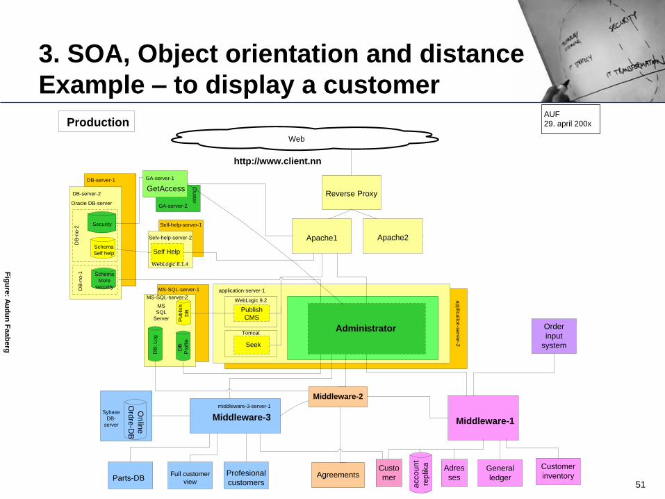
Example – to display a customer
|Administrator
Self Help
Apache1
Reverse Proxy
Apache2
Publish
CMS
Seek
WebLogic 9.2
Tomcat
Pu
blis
h
DB
MS
SQL
Server
WebLogic 8.1.4
Web
Oracle DB-server
application-server-1
MS-SQL-server-2
GA-server-1
DB-server-2
Middleware-3
middleware-3-server-1
Parts-DBFull customer
view
Profesional
customers
General
ledger
ap
plic
atio
n-s
erv
er-2
http://www.client.nn
Utgående
proxy
Switch
/coorp...
DB
: L
og
Custo
mer
Adres
ses
acco
un
t
rep
lika
Middleware-2
Customer
inventoryAgreements
Sybase
DB-
server
GetAccess
GA-server-2
On
line
Ord
re-D
B
Clu
ste
r
Middleware-1
Security
Schema
Self help
DB
:
Pro
file
AUF
29. april 200x
Schema
More
security
Production
Order
input
system
DB-server-1
Selv-help-server-2
Self-help-server-1
DB
-no
-2D
B-n
o-1
MS-SQL-server-1
Fig
ure
: Au
du
n F
aab
erg

52
3. SOA, Object orientation and distance
Challenges
• This distance is correct object orientation. If a developer has an object and
methods that work correctly, he/she shall not worry about the implementation
of these objects.
• Also, in test, on low volumes, this will work perfectly.
• Hibernate – a framework for database access from Java – hides the SQL for
the developer, and present objects. In the background, Hibernates serialises
the object, meaning mapping the object structure to a relational table
structure, and creating the SQL to manipulate this.
• Again, may be challenging in high performance environment.
• In a WAN-environment, be very careful about the network latency, if the
application is “chatty”. Take care to send over chunks of 100 or 1000 rows
from a request, not one by one….
Copyright © 2011 Accenture All Rights Reserved.

3. SOA, Object orientation and distance
Example
DB2
CICS
Batch- process
Large data object is created
High CPU consumption on DB server, Massive impact on other systems
95% is thrown away in the Batch-process
Person register
Person number + status Name Civil status Current adress Current county All previous adresses All previous counties All previous countries Immigration date Citizenship date Bank account
Phone number Mobile number Email adress Foreign stays Person status Description of person status Incapable and date Filial used and 7 more
100% CPU
Person number + status Name Civil status Current adress Current county All previous adresses All previous counties All previous countries Immigration date Citizenship date Bank account
Phone number Mobile number Email adress Foreign stays Person status Description of person status Incapable and date Filial used and 7 more
Copyright © 2011 Accenture All Rights Reserved.

3. SOA, Object orientation and distance
New solution
Small data object created
personnummer + status
Low CPU consumption, short run time
Person nummer + status Run time reduced 90% CPU consumption reduced by 95%. No impact on other systems now.
DB2
CICS
Batch prosess
Person register
Copyright © 2011 Accenture All Rights Reserved.

55
4. Performance engineering
Accenture Offerings
• Accenture Technology Consulting has a performance engineering group.
• Offerings:
– Capacity Modelling: How do I come up with a justifiable, solid capacity plan?
Will this infrastructure support the next go-live‟s volumes? Are these SLAs
acceptable? How do I project load test results to production volumes?
– Performance Testing: To avoid problems after go live, a robust and valid
performance testing effort for new the application and infrastructure is required.
Ensure your application can perform to the SLA objectives.
– Performance Diagnostics: If you skipped the performance test, we may help
you identify and quickly resolve production performance issues. Bottlenecks in
Network, Application, Database, Infrastructure, Architecture are identified and
handled.
Copyright © 2011 Accenture All Rights Reserved.

56
4. Performance engineering
PE through the project phases - challenges
1 . Assumed High Performance .
No EXPLICIT definition of
performance requirements
1 . Design independent of performance requirement
2 . Lack knowledge of Data volumes and scalability
3 . Design reviews
do not focus on performance
1 . Lack of coding guidelines
2 . Code profiling not part of Build
3 . Lack of expertise in profiler tools usage
4 . Code reviews do not focus on Performance
1 . Lack of explicit Performance test plan
2 . Lack of test
environment / test data to simulate production load
3 . Insufficient Load
Stress Stability tests
4 . No Explicit performance sign -
offs due to lack of clear requirements .
1 . Lack of proactive monitoring
2 . Critical problems in production
3 . High time to resolve critical problems
4 . Lack of expertise in monitoring tools
5 . Risk with credibility / possible
penalties
PROBLEMS PROBLEMS PROBLEMS PROBLEMS PROBLEMS
Analysis Design Build Test Run
Copyright © 2011 Accenture All Rights Reserved.

57
1. Introduction
Basic arithmetic
0.000 sec x 6,000,000 = 0 sec
0.012 sec x 6,000,000 = 72000 sec = 20 hours
Many designers think this is the database speed
And this may be the real database
speed
Copyright © 2011 Accenture All Rights Reserved.