languages - easy semestereasysemester.com/sample/solution-manual-for-languages...however, it need...
TRANSCRIPT

download instant at www.easysemester.com
Chapter 2
Languages
3. We prove, by induction on the length of the string, that w = (wR)R for every string w ∈ Σ∗.
Basis: The basis consists of the null string. In this case, (λR)R = (λ)R = λ as desired.
Inductive hypothesis: Assume that (wR)R = w for all strings w ∈ Σ∗ of length n or less.
Inductive step: Let w be a string of length n + 1. Then w = ua and
(wR)R = ((ua)R)R
= (aRuR)R (Theorem 2.1.6)= (auR)R
= (uR)RaR (Theorem 2.1.6)= uaR (inductive hypothesis)= ua= w
8. Let L denote the set of strings over Σ = {a, b} that contain twice as many a’s as b’s. The setL can be defined recursively as follows:
Basis: λ ∈ L
Recursive step: If u ∈ L and u can be written xyzw where x, y, z, w ∈ Σ∗ then
i) xayazbw ∈ L,
ii) xaybzaw ∈ X, and
iii) xbyazaw ∈ X.
Closure: A string u is in L only if it can be obtained from λ using a finite number of appli-cations of the recursive step.
Cleary, every string generated by the preceding definition has twice as many a’s as b’s. A proofby induction on the length of strings demonstrates that every string with twice as many a’sas b’s is generated by the recursive definition. Note that every string in L has length divisibleby three.
Basis: The basis consists of the null string, which satisfies the relation between the numberof a’s and b’s.
Inductive hypothesis: Assume that all strings with twice as many a’s as b’s of length k,0 ≤ k ≤ n, are generated by the recursive definition.
7

download instant at www.easysemester.com
8 CHAPTER 2. LANGUAGES
Inductive step: Let u be a string of length n + 3 with twice as many a’s as b’s. Since ucontains at least three elements, x can be written xayazbw, xaybzaw, or xbyazaw for somex, y, w, z ∈ Σ∗. It follows that xyzw has twice as many a’s as b’s and, by the inductivehypothesis, is generated by the recursive definition. Thus, one additional application of therecursive step produces u from xyzw.
12. Let P denote the set of palindromes defined by the recursive definition and let W = {w ∈ Σ∗ |w = wR}. Establishing that P = W requires demonstrating that each of the sets is a subsetof the other.
We begin by proving that P ⊆ W. The proof is by induction on the number of applications ofthe recursive step in the definition of palindrome required to generate the string.
Basis: The basis consists of strings of P that are generated with no applications of therecursive step. This set consists of λ and a, for every a ∈ Σ. Clearly, w = wR for every suchstring.
Inductive hypothesis: Assume that every string generated by n or fewer applications ofthe recursive step is in W.
Inductive step: Let u be a string generated by n+1 applications of the recursive step. Thenu = awa for some string w and symbol a ∈ Σ, where w is generated by n applications of therecursive step. Thus,
uR = (awa)R
= aRwRaR (Theorem 2.1.6)= awRa= awa (inductive hypothesis)= u
and u ∈ W.
We now show that W ⊆ P. The proof is by induction on the length of the strings in W.
Basis: If length(u) = 0, then w = λ and λ ∈ P by the basis of the recursive definition.Similarly, strings of length one in W are also in P.
Inductive hypothesis: Assume that every string w ∈ W with length n or less is in P.
Inductive step: Let w ∈ W be a string of length n + 1, n ≥ 1. Then w can be written uawhere length(u) = n. Taking the reversal,
w = wR = (ua)R = auR
Since w begins and ends with with same symbol, it may be written w = ava. Again, usingreversals we get
wR = (ava)R
= aRvRaR
= avRa
Since w = wR, we conclude that ava = avRa and v = vR. By the inductive hypothesis, v ∈ P.It follows, from the recursive step in the definition of P, that w = ava is also in P.

download instant at www.easysemester.com
SOLUTIONS TO EXERCISES 9
13. The language L2 consists of all strings over {a, b} of length four. L3, obtained by applying theKleene star operation to L2, contains all strings with length divisible by four. The null string,with length zero, is in L3.
The language L1 ∩ L3 contains all strings that are in both L1 and L3. By being in L1, eachstring must consist solely of a’s and have length divisible by three. Since L3 requires lengthdivisible by four, a string in L1 ∩ L3 must consist only of a’s and have length divisible by 12.That is, L1 ∩ L3 = (a12)∗.
15. Since the null string is not allowed in the language, each string must contain at least one aor one b or one c. However, it need not contain one of every symbol. The +’s in the regularexpression a+b∗c∗ ∪ a∗b+c∗ ∪ a∗b∗c+ ensure the presence of at least one element in eachstring in the language.
21. The set of strings over {a, b} that contain the substrings aa and bb is represented by
(a ∪ b)∗aa(a ∪ b)∗bb(a ∪ b)∗ ∪ (a ∪ b)∗bb(a ∪ b)∗aa(a ∪ b)∗.
The two expressions joined by the ∪ indicate that the aa may precede or follow the bb.
23. The leading a and trailing cc are explicitly placed in the expression
a(a ∪ c)∗b(a ∪ c)∗b(a ∪ c)∗cc.
Any number of a’s and c’s, represented by the expression (a∪ c)∗, may surround the two b’s.
24. At first glance it may seem that the desired language is given by the regular expression
(a ∪ b)∗ab(a ∪ b)∗ba(a ∪ b)∗ ∪ (a ∪ b)∗ab(a ∪ b)∗ba(a ∪ b)∗.
Clearly every string in this language has substrings ab and ba. Every string described by thepreceding expression has length four or more. Have we missed some strings with the desiredproperty? Consider aba, bab, and aaaba. A regular expression for the set of strings containingsubstrings ab and ba can be obtained by adding
(a ∪ b)∗aba(a ∪ b)∗ ∪ (a ∪ b)∗bab(a ∪ b)∗
to the expression above.
26. The language consisting of strings over {a, b} containing exactly three a’s is defined by the reg-ular expression b∗ab∗ab∗ab∗. Applying the Kleene star to the preceding expression producesstrings in which the number of a’s is a multiple of three. However, (b∗ab∗ab∗ab∗)∗ does notcontain strings consisting of b’s alone; the null string is the only string that does have at leastthree a’s. To obtain strings with no a’s, b∗ is concatenated to the end of the preceding expres-sion. Strings consisting solely of b’s are obtained from (b∗ab∗ab∗ab∗)∗b∗ by concatenatingλ from (b∗ab∗ab∗ab∗)∗ with b’s from b∗. The regular expression (b∗ab∗ab∗a)b∗ defines thesame language.
28. In the regular expression(ab ∪ ba ∪ aba ∪ b)∗,
a’s followed by a b are produced by the first component, a’s preceded by a b by the secondcomponent, and two a’s “covered” by a single b by the third component. The inclusion of bwithin the scope of the ∗ operator allows any number additional b’s to occur anywhere in thestring.
Another regular expression for this language is ((a ∪ λ)b(a ∪ λ))∗.

download instant at www.easysemester.com
10 CHAPTER 2. LANGUAGES
31. Every aa in the expression (b ∪ ab ∪ aab)∗ is followed by at least one b, which precludes theoccurrence of aaa. However, every string in this expression ends with b while strings in thelanguage may end in a or aa as well as b. Thus the expression
(b ∪ ab ∪ aab)∗(λ ∪ a ∪ aa)
represents the set of all strings over {a, b} that do not contain the substring aaa.
32. A string can begin with any number of b’s. Once a’s are generated, it is necessary to ensure thatan occurrence of ab is either followed by another b or ends the string. The regular expressionb∗(a ∪ abb+)∗(λ ∪ ab) describes the desired language.
34. To obtain an expression for the strings over {a, b, c} with an odd number of occurrences ofthe substring ab we first construct an expression w defining strings over {a, b, c} that do notcontain the substring ab,
w = b∗(a ∪ cb∗)∗.
Using w, the desired set can be written (wabwab)∗wabw.
37. The regular expression (b∗ab∗a)∗b∗ ∪ (a∗ba∗b)∗a∗ba∗ defines strings over {a, b} with aneven number of a’s or an odd number of b’s. This expression is obtained by combining anexpression for each of the component subsets with the union operation.
38. Exercises 37 and 38 illustrate the significant difference between union and intersection indescribing patterns with regular expressions. There is nothing intuitive about a regular ex-pression for this language. The exercise is given, along with the hint, to indicate the needfor an algorithmic approach for producing regular expressions. A technique accomplish thiswill follow from the ability to reduce finite state machines to regular expressions developed inChapter 6. Just for fun, a solution is
([aa ∪ ab(bb)∗ba] ∪ [(b ∪ a(bb)∗ba)(a(bb)∗a)∗(b ∪ ab(bb)∗a)]
)∗.
39. a) (ba)+(a∗b∗ ∪ a∗)= (ba)+(a∗)(b∗ ∪ λ) (identity 5)= (ba)∗baa∗(b∗ ∪ λ) (identity 4)= (ba)∗ba+(b∗ ∪ λ)
c) Except where noted, each step employs an identity from rule 12 in Table 2.1.
(a ∪ b)∗ = (b ∪ a)∗ (identity 5)= b∗(b ∪ a)∗ (identity 5)= b∗(a∗b∗)∗
= (b∗a∗)∗b∗ (identity 11)= (b ∪ a)∗b∗
= (a ∪ b)∗b∗ (identity 5)
download instant at www.easysemester.com
12 CHAPTER 3. CONTEXT-FREE GRAMMARS
8. The language consisting of the set of strings {anbmc2n+m | m, n > 0} is generated by
S → aScc | aAccA → bAc | bc
For each leading a generated by the S rules, two c’s are produced at the end of the string. Therule A rules generate an equal number of b’s and c’s.
12. A recursive definition of the set of strings over {a, b} that contain the same number of a’s andb’s is given in Example 2.2.3. The recursive definition provides the insight for constructing therules of the context-free grammar
S → λS → SaSbS | SbSaS | SS
that generates the language. The basis of the recursive definition consists of the null string.The first S rule produces this string. The recursive step consists of inserting an a and b ina previously generated string or by concatenating two previously generated strings. Theseoperations are captured by the second set of S rules.
13. An a can be specifically placed in the middle position of a string using the rules
A → aAa | aAb | bAa | bAb | a
The termination of the application of recursive A rules by the rule A → a inserts the symbola into the middle of the string. Using this strategy, the grammar
S → aAa | aAb | bBa | bBb | a | bA → aAa | aAb | bAa | bAb | aB → aBa | aBb | bBa | bBb | b
generates all strings over {a, b} with the same symbol in the beginning and middle positions.If the derivation begins with an S rule that begins with an a, the A rules ensure that an aoccurs in the middle of the string. Similarly, the S and B rules combine to produce stringswith a b in the first and middle positions.
16. The language (a ∪ b)∗aa(a ∪ b)∗bb(a ∪ b)∗ is generated by
G1: S1 → aS1 | bS1 | aAA → aBB → aB | bB | bCC → bDD → aD | bD | λ
G2 generates the strings (a ∪ b)∗bb(a ∪ b)∗aa(a ∪ b)∗
G2: S2 → aS2 | bS2 | bEE → bFF → aF | bF | aGG → aHH → aH | bH | λ

download instant at www.easysemester.com
SOLUTIONS TO EXERCISES 13
A grammar G that generates
(a ∪ b)∗aa(a ∪ b)∗bb(a ∪ b)∗ ∪ (a ∪ b)∗bb(a ∪ b)∗aa(a ∪ b)∗
can be obtained from G1 and G2. The rules of G consist of the rules of G1 and G2 augmentedwith S → S1 | S2 where S is the start symbol of the composite grammar. The alternative inthese productions corresponds to the ∪ in the definition of the language.
While the grammar described above generates the desired language, it is not regular. Therules S → S1 | S2 do not have the form required for rules of a regular grammar. A regulargrammar can be obtained by explicitly replacing S1 and S2 in the S rules with the right-handsides of the S1 and S2 rules. The S rules of the new grammar are
S → aS1 | bS1 | aAS → aS2 | bS2 | bE
The strategy used to modify the rules S → S1 | S2 is an instance of a more general rulemodification technique known as removing chain rules, which will be studied in detail inChapter 4.
20. The language ((a ∪ λ)b(a ∪ λ))∗ is generated by the grammar
S → aA | bB | λA → bBB → aS | bB | λ
This language consists of all strings over {a, b} in which every a is preceded or followed by a b.An a generated by the rule S → aA is followed by a b. An a generated by B → aS is precededby a b.
24. The variables of the grammar indicate whether an even or odd number of ab’s has beengenerated and the progress toward the next ab. The interpretation of the variables is
Variable Parity Progress toward abS even noneA even aB odd noneC odd a
The rules of the grammar are
S → aA | bSA → aA | bBB → aC | bB | λC → aC | bS | λ
A derivation may terminate with a λ-rule when a B or a C is present in the sentential formsince this indicates that an odd number of ab’s have been generated.
25. The objective is to construct a grammar that generates the set of strings over {a, b} containingan even number of a’s or an odd number of b’s. In the grammar,

download instant at www.easysemester.com
14 CHAPTER 3. CONTEXT-FREE GRAMMARS
S → aOa | bEa | bOb | aEb | λEa → aOa | bEa | λOa → aEa | bOa
Ob → aOb | bEb | λEb → aEb | bOb
the Ea and Oa rules generate strings with an even number of a’s. The derivation of a stringwith a positive even number of a’s is initiated by the application of an S rule that generateseither Ea or Oa. The derivation then alternates between occurrences of Ea and Oa until it isterminated with an application of the rule Ea → λ.
In a like manner, the Ob and Eb rules generate strings with an odd number of b’s. Thestring aab can be generated by two derivations; one beginning with the application of the ruleS → aOa and the other beginning with S → aEb.
30. Let G be the grammar S → aSbS | aS | λ. We prove that every prefix of sentential form ofG has at least as many a’s as b’s. We will refer to this condition as the prefix property. Theproof is by induction of the length of derivations of G.
Basis: The strings aSbS, aS and λ are the only sentential forms produced by derivations oflength one. The prefix property is seen to hold for these strings by inspection.
Inductive hypothesis: Assume that every sentential form that can be obtained by a deriva-tion of length n or less satisfies the prefix property.
Inductive step: Let w be a sentential form of G that can be derived using n + 1 ruleapplications. The derivation of w can be written
Sn⇒ uSv ⇒ w
where w is obtained by applying an S rule to uSv. By the inductive hypothesis uSv satisfiesthe prefix property. A prefix of w consists of a prefix of uSv with the S replaced by λ, aS oraSbS. Thus w also satisfies the prefix property.
32. a) The language of G is (a+b+)+.
b) The rules S → aS and S → Sb allow the generation of leading a’s or trailing b’s in anyorder. Two leftmost derivations for the string aabb are
S ⇒ aS S ⇒ Sb⇒ aSb ⇒ aSb⇒ aabb ⇒ aabb
c) The derivation trees corresponding to the derivations of (b) are
INSERT FIGURE Chapter 3: Exercise 32 c) HERE
d) The unambiguous regular grammar
S → aS | aAA → bA | bS | b
is equivalent to G and generates strings unambiguously producing the terminals in a left-to-right manner. The S rules generate the a’s and the A rules generate the b’s. Theprocess is repeated by the application of the rule A → bS or terminated by an applicationof A → b.

download instant at www.easysemester.com
SOLUTIONS TO EXERCISES 15
33. a) The string consisting of ten a’s can be produced by two distinct derivations; one consistingof five applications of the rule S → aaS followed by the λ-rule and the other consistingof two applications of S → aaaaaS and the λ-rule.To construct an unambiguous grammar that generates L(G), it is necessary to determineprecisely which strings are in L(G). The rules S → λ and S → aaS generate all stringswith an even number of a’s. Starting a derivation with a single application of S → aaaaaSand completing it with applications of S → aaS and S → λ produces strings of length5, 7, 9, . . . . The language of G consists of all strings of a’s except for a and aaa. Thislanguage is generated by the unambiguous grammar
S → λ | aa | aaaAA → aA | a
d) L(G) is the set {λ}∪{aibj | i > 1, j > 0}. The null string is generated directly by the ruleS → λ. The rule S → AaSbB generates one a and one b. Applications of S → AaSbB,A → a, A → aA, and B → bB generate additional a’s and b’s. The rule A → a guaranteesthat there are two or more a’s in every string nonnull in L(G).To show that G is ambiguous we must find a string w ∈ L(G) that can be generated bytwo distinct leftmost derivations. The prefix of a’s can be generated either by applicationsof the rule S → AaSbB or by the A rules. Consider the derivation of the string aaaabbin which two a’s are generated by applications of the S rule.
Derivation Rule
S ⇒ AaSbB S → AaSbB⇒ aaSbB A → a⇒ aaAaSbBbB S → AaSbB⇒ aaaaSbBbB A → a⇒ aaaabBbB S → λ⇒ aaaabbB B → λ⇒ aaaabb B → λ
The string can also be derived using the rules A → aA and A → a to generate the a’s.
Derivation Rule
S ⇒ AaSbB S → AaSbB⇒ aAaSbB A → aA⇒ aaAaSbB A → aA⇒ aaaaSbB A → a⇒ aaaabB S → λ⇒ aaaabbB B → bB⇒ aaaabb B → λ
The two distinct leftmost derivations of aaaabb demonstrate the ambiguity of G.The regular grammar
S → aA | λA → aA | aBB → bB | b
generates strings in L(G) in a left-to-right manner. The rules S → aA and A → aBguarantee the generation of at least two a’s in every nonnull string. The rule B → b,whose application completes a derivation, ensures the presence of at least one b.

download instant at www.easysemester.com
16 CHAPTER 3. CONTEXT-FREE GRAMMARS
e) The variable A generates strings of the form (ab)i and B generates aibi for all i ≥ 0.The only strings in common are λ and ab. Each of these strings can be generated by twodistinct leftmost derivations.To produce an unambiguous grammar, it is necessary to ensure that these strings aregenerated by only one of A and B. Using the rules
S → A | BA → abA | ababB → aBb | λ,
λ and ab are derivable only from the variable B.
34. a) The grammar G was produced in Exercise 33 d) to generate the language {λ} ∪ {aibj |i > 0, j > 1} unambiguously. A regular expression for this language is a+b+b ∪ λ.
b) To show that G is unambiguous it is necessary to show that there is a unique leftmostderivation of every string in L(G). The sole derivation of λ is S ⇒ λ. Every other stringin L(G) has the form aibj where i > 0 and j > 1. The derivation of such a string has theform
Derivation Rule
S =⇒ aA S → aAi−1=⇒ aiA A → aA=⇒ aibB A → bBj−2=⇒ aibbj−2B B → bB=⇒ aibbj−2b B → b= aibj
At each step there is only one rule that can be applied to successfully derive aibj . Initiallythe S rule that produces an a must be employed, followed by exactly i − 1 applicationsof the rule A → aA. Selecting the other A rule prior to this point would produce a stringwith to few a’s. Using more than i− 1 applications would produce too many a’s.After the generation of ai, the rule A → bB begins the generation of the b’s. Anydeviation from the pattern in the derivation above would produce the wrong numberof b’s. Consequently, there is only one leftmost derivation of aibj and the grammar isunambiguous.
39. a) The rules S → aABb, A → aA, and B → bB of G1 are produced by the derivationsS ⇒ AABB ⇒ aABB ⇒ aABb, A ⇒ AA ⇒ aA, and B ⇒ BB ⇒ bB using the rules ofG2. Thus every rule of G1 is either in G2 or derivable in G2.Now if w is derivable in G1, it is also derivable in G2 by replacing the application of a ruleof G1 by the sequence of rules of G2 that produce the same transformation. If follows theL(G1) ⊆ L(G2.
b) The language of G1 is aa+b+b. Since the rules
A → AA | a
generate a+ andB → BB | b
generate b+, the language of G2 is a+a+b+b+ = aa+b+b.

download instant at www.easysemester.com
SOLUTIONS TO EXERCISES 17
40. A regular grammar is one with rules of the form A → aB, A → a, and A → λ, where A,B ∈ Vand a ∈ Σ. The rules of a right-linear grammar have the form A → λ, A → u, and A → uB,where A,B ∈ V and u ∈ Σ+. Since every regular grammar is also right-linear, all regularlanguages are generated by right-linear grammars.
We now must show that every language generated by a right-linear grammar is regular. Let Gbe a right-linear grammar. A regular grammar G′ that generates L(G) is constructed from therules of G. Rules of the form A → aB, A → a and A → λ in G are also in G′. A right-linearrule A → a1 . . . an with n > 1 is transformed into a sequence of rules
A → a1T1
T1 → a2T2
...Tn−1 → an
where Ti are variables not occurring in G. The result of the application of the A → u of G isobtained by the derivation
A ⇒ a1T1 ⇒ · · · ⇒ a1 . . . an−1Tn−1 ⇒ a1 . . . an
in G′.
Similarly, rules of the form A → a1 . . . anB, with n > 1, can be transformed into a sequenceof rules as above with the final rule having the form Tn−1 → anB. Clearly, the grammar G′
constructed in this manner generates L(G).

download instant at www.easysemester.com
18 CHAPTER 3. CONTEXT-FREE GRAMMARS

download instant at www.easysemester.com
Chapter 4
Normal Forms for Context-FreeGrammars
3. An equivalent essentially noncontracting grammar GL with a nonrecursive start symbol isconstructed following the steps given in the proof of Theorem 4.2.3. Because S is recursive, anew start symbol S′ and the rule S′ → S is added to GL are added to GL.
The set of nullable variables is {S′, S, A,B}. All possible derivations of λ from the nullablevariables are eliminated by the addition of five S rules, one A rule, and one B rule. Theresulting grammar is
S′ → S | λS → BSA | BS | SA | BA | B | S | AB → Bba | baA → aA | a
8. Following the technique of Example 4.3.1, an equivalent grammar GC that does not containchain rules is constructed. For each variable, Algorithm 4.3.1 is used to obtain the set ofvariables derivable using chain rules.
CHAIN(S) = {S, A, B, C}CHAIN(A) = {A,B, C}CHAIN(B) = {B,C, A}CHAIN(C) = {C, A, B}
These sets are used to generate the rules of GC according to the technique of Theorem 4.3.3,producing the grammar
S → aa | bb | ccA → aa | bb | ccB → aa | bb | ccC → aa | bb | cc
In the grammar obtained by this transformation, it is clear that the A, B, and C rules do notcontribute to derivations of terminal strings.
19

download instant at www.easysemester.com
20 CHAPTER 4. NORMAL FORMS
15. An equivalent grammar GU without useless symbols is constructed in two steps. The first stepinvolves the construction of a grammar GT that contains only variables that derive terminalstrings. Algorithm 4.4.2 is used to construct the set TERM of variables which derive terminalstrings.
Iteration TERM PREV
0 {D,F, G} -1 {D,F, G,A} {D,F, G}2 {D,F, G,A, S} {D,F, G,A}3 {D,F, G,A, S} {D,F, G,A, S}
Using this set, GT is constructed.
VT = {S, A,D, F, G}ΣT = {a, b}PT : S → aA
A → aA | aDD → bD | bF → aF | aG | aG → a | b
The second step in the construction of GU involves the removal of all variables from GT thatare not reachable from S. Algorithm 4.4.4 is used to construct the set REACH of variablesreachable from S.
Iteration REACH PREV NEW
0 {S} ∅ -1 {S, A} {S} {S}2 {S, A,D} {S, A} {A}3 {S, A,D} {S, A,D} {D}
Removing all references to variables in the set VT − REACH produces the grammar
VU = {S, A,D}ΣU = {a, b}PU : S → aA
A → aA | aDD → bD | b
19. To convert G to Chomsky normal form, we begin by transforming the rules of G to the formS → λ, A → a, or A → w where w is a string consisting solely of variables.
S → XAY B | ABC | aA → XA | aB → Y BZC | bC → XY ZX → aY → bZ → c

download instant at www.easysemester.com
SOLUTIONS TO EXERCISES 21
The transformation is completed by breaking each rule whose right-hand side has length greaterthan 2 into a sequence of rules of the form A → BC.
S → XT1 | AT3 | aT1 → AT2
T2 → Y BT3 → BCA → XA | aB → Y T4 | bT4 → BT5
T5 → ZCC → XT6
T6 → Y ZX → aY → bZ → c
24. a) The derivation of a string of length 0, S ⇒ λ, requires one rule application.A string of length n > 0 requires 2n− 1; n− 1 rules of the form A → BC and n rules ofthe form A → a.
b) The maximum depth derivation tree for a string of length 4 has the form
INSERT FIGURE Chapter 4: Exercise 24 b) HERE
Generalizing this pattern we see that the maximum depth of the derivation tree of a stringof length n > 0 is n. The depth of the derivation tree for the derivation of λ is 1.
c) The minimum depth derivation tree of a string of length 4 has the form
INSERT FIGURE Chapter 4: Exercise 24 c) HERE
Intuitively, the minimum depth is obtained when the tree is the “bushiest” possible. Theminimum depth of a derivation tree for a string of length n > 0 is dlg(n) + 1e.
28. To obtain an equivalent grammar with no direct left recursion, the rule modification thatremoves direct left recursion is applied to the A and B rules producing
S → A | CA → BX | aX | B | aX → aBX | aCX | aB | aCB → CbY | CbY → bY | bC → cC | c
The application of an A rule generates B or a and the X rule produces elements of the formdescribed by (aB ∪ aC)+ using right recursion.
Similarly, the B and Y rules produce Cbb∗ using the right recursive Y rule to generate b+.

download instant at www.easysemester.com
22 CHAPTER 4. NORMAL FORMS
32. The transformation of a grammar G from Chomsky normal form to Greibach normal form isaccomplished in two phases. In the first phase, the variables of the grammar are numberedand an intermediate grammar is constructed in which the first symbol of the right-hand sideof every rule is either a terminal or a variable with a higher number than the number of thevariable on the left-hand side of the rule. This is done by removing direct left recursion andby applying the rule replacement schema of Lemma 4.1.3. The variables S, A, B, and C arenumbered 1, 2, 3, and 4 respectively. The S rules are already in the proper form. Removingdirect left recursion from the A rules produces the grammar
S → AB | BCA → aR1 | aB → AA | CB | bC → a | bR1 → BR1 | B
Applying the rule transformation schema of Lemma 4.1.3, the ruleB → AA can be converted into the desired form by substituting for the first A, resultingin the grammar
S → AB | BCA → aR1 | aB → aR1A | aA | CB | bC → a | bR1 → BR1 | B
The second phase involves transformation of the rules of the intermediate grammar to en-sure that the first symbol of the right-hand side of each rule is a terminal symbol. Workingbackwards from the C rules and applying Lemma 4.1.3, we obtain
S → aR1B | aB | aR1AC | aAC | aBC | bBC | bCA → aR1 | aB → aR1A | aA | aB | bB | bC → a | bR1 → BR1 | B
Finally, Lemma 4.1.3 is used to transform the R1 rules created in the first phase into theproper form, producing the Greibach normal form grammar
S → aR1B | aB | aR1AC | aAC | aBC | bBC | bCA → aR1 | aB → aR1A | aA | aB | bB | bC → a | bR1 → aR1AR1 | aAR1 | aBR1 | bBR1 | bR1
→ aR1A | aA | aB | bB | b
35. We begin by showing how to reduce the length of strings on the right-hand side of the rulesof a grammar in Greibach normal form. Let G = (V, Σ, S, P) be a grammar in Greibachnormal form in which the maximum length of the right-hand side of a rule is n, where n is anynatural number greater than 3. We will show how to transform G to a Greibach normal formgrammar G′ in which the right-hand side of each rule has length at most n− 1.

download instant at www.easysemester.com
SOLUTIONS TO EXERCISES 23
If a rule already has the desired form, no change is necessary. We will outline the approachto transform a rule of the form A → aB2 · · ·Bn−1Bn into a set of rules of the desired form.The procedure can be performed on each rule with right-hand side of length n to produce agrammar in which the right-hand side of each rule has length at most n− 1.
A new variable [Bn−1Bn] is added to grammar and the rule
A → aB2 · · ·Bn−1Bn
is replaced with the ruleA → aB2 · · ·Bn−2[Bn−1Bn]
whose right-hand side has length n − 1. It is now necessary to define the rules for the newvariable [Bn−1Bn]. Let the Bn−1 rules of G be
Bn−1 → β1u1 | β1u2 | · · · | βmum,
where βi ∈ Σ, ui ∈ V∗, and length(βiui) ≤ n. There are three cases to consider in creatingthe new rules.
Case 1: length(βiui) ≤ n− 2. Add the rule
[Bn−1Bn] → βiuiBn
to G′.
Case 2: length(βiui) = n−1. In this case, the Bn−1 rule can be written Bn−1 → βiC2 · · ·Cn−1.Create a new variable [Cn−1Bn] and add the rule
Bn−1 → βiC2 · · ·Cn−2[Cn−1Bn]
to G′.
Case 3: length(βiui) = n. In this case, the Bn−1 rule can be written Bn−1 → βiC2 · · ·Cn−1Cn.Create two new variables [Cn−2Cn−1] and [CnBn] and add the rule
Bn−1 → βiC2 · · ·Cn−3[Cn−2Cn−1][CnBn]
to G′.
Each of the rules generated in cases 1, 2, and 3 have right-hand sides of length n − 1. Theprocess must be repeated until rules have been created for each variable created by the ruletransformations.
The construction in case 3 requires the original rule to have at least three variables. Thislength reduction process can be repeated until each rule has a right-hand side of length atmost 3. A detailed proof that this construction produces an equivalent grammar can be foundin Harrison1.
1M. A. Harrison, Introduction to Formal Languages, Addison-Wesley, 1978

download instant at www.easysemester.com
24 CHAPTER 4. NORMAL FORMS

download instant at www.easysemester.com
Chapter 5
Finite Automata
1. a) The state diagram of M is
INSERT FIGURE Chapter 5: Exercise 1 a) HERE
b) i) [q0, abaa] ii) [q0, bbbabb]` [q0, baa] ` [q1, bbabb]` [q1, aa] ` [q1, babb]` [q2, a] ` [q1, abb]` [q2, λ] ` [q2, bb]
` [q0, b]` [q1, λ]
iii) [q0, bababa] iv) [q0, bbbaa]` [q1, ababa] ` [q1, bbaa]` [q2, baba] ` [q1, baa]` [q0, aba] ` [q1, aa]` [q0, ba] ` [q2, a]` [q1, a] ` [q2, λ]` [q2, λ]
c) The computations in (i), (iii), and (iv) terminate in the accepting state q2. Therefore,the strings abaa, bababa, and bbbaa are in L(M).
d) Two regular expressions describing L(M) are a∗b+a+(ba∗b+a+)∗ and (a∗b+a+b)∗a∗b+a+.
4. The proof is by induction on length of the input string. The definitions of δ and δ′ are thesame for strings of length 0 and 1.
Assume that δ(qi, u) = δ′(qi, u) for all strings u of length n or less. Let w = bva be a string oflength of n + 1, with a, b ∈ Σ and length(v) = n− 1.
δ(qi, w) = δ(qi, bva)
= δ(δ(qi, bv), a) (definition of δ)
= δ(δ′(qi, bv), a) (inductive hypothesis)
= δ(δ′(δ(qi, b), v), a) (definition of δ′)
25

download instant at www.easysemester.com
26 CHAPTER 5. FINITE AUTOMATA
Similarly,
δ′(qi, w) = δ′(qi, bva)
= δ′(δ(qi, b), va) (definition of δ′)
= δ(δ(qi, b), va) (inductive hypothesis)
= δ(δ(δ(qi, b), v), a) (definition of δ)
= δ(δ′(δ(qi, b), v), a) (inductive hypothesis)
Thus δ(qi, w) = δ′(qi, w) for all strings w ∈ Σ∗ as desired.
5. The DFA
INSERT FIGURE Chapter 5: Exercise 5 HERE
that accepts a∗b∗c∗ uses the loops in states q0, q1, and q2 to read a’s, b’s, and c’s. Anydeviation from the prescribed order causes the computation to enter q3 and reject the string.
8. A DFA that accepts the strings over {a, b} that do not contain the substring aaa is given bythe state diagram
INSERT FIGURE Chapter 5: Exercise 8 HERE
The states are used to count the number of consecutive a’s that have been processed. Whenthree consecutive a’s are encountered, the DFA enters state q3, processes the remainder of theinput, and rejects the string.
15. The DFA
INSERT FIGURE Chapter 5: Exercise 15 HERE
accepts strings of even length over {a, b, c} that contain exactly one a. A string accepted bythis machine must have exactly one a and the total number of b’s and c’s must be even. Acomputation that processes an even number of b’s and c’s terminates in state q0 or q1. Statesq1 or q3 are entered upon processing a single a. The state q1 represents the combination of thetwo conditions required for acceptance. Upon reading a second a, the computation enters thenonaccepting state q4 and rejects the string.
20. The states of the machine are used to count the number of symbols processed since an a hasbeen read or since the beginning of the string, whichever is smaller.
INSERT FIGURE Chapter 5: Exercise 20 HERE

download instant at www.easysemester.com
SOLUTIONS TO EXERCISES 27
A computation is in state qi if the previous i elements are not a’s. The computation with aninput string that contains a substring of length four without an a halts in state q3 withoutprocessing the complete string. Consequently, any such string is rejected; all other stringsaccepted.
21. The DFA to accept this language differs from the machine in Exercise 20 by requiring everyfourth symbol to be an a. The first a may occur at position 1, 2, 3, or 4. After reading thefirst a, the computation enters a cycle checking for the pattern bbba.
INSERT FIGURE Chapter 5: Exercise 21 HERE
Strings of length 3 or less are accepted, since the condition is vacuously satisfied.
23. a) The transition table for the machine M is
δ a bq0 {q0, q1} ∅q1 ∅ {q1, q2}q2 {q0, q1} ∅
b) [q0, aaabb] [q0, aaabb]` [q1, aabb] ` [q0, aabb]
` [q1, abb]
[q0, aaabb] [q0, aaabb]` [q0, aabb] ` [q0, aabb]` [q0, abb] ` [q0, abb]` [q1, bb] ` [q0, bb]` [q1, b]` [q1, λ]
[q0, aaabb]` [q0, aabb]` [q0, abb]` [q1, bb]` [q1, b]` [q2, λ]
c) Yes, the final computation above reads the entire string and halts in the accepting stateq2.
d) A regular expressions for L(M) is a+b+(ab+ ∪ a+ab+)∗. Processing a+b+ leaves thecomputation in state q2. After arriving at q2 there are two ways to leave and return,taking the cycle q0, q1, q2 or the cycle q1, q2. The first path processes a string froma+ab+ and the second ab+. This expression can be reduced to (a+b+)+.
25. c) The NFA
INSERT FIGURE Chapter 5: Exercise 25 c) HERE

download instant at www.easysemester.com
28 CHAPTER 5. FINITE AUTOMATA
accepts the language (abc)∗a∗. Strings of the form (abc)∗ are accepted in q0. State q3
accepts (abc)∗a+.
29. The set of strings over {a, b} whose third to the last symbol is b is accepted by the NFA
INSERT FIGURE Chapter 5: Exercise 29 HERE
When a b is read in state q1, nondeterminism is used to choose whether to enter state q1
or remain in state q0. If q1 is entered upon processing the third to the last symbol, thecomputation accepts the input. A computation that enters q1 in any other manner terminatesunsuccessfully.
39. Algorithm 5.6.3 is used to construct a DFA that is equivalent to the NFA M in Exercise 17.Since M does not contain λ-transitions, the input transition function used by the algorithm isthe transition function of M. The transition table of M is given in the solution to Exercise 17.
The nodes of the equivalent NFA are constructed in step 2 of Algorithm 5.6.3. The generationof Q′ is traced in the table below. The start state of the determininstic machine is {q0}, whichis the λ-closure of q0. The algorithm proceeds by choosing a state X ∈ Q′ and symbol a ∈ Σfor which there is no arc leaving X labeled a. The set Y consists of the states that may beentered upon processing an a from a state in X.
X input Y Q′
Q′ := {{q0}}{q0} a {q0, q1} Q′ := Q′ ∪ {{q0, q1}}{q0} b ∅ Q′ := Q′ ∪ {∅}
{q0, q1} a {q0, q1}{q0, q1} b {q1, q2} Q′ := Q′ ∪ {{q1, q2}}
∅ a ∅∅ b ∅
{q1, q2} a {q0, q1}{q1, q2} b {q1, q2}
The accepting state is {q1, q2}. The state diagram of the deterministic machine is
INSERT FIGURE Chapter 5: Exercise 39 HERE
43. To prove that qm is equivalent to qn we must show that δ(qm, w) ∈ F if, and only if, δ(qn, w) ∈F for every string w ∈ Σ∗.
Let w be any string over Σ. Since qi and qj are equivalent, δ(qi, uw) ∈ F if, and only if,δ(qj , uw) ∈ F. The equivalence of qm and qn follows since δ(qi, uw) = δ(qm, w) and δ(qn, uw) =δ(qn, w).
44. Let δ′([qi], a) = [δ(qi, a)] be the transition function defined on classes of equivalent states of aDFA and let qi and qj be two equivalent states. To show that δ′ is well defined, we must showthat δ′([qi], a) = δ′([qj ], a).
If δ′([qi], a)qm and δ′([qj ], a) = qn, this reduces to showing that [qm] = [qn]. However, thisequality follows from the result in Exercise 43.

download instant at www.easysemester.com
Chapter 6
Properties of Regular Languages
2. a) This problem illustrates one technique for determining the language of a finite automatonwith more than one accepting. The node deletion algorithm must be employed individu-ally for each accepting state. Following this strategy, a regular expression is obtained bydeleting nodes from the graphs
INSERT FIGURE Chapter 6: Exercise 2 a) I HERE
Deleting q1 and q2 from G1 produces
INSERT FIGURE Chapter 6: Exercise 2 a) II HERE
with the corresponding regular expression b∗. Removing q2 from G2 we obtain
INSERT FIGURE Chapter 6: Exercise 2 a) III HERE
accepting b∗a(ab+)∗. Consequently, the original NFA accepts strings of the form b∗ ∪b∗a(ab+)∗.
5. a) Associating the variables S, A, and B with states q0, q1, and q2 respectively, the regulargrammar
S → aA | λA → aA | aB | bSB → bA | λ
is obtained from the arcs and the accepting states of M.
b) A regular expression for L(M) can be obtained using the node deletion process. Deletingthe state q1 produces the graph
INSERT FIGURE Chapter 6: Exercise 5 b) HERE
29

download instant at www.easysemester.com
30 CHAPTER 6. PROPERTIES OF REGULAR LANGUAGES
The set of strings accepted by q2 is described by the regular expression (a+b)∗aa∗a(ba+∪ba∗b(a+b)∗aa∗a)∗.By deleting states q2 then q1, we see that q0 accepts (a(a ∪ ab)∗b)∗. The language ofM is the union of the strings accepted by q0 and q2.
6. Let G be a regular grammar and M the NFA that accepts L(G) obtained by the constructionin Theorem 6.3.1. We will use induction on the length of the derivations of G to show thatthere is a computation [q0, w] ∗ [C, λ] in M whenever there is a derivation S
∗⇒ wC in G.
The basis consists of derivations of the form S ⇒ aC using a rule S → aC. The rule producesthe transition δ(q0, a) = C in M and the corresponding derivation is [q0, a] ` [C, λ] as desired.
Now assume that [q0, w] ∗ [C, λ] whenever there is a derivation Sn⇒ wC.
Let S∗⇒ wC be a computation of length n + 1. Such a derivation can be written
Sn⇒ uB
uaC,
where B → aC is a rule of G. By the inductive hypothesis, there is a computation [q0, u] `∗ [B, λ]. Combining the transition δ(a,B) = C obtained from the rule B → aC with thepreceding computation produces
[q0, w] = [q0, ua]∗ [B, a]` [C, λ]
as desired.
7. a) Let L be any regular language over {a, b, c} and let L′ be the language consisting ofall strings over {a, b, c} that end in aa. L′ is regular since it is defined by the regularexpression (a ∪ b ∪ c)∗aa. The set
L ∩ L′ = {w | w ∈ L and w contains an a},which consists of all strings in L that end with aa, is regular by Theorem 6.4.3.
11. a) Let G = (V, Σ, S, P) be a regular grammar that generates L. Without loss of generality,we may assume that G does not contain useless symbols. The algorithm to remove uselesssymbols, presented in Section 4.4, does not alter the form of rules of the grammar. Thusthe equivalent grammar obtained by this transformation is also regular.Derivations in G have the form S
∗⇒ uA∗⇒ uv where u, v ∈ Σ∗. A grammar G′ that
generates P = {u | uv ∈ L}, the set of prefixes of L, can be constructed by augmentingthe rules of G with rules A → λ for every variable A ∈ V. The prefix u is produced bythe derivation S
∗⇒ uA ⇒ u in G′.
12. A DFA M′ that accepts the language L′ can be constructed from a DFA M = (Q, Σ, δ, q0, F)that accepts L. The states of M′ are ordered pairs of the form [qi, X], where qi ∈ Q and X is asubset of Q. Intuitively (but not precisely), the state qi represents the number of transitionsfrom the start state when processing a string and the set X consists of states that require thesame number of transitions to reach an accepting state.
The construction of the states Q′ and the transition function δ′ of M′ is iterative. The startstate of the machine is the ordered pair [q0,F]. For each state [qi, X] and symbol a such thatδ([qi, X], a) is undefined, the transition is created by the rule
δ([qi, X], a) = [qi(a),Y],

download instant at www.easysemester.com
SOLUTIONS TO EXERCISES 31
where Y = {qj | δ(qj , a) ∈ X}. If it is not already in Q′, the ordered pair [qi(a), Y] is addedto the states of M′. The process is repeated until a transition is defined for each state-symbolpair.
A state [qi,X] is accepting if qi ∈ X. Back to the intuition, this occurs when the number oftransitions from the start state is the same as the number of transitions needed to reach anaccepting state. That is, when half of a string in L has been processed.
13. b) To show that the set P of even length palindromes is not regular, it suffices to findsequences of strings ui and vi, i = 0, 1, 2, . . . , from {a, b}∗ that satisfy
i) uivi ∈ P, for i ≥ 0ii) uivj 6∈ P whenever i 6= j.
Let ui = aib and vi = bai. Then uivi is the palindrome aibbai. For i 6= j, the stringuivj = aibbaj is not in P. We conclude, by Corollary 6.5.2, that P is not regular.
14. b) Assume that L = {anbm | n < m} is regular. Let k be the number specified by thepumping lemma and z be the string akbk+1. By the pumping lemma, z can be writtenuvw where
i) v 6= λ
ii) length(uv) ≤ k
iii) uviw ∈ L for all i ≥ 0.
By condition (ii), v consists solely of a’s. Pumping v produces the string uv2w thatcontains at least as many a’s as b’s. Thus uv2w 6∈ L and L is not regular.
e) The language L consists of strings of the form λ, a, ab, aba, abaa, abaab, and so forth.Assume that L is regular and let z = abaab · · · bak−1bakb, where k is the number specifiedby the pumping lemma. We will show that there is no decomposition z = uvw in whichv satisfies the conditions of the pumping lemma.The argument utilizes the number of b’s in the substring v. There are three cases toconsider.Case 1: v has no b’s. In this case, the string uv0w has consecutive sequences of a’s inwhich the second sequence has at most the same number of a’s as its predecessor. Thusuv0w 6∈ L.Case 2: v has one b. In this case, v has the form asbat and is obtained from a substringbajbaj+1b in z. The string uv2w obtained by pumping v has a substring bajbas+tbaj+1b,which does not follow pattern of increasing the number of a’s by one in each subsequentsubstring of a’s. Thus uv2w 6∈ L.Case 3: v has two or more b’s. In this case, v contains a substring batb. Pumping vproduces two substrings of the form batb in uv2w. Since no string in L can have twodistinct substrings of this form, uv2w 6∈ L.Thus there is no substring of z that satisfies the conditions of the pumping lemma andwe conclude the L is not regular.
17. b) Let L1 be a nonregular language and L2 be a finite language. Since every finite languageis regular, L1 ∩ L2 is regular. Now assume that L1 − L2 is regular. By Theorem 6.4.1,
L1 = (L1 − L2) ∪ (L1 ∩ L2)
is regular. But this is a contradiction, and we conclude that L1 − L2 is not regular. Thisresult shows that a language cannot be “a little nonreguar”; removing any finite numberof elements from a nonregular set cannot make it regular.

download instant at www.easysemester.com
32 CHAPTER 6. PROPERTIES OF REGULAR LANGUAGES
18. a) Let L1 =a∗b∗ and L2 = {aibi | i ≥ 0}. Then L1 ∪ L2 = L1, which is regular.b) In a similar manner, let L1 = ∅ and L2 = {aibi | i ≥ 0}. Then L1 ∪ L2 = L2, which is
nonregular.
19. a) The regular languages over a set Σ are constructed using the operations union, concate-nation, and Kleene star. We begin by showing that these set operations are preserved byhomomorphisms. That is, for sets X and Y and homomorphism h
i) h(XY) = h(X)h(Y)ii) h(X ∪ Y) = h(X) ∪ h(Y)iii) h(X∗) = h(X)∗.The set equality h(XY) = h(X)h(Y) can be obtained by establishing the inclusions h(XY)⊆ h(X)h(Y) and h(X)h(Y) ⊆ h(XY).Let x be an element of h(XY). Then x = h(uv) for some u ∈ X and v ∈ Y. Since h is ahomomorphism, x = h(u)h(v) and x ∈ h(X)h(Y). Thus h(XY) ⊆ h(X)h(Y). To establishthe opposite inclusion, let x be an element in h(X)h(Y). Then x = h(u)h(v) for some u ∈X and v ∈ Y. As before, x = h(uv) and h(X)h(Y) ⊆ h(XY). The other two set equalitiescan be established by similar arguments.Now let Σ1 and Σ2 be alphabets, X a language over Σ1, and h a homomorphism from Σ∗1to Σ∗2. We will use the recursive definition of regular sets to show that h(X) is regularwhenever X is. The proof is by induction on the number of applications of the recursivestep in Definition 2.3.1 needed to generate X.
Basis: The basis consists of regular sets ∅, {λ}, and {a} for every a ∈ Σ1. The ho-momorphic images of these sets are the sets ∅, {λ}, and {h(a)}, which are regular overΣ2.
Inductive hypothesis: Now assume that the homomorphic image of every regular setdefinable using n or fewer applications of the recursive step is regular.
Inductive step: Let X be a regular set over Σ1 definable by n + 1 applications of therecursive step in Definition 2.3.1. Then X can be written Y ∪ Z, YZ, or Y∗ where Y andZ are definable by n or fewer applications. By the inductive hypothesis, h(Y) and h(Z)are regular. It follows that h(X), which is either h(Y)∪ h(Z), h(Y)h(Z), or h(Y)∗, is alsoregular.
21. For every regular grammar G = (V, Σ, S, P) there is a corresponding a left-regular grammarG′ = (V, Σ, S, P′), defined by
i) A → Ba ∈ P′ if, and only if, A → aB ∈ Pii) A → a ∈ P′ if, and only if, A → a ∈ Piii) A → λ ∈ P′ if, and only if, A → λ ∈ P.
The following Lemma establishes a relationship between regular and left-regular grammars.
Lemma. Let G and G′ be corresponding regular and left-regular grammars. Then L(G′) =L(G)R.
The lemma can be proven by showing that S∗⇒ u in G if, and only if, S
∗⇒ uR in G′. Theproof is by induction on the length of the derivations.
a) Let L be a language generated by a left-regular grammar G′. By the preceding lemma,the corresponding regular grammar G generates LR. Since regularity is preserved bythe operation of reversal, (LR)R = L is regular. Thus every language generated by aleft-regular grammar is regular.

download instant at www.easysemester.com
SOLUTIONS TO EXERCISES 33
b) Now we must show that every regular language is generated by a left-regular grammar.If L is a regular language, then so is LR. This implies that there is a regular grammar Gthat generates LR. The corresponding left-regular grammar G′ generates (LR)R = L.
29. The ≡M equivalence class of a state qi consists of all strings for which the computation of Mhalts in qi. The equivalence classes of the DFA in Example 5.3.1 are
state equivalence classq0 (a ∪ ba)∗
q1 a∗b(a+b)∗
q2 a∗b(a+b)∗b(a ∪ b)∗
31. Let M = (Q, Σ, δ, q0, F) be the minimal state DFA that accepts a language L as constructedby Theorem 6.7.4 and let n be the number of states of M. We must show that any other DFAM′ with n states that accepts L is isomorphic to M.
By Theorem 6.7.5, the ≡M equivalence classes of the states M are identical to the ≡L equiv-alence classes of the language L.
By the argument in Theorem 6.7.5, each ≡M′ equivalence class is a subset of a ≡L equivalenceclass. Since there are same number of ≡M′ and ≡L equivalence classes, the equivalence classesdefined by L and M′ must be identical.
The start state in each machine is the state associated with [λ]≡L. Since the transition functioncan be obtained from the ≡L equivalence classes as outlined in Theorem 6.7.4, the transitionfunctions of M and M′ are identical up to the names given to the states.

download instant at www.easysemester.com
34 CHAPTER 6. PROPERTIES OF REGULAR LANGUAGES

download instant at www.easysemester.com
Chapter 7
Pushdown Automata andContext-Free Languages
1. a) The PDA M accepts the language {aibj | 0 ≤ j ≤ i}. Processing an a pushes A onto thestack. Strings of the form ai are accepted in state q1. The transitions in q1 empty thestack after the input has been read. A computation with input aibj enters state q2 uponprocessing the first b. To read the entire input string, the stack must contain at least jA’s. The transition δ(q2, λ, A) = [q2, λ] will pop any A’s remaining on the stack.
b) The state diagram of M is
INSERT FIGURE chapter 7: exercise 1 b) HERE
d) To show that the strings aabb and aaab are in L(M), we trace a computation of M thataccepts these strings.
State String Stackq0 aabb λq0 abb Aq0 bb AAq2 b Aq2 λ λ
State String Stackq0 aaab λq0 aab Aq0 ab AAq0 b AAAq2 λ AAq2 λ Aq2 λ λ
Both of these computations terminate in the accepting state q2 with an empty stack.
3. d) The pushdown automaton defined by the transitions
δ(q0, λ, λ) = {[q1, C]}δ(q1, a, A) = {[q2, A]}
35

download instant at www.easysemester.com
36 CHAPTER 7. PUSHDOWN AUTOMATA
δ(q1, a, C) = {[q2, C]}δ(q1, b, B) = {[q3, B]}δ(q1, b, C) = {[q3, C]}δ(q1, a, B) = {[q1, λ]}δ(q1, b, A) = {[q1, λ]}δ(q1, λ, C) = {[q5, λ]}δ(q2, λ, λ) = {[q1, A]}δ(q3, λ, λ) = {[q4, B]}δ(q4, λ, λ) = {[q1, B]}
accepts strings that have twice as many a’s as b’s. A computation begins by pushing a Conto the stack, which serves as a bottom-marker throughout the computation. The stackis used to record the relationship between the number of a’s and b’s scanned during thecomputation. The stacktop will be a C when the number of a’s processed is exactly twicethe number of b’s processed. The stack will contain n A’s if the automaton has read nmore a’s than b’s. If n more b’s than a’s have been read, the stack will hold 2n B’s.When an a is read with an A or C on the top of the stack, an A is pushed onto the stack.This is accomplished by the transition to q2. If a B is on the top of the stack, the stackis popped removing one b. If a b is read with a C or B on the stack, two B’s are pushedonto the stack. Processing a b with an A on the stack pops the A.The lone accepting state of the automaton is q5. If the input string has the twice as manya’s as b’s, the transition to q5 pops the C, terminates the computation, and accepts thestring.
h) The language L = {aibj | 0 ≤ i ≤ j ≤ 2 · i} is generated by the context-free grammar
S → aSB | λB → bb | b
The B rule generates one or two b’s for each a. A pushdown automaton M that accepts Luses the a’s to record an acceptable number of matching b’s on the stack. Upon processingan a, the computation nondeterministically pushes one or two A’s onto the stack. Thetransitions of M are
δ(q0, a, λ) = {[q1, A]}δ(q0, λ, λ) = {[q3, λ]}δ(q0, a, λ) = {[q0, A]}δ(q0, b, A) = {[q2, λ]}δ(q1, λ, λ) = {[q0, A]}δ(q2, b, A) = {[q2, λ]}.
The states q2 and q3 are the accepting states of M. The null string is accepted in q3. Fora nonnull string aibj ∈ L, one of the computations will push exactly j A’s onto the stack.The stack is emptied by processing the b’s in q2.The state diagram of the PDA is
INSERT FIGURE Chapter 7: exercise 3 i) HERE
8. Let M ′ = (Q, Σ, Γ, δ, q0, F) be a PDA that accepts L by final state and empty stack. Weconstruct a PDA M′ = (Q∪{qs, qf}, Σ, Γ∪{C}, δ′, qs, {qf}) from M by adding a new stack

download instant at www.easysemester.com
SOLUTIONS TO EXERCISES 37
symbol C, new states qs and qf , and transitions for these states. The transition function δ′ isconstructed by augmenting δ with the transitions
δ′(qi, λ, C) = {[qf , λ]} for all qi ∈ Fδ′(qs, λ, λ) = {[q0, C]}
Let w be a string accepted by M in an accepting state qi. A computation of M′ with inputw begins by putting C on the stack and entering q0. The stack symbol C acts as a markerdesignating the bottom of the stack. From q0, M′ continues with a computation identical tothat of M with input w. If the computation of M with w ends in an accepting state qi with anempty stack, the computation of M′ is completed by the λ-transition from qi to qf that popsthe C from the stack. Since the computation of M′ halts in qf , w ∈ L(M′).
We must also guarantee that the any string w accepted by M′ by final state is accepted by Mby final state and empty stack. The lone final state of M′ is qf , which can be entered only bya λ-transition from a final state qi of M with C as the stacktop. Thus the computation of M′
must have the form
[qs, w, λ]` [q0, w, C]∗ [qi, λ, C]` [qf , λ, λ]
Deleting the first and last transition provides a computation of M that accepts w by final stateand empty stack.
12. The state diagram for the extended PDA obtained from the grammar is
INSERT FIGURE Chapter 7: exercise 12 HERE
16. Let M = (Q, Σ, Γ, δ, q0, F) be an extended PDA. We will outline the construction of a context-free grammar that generates L(M). The steps follow precisely those given in Theorem 7.3.2,except we begin with extended transitions rather than standard transitions.
The first step is to construct an equivalent PDA M′ with transition function δ′ by augmentingδ with the transitions:
[qj , B1 · · ·BnA] ∈ δ′(qi, u,B1 · · ·BnA) for every A ∈ Γ,
whenever [qj , λ] ∈ δ(qi, u,B1 · · ·Bn) is a transition of M. The string of variables B1 · · ·Bn inthe preceding rules may be empty.
These rules transform a transition of M that does not remove an element from the stack intoone that initially pops the stack and later replaces the same symbol on the top of the stack.Any string accepted by a computation that utilizes a new transition can also be obtained byapplying the original transition; hence, L(M) = L(M′).
A grammar G = (V, Σ, P, S) is constructed from the transitions of M′. The alphabet of Gis the input alphabet of M′. The variables of G consist of a start symbol S and objects ofthe form 〈qi, A, qj〉 where the q’s are states of M′ and A ∈ Γ ∪ {λ}. The variable 〈qi, A, qj〉represents a computation that begins in state qi, ends in qj , and removes the symbol A fromthe stack. The rules of G are constructed as follows:

download instant at www.easysemester.com
38 CHAPTER 7. PUSHDOWN AUTOMATA
1. S → 〈q0, λ, qj〉 for each qj ∈ F.
2. Each transition [qj , B1 · · ·Bn] ∈ δ′(qi, x, A), where A ∈ Γ∪{λ}, generates the set of rules
{〈qi, A, qk〉 → x〈qj , B1, qm1〉〈qm1 , B2, qm2〉 · · · 〈qmn−1 , Bm, qk〉 | qmi , qk ∈ Q}.
3. Each transition [qj , B1 · · ·BnA] ∈ δ′(qi, x, A), where A ∈ Γ, generates the set of rules
{〈qi, A, qk〉 → x〈qj , B1, qm1〉〈qm1 , B2, qm2〉 · · · 〈qmn−1 , Bm, qmn〉〈qmn , A, qk〉 | qk, qmi ∈ Q}.
4. For each state qk ∈ Q,〈qk, λ, qk〉 → λ.
A derivation begins with a rule of type 1 whose right-hand side represents a computation thatbegins in state q0, ends in a final state, and terminates with an empty stack, in other words, asuccessful computation in M′. Rules of types 2 and 3 trace the action of the machine. Rulesof type 4 are used to terminate derivations. The rule 〈qk, λ, qk〉 → λ represents a computationfrom a state qk to itself that does not alter the stack, that is, the null computation.
The proof that the rules generate L(M) follows the same strategy as Theorem 7.3.2. Lemmas7.3.3 and 7.3.4 relate the derivations from a variable 〈qi, A, qk〉 to computations of M.
17. a) Assume that language L consisting of strings over {a} whose lengths are a perfect squareis context-free. By the pumping lemma, there is a number k such that every string in Lwith length k or more can be written uvwxy where
i) length(vwx) ≤ k
ii) v and x are not both nulliii) uviwxiy ∈ L, for i ≥ 0.
The string ak2must have a decompositon uvwxy that satisfies the preceding conditions.
Consider the length of the string z = uv2wx2y obtained by pumping uvwxy.
length(z) = length(uv2wx2y)= length(uvwxy) + length(u) + length(v)= k2 + length(u) + length(v)≤ k2 + k
< (k + 1)2
Since the length of z is greater than k2 but less than (k + 1)2, we conclude that z 6∈ Land that L is not context-free.
f) Assume that the language L consisting of prefixes of the string
abaabaaabaaaab . . . banban+1b . . .
is context-free and let k be the number specified by the pumping lemma. Consider thestring z = abaab · · · bakb, which is in the language and has length greater than k. Thus zcan be written uvwxy where
i) length(vwx) ≤ k
ii) v and x are not both nulliii) uviwxiy ∈ L, for i ≥ 0.

download instant at www.easysemester.com
SOLUTIONS TO EXERCISES 39
To show that the assumption that L is context-free produces a contradiction, we examineall possible decompositions of z that satisfy the conditions of the pumping lemma. By(ii), one or both of v and x must be nonnull. In the following argument we assume thatv 6= λ.Case 1: v has no b’s. In this case, v consists solely of a’s and lies between two consecutiveb’s. That is, v occurs in z in a position of the form
. . . banbaivajban+2b . . .
where i+ length(v)+j = n+1. Pumping v produces an incorrect number of a’s followingbanb and, consequently, the resulting string is not in the language.Case 2: v has two or more b’s. In this case, v contains a substring banb. Pumping vproduces a string with two substrings of the form banb. No string with this property isin L.Case 3: v has one b. Then v can be written aibaj and occurs in z as
. . . ban−1ban−ivan+1−jb . . . .
Pumping v produces the substring
. . . ban−1ban−iaibajaibajan+1−jb . . . = . . . ban−1banbaj+iban+1b . . . ,
which cannot occur in a string in L.Regardless of its makeup, pumping any nonnull substring v of z produces a string that isnot in the language L. A similar argument shows that pumping x produces a string notin L whenever x is nonnull. Since one of v or x is nonnull, there is no decomposition of zthat satisfies the requirements of the pumping lemma and we conclude that the languageis not context-free.
18. a) The language L1 = {aib2icj | i, j ≥ 0} is generated by the context-free grammar
S → ACA → aAbb | λC → cC | λ
b) Similarly, L2 = {ajbic2i | i, j ≥ 0} is generated by
S → ABA → aA | λB → bBcc | λ
c) Assume L1 ∩ L2 = {aib2ic4i | i ≥ 0} is context-free and let k be the number specified bythe pumping lemma. The string z = akb2·kc4·k must admit a decomposition uvwxy thatsatisfies the conditions of the pumping lemma. Because of the restriction on its length,the substring vwx must have the form ai, bi, ci, aibj , or bicj . Pumping z produces thestring uv2wx2y. This operation increases the number of at least one, possibly two, butnot all three types of terminals in z. Thus uv2wx2y 6∈ L, contradicting the assumptionthat L is context-free.
20. Let z be any string of length 2 or more in L. Then z can be written in the form z = pabq orz = pbaq, where p and q are strings from Σ∗. That is, z must contain the substring ab or thesubstring ba. A decomposition of z that satisfies the pumping lemma for z = pabq is
u = p, v = ab, w = λ, x = λ, y = q
A similar decomposition can be produced for strings of the form pbaq.

download instant at www.easysemester.com
40 CHAPTER 7. PUSHDOWN AUTOMATA
22. Let L be a linear language. Then there is a linear grammar G = (V, Σ, S, P) that generatesL and, by Theorem 4.3.3, we may assume that G has no chain rules. Let r by the number ofvariables of G and t be the maximum number of terminal symbols on the right-hand of anyrule. Any derivation that produces a string of length k = (r + 1)t or more must have at leastr + 1 rule applications. Since there are only r variables, variable that is transformed on ther + 1st rule application must have occurred previously in the derivation.
Thus any derivation of a string z ∈ L of length greater than k can be written
S∗⇒ uAy∗⇒ uvAxy∗⇒ uvwxy,
where the second occurrence of A in the preceding derivation is the r + 1st rule application.Repeating the subderivation A
∗⇒ vAx i times prior to completing the derivation with thesubderivation A
∗⇒ w produces a string uviwxiy in L.
Since the sentential form uvAxy is generated by at most r rule applications, the string uvxymust have length less than k as desired.
26. Let G = (V, Σ, S, P) be a context-free grammar. A grammar G′ that generates L(G)R is builtfrom G. The variables, alphabet, and start symbol of G′ are the same as those of G. The rulesof G′ are obtained by reversing the right-hand of the rules of G; A → wR ∈ P′ if, and only if,A → w ∈ P.
Induction on the length of derivations is used to show that a string u is a sentential form of Gif, and only if, uR is a sentential form of G′. We consider sentential forms of G generated byleftmost derivations and of G′ by rightmost derivations.
Basis: The basis consists of sentential forms produced by derivations of length one. These aregenerated by the derivation S ⇒ u in G and S ⇒ uR in G′ where S → u is a rule in P.
Inductive hypothesis: Assume that u is a sentential form of G derivable by n or fewerrule applications if, and only if, uR is a sentential form of G′ derivable by n or fewer ruleapplications.
Inductive step: Let u be a sentential form of G derived by n + 1 rule applications. Thederivation has the form
Sn⇒ xAy ⇒ xwy = u
where A is the leftmost variable in xAy and A → w is a rule in P.
By the inductive hypothesis, yRAxR is a sentential form of G′ derivable by n rule applications.Using the rule A → wR in P′, uR is derivable by the rightmost derivation
Sn⇒ yRAxR ⇒ yRwRxR = uR.
In a like manner, we can prove that the reversal of every sentential form derivable in G′ isderivable in G. It follows that L(G′) = L(G)R.
27. Let G = (V, Σ, S, P) be a context-free grammar that generates L and let G′ = (V ∪{X},Σ − {a}, S, P′ ∪ {X → λ}) be the grammar obtained from G by replacing all occurrences ofthe terminal a in the right-hand side of the rules of G with a new variable X. The set of rulesof G′ is completed by adding the rule X → λ. The grammar G′ generates era(L).
The proof follows from a straightforward examination of the derivations of G and G′. Forsimplicity, let u : y/x represent a string u ∈ Σ∗ in which all occurrences of the symbol y in uare replaced by x.

download instant at www.easysemester.com
SOLUTIONS TO EXERCISES 41
Let u be a string in L. Then there is a derivation S∗⇒ u in G. Performing the same derivation
with the transformed rules of G′ yields S∗⇒ u : a/X. Completing the derivation with the
rule X → λ produces u : a/λ. Thus, for every u ∈ L, the erasure of u is in L(G′) andera(L) ⊆ L(G′).
Conversely, let u be any string in L(G′). Reordering the rules in the derivation of u so thatapplications of the rule X → λ come last, u is generated by a derivation of the form S
∗⇒ v∗⇒ u.
The subderivation S∗⇒ v uses only modified rules of G. Thus v : X/a is in G and u is in era(L).
It follows that L(G′) ⊆ era(L).
The two preceding inclusions show that L(G′) = era(L) and consequently that era(L) iscontext-free.
28. a) Let L be a context-free language over Σ, G = (V, Σ, S, P) a context-free grammar thatgenerates L, and h a homomorphism from Σ∗ to Σ∗. We will build a context-free grammarG′ that generates h(L) = {h(w) | w ∈ L}.Let Σ = {a1, . . . , an} and h(ai) = xi. The rules of G′ are obtained from those of G bysubstitution. If A → u is a rule of G, then
A → u : ai/ui, for all i
is a rule of G′. (See the solution to Exercise 27 for an explanation of the notation.)To show that h(L) is context-free, it suffices to show that it is generated by the grammarG′. For any string w ∈ L, mimicking its derivation in G using the corresponding rules ofG′ produces h(w). Moreover the derivations in G′ can only produce strings of this formand L(G′) = h(L) as desired.
b) First we note that a mapping h : Σ → Σ on the elements of the alphabet can be extendedto a homomorphism on Σ∗ as follows: a string u = ai1ai2 · · · aik
maps to the stringh(ai1)h(ai2) · · ·h(aik
).Using the preceding observation, the mapping on Σ defined by h(a) = λ, h(b) = b, forall b 6= a, is a homomorphism from Σ∗ to Σ∗. The image of this mapping, which iscontext-free by part a), is era(L).
c) The mapping from {aibici | i ≥ 0} that erases the c’s maps a noncontext-free languageto a context-free language.
30. b) Let Σ = {a, b, c} and let h : Σ∗ → Σ∗ be the homomorphism obtained by using concate-nation to extend the mapping h(a) = a, h(b) = bb, and h(c) = ccc from elements of Σto strings over Σ∗. The inverse image of {aib2ic3i | i ≥ 0} under the homomorphismh is {aibici | i ≥ 0}. In Example 7.4.1, the pumping lemma was used to show thatthe latter language is not context-free. Since the class of context-free languages is closedunder inverse homomorphic images (Exercise 29), it follows that {aib2ic3i | i ≥ 0} is notcontext-free.

download instant at www.easysemester.com
42 CHAPTER 7. PUSHDOWN AUTOMATA

download instant at www.easysemester.com
Chapter 8
Turing Machines
1. a) q0BaabcaB b) q0BbcbcB` Bq1aabcaB ` Bq1bcbcB` Baq1abcaB ` Bcq1cbcB` Baaq1bcaB ` Bccq1bcB` Baacq1caB ` Bcccq1cB` Baaccq1aB ` Bccccq1B` Baaccaq1B ` Bcccq2cB` Baaccq2aB ` Bccq2cbB` Baacq2ccB ` Bcq2cbbB` Baaq2cbcB ` Bq2cbbbB` Baq2abbcB ` q2BbbbbB` Bq2acbbcB` q2BccbbcB
c) The state diagram of M is
INSERT FIGURE chapter 8: exercise 1 c) HERE
d) The result of a computation is to replace the a’s in the input string with c’s and the c’swith b’s.
3. a) Starting with the rightmost symbol in the input and working in a right-to-left manner,the machine diagrammed below moves each symbol one position to the right.
INSERT FIGURE chapter 8: exercise 3 a) HERE
On reading the first blank following the input, the head moves to the left. If the inputis the null string, the computation halts in state qf with the tape head in position zeroas desired. Otherwise, an a is moved to the right by transitions to states q2 and q3.Similarly, states q4 and q5 shift a b. This process is repeated until the entire string hasbeen shifted.
c) A Turing machine to insert blanks between the symbols in the input string can iterativelyuse the machine from Exercise 3 a) to accomplish the task. The strategy employed bythe machine is
43

download instant at www.easysemester.com
44 CHAPTER 8. TURING MACHINES
i. Mark tape position 0 with a #.ii. If the input string is not empty, change the first symbol to X or Y to record if it was
an a or b, respectively.iii. Move to the end of the string and use strategy from the machine in part a) to move
the unmarked input on square to the right.iv. If there are no unmarked symbols on the tape, change all of the X’s to a’s and Y ’s
to b’s, and halt in position 0.v. Otherwise, repeat the process on the unmarked string.
A Turing machine that accomplishes these tasks is
INSERT FIGURE chapter 8: exercise 3 c) HERE
Processing the null string uses the arc from q1 to qf . Shifting a string one square to theright is accomplished by states q3 to q7. The arc from q4 to q8 when the shift has beencompleted. If another shift is needed, the entire process is repeated by entering q1.
5. c) A computation of
INSERT FIGURE chapter 8: exercise 5 c) HERE
begins by finding the first a on the tape and replacing it with an X (state q1). The tapehead is then returned to position zero and a search is initiated for a corresponding b. If a bis encountered in state q3, an X is written and the tape head is repositioned to repeat thecycle q1, q2, q3, q4. If no matching b is found, the computation halts in state q3 rejectingthe input. After all the a’s have been processed, the entire string is read in q1 and q5 isentered upon reading the trailing blank. The computation halts in the accepting state q6
if no b’s remain on the tape.
7. We refer to the method of acceptance defined in the problem as acceptance by entering. Weshow that the languages accepted by entering are precisely those accepted by final state, thatis, the recursively enumerable languages.
Let M = (Q, Σ, Γ, δ, q0, F) be a Turing machine that accepts by entering. The machine M′
= (Q, Σ, Γ, δ′, q0, F) with transition function δ′ defined by
i) δ′(qi, x) = δ(qj , x) for all qi 6∈ F
ii) δ′(qi, x) is undefined for all qi ∈ F
accepts L(M) be final state. Computations of M′ are identical to those of M until M′ entersan accepting state. When this occurs, M′ halts accepting the input. A computation of M thatenters an accepting state halts in that state in M′.
Now let M = (Q, Σ, Γ, δ, q0, F) be a Turing machine that accepts by final state. A computationof M may enter and leave accepting states prior to termination; the intermediate states haveno bearing on the acceptance of the input. We construct a machine M′ that accepts L(M) byentering. M′ is defined by the quintuple (Q ∪ {qf}, Σ, Γ, δ′, q0, {qf}). The transitions of M′
are defined by
i) δ′(qi, x) = δ(qi, x) whenever δ(qi, x) is defined

download instant at www.easysemester.com
SOLUTIONS TO EXERCISES 45
ii) δ′(qi, x) = [qf , x, R] if qi ∈ F and δ(qi, x) is undefined.
A computation of M that accepts an input string halts in an accepting state qi. The corre-sponding computation of M′ reaches qi and then enters qf , the sole accepting state of M′. Thusentering qf in M′ is equivalent to halting in an accepting state of M and L(M) = L(M′).
8. Clearly, every recursively enumerable language is accepted by a Turing machine in whichstationary transitions are permitted. A standard Turing machine can be considered to be sucha machine whose transition function does not include any stationary transitions.
Let M be a Turing machine (Q, Σ, Γ, δ, q0, F) with stationary transitions. We construct astandard Turing machine M′ that accepts L(M). The transition function δ′ of M′ is constructedfrom that of M. A transition of M that designates a movement of the tape head generates anidentical transition of M′.
i) δ′(qi, x) = δ(qi, x) whenever δ(qi, x) = [qj , y, d] where d ∈ {L,R}A pair of standard transitions are required to perform the same action as a stationary tran-sition δ(x, qi) = [qj , y, S]. The first transition prints a y, moves right and enters a new state.Regardless of the symbol being scanned, the subsequent transition moves left to the originalposition and enters qj .
ii) δ′(qi, x) = [qt, y, R] for every transition δ(qi, x) = [qj , y, S], where a new state qt 6∈ Q is isadded for every stationary transition
iii) δ′(qt, z) = [qj , z, L] for every z ∈ Γ and every state qt added in (ii)
10. a) Let M = (Q, Σ, Γ, δ, q0, F) be a standard Turing machine. We will build a context-sensitive Turing machine M′ that accepts L(M). The components of M′ are the same asthose of M except for the transition function δ′. For every transition δ(qi, x) = [qj , y, d]of M, M′ has the transitions
δ′(qi, xz) = [qj , yz, d] for all z ∈ Γ.
Intuitively, a computation of M′ ignores the second input symbol in the transition.b) Assume that the context-sensitive transition function has transitions
δ′(qi, xzi) = [qji , yizi, d]
for symbols z1, z2, . . . , zn from the tape alphabet. The computation of the standardmachine should read the x in state qi, determine the symbol on the right, and rewrite theoriginal position accordingly. This can be accomplished using the transitions
δ′(qi, x) = [q′i, x′, R]
δ′(q′i, z1) = [qi1 , z1, L]δ′(qi1 , x) = [qj1 , y1, d]
...δ′(q′i, zn) = [qin , zn, L]δ′(qin , x′) = [qjn , yn, d]δ′(q′i, w) = [qi, w, L] for w 6= z
where x′ is a symbol not in tape alphabet of the context-sensitive machine. If the context-sensitive transition is not applicable, the sequence of standard transitions will check thesymbol to the right and halt in state qi.

download instant at www.easysemester.com
46 CHAPTER 8. TURING MACHINES
c) By part a) we see that every recursively enumerable language is accepted by a context-sensitive Turing machine. Part b) provides the opposite inclusion; given a context-sensitive machine we can build a standard machine that accepts the same language.Thus the family of languages accepted by these types of machines are identical.
14. b) The two-tape Turing machine with tape alphabet {a, b, B} and accepting state is q4
defined by the transitions
δ(q0, B, B) = [q1;B, R; B,R]δ(q1, x, B) = [q1;x,R; x,R] for every x ∈ {a, b}δ(q1, B, B) = [q2;B, L; B,S]δ(q2, x, B) = [q2;x, L; B, S] for every x ∈ {a, b}δ(q2, B, B) = [q3;B, R; B,L]δ(q3, x, x) = [q3;x,R; x, L] for every x ∈ {a, b}δ(q3, B, B) = [q4;B, S;B, S]
accepts the palindromes over {a, b}. The input is copied onto tape 1 in state q1. Stateq2 returns the head reading tape 1 to the initial position. With tape head 1 movingleft-to-right and head 2 moving right-to-left, the strings on the two tapes are compared.If both heads simultaneously read a blank, the computation terminates in q4.The maximal number of transitions of a computation with an input string of length noccurs when the string is accepted. Tape head 1 reads right-to-left, left-to-right, and thenright-to-left through the input. Each pass requires n+1 transitions. The computation ofa string that is not accepted halts when the first mismatch of symbols on tape 1 and tape2 is discovered. Thus, the maximal number of transitions for an input string of length nis 3(n + 1).
19. A deterministic machine M was constructed in Exercise 5 (c) that accepts strings over {a, b}with the same number of a’s and b’s. Using M, a composite machine is constructed to determinewhether an input string contains a substring of length three or more with the same number ofa’s and b’s. Nondeterminism is used to ‘choose’ a substring to be examined. States p0 to p7
nondeterministically select a substring of length three or more from the input.
INSERT FIGURE Chapter 8: exercise 19 HERE
The transition to state q1 of M begins the computation that checks whether the chosen sub-string has the same number of a’s and b’s. The accepting states of the composite machine arethe accepting states of M.
This problem illustrates the two important features in the design of Turing machines. Thefirst is the ability to use existing machines as components in more complex computations. Themachine constructed in Exercise 5 (c) provides the evaluation of a single substring needed inthis computation. The flexibility and computational power that can be achieved by combiningsubmachines will be thoroughly examined in Chapter 12.
The second feature is the ability of a nondeterministic design to remove the need for theconsideration of all possible substrings. The computation of a deterministic machine to solvethis problem must select a substring of the input and decide if it satisfies the conditions. Ifnot, another substring is is generated and examined. This process must be repeated until anacceptable substring is found or all substrings have been generated and evaluated.

download instant at www.easysemester.com
SOLUTIONS TO EXERCISES 47
21. The two-tape nondeterministic machine whose state diagram is given below accepts {uu | u ∈{a, b}∗}.
INSERT FIGURE Chapter 8: exercise 21 HERE
The computation begins by copying an initial segment of the input on tape 1 to tape 2. Anondeterministic transition to state q2 represents a guess that the current position of the headon tape 1 is the beginning of the second half of the string. The head on tape 2 is repositionedat the leftmost square in state q2. The remainder of the string on tape 1 is then compared withthe initial segment that was copied onto tape 2. If a blank is read simultaneously on thesetapes, the string is accepted. Finding any mismatch between the tapes in this comparisoncauses the computation to halt without accepting the input.
The maximal number of transitions occurs when all but the final symbol of the input string iscopied onto tape 2. In this case, the head on tape 2 moves to tape position n, back to position0, and begins the comparison. This can be accomplished in 2(length(w) + 1) transitions.
23. Let M be a nondeterministic Turing machine that halts for all inputs. The technique in-troduced in the construction of an equivalent deterministic machine M′ given in Section 9.7demonstrates that L(M) is recursively enumerable. M′ systematically simulates all computa-tions of M, beginning with computations of length 0, length 1, length 2, etc. The simulation ofa computation of M is guided by a sequence of numbers that are generated on tape 3. Whenone of the simulated computations accepts the input string, M′ halts and accepts. If the inputis not in L(M), M′ indefinitely continues the cycle of generating a sequence of numbers on tape3 and simulating the computation of M associated with that sequence.
Unfortunately, the preceding approach cannot be used to show that L is recursive since thecomputation of M′ will never terminate for a string that is not in the language. To show thatL(M) is recursive, we must construct a deterministic machine that halts for all inputs. This canbe accomplished by adding a fourth tape to M′ that records the length of the longest simulatedcomputation that has not halted prematurely. A computation terminates prematurely if thesimulation terminates before executing all of the transitions indicated by the sequence on tape3. Upon the termination of a simulated computation that did not halt prematurely, the lengthof the sequence on tape 3 is recorded on tape 4.
The machine M′ checks the length of non-prematurely terminating computations of M prior tosimulating a subsequent computation of M. After a numeric sequence of length n is generatedtape 3, tape 4 is checked to see if there has been a previous simulated computation using n−1transitions. If not, M′ halts and rejects. Otherwise, M′ simulates the next computation.
If a string u is in L(M), the computation of M′ will simulate an accepting computation of M andaccept u. If u in not in L(M), then all computations of M will terminate. Let k be the lengthof the longest computation of M with input u. When the simulations reach computations withk+2 transitions, M′ will halt and reject u.
26. Let M = (Q, Σ, Γ, δ, q0, F) be a Turing machine that demonstrates that L is a recursivelanguage. Since every computation of M halts, the machine (Q, Σ, Γ, δ, q0, Q − F) acceptsthe complement of L. Thus L is not only recursively enumerable, but also recursive.
Conversely, we must show that L is recursive when both L and its complement are recursivelyenumerable. By Theorem 8.3.2, there are machines M1 = (Q1, Σ, Γ1, δ1, q0) and M2 = (Q2,Σ, Γ2, δ2, p0) that accept L and L by halting. These machines provide sufficient information

download instant at www.easysemester.com
48 CHAPTER 8. TURING MACHINES
to decide whether a string u is in L. If u ∈ L, then the computation of M1 halts. On the otherhand, M2 halts when u 6∈ L.
We construct a two-tape machine M that simulates the computations of both M1 and M2.The input alphabet of M is Σ, the tape alphabet is Γ1 ∪ Γ2 and the start state is r0. Acomputation begins by copying the input onto tape 2 and repositioning the tape heads at theinitial position. This is accomplished by the transitions defined in (i) through (v) below. Mthen ‘runs’ M1 on tape 1 and M2 on tape 2. The states of M that simulate the computationof the composite machines are elements of the Cartesian product Q1× Q2 ×{1, 2}. That is, astate is an ordered triple consisting of a state of M1, a state of M2 and an element of {1, 2}.
i) δ(r0, B,B) = [r1;B, R;B,R]
ii) δ(r1, x,B) = [r1;x,R; x,R] for every x ∈ Σ
iii) δ(r1, B,B) = [r2;B, L; B,L]
iv) δ(r2, x, x) = [r2; x, L;x, L] for every x ∈ Σ
v) δ(r2, B,B) = [[q0, p0, 1];B, S;B, S]
vi) δ([qi, pj , 1], x, y) = [[qn, pj , 2]; s, d1; y, S] whenever δ1(qi, x) = [qn, s, d1]
vii) δ([qi, pj , 2], x, y) = [[qi, pm, 1]; x, S; t, d2] whenever δ2(pj , x) = [pn, t, d2]
When a 1 occurs in the state, M processes a transition of M1 on tape 1. The status of thecomputation of M2 is unaffected by such a transition. Similarly, a transition of the formδ([qi, pj , 2], x, y) indicates that a transition of M2 is to be executed on tape 2.
For every input string, either the computation of M1 or M2 terminates. A string is accepted ifthe computation halts due to the lack of a transition for a configuration on tape 1. Thus theset of final states of M consists of triples of the form [qi, pj , 1].
32. The machine in Figure 8.1 generates all nonnull strings over an alphabet {1, 2, . . . , n}. Thestrategy of this machine can be employed to build a two-tape machine that enumerates allstrings over {0, 1}. Intuitively, the strings are generated on tape 2 and then output on tape 1.
INSERT FIGURE Chapter 8 exercise 32 HERE
The cycle of producing and writing a string on tape 1 begins in q1. A # is written on tape1 followed by the string in the input position on tape 2. For the remainder of the cycle, thetape head on tape 1 remains stationary while the next string is generated on tape 2.
33. We will outline the strategy employed by a Turing machine that enumerates all ordered pairsof natural numbers. The number n will be represented by the string 1n+1 and we will denotethis representation by n.
The enumerating machine has three tapes: the enumeration tape, the diagonal tape, andthe work tape. The computation consists of an initialization phase followed by a loop thatenumerates the ordered pairs.
Initialization:
1. 1 is written on the diagonal tape.
2. #1B1# is written on the enumerating tape.

download instant at www.easysemester.com
SOLUTIONS TO EXERCISES 49
The initialization writes the ordered pair [0, 0] on enumerating tape. Entering the loop thatcomprises the main portion of the computation, the diagonal tape holds the value of a diagonalelement [n, n] in the grid N×N. All the elements in the square bounded by [0, 0] and [n, n]have already been written on the enumerating tape.
Loop:
1. The number on the diagonal tape is incremented, producing n + 1.
2. The diagonal pair [n + 1, n + 1], n + 1Bn + 1#, is written on the enumerating tape.
3. n is written on the work tape.
4. While the work tape is not blank
- the string on the work is copied tape to the enumeration tape,
- B is written on the enumeration tape,
- the string on the diagonal tape is copied to the enumeration tape,
- # is written on the enumeration tape,
- a 1 is erased from the work tape.
5. n is written on the work tape.
6. While the work tape is not blank
- the string on the diagonal is copied tape to the enumeration tape,
- B is written on the enumeration tape,
- the string on the work tape is copied to the enumeration tape,
- # is written on the enumeration tape,
- a 1 is erased from the work tape.
The diagonal element [n + 1, n + 1] is written on the enumerating tape in step 2. The loopbeginning at step 4 writes the pairs [n, n + 1], [n− 1, n + 1], . . . , [0, n + 1] on the enumeratingtape. In a like manner, step 6 writes the pairs [n + 1, n], [n + 1, n − 1], . . . , [n + 1, 0]. Eachsubsequent iteration through the loop increases the size of the square in the N×N that hasbeen enumerated.
34. Definition 8.8.1, the definition of the enumeration of a language by a Turing machine, doesnot require the machine to halt when the entire language has been written on tape 1. Aftercompletely listing the strings in a finite language, an enumerating machine may continueindefinitely. For a string not in the language that is lexicographically greater than any stringin the language, the halting condition given in Case 2 of Theorem 8.8.7 is never triggered.

download instant at www.easysemester.com
50 CHAPTER 8. TURING MACHINES

download instant at www.easysemester.com
Chapter 9
Turing Computable Functions
2. Let M a machine that computes the partial characteristic function of a language L. A machineM′ that accepts L can be built by extending M. When a computation of M halts, M′
- checks to see if 1 is on the tape,
- if so, M′ enters an accepting state and halts, otherwise
- M′ enters a rejecting state and halts.
5. d) The Turing machine whose state diagram is given below computes the relation
even(n) ={
1 if n is even0 otherwise.
INSERT FIGURE 12.2 HERE
The input string represents an even number if a blank is read in q2 and an odd number if ablank is read in q3. After determining the parity, the input is erased and the appropriateanswer is written on the tape.
6. b) The find left macro FL moves right-to-left reading blanks until it encounters a 1.
INSERT FIGURE 12.3 HERE
The computation then traverses the sequence of 1’s and halts in state qf .
7. a) A machine M that computes the function f(n) = 2n + 3 can be obtained by combiningthe copy, add, and constant macros.
INSERT FIGURE chapter 9 exercise 4 HERE
The machine C(1)3 computes the function c
(1)3 , which was shown to be Turing computable
in Example 9.4.2. Tracing the computation of M with input n illustrates the interactionamong the machines that make up M.
51

download instant at www.easysemester.com
52 CHAPTER 9. TURING COMPUTABLE FUNCTIONS
Machine ConfigurationBnB
CPY1 BnBnBMR1 BnBnBCPY1 BnBnBnBMR1 BnBnBnB
C(1)3 BnBnB3B
ML1 BnBnB3BA BnBn + 3BML1 BnBn + 3BA B2n + 3B
8. a) A machine can be constructed to compute the characteristic function of the greater thanrelation
gt(n,m) ={
1 if n > m0 otherwise.
The relations lt and gt satisfy the equality gt(n,m) = lt(m,n). The machine to computegt uses this relationship and the machine LT from Exercise 5 f):
INSERT FIGURE chapter 9 exercise 8 HERE
The action of the composite machine GT is exhibited by tracing a computation. Theunderscore indicates the position of the tape head in the configuration.
Machine ConfigurationBnBmB
CPY1,1 BnBmBnBMR1 BnBmBnB
LT BnBlt(m,n)BML1 BnBlt(m,n)BE1 B . . . Blt(m,n)BT Blt(m,n)B
10. a) The functionf = add ◦ (mult ◦ (id, id), add ◦ (id, id))
is a one-variable function; the evaluation begins with the input provided to the occurrencesof the identity function in f . Evaluating f with argument n yields
f(n) = add(mult(id(n), id(n)), add(id(n), id(n)))= add(mult(n, n), add(n, n))= add(n · n, n + n)= n2 + 2 · n
b) The function p(2)1 ◦ (s◦p
(2)1 , e◦p
(2)2 ) is the two-variable empty function. Regardless of the
value of the arguments, e ◦ p(2)2 produces an undefined value in the second component of
the ordered pair. This, in turn, causes the entire function to be undefined.
download instant at www.easysemester.com
SOLUTIONS TO EXERCISES 53
12. a) Let g be the function g(n) = 2n and let h be
h(n) ={
n/2 if n is even↑ otherwise.
Not only is h ◦ g total, it is the identity function.Modifying h by defining h(n) to be 0 for all odd n produces a pair of functions g and hthat provide a solution to Exercise 11 a).
b) Let g be g(n) = 2n + 1 and h be the function defined in part a). For any n, g(n) is anodd number and, consequently, h ◦ g is undefined.
13. Let f be a Turing computable function and F a machine that computes f . We construct amachine M that returns the first natural number n for which f(n) = 0. A computation consistsof a cycle that produces BnBf(n)B, for n = 0, 1, . . . , until a value n for which f(n) = 0 isencountered.
INSERT FIGURE 12.10 HERE
The computation begins with the counter 0 on the tape. A working copy of 0 is made and Fis run on the copy. The BRN macro is used to determine whether the computed value of fis 0. If not, the computed value is erased, the counter is incremented, and the subsequent fvalue is computed. The cycle of generating a natural number and computing the f value haltswhen a natural number n is found for which f(n) = 0.
If f never assumes the value 0, the computation continues indefinitely. If f is not total, thecomputation will return n where n is the first value for which f(n) = 0 only if f is defined forall m < n. Otherwise, M loops upon encountering the first value for which f(m)↑.
17. Let L ⊆ {1}+ be a recursive language and let M = (Q, Σ, Γ, δ, q0, F) be a machine thataccepts L. The language L defines a unary relation R on the natural numbers by
R(n) ={
1, 1n+1 ∈ L;0, otherwise.
To show that R is computable, we build a machine M′ that writes the correct answer on thetape at the end of a computation of M. The process is not quite as simple as it sounds, since M′
must erase the tape prior to writing the answer. That means, M′ must record the furthest righton the tape reached during a computation of M. To do this, we augment the tape alphabet toinclude symbols [L, x] and [R, x], for each x ∈ Γ, that act as left and right endmarkers of theportion of the tape read during a computation of M.
A computation of M′ with input u consists of the following steps:
(a) Initially M′ writes [L,B] and [R, B] in the squares on either of the input, producing[L,B]u[R, B].
(b) The computation of M on the string BuB is simulated by M′ on [L,B]u[R, B].
(c) If the simulation of M indicates that M would halt in an accepting state, M′ erases thetape and writes 11 in the input position.
(d) If the simulation of M indicates that M would halt in a nonaccepting state, M′ erases thetape and writes 1 in the input position.

download instant at www.easysemester.com
54 CHAPTER 9. TURING COMPUTABLE FUNCTIONS
The start state of M′ is q0′ and the transition function is denoted δ′. The transitions to insertthe endmarkers are
δ′(q0′ , B) = [q1′ , [L,B], R]δ(q1′ , x) = [q1′ , x, R] for all x ∈ Σδ(q1′ , B) = [q2′ , [R,B], L]δ(q2′ , x) = [q2′ , x, L] for all x ∈ Σδ(q2′ , x) = δ(q0, x)
Once the endmarkers are in place, the computation of M is simulated by the transitions
δ′(qi, x) = δ(qi, x) for every transition δ(qi, x)δ′(qi, [L, x]) = [qj , [L, y], R] for every transition δ(qi, x) = [qj , y, R]δ′(qi, [R, x]) = [qj , [R, y], L] for every transition δ(qi, x) = [qj , y, L]δ′(qi, [R, x]) = [qi,x,1, y, R] for every transition δ(qi, x) = [qj , y, R]δ′(qi,x,1, B) = [qi,x,2, [R, B], R]δ′(qi,x,2, B) = [qj , B, L]
When a move to the right is indicated with the tape head reading the right endmarker, theappropriate symbol is written and the tape head moves right. At this point it writes the newendmarker [R,B] on the tape and enters qj to continue the simiulation of M.
When M halts in an accepting state, M′ finds the right endmarker, erases the tape, and writesthe answer on the tape. For every qi ∈ F with δ(qi, x) undefined,
δ′(qi, x) = [q3′ , x,R]δ′(qi, [R, x]) = [q4′ , B, L] for x ∈ Γδ′(qi, [L, x]) = [q3′ , [L, x], R] for x ∈ Γδ′(q3′ , x) = [q3′ , x, R] for x ∈ Σδ′(q3′ , [R, x]) = [q4′ , B, L] for x ∈ Γδ′(q4′ , x) = [q4′ , B, L] for x ∈ Γδ′(q4′ , [L, x]) = [q5′ , B, R] for x ∈ Γδ′(q5′ , B) = [q6′ , 1, R]δ′(q6′ , B) = [q7′ , 1, L]δ′(q7′ , 1) = [qf , 1, L]
where qf is the terminal state of M′.
A similar set of transitions write a negative answer when M halts in a nonaccepting state.
19. A comparison of cardinalities will be used to show that there are uncomputable functions thatsatisfy f(i) = i for all even natural numbers. By Theorem 9.5.1 we know that the set ofcomputable number-theoretic functions is countable.
Diagonalization can be used to show that there are uncountably many functions that are theidentity on the set of even natural numbers. Assume that this set of functions is countably

download instant at www.easysemester.com
SOLUTIONS TO EXERCISES 55
infinite. Countability implies that there is an exhaustive listing f0, f1, . . . , fi, . . . of thesefunctions. Consider the function
f(n) ={
n if n is evenf(n−1)/2(n) + 1 otherwise
Clearly f is the identity on all even numbers. However,
f(1) 6= f0(1)f(3) 6= f1(3)f(5) 6= f2(5)
...f(2n + 1) 6= fn(2n + 1)
...
Since f 6= fn for all n, f is not in the listing f0, f1, . . . , fi, . . . . This contradicts the assumptionthat the set is countably infinite.
Since the set Turing computable functions is countable and the set of number-theoretic func-tions that are the identity on the even natural numbers is uncountable, there functions of thelatter form that are uncomputable.

download instant at www.easysemester.com
56 CHAPTER 9. TURING COMPUTABLE FUNCTIONS

download instant at www.easysemester.com
Chapter 10
The Chomsky Hierarchy
1. a) The unrestricted grammar
S → X | Y | aPAbQbX → aaX | λY → bbY | λP → aPA | λQ → bQb | EAb → bAAE → aAa → aa
generates the language {aibjaibj | i, j ≥ 0}. Rules S → X and S → Y initiate derivationsthat generate λ, a2i, and b2i. The derivation of a string aibjaibj , with i, j > 0, beginswith an application of S → aPAbQb. Repeated applications of the P and Q rules produceaiAibjEbj . The rules Ab → bA, AE → a, and Aa → aa are then used to obtain the desiredconfiguration of the terminals. The derivation of aabaab demonstrates the repositioningof the variable A and its transformation to the terminal a.
S ⇒ aPAbQb⇒ aaPAAbQb⇒ aaAAbQb⇒ aaAAbEb⇒ aaAbAEb⇒ aabAAEb⇒ aabAab⇒ aabaab
3. Let G = (V, Σ, P, S) be an unrestricted grammar. We construct a grammar G′ = (V′, Σ,P′, S) that generates L(G) in which each rule has the form u → v where u ∈ (V′)+ and v ∈(V′ ∪ Σ)∗. The set of variables of V′ consists of the variables of V and a new variable Ta forevery a ∈ Σ. For a string u ∈ (V ∪ Σ)∗, let T (u) denote the string obtained by replacing eachterminal a in u with the corresponding variable Ta. The rules of G′ are
i) T (u) → T (v) for every rule u → v ∈ P
ii) Ta → a for every a ∈ Σ.
57

download instant at www.easysemester.com
58 CHAPTER 10. THE CHOMSKY HIERARCHY
The grammar G contains a derivation S∗⇒ w if, and only if, S
∗⇒ T (w) is a derivation of G′.Using the rules defined in (ii) to transform each variable Ta to the corresponding terminal, wesee that L(G) = L(G′).
4. c) Let L1 and L2 be two recursively enumerable languages. We will construct an unrestrictedgrammar G that generates L1L2 from grammars G1 = (V1, Σ1, P1, S1) and G2 = (V2,Σ2, P2, S2) that generate L1 and L2 respectively.Let us first recall the proof of Theorem 7.5.1, which established that the context-freelanguages are closed under concatenation. The grammar
G = (V1∪ V2, Σ2 ∪ Σ2, P1∪ P2 ∪ {S → S1S2}, S)
was constructed from G1 and G2 where S 6∈ V1∪ V2 and V1 and V2 are assumed to bedisjoint. Unfortunately, we must be careful in combining unrestricted grammars in thismanner since the left-hand side of a rule may contain more than one symbol. For example,consider derivations S1
∗⇒ x in G1 and S2∗⇒ y in G2. It follows that S
∗⇒ xy. Now eitherP1 or P2 may contain a rule u → v where xy = x′uy′. In this case, the transformationobtained by the application of the rule u → v may produce a string that is not in theconcatenation of L1 and L2.The grammars G1 and G2 must be constructed to insure that no rule can overlap thestrings derived from S1 and S2. Using Exercise 3, we can assume that the left-hand sideof every rule in G1 and G2 consists solely of variables. As before, we also assume that V1
and V2 are disjoint. When G1 and G2 satisfy these conditions, the grammar G definedabove generates L1L2 .
6. a) S ⇒ SBA⇒ aBA⇒ aAB⇒ aaBB⇒ aabB⇒ aabb
b) The language of G is {ai+1b2i | i ≥ 0}.c) L(G) is generated by the rules S → aSbb | a.
8. a) The language L satisfies the pumping lemma. Let z be any string in L, then z = aibjck
with 0 < i ≤ j ≤ k. Selecting u = aibj−1, v = b, w = λ, x = c, and y = ck−1 isa decomposition in which v and x are pumpable. Even though the pumping lemma issatiafied, L is nevertheless not context-free.
b) The context-sensitive grammar
S → aAbc
A → aAbC | B
B → bBC | BC | bC | C
Cc → cc
generates the language {aibjck | 0 < i ≤ j ≤ k}. The S rule puts a c on the end of thestring. The recursive A rules generate a matching number of a’s, b’s, and C’s. The Brules produce a matching C for each b and, possibly, additional C’s. The C’s are movedto the end of the string by the Cb → bC rule and then turned to c’s by Cc → cc.
10. Let u → v be a monotonic rule with length(v) > 2. We define a set P of monotonic rules thatproduce the same transformation as u → v. The rules of P are constructed so that a string

download instant at www.easysemester.com
SOLUTIONS TO EXERCISES 59
on the right-hand side of a rule has length less than length(v). Without loss of generality weassume that u, v ∈ V∗. If not, every occurrence of a terminal a in u and v is replaced by anew variable Ta and the rule Ta → a is added to P as in Exercise 3. The construction of P isdivided into two cases.
i) If length(u) = 1, then u → v can be written A → BCDv′ where A,B, C, D ∈ V and v′ ∈V∗. Using two new variables X and Y , the monotonic rules
A → XYX → BCY → Dv′
define the same transformation as u → v.
ii) If length(u) > 1, then u → v can be written AEu′ → BCDv′. The rules
AE → XYX → BY u′ → CDv′
generate the transformation u → v.
In either case, the right-hand side of each rule produced using these transformations has lengthat most length(v) − 1. This procedure can be repeated until the length of the right-hand ofeach rule is at most two.
11. The string transformation obtained by applying the rule AB → CD can be obtained by thesequential application of the three rules
AB → XBXB → XDXD → CD
Each of these rules has the context-sensitive form uAv → uwv with w 6= λ.
13. The answer depends on the depth of the tree T. If the depth is 0, the language consists onlyof the null string, which is regular.
If the tree has depth 1, the language is (LU ∪ RU)∗. This follows since the most steps downthe tree that can be taken from the root is one, either right or left, followed by a move up thetree. This process can be repeated any number of times to produce a string in L.
In general, a string is accepted if it satisfies the following two conditions:
a) the number of steps that move down tree equals the number of steps that move up, snd
b) the steps do not specify a move down from a leaf or up from the root.
For a tree of depth n, a DFA with 2n + 2 states can be constructed to accept the language.State q0 is the accepting state and represents a string with the same number of U ’s as L’s andR’s. States qi, i = 1, . . . , n, are entered when a string has i more U ’s than L’s and R’s. Statesqi, i = n + 1, . . . , 2n, are entered when a string has i more L’s and R’s than U ’s. If the stringrepresents a path the would leave the tree, the DFA enters an error state qe and rejects thestring.
If the full binary tree has infinite depth, the strings λ, LU , LLUU , . . . , LiU i, . . . , are in thelanguage. This sequence can be used with Corollary 6.5.2 to establish that the language is notregular.

download instant at www.easysemester.com
60 CHAPTER 10. THE CHOMSKY HIERARCHY
To show that the language is context-free, a pushdown automaton can be constructed to acceptit. Whenever an L or R is read, a A is pushed onto the stack. When a U is read, if thereis an A on the stack it is popped. Otherwise, the computation rejects the string. A string isaccepted if the computation processes the entire string and halts with an empty stack.
15. Let L be a recursively enumerable language accepted by the standard Turing machine M =(Q, Σ, Γ, δ, q0, F) and let c be a terminal symbol not in Σ. The language
L′ = { wci | M accepts w by a computation in which the tapehead does not read tape position length(w) + i + 1}
is accepted by a linear-bounded machine M′ constructed from M. A computation of M′ withinitial tape configuration 〈u〉 begins by checking if the u has the form wcj+1 for some stringw ∈ Σ∗ and j ≥ 0. If so, then the final c is erased and the input shifted one position to the rightproducing 〈Bwcj〉. The tape head is then moved to position 1 to read the blank precedingthe input string. For the remainder of the computation, the transitions of M′ are identical tothose of M except M′ treats the c as a blank. A transition of δ′[qi, c] of M′ performs the sameactions as δ[qi, B] of M.
Let k be the furthest tape position scanned during the computation of M that accepts a stringw. Choosing i so that length(w) + i + 1 > k, the computation of M′ will remain within thesegment of tape enclosed within the endmarkers. Consequently M′ accepts wci.
Moreover, the only way that M′ accepts a string wci is to mimic a computation of M thataccepts w that remains within the tape the first length(w) + i tape positions.

download instant at www.easysemester.com
Chapter 11
Decision Problems and theChurch-Turing Thesis
4. A three-tape Turing machine can be designed to solve the “2n” problem. In this solution werepresent the natural number n by 1n. The numbers 20, 21, 22, . . . are sequentially producedon tape 2 and compared with the input string on tape 1. Tape 3 is used in the generation ofthe sequence on tape 2. The computation of the machine with input u consists of the followingactions.
1. A 1 is written on tapes 2 and 3.
2. Reading left to right, the length of the strings on tapes 1 and 2 is compared.
3. If blanks are simultaneously read on tapes 1 and 2, the computation halts accepting theinput.
4. If a blank is read on tape 1 and a 1 on tape 2, the computation halts rejecting the input.
5. If a blank is read on tape 2 and a 1 on tape 1, then
- the string on tape 3 is concatenated to the string on to tape 2,
- tape 3 is erased and the string from tape 2 is copied to tape 3,
- all tape heads are repositioned at the initial position, and
- the computation continues with step 2.
At the beginning of step 2, tapes 2 and 3 both contain the representation of 2i. When thelength of the input string u is compared with the string on tape 2, there are three possibleoutcomes: length(u) = 2i and the input is accepted in step 3, length(u) < 2i and the input isrejected in step 4, or length(u) > 2i. In the latter case, the string 2i+1 is generated in step 5and the comparison is repeated.
7. a) A regular grammar G = (V, Σ, P, S) has rules of the form A → aB, A → a, or A → λwhere A,B ∈ V and a ∈ Σ. To construct the encoding of the rules of the grammar overthe set {0 , 1}, we assign a number to each of the variables and terminals. If |V | = n thenwe number the variables from 1 to n with S assigned 1. The terminals are numbered fromn + 1 to n + m where m = |Σ|. The symbol assigned number n is encoded by the string1n. The encoding of a variable A and a terminal a will be denoted en(A) and en(a). Theencoding of a string w over (V ∪ Σ)∗, denoted en(w), consists of the encoding of each ofthe symbols in w separated by 0 ’s.
61

download instant at www.easysemester.com
62 CHAPTER 11. DECISION PROBLEMS
Rules of the form A → λ, A → a, and A → aB are encoded by the strings en(A),en(A)0en(a), and en(A)0en(a)0en(B), respectively. Rules are separated by 00 . Therepresentation of a regular grammar G, denoted R(G), is the concatenation of the encod-ing of the rules.Consider the regular grammar G
S → aS | aAA → bA | λ
that generates the language a+b∗. The grammar G is represented by the string
en(S)0en(a)0en(S)00en(S)0en(a)0en(A)00en(A)0en(b)0en(A)00en(A).
b) A nondeterministic two-tape Turing machine M is designed to solve the question of deriv-ability in a regular grammar. A computation of M that decides whether a string w is inL(G) begins with input consisting of the encoding of the rules of the grammar followedby 000 and the encoding of w.The actions of a machine M that solves the derivability problem are described below. Muses the representation of the rules of G to simulate a derivation of G on tape 2.1. The computation of M begins by determining whether the input has the form
R(G)000en(w). If not, M halts rejecting the input.2. The encoding of S is written in position one of tape 2.3. Let uA be the string that is encoded on tape 2. A rule A → v is chosen nondeter-
ministically from the encodings on tape 1. The encoding of the variable A is thenreplaced with the encoding of v on tape 2.
4. If v is a terminal symbol or the null string, the string on tape 2 is compared with theencoding of w on tape 1. If they are identical, M halts and accepts the input.
5. If v = aB for some a ∈ Σ and B ∈ V, then the lengths of ua and w are compared.The input is rejected if length(ua) > length(w). If not, steps 3–5 are repeated.
Step 5 insures that a computation of M halts after the simulation of at most length(w)+1 rule applications. Consequently, all computations of M terminate and M solves thederivability problem.
7. c) A strategy for a machine to reduce membership in the language {xiyi+1 | i ≥ 0} to{aibi | i ≥ 0} is described below. The appropriate action is determined by the form ofinput string.
i) If there is an x that occurs after a y, the input is erased and a is written in the inputposition.
ii) If the input is λ, an a is written in the input position.iii) If the input string has the form x+, the x’s are changed to a’s.iv) If the string has the form x∗y+, a y is erased from the end of the input and the
remaining x’s and y’s are changed to a’s and b’s.
11. The universal machine U is modified to construct a machine U1 that accepts strings over{0 , 1} of the form R(M)w where the computation of M with input w prints a 1. U1 acceptsby final state and has a single accepting state.
A computation of U1 initially determines whether the input has the form R(M)w. If so, thecomputation continues with the simulation of the transitions of M in the manner of the uni-versal machine. Before the simulation of a transition of M by U1 , step 4 (b) of the descriptionof the universal machine in Theorem 11.4.1, the symbol y to be printed is examined. If y is 1,then the U1 enters the accepting state and halts. Otherwise, the simulation of the computationof M continues.
download instant at www.easysemester.com
SOLUTIONS TO EXERCISES 63
14. At first glance, this problem might seem to require the computation of the machine M tobe tested on every possible input string—but this is not case. The first 10 transitions of acomputation can read at most the first 10 symbols in the input string. Thus all that is necessaryis to check the computation of M on all strings of length 10 or less. If a computation on thisfinite set of strings requires more than 10 transitions, the answer is yes. If no computationwith any string from this set requires more than 10 transitions, the answer is no.
A modification of the universal machine can be used to perform this check. Two tapes areadded to the universal; one used in the generation of the strings from Σ∗ of length 10 or lessand the other to count the number of transitions in the simulation of a computation of M.Tape 4 will hold the input and tape 5 will serve as a counter. The input to this machine is therepresentation of M.
The computation consists of the following cycle:
1. The null string is written on tape 4.
2. The string 1n is written on tape 5.
3. The string on tape 4 is copied to tape 3 and the encoding of state qo is written on tape 2.
4. The computation of M with the input string from tape 4 is simulated on tapes 2 and 3.With each simulated transition, a 1 is erased from tape 5.
5. If the simulation of M specifies a transition and tape 5 is scanning a blank, the compu-tation halts and accepts.
6. If the simulation of M halts and a 1 is read on tape 5 then
- tapes 2, 3 and 5 are erased,
- the string 1n is written on tape 5, and
- the next string is generated on tape 4.
7. If the string on tape 4 has length greater than 10, the computation halts and rejects theinput. Otherwise, the computation continues with step 3.

download instant at www.easysemester.com
64 CHAPTER 11. DECISION PROBLEMS

download instant at www.easysemester.com
Chapter 12
Undecidability
3. Let M be a Turing machine that accepts a nonrecursive language L. Without loss of generality,we may assume that the computation of M continues indefinitely whenever the input is not inL.
Assume that there is a machine H that solves the Halting Problem for M. The halting machineH accepts a string w if M halts with input w. That is, if w ∈ L. In addition, the computationof H halts in a nonaccepting state for all strings in L. Consequently, L(H) = L. Since H haltsfor all input strings, it follows that L is recursive. This is a contradiction since our originalassumption was that L is nonrecursive. Thus we conclude that there is no halting machine H.
6. We will show that the Halting Problem is reducible to the question of whether a Turing machineenters a designated state. The reduction has the form
Reduction Input ConditionHalting Problem M, w M halts with w
to ↓ ↓State Problem M′, w, qf M′ enters state qf
when run with w
The string w is the same for both problems. The machine M′ is constructed from M by addingan additional state qf . The idea behind the reduction that M′ enters qf whenever M halts.
Let M = (Q, Σ, Γ, δ, q0, F) be a Turing machine. The machineM′ = (Q ∪ {qf}, Σ, Γ, δ′, q0, {qf}) with transition function
i) δ′(qi, x) = δ(qi, x) whenever δ(qi, x) is defined
ii) δ′(qi, x) = [qf , x, R] whenever δ(qi, x) is undefined
enters qf for precisely the strings for which M halts. The computations of M′ are identical tothose of M until M halts. When this occurs, M′ enters qf . Thus M halting is equivalent to M′
entering qf .
Assume that there is a machine S that solves the state problem. The input to S is a rep-resentation of a Turing machine M, input string w, and state qi. S accepts the input if thecomputation of M with input w enters state qi. Adding a preprocessor N to S, we construct amachine H that solves the halting problem.
The input to N is R(M)w, the representation of a Turing machine M followed by an inputstring. By adding the encoding of transitions described above to R(M), N constructs therepresentation of the machine M′. N then adds qf to the end of the string producing R(M′)wqf .
65

download instant at www.easysemester.com
66 CHAPTER 12. UNDECIDABILITY
The machine H combines N and S. A computation of H
1. runs N on input R(M)w producing R(M′)wqf
2. runs S on R(M′)wqf .
H accepts input R(M)w if, and only if, M′ enters state qf when run with input w. Thatis, whenever M halts with input w. Step 1 is a reduction of the Halting Problem to theState Problem. We conclude that the machine S cannot exist and that the State Problem isundecidable.
12. a) The language L consisting solely of the string w is recursive, since every finite languageis recursive. The complement of L is also recursive and clearly does not contain w.Consequently the property of containing the string w is a nontrivial property of recursivelyenumerable languages. Thus, by Rice’s Theorem, the question of w being in L(M) isundecidable.
14. a) Rice’s Theorem can be used to show that L6=∅ is not recursive. The languages {a}∗ and∅ are both recursive, with the former language satisfying the property ‘is not the emptyset’ the latter not satisfying the property. Thus the property ‘is not the empty set’ isnontrivial and membership in L6=∅ is undecidable.
b) To accept a string R(M) we need to determine if M will accept at least one input string.Intuitively, the strategy might appear to use a universal machine to simulate computationsof M until one string in Σ∗ is found that is accepted by M or all strings have been checkedand found not to be accepted by M. Unfortunately, if the simulation encounters onestring for which the computation of M does not halt, this strategy will not be able tocheck subsequent strings in Σ∗. This is the same difficulty encountered in showing thata recursively enumerable language can be enumerated (Theorem 8.8.6). The solution toour difficulty is the same as used in that proof.A modification of the universal machine can be used to show that L 6=∅ is recursivelyenumerable. We add three tapes and use two enumerating machines that have previouslybeen described. Let u0, u1, u2, . . . be a lexicographic ordering of the strings in Σ∗.Ordered pairs [i, j] are generated on tape 4 using the enumerating the machine introducedin Exercise 8.33. When a pair [i, j] is written the tape, the string ui is generated on tape5 and i j is written on tape 6.At this point, the computation of M with input ui is simulated on tapes 2 and 3 forj transitions. The string on tape 6 is used as a counter to halt the simulation when jtransitions have been executed. If ui is accepted by M in j transitions, L(M) is accepted.Otherwise, the work tapes are reinitialized, the next ordered pair is generated, and thesimulation continues.If M accepts some string un, it does so in some finite number m of transitions. When[n,m] is generated, un will be checked and L(M) accepted. If M does not accept anystring, the loop of generating and testing will continue indefinitely.
16. a) A solution to the Post correspondence system {[a, aa], [bb, b], [a, bb]} is obtained by playingthe dominoes
a a bb bbaa bb b b
17. a) We will show that no sequence of dominoes can be constructed that solves this Postcorrespondence problem. A solution to the Post correspondence system
{[ab, a], [ba, bab], [b, aa], [ba, ab]}

download instant at www.easysemester.com
SOLUTIONS TO EXERCISES 67
must begin with [ab, a] or [ba, bab] since these are the only pairs that have the sameleftmost symbol. A domino that extends the sequence beginning with [ab, a] must have ab as the first symbol in the bottom string. The only such ordered pair is [ba, bab]. Playingthis produces
ab baa bab
in which the top and bottom strings differ in the third symbol.There are three ways to extend a sequence that begins with [ba, bab].
i)ba babab bab
ii)ba bbab aa
iii)ba abbab ba
Playing [ba, bab] produces strings that disagree at the fourth position. We now turn ourattention to trying to extend sequence (ii). The next domino must have an a in the firstposition in the top string. Playing the only domino of this form we obtain the sequence
ba b abbab aa a
in which the strings disagree in the fifth position.The sole remaining candidate is sequence (iii). Note that the rightmost end of thesestrings has the same form as the sequence consisting solely of the domino [ba, bab]. Thatis, the length of the bottom string is one greater than that of the top string with a b beingthe rightmost symbol on the bottom. The preceding argument can be repeated to showthat
ba ba babab ab ab
is the sole extension of (iii) that satisfies the conditions of a solution to this Post corre-spondence system.The only way in which this sequence can be extended is to continually play [ba, ab].Utilizing this strategy, the length of the top string is always one less than that of thebottom. It follows that there is no sequence of dominoes that form a solution to the Postcorrespondence system.
18. We can determine whether a Post correspondence system for an alphabet Σ = {a} has asolution by examining the relationship of number of symbols in the top of each domino withthe number in the bottom. We will consider four cases.
Case 1: the number of a’s in the top is greater than the number of a’s in the bottom of eachdomino. In this case, the Post correspondence system has no solution since every way to playthe dominoes produces a longer top string than bottom string.
Case 2: the number of a’s in the top is less than the number of a’s in the bottom of eachdomino. This case also is analogous to case 1 and there is no solution.

download instant at www.easysemester.com
68 CHAPTER 12. UNDECIDABILITY
Case 3: there is a domino with the same number of a’s in the top and bottom. This case hasa solution consisting of that single domino.
Case 4: none of the previous cases hold. This means that the Post correspondence systemcontains two dominoes [ai, aj ] and [am, an] such that i > j and m < n. Playing n − mdominoes of the form [ai, aj ] followed by i − j dominoes of the form [am, an]produces a topstring with
(n−m)i + (i− j)m = ni−mi + mi− jm = ni−mj
a’s and a bottom string with
(n−m)j + (i− j)m = nj −mj + in− jn = in−mj
a’s. Thus any Post correspondence system satisfying this condition has a solution.
Examining the preceding four cases, we can determine whether any Post correspondence systemover a one symbol alphabet has a solution. Thus this special case of the Post CorrespondenceProblem is decidable.
21. Let GU be a grammar whose rules have the form
S → uiSi | uii, i = 1, . . . , n
generated from a Post correspondence system. We will show that L(GU) is context-free.
The language L(GU) consists of strings in which each ui is matched to the integer i in reverseorder. We can build a context-free grammar G′ that generates L(GU). The derivations of G′
produce all strings in which the matching does not occur. To describe the construction we willconsider the substrings ui and integers i to be units. There are two classes of strings that donot satisfy the matching criteria;
a) strings with an odd number of units, andb) strings with m units in which there is some position k such that ui is at position k and i
is not at position m− k.
The variables O and E generate the strings in L(GU) with an odd number of units and unitswith a mismatch, respectively.
S → O | E
O → uijO | juiO | ijO | uiujO | ui | j where i, j = 1, . . . , n
E → uiEi | A where i = 1, . . . , n
A → ujBk | iBj | uiBuj | iBuj where i, j, k = 1, . . . , n and j 6= k
B → uiB | iB | λ where i = 1, . . . , n
The variable E produces strings with matching units. The application of an A rule insertsa mismatch into the string. This is followed by a derivation from B that generates anycombination of units.
22. First we note that a Post correspondence problem C has infinitely many solutions wheneverit is solvable. If w is the string spelled by a solution, then ww, www, . . . are also spelled bysolutions. These solutions are obtained by repeating the sequence of dominoes that spell w.
Let C be a Post correspondence system and let GU and GV be the upper and lower grammarsdefined by C. By Theorem 12.7.1, C has a solution if, and only if, L(GU) ∩ L(GV) 6= ∅.Combining this with the previous observation, C having a solution is equivalent to L(GU)and L(GV) having infinitely many elements in common. It follows that there is no algorithmthat can determine whether the intersection of the languages generated by two context-freegrammars is an infinite set.

download instant at www.easysemester.com
SOLUTIONS TO EXERCISES 69
24. We will use a proof by contradiction to show that the question of determining whether thelanguages of two arbitrary context-free grammars G1 and G2 satisfy L(G1) ⊆ L(G2). Assumesuch an algorithm exists and let G2 be an arbitrary context-free grammar with alphabet Σ.We know that there is a context-free grammar G1 that generates Σ∗. In this case, an algorithmthat determines whether L(G1) ⊆ L(G2) also determines whether L(G2) = Σ∗.
However, by Theorem 12.7.3, we know that there is no algorithm that can determine whetherthe language of an arbitrary context-free grammar G with input alphabet Σ is Σ∗. Thus ourassumption must be false and there is no algorithm that determines whether L(G1) ⊆ L(G2).

download instant at www.easysemester.com
70 CHAPTER 12. UNDECIDABILITY

download instant at www.easysemester.com
Chapter 13
µ-Recursive Functions
3. b) The proper subtraction function sub(x, y) was defined in Table 13.2.1 by
sub(x, 0) = xsub(x, y + 1) = pred(sub(x, y))
where pred is the predecessor function. The functions g = p(1)1 and h = pred◦p(3)
3 formallydefine sub. Using g and h in the definition of primitive recursion produces
sub(x, 0) = g(x) = xsub(x, y + 1) = h(x, y, sub(x, y)) = pred(sub(x, y))
as desired.
5. a)
f(3, 0) = g(3)= 3
f(3, 1) = h(3, 0, f(3, 0))= h(3, 0, 3)= 3 + 3= 6
f(3, 2) = h(3, 1, f(3, 1))= h(3, 0, 6)= 9
b) A closed form for f(3, n) is 3(n + 1) and f(m,n) = m(n + 1).
8. d) The values of the predicate
even(y) ={
1 if y is even0 otherwise
alternate between 0 and 1. The value of even(y+1) can be obtained directly from even(y)using proper subtraction.
71

download instant at www.easysemester.com
72 CHAPTER 13. µ-RECURSIVE FUNCTIONS
even(0) = 1even(y + 1) = 1 − even(y)
The right-hand side of the definition by primitive recursion given above uses only constantfunctions, proper subtraction, and the previous value of even. Consequently, even is alsoprimitive recursive.
e) To define half(y) using primitive recursion, we must determine the relationship betweenhalf(y) and half(y + 1).
half(y + 1) ={
half(y) if y + 1 is oddhalf(y) + 1 if y + 1 is even
Translating this into the language of primitive recursion, we obtain the primitive recursivedefinition
half(0) = 0half(y + 1) = half(y) + even(y + 1).
f) If y +1 is not a perfect square, the sqrt(y +1) = sqrt(y). When y +1 is a perfect square,sqrt(y) is incremented.
sqrt(0) = 0sqrt(y + 1) = sqrt(y)
+ eq(mult(sqrt(y + 1), sqrt(y + 1)), y + 1).
9. c) The function btw, between, can be obtained from the conjunction of two instances of lt:
btw(x, y, z) = lt(y, x) · lt(x, z).
d) The integer square root function defined in Exercise 7 f) can be used to show that therelation prsq is primitive recursive. A natural number x is a perfect square if it is theproduct of the square root of x with itself. The equality predicate is used in the definitionof prsq to check this condition,
prsq(x) = eq(x, sqrt(x) · sqrt(x)).
11. a) The two-variable predicate
f(x, y) ={
1 if g(i) < g(x) for all i ≤ y0 otherwise
is true only when the inequality g(i) < g(x) is satisfied by every natural number i between0 and y. The bounded product
f(x, y) =y∏
i=0
lt(g(i), g(x))
computes f using the primitive recursive function g. Since the family of primitive recursivefunctions is closed under bounded products, f is primitive recursive.
e) The bounded sum can be used to count the number of times g(i) = x in the range0 ≤ i ≤ y. The predicate eq(g(i), x) is 1 only if g(i) = x. The summation
n(x, y) =y∑
i=0
eq(g(i), x)
records the number times this occurs in the designated range.

download instant at www.easysemester.com
SOLUTIONS TO EXERCISES 73
f) The function n(x, y), defined above, provides the counter needed for the construction ofa function that finds the third occurrence of x in the sequence g(0), g(1), . . . , g(y). Thefirst i that satisfies the predicate eq(n(x, i), 3) is the third integer whose value g(i) isx. Bounded minimalization is the primitive recursive tool for finding the first value thatsatisfies a predicate:
thrd(x, y) = ge(n(x, y), 3)· yµz [eq(n(x, z), 3)].
The factor ge(n(x, y), 3) in the definition of thrd provides the default value wheneverthere are fewer than three integers in the range 0 to y for which g assumes the value x.
12. a) First we note that, by definition, no number is a divisor of 0. Thus, the greatest commondivisor of 0 and any number is 0. Finding the greatest common divisor of x and y can bethought of as a search procedure. The objective is to find the greatest number less thanor equal to x that divides both x and y. The predicate divides(x, x − z) ·divides(y, x − z)is 1 whenever x − z is a divisor of both x and y. The function
g(x, y) =xµz [divides(x, x − z) · divides(y, x − z)]
sequentially examines the predicates
divides(x, x) · divides(y, x)divides(x, x − 1) · divides(y, x − 1)divides(x, x − 2) · divides(y, x − 2)
...
The greatest common divisor can be obtained directly from g.
gcd(x, y) = sg(x) · sg(y) · ((x − g(x, y))
The sg predicates handle the special case when one or both of the arguments are 0.
13. The function f is obtained using primitive recursion and the primitive recursive functions gand min as follows:
f(0) = g(0)f(y + 1) = min(f(y), g(y + 1))
16. a) The prime decomposition of 18000 is 24 · 32 · 53. This is a Godel number since it consistsof an initial sequence of the primes. The encoded sequence is 3, 1, 2.
17. a) To construct a primitive recursive one-variable predicate gdn whose value indicates whetherthe input is the encoding of a Godel number, we begin by defining an auxiliary function
g(x) =xµz [cosg(divides(x, pn(z)))]
that returns the number of the first prime that does not occur in the prime decompositionof x. If there are no primes greater than pn(g(x)) that divide x, then x is a Godel numberDeciding whether there is prime greater than pn(g(x)) that occurs in the prime decom-position of x seems like it may require an unbounded search. However, we can determineif there are primes greater than pn(g(x)) that divide x by constructing the product of thepowers of the primes less than pn(g(x)).
gdn(x) = eq(x,
g(x)−1∏
i=0
pn(i)dec(i,x)+1)
download instant at www.easysemester.com
74 CHAPTER 13. µ-RECURSIVE FUNCTIONS
If the product equals x, then all the primes that divide x occur before pn(g(x)). In thiscase x is the encoding of a Godel number. The equality predicate returns zero when thereare primes greater than pn(g(x)) that divide x.
18. If z is the encoding of an ordered pair [x, y], the primitive recursive function gn1(dec(1, z), dec(0, z))produces the encoding of [y, x].
20. Functions f1 and f2 defined by simultaneous recursion are intuitively computable, the definitionprovides a description for calculating the values f1(x, y) and f2(x, y). However, the definitiondoes not follow the form of a definition by primitive recursion since the computation of f1(x, y+1) requires both f1(x, y) and f2(x, y).
The encoding and decoding functions can be used to define a two-variable primitive recursivefunction f that encodes both f1 and f2. The initial value of f is obtained directly from thoseof f1 and f2:
f(x, 0) = gn1(f1(x, 0), f2(x, 0)) = gn1(g1(x), g2(x)).
The functions h1 and h2 and f(x, y) are used to compute the values of the ordered pair[f1(x, y + 1), f2(x, y + 1)]. The value of f(x, y + 1) is obtained by encoding this ordered pair.
f(x, y + 1) = gn1(h1(x, y, dec(0, f(x, y)), dec(1, f(x, y))),h2(x, y, dec(0, f(x, y)), dec(1, f(x, y))))
Since each of the functions used in the construction of f is primitive recursive, f is primitiverecursive.
The functions f1 and f2 are obtained directly from f by
f1(x, y) = dec(0, f(x, y))
andf2(x, y) = dec(1, f(x, y)).
23. b) The value of the function root(c2, c1, c0) is the first nonnegative integral root of thequadratic equation c2 ·x2 + c1 ·x+ c0. If there is no such root, root(c2, c1, c0) is undefined.The function
µz[eq(c2 · z2 + c1 · z + c0, 0)]
obtained using the unbounded µ-operator computes root.
24. Since the new µ-operator extends the original operator to partial predicates, every functiongenerated using the standard operator is also definable using the extended µ-operator. Thusevery µ-recursive and, consequently, Turing computable function can be obtained in this man-ner.
Using an argument similar to that in Theorem 13.6.4, we can show that a function f(x1, . . . , xn)definable using the extended µ-operator is Turing computable. This reduces to showing thata function obtained from a Turing computable partial predicate p(x1, . . . , xn, z) using theextended µ-operator is Turing computable. The proof uses the strategy employed in Theorem13.6.4 for the standard µ-operator. If the evaluation of p(x1, . . . , xn, j) is undefined in step 3,then the computation never halts indicating that f(x1, . . . , xn) is undefined. Thus the propervalue of µz[p(x1, . . . , xn, z)] is produced by the Turing machine.
The preceding arguments have shown that family of functions obtained utilizing both theµ-operator and the extended µ-operator are precisely the Turing computable functions.
download instant at www.easysemester.com
SOLUTIONS TO EXERCISES 75
28. a) The value of trM(x, y − 1) is the configuration of the computation of M with input xprior to the yth transition. The value of the new symbol function ns(trM(x, y− 1)) is theencoding of the symbol to be written on the yth transition. The function prt is definedby
prt(x, y) = eq(ns(trM(x, y − 1)), 1),
which checks if the symbol to be printed is a 1.
b) Unbounded minimalization µz[prt(x, z)] returns the first value z for which prt(x, z) is true.Composing this with the sign function produces the desired result when the computationof M prints a 1. The function
fprt(x) = sg ◦ µz[prt(x, z)]
is undefined if M never prints a 1.
c) If the function fprt were primitive recursive, then we would always obtain an answerindicating the first occurrence of the printing of a 1 or a default answer (probably 0) if 1is never printed.This total function could be used to produce an algorithm for determining whether thecomputation of an arbitrary Turing machine M will print a 1 when run with input x.The answer to this question could be obtained as follows:
1. Build trM.2. Build prt.3. Build fprt.4. Obtain the value fprt(x).
By Exercise 12.7 we know that the problem of determining whether the computationof an arbitrary Turing machine will print a 1 is undecidable. Consequently, there is noalgorithm capable of making this determination and fprt must not be primitive recursive.

download instant at www.easysemester.com
76 CHAPTER 13. µ-RECURSIVE FUNCTIONS

download instant at www.easysemester.com
Chapter 14
Time Complexity
1. c) The function f(n) = n2 + 5n + 2 + 10/n is obtained by multiplying the polynomialsin the numerator and dividing each term by n2. Intuitively, n2 is the most significantcontributor to the growth of f . Formally, the rate of growth of f can be obtained directlyfrom Definition 14.2.1. Clearly, n2 is O(f). Conversely,
n2 + 5n + 2 + 10/n ≤ n2 + 5n2 + 2n2 + 10n2
= 18n2
for all n > 0. Thus f = O(n2). Combining the two relationships we see that f and n2
have the same rates of growth.
3. e) To show that the factorial function grows faster than an exponential function, we provethat n! > 2n for all n ≥ 4.
n! =n∏
i=0
i
= 2 · 3 · 4 ·n∏
i=5
i
> 24 ·n∏
i=5
i
> 24 ·n∏
i=5
2
> 2n
Thus, setting c to 1 and n0 to 4 we see that 2n ≤ c · n! for all n ≥ n0. Thus, 2n = O(n!).f) The inequality n! > 2n for n ≥ 4, established in Exercise 3 (e), is used to prove that n! 6=
O(2n). Assume that n! = O(2n). Then there are constants c and n0 such that
n! ≤ c · 2n,
whenever n ≥ n0. Let m be a number greater than the maximum of n0, 2 ·c, and 4. Then
m! = m · (m− 1)!> 2 · c · (m− 1)!> 2 · c · 2m−1
= c · 2m
77
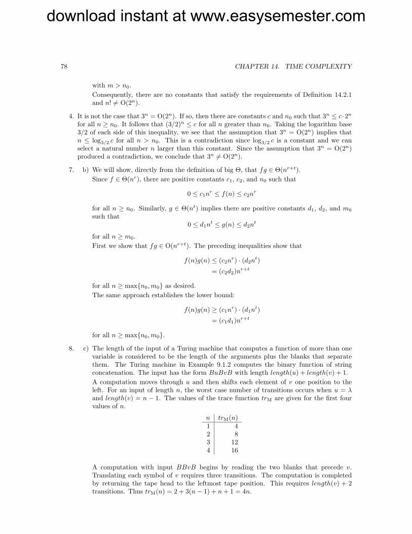
download instant at www.easysemester.com
78 CHAPTER 14. TIME COMPLEXITY
with m > n0.Consequently, there are no constants that satisfy the requirements of Definition 14.2.1and n! 6= O(2n).
4. It is not the case that 3n = O(2n). If so, then there are constants c and n0 such that 3n ≤ c ·2n
for all n ≥ n0. It follows that (3/2)n ≤ c for all n greater than n0. Taking the logarithm base3/2 of each side of this inequality, we see that the assumption that 3n = O(2n) implies thatn ≤ log3/2 c for all n > n0. This is a contradiction since log3/2 c is a constant and we canselect a natural number n larger than this constant. Since the assumption that 3n = O(2n)produced a contradiction, we conclude that 3n 6= O(2n).
7. b) We will show, directly from the definition of big Θ, that fg ∈ Θ(nr+t).Since f ∈ Θ(nr), there are positive constants c1, c2, and n0 such that
0 ≤ c1nr ≤ f(n) ≤ c2n
r
for all n ≥ n0. Similarly, g ∈ Θ(nt) implies there are positive constants d1, d2, and m0
such that0 ≤ d1n
t ≤ g(n) ≤ d2nt
for all n ≥ m0.First we show that fg ∈ O(nr+t). The preceding inequalities show that
f(n)g(n) ≤ (c2nr) · (d2n
t)
= (c2d2)nr+t
for all n ≥ max{n0, m0} as desired.The same approach establishes the lower bound:
f(n)g(n) ≥ (c1nr) · (d1n
t)
= (c1d1)nr+t
for all n ≥ max{n0, m0}.8. c) The length of the input of a Turing machine that computes a function of more than one
variable is considered to be the length of the arguments plus the blanks that separatethem. The Turing machine in Example 9.1.2 computes the binary function of stringconcatenation. The input has the form BuBvB with length length(u) + length(v) + 1.A computation moves through u and then shifts each element of v one position to theleft. For an input of length n, the worst case number of transitions occurs when u = λand length(v) = n − 1. The values of the trace function trM are given for the first fourvalues of n.
n trM(n)1 42 83 124 16
A computation with input BBvB begins by reading the two blanks that precede v.Translating each symbol of v requires three transitions. The computation is completedby returning the tape head to the leftmost tape position. This requires length(v) + 2transitions. Thus trM(n) = 2 + 3(n− 1) + n + 1 = 4n.

download instant at www.easysemester.com
SOLUTIONS TO EXERCISES 79
11. The computation of a standard machine that accepts the language L = {aibi | 0 ≤ i ≤50} ∪ {u | length(u) > 100} begins using 100 states to check the length of the input. If themachine has not encountered a blank after 100 transitions, the computation halts and acceptsthe input string.
If the machine reads a blank prior to reading 100 input symbols, the computation
1. moves the tape head to position 0, and
2. runs a machine from that accepts {aibi | i ≥ 0}.The latter step can be accomplished in (n+2)(n+1)/2 transitions for an input string of lengthn.
The maximum number of transitions in the entire computation for an input of length n is
tcM(n) ={
2n + 2 + (n + 2)(n + 1)/2, if n ≤ 100101, otherwise.
The asymptotic complexity of M is constant, tcM(n) = Θ(1), since the number of transitionsis constant as n approaches infinity.
13. A one-tape deterministic Turing machine can be designed to accept the language {aibi | i ≥ 0}in time O(n lg(n)) by marking half of the a’s and half of the b’s on each pass through the input.
The computation begins reading the input, marking every other a with an X, and recordingwhether the number of a’s was even or odd. Upon scanning a b, it is marked as well as everyother subsequent b. As with the a’s, the states are used to record parity of the number ofb’s read. If an a is encountered after the first b, the computation halts and rejects the input.Upon completing the scan of the input, the following halting conditions are checked:
(a) If no a’s and b’s were found, the string is accepted.
(b) If there were a’s but no b’s, the string is rejected.
(c) If there were b’s but no a’s, the string is rejected.
(d) If the parity of the number of a’s and b’s was different, the string is rejected.
If none of the halting conditions were triggered, tape head returns to tape position 0 to makeanother pass of the input. On this pass, the X’s are skipped while marking every other aand b. On the completion of the pass, the termination conditions are checked. The process isrepeated until one of the terminating conditions is satisfied.
The maximum number of transitions for a string of length n occurs with the input an/2bn/2 ifn is even and a(n+1)/2b(n−1)/2 if n is odd. Each iteration of the preceding cycle requires 2n+2transitions and the maximum number of iterations is dlg(n)e. Thus the maximum number oftransitions is (2n + 2)dlg(n)e.The number of transitions could be reduced by one-half if we marked symbols going bothleft-to-right and right-to-left. However, this would not alter the big oh evaluation of the timecomplexity.

download instant at www.easysemester.com
80 CHAPTER 14. TIME COMPLEXITY

download instant at www.easysemester.com
Chapter 15
P ,NP , and Cook’s Theorem
1. a) The computations for the string aa are
q0BaaB q0BaaB q0BaaB q0BaaB` Bq1aaB ` Bq1aaB ` Bq1aaB ` Bq1aaB` Baq1aB ` Baq1aB ` Baq1aB ` q2BaaB` Baaq1B ` Bq2aaB ` Bq2aaB
` q2BaaB ` Baq3aB` Baaq3B
b) The worst-case performance with input an occurs when the computation reads the firstn− 1 a’s in q1 and transitions to q2, stays in q2 and moves left until it reads the first a,then moves right in state q3 until the computation halts.
c) The time complexity is
tcM(n) ={
1, if n = 0;3n− 1, otherwise.
5. a) We will use a proof by contradiction to show that the language
L = {R(M)w | M accepts w using at most 2length(w) transitions}is not accepted by any deterministic polynomial-time Turing machine. The contradictionis obtained using diagonalization and self-reference.Assume that L is in P. Then L is also in P. Since L is in P, there is some Turing machineM′ that accepts it in polynomial time. The self-reference occurs in asking if R(M′)R(M′)is in L; that is, does M′ accept R(M′)?Consider the first possibility, that R(M′)R(M′) is in L. This means that M′ does not acceptR(M′) in 2length(R(M′)) steps. Thus either the computation takes more than 2R(M′
) orM′ does not accept R(M′). The first case indicates that the computations of M′ are notpolynomially bounded and the second case indicates that R(M′)R(M′) is not in L. Bothof these possibilities yield a contradiction.The second possibility is that R(M′)R(M′) is not in L. This means that M′ accepts R(M′)in at most 2length(R(M′)) transitions. Consequently R(M′)R(M′) is in L, a contradiction.Both possibilities, that R(M′)R(M′) is in L and R(M′)R(M′) is not in L, produce acontradiction. Thus our assumption could not be true and the language L is not in P.
81

download instant at www.easysemester.com
82 CHAPTER 15. P,NP, AND COOK’S THEOREM
9. Intuitively, the polynomial time bound p(n) can be used to terminate all computations of Mthat use more than p(n) transitions. To accomplish this, a machine M′ is constructed that hasone more tape than M, which we will call the counter tape. The computation of M′
1. Writes p(n) 1 ’s on the counter tape and repositions the tape head at the beginning ofthe string of 1 ’s.
2. While the counter tape head is reading a 1, M′
- Moves the counter tape head one position to the right.- If a transition of M is defined, then M′ simulates the transition on original tapes.
Otherwise M′ halts and returns the same result as M.
3. M′ halts and does not accept when a B is read on the counter tape.
For every string u ∈ L(M), there is at least computation that requires p(n) or fewer transitionsand accepts u. The simulation of this computation in M′ will also accept u. Clearly, L(M′) iscontained in L(M) since it only accepts strings that are accepted by M. Thus M′ accepts L(M)and halts for all input strings.
The computation of M′ for an input string u of length n consists of the writing p(n) 1 ’s on thecounter tape and simulating the computation of M. The number of transitions in the simulationis bounded by p(n) and writing p(n) 1 ’s can be accomplished in time polynomial in n.
10. b) The Turing machine M reduces the problem of recognizing the language L1 = {aibiaj |i, j ≥ 0} to that of recognizing L2 = {cidi | i ≥ 0}.
INSERT FIGURE 15.2 HERE
If the input string has the form aibkaj , the computation of M produces the string cidk.This string will be accepted by a machine that recognizes L2 only if i = k. Computationsof M with input that do not have the form aibkaj produce a string consisting solely ofc’s, which will be rejected by a machine that recognizes L2.
12. In the first printing of the book, the state diagram is incorrect. The arcs on the bottom shouldgo from right-to-left and there should be a transition B/B L on the arc from q6 to qf . Theanswers given are for the state diagram with these modifications.
a)
q0BabbaB ` #abq5bBB
` #q1abbaB ` #aq5bdBB
` #aq2bbaB ` #q5addBB
` #abq3baB ` q5#cddBB
` #abbq4aB ` Bq6cddBB
` #abbBq4B ` qfBcddBB
` #abbq5BB
b) Any string will cause the maximum number of transitions. The computation reads theentire string from left-to-right, then again from right-to-left, and ends with two transitionsto erase the endmarker.

download instant at www.easysemester.com
SOLUTIONS TO EXERCISES 83
c) tcM(n) = 2n + 4
d) The function computed by the machine is not a reduction of L to Q. The string ab ismapped to cd; the former is not in L while the latter is in Q.
15. Any combination of three of the clauses x, y, z, and ¬x ∨ ¬y ∨ ¬z is satisfiable. The fourclauses, however, are unsatisfiable. The satisfaction of the clause ¬x ∨ ¬y ∨ ¬z requires thetruth assignment for one of the Boolean variables to be 0. This precludes the clause thatconsists of that variable alone from being satisfied.
17. The assumption the P = NP is critical in the arguments that follow. Of course, we do notknow if this assumption is true.
a) Let L be a language in NP that is neither empty nor is its complement empty. Thatmeans that are strings u and v such that u ∈ L and v ∈ L.To prove that L is NP-complete, we must show that every language Q in NP is reducibleto L in polynomial time. Since NP = P, we know that there is a Turing machine M thataccepts Q in polynomial time. A polynomial time reduction of Q to L can be obtainedas follows: For a string w
1. Run M to determine if w ∈ Q.2. If w ∈ Q, then erase the tape and write u in the input position. Else erase the tape
and write v in the input position.
This is clearly a reduction of Q to L. Moreover, it can be accomplished in polynomialtime since the computation of Q is polynomial.
b) In part (a) we have shown that every language in NP other than ∅ and its complementis NP-complete. These languages clearly are in P = NP, but are not NP-complete. Tobe able to reduce a nonempty language Q to the ∅, we must map strings in Q to a stringin ∅ and strings not in Q to a string not in ∅. Unfortunately, we cannot do the formersince there are no strings in ∅.

download instant at www.easysemester.com
84 CHAPTER 15. P,NP, AND COOK’S THEOREM

download instant at www.easysemester.com
Chapter 16
NP-Complete Problems
1. A formula is in 2-conjunctive normal form if it is the conjunction of clauses each of which hastwo literals. The 2-Satisfiability Problem is to determine whether an arbitrary 2-conjunctivenormal form is satisfiable.
We will describe a polynomial-time algorithm that solves the 2-Satisfiability Problem. Thealgorithm constructs a truth assignment if the formula is satisfiable. If not, the attempt toconstruct the assignment fails.
Before outlining the strategy, we first note that the assignment of a truth value to a variablemay be used to reduce the length of a 2-conjunctive normal form formula that needs to beconsidered for determining satisfiability. Consider the formula
(x1 ∨ x2) ∧ (¬x2 ∨ ¬x3) ∧ (¬x1 ∨ x3) ∧ (x1 ∨ ¬x4).
If t(x1) = 1, then any clause that contains x1 can be deleted since it is satisfied by t. Thisproduces
(¬x2 ∨ ¬x3) ∧ (¬x1 ∨ x3).
Moreover, the occurrence of the literal ¬x1 can be deleted from clauses since its value will notsatisfy the clause. Applying this reduction yields
(¬x2 ∨ x3) ∧ (x3).
Since x3 occurs as a singleton, it is necessary to assign t(x3) = 1 to satisfy the formula. Doingthe reduction produces
(¬x2).
The only truth assignment that satisfies this clause is t(x2) = 0.
In this example, we set t(x1) = 1 and reduced based on this truth assignment. When all clausesare removed following the preceding rules, we have succeeded in constructing a satisfying truthassignment. In the preceding reduction, no value has been assigned to the variable x4. Thisindicates that the value assigned to x4 is irrelevant; either choice will yield an assignment thatsatisfies the formula.
Before describing the algorithm in detail, let us consider two more examples; one which failsto find a satisfying truth assignment and one which requires several steps to complete. Weattempt to find a satisfying truth assignment for
(x1 ∨ x2) ∧ (¬x1 ∨ ¬x2) ∧ (¬x1 ∨ ¬x3) ∧ (x2 ∨ x3).
85

download instant at www.easysemester.com
86 CHAPTER 16. NP-COMPLETE PROBLEMS
Setting t(x1) = 1 yields(¬x2) ∧ (¬x3) ∧ (x2 ∨ x3).
Reducing by setting t(x2) = 0 produces the contradictory clauses
(¬x3) ∧ (x3).
The reduction fails because there is no assignment that can satisfy both of these clauses. Atthis point we conclude that there is no satisfying truth assignment that can be obtained bysetting t(x1) to 1. The next step would be to begin the process by setting t(x1) = 0 and tryingto find a satisfying truth assignment with this assignment to x1.
Our final example illustrates the need to select the truth value for more than one variable toproduce a satisfying assignment. The result of assigning t(x1) = 1 in
(x1 ∨ x2) ∧ (¬x1 ∨ x3) ∧ (¬x3 ∨ x2) ∧ (x4 ∨ x5)
produces(x3) ∧ (¬x3 ∨ x2) ∧ (x4 ∨ x5),
requiring t(x3) = 1 in order to satisfy the formula. The effect of this assignment yields
(x2) ∧ (x4 ∨ x5),
which requires t(x2) = 1 in a satisfying truth assignment. The resulting formula
(x4 ∨ x5),
matches neither of the termination conditions; the formula is not empty and it does not containcontradictory clauses. We continue the process by selecting a truth assignment for one of thevariables in (x4 ∨ x5) and applying the reduction procedure.
Each reduction process is initiated with the selection of a truth assignment for a variable xi.If the reduction does not produce contradictory clauses, this truth assignment, along with ofthose obtained during the reduction, are incorporated into the final truth assignment.
To describe the algorithm we let u = w1 ∧ · · · ∧ wm be a 2-conjunctive normal form formulaand V = {x1, . . . , xn} be the set of variables of u. The objective is to build a satisfying truthassignment t on V. For a formula v, we use the reduction procedure to build a truth assignmentT on the set of variables in v, denoted var(v). If the reduction does not fail, we then assignthe truth values of T to t.
The algorithm proceeds as follows:
1. Let v = u.
2. Set T (x) ↑ for all x ∈ var(v), and pick a variable xi in var(v).
3. Set T (xi) = 1 and reduce v.
4. If the reduction did not fail and produced the formula v′, then
- Set t(x) = T (x) for all x ∈ var(v) for which T (x) is defined.- If v′ is empty, continue with step 8,- otherwise set v = v′ and continue with step 2.
5. The reduction for T (xi) = 1 has failed. Set T (xi) = 0 and reduce v.
6. If the reduction did not fail and produced the formula v′, then
- Set t(x) = T (x) for all x ∈ var(v) for which T (x) is defined.

download instant at www.easysemester.com
SOLUTIONS TO EXERCISES 87
- If v′ is empty, continue with step 8,- otherwise set v = v′ and continue with step 2.
7. If both reductions failed, the formula is unsatisfiable.8. For each xj with t(xj) ↑, select any truth value for t(xj). The truth assignment t satisfies
u.
The truth assignment t clearly satisfies u, since the reduction removes a clause only when ithas been satisfied. Moreover, the algorithm will produce a truth assignment whenever u issatisfiable. Assume that u is satisfied by some truth assignment t′. The selection of truth valuesT (xi) = t′(xi) in steps 3, 5, and 7 will produce the truth assignment t = t′. Consequently, weare assured of the construction of some truth assignment whenever u is satisfiable.
Once a variable is assigned a truth value in step 4 or 6, that value does not change. At most2n reductions are possible and each reduction can alter at most m clauses. Thus the algorithmcompletes in time polynomial to the number of variables and clauses in the formula.
6. A guess-and-check strategy that yields a nondeterministic polynomial time solution to theminimum set cover problem is straightforward. The guess nondeterministically selects a sub-collection C′ of C of size k. The check verifies that every element in S is in the union of thesets in C′.We show that the Minimum Set Cover Problem is NP-hard by reducing the 3-SatisfiabilityProblem to it. First we will outline the construction of a set S, a collection C of subsets ofS, and a number k from a 3-conjunctive normal form formula u. We will then show that S iscovered by k sets in C if, and only if, u is satisfiable.
To accomplish the reduction, we must reformulate truth assignments and clauses in terms ofsets. Let
u = w1 ∧ · · · ∧ wm
= (u1,1 ∨ u1,2 ∨ u1,3) ∧ · · · ∧ (um,1 ∨ um,2 ∨ um,3)
be a 3-conjunctive normal form formula with m clauses. The variables of u are {x1, . . . , xn}and the symbol uj,k represents the kth literal in clause wj .
We will construct the elements of S and the sets of C in three steps. The sets are built so thatthe smallest cover C′ of S consists of 2mn sets from C. We begin with the sets that representtruth assignments. For each variable xi, construct the sets
{¬xi,1, ai,1, bi,1}{xi,1, ai,2, bi,1}{¬xi,2, ai,2, bi,2}{xi,2, ai,3, bi,2}{¬xi,3, ai,3, bi,3}{xi,3, ai,4, bi,3}
...{¬xi,m, ai,m, bi,m}{xi,m, ai,1, bi,m}
There are 2mn sets of this form, 2m for each variable xi. The elements xi,j ,¬xi,j , i = 1, . . . , nand j = 1, . . . , m, and ai,1, . . . , ai,m and bi,1, . . . , bi,m, i = 1, . . . , n are added to the set S.

download instant at www.easysemester.com
88 CHAPTER 16. NP-COMPLETE PROBLEMS
The preceding sets are the only sets of C that contain the elements ai,1, . . . , ai,m and bi,1, . . . , bi,m.For a fixed variable i, we can cover ai,1, . . . , ai,m and bi,1, . . . , bi,m with m of these sets. Thisis possible only if we choose all the sets that contain ¬xi,k or all of the sets that contain xi,k.
This choice provides our intuition for a truth assignment. If the cover contains all the sets with¬xi,k, we associate this with a truth assignment that assigns 1 to xi,k. In a like manner, if thecover contains all the sets with xi,k, we associate this with a truth assignment that assigns 0to xi,k.
Now we add elements and sets used to represent the clauses of u. For each clause wj ,
- If the literal xi occurs in wj , then construct set {xi,j , s1,j , s2,j}.- If the literal ¬xi occurs in wj , then construct set {¬xi,j , s1,j , s2,j}.
These are the only sets of C that contain s1,j and s2,j . Thus at least one of the three setsgenerated from wj is required for any cover of S.
To this point, the cover that we are building requires mn + m sets: mn from the truth settingsets and m from the clause sets. Each of the ai,j ’s, bi,j ’s, s1,j ’s, and s2,j are covered by such aselection. If the sets from the truth setting component for a variable xi all contain ¬xi,j , thenthe xi,j ’s are not covered. Similarly, if the sets from the truth setting component all containxi,j , then the ¬xi,j ’s are not covered. We must add more sets so that these elements will becovered. We will refer to these sets as the completion sets, since they complete the coverageof the xi,j ’s or ¬xi,j ’s
For each variable xi and clause wj , we add the sets
{¬xi,j , c1,k, c2,k}{xi,j , c1,k, c2,k}
for k = 1, . . . , m(n− 1). The elements c1,k and c2,k appear only in these sets. Thus m(n− 1)completion sets are necessary to cover the c’s
This completes the construction of S and C from u. From the form of the sets, we see that acover of S must contain at least 2mn sets from C. We now must show that u is satisfiable if,and only if, there are 2mn sets in C that cover S.
If u is satisfied by a truth assignment t, we can build a cover of S consisting of 2mn sets asfollows. For each variable xi,
- If t(xi) = 1, then add the mn sets of the form {¬xi,1, ai,k, bi,k} to C′.- Otherwise add the sets {xi,1, ai,k, bi,k} to C′.
Each clause wj is satisfied by at least one literal. For one of the satisfying literals we will add aclause set to C′. If t(xi) = 1 and xi is in wj , then add the set {xi,j , s1,j , s2,j} to C′. If t(xi) = 0and ¬xi is in wj , then add {¬xi,j , s1,j , s2,j} to C′. In either case, this set covers s1,j and s2,j
and adds one set to C′.For a clause wj that was satisfied by a positive literal xi in the preceding step, the elementsxt,j , where t 6= i, are not covered by our sets. These are covered by the addition of the m− 1completion sets
{xt,j , c1,k, c2,k},where t 6= i and a different k is selected for each set. These m−1 sets simultaneously completethe coverage of the xt,j ’s and the c1,k’s and c2,k’s.

download instant at www.easysemester.com
SOLUTIONS TO EXERCISES 89
Similarly, for a clause wj that was satisfied by a negative literal ¬xi, the elements ¬xt,j , wheret 6= i, are not covered by the truth setting or clause sets. These are covered by the addition ofthe m− 1 sets of the form
{¬xt,j , c1,k, c2,k},where t 6= i.
Thus we have a total of mn truth setting sets, m clause sets, and m(n− 1) completion sets fora cover of S by 2mn sets.
Conversely, if S is covered by 2mn sets from C′. The cover must consist of mn truth settingsets, m linking sets, and m(n − 1) of the completion sets. We can obtain a truth assignmentfrom the truth setting sets in C′. If the sets {xi,1, ai,k, bi,k} are in the cover, then t(xi) = 0;otherwise, t(xi) = 1.
For each clause wj , one set of the form {xi,j , s1,j , s2,j} or {¬xi,j , s1,j , s2,j} is in the cover. Inthe former case, the xi satisfies wj . In the latter case, the ¬xi is satisfies wj .
8. We will show that the Longest Path Problem is NP-hard by reducing the Hamiltonian CircuitProblem to it. The transformation converts a graph G = (N, A) into a graph G′ = (N′, A′)in two steps.
We construct G′ from G by adding three nodes and the arcs incident to these nodes. Let N= {v1, . . . , vn} be the set of nodes of G. First we make a copy v′1 of v1. For each arc [vi, v1] inA, vi 6= v1, add an arc [vi, v
′1] as illustrated in the diagram below.
INSERT FIGURE Chapter 16 exercise 9 HERE
The construction of G′ is completed by adding nodes x and y and arcs [x, v1] and [v′1, y]. Thereduction is complete by selecting the number k = n + 2 as the input in the Longest PathProblem.
To show that the preceding construction is a reduction, we must show that G has a tour if,and only if, G′ has an acyclic path of length n + 2.
Assume that G has a tour. The tour can be written as a path v1, vi2 , . . . , vin , v1 of length n.Replacing the v1 at the end of the path with v′1 and adding the arcs [x, v1] and [v′1, y] createsan acyclic path of length n + 2 in G′.
Now assume that G′ has an acyclic path of length n + 2. Since G′ has n + 3 nodes, this pathmust visit every node. To reach nodes x and y, the path must begin with the arc [x, v1] andend with [v′1, y]. Deleting these produces an acyclic path with endpoints v1 and v′1. Equatingv1 and v′1 produces a tour v1, vi2 , . . . , vin , v1 in G.
9. a) The Multiprocessor Scheduling Problem can be converted into a decision problem byadding a deadline for the computations as follows:Input: set of tasks A,
length of task function l : A → Nnumber of processors k, anddeadline m
Output: yes, if there is a partition A1, . . . , Ak suchthat l(Ai) ≤ m for all i,
no, otherwise.With the deadline, the problem is to determine if there an assignment of tasks to proces-sors that ensures that all tasks will be completed by time m.

download instant at www.easysemester.com
90 CHAPTER 16. NP-COMPLETE PROBLEMS
b) Following the strategy employed in the proof of the NP-completeness of the Bin PackingProblem, we will reduce the Partition Problem to the Multiprocessor Scheduling Problem.The reduction transforms an instance of the Partition Problem into an instance of theMultiprocessor Scheduling Problem. The transformation is accomplished by the mapping
Partition MultiprocessorScheduling
Set A AFunction v l = vNumber of sets k = 2Bound m = v(A)/2
Now we must show that an instance (A, v) of the Partition Problem has a solution if, andonly if, the corresponding instance (A, l, k, m) of the Multiprocessor Scheduling Problemhas a solution.Assume that there is a subset A′ ⊆ A such that v(A′) = v(A)/2. Then the partitionA1 = A′, A2 = A − A′ is a solution to the corresponding Multiprocessor SchedulingProblem.Conversely, assume that the Multiprocessor Scheduling Problem has a solution A1 andA2. Since A = A1∪A2, l(A) = l(A1)+ l(A2). However, satisfaction of the deadline boundensures us that l(A1) ≤ l(A)/2 and l(A2) ≤ l(A)/2. It follows that l(A1) = l(A2) = l(A)/2and A1 is a solution to the Partition Problem.
10. To show that the Integer Linear Programming Problem is NP-hard, we reduce the questionof the satisfiability of a 3-conjunctive normal form formula to that of satisfying a system ofintegral inequalities. Let
u = w1 ∧ w2 ∧ · · · ∧ wm
be a 3-conjunctive normal form formula with clauses wi = ui,1 ∨ ui,2 ∨ ui,3 and let V ={x1, x2, . . . , xn} be the set of Boolean variables occurring in w.
We will consider the literals as variables that may assume integer values. For each pair ofliterals xi and ¬xi in V, the four equations
1. xi ≥ 02. ¬xi ≥ 03. xi + ¬xi ≥ 14. −xi − ¬xi ≥ −1
are satisfied only if one of xi and ¬xi is one and the other is 0. A set of inequalities 1–4) isconstructed for each variable xi in V. Satisfying the 4n inequalities defines a truth assignmentfor V. For each clause wi in u, we define the inequality
5. ui,1 + ui,2 + ui,3 ≥ 1,
where ui,j is the literal in the jth position of clause i. This inequality is satisfied only if oneof the literals in the clause is satisfied.
An integer linear programming system Ax ≥ b can be constructed from the 4 · n inequalitieswhose satisfaction defines a truth assignment for the variables of V and the m inequalities therepresent the clauses. The matrix A has a column for each literal xi and its negation ¬xi. Arow of A consists of the coefficients of the left-hand side of one of the 4 · n + m inequalities.The column vector b is obtained from the right-hand side of the inequalities. The system Ax≥ b is solvable if, and only if, the solution vector x defines a truth assignment that satisfies u.Clearly, a representation of A and b can be constructed in polynomial time from the clause u.Thus the Integer Linear Programming Problem is NP-hard.

download instant at www.easysemester.com
SOLUTIONS TO EXERCISES 91
13. Consider an instance of the Bin Packing Problem with items A = {a1, . . . , an}, size functions, and bin size m with the optimal number of bins denoted b∗. We will show that the first-fitalgorithm generates a packing which requires at most 2b∗ bins.
Let
T =n∑
i=1
s(ai),
be the total size of the items in the set A. T can be used to obtain lower bound on the numberof bins in the optimal solution:
b∗ ≥ dT/me.
First we note that at the completion of the first-fit algorithm, there is at most one bin that isless than half full. If a packing produces two bins numbered r and s that are both less thanhalf full, then that packing could not have been produced by the first-fit algorithm. Assumethat packing bin r occurred before packing bin s. When encountering the items in bin s, thefirst-fit algorithm would have placed these items into bin r. Thus whatever strategy was usedto assign the items, it was not the first-fit algorithm.
Now assume that d2T/me+ 1 or more bins are used in the first-fit packing. By the argumentin the preceding paragraph, at least d2T/me are more than half full. Thus the total size of thecontents is greater than
m/2d2T/me ≥ T,
which is a contradiction since T is the sum of the size of all the ai’s.
Thus we conclude that at most d2T/me = 2dT/me = 2b∗ are required in the solution producedby the first-fit algorithm.
15. We will show that the modification to the greedy algorithm produces a 2-approximation algo-rithm for the Knapsack Problem. Let S = {a1, . . . , an} be the set of objects, b the size bound,and s : S → N and v : S → N be the size and value functions, respectively. Also let c∗ be thevalue of the optimal solution and cg be the value produced by the greedy algorithm.
We assume that the items have been sorted by relative value,
v(a1)/s(a1) ≥ v(a2)/s(a2) ≥ · · · ≥ v(an)/s(an),
as required by the greedy algorithm and that every item in the list has size at most b. Anyitem with size greater than b can be removed from consideration since it cannot appear in asolution.
If all the items fit into the knapsack, then the optimal solution consists of all the items in Sand this solution is discovered by the greedy algorithm.
Now we consider the case wheren∑
i=1
s(ai) ≥ b.
Let ak be the first item not able to be put into the knapsack by the greedy algorithm. Then
k−1∑
i=1
v(ai) ≤ cg ≤ c∗.
The elements a1, a2, . . ., ak provide an optimal solution for a Knapsack Problem with the sameset S but having size bound b′ =
∑ki=1 s(ai). The total value for this problem is
∑ki=1 v(ai) =

download instant at www.easysemester.com
92 CHAPTER 16. NP-COMPLETE PROBLEMS
c′. Now c∗ ≤ c′ since any set of items that can be packed into a knapsack with size bound bcan also be packed into the larger knapsack with size bound b′.
Let a∗ denote the item that has the largest value in S. Since a∗ has the maximum value ofany item in S, it follows that v(a∗) ≥ v(ak). Combining the inequalities, v(a∗) ≥ v(ak) and∑k−1
i=1 v(ai) ≤ cg we get
max{v(a∗), cg}
≥ max{v(ak),
k−1∑
i=1
v(ai)}
≥ (v(ak) +
k−1∑
i=1
v(ai))/2
≥ ( k∑
i=1
v(ai))/2
≥ c′/2≥ c∗/2
as desired. The third step follows from the inequality
max{x, y} ≥ (x + y)/2
that compares the maximum and the average of two numbers.

download instant at www.easysemester.com
Chapter 17
Additional Complexity Classes
2. A three-tape Turing machine can be designed to accept the language {aibi | i ≥ 0} in loga-rithmic space. The input is on tape 1 and tapes 2 and 3 serve as counters. Using the binaryrepresentation, the number of a’s that have been read is recorded on tape 2 and the num-ber of b’s on tape three. A computation consists of two steps: accumulating the counts andcomparing the results. The machine accepting {aibi | i ≥ 0}
1. Reads the input on tape 1 and
- If an a is read after a b, the computation halts and rejects the input.- On reading an a, the counter on tape 2 is incremented.- On reading a b, the counter on tape 3 is incremented.
2. After processing the input, the strings on tapes 2 and 3 are compared.
- If the strings are identical, the input is accepted.- Otherwise, it is rejected.
The worst case performance for a string of length n occurs with the input string an. In thiscase, the counter on tape 2 uses dlg(n)e+ 1 tape squares.
3. The tape bound limits the number of configurations that can occur in an accepting computa-tion. By Corollary 17.3.3, we know that the number of transitions is bounded by cs(n), wherec is determined by the number of states and tape symbols of M.
The strategy of employing a counter tape to terminate computations in which the number oftransitions exceeds the bound can be used to construct a Turing machine M′ that accepts Land halts for all inputs. This strategy was described in the solution to Exercise 9 in Chapter15. The machine M′ is no longer subject to the space bound, but it does demonstrate that Lis recursive.
7. We sketch the design of a one-tape deterministic machine M for which every computation withinput of length n > 1 reads exactly 2n tape squares. The input alphabet for M is {a}.For an input string an, the computation begins with tape configuration BanB. The computa-tion begins by writing a # in tape position 0 and reading the input. If the input string haslength 0, 1, or 2. The computation terminates after reading the entire input string. For inputof length 2, the computation reads the initial blank, the input aa, and the following blankusing 4 tape squares as required.
For computations with input an, n > 2, we construct a loop that iteratively doubles the lengthof a string produced on previous iteration. The objective is to construct a string of length 2n
93

download instant at www.easysemester.com
94 CHAPTER 17. ADDITIONAL COMPLEXITY CLASSES
on the tape beginning at position 0. Since this string must overwrite the input string, we willuse the additional tape symbols to differentiate the input from the generated string.
The string beginning at position 0 that has length 4, 8, 16, and so forth will consist of #, b’s,c’s and X’s and be referred to as the generated string. Each time we double the generatedstring, we will mark one input symbol as processed. The c’s represent unprocessed input thatare already in the generated string and the a’s represent unprocessed whose tape positionshave not already been incorporated into the string. After all the a’s have been changed to b’sor c’s, the generated string is expanded by adding X’s.
The computation will halt when all the input symbols have been processed. The meaningsassociated with the tape symbols are
# left tape boundary markera, a′ unprocessed input symbolc, c′ unprocessed input symbol in the generated stringb, b′ processed input symbolX, X ′ elements added to the generated string beyond the n− 1st
tape positionY elements used in the copying
The symbols with primes are used in the extension of the generated string.
As previously noted, the computation begins by writing a # in tape position 0 and readingthe input. For input of length greater than 2, the final a is erased and the head returns totape position 0. The first a in the input is then changed to b and the second a is changed to ac. If the next symbol is blank, an X is written. Otherwise, the next a is also changed to a c.This produces the tape configuration #bcX for an input string of length 3 and #bccan−4 foran input of length 4 or more.
The # and b indicate that two symbols have been processed and the length of the generatedstring is 4.
The loop that generates the string proceeds as follows:
(a) The tape head moves to the right to find an a or c. If none is found, the computationhalts.
(b) The tape head returns to position 0.
(c) One symbol at a time, each symbol b, c, X in the generated string is replaced by a b′, c′,X ′ and a symbol is added to the end of the generated string.
- If an a is encountered, it is changed to an a′.- If a blank is encountered, it is changed you Y .
(d) After writing the final Y or a′, the tape head returns to position 0. On this pass it changesY and X ′ to X, a′ and c′ to c, and b′ to b.
(e) The first occurrence of an a or c is changed to a b.
(f) The tape head returns to position 0 and the computation continues with step a).
For example, for input aaaaa, the tape configurations at the beginning of each loop are
#bccaBBBBBBBBBBBB16
#bbccXXXBBBBBBBBB16
#bbbcXXXXXXXXXXXB16
#bbbbXXXXXXXXXXXX16

download instant at www.easysemester.com
SOLUTIONS TO EXERCISES 95
12. Doubling the amount of available tape does not change the set of languages that can beaccepted. We show that a language accepted by a Turing machine M whose computationsrequire at most 2s(n) tape squares can also be accepted by Turing machine M′ with tapebound s(n). By Theorem 17.2.2, we can restrict our attention to Turing machines with onework tape.
Let M = (Q, Σ, Γ, δ, q0, F) be a Turing machine whose computation have a 2s(n) tape bound.The input and tape alphabets Σ′ and Γ′ of M′ are
Σ′ = Σ, andΓ′ = {B} ∪ (Γ× Γ× {1, 2}).
Since M′ is designed to accept L(M), the input alphabets of M and M′ are identical. Thetape alphabet of M′ has triples [x, y, i] with x, y ∈ Γ and i ∈ {1, 2}. The reduction in amountof tape required by the computations of M′ is achieved by the storing more information in asingle tape symbol; a tape symbol of M′ contains two symbols from M. The integer value inthe ordered triple indicates which of the two symbols from Γ would be scanned by M.
When M′ reads a B on the work tape, M′ interprets the blank as the triple [B, B, 1] andthe transition converts it into a triple. The transition function δ′ of M′ is obtained from thetransition function δ of M as follows:
Transition of M Transitions of M′
δ(qi, a, x) = [qj ; b, d; z,R] δ′(qi, a, [x, y, 1]) = [qj ; b, d; [z, y, 2], S]δ′(qi, a, [y, x, 2]) = [qj ; b, d; [y, z, 2], R]
δ(qi, a, x) = [qj ; b, d; z, L] δ′(qi, a, [x, y, 1]) = [qj ; a, d; [z, y, 1], L]δ′(qi, a, [y, x, 2]) = [qj ; b, d; [y, z, 1], S]
δ(qi, a, B) = [qj ; b, d; z,R] δ′(qi, a, B) = [qj ; b, d; [z,B, 2], S]
δ(qi, a, B) = [qj ; b, d; z, L] δ′(qi, a, B) = [qj ; b, d; [z,B, 1], L]
where x, y, z are elements of Γ, d ∈ {L, R}, and S indicates that the tape head remainsstationary in the transition.
The computation of M′ with an input string u simulates that of M with u but reads at mosts(n) tape squares on the work tape.
15. The NP-hardness of a P-space complete language follows directly from the definition of P-Space and the inclusions shown in Figure 17.4. Let Q be a P-Space complete language. Thismeans that Q is in P-Space and that every language in P-Space is reducible to Q in polynomialtime. Since NP is a subset of P-space, it follows that every language in NP is reducible to Qin polynomial time and, consequently, Q is NP-hard.

download instant at www.easysemester.com
96 CHAPTER 17. ADDITIONAL COMPLEXITY CLASSES

download instant at www.easysemester.com
Chapter 18
Parsing: An Introduction
2. The subgraph of the graph of the grammar G consisting of all leftmost derivations of lengththree or less is
INSERT FIGURE Chapter 18 Exercise 2 HERE
5. The search tree created by Algorithm 18.2.1 while parsing ((b)) is given below. The nodes oneach level are listed in the order of their generation.
INSERT FIGURE 4.17 HERE
The derivation of ((b)) is obtained by following the arcs from the root S to the goal node ((b)).
Derivation Rule
S ⇒ A S → A⇒ T A → T⇒ (A) T → (A)⇒ (T ) A → T⇒ ((A)) T → (A)⇒ ((T )) A → T⇒ ((b)) T → b
11. Algorithm 18.4.1 will not terminate when run with input string aa and grammar
S → A | a | aaA → S
The rule S → a establishes Sa as the result of the first reduction for the string aa. The parseproceeds by alternating reductions with the rule A → S and the rule S → A.
97

download instant at www.easysemester.com
98 CHAPTER 18. PARSING: AN INTRODUCTION

download instant at www.easysemester.com
Chapter 19
LL(k) Grammars
2. a) The lookahead sets are given for the rules of the grammar. The lookahead set for avariable A is the union of the lookahead sets of the A rules.
Rule Lookahead setS → ABab {abab, acab, aab, cbab, ccab, cab}S → bAcc {bacc, bccc}A → a {abab, acab, aab, acc}A → c {cbab, ccab, cab, ccc}B → b {bab}B → c {cab}B → λ {ab}
3. b) The FIRST1 and FOLLOW1 sets for the variables of the grammar are
Variable FIRST1 FOLLOW1
S a, # λA a a, #B a #
To determine whether the grammar is LL(1), the techniques outlined in Theorem 19.2.5are used to construct the lookahead sets from the FIRST1 and FOLLOW1 sets.
Rule Lookahead setS → AB# {a, #}A → aAb {a}A → B {a, #}B → aBc {a}B → λ {#}
Since the lookahead sets for the alternative A rules both contain the symbol a, the gram-mar is not strong LL(1).
6. a) Algorithm 19.4.1 is used to construct the FIRST2 sets for each of the variables of thegrammar
S → ABC###A → aA | a
B → bB | λ
C → cC | a | b | c.
99

download instant at www.easysemester.com
100 CHAPTER 19. LL(K) GRAMMARS
The rules of the grammar produce the following assignment statements for step 3.2 of thealgorithm.
F (S) := F (S) ∪ trunc2(F ′(A)F ′(B)F ′(C){cc})F (A) := F (A) ∪ trunc2({a}F ′(A)) ∪ {a})F (B) := F (B) ∪ trunc2({b}F ′(B))F (C) := F (C) ∪ trunc2({c}F ′(C)) ∪ {a, b, c}
The algorithm is traced by exhibiting the sets produced after each iteration.
Step F (S) F (A) F (B) F (C)0 ∅ ∅ {λ} ∅1 ∅ {a} {λ, b} {a, b, c}2 {aa, ab, ac} {a, aa} {λ, b, bb} {a, b, c, ca, cb, cc}3 {aa, ab, ac} {a, aa} {λ, b, bb} {a, b, c, ca, cb, cc}
The rules that contain a variable on the right-hand side generate the assignment state-ments used in steps 3.2.2 and 3.2.3 of Algorithm 18.5.1. The rules S → ABC##,B → bB, and C → cC produce
FL(C) := FL(C) ∪ trunc2({##}FL′(S))= FL(C) ∪ {##}
FL(B) := FL(B) ∪ trunc2(FIRST2(C){##}FL′(S))= FL(B) ∪ {a#, b#, c#, ca, cb, cc}
FL(A) := FL(A) ∪ trunc2(FIRST2(B)FIRST2(C){##}FL′(S))= FL(A) ∪ {a#, b#, c#, ba, bb, bc}
FL(B) := FL(B) ∪ FL′(B)
FL(C) := FL(C) ∪ FL′(C)
The last two assignment statements may be omitted from consideration since they do notcontribute to the generation of FL(B) and FL(C).
Step FL(S) FL(A) FL(B) FL(C)0 {λ} ∅ ∅ ∅1 {a#, b#, c#, ba, bb, bc} {a#, b#, c#, ca, cb, cc} {##} ∅2 {a#, b#, c#, ba, bb, bc} {a#, b#, c#, ca, cb, cc} {##} ∅
The length two lookahead sets are used to construct the FIRST2 and FOLLOW2 sets.
Rule Lookahead setS → ABC## {aa, ab, ac}A → aA {aa}A → a {aa, ab, ac}B → bB {ba, bb, bc}B → λ {a#, b#, c#, ca, cb, cc}C → cC {ca, cb, cc}C → a {a#}C → b {b#}C → c {c#}

download instant at www.easysemester.com
SOLUTIONS TO EXERCISES 101
The lookahead sets of the A rules show that the grammar is not strong LL(2).
7. To establish part (3) of Lemma 19.2.2, we must show that the identity
FIRSTk(au) = {av | v ∈ FIRSTk−1(u)}
holds for all k ≥ 1. For convenience we let FIRST0(u) = {λ} for all strings u. Let v ∈FIRSTk−1(u) for some k ≥ 1. This implies that there is a derivation u
∗⇒ vx where vx ∈ Σ∗,length(v) = k − 1 or length(v) < k − 1 and x = λ. Consequently, au
∗⇒ avx and av is inFIRSTk(au).
The preceding argument shows that FIRSTk(au) ⊆ {a}FIRSTk−1(u). We must now establishthe opposite inclusion. Let av ∈ FIRSTk−1(au). Then au
∗⇒ avx where length(v) = k − 1 orlength(v) < k − 1 and xλ. The derivation u
∗⇒ vx, obtained by deleting the leading a fromthe preceding derivation, shows that v ∈ FIRSTk(u).
8. We will use a proof by contradiction to show every LL(k) grammar is unambiguous. Let Gbe an LL(k) grammar and assume that G is ambiguous. Then there is some string z that hastwo distinct leftmost derivations. Let S
∗⇒ uAv, u ∈ Σ∗, be the initial subderivation that isidentical in both derivations of z. The two derivations can be written
1)S∗⇒ uAv
∗⇒ ux1v∗⇒ uw = z
2)S∗⇒ uAv
∗⇒ ux2v∗⇒ uw = z.
The derivations continue by applying rules A → x1 and A → x2 to the variable A.
These derivations show that the string trunck(w) is in both LAk(uAv, A → x1) and LAk(uAv, A →x2). This is a contradiction; the sets LAk(uAv, A → x1) and LAk(uAv, A → x2) are disjointsince G is an LL(k) grammar. Thus our assumption, that G is ambiguous, must be false.
The exercise asked us to show that every strong LL(k) grammar is unambiguous. This followsimmediately since the strong LL(k) grammars are a subfamily of the LL(k) grammars.
9. a) The lookahead sets for the rules of G1 are
Rule Lookahead setS → aSb {ajaicibj | j > 0, i ≥ 0}S → A {aici | i ≥ 0}A → aAc {aici | i > 0}A → λ {λ}
For any k > 0, the string ak is a lookahead string for both of the S rules. Thus G1 is notstrong LL(k).A pushdown automaton that accepts L(G1) is defined by the following transitions.
δ(q0, a, λ) = [q1, A]δ(q1, a, λ) = [q1, A]δ(q1, b, A) = [q2, λ]δ(q1, c, A) = [q3, λ]δ(q2, b, A) = [q2, λ]δ(q3, b, A) = [q2, λ]δ(q3, c, A) = [q3, λ]
States q0 and q1 read an a and push A onto the stack. State q3 reads the c’s and q2 theb’s with each transition popping the stack. The accepting states are q0 and q2.

download instant at www.easysemester.com
102 CHAPTER 19. LL(K) GRAMMARS
11. a) The process of transforming the grammar into an equivalent strong LL(1) grammar beginsby removing the directly left recursive A rules, producing
S → A#A → aB | ZaBB → bBc | λZ → bZ | cZ | b | c
The resulting grammar is not strong LL(1) since there are two Z rules that begin with band two that begin with c. Left factoring these rules we obtain
S → A#A → aB | ZaBB → bBc | λZ → bX | cYX → Z | λY → Z | λ
Examining the length one lookahead sets, we see that this grammar is strong LL(1).
Rule Lookahead setS → A# {a, b, c}A → ab {a}A → Zab {b, c}B → bBc {b}B → λ {#}Z → bX {b}Z → cY {c}X → Z {b, c}X → λ {a}Y → Z {b, c}Y → λ {a}
13. a) The lookahead sets for the grammar G
S → aAcaa | bAbcc
A → a | ab | λ
are
Rule Lookahead setS → aAcaa {aacaa, aabcaa, acaa}S → bAbcc {babcc, babbcc, bbcc}A → a {acaa, abcc}A → ab {abcaa, abbcc}A → λ {caa, bcc}
One symbol lookahead is sufficient to discriminate between the S rules. Four symbols arerequired to choose the appropriate A rule. Thus G is strong LL(4).To show that G is LL(3), the lookahead sets are constructed for the sentential forms ofthe grammar.
Rule Sentential form Lookahead setS → aAcaa S {aaccaa, aabcaa, acaa}

download instant at www.easysemester.com
SOLUTIONS TO EXERCISES 103
S → bAbcc S {babcc, babbcc, bbcc}
A → a aAcaa {acaa}A → ab aAcaa {abcaa}A → λ aAcaa {caa}
A → a bAbcc {abcc}A → ab bAbcc {abbcc}A → λ bAbcc {bcc}
14. For every i > 0, the string ai is a prefix of both ai and aibi.
A nondeterministic pushdown automaton that accepts {ai | i ≥ 0} ∪ {aibi | i ≥ 0} was givenin Example 7.1.2. A deterministic automaton reads leading a’s and pushes an A on the stackin state q0 until either a blank or a b is read. If a blank is read, the stack is popped and thestring is accepted. If a b is read, a loop is entered that compares the number of b’s with thenumber of A’s stored on the stack. The pushdown automaton defined by the transitions
δ(q0, a, λ) = {[q0, A]}δ(q0, B, λ) = {[q1, λ]}δ(q0, b, A) = {[q2, λ]}δ(q1, λ, A) = {[q1, λ]}δ(q2, b, A) = {[q2, λ}
with accepting states q1 and q2 accepts the language.
15. It follows immediately from the definitions of LL(1) and strong LL(1) grammars that a strongLL(1) grammar G is also LL(1). To conclude that these families of grammars are identical, wemust show that every LL(1) grammar is also strong LL(1).
Let G = (V, Σ, S, P) be an LL(1) grammar and assume that it is not strong LL(1). Since Gis not strong LL(1), there are derivations
S∗⇒ u1Az1 ⇒ u1xz1
∗⇒ u1v1z1∗⇒ u1v1w1
S∗⇒ u2Az2 ⇒ u2yz2
∗⇒ u2v2z2∗⇒ u2v2w2
where
a) ui, vi, and wi are in Σ∗, zi ∈ (Σ ∪V)∗,
b) u1v1w1 6= u2v2w2,
c) A → x and A → y are distinct rules of G, and
d) FIRST1(v1w1) = FIRST1(v2w2).
That is, the FIRST sets do not distinguish between the rule A → x and A → y.
We will use the preceding derivations to show that the original grammar G is not LL(1). Butthis is a contradiction, so our assumption that G is not strong LL(1) must be false. There aretwo cases to consider: when v1 = v2 = λ and when at least one of v1 or v2 is not λ.
Case 1: v1 = v2 = λ. In this case, both of the rules A → x and A → y initiate derivations ofthe form A
∗⇒ λ. Using these subderivations, we have two distinct derivations
S∗⇒ u1Az1 ⇒ u1xz1
∗⇒ u1z1∗⇒ u1w1
S∗⇒ u1Az1 ⇒ u1yz1
∗⇒ u1z1∗⇒ u1w1

download instant at www.easysemester.com
104 CHAPTER 19. LL(K) GRAMMARS
of the string u1w1. Since the lookahead sets LA1(u1Az1, A → x) and LA1(u1Az1, A → y) arenot disjoint, G is not LL(1).
Case 2: At least one of v1 or v2 is not λ. Without loss of generality, assume that v1 6= λ. Fromd) above we note that
FIRST1(v1w1) = FIRST1(v1) = FIRST1(v2w2).
We can build derivations
S∗⇒ u2Az2 ⇒ u2xz2
∗⇒ u2v1z2∗⇒ u2v1w2
S∗⇒ u2Az2 ⇒ u2yz2
∗⇒ u2v2z2∗⇒ u2v2w2,
which demonstrate that LA1(u2Az2, A → x) and LA1(u2Az2, A → y) have the same FIRST1
set and consequently G is not LL(1).
In both cases, we have shown that a grammar that is strong LL(1) is also LL(1). Combiningthis with inclusion of the familty of LL(1) grammars in the family of strong LL(1) grammarsyields the equality of these families of grammars.

download instant at www.easysemester.com
Chapter 20
LR(k) Grammars
1. a) The LR(0) contexts for the rules of G
S → AB
A → aA | b
B → bB | a
are obtained from the rightmost derivations
S ⇒ ABi⇒ AbiB ⇒ Abia
j⇒ ajAbiB ⇒ ajbbia
Rule LR(0) contextsS → AB {AB}A → aA {aiA | i > 0}A → b {aib | i ≥ 0}B → bB {AbiB | i > 0}B → a {Abia | i ≥ 0}
The nondeterministic LR(0) machine of G is constructed directly from the specificationsof Definition 20.3.2.
INSERT FIGURE 20.1 a) HERE
The deterministic LR(0) machine of G is
INSERT FIGURE 20.1 b) HERE
Since every state with a complete item contains only that item, the grammar G is LR(0).
3. The grammar AE is not LR(0) since A is an LR(0) context of the rule S → A and a viableprefix of the rule A → A + T .
7. a) The nondeterministic LR(1) machine is constructed for the grammar
105

download instant at www.easysemester.com
106 CHAPTER 20. LR(K) GRAMMARS
S → AcA → BA | λB → aB | b
The λ-transitions from the item [S → .Ac, {λ}] generate LR(1) items with lookahead set{c} since the symbol c must follow all reductions that produce A. Similarly the lookaheadset {a, b, c} is generated by λ-transitions from [A → .BA, {c}] since the string that followsB, A in this case, generates b, c and λ.
INSERT FIGURE 20.7 a) HERE
The corresponding deterministic LR(1) is
INSERT FIGURE 20.7 b) HERE
Since the deterministic machine satisfies the conditions of Definition 20.5.3, the grammaris LR(1).