language hierarchies and algorithmic complexity you do not remember the notation, deﬁnitions or...

Lecture Notes For

Language Hierarchies and AlgorithmicComplexity

Gordon J. Pace

Department of Computer Science & A.I.Faculty of ScienceUniversity of Malta

February 1999

Contents

I In the beginning . . . 5

1 Introduction 6

II The Chomsky Language Hierarchy 9

2 Language Classification 10

2.1 Languages and Grammars . . . . . . . . . . . . . . . . . . . . 10

2.2 The Chomsky Hierarchy . . . . . . . . . . . . . . . . . . . . . 13

2.3 Properties of Languages . . . . . . . . . . . . . . . . . . . . . 14

2.4 Exercises . . . . . . . . . . . . . . . . . . . . . . . . . . . . . . 16

3 Regular Languages 18

3.1 Definition . . . . . . . . . . . . . . . . . . . . . . . . . . . . . 18

3.2 ε-Productions . . . . . . . . . . . . . . . . . . . . . . . . . . . 19

3.3 Closure . . . . . . . . . . . . . . . . . . . . . . . . . . . . . . . 19

3.4 Recognition . . . . . . . . . . . . . . . . . . . . . . . . . . . . 20

3.5 The Pumping Lemma for Regular Languages . . . . . . . . . . 30

3.6 Exercises: . . . . . . . . . . . . . . . . . . . . . . . . . . . . . 36

4 Context Free Languages 38

4.1 Definition . . . . . . . . . . . . . . . . . . . . . . . . . . . . . 38

4.2 Closure . . . . . . . . . . . . . . . . . . . . . . . . . . . . . . . 38

4.3 Recognition . . . . . . . . . . . . . . . . . . . . . . . . . . . . 39

4.4 Non-deterministic Pushdown Automata . . . . . . . . . . . . . 41

4.5 The Pumping Lemma . . . . . . . . . . . . . . . . . . . . . . . 47

4.6 Exercises . . . . . . . . . . . . . . . . . . . . . . . . . . . . . . 51

2

III Turing Machines as Language Acceptors 53

5 Turing Machines 54

5.1 Introduction . . . . . . . . . . . . . . . . . . . . . . . . . . . . 54

5.2 Definitions . . . . . . . . . . . . . . . . . . . . . . . . . . . . . 54

5.3 Equivalent Turing Machines . . . . . . . . . . . . . . . . . . . 61

5.3.1 Extensions . . . . . . . . . . . . . . . . . . . . . . . . . 61

5.3.2 Restrictions . . . . . . . . . . . . . . . . . . . . . . . . 62

5.4 Limitations of Turing machines . . . . . . . . . . . . . . . . . 63

5.4.1 Universal Turing Machines . . . . . . . . . . . . . . . . 63

5.5 Exercises . . . . . . . . . . . . . . . . . . . . . . . . . . . . . . 66

6 Recursive and Recursively Enumerable Languages 68

6.1 Introduction . . . . . . . . . . . . . . . . . . . . . . . . . . . . 68

6.2 Recursive Languages . . . . . . . . . . . . . . . . . . . . . . . 69

6.2.1 Definition . . . . . . . . . . . . . . . . . . . . . . . . . 69

6.2.2 Closure . . . . . . . . . . . . . . . . . . . . . . . . . . 70

6.2.3 Comparison to Chomsky’s Language Hierarchy . . . . . 71

6.3 Recursively Enumerable languages . . . . . . . . . . . . . . . . 74

6.3.1 Definition . . . . . . . . . . . . . . . . . . . . . . . . . 74

6.3.2 Relation to Recursive Languages . . . . . . . . . . . . 76

6.3.3 Closure . . . . . . . . . . . . . . . . . . . . . . . . . . 77

6.3.4 Free Grammars . . . . . . . . . . . . . . . . . . . . . . 79

6.4 Conclusions . . . . . . . . . . . . . . . . . . . . . . . . . . . . 82

6.5 Exercises . . . . . . . . . . . . . . . . . . . . . . . . . . . . . . 82

7 Context Sensitive Languages and General Phrase StructureGrammars 84

7.1 Context Sensitive Languages . . . . . . . . . . . . . . . . . . . 84

7.1.1 Closure . . . . . . . . . . . . . . . . . . . . . . . . . . 84

7.1.2 Recognition . . . . . . . . . . . . . . . . . . . . . . . . 88

7.2 General Phrase Structure Grammars . . . . . . . . . . . . . . 92

7.3 Conclusions . . . . . . . . . . . . . . . . . . . . . . . . . . . . 94

7.4 Exercises . . . . . . . . . . . . . . . . . . . . . . . . . . . . . . 94

3

IV Algorithmic Complexity 95

8 Algorithm Classification 968.1 Exercises . . . . . . . . . . . . . . . . . . . . . . . . . . . . . . 100

9 Definitions and Basic Results 1019.1 Background . . . . . . . . . . . . . . . . . . . . . . . . . . . . 1019.2 Machine Complexity . . . . . . . . . . . . . . . . . . . . . . . 1049.3 Complexity Classes . . . . . . . . . . . . . . . . . . . . . . . . 108

9.3.1 Class P . . . . . . . . . . . . . . . . . . . . . . . . . . 1089.3.2 Class NP . . . . . . . . . . . . . . . . . . . . . . . . . 110

9.4 Reducibility . . . . . . . . . . . . . . . . . . . . . . . . . . . . 1139.5 NP-completeness . . . . . . . . . . . . . . . . . . . . . . . . . 1159.6 Cook’s Theorem . . . . . . . . . . . . . . . . . . . . . . . . . . 1179.7 Exercises . . . . . . . . . . . . . . . . . . . . . . . . . . . . . . 123

10 More NP-Complete Problems 12610.1 3-Satisfiability . . . . . . . . . . . . . . . . . . . . . . . . . . . 12710.2 Clique . . . . . . . . . . . . . . . . . . . . . . . . . . . . . . . 129

10.2.1 Vertex Covering . . . . . . . . . . . . . . . . . . . . . . 13110.3 Hamiltonian Path . . . . . . . . . . . . . . . . . . . . . . . . . 131

10.3.1 Hamiltonian Cycle . . . . . . . . . . . . . . . . . . . . 13610.3.2 Traveling Salesman . . . . . . . . . . . . . . . . . . . . 136

10.4 Exercises . . . . . . . . . . . . . . . . . . . . . . . . . . . . . . 137

V . . . which concludes this course. 139

11 Conclusion 140

4

Part I

In the beginning . . .

5

Chapter 1

Introduction

This course is a continuation of the first year course ‘Introduction to FormalLanguages and Automata’. That course dealt mainly with the propertiesof regular languages and context free grammars, the most commonly usedlanguages in computer science. This course starts off where the previous oneleft. We will briefly review some of the important results of the previouscourse from a slightly different perspective and prove further results nowmore accessible to you, a (hopefully) more mathematically mature audience.We will be looking at the two language classifications already examined aspart of a larger hierarchy of languages — the Chomsky hierarchy.

Needless to say, the more general the language class, the more complex is amachine which recognizes the language. This was already evident when wehad to discard finite state automata in favour of non-deterministic pushdownautomata as context free language recognizers. We will see that for the mostgeneral class of languages we will need the full power of a Turing machine.This relation is, however, not single way. The most general grammars arein fact as expressive as general Turing machines, providing us with anotherequivalence between computational devices, further strengthening evidencefor Church’s thesis.

Equivalence between Turing machines and grammars leads naturally to proofsusing the famous halting problem (there cannot exist a Turing machine capa-ble of divining, in general, whether a Turing machine with a given input willterminate). Unsolvability is a powerful result, but at times can be far toopowerful. As we will see certain problems are solvable in theory, but wouldbe completely inherently impractical to use, since they yield to no known ef-

6

ficient algorithm. Imagine if you were to come up with a complete, foolproofalgorithm, which can predict, to any desired accuracy the movements of theglobal financial market. Have your dreams of piles of gold coins and casualstrolls down exotic beaches reading mathematical texts finally come true1?Not if your algorithm can only give results for the next few minutes after de-liberating for a few thousand times over the age of the universe and cannotbe made inherently more efficiently. This is the gist behind intractability,which will then round up the course.

The main text books used for this course are listed below together with abrief comment:

G.J. Pace, Lecture Notes For ‘Language Hierarchies and Algorithmic Com-plexity’, 1998.

The set of notes you are reading. These should suffice for most of thecourse content, although I strongly advice reading through at least onemajor textbook suggested below.

G.J. Pace, Lecture Notes for ‘An Introduction to Formal Languages andAutomata’, 1998.

This is a set of note I have prepared for the first year course aboutformal languages. It may be found useful to have a copy to take a lookat more detailed proofs and examples which we will only gloss overduring the first part of the course.

V.J. Rayward-Smith, A First Course in Formal Language Theory, McGraw-Hill Computer Science Series, 1995.

The contents of this will briefly be covered during the first part ofthe course. Your first year notes, together with these notes, however,should suffice.

V.J. Rayward-Smith, A First Course in Computability, McGraw-Hill Com-puter Science Series, 1995.

A substantial part of this book will be covered during the course.

1No, actually this is not my fantasy, but D.E. Knuth’s. For a most exotic mathematicalexposition, may I suggest you read his book ‘Surreal Numbers’, where two castawaysdiscover the beauty of Conway’s Surreal numbers on a desert island!

7

M.R. Garey & D.S. Johnson, Computers and Intractability — A Guideto the Theory of NP-Completeness, W.H. Freeman and Company, 1979.

The final part of this course coincides with the first part of this book.

M. Sipser, Introduction to the Theory of Computation, PWS PublishingCompany, 1997.

A recently published book, useful from all aspects of the course. Theapproach is slightly different from the one we use, but should be readilyaccessible.

J.E. Hopcroft & J.D. Ullman, Introduction to Automata Theory, Lan-guages, and Computation, Addison-Wesley Series in Computer Science,1979.

A good all-rounder. This book should cover all aspects of the course,although not always using the same approach as will be used duringthe lectures. You may see this as a bonus (alternative point of view,different approach may be more to your liking) or a not (more effortneeded to follow text).

This list could obviously go on and on. I believe that the notes I am providingshould be sufficient for an overall understanding of the subject. However, thisis not enough. I suggest that you take a look at some of the above books andread through the more useful parts. Due to the structure of the syllabus, wewill be mainly be following the two Rayward-Smith texts and finish with theGarey and Johnson one. I think that you would also benefit from readingthrough one of the last two books to get a feeling of alternative sequencesand methods of presentation.

8

Part II

The Chomsky LanguageHierarchy

9

Chapter 2

Language Classification

2.1 Languages and Grammars

This chapter presents the Chomsky classification of languages. Since you areassumed to be familiar with the concepts of alphabets, strings, languagesand grammars, this chapter will only mention them in passing. If you do notremember the notation, definitions or basic results, I suggest that you takea look at one of the textbooks or the set of notes which I have prepared forthe first year course: ‘Introduction to Formal Languages and Automata’.

Recall that a language is simply a, possibly infinite, set of strings over a finitealphabet Σ. How can we specify an infinite set using a finite notation? Oneway is to use set comprehension:

ABdef= {anbncn | n ∈ N}

However, this is not always so convenient to use, since it quickly becomeslarge and difficult to understand. Various other solutions exist. The onewhich we will be starting off from is that of a grammar. A grammar issimply a set of rules used to produce a language.

Definition: A phrase structure grammar is a 4-tuple 〈Σ, N, S, P 〉 where:

Σ is the alphabet over which the grammar generates strings.N is a set of non-terminal symbols.S is one particular non-terminal symbol.P is a relation of type (Σ ∪N)+ × (Σ ∪N)∗.

10

It is assumed that Σ ∩N = ∅.

Variables for non-terminals will be represented by uppercase letters and amixture of terminal and non-terminal symbols will usually be represented bygreek letters. G is usually used as a variable ranging over grammars.

We still have to formalise what we mean by a particular string being gener-ated by a certain grammar.

Definition: A string β is said to derive immediately from a string α ingrammar G, written α ⇒G β, if we can apply a production rule of G on asubstring of α obtaining β. Formally:

α ⇒G βdef= ∃α1, α2, α3, γ ·

α = α1α2α3 ∧β = α1γα3 ∧α2 → γ ∈ P

But single step derivations are not the only thing we would like to perform.With this in mind, we define the following relational closures of ⇒G:

α0⇒G β

def= α = β

αn+1⇒ G β

def= ∃γ · α ⇒G γ ∧ γ

n⇒G β

α∗⇒G β

def= ∃n ≥ 0 · α n⇒G β

α+⇒G β

def= ∃n ≥ 1 · α n⇒G β

Definition: A string α ∈ (N∪Σ)∗ is said to be in sentential form in grammarG if it can be derived from S, the start symbol of G. S(G) is the set of allsentential forms in G:

S(G)def= {α : (N ∪ Σ)∗ | S ∗⇒G α}

Definition: Strings in sentential form built solely from terminal symbols arecalled sentences.

11

These definitions indicate clearly what we mean by the language generatedby a grammar G. It is simply the set of all strings of terminal symbols whichcan be derived from the start symbol in any number of steps.

Definition: The language generated by grammar G, written as L(G) is theset of all sentences in G:

L(G)def= {x : Σ∗ | S +⇒G x}

Example: Thus, to define the initial example language using a grammar,we can use G = 〈Σ, N, S, P 〉, where:

Σ = {a, b}N = {S}P = { S → aSb,

S → ε }

Recall, that for brevity, we will combine together multiple production ruleswith the same left hand side as follows: α → β1 to α → βn will be writtenas α → β1|β2 . . . βn. Note that this notation does not allow the introductionof infinite production rules by using trailing dots.

The above production rules can thus be written as S → aSb|ε.Proving properties of languages is usually done via induction over the lengthof string or derivation. For example, to prove that AB = L(G) (with ABand G as defined above), we would start by proving that the set of sententialforms over G, forms the set {anSbn, anbn | n ∈ N}. It then follows that, sinceL(G) = S(G)∩Σ∗, and only the second type of string has no non-terminals,L(G) = AB.

To prove that S(G) = {anSbn, anbn | n ∈ N}, we split the proof into twoparts:

Part 1: We first prove that S(G) ⊆ {anSbn, anbn | n ∈ N}. Let x ∈ S(G).We now prove, by induction on the length of the derivation of x that x musthave the structure anSbn or anbn.

For n = 1, we get S ⇒G x. Thus, x is either ε (= a0b0) or aSb, satisfyingthe requirement in both cases.

Assume that the argument holds for derivations of length k. Now consider a

derivation of length k + 1. Sk+1⇒G implies that, for some α, S

k⇒G α ⇒G x.

12

But, by the inductive hypothesis, α is either of the form anbn or anSbn.Clearly, it cannot be in the first form (no further productions can take place),hence we have:

Sk⇒G anSbn ⇒G x

Clearly, by definition of ⇒G, we get that x = an+1Sbn+1 or x = an+1bn+1,hence satisfying the requirement that x ∈ {anSbn, anbn | n ∈ N}.

This completes the induction.

Part 2: Secondly, we prove that {anSbn, anbn | n ∈ N} ⊆ S(G).

The proof is easy (just use induction on n) and is thus omitted.�

Now consider the grammar G′ = 〈Σ′, N ′, S ′, P ′〉, where:

Σ′ = {a, b}N ′ = {S ′, A,B}P ′ = { S ′ → aA | Bb | ε,

A → S ′bB → aS ′ }

It should be clear that the language generated by G′ is also identical to theset AB. Thus, it can be said that grammar G and grammar G′ are equivalentdespite the different sets of production rules.

This is the motivation behind the following definition:

Definition: Two grammars G1 and G2 are said to be equivalent if theyproduce the same language: L(G1) = L(G2).

2.2 The Chomsky Hierarchy

Clearly, not all languages are of the same complexity. Certain languages aremore difficult than others to recognise. But how can we measure this com-plexity? Grammars provide a straightforward way of classifying languages,depending on the complexity of the production rules.

13

We start by defining a hierarchy of grammars, in differing complexity of theirproduction rules, and then we can define the ‘complexity level’ of a languageto be the level of the simplest grammar which generates it. This is preciselywhat the Chomsky hierarchy is all about.

Definition: A grammar G = 〈Σ, N, S, P 〉 is said to be of type i, if itsatisfies the corresponding conditions given in the following table.

Type Conditions

0 No conditions1 All productions α → β must satisfy |α| ≤ |β|.2 All productions are of the form A → α, where A ∈ N .

3All productions are of the form A → aB or A → a, whereA, B ∈ N and a ∈ Σ.

A language is of type i, if there is a grammar of type i which generates it.We define Li to be the class of all languages of type i.

Certain books give a different restriction for type 1 grammars: all productionsmust be of the form αAγ → αβγ, where A ∈ N and β 6= ε (except that weallow the rule S → ε, as long as S does not then appear on the right handside of any rules). It can be shown that these two restrictions are, in fact,equivalent — that is for every grammar satisfying the original restriction,there is an equivalent grammar satisfying the alternative ones, and vice-versa). Note that in the alternative definition, α and γ, give a context to thenon-terminal A, specifying when and how it can be used.

To avoid confusion we also assign a name to each class of grammars (and thus,languages). Type 0 grammars are called phrase structure grammars; type1 are called context sensitive grammars, due to the alternative restrictions;type 2 are called context free grammars, since the way non-terminals canevolve is independent of their context; finally, type 3 grammars are calledregular grammars.

2.3 Properties of Languages

Why does a mathematician abstract over concrete instances? The aim isalways to have a simpler, more general model, which can then provide results

14

which extend over a whole family of instances. However, abstraction needs tobe done over the right property. Consider the gravitation laws as developedby Newton. The equation (rightly) differentiates between objects of differentmass but not between ones of different colour. In other words, the theoryabstracts colour away and partitions objects by their mass. Clearly, Newtoncould have abstracted away mass and left colour distinction. However, hewould have quickly found that two ‘identical’ objects — a red pencil and thered planet Mars, have different behaviour within the realms of our interest.This is precisely what we do not wish to happen. Is the language classificationmeaningful? Does it have any actual relevance to what we would intuitivelylike to call ‘the complexity of a language’?

The results given in the first year course seem to indicate that, at least asfar as types 2 and 3 are concerned, there seems to be an increase in thecomputational power necessary to parse a language of type 2 (as opposed toone of type 3). This is the kind of result we now desire to show to be thecase of all the language classes. Below are enlisted a number of results, wewill show throughout the course:

Hierarchy: The classification is in fact a hierarchy.

Inclusion: As you may have noticed, a grammar can be of more thanone type. In particular, any grammar is of type 0. Can we showthat any grammar of type i + 1 is necessarily of type i?

L3 ⊆ L2 ⊆ L1 ⊆ L0

Discrimination: It starts off with a wide population of languages atits base and gradually narrows down. In other words, at everystep, we are discarding languages, and we do not have any casewhere Li = Li+1.

L3 ⊂ L2 ⊂ L1 ⊂ L0

Closure: A number of operations on languages (in particular union, cate-nation and Kleene closure) are closed with respect to the classification.In other words, the union of two languages of type i is itself of type i.Similarly for catenation and Kleene closure.

Computational complexity: The higher the type of a language, the sim-pler is the machine necessary to recognise it. This kind of analysis

15

has already been done in the first year course where it was shown thatL3 is in fact exactly the set of languages recognisable by determinis-tic finite state automata and L2 is the class of languages recognisableby non-deterministic pushdown automata. What about classes L1 andL0?

We start by proving the inclusion property of the hierarchy and will thenprove the remaining results in the coming chapters.

Theorem: The Chomsky hierarchy is inclusive.

L3 ⊆ L2 ⊆ L1 ⊆ L0

Proof:

• L3 ⊆ L2. Let L be a language of type 3. Then there is a grammar G(G = 〈Σ, N, S, P 〉) of type 3 such that L(G) = L. Since the grammaris of type 3, all the productions in P are of the form A → aB or A → a(A, B ∈ N and a ∈ Σ). They are thus in the form A → α (A ∈ N andα ∈ (N ∪ Σ)+) satisfying the conditions of type 2. G is thus a type 2grammar. Therefore L ∈ L2.

• L2 ⊆ L1. As before, let L be a language of type 2. Then there is agrammar G (G = 〈Σ, N, S, P 〉) of type 2 such that L(G) = L. SinceG is of type 2, all its production rules are of the form α → β. whereα ∈ N and β ∈ (N ∪ Σ)+. But |α| = 1 ≤ |β| implying that all theproductions conform to class 1 restrictions.

• L1 ⊆ L0. Since any grammar is of type 0 this is trivially true.

�

2.4 Exercises

The following results are be quite shocking. Prove that:

1. the class of all languages is uncountable

2. the class of all languages of type 0 is countable

16

Does this indicate that grammars are not, in fact, a very clever way of spec-ifying languages? Can we somehow express languages in a more effectiveway? One main result of this course is to show that there is no languageinexpressible as a grammar for which we can write a computer program torecognise. But more of this later . . .

17

Chapter 3

Regular Languages

3.1 Definition

Recall the definition of a regular (type 3) grammar:

Definition: A grammar G = 〈N, Σ, S, P 〉 is said to be regular if all theproductions in P are of the form A → aB, A → a or A → ε, where A, B ∈ Nand a ∈ Σ.

A regular language is a language for which there is a regular grammar whichgenerates it.

This class of languages is also sometimes referred to as right-linear languages.Left-linear languages are the class of languages generated by grammars withproductions of the form A → a or A → Ba (A, B ∈ N and a ∈ Σ). It ispossible to show that the two classes are in fact equivalent.

Note that it is simple to add or remove the empty string from a regularlanguage.

• Removing ε simply involves removing S → ε.

• Adding ε is slightly more involved. We first add a new start symbol S ′

and production rule S ′ → ε. For every rule S → α we also add the ruleS ′ → α.

Give an example of a regular grammar where simply adding S → εwould give th wrong result.

18

3.2 ε-Productions

Definition: A grammar is said to be ε-free is none of its production rules isof the form A → ε except possibly S → ε, in which case S (the start symbol)does not appear anywhere on the right hand side of production rules.

Proposition: For every regular grammar there exists an equivalent ε-freeregular grammar.

Strategy: The proof proceeds by construction:

1. For every rule of the form A → aB, such that B → ε is also a rule, addthe production A → a.

2. Remove rules of the form A → ε.

3. If S → ε was one of the productions we add ε to the language usingthe procedure described earlier.

The proof will not be taken into any further detail here.�

Note that when proving closure properties, this proposition allows us to as-sume that the grammars are ε-free.

3.3 Closure

Regular languages are closed under union, catenation and Kleene closure.

We simply mention how these can be constructed without going into proofdetails. The construction of a regular grammar generating the union, cate-nation or Kleene closure of regular languages guarantees closure of theseoperations over the class L3.

Union: To simplify the problem, we consider only regular languages whichdo not include ε. The previous methods to remove and add ε can then beused to generalize the result.

Given two regular grammars G1 and G2 with disjoint non-terminal alphabet,we would like to construct an alternative grammar with a new start symbol Sand two new production rules S → S1|S2. However, these new rules are not

19

acceptable in type 3 grammars. The solution is similar to that for the emptystring: for all productions S1 → α we make a copy S → α, and similarly forproductions from S2. Thus, the new production rule set will be:

P1 ∪ P2 ∪ {S → α | S1 → α ∈ P1 or S2 → α ∈ P2}Catenation: Consider two regular languages L1 and L2. Assume ε /∈ Li foreither i. If regular grammars G1 and G2 generate the two languages (whereGi = 〈Ni, Σ, Si, Pi〉) with discrete non-terminal symbols, we can construct aregular grammar to accept exactly L1L2 by replacing all productions A → a(A ∈ N and a ∈ Σ) in P1 by A → aS2:

P1 ∪ P2 ∪ {A → aS2 | A → a ∈ P1}This procedure works for ε-free grammars which do not include ε. If ε is ineither of the two languages, we can still obtain the desired result since:

• If ε ∈ L1 ∩ L2, then L1L2 = {ε} ∪ L1 ∪ L2 ∪ (L1 \ {ε})(L2 \ {ε}).

• If ε ∈ L1 \ L2, then L1L2 = L2 ∪ (L1 \ {ε})L2.

• If ε ∈ L2 \ L1, then L1L2 = L1 ∪ L1(L2 \ {ε}).

Note that in all cases, we know how to perform the desired operations in theequivalences (which are also easily verifiable).

Kleene Closure: Again, we start by removing the empty string from thelanguage (if it is there). Then, for every rule A → a (A ∈ N and a ∈ Σ),we add a new rule A → aS to allow for arbitrary repeats of strings from thelanguage.

P ∪ {A → aS | A → a ∈ P}Since ε ∈ L∗ for any language L, we finally add the empty string as alreadydescribed earlier.

3.4 Recognition

Regular languages can be recognized by a very simple form of automaton,a deterministic, finite state automaton. Basically, this is a machine with afinite number of states and which communicates with the outside world viaan input tape but which has no form of ‘memory’.

20

The behaviour of a deterministic finite state automaton (DFSA) can be de-scribed as follows:

1. Start off in a defined initial state.

2. If the current state is a final one, the machine may terminate.

3. Read a symbol off the input tape.

4. Depending on the current state and input, choose the next possiblestate (using a fixed internal transition table).

5. Jump back to instruction 2.

If a state-input combination occurs for which there is no defined next state,the machine ‘breaks’ and cannot continue computing. The relevance of the

final states, is that they are used to decide which strings the machine accepts.If, upon input w the machine reaches a final state (when the whole input hasbeen read and used), we say that the machine accepts w. If the machinebreaks or ends up in a non-final state, we say that the string is rejected.

We usually draw finite state automata, as shown below:

S

b

b

B

a

ac

c

cF

A

Every labeled circle is a state of the machine, where the label is the nameof the state. If the internal transition table says that from a state A andwith input a, the machine goes to state B, this is represented by an arrowlabeled a going from the circle labeled A to the circle labeled B. The initialstate from where the automaton originally starts is marked by an unlabeledincoming arrow. Final states are drawn using two concentric circles ratherthan just one.

Imagine that the machine shown in the previous diagram were to be giventhe string aac. The machine starts off in state S with input a. This sends themachine to state A, reading input a. Again, this sends the machine to state

21

A, this time reading input c, which sends it to state F . The input string hasfinished, and the automaton has ended in a final state. This means that thestring has been accepted.

Similarly, with input string bcc the automaton visits these states in order:S, B, F , F . Since after finishing with the string, the machine has ended ina terminal state, we conclude that bcc is also accepted.

Now consider the input a. Starting from S the machine goes to A, wherethe input string finishes. Since A is not a terminal state a is not an acceptedstring.

Alternatively consider any string starting with c. From state S, there is nooutgoing arrow labeled c. The machine thus ‘breaks’ and any string startingin c is not accepted.

Finally consider the string aca. The automaton goes from S (with input a)to A (with input c) to F (with input a). Here, the machine ‘breaks’ and thestring is rejected. Note that even though the machine broke in a terminalstate the string is not accepted.

Definition: A deterministic finite state automaton is a 5-tuple:

M = 〈K, T, t, k1, F 〉

K is a finite set of statesT is the finite input alphabett is the partial transition function which, given a state and

an input, determines the new state: K × T → Kk1 is the initial state (k1 ∈ K)F is the set of final (terminal) states (F ⊆ K)

Note that t is partial, in that it is not defined for certain state, input combi-nations.

Example: The automaton already depicted is thus formally represented bythe 5-tuple 〈K, T, t, S, E〉, where:

Kdef= {S, A,B, F}

Tdef= {a, b, c}

22

tdef= { (S, a) → A,

(S, b) → B,(A, a) → A,(A, c) → F,(B, b) → B,(B, c) → F,(F, c) → F }

Edef= {F}

We can extend the definition of t to t∗ to work on whole strings, rather thanindividual symbols:

Definition: Given a transition function t (type K × T → K), we define itsstring closure t∗ (type K × T ∗ → K) as follows:

t∗(k, ε)def= k

t∗(k, as)def= t∗(t(k, a), s) where a ∈ T and s ∈ T ∗

We can now easily define the language accepted by a deterministic finite stateautomaton:

Definition: The set of strings (language) accepted by the deterministic finitestate automaton M is denoted by T (M) and is the set of terminal strings x,which, when M is started from state k1 with input x, it finishes in one of thefinal states. Formally it is defined by:

T (M)def= {x | x ∈ T ∗, t∗(k1, x) ∈ F}

Definition: Two deterministic finite state automata M1 and M2 are said tobe equivalent if they accept the same language: T (M1) = T (M2).

Example: In the example automaton M we have been using, we can provethat T (M) = {ancm | n, m > 0} ∪ {bncm | n,m > 0}.

Proposition: For any deterministic finite state automaton, there is anequivalent one with a total transition function.

Construction: Simply add a new (non-final) state ∆ and map any undefinedstate, input combinations to ∆.

23

Example: The automaton we have been using for an example can be madetotal as follows:

S

b

b

a c

c

a

a

b

bc

B

cF

a

A

abc

∆

Theorem: The class of languages recognizable by deterministic, finite stateautomata, is no larger than the class of regular languages:

{T (M) | M is a DFSA } ⊆ L3

Construction: Given a DFSA, we want to generate a regular grammarwhich recognizes exactly the same language. We first create a non-terminalsymbol for each state and set the start state to be the start symbol in thegrammar. For every transition t(A, a) = B, we add the production A → aB.If B is terminal, we also add A → a. Thus, given a DFSA 〈K, T, t, k1, F 〉,we claim that L(G) = T (M), where G is defined below:

G = 〈T, K, P, k1〉 where

P =[t] {A → aB | t(A, a) = B}∪ {A → ε | A ∈ F}

Note that rather than using the second set, most texts use the set {A →a | t(A, a) = B and B ∈ F}. In this case we would also need to checkwhether S ∈ F and if so add the production S → ε.

Example: The regular grammar recognizing the language of the exampleDFSA we have been using is thus:

G = 〈{a, b, c}, {S, A,B, F}, P, S〉 where

P = { S → aA | bB,A → aA | cF,B → bB | cF,F → cF | ε

24

To prove that the class of regular languages L3 is included in the class oflanguages recognized by DFSA, we first extend our definition of finite stateautomata. A non-deterministic finite state automaton (NFSA) is similar toa DFSA except that we allow for multiple similarly labeled outgoing arrowsfrom the same state. t is now no longer a function, but a relation from K×Nto K.

Note that a relation between two sets A and B can be expressed as a functionf from A to PB, such that element a ∈ A is related to b ∈ B if and only ifb ∈ f(a). This may simplify the presentation of certain proofs considerably.

Definition: A non-deterministic finite state automaton M is a 5-tuple〈K, T, t, k1, F 〉, where:

K is a finite set of states in which the automaton can resideT is the input alphabetk1 ∈ K is the initial stateF ⊆ K is the set of final states

t is a total function from state and input to a set of states. (T ×K → PT ).

The set of states t(A, a) defines all possible new states if the machine readsan input a in state A. If no transition is possible, for such a state, inputcombination t(A, a) = ∅.

Example: Consider the non-deterministic automaton depicted below:

S

b

b

B

a

a

A a

b

C

This would formally be encoded as non-deterministic finite state automatonM = 〈{A, B, C}, {a, b}, t, S, {C}〉, where t is:

25

t = { (S, a) → {A},(S, b) → {B},(A, a) → {A, C},(A, b) → ∅,(B, a) → ∅,(B, b) → {B, C},(C, a) → ∅,(C, b) → ∅ }

As before, we would like to extend the definition of t to work on strings.However note that whereas before we defined t∗(aw, A) = t∗(w, t(a, A)), theresult of t is now not compatible with its input (it takes a single state andoutputs a set of states). We first have to define t, a function from sets ofstates to sets of states.

Definition: The extension of a transition function to take sets of statest : PT ×K → PT , is defined by:

t(S, a)def=

⋃k∈S

t(k, a)

Definition: We can now define t∗, the string closure of t:

t∗(S, ε)def= S

t∗(S, as)def= t∗(t(S, a), s) where a ∈ T and s ∈ T ∗

Using t∗ we can now define the set of strings accepted by a NFSA. However,there still is an issue to resolve. Consider the following NFSA:

a

A

B

C

a

26

Should we consider string a to be accepted by the automaton? Clearly, itmay end up in a terminal state (B) and thus, if we consider a string to beaccepted if there is at least one path which leads to a terminal state, then a

is accepted. On the other hand, if the machine is assumed to run through thestates once, with no predictability power, then it may reach a non-terminalstate (C) and is thus not accepted. The first option is chosen. One reasonis that it is closer to how we chose to define acceptance of a string by agrammar (there is at least one derivation which produces the desired string).

With this choice, we can view non-determinism to be doing one of the fol-lowing:

• The automaton somehow tries all possible paths for a given input andis satisfied if it hits a terminal state at the end of any of the paths.

• At every choice, the machine is replicated, with each machine taking adifferent choice. If any machine ends up in a terminal state, the inputis considered accepted.

• The machine has an ‘oracle’ or crystal-ball, which makes it take theright choice such that it finally ends up in a terminal state (if at allpossible).

These choices are more of an ‘explanation’ of how such a machine may beseen to be implemented.

Since we chose to accept a string if it is capable of reaching a terminal state,we simply apply t∗ on the input string and the initial state, and check whetherthe set of final states includes at least a terminal one:

Definition: A non-deterministic finite state automaton M is said to accepta terminal string s, if, starting from the initial state with input s, it mayreach a final state: t∗(k1, s) ∩ F 6= ∅.Definition: The language accepted by a non-deterministic finite state au-tomaton M , is the set of all strings (in T ∗) accepted by M :

T (M)def= {s | s ∈ T ∗, t∗(k1, s) ∩ F 6= ∅}

NFSA have the extra power necessary to be able to invert the constructionof a regular grammar from a DFSA.

27

Theorem: The class of languages recognizable by non-deterministic finitestate automata is at least as large as L3, the class of regular languages.

L3 ⊆ {T (M) | M is a NFSA }Construction: Given a regular language L, there is an ε-free regular gram-mar G which recognizes it:

G = 〈Σ, N, P, S〉We now create a NFSA M which has a state for every non-terminal in N ,plus a new one # which is a terminal state. S will also be a terminal state ifthe grammar includes the rule S → ε. Obviously, M will have input alphabetΣ. The initial state of M is S, and it is allowed to go from state A to Bupon input a if A → aB is a production rule in P . M is also allowed to gofrom state A to # upon input a if A → a is a production in P :

M = 〈N ∪ {#}, Σ, t, S, F 〉where the transition function t is defined by:

t(A, a)def= {B | A → aB}

∪ {# | A → a}

The set of final states F is defined as {#, S} if S → ε is a production ruleand {#} otherwise.

We have thus proved that:

{T (M) | M is a DFSA } ⊆ L3 ⊆ {T (M) | M is a NFSA }If we prove that every language recognizable by NFSA is also recognizableby a DFSA, we have thus proved that NFSA, DFSA and regular grammarsare all equally expressive.

Theorem: The class of languages recognizable by NFSA is not larger thanthat of languages recognizable by DFSA.

{T (M) | M is a NFSA } ⊆ {T (M) | M is a DFSA }Construction: The idea is to create a new automaton with every combina-tion of states in the original represented in the new automaton by a state.Thus, if the original automaton had states A and B, we now create an au-tomaton with 4 states labeled ∅, {A}, {B} and {A, B}. The transitions

28

would then correspond directly to t. Thus, if t({A}, a) = {A, B} in the origi-nal automaton, we would have a transition labeled a from state {A} to state{A, B}. The equivalence of the languages is then natural.

Given a DFSA M = 〈K, T, t, k1, F 〉, we now define a NFSA M ′′ =〈K ′, T, t′, k′1, F ′〉, where :

K ′ = PK

t′ = t

k′1 = {k1}F ′ = {S | S ⊆ K, S ∩ F 6= ∅}

Theorem: The following statements are equivalent:

1. L is a regular language (L ∈ L3).

2. L is accepted by a non-deterministic finite state automaton.

3. L is accepted by a deterministic finite state automaton.

A number of conclusions and observations follow from this theorem.

• If, for a given total DFSA M , we construct a similar DFSA M ′, butwhere a state is terminal in M ′ if and only if it is not in M , we haveconstructed a DFSA which recognizes exactly the complement of thelanguage recognized by M : T (M ′) = T (M). (prove!).

Thanks to the last theorem, regular languages are thus also closedunder set complement.

• Notice that L1∩L2 = L1 ∪ L2. Since regular languages are closed underset complement and union, they are also closed under set intersection.

• Notice that in a DFSA we only had to perform an amount of worklinear with respect to the length of the string to decide whether it isrecognized or not. In other words, an algorithm recognizing whetherw ∈ L can be constructed such that it is of order O(n) (where n = |w|).

29

• Now consider the same problem but on a NFSA. If we have a non-deterministic computer with an in-built, infallible oracle, the problemis obviously still of order O(n). What about using a conventional ma-chine? In the worst case of full branching, we have to look down atree of depth |w| and width |K|. If we are really unlucky, we may have

to look through |K||w| possible paths. This is of exponential order,which, as you may already have heard from other courses, is not veryefficient (to put it mildly).

• The last two statements, together with the equivalence of DFSA andNFSA) seem to indicate some form of contradiction. However, we sim-ply note that when translating a NFSA into a DFSA, we bypass theexponential time problem but generate an exponential size problem.You may have noticed that, given a NFSA with n states, the equivalent

DFSA resulting from our construction has 2n states (since |PS| = 2|S|).

This is the nature of the last part of this course which deals withalgorithmic complexity.

3.5 The Pumping Lemma for Regular Lan-

guages

There is still one property which we would like to prove about regular lan-guages — that they are a proper subset of context free grammars. In otherwords, there are type 2 languages which are not also of type 3.

We start by giving an informal argument on a language to prove that nofinite state automaton can recognize. Since type 3 grammars are not moreexpressive than finite state automata, this means that this language is notof type 3. To conclude the argument, we then give a type 2 grammar whichrecognizes this language.

Proposition: No deterministic finite state automaton can recognize exactlythe following language:

L = {anbn | n > 0}

Argument: Let M = 〈K, T, t, S, F 〉 be a total DFSA such that T (M) = L.

30

Consider the set of strings {ai | n > 0}. Clearly this set is infinite. Now,t∗(S, ai) ∈ K, where K is the finite set of states of M . Hence, there must besome different strings ai and aj such that t∗(S, ai) = t∗(S, aj) despite thati 6= j.

Now consider w = aibi. Since w ∈ L, we know that t∗(S, w) ∈ F . Hence,using a property of t∗, we get: t∗(t∗(S, ai), bi) ∈ F . But t∗(S, ai) = t∗(S, aj)and thus:

t∗(t∗(S, aj), bi) ∈ F

This implies that t∗(S, ajbi) ∈ F and thus ajbi ∈ L (with i 6= j). Thiscontradicts the definition of L, and hence no total DFSA with the desiredproperty can exist. Also, since for any partial DFSA we can construct anequivalent total DFSA, we conclude that no DFSA recognizing L can exist.

�

What about a type 2 grammar which recognizes this language? The solutionis quite simple:

G = 〈{a, b}, {S}, {S → ab | aSb}, S〉This is enough to show the desired property that regular languages are limitedin their expressibility and that there are type 2 languages which are not alsoof type 3. However, we would like to analyze this result slightly further andgeneralize it before going on to context free grammars.

The lack of memory in finite state automata is the limiting factor of type3 languages. The only information they can store is the current state, andsince the number of states is finite it can only remember at most one of |K|distinct pieces of information (where K is the set of states of the automa-ton). Obviously this does not mean that type 3 languages only include finitelanguages, but that any infinite language must necessarily use cycles in therelated DFSA. This is the result given by the pumping lemma.

Theorem: The Pumping Lemma: If L is a regular language, then there is anumber n (called the pumping length) where, for any string w in L at leastn symbols long, then w can be split into 3 pieces w = xyz such that:

• |y| > 0

• |xy| ≤ n

• for any i ∈ N, xyiz ∈ L

31

At first sight it may seem quite confusing and probably even intimidating.However, if we go through it step by step, we find that it is not so difficultto follow.

If we are given a regular language L, we know, by the previous informaldiscussion, that beyond a certain length, the automaton must start to cycle.Thus, any such language L must have an associated constant n, such thatstrings longer than n must include a cycle. Now, this means that any stringof this length (or longer) can be split into 3 parts xyz. x takes the DFSAacceptor to the beginning of a cycle for the first time, y is the cycle carriedout and z then takes us to a terminal state. However, y can be repeated anynumber of times (including zero) and thus, all strings of the form xyiz mustbe in L.

The pumping lemma cannot be used to prove that a language is regular, butrather that it is not. Such proofs take the following form:

1. Assume that L is regular.

2. Since L is regular, we are guaranteed that there is a constant n — thepumping length of L.

3. We then take a string w in L at least n symbols long, and . . .

4. Take a general decomposition of w into xyz such that |y| > 0 and|xy| ≤ n.

5. We prove that for some number i, xyiz is not in L.

6. Hence we have reached a contradiction and thus the assumption in 1must be incorrect.

The choice of n and the splitting of w into xyz is not within our control,which makes these arguments look like a game:

• We play a language L.

• The opponent plays a number n.

• We play a string of length at least n in L.

32

• Our opponent gives us back the string decomposed into 3 parts x, yand z, satisfying the desired properties.

• We play back a number i such that xyiz /∈ L.

The following is a proof that L = {aibi | i ∈ N} is not regular using thepumping lemma:

Proposition: L = {aibi | i ∈ N} is not regular.

Proof:

• Assume L is regular.

• Then, by the pumping lemma, there exists a pumping length n.

• Consider string anbn. Clearly |anbn| ≥ n and anbn ∈ L.

• Take x, y and z satisfying xyz = anbn, where |y| > 0 and |xy| ≤ n.

• Since |xy| ≤ n, xy = ai and z = an−ibn. Also |y| > 0 implies thaty = aj with j > 0.

• But xy0z = ai−jan−ibn = an−jbn which is not in L (since j > 0). Butby the pumping lemma, xy0z ∈ L.

• Hence, L cannot be regular.

�

Proposition: L = {aibj | i < j} is not regular.

Proof:



• Consider string anbn+1. Clearly |anbn+1| ≥ n and anbn+1 ∈ L.

• Take x, y and z satisfying xyz = anbn+1, where |y| > 0 and |xy| ≤ n.

• Since |xy| ≤ n, xy = ai and z = an−ibn+1. Also |y| > 0 implies thaty = aj with j > 0.

33

• But xy2z = aiajan−ibn+1 = an+jbn+1 which is not in L (since j > 0 andthus n + j ≥ n + 1). But by the pumping lemma, xy2z ∈ L.


�

Proposition: The language which includes exactly all palindromes over{a, b}, L = {wwR | w ∈ {a, b}∗} is not regular.

Proof:



• Consider string anban. Clearly |anban| ≥ n and is in L.

• Take x, y and z satisfying xyz = anban, where |y| > 0 and |xy| ≤ n.

• Since |xy| ≤ n, xy = ai and z = an−iban. Also |y| > 0 implies thaty = aj with j > 0.

• But xy2z = aiajan−iban = an+jban which is not in L (since j > 0). Butby the pumping lemma, xy2z ∈ L.


�

Proposition: The language over {a} which includes exactly all strings oflength n, where n is a prime number is not regular.

Proof:



• Consider string ap where p is the first prime larger than n + 1. Sincethe number of prime numbers is infinite, such a number exists.

• Take x, y and z satisfying xyz = ap, where |y| > 0 and |xy| ≤ n. Sincep > n + 1, |z| > 1.

34

• Now consider w = xy|xz|z. Clearly, |w| = |x|+ |xz||y|+ |z| which canbe simplified to |xz|(|y| + 1). Since both values are larger than 1, |w|is composite. But by the pumping lemma, w ∈ L.


�

Obviously, we have only proved that these languages are not regular. Toshow that they are of type 2, we would need to find a type 2 grammar whichrecognizes them.

Finally, let us prove the pumping lemma for regular languages. We needa mathematical principle called the ‘pigeon hole principle’ to complete theproof. It states that if we have n objects to put in m holes, where n > m,one of the holes must end up with more than one object. More formally, wewrite that if ai ∈ A for 1 ≤ i ≤ n and |A| < n, then there are at least twodistinct i and j such that ai 6= aj.

The Pumping Lemma: If L is a regular language, then there is a numbern (called the pumping length) where, for any string w in L at least n symbolslong, then w can be split into 3 pieces w = xyz such that:

• |y| > 0

• |xy| ≤ n

• for any i ∈ N, xyiz ∈ L

Proof: Let M = 〈K, T, t, q1, F 〉 be a DFSA such that T (M) = L. Let n bedefined to be the number of states |K|.

Consider a string w ∈ L such that |w| > n. Let w = a1a2 . . . am. Nowconsider the sequence of states that M passes through while parsing w:k1, k2 . . . km+1, where ki+1 = t∗(k1, a1a2 . . . ai). Since w ∈ L, km+1 ∈ F .

Since m + 1 > m > n, we have more states in the sequence traveled throughthan the number of states n. Consider the first n + 1 states. By the pigeon-hole principle, there are two equal states: ki = kj for some i < j ≤ n + 1.

Now, decompose w into xyz as follows:

35

xdef= a1 . . . ai−1

ydef= ai . . . aj−1

zdef= aj . . . am

Since i 6= j, we can conclude that |y| > 0. Also, since j ≤ n + 1, |xy| ≤ n.This gives the desired bounds on the decomposition.

By the definition of the sequence of states:

ki = t∗(k1, x)

kj = t∗(ki, y)

km+1 = t∗(kj, z)

We can easily prove that for all r ≥ 0, t∗(ki, yr) = ki by induction on r.

Hence, for all r ≥ 0:

t∗(k1, xyrz)

= t∗(t∗(k1, x), yrz)

= t∗(kj, yrz)

= t∗(ki, yrz)

= t∗(ki, z)

= km+1 ∈ F

�

3.6 Exercises:

1. Prove that all finite languages are regular.

2. Would NFSA be any more expressive if they were to start from oneof an arbitrary number of states? Formalize this extension and proveyour statement.

36

3. Is L3 closed under set difference?

4. Given a regular language L, prove that its reverse LR is also a regularlanguage.

Hint: Use the fact that there is a NFSA which recognizes L.

5. Given a left-linear regular grammar which recognizes a language L,construct a right-linear grammar which recognizes LR. Outline a proof.Argue why the construction may also be used in the other direction.

6. Use the previous two proofs to conclude that the class of languagesgenerated by left-linear grammars is equivalent to the class of languagesgenerated by right-linear grammars.

7. Is the class of languages recognizable by grammars which use a mixtureof left and right linear productions still L3?

8. Is the language over {a, b} in which all strings have an equal numberof occurrences of a and b, regular?

9. Is the set of strings an, where composite numbers (numbers which canbe decomposed into the product of two numbers both larger than 1) aregular language?

10. Prove that {anbncn | n ∈ N} is not a regular language. Can you find acontext free grammar to generate the language?

11. Is the language over {a, b} in which all strings have an equal numberof occurrences of ab and ba, regular?

37

Chapter 4

Context Free Languages

4.1 Definition

We no switch our attention to the next class of languages — type 2, orcontext free languages. Recall the definition of this class of languages:

Definition: A phrase structure grammar G = 〈Σ, N, P, S〉 is said to bea context free grammar if all the productions in P are in the form: A → α,where A ∈ N and α ∈ (Σ ∪N)∗.

Definition: A language L is said to be a context free language (or type 2language) if there is a context free grammar G such that L(G) = L.

4.2 Closure

As with type 3 languages, type 2 languages are closed under set union, cate-nation and Kleene closure.

The constructions are simpler than those for regular grammars, since therestrictions placed on the production rules are less pedantic. At the sametime we still have strong enough restrictions which make certain techniquesusable.

Theorem: L2 is closed under set union.

Construction: Given two type 2 languages, L1 and L2, there are two contextfree grammars G1 and G2 such that L(Gi) = Li. Let Gi = 〈Σi, Ni, Pi, Si〉.Assume that N1 ∩N2 = ∅.

38

We claim that grammar G defined as follows generates L1 ∪ L2. Let S be anew non-terminal symbol not in N1 or N2.

G = 〈Σ1 ∪ Σ2, N1 ∪N2 ∪ {S}, P, S〉

where P = P1 ∪ P2 ∪ {S → S1 | S2}.

Note that production must start from non-terminal symbols. If productionsfrom terminal symbols were allowed, this construction would not work.

Theorem: L2 is closed under catenation.

Construction: Given two type 2 languages, L1 and L2, there are two contextfree grammars G1 and G2 such that L(Gi) = Li. Let Gi = 〈Σi, Ni, Pi, Si〉.Assume that N1 ∩N2 = ∅.

We now construct grammar G to generate L1L2. Let S be a new non-terminalsymbol not in N1 or N2.

G = 〈Σ1 ∪ Σ2, N1 ∪N2 ∪ {S}, P, S〉

where P = P1 ∪ P2 ∪ {S → S1S2}.

Again note that this is possible since we can only have non-terminals on theleft hand side of productions. Otherwise, problems could have arisen whereterminal symbols produced by S1 could have activated rules from P2 andvice-versa.

Theorem: L2 is closed under Kleene Closure.

Construction: Given a type language, L, there is a context free grammarG, such that L(G) = L. Let G = 〈Σ, N, P, S〉.

We now construct grammar G′ to generate L∗.

G = 〈Σ, N, P ∪ {S → SS}, S〉

As before, this construct is dependent on the format of allowed rules in type2 grammars.

4.3 Recognition

The main problem with finite state automata, is that they had no way of‘remembering’. Pushdown automata are basically an extension of finite state

39

automata, with an allowance for memory. The extra information is carriedaround in the form of a stack.

Recall that a stack is a last-in first-out data structure which has two definedoperations push (adds a new object on the top of the stack) and pop (whichretrieves the object on the top of the stack, and also returns a modified stackwith the top object removed). We will use strings to represent stacks. ε isobviously the empty stack, whereas any string over Σ is a possible configu-ration of a stack which stores objects in Σ. The stack functions are definedby:

push(s, a)def= sa

pop(as)def= (a, s)

Upon initialization, the stack always starts off with a particular value beingpushed (normally used to act as a marker that the stack is about to empty).Every transition now depends, not only on the input, but also on the valueon the top of the stack. Upon performing a transition, a number of valuesmay also be pushed on the stack. In diagrams, transitions are now markedas shown in the figure below:

(p,a)/x

The label (p, a)/x is interpreted as follows: pop a value off the stack, if thesymbol just popped is p and the input is a, then perform the transition andpush onto the stack the string x. If the transition cannot take place, tryanother using the value just popped. The machine ‘crashes’ if it tries to popa value off an empty stack.

The arrow marking the initial state is marked by a symbol which is pushedonto the stack at initialization.

As in the case of FSA, we also have a number of final states which are usedto determine which strings are accepted. A string is accepted if, starting themachine from the initial state, it terminates in one of the final states.

Example: Consider the PDA below:

40

S’

(a,a)/aa

(a,b)/( , )/

(a,b)/( ,a)/a

E

S

Initially, the value ⊥ is pushed onto the stack. This will be called the ‘bottomof stack marker’. While we are at the initial state S, read an input. If it isa push back to the stack whatever has just been popped, together with anextra a. In other words, the stack now contains as many as as have beenaccepted.

When a b is read, the state now changes to S ′. The top value of the stack(a) is also discarded. While in S ′ the PDA continues accepting bs as longas there are as on the stack. When finally, the bottom of stack marker isencountered, the machine goes to the final state E.

Hence, the machine is accepting all strings in the language {anbn | n ≥1}. Note that this is also the language of the context free grammar withproduction rules: S → ab | aSb.Recall that it was earlier stated that this language cannot be accepted by aregular grammar. This seems to indicate that we are on the right track andthat pushdown automata accept certain languages for which no finite stateautomaton can be constructed to accept.

4.4 Non-deterministic Pushdown Automata

Definition: A non-deterministic pushdown automaton M is a 7-tuple:

Mdef= 〈K, T, V, P, k1, A1, F 〉

K = a finite set of statesT = the input alphabet of MV = the stack alphabetP = transition function of M with type:

(K × V × (T ∪ {ε}) → P(K × V ∗)k1 ∈ K is the start stateA1 ∈ V is the initial symbol placed on the stackF ⊆ K is the set of final states

41

Of these, the production rules (P ) may need a little more explaining. P isa total function such that P (k, v, i) = {(k′1, s1), . . . (k

′n, sn)}, means that: in

state k, with input i (possibly ε meaning that the input tape is not inspected)and with symbol v on top of the stack (which is popped away), M can evolveto any of a number of states k′1 to k′n. Upon transition to k′i, the string si ispushed onto the stack.

Example: The PDA already depicted is formally expressed by:

M = 〈{S, S ′, E}, {a, b}, {a, b,⊥}, P, S,⊥, {E}〉where P is defined as follows:

P (S,⊥, a) = {(S, a⊥)}P (S, a, a) = {(S, aa)}P (S, a, b) = {(S ′, ε)}P (S ′, a, b) = {(S ′, ε)}P (S,⊥, ε) = {(E, ε)}P (X, x, y) = ∅ otherwise

Note that this NPDA has no non-deterministic transitions, since every state,input, stack value triple has at most one possible transition.

Whereas before, the current state described all the information needed aboutthe machine to be able to deduce what it can do, we now also need the currentstate of the stack. This information is called the configuration of the machine.

Definition: The set of configurations of M is the set of all pairs (state,string): K × V ∗.

We would now like to define which configurations are reachable from whichconfigurations. If there is a final state in the set of configurations reachablefrom (k1, A1) with input s, s would then be a string accepted by M .

Definition: The transition function of a PDA M , written tM , is a functionwhich, given a configuration and an input symbol, returns the set of statesin which the machine may terminate with that input.

tM : (K × V ∗)× (T ∪ {ε}) → P(K × V ∗)

tM((k, xX), a)def= {(k′, yX) | (k′, y) ∈ P (k, x, a)}

42

Definition: The string closure transition function of a PDA M , written t∗Mis the function, which given an initial configuration and input string, returnsthe set of configurations in which the automaton may end up in after usingup the input string.

t∗M : (K × V ∗)× (T ∪ {ε}) → P(K × V ∗)

We start by defining the function for an empty stack:

t∗M((k, ε), ε)def= {(k, ε)}

t∗M((k, ε), a)def= ∅

For a non-empty stack, and input a1 . . . an, (where each ai ∈ T ∪ {ε}, weneed to find

t∗M((k, X), a)def= {(k′, X ′) |

∃a1, . . . an : T ∪ {ε} · a = a1 . . . an

∃c1, . . . cn : K × V ∗ ·c1 ∈ tM((k,X), a1)

ci+1 ∈ tM(ci, ai) for all i

(k′, X ′) ∈ tM(cn, an)

We say that c′ = (k′, X ′) is reachable from c = (k,X) by a if c′ ∈ t∗M(c, a).

Definition: The language recognized by a non-deterministic pushdown au-tomaton M = 〈K, T, V, P, k1, A1, F 〉, written as T (M) is defined by:

T (M)def= {x | x ∈ T ∗, (F × V ∗) ∩ t∗M((k1, A1), x) 6= ∅}

Informally, there is at least one configuration with a final state reachablefrom the initial configuration with x.

Theorem: For every context free language L there is a non-deterministicpushdown automaton M such that T (M) = L.

43

Proof Outline: Consider the acceptance of a string in a type 2 grammar. Ifwe always perform productions on the leftmost non-terminal, we can followthe following procedure:

1. Start with the string S (the start symbol).

2. Get the leftmost symbol.

3. Is it a terminal? If so the input must start with that symbol. Otherwiseuse a production rule to open up the non-terminal, and perform thereplacement in the current string.

4. If the current string is empty and the input has also finished, then theinput has been accepted.

5. Otherwise, jump back to 2.

This strategy is possible since none of the rules depend on the terminalsymbols already read.

To construct a NPDA which performs the above procedure, we will simplykeep the current string on the stack. If a terminal symbol is on top try tomatch it with the input, otherwise use any of the relevant production rulesto open it up. The whole automaton will be made up of just 3 states, asshown in the diagram below:

k3

( , )/S ( , )/

k k21

(A, )/α(a,a)/ for every non-terminal a

for every rule αA

Let G = 〈Σ, N, P, S〉 be a context free grammar such that L(G) = L.

We now construct a NPDA:

M = 〈 {k1, k2, k3},Σ,

Σ ∪N ∪ {⊥},

44

PM ,

k1,

⊥,

{k3}〉

where PM is:

• From the initial state k1 we push S and go to k2 immediately.

P ((k1,⊥), ε) = (k2, S⊥)

• Once we reach the bottom of stack marker in k2 we can terminate.

P ((k2,⊥), ε) = (k3, ε)

• For every non-terminal A in N with at least one production rule in Pof the form A → α we add the rule:

P ((k2, A), ε) = {(k2, α) | A → α ∈ P}

• For every terminal symbol a in Σ we also add:

P ((k2, a), a) = {(k2, ε)}

We can prove that T (M) = L.

We would now like to prove the inverse: that languages produced by NPDAare all context free languages. Before we prove the result, we prove a lemmawhich we will use in the proof.

Lemma: For every NPDA M , there is an equivalent NPDA M ′ such that:

1. M ′ has only one final state

45

2. the final state is the only one where the state can be clear

3. the automaton clears the stack upon termination

Strategy: The idea is to add a new bottom of stack marker which is pushedonto the stack before M starts. Whenever M terminates we go to a newstate which can clear the stack.

Proof: Let M = 〈K, T, V, P, k1, A1, F 〉.Now construct M ′ = 〈K ′, T, V ′, P ′, k′1,⊥, F ′〉:

K ′ = K ∪ {k′1, k′2}V ′ = K ∪ {⊥}P ′ = P

∪ {((k′1,⊥), ε) → {(k1, A1⊥)}∪ {((k,A), ε) → {(k′2, ε)} | k ∈ F, A ∈ V ′}∪ {((k′2, A), ε) → {(k′2, ε)} | A ∈ V ′}

F ′ = {k′2}

Note that throughout the execution of M , the stack can never be empty,since there will be at least ⊥ left on the stack.

The proof will not be taken any further here. Check in the textbooks if youare interested in how the proof is then completed.

�

Theorem: For any NPDA M , T (M) is a context free language.

Strategy: The idea is to construct a grammar, where, for each A ∈ V (thestack alphabet), we have a family of non-terminals Aij. Each Aij generatesthe input strings which take M from state ki to kj, and remove A fromthe top of the stack. A1n

1 is the non-terminal which takes M from k1 to kn

removing A1 off the stack, which is exactly what is desired.

Assume that M satisfies the conditions of the previous lemma (otherwiseobtain a NPDA equivalent to M with these properties, as described earlier).Label the states k1 to kn, where k1 is the initial state, and kn is the (only)final one. Then:

M = 〈{k1, . . . kn}, T, V, P, k1, A1, {kn}〉

46

We now construct a context-free grammar G such that L(G) = T (M).

Let G = 〈Σ, N,R, S〉.

N = {Aij | A ∈ V, 1 ≤ i, j ≤ n}S = A1n

1

R = {Ainm → aBjn1

1 Bn1n22 . . . Bnm−1nm

m |(kj, B1B2 . . . Bm) ∈ t((ki, A), a), 1 ≤ n1, n2, . . . nm ≤ n} ∪

{Aij → a | (kj, ε) ∈ t((ki, A), a)}

The construction of R is best described as follows: Whenever M can evolvefrom state ki (with A on the stack) and input a to kj (with B1 . . . Bm on thestack), we add rules of the form:

Ainm → aBjn1

1 Bn1n22 . . . Bnm−1nm

m

(with arbitrary n1 to nm). This says that M may evolve from ki to knm byreading a and thus evolving to kj with B1 . . . Bm on the stack,m after whichit is allowed to travel around the states as long as it removes all the Bs andends in state km.

For every transition from ki to kj (removing A off the stack) and with inputa, we also add the production rule Aij → a.

If you do not remember this construction from the first year course, I suggestyou look it up and try it out on a couple of examples.

Theorem: The class of languages recognizable by NPDA and the class L2

are equivalent.

This result concludes this section. Clearly, we see a jump between the au-tomata used to recognize regular languages and those used to recognize con-text free languages.

4.5 The Pumping Lemma

We have proved all the desired properties of context free grammars. How-ever, we would like to confirm our suspicion that context free grammar havecertain limitations which can be overcome by going one step further up inthe Chomsky hierarchy of languages.

47

The technique we use is similar to the one used for regular languages. Weprove a ‘pumping lemma’ which, as in the previous case, says that for eachcontext free language, there is a special value, for which any string at least aslong as this value in the language, can be ‘pumped’ to produce more stringsin the language. The concept of pumping in this case is more involved, andwe split the string into five parts, the second and fourth of which can bepumped together.

Theorem: The pumping lemma for context free languages: For a contextfree language L, there is a a number n, called the pumping length, which, ifw ∈ L and |w| ≥ n then there is a decomposition of w = uvxyz such that:

• vy 6= ε

• |vxy| ≤ n

• For any i ≥ 0, uvixyiz ∈ L

As before, we use this lemma to prove that a language is not a context freeone. Below are a couple of examples demonstrating this technique.

Proposition: L = {aibici | i ∈ N} is not in L2.

Proof:

• Assume L is a context free language (in L2).

• By the pumping lemma, there is a pumping length for L, namely n.

• Now consider the string w = anbncn. Clearly, w ∈ L and |w| ≥ n.

• Now decompose the string w into five parts uvxyz satisfying the con-ditions placed by the pumping lemma, namely |vxy| ≤ n (hence vxycan include at most two distinct symbols) and vy 6= ε.

• Now, by the pumping lemma, uv2xy2z ∈ L. But, since vxy can includeat most two distinct symbols, we have increased the length of at mosttwo symbols. Also, at least one of v and y must be non-empty, and thuswe have effectively increased the number of one or two of the symbolsin w. Hence the number of as, bs and cs in uv2xy2z cannot be equal.

• Hence L cannot be of type 2.

48

�

Proposition: L = {ai | i is prime } is not in L2.

Proof:

• Assume L is a context free language (in L2).

• By the pumping lemma, there is a pumping length for L, namely n.

• Now consider the string w = ap, where p is the first prime larger thann + 1. Clearly, w ∈ L and |w| ≥ n. Also, thanks to the infinitude ofprimes, such a p must exist.

• Now decompose the string w into five parts uvxyz satisfying the condi-tions placed by the pumping lemma, namely |vxy| ≤ n (hence |uz| > 1and therefore |uxz| > 1) and vy 6= ε.

• Now, by the pumping lemma, uvmxymz ∈ L. But, since |uvmxymz| =|uxz|+m|vy|. If we take m = |uxz|, we get that |uvmxymz| = |uxz|(1+|vy|). But |uxz| > 1 and |vy| > 0. Hence, we have proved that there isa string ac ∈ L where c is a composite number.

• Hence L cannot be of type 2.

�

Therefore, there are languages which are not context free. But are any ofthese of type 1. In other words, can we show that L1 ⊂ L2?

Proposition: L1 ⊂ L2

Proof: It has already been shown that the language L = {aibici | i ∈ N} isnot of type 2. We now show that there is a type 1 grammar which generatesL.

Consider G = 〈{a, b, c}, {S, B, C}, P, S〉 where P is the set of productionsshown below:

S → aSBC | εCB → BC

cB → Bc

49

aB → ab

bB → bb

bC → bc

cC → cc

Clearly, the grammar is of type 1. It can also be proved that L(G) = L. (Tryusing the fact that every sentential form is anSβ or anβ, where the count ofb and B in β is n and similarly the count of c and C. Furthermore, β = bmγ,where γ has no occurrences of b).

Thus, L1 6⊆ L2 which implies that L1 6= L2. But L2 ⊆ L1 and thereforeL2 ⊂ L1.

�

We conclude by proving the pumping lemma.

The pumping lemma: For a context free language L, there is a numbern, called the pumping length, which, if w ∈ L and |w| ≥ n then there is adecomposition of w = uvxyz such that:

• vy 6= ε

• |vxy| ≤ n

• For any i ≥ 0, uvixyiz ∈ L

Proof: The proof is based on the idea that for long enough strings, there isa derivation from S to uRz to uvRyz to uvxyz. Hence, R

∗⇒G viRyi for any

i ∈ N. Hence S+⇒G uRz

∗⇒G uviRyiz+⇒G uvixyiz. This will complete the

proof. More formally . . .

Consider L ∈ L2. Let G = 〈Σ, N, P, S〉 be a type 2 grammar such thatL(G) = L. G exists by definition of type 2 languages. Let b be the maximumnumber of symbols on the right hand side of production rules (assumed tobe at least 2).

Clearly, in the parse tree using this grammar, at any node we have at mostb children. Thus, for a derivation of length h, the maximum length of thestring generated is bh.

50

Let the pumping length for this language be n = b|N |+2. Consider a string

w ∈ L such that |w| ≥ n. Since b > 1, we know that n > b|N |+1, and thuswe need a parse tree of depth |N |+ 2 or more to generate w.

Let T be the minimal parse tree for w (the one with the smallest numberof nodes, if the grammar is ambiguous and it has more than one derivationtree). Since the longest path in T is at least |N | + 2 (the minimum depth),and every non-leaf node is labeled by a non-terminal symbol, we have |N |+1non-terminal symbols along this path. By the pigeon-hole principle, at leastone non-terminal symbol must repeat. Let R be the symbol which is repeatedlowest in the derivation tree.

Now, we have a derivation S∗⇒G uRz (the first occurrence of R) and R

+⇒G

vRy (the second occurrence of R) and finally R+⇒G x. Note that we are

taking the lowest two occurrence of R in the tree (if more than one repetitionis present).

Clearly, by induction on i, we can prove that for any i ≥ 0, R∗⇒G viRyi.

Hence, S∗⇒G uRz

∗⇒G uviRyiz+⇒G uvixyiz. This implies that for any i ≥ 0,

uvixyiz ∈ L satisfying the last condition of the theorem.

What about the first two conditions? For vy 6= ε, we require that at leastone of v and y is non-empty. If both are empty, the part of derivation tree

giving R+⇒G vRy can be left out, thus giving a smaller derivation tree for

w, which contradicts the assumption.

What about |vxy| ≤ n? If |vxy| > n, by the argument we have already gonethrough, there must be a repeating occurrence of a non-terminal symbol. Butwe have taken the lowest repeating non-terminal which makes this impossible.Hence this condition is also satisfied.

�

4.6 Exercises

1. It was noted in the constructions to show closure of type 2 languages,that the given constructions worked only thanks to the restrictionsplaced on type 2 grammars. Give type 1 grammars for which theconstructions for Kleene closure and catenation do not work.

51

2. Is {1n + 1m = 1n+m | n, m ∈ N} in L2? If so give a type 2 grammarwhich generates it (and accompanying proof), otherwise prove that itis not possible.

3. Prove that {w2 | w ∈ {a, b}∗} is not a type 2 language. Can you givea grammar to generate this language?

4. Notice that the pumping lemma assumed that the maximum lengthof the right hand side of production exceeded 1. Prove the pumpinglemma for grammars not satisfying this condition.

52

Part III

Turing Machines as LanguageAcceptors

53

Chapter 5

Turing Machines

5.1 Introduction

In the previous chapters we have established a relation between languageclasses and different machines. We still haven’t worked out which machinesare capable of computing type 1 and type 0 languages, and this is what wenow set out to find out. However, we will take a different approach to theprevious chapters. Whereas before the exploratory process started from thegrammar definitions and went out in search of an appropriate machine, nowwe will do the opposite.

You should have already encountered Turing machines in your course. It isinteresting to analyze what classes of languages Turing machines can rec-ognize under different constraints. Eventually we will relate this to phrasestructure grammars and thus complete the analysis of Chomsky’s taxonomyof languages.

Before we start, we will however briefly go through Turing machines, andtheir basic properties and limitations. This will be followed by an overviewof how a Turing machine can be seen as a language acceptor (rather than asa function calculator as you have already encountered it).

5.2 Definitions

A Turing machine is a (theoretical) automaton which is basically an extendedversion of a pushdown automaton. As with pushdown automata, a Turing

54

machine has a central ‘processing’ part which can be in one of a finite numberof states. As for storage, Turing machines use an infinite tape which they canread from and write to. Unlike pushdown automata, they control the headwhich reads and writes on the tape by moving it to the right or left. Also,Turing machines receive their input on the same tape which they use forstorage (even though their capabilities are not affected if they use a separateinput source, like a pushdown automaton).

Definition: A Turing machine is a 6-tuple M = 〈K, Σ, T, P, q1, F 〉, where:

• K is a finite set of states.

• Σ is a finite set of symbols which can appear on the machine tape.Amongst these is the special blank symbol �.

• T ⊆ (Σ \ {�}) is the set of input symbols which may appear on thetape at the beginning as the input of the computation.

• P is the ‘program’ of the machine. For some non-terminal state, tapesymbol combinations, P tells us what the next state will be, what towrite on the tape at the current position, and whether the tape headis to be moved to the right, the left or left where it is.

P : (K \ F )× Σ → K × Σ× {R, L, S}

• q1 ∈ K is the initial state the machine always starts off in.

• F ⊆ K is a finite set of final states.

Note that various other definitions of Turing machines may be found in theliterature. Some use two special states qy and qn as the only final states.Depending on which state the machine terminates, it can be seen to beanswering yes or no. In our variant, the yes/no answer will be written tothe tape using a particular convention which we will define later. Usually,the possibility to leave the head in the current position (S) is not given.However, it is easy to show that this does not change the computing powersof a Turing machine, so we opt for the slightly more convenient version.

When describing a Turing machine, it is not very helpful just to list theprogram P . Thus, we usually use a graph to depict the machine, whereevery node represents a state, and directed edges are labeled with a triple

55

(current symbol on tape, symbol to write on tape, direction in which tomove) representing the program contents. Thus, there is a connecting arrowfrom state q to q′ labeled (a, b, δ) if and only if P (q, a) = (q′, b, δ). As usual,we mark the initial state by an incoming arrow, and final states by twoconcentric circles.

Example: Design a Turing machine to add a symbol a to the beginning ofthe input string (ranging over {a, b}∗).

We simply copy the input, shifted one space to the right and writing an initiala. q1 is the initial state, where we write an a and start copying symbols tothe right. States Ma and Mb represent, respectively, the state in which themachine is remembering that the previous symbol read was an a or a b. Eis the only terminal state in which the machine terminates.

State Read Write Next State Moveq1 a a Ma Rq1 b a Mb Rq1 � a E SMa a a Ma RMa b a Mb RMa � a E SMb a b Ma RMb b b Mb RMb � b E S

Graphically, this can be expressed as:

Mb

Ma

E

( ,a,S)

( ,a,S)

1q

(a,a,R)

(b,a,R)

(a,b,R)

(b,b,R) ( ,b,S)

(b,b,R)

(a,a,R)

56

Note that this machine can be made more efficient by removing state q1 andmaking state Ma the initial state.

We have thus informally shown what it means for a Turing machine to com-pute a function. However, before we can prove anything about them, weneed to formalize this notion.

To completely describe the state in which a Turing machine is, we need tospecify what is written on the tape, where the tape head currently lies andthe state of the automaton. For convenience, we will record the tape contentsas three separate pieces of information: the symbol currently pointed to, astring representing the tape contents to the left of the tape head, and anotherstring for the symbols to the right of the tape head. To avoid handling infinitestrings, we only consider the symbols where the input has been written orthe tape head has passed over.

Definition: The configuration of a Turing machine, is a 5-tuple (q, i, α, a, β),where:

• q ∈ K describes the state of the Turing machine.

• i ∈ Z describes the position of the tape head.

• α ∈ Σ∗ is the string to the left of the tape head.

• a ∈ Σ is the symbol the tape head is currently pointing at.

• β ∈ Σ∗ is the string to the right of the tape head.

Initially, the input is written on the tape and the tape head is placed on thefirst symbol of the input.

Definition: The initial configuration of a Turing machine M with inputx ∈ T ∗, written as CM,x

0 (or simply Cx0 if the Turing machine we are referring

to is obvious):

• If x = ε, we define Cx0

def= (q1, 1, ε, �, ε).

• Otherwise, if x 6= ε, we define Cx0

def= (q1, 1, ε, head(x), tail(x)).

57

Recall that we used automata configurations to define the life cycle of aconfiguration:

Definition: A configuration C = (q, i, α, a, β) is said to evolve in one stepto C ′ = (q′, i′, α′, a′, β′) in a Turing machine M = 〈K, Σ, T, P, q1, F 〉, writtenas C `M C ′ (or C ` C ′ if we are obviously referring to M), if:

• P (q, a) = (q′, a′, S) and α′ = α, β′ = β and i′ = i.

• P (q, a) = (q′, b, R) and α′ = αb, β′ = tail(β), a′ = head(β) and i′ =i + 1.

• P (q, a) = (q′, b, L) and α′ = front(α), β′ = bβ, a′ = last(α) andi′ = i− 1.

Note that the front and last functions are similar to the head and tail, butact on the rear rather than head of the list.

Another string function we will find useful is initial which returns the ini-tial part of string s until the first blank character appears. A functionalprogramming-like definition of this function would look like:

initial([]) = []initial(x : xs) = [] if x = �

x : initial(xs) otherwise

Definition: The output of a configuration C = (q, i, α, a, β), is the initialpart of the tape, starting from position 1:

output(C)def= initial(tape)

where tape = tail−i(β) if i ≤ 0, and tape = tail|α|−i+1(αaβ) otherwise.

Definition: A configuration C is said to evolve to C ′ in Turing machine M(C `∗M C ′) if either:

• C = C ′ or . . .

• There is a configuration C ′′ such that C `M C ′′ and C ′′ `∗M C ′.

58

Definition: A configuration C = (q, i, α, a, β) of Turing machine M is saidto be a halting one if there is no configuration C ′ such that C `M C ′.

A halting configuration is said to successful if q ∈ F , but otherwise it is saidto fail.

Definition: The function defined by a Turing machine M , usually denotedby fM is defined by: fM(x) = y if and only if there is a successful haltingconfiguration C ′ such that Cx

0 `∗ C ′ and output(C ′) = y.

Definition: A function f is said to be Turing computable, if there is aTuring machine M such that fM = f .

Example: Addition is Turing computable.

Let us represent numbers using a unary notation. In other words, we willrepresent n ∈ N as 1n. The input of the machine will thus be 1n + 1m andwe expect the output to be 1n+m.

The Turing machine which performs this operation is rather simple. It scansthrough the input until it finds a +, replaces it with a 1 and continuesscanning to the right. Once a blank is found, we move back to the left andremove the last 1.

1q

(+,1,R)

(1,1,R)

E(1, ,L)( , ,L)

A

Example: What about a Turing machine which, given two positive numbersseparated by / returns 1 if the second is divisable by the first, but 0 otherwise?

59

( , ,L)

( , ,R)

( , ,R) (1,1,R)(/,/,R)

q1

(1,0,R)

(0,0,L)

(/,/,S)

(1,0,L)

(1,1,R)(/,/,R)

(0,0,R)

(1,1,L)

(/,/,R)

(0,0,S)

(0,1,L)(/,/,L)

Output 1 and terminate

Output 0 and terminate

At this point, it is interesting to note the next results:

Theorem: For a given input alphabet (T ), there is only, at most, a countablyinfinite number of different Turing machines.

Proof: Consider a Turing machine M . Enumerate the states q1, . . . qn, andthe symbols s1, . . . sm. Similarly we can encode the directions as d1, d2 andd3. To specify M , we need to encode the program 5-tuples and the finalstates.

Each program 5-tuple is of the form (qi, aj, qk, al, dm). Using Godel number-ing, this can be represented as a number:

2i3j5k7l11m

Hence, a finite sequence of 5-tuples, can be represented as a finite sequenceof numbers n1, n2, . . . nm. This, in turn can also be encoded as an integer:

2n13n2 . . . pnmm

where pm is the mth prime number.

Similarly, the set of final states can be encoded as an integer. Thus, theprogram and final states of M can be encoded as a positive integer, suchthat no two distinct Turing machines map to the same integer. Hence wehave established a one-to-one encoding from Turing machines to N, implyingthat the there is at most a countably infinitude of Turing machines.

�

Now consider the family of functions {fL | L ⊆ Σ∗}, such that fL(x) is 1 ifx ∈ L, 0 otherwise. But for non-empty Σ, we have an uncountable number

60

of possible values of L, and thus an uncountable number of such functions.Hence, we can conclude that:

Corollary: There is an uncountable number of languages over non-emptyalphabet Σ which are not recognizable by a Turing machine.

Note that we are using the phrase L is recognizable by M to mean that fM

is the function which returns 1 if x ∈ L, 0 otherwise.

This result is suspiciously similar to the result already given, that phrasestructure grammars can only describe an infinitesimal (countably infinite)portion of possible languages over a non-empty alphabet Σ (which are un-countable). The question naturally arises: are Turing machines and phrasestructure grammars equally expressive?

This leads to Church’s thesis: every effectively computable function is Turing-computable. According to this, there ought to be no mechanical means ofestablishing whether a string is in a language or not. This means, that if wecan use a phrase structure grammar to algorithmically compute whether astring lies in a language or not, then phrase structure grammars cannot bemore expressive than Turing machines. We will discuss this in more detaillater.

5.3 Equivalent Turing Machines

Before proceeding any further, we will list a number of modifications whichmay be performed to the Turing machine model we are using which do notaffect the computing power of the resulting machine. We will not prove anyof the results since you should have already encountered them in a differentcourse.

5.3.1 Extensions

According to Church’s thesis, no extension to a Turing machine should in-crease its computing power.

Synchronized multi-tape Turing machines: These machines are basi-cally a Turing machine but with more than one tape under its control. It iscalled synchronized, since all tape heads move together. Initially, the inputis written on tape 1 and eventually it is also read off tape 1.

61

Multi-tape Turing machines: A multi-tape Turing machine is a Turingmachine which has under its control a (finite) number of infinite tapes. Pro-gram instructions now contain, not just one head movement instruction, butas many as there are tapes. Initially, the input is placed on tape 1 and allheads start off in the first position of all tapes. The output is also read offtape 1.

Off-line Turing machines: These machines have two tapes: one is read-only and used to give the input, while the other is read-write and is used towrite the output.

Multi-dimensional Turing machines: These have a multi-dimensionaltape. In an n-dimensional machine, there are 2n possible head motions. Oneparticular direction is chosen in which the input and output are to appear(starting from the initial head position). Thus, for example, n = 1 is anormal Turing machine, whereas n = 2 is a machine with an infinite planecovered in squares on which to write. The tape head can now move in 4directions (N, S, E, W). In three dimensional space, we can move the headin any of 8 directions (N, S, E, W, U, D).

Non-deterministic Turing machines: The program is no longer a func-tion but a relation. Thus, for a state, read symbol pair, the machine may goto different states or write different symbols on the tape or move in differentdirections (or a combination of these).

5.3.2 Restrictions

The definition of a Turing machine we have given is more complicated thannecessary. Certain features can be cut down or removed altogether withoutaffecting the computing power of the machine.

Semi-infinite tape: This variant has a tape which is only infinite in theright direction. The input is placed on the extreme left of the tape, wherethe head starts off from.

Forced head movement: The S option to keep the tape head at the sameposition may be done away with.

Binary Turing machine: The tape alphabet is restricted to 1 or 0.

Two-state Turing machine: The machine can only be in either of twopossible states.

62

The set of computable functions in all these cases remains exactly the sameas the set of Turing computable functions.

5.4 Limitations of Turing machines

To close this brief overview of Turing machines, we will examine in moredetail what the limitations of Turing machines are. Although most of theresults we will quote are not necessary for the remainder of the course, thecontents are necessary for a fuller appreciation of the complete course.

5.4.1 Universal Turing Machines

Church’s thesis states that any function computable by a computer programcan also be computed by a Turing machine. The main gap people usually failto connect between Turing machines and computers is that whereas comput-ers can run different programs, a Turing machine has one set of instructions(P ) which it can execute. To see that there is, in fact, no paradox resultingfrom the two execution styles, we may take either of two alternative view-points.

A computer also has a small number of instructions hardwired into it whichit executes forever without changing. The underlying circuit which fetchesan instruction from memory and executes it is the underlying automatonprogram and the actual machine code instructions are simply the input.This is no different from a Turing machine.

On the other hand, recall that a Turing machine can be encoded as a singlenumber, which gives the program instructions and initial and final states.The encoding/decoding process is clearly Turing computable. Thus, we canconstruct a Turing machine which takes a Turing machine’s instructions andits input (E(M) ∗ x) as input and emulates it. This is called a UniversalTuring machine.

The existence of such a machine is proof of the computing power possiblefrom Turing machines. It also raises a number of interesting questions.

Consider a universal Turing machine U with input E(M) ∗ x. Clearly, itterminates and fails if M terminates and fails with input x, terminates andsucceeds with output o if M terminates and succeeds (with output o) when

63

given input x, and loops forever if M fails to terminate when given inputx. Can we go one step further, and build a super-universal Turing machinewhich also terminates with an appropriate output when given input E(M)∗x,where M does not terminate when given input x?

In fact, we cannot construct such a machine. A simpler problem — theHalting Problem — can be shown to be unsolvable, from which we can thendeduce that super-universal Turing machines cannot be built.

Definition: The halting problem is a function defined as follows:

f(E(M) ∗ x) =

{1, if M terminates with input x0, otherwise

Note that, if we can build a super-universal Turing machine, then the haltingproblem is solvable. Equivalently, if the halting problem is unsolvable, thenthere is no super-universal Turing machine.

Theorem: The halting problem is not Turing computable.

Proof: Assume it is solvable by a Turing machine M , which given inputE(T ) ∗ x returns 1 if T terminates with input x, 0 otherwise.

We can clearly build a Turing machine T , which, if the input is 1 loopsforever but terminates if it is 0. We can also build a copying Turing machineC, which given an input x outputs x ∗ x.

Now we can construct a Turing machine P , which upon input x, starts byexecuting C, then the execution is ‘transferred’ to M (the solution to thehalting problem) and finally acts like T .

What does P do when given input E(P )? After the first part, we end upwith E(P ) ∗ E(P ). We now have two cases to consider:

• P terminates with input E(P ): Hence, M leaves 1 in the tape, whichT interprets to loop forever. Hence it does not terminate.

• P does not terminate with input E(P ): This time round, M leaves 0on the tape, which T computes as ‘terminate’. Hence it terminates.

Therefore, the construction of M is impossible.�

64

Recall that this is but one of the uncountable set of non-Turing computablefunctions. Other problems may not be as easy to prove, so we try to use ourknowledge about the halting problem to show that certain other functionsare non-computable. The basic idea is that if we can show that a Turingmachine to solve a problem Π can be used to solve the halting problem, thenso such Turing machine is possible, and Π is not Turing computable.

We will be only discuss decision problems — which can have only a yes/noanswer. Essentially, a decision problem is a way of partitioning the set ofstrings over Σ (a finite alphabet) in the domain of the problem into two:those returning yes, and those returning no. For a decision problem Π, letDΠ be the domain of the problem — the set of strings over Σ which aremeaningful as inputs to Π. DΠ is partitioned into two YΠ and NΠ, the set ofinputs returning yes and those returning no respectively.

We say that a problem is solvable, if there is a Turing machine which termi-nates successfully when given any input I ∈ DΠ, outputting 1 if I ∈ YΠ, 0otherwise.

A problem Π is said to be reducible to Π′ (Π � Π′) if there is a Turing machinewhich, when given an encoding I ∈ DΠ, produces an encoding I ′ ∈ DΠ′ suchthat I ∈ YΠ ⇔ I ′ ∈ YΠ′ .

Theorem: Let Π � Π′. Then Π′ is solvable implies that Π is solvable, orequivalently, Π is unsolvable implies that Π′ is unsolvable.

Example: Consider the decision problem: Does a given Turing machine haltwhen given input ε?

If we refer to the halting problem HP and the empty string halting problemas εHP , we show that HP � εHP . Consider an instance of HP . We aregiven a Turing machine M and input x and we have to decide whether Mhalts with x.

If there is a Turing machine solving εHP then we can give it as input a Turingmachine Mx, which initially writes x on the tape and then starts behavinglike M . Thus, given an instance of HP we are constructing an instance ofεHP . Clearly Mx terminates on empty input if M terminates with inputx. Similarly, if M terminates with input x, then Mx terminates when givenempty input. Hence M ∈ YHP if and only if Mx ∈ YεHP .

Therefore HP � εHP , and hence εHP is unsolvable.

65

We will not go any further with computability issues. This is the stuff othercourses are made of. The only reason for their inclusion in this course is thatthey follow naturally from the previous discussion and serve as a remindersince the approach used for unsolvability issues will later reappear when wediscuss intractability.

5.5 Exercises

1. Discuss how you could modify the Turing machine example calculatingwhether a number is divisible by another to decide whether a givennumber is prime or not.

2. Build a Turing machine which computes the following function:

f(x) =

{1, if x = aibici for some i ∈ N0, otherwise

What are the implications of this regarding pushdown automata?

3. Design a Turing machine which outputs 1 or 0 depending on whetherthe input x is generated by the following regular grammar:

Gdef= 〈{a, b, c}, {S, A,B}, P, S〉

P = { S → aA | bB,A → aA | cB | bB → bB | cA | a }


Gdef= 〈{a, b}, {S, A,B}, P, S〉

P = { S → bA | aB,A → aB | a,B → bA | b }

66


Gdef= 〈{a, b, c}, {S, A,B}, P, S〉

P = { S → cA | cB,A → aB | c,B → bA | c }

6. Generalize your solutions to work with general regular grammars.

67

Chapter 6

Recursive and RecursivelyEnumerable Languages

6.1 Introduction

Turing machines can be used to accept languages. We have already used aninformal definition for the language accepted by a Turing machine, namelythat a language L is accepted by Turing machine M , if the function com-puted by M is the inclusion function of L (f(x) is 1 if x ∈ L, 0 otherwise).However, there are other alternative means of accepting languages using Tur-ing machines which we will investigate. Recall that a Turing machine doesnot necessarily terminate and if it does terminate, it may fail and return nooutput. Two other possible ways to define classes of languages are:

• there exists a Turing machine which given an input, halts (success-fully) and returns 1 if it is in the language L, but fails (by terminatingunsuccessfully) otherwise.

• there exists a Turing machine which terminates successfully and returns1 if the input is in the language L.

This is the kind of material we will be investigating in this part of the course.

68

6.2 Recursive Languages

6.2.1 Definition

We start off by defining the class of languages we have been experimentingwith in the previous chapter.

Definition: A language L ⊆ T ∗ is said to be recursive if there exists aTuring machine which computes the characteristic function of L, χL:

χL(x) =

{1, if x ∈ L0, otherwise

We will use LR to represent the class of all recursive languages.

Note that some textbooks use the term decidable or Turing-decidable to de-scribe this class of languages. It is important to realize that the given Turingmachine must terminate successfully for all inputs, leaving either 1 or 0 asoutput.

However, this can be somehow relaxed without affecting the class of languagesrecognized, as the following theorem shows.

Theorem: A language L is recursive if and only if there exists a Turing ma-chine which terminates and succeeds when the input is in L, but terminatesand fails if it is not.

Proof: Let L be a recursive language. Then there exists a Turing machinewhich computes the characteristic function of L. Since Turing machineswith a semi-infinite tape are equivalent to ones with an infinite tape, we canassume that the Turing machine uses only the tape to the right of the initialposition. We enhance this machine such that it initially writes a specialsymbol one position to the left and returns back to the initial position. Atthe end, we scan the tape to the left until we encounter the special symbol,and check what is written on the tape just to the right of this symbol. Ifit is 1 (the input string is a member of the language) we go to a terminalstate, but we do not provide an action for the case where a 0 lies on the tape.Hence, if the string was not in L, it terminates and fails.

Conversely, assume that for a language L, there is a Turing machine whichalways terminates, but succeeds if and only if the input was a string in L.

69

As before, assume that the Turing machine has a semi-infinite tape. Again,use a special symbol to mark the tape. Extend the machine, such that fromany of the states which were final, it finds the special symbol, writes 1 to thetape and terminates. What about the failing cases? The machine fails dueto the partiality of the program function. Thus, simply make the programfunction total, sending any new transitions to a new state. From this newstate, search back for the special symbol, write 0 and terminate.

�

6.2.2 Closure

The class of recursive languages is closed under catenation, set union, setintersection and complement.

Theorem: LR is closed under catenation.

Proof: Consider the 3 tape Turing machine, which takes two Turing ma-chines and a string as input. For a two-part decomposition of the input stringx = x1x2 (there are |x| of them), it writes x1 to the first tape and x2 to thesecond tape. It then emulates the first machine using the first tape, andthe second machine using the second tape. Upon termination, the outputsare compared. If they are both 1, then the Turing machine outputs 1 andterminates, but it tries another decomposition if either of them returned 0.If all decompositions have been tried, output 0 and terminate.

Clearly, since both M1 and M2 always terminate, and there is a finite numberof ways in which the input can be decomposed, this machine always termi-nates. Furthermore, it always outputs 1 or 0 upon termination. When doesit return 1?

It returns 1 if and only if for any one of the decompositions both M1 andM2 return 1 when given x1 and x2 respectively. Hence, the Turing machinereturns 1 iff ∃x1, x2 · x = x1x2 ∧ fM1(x1) = 1 ∧ fM2(x2) = 1.

But FMi(xi) = 1 if and only if xi ∈ Li.

Hence, it returns 1 iff ∃x1, x2 · x = x1x2 ∧ x1 ∈ L1 ∧ x2 ∈ L2, which isequivalent to x ∈ L1L2.

�

Theorem: LR is closed under set complement.

70

Proof: If L ∈ LR, we can produce a Turing machine which calculates thecharacteristic function of L using only the positive (right) direction of thetape. Modify this Turing machine such that it initially marks the tape witha special symbol, and at the end of the computation, move back to the leftand replace the output from 1 to 0 or vice-versa. The new Turing machinewill be computing:

f(x) =

{1, if x /∈ L0, otherwise

But f = χT ∗\L. Hence, we have constructed a Turing machine which com-putes the characteristic function of T ∗ \L, implying that T ∗ \L is recursive.

�

Theorem: LR is closed under set union and intersection.

Theorem: If L1, L2 ∈ LR, then there are two terminating Turing machinesM1 and M2 which calculate their characteristic functions. Since a universalTuring machine is possible, we can extend it to emulate more than one Turingmachine in sequence. We append an extra module to this universal Turingmachine, such that upon termination of both executions, it will look at theoutputs of the two machines and write its output accordingly:

• For union, write 1 if either of the two outputs is 1, 0 otherwise. thecharacteristic function f of the resultant machine returns 1 if and onlyif fM1(x) = 1 or fM2(x) = 1. But fMi

(x) = 1 if and only if x ∈ Li.Hence, f(x) = 1 iff x ∈ L1 or x ∈ L2 which is equivalent to x ∈ L1∪L2.

• For intersection, write 0 if either of the two outputs is 0, 1 otherwise.The reasoning is similar to that used in the previous case.

�

6.2.3 Comparison to Chomsky’s Language Hierarchy

The next problem which we will now tackle is placing the class of recursivelanguages within Chomsky’s language hierarchy. We have already shown (inthe exercises at the end of the last chapter) that there are non-context freelanguages which are recursive. The languages we have shown to lie in this

71

gap were {ap | p is prime } and {aibici | i ∈ N}. In both cases, we haveshown that these languages are not context free using the pumping lemma,but that they are recursive by constructing a Turing machine which computestheir characteristic function. But Turing machines, as it has already beennoted, are just a jazzed up version of pushdown automata. In fact, givena pushdown automaton, it is possible to construct a Turing machine whichemulates it. Hence we seem to be able to guarantee that, at least, L2 ⊂ LR.

We also know that L2 ⊂ L1 ⊆ L0. So can we go further and place LR withrespect to L0 and L1?

Theorem: Every type 1 language is recursive.

L1 ⊆ LR

Proof: Consider a type 1 language L. By definition, there is a contextsensitive grammar G = 〈Σ, N, P, S〉 which generates L: L(G) = L. Recallthat all production rules in a context sensitive grammar are of the formα

∏β, where |α| ≤ |β|.

Given G, we would like to construct a decidable algorithm which, given inputw, always terminates with a 1 or 0, depending on whether w ∈ L.

Let |w| = n. Assume n > 0 (if not, we can easily check whether the emptystring is in the language, since it must appear in a rule S

∏ε, where S is the

start symbol).

Now define the chain of sets T n0 , T n

1 , . . .

T ni is the set of all sentential forms derivable in G, starting from S, in at

most i derivations. There is a simple algorithm we can use to calculate anyof these sets:

T n0

def= {S}

T ni+1

def= T n

i ∪ {β | ∃α ∈ T ni · α ⇒G β and |β| ≤ n}

It can also be easily seen that this is, in fact, a chain. In other words:

• for any i, T ni ⊆ T n

i+1 and,

• if T ni = T n

i+1, then

T ni = T n

i+1 = T ni+2 = T n

i+3 = . . .

72

But it is also obvious that, since the maximum length of the strings in T ni is n,

and there are |Σ ∪N | symbols to choose from, |T ni | ≤ |Σ ∪N |n. This implies

that the chain must stabilize (reach its maximum) in at most |Σ ∪N |n steps.

We can thus construct a Turing machine which, given a input string x oflength n, will construct the chain of T n

i until it starts repeating. This isguaranteed to terminate. The Turing machine, then simply checks whetherx is in the final set.

�

Hence, LR is at least as large as L1. But is it larger? Are there any recursivelanguages which are not context sensitive?

Theorem: Some recursive languages are not context free.

Proof: The proof is basically a diagonalisation proof but with a refreshingtwist.

Consider an alphabet Σ = {a, b}. The set of all context sensitive grammarsover this (terminal) alphabet can be enumerated and encoded/decoded usinga Turing machine. We will give the details of a possible encoding at the endof the proof. Thanks to this encoding, we thus have an infinite sequence ofcontext free grammars G1, G2, . . .

The set of strings over Σ can also be enumerated thus giving strings w1, w2,. . . One possible way of enumerating the strings is by giving shortest stringsfirst, (and for strings of the same length use alphabetical ordering).

Now consider the language L over Σ, defined by {wi | wi /∈ L(Gi)}. Clearly,this cannot be a context free grammar. However, (and here comes the twist),given a string x ∈ Σ∗ a Turing machine can find i, such that x = wi, constructgrammar Gi and check whether wi ∈ L(Gi) using the algorithm given in theprevious proof. The output is then negated (since wi ∈ L if and only ifwi /∈ calL(Gi)).

Now, for an enumeration of context sensitive grammars. Clearly, given agrammar we can freely rename the non-terminals (as long as it is done con-sistently) without affecting the language generated. We rename all the non-terminal states to be in the set {A1, A2, . . .} and in particular, we willrename the initial state to A1. We will now encode context sensitive gram-mars into a string of 0s and 1s using the following table:

73

Symbol Encodinga 00b 001Ai (01)i∏

0011, 00111

Any grammar over Σ can be encoded, using this scheme, as a string of 0s and1s representing the production rules separated by commas. Not all stringsover 0, 1 are a valid encoding of a grammar, but clearly, given such anencoding, it is easy to check whether it is a valid encoding of a contextsensitive grammar and decode it back to the original grammar. Hence, tobuild a Turing machine which enumerates these grammars and, given aninput n outputs Gn, we simply build a Turing machine which generates thestrings over 0 and 1 in some sequence. For each, it checks whether it is a validencoding of a context sensitive grammar, and if so decrements the originalinput n. It does this until the input is reduced to zero, whereupon the lastgrammar generated is outputted.

�

Corollary: L1 ⊂ LR.

Proof: Obvious from previous two theorems.�

But beyond type 1 languages, we only have the class of languages generatedby free structure grammars. The next class of languages we will examine— recursively enumerable languages — will help us show the relationshipbetween recursive and type 0 languages.

6.3 Recursively Enumerable languages

6.3.1 Definition

In the last chapter, we have proved that the halting problem is, in generalunsolvable. This indicates that we may be able to describe a larger subset oflanguages using Turing machines, if we only insist that they terminate andreturn 1 if the input is in the language, but does not terminate otherwise.

Definition: A language L is said to be a recursively enumerable if there isa Turing machine which computes the partial characteristic function of L:

74

χ′L(x) =

{1, if x ∈ Lundefined, otherwise

The class of recursively enumerable languages is denoted by LE. The defini-tion for recursively enumerable languages may be somewhat weakened:

Theorem: L is recursively enumerable if and only if there is a Turing ma-chine which always terminates successfully outputting 1 whenever the inputis a string in L. If the input is not in L, the Turing machine is allowed tobehave arbitrarily, except that it may not terminate successfully, returning1.

Proof: The result is quite similar to that given in the first theorem aboutrecursive languages, and the proof is also quite similar.

If L is recursively enumerable, there is a Turing machine which returns 1 ifthe input is in L, but fails to terminate otherwise. This already satisfies thedesired format of the Turing machine.

Conversely, assume that there is a language L for which there exists a Turingmachine which upon input x ∈ L returns 1, but upon an input not in L, itmay do any of the following:

• terminate and fail, or

• terminate and return a value other than 1, or

• loop forever

We can modify this Turing machine, making it total, by sending all undefinedcombinations in the domain of P to a new state, writing some particularsymbol: if P (q, a) is undefined, define it to be (q′, �, S). We also add theinstruction P (q′, �) = (q′, �, S). This makes sure that all failing terminationsare changed into infinite loops.

What about terminating runs which return values other than 1? The solutionis similar to the one given in the previous chapter. We modify the Turingmachine to use only the right side of the tape and at the beginning mark theinitial position on the tape. At the end of an execution, check the outputand, if the result is not 1, loop forever.

�

75

6.3.2 Relation to Recursive Languages

By the definition of recursively enumerable languages, it seems, quite natu-rally to include the whole class of recursive languages.

Theorem: Every recursive language is recursively enumerable.

LR ⊆ LE

Proof: Consider a recursive language L. By definition, there is a Turingmachine which always terminates successfully, returning 1 if the input wasin L, 0 otherwise. By the last theorem we have proved, L is recursivelyenumerable.

�

But are we talking about the same class of languages? Is LR = LE? Theresult we proved in the previous chapter, that the halting problem is unsolv-able, seems to indicate otherwise. But can we prove it?

Theorem: Not all recursively enumerable languages are recursive.

Proof: As we have already discussed, we can enumerate the set of all Turingmachines. By the theorem where we relaxed the constraints for a language tobe recursively enumerable, each one of these machines represents a language.We hence end up with an infinite sequence: L1, L2, . . . of languages.

Strings over a particular finite alphabet can also be easily enumerated. Wethus also have a sequence x1, x2, . . . of strings.

Define language LD to be {xi | xi ∈ Li}.

Claim: LD is recursively enumerable.

The idea, which we will only outline, is that we can build a Turing machinewhich, given input w first determine the value of i for which w = xi. It thenconstructs Turing machine Mi and executes it with input xi. It returns 1 ifand only if xi ∈ Li which is true exactly when xi = w ∈ LD.

Hence LD ∈ LE.

Claim: LD is not recursively enumerable.

Assume there is a Turing machine which recognizes (in the recursively enu-merable way) LD. Clearly, the language it defines must be one of the enu-merated ones. Hence, LD = Li for some i. But:

76

xi ∈ LD ⇐⇒ xi ∈ Li ⇐⇒ xi ∈ LD ⇐⇒ xi /∈ LD

Hence LD cannot be recursively enumerable.

But we have proved that recursive languages are closed under set comple-mentation. Hence LD cannot be recursive.

�

Corollary: LR ⊂ LE.

6.3.3 Closure

As we have already seen in the previous section, LE is not closed underset complement. However, it is closed under set union, intersection andcatenation.

Theorem: LE is closed under intersection.

Proof: Consider L1 and L2, recursively enumerable languages. Let M1 andM2 be Turing machines which compute the partial characteristic functionsof L1 and L2 respectively.

Now we can construct a multi-tape universal Turing machine M which, givenan input x executes M1 with input x on one tape and, upon termination, ex-ecutes M2 with input x on another tape. Now compare the results outputtedon the tape. If both of them are 1, output 1 and terminate.

If x /∈ L1 ∩ L2, then x /∈ L1 or x /∈ L2. Hence either M1 or M2 will fail toterminate with input x, and so, so does M . But if x ∈ L1 ∩ L2, then x ∈ L1

and x ∈ L2. Thus both M1 and M2 terminate and return 1, and therefore,so will M .

Therefore, M computes the partial characteristic function of L1 ∩ L2.�

Theorem: LE is closed under union.

Proof outline: Consider L1 and L2, both recursively enumerable languages.

We construct a universal Turing machine M which given input x emulatesthe two Turing machines which recognize L1 and L2 step by step, both withinput x. In other words, we do not run through either machine at onego, but alternately perform the transitions on them. When either of them

77

terminates, check whether the output is 1 and output 1 if this is so, butcontinue emulating the other machine otherwise.

If x ∈ Li for i = 1 or 2, Mi (the Turing machine recognizing Li) will return1 in a finite number of transitions and hence so will M . If neither of them isin the required language, neither Mi will terminate and thus neither will M .

But this is a Turing machine which returns 1 if x ∈ L1 ∪ L2 and fails toterminate otherwise, and is thus computing the partial characteristic functionof L1 ∪ L2.

Hence, L1 ∪ L2 is recursively enumerable.

�

Theorem: LE is closed under catenation.

Proof outline: Consider L1, L2 ∈ LE. Let M1 and M2 be Turing machinescomputing their respective partial characteristic functions.

Note that x ∈ L1L2 if and only if ∃x1, x2 · x = x1x2 ∧ x1 ∈ L1 ∧ x2 ∈ L2.

But there are exactly |x| + 1 possible decompositions of x into two parts.Imagine a dynamic universal Turing machine M , which, given an input x,will emulate |x| + 1 copies of M1 and |x| + 1 copies of M2 in parallel. Bythis we mean that rather than pick a single machine and emulate it until itterminates, we alternate between the machines executing one transition at atime.

The ith copy of M1 is given the first i characters of x as input, whereas thecorresponding ith copy of M2 is given the last |x| − i characters. When acorresponding pair of machines has terminated we check their input and ifboth have returned 1, M outputs 1 and exits. Otherwise it continues looping.

Now, if x ∈ L1L2, there is a decomposition x = x1x2 such that x1 ∈ L1 andx2 ∈ L2. Thus, there is a decomposition for which M1 with input x1 andM2 with input x2 both terminate, outputting 1 on their tape. Hence, M willeventually terminate and output 1 on its tape.

On the other hand, if x /∈ L1L2, then for every decomposition x = x1x2,either x1 /∈ L1 or x2 /∈ L2. Hence, one of each corresponding pair will fail toterminate, and thus so will M .

�

78

6.3.4 Free Grammars

Recall that the class of recursive languages is larger that the class of type 1grammars, but smaller than the class of recursively enumerable languages.Hence L1 ⊂ LE. But how is LE related to L0, the class of languages acceptedby general phrase structure grammars?

Theorem: Languages generated by phrase structure grammars are recur-sively enumerable.

L0 ⊆ LE

Proof: Consider L ∈ L0. If we can find an algorithmic way of enumer-ating the strings in L (which, if you recall, must be countably infinite) as〈w1, , w2 . . .〉, we can build a Turing machine which produces these strings insequence, and compares each produced string with the input. If it matches,output 0 and terminate, but otherwise continue producing strings.

If the input x ∈ L, it must be equal to wi, for some i. Hence, the Turingmachine will eventually terminate and return 1. However, if x /∈ L, it matchesno wi and will thus never terminate. It is therefore computing the partialcharacteristic function of L.

But how do we algorithmically enumerate the strings in L? The easiest wayis to list them in shortest derivation first order. Define the sequence of setsof strings over (Σ ∪N)∗:

N0def= {S}

Ni+1def= {β | ∃α ∈ Ni · α ⇒G β}

Each of these sets is finite (since N0 is a finite set of finite strings, and wehave only a finite number of production rules) and, if x ∈ L(G) then x ∈ Nn

for some value of n. Clearly, there is a simple algorithm to generate the setsNi. Also, if we sort the terminal strings in Ni (say alphabetically), we getan enumeration for every string in L(G).

�

Theorem: For every recursively enumerable language, there is a type 0grammar which generates it.

LE ⊆ L0

79

Proof: Let M be a semi-infinite tape Turing machine which accepts L. Wecan modify M such that it never writes a blank symbol on the tape, by addinga new tape symbol ♦, replacing all program instructions P (q, a) = (q′, �, δ)by P (q, a) = (q′, ♦, δ), and for every program instruction P (q, �) = (q′, a, δ)we add P (q, ♦) = (q′, a, δ). In plain language, we make sure that the machinewrites a new symbol rather than blank and upon reading the new blankcharacter, it will behave just as if it has read a normal blank character. Callthis modified Turing machine M ′. Clearly, the transitions of M ′ are justlike those of M except that the output may be different because of the newblank symbols. Thus M terminates exactly when M ′ terminates. But Mterminates if and only if its input is in L. Hence M ′ terminates if and onlyif the input it receives is in L.

Let M ′ = 〈K, Σ, T, P, q1, F 〉. We now construct a grammar G which emulates

the behaviour of M ′, but in reverse. Thus S∗⇒G x if and only if M ′ reaches

a final state when receiving input x.

The trick we use is to start off with two copies of x and the initial state ofM ′. However, we will only allow one copy of the string to be modified. Ifthe state eventually reaches a terminal one, we will clear away all rubbish offthe string and leave just x.

The non-terminal symbols of G will consist of the states Q of M ′, pairs ofsymbols (the first is the terminal symbol originally appearing on the tape andthe other is any tape symbol) (T ∪{ε}×Σ) and three extra new symbols S, Aand B. S is the start symbol of G. We have three collections of productions:

• Initialization: Initially, we want to set up a string of the form:

q1(a1, a1)(a2, a2) . . . (an, an)(ε, �) . . . (ε, �)

The initial state q1 represents, not just the state of the Turing machine,but also the position of the head. As already noted, we will start offwith two copies of the input string, hence the list of (ai, ai). Finally,the Turing machine will use a finite amount of tape space which theextra (ε, �) are used for.

The production rules needed to construct this structure are:

S∏

q1AA

∏(a, a)A | B (for every a ∈ T )

B∏

(ε, �)B | ε

80

We would like to prove that for every string a ∈ T ∗, where a =a1a2 . . . an, and for every number m:

S+⇒G q1(a1, a1)(a2, a2) . . . (an, an)(ε, �)m

The proof is easy and straightforward.

• Emulation: The emulation production rules are translations of the pro-gram instructions:

– For every program rule of the form P (q, x) = (q′, x′, S) we add afamily of production rules:

{q(a, x)∏

q′(a, x′) | a ∈ T ∪ {ε}}– For every program rule of the form P (q, x) = (q′, x′, R) we add

the family of productions:

{q(a, x)∏

(a, x′)q′ | a ∈ T ∪ {ε}}– Finally, or every program rule of the form P (q, x) = (q′, x′, L) we

add the family of productions:

{(b, y)q(a, x)∏

q′(b, y)(a, x′) | a, b ∈ T ∪ {ε}, y ∈ Σ}

At this stage we would like to prove that:

∃m · q1(a1, a1)(a2, a2) . . . (an, an)(ε, �)m ∗⇒G

(a1, X1) . . . (ai, Xi)q(ai+1, Xi+1) . . . (am+n, Xm+n)

if and only if Turing machine M ′ with input a1a2 . . . an can reach theconfiguration:

(q, i + 1, X1 . . . Xi, initial(Xi+1 . . . Xm+n))

This can be proved by induction on the length of the derivation.

• Final productions: Eventually, when a final state is reached, we wouldlike to clear away all the garbage. We do this by propagating the finalstate and remove the redundant second part of the pairs. For everyfinal state qf ∈ F , we add the following productions:

81

{(a, x)qf

∏qfaqf | a ∈ T, x ∈ Σ}

{qf (a, x)∏

qfaqf | a ∈ T, x ∈ Σ}

qf

∏ε

We can prove that S+⇒G a ⇐⇒ a ∈ L. Hence, L(G) = L and thus L ∈ L0.

�

Corollary: L0 = LE

6.4 Conclusions

In this chapter, we have used Turing machines to define two classes of lan-guages: recursive (LR) and recursively enumerable (LE) languages. Theseare related by a proper inclusion:

LR ⊂ LE

Furthermore, we have shown that recursively enumerable languages corre-spond exactly to type 0 languages in the Chomsky hierarchy of languagesand the class of recursive languages is larger than the class of type 1 lan-guages. The major results of the classification analysis we have discussed upto now are:

L3 ⊂ L2 ⊂ L1 ⊂ LR ⊂ L0 = LE

Language Class AutomatonType 0 (recursively enumerable) Turing machinesRecursive languages Terminating Turing machinesType 1 (context sensitive) ?Type 2 (context free) NPDAType 3 (regular) DFSA

6.5 Exercises

1. The proof that L1 ⊆ LR glossed over a couple of details, which maybe useful to expand and formalize better. Give a proof of the followingstatements, and where they should appear in the proof:

82

• The sets T ni are all finite.

• x ∈ L if and only if x eventually appears in the set T|x|i .

2. In the proof given that some recursive languages are not context free,point out where the proof fails for general phrase structure grammars.

3. For finite state automata and pushdown automata, we said that lan-guage L is accepted by machine M if and only if L is the set of stringswhich take machine M to a final state. What is the class of languagesaccepted by Turing machines under this definition?

4. Prove that the membership problem for general phrase structure gram-mars (type 0) is unsolvable.

83

Chapter 7

Context Sensitive Languagesand General Phrase StructureGrammars

7.1 Context Sensitive Languages

In the previous chapter, we have shown that recursive languages are a propersuperset of context sensitive languages. We have not, as yet, proved any otherproperties of the language, except that the class of such languages L1 is aproper superset of the class of context free languages L2. We will now provesome properties of this class of languages.

Theorem: The class of context sensitive languages is a proper subset of theclass of free (type 0) languages.

L1 ⊂ L0

Proof: We have already proved that L1 ⊆ L0. Assume that these two classesare, in fact equal. But L0 = LE, implying that L1 = LE. We have also provedthat L1 ⊂ LR and that LR ⊂ LE. Hence, L1 ⊂ LE which contradicts theprevious conclusion that L1 = LE. Hence L1 6= L0, and thus L1 ⊂ L0.

�

7.1.1 Closure

Under what operations is the class L1 closed?

84

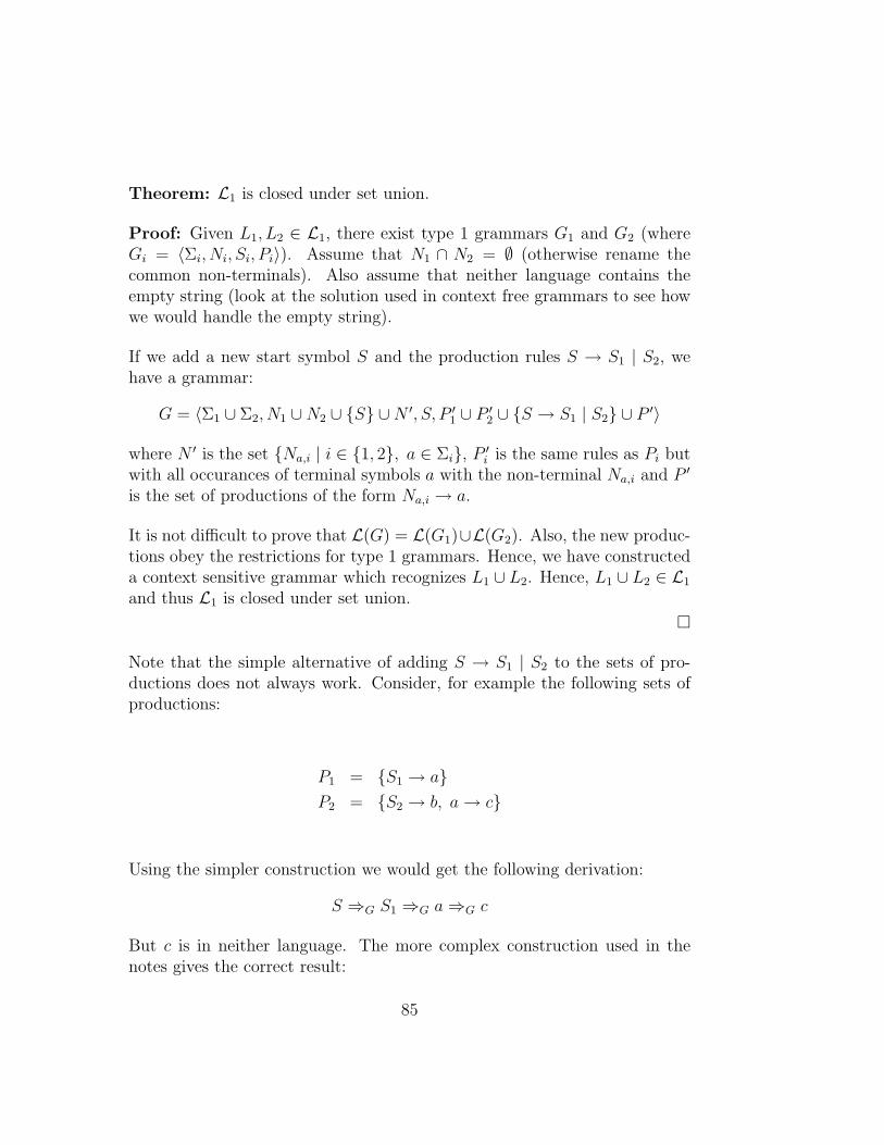
Theorem: L1 is closed under set union.

Proof: Given L1, L2 ∈ L1, there exist type 1 grammars G1 and G2 (whereGi = 〈Σi, Ni, Si, Pi〉). Assume that N1 ∩ N2 = ∅ (otherwise rename thecommon non-terminals). Also assume that neither language contains theempty string (look at the solution used in context free grammars to see howwe would handle the empty string).

If we add a new start symbol S and the production rules S → S1 | S2, wehave a grammar:

G = 〈Σ1 ∪ Σ2, N1 ∪N2 ∪ {S} ∪N ′, S, P ′1 ∪ P ′

2 ∪ {S → S1 | S2} ∪ P ′〉

where N ′ is the set {Na,i | i ∈ {1, 2}, a ∈ Σi}, P ′i is the same rules as Pi but

with all occurances of terminal symbols a with the non-terminal Na,i and P ′

is the set of productions of the form Na,i → a.

It is not difficult to prove that L(G) = L(G1)∪L(G2). Also, the new produc-tions obey the restrictions for type 1 grammars. Hence, we have constructeda context sensitive grammar which recognizes L1 ∪ L2. Hence, L1 ∪ L2 ∈ L1

and thus L1 is closed under set union.

�

Note that the simple alternative of adding S → S1 | S2 to the sets of pro-ductions does not always work. Consider, for example the following sets ofproductions:

P1 = {S1 → a}P2 = {S2 → b, a → c}

Using the simpler construction we would get the following derivation:

S ⇒G S1 ⇒G a ⇒G c

But c is in neither language. The more complex construction used in thenotes gives the correct result:

85

{ S → S1 | S2,S1 → Na,1,S2 → Nb,2,Na,2 → Nc,2,Na,1 → a,Na,2 → a,Nb,2 → b,Nc,2 → c }

What about catenation of languages? Initial attempts may not be veryfruitful. If we just add a new start symbol and a production S → S1S2 (whereS is the new start symbol and S1 and S2 are the old start symbols), adjacentsymbols derived from the different start symbols may react together. Forexample, consider language L which has a grammar with the the followingproductions:

{S → A | B, A → aA | a, B → b | bB, AB → c}

where S is the start symbol, clearly, none of the strings accepted by thisgrammar include c. But now consider if we add Sn → SS. This gives rise tothe following derivation:

Sn ⇒G SS ⇒G AS ⇒G AB ⇒G c

But c /∈ LL.

The next possible solution examined would be that of making an extra copy ofthe symbols (both terminal and non-terminal) where the symbols in the copyappear with a prime symbol (A′, a′) and are all non-terminal. Similarly, theproduction rules are copied renaming all occurrences of the symbols. Finallya new non-terminal symbol X is used as the start symbol, with the relatedproductions X → S1S

′2. Thus, no adjacent non-terminals can react together.

But we also have to add rules of the form a′ → a which can be performedprematurely and give problems due to reacting terminals, as is possible inthe following case:

{S → A | B, A → aA | a, B → b | bB, ab → c}

Again, c does not appear in any of the strings in this language, but the fol-lowing derivation is possible in the grammar derived by the above procedure:

86

X ⇒′G SS ′ ⇒′

G AS ′ ⇒′G AB′ ⇒′

G

aB′ ⇒′G ab′ ⇒′

G ab ⇒′G c

So, can it be done? The solution is to go one step further, as outlined in thefollowing theorem:

Theorem: L1 is closed under catenation.

Proof: Given L1, L2 ∈ L1, there exist type 1 grammars G1 and G2 (whereGi = 〈Σi, Ni, Si, Pi〉). Assume that N1 ∩ N2 = ∅ (otherwise rename thecommon non-terminals).

Define the prime operation on strings: a′ = a and (as)′ = a′s′. Extend thisoperation to work on productions (α → β)′ = α′ → β′ and on sets of stringsor productions: A′ = {x′ | x ∈ A}.

Now define a new grammar G = 〈Σ, N, S, P 〉, where:

Σdef= Σ1 ∪ Σ2

Ndef= N ′

1 ∪N ′′2 ∪ Σ′

1 ∪ Σ′′2 ∪ {S}

Pdef= P ′

1 ∪ P ′′2 ∪ {S → S ′

1S′′2} ∪ {a′ → a | a ∈ Σ′

1} ∪ {a′′ → a | a ∈ Σ′′2}

We can prove by induction that the language generated by this new (type 1)grammar is, in fact, L1L2.

Hence L1L2 is also of type 1.�

Theorem: L1 is closed under Kleene closure.

Proof: Let L ∈ L1. By definition, there exists a context sensitive grammarG = 〈Σ, N, P, S〉 such that L(G) = L.

The trick is to use the same solution as for catenation, and alternate betweenusing the primed symbols and the doubly primed symbols.

Define a new grammar with start symbol X (a new symbol), terminal symbolsΣ and non-terminal symbols the set: N ′ ∪ Σ′ ∪ N ′′ ∪ Σ′′ ∪ {X}. The set ofproduction rules allow us to produce arbitrary repetitions of alternating (old)

87

start symbols S ′ and S ′′: X → S ′ | S ′S ′′ | S ′S ′′X. We need to derive stringsin every occurrences and thus also add P ′ ∪ P ′′. Note that up to this pointwe can derive strings of the form x′1y

′′1x

′2y

′′2 . . . x′ny

′′n or x′1y

′′1x

′2y

′′2 . . . x′n where

each xi and yi is in L. Finally, we would like to remove those extra primesymbols: {a′ → a | a ∈ Σ}.

We can prove by induction that the language generated by this new grammaris, in fact, L∗. Also note that the new grammar is also of type 1.

Hence L∗ is also of type 1.

�

7.1.2 Recognition

As we have already seen, Turing machines are far too powerful when com-pared to type 1 grammars. Even restricting Turing machines to terminatingones (which must return 0 if the string is not in the language) is still toopowerful. And yet, pushdown automata are too weak to describe certaincontext sensitive languages. Can we find a class of machines, compromisingbetween NPDA and Turing machines, to recognize exactly the class of type1 languages?

The way we do it is by limiting the power of Turing machines. For conve-nience we will use non-deterministic Turing machines. Such a Turing machineis said to accept a string x, if when given input x, there is at least one se-quence of computations in which it will eventually terminate successfully.Otherwise, we say that the Turing machine rejects the string. Recall thatthe computational power of these machines is the same as that of a normalTuring machine. So how do we limit its power? The solution is quite simple.We just limit the length of tape it is allowed to use. Non-deterministic lin-ear bounded automata are simply non-deterministic Turing machines whichreceive their input between two special symbols �, � and may only use thetape between these two symbols.

Definition: A non-deterministic linear bounded automaton (LBA) is a non-deterministic Turing machine, 〈K, Σ, T, P,�,�, q1, F 〉 which is given inputbetween two special symbols �, �, with the head starting off on �. Themachine is not allowed to go to the left of � or to the right of �. Neitheris it allowed to overwrite them:

88

(q′, a, δ) ∈ P (q,�) ⇒ a =�, δ 6= L

(q′, a, δ) ∈ P (q,�) ⇒ a =�, δ 6= R

Linear bounded automata are powerful enough to recognize any context sensi-tive language. Since the productions are non-contracting (they cannot reducethe length of the derived string), any intermediate string in the derivationcannot exceed the length of the string we are trying to derive — the input.

Theorem: For any context sensitive language, there exists a linear boundedautomaton which recognizes it.

L1 ⊆ {L | L is recognized by a LBA }Proof: Let L ∈ L1. Then there is a type 1 grammar G which recognizes L.Consider a LBA M which has, in its tape alphabet the terminal symbols ofG and also pairs of symbols (both terminal and non-terminal) in G. If ε ∈ L,we first perform a simple check on the input. If there is no input (��) wemake the LBA terminate successfully if ε ∈ L, otherwise leave the actionundefined, hence rejecting it. Otherwise . . .

Initially, the input is relegated to the first bank (first elements of the pairs)and the machine writes S at the beginning of the second bank. Then, forevery production rule in P , the machine searches through the tape and per-forms any of the possible replacements (including shifting of the string ifnecessary), repeating until the two banks become equal. If this happens, theLBA terminates successfully. If no production rules are possible it fails.

Because of the nature of the production rules of type 1 grammars, if α∗⇒G β,

it has to be the case that |β| ≥ |α|. Hence, if x ∈ L then S+⇒G x and all

the intermediate sentential forms are at most |x| symbols long. Hence, themachine will terminate successfully returning 1 and thus x ∈ T (M).

If x /∈ L, there is no derivation of x from S and thus, M will never terminatesuccessfully. Hence x /∈ T (M).

Hence we have constructed a LBA M such that T (M) = L.�

Theorem: For every LBA M , T (M) ∈ L1.

Proof: The proof is very similar to the proof that every Turing machinehas an equivalent phrase structure grammar. If we take exactly the same

89

approach, we have a slight problem. At the end of the simulation, when weclean up the string, we will need to remove the left and right symbols and themachine state from the string. But this reduces the length of the sententialform which is not possible in a type 1 grammar. To solve this problem, weinclude these symbols on the tape into one symbol.

Let M = 〈K, Σ, T, P,�,�, q1, F 〉.

We will now construct grammar G = 〈T, N, S, R〉. The set of non-terminalstates will consist of 2 new symbols S and A and the set of symbols madeup of:

N1 = {(a, X) | a ∈ T, X ∈ Σ}

N2 = {(a, qX) | (a, X) ∈ N1, q ∈ K}

These are just like the ones used in the previous proof, but we include thestate in the non-terminal if it happens to be on that symbol.

N3 = {(a,� X) | a ∈ T, X ∈ Σ}N4 = {(a, X �) | a ∈ T, X ∈ Σ}N5 = {(a, qXY ) | q ∈ K, (a, XY ) ∈ N2 ∪N3}N6 = {(a, XqY ) | q ∈ K, (a, XY ) ∈ N2 ∪N3}

To accommodate the left and right symbols in the same non-terminal.

Ndef= {S, A} ∪

6⋃i=1

Ni

As before, we will have three collections of productions, one dealing withthe initialization, one with the emulation, and one dealing with the garbagecollection.

• Initialization: Initially we want to be able to build any non-emptystring within the left and right symbols and with the head on the leftsymbol:

90

S → (a, q1 � a)A for all a ∈ Σ \ {�,�}S → (a, q1 � a �) for all a ∈ Σ \ {�,�}

A → (a, a)A for all a ∈ Σ \ {�,�}A → (a, a �) for all a ∈ Σ \ {�,�}

• Simulation of LBA: Simulation of the machine is now more complicateddue to the extra non-terminals.

For every program instruction (q′, a′, S) ∈ P (q, a), we have three cases.

1. If a =�, we add the productions:

{(b, q � c) → (b, q′a′c) | b, c ∈ Σ}2. If a =�, we add the productions:

{(b, cq �) → (b, cq′a′) | b, c ∈ Σ}3. If a is neither � nor �, we add the productions:

{(b, qa) → (b, q′a′) | b ∈ Σ}∪ {(b,� qa) → (b,� q′a′) | b ∈ Σ}∪ {(b, qa �) → (b,� q′a′ �) | b ∈ Σ}

Similarly, we construct production rules for left and right movement.

We must also allow the grammar to reach a terminal string once a finalstate is reached:

{(a, qb) → a | a ∈ T, b ∈ Σ, q ∈ F}∪ {(a, bqc) → a | a ∈ T, b, c ∈ Σ, q ∈ F}∪ {(a, qbc) → a | a ∈ T, b, c ∈ Σ, q ∈ F}

• Garbage collection: Finally, once at least one symbol becomes terminal,so do all the others:

91

{(a, X)b → ab | X ∈ Σ∗, a, b ∈ T}∪ {a(b, X) → ab | X ∈ Σ∗, a, b ∈ T}

Clearly, G is of type 1. Also, it is clear (although we do not prove) thatG can generate any string, if and only if it is accepted by M . Hence, alllanguages which can be accepted by a LBA, can be generated by a contextsensitive grammar.

�

Corollary: L1 = {L | ∃M ∈ LBA · T (M) = L}

7.2 General Phrase Structure Grammars

While examining the properties of recursively enumerable languages, weproved that the class LE is, in fact, equivalent to the class of type 0 lan-guages — languages which can be generated by some phrase structure gram-mar. Hence, all the properties of class LE, are also properties L0. Theproperties we have proved are:

• closed under intersection

• closed under union

• closed under catenation

• not closed under complementation

Furthermore, since LE is the class of languages accepted by a Turing ma-chine, Church’s thesis says that if we define a larger class of languages, wecannot construct a machine which accepts the extra languages (otherwisethe machine is more powerful than a Turing machine). Hence, our faithin phrase structure grammars used to describe any meaningful language iswell-founded.

One remaining closure question which we have not yet answered is whetherL0 is closed under Kleene closure. The proof follows just like the one for L1

given earlier in this chapter.

92

Theorem: L0 is closed under Kleene closure.

Proof: Precisely the same construction as used to prove closure of L1 underKleene closure is used.

�

This ends our discussion of type 0 languages here, since we have alreadyproved the properties we may need to use. As a closing note, it is inter-esting to note that Chomsky and Turing were working independently whenthey defined their grammar hierarchy and machines respectively. The equiv-alence of the most general concept of computation was not limited to justthese, however. Other work done by Church on the Lambda calculus, Poston production systems, Smullyan on formal systems and Kleene in recursivefunction theory at approximately the same time also led to the same con-clusion. In other words, despite the various formalizations of a computationone may use, the resulting system was always most as powerful as a Turingmachine.

As an aside, I would like to point out similar results in other fields also firstencountered this past century:

• Quantum physics

• Godel’s Incompleteness Theorem

• Chaotic systems

• Inherent unfairness of any voting system

Not surprisingly, the philosophers of science have been kept very busy thispast century and in most cases, a lot of work still needs to be done before theycatch up. The only other such ‘disappointing’ result (in the sense that theyare all negative results which show that the way we have been looking at theworld needs to be thoroughly revised, and there is no hope in removing someinherent undesirable properties) was the realization that there are numbers(such as the square root of 2) which cannot be written as a fraction. Butthis is straying too far away from the original content of the course, and Iwill thus end this aside comment here.

93

7.3 Conclusions

We close this section by constructing a table with the properties of the lan-guage classes we have analyzed.

Recognizing ClosureLanguage Class Automaton L ∪M L ∩M L LM L∗

Free languages TM√ √

×√ √

Recursive Terminating TM√ √ √ √ √

Context sensitive LBA√ √ √

Context free NPDA√ √ √

Regular DFSA√ √ √ √ √

7.4 Exercises

1. Where does the proof that for every LBA there is an equivalent con-text sensitive language, fail if we try to extend it to general Turingmachines?

2. Discuss how one can directly construct a Turing machine which ac-cepts the Kleene closure of a recursively enumerable language. Hint:Recall how we proved that LE is closed under catenation and how oneenumerates N× N.

94

Part IV

Algorithmic Complexity

95

Chapter 8

Algorithm Classification

In the previous chapters, we have encountered the concept of unsolvability.This provides a useful classification of problems — we thus have two classesof problems, solvable and unsolvable.

However, this classification is far too general. Consider the class of solvableproblems. Within this equivalence class, some of the problems are moreequal than others. Although some problems may lie in this class, it is notguaranteed that they are solvable in practice. Recall that a Turing machinehas unlimited storage space and unlimited time in which to run. However,we live in a universe of limited resources. An algorithm is as good as uselessif it need 10 times the current age of the universe to execute, or needs morestorage cells than there are basic particles in the universe. Still, if we wereto draw an arbitrary line dividing useful from non-useful algorithms basedon the physical size or length of time it requires, it would be a subjectivematter1.

There is also another problem. As computers get faster, we would have toadmit more and more algorithms as useful. This all goes to show that placinga fixed limit on resources is not a very elegant way of solving the problem ofclassifying further the class of solvable problems.

The solution is to analyze the inherent complexity of algorithms. You havealready encountered complexity in previous courses. You may remember

1One may classify algorithms taking longer than a century to execute, but this didn’tstop an alien race from building a computer which took 5 million years to execute its pro-gram to find the answer to life, the universe and everything in Douglas Adams’ Hitchhiker’sGuide To The Galaxy.

96

that whereas adding a new element to the head of a linked list takes only aconstant amount of time (irrespective of the size of the list), sorting the listneeds on the order of n log(n) time units (where n is the length of the list).So which problems of which complexity will be classified as inherently toocomplex?

Consider a problem with complexity of the order n, where n is the size of theproblem. By doubling computer speed, in the same period of time, we cansolve a problem of twice the previous size. What about a problem of size n2.By doubling the speed, we can solve problems of up to 1.4 times the originalsize. But how about a problem of size 2n? By doubling speed, we are onlyincreasing the maximum size of the problem solvable in fixed time by 1. Thisshows an inherent difference between problems solvable in polynomial timeto those solvable in exponential time: whereas by multiplying the speed ofthe underlying machine, the size of solvable polynomial problems increasesgeometrically, this only grows arithmetically for exponential problems.

There still is a question of what model of computing we are allowed to use.Consider the following problem:

Traveling Salesman (TS)

Instance: Given a set of n cities C, a partial cost function of traveling fromone city to another cost (such that cost(c1, c2) is defined if there is a directmeans of traveling from city c1 to city c2, and if defined is the cost of thetraveling) and an amount of money m.

Question: Is there a way of traveling through all the cities exactly once,returning back to the initial city, and in the process not spending more thanthe amount of money m?

Consider a non-deterministic Turing machine, which will simply fan-out try-ing all possible paths. Clearly, in at most n steps, each path will either suc-ceed or fail. Hence, we will get a result in at most n steps. Hence, it seemsthat this problem is one of polynomial complexity. But non-determinism, in-volves, if you recall, an oracle function which tells us which path (if any) willyield results, or a machine with the ability to replicate itself for any numberof times. This is not a very realistic means of computation. So what if we tryto solve the problem on a deterministic Turing machine? If we enlist all thepaths and try them one by one, in the worst case, we will need to examine allpossible paths. This goes beyond the realms of polynomial complexity. You

97

may try to find an algorithm to solve the problem on a deterministic time,but it is very improbable that you will manage to do so.

Hence, the rudimentaries of a hierarchy start to become apparent. We willdefine the class of problems solvable in polynomial time on a deterministicTuring machine to be P . The class of problems solvable in polynomial time ona non-deterministic Turing machine will be called NP (non-deterministicallypolynomial). Beyond this, lie the problems which need exponential time evenon a non-deterministic Turing machine. There exist further classifications ofthis last class, but it is beyond the scope of this short part of the course todeal with these divisions.

Note that a number of problems have been shown to require exponential timeon a deterministic Turing machine. We refer to such problems as intractablebecause of the difficulties we encounter as soon as we try to apply thesealgorithms to modest sized instance of the problem.

Before concluding this brief introduction, a couple of questions arise from theabove text. First of all, does there exist a solution of the traveling salesmanproblem which uses only polynomial time on a deterministic machine? Andsecondly, why do we include this material together with language hierarchiesin a single unit?

Let us start with the initial question. Before, we consider the travelingsalesman, consider the following problem:

Less than or equal to (LTE)

Instance: Given two numbers n1 and n2.

Question: Is n1 ≤ n2?

Consider the deterministic Turing machine which performs this operation.It will terminate and succeed if the answer to the question is positive, butterminate and fail otherwise. One such machine overwrites the numbers (oneat a time) with a new symbol. If, the second runs out before the first, failbut terminate successfully otherwise:

98

( , ,R)

( , ,L)

E

( , ,R)

(1,1,R)

(*,*,L)( , ,L)

(1,*,L)

(1,1,R)

(1,*,R)

(1,1,L)(1,1,L)

(*,*,R)

q1

First number has run out first

No transition if second numberruns out first

Each right-left trip will take about 2(n1 +2) steps. This will have to be donefor n1 times. Hence, the machine terminates after at most αn2

1 + βn1 + γsteps. Since the machine is a deterministic one, and it takes only a poly-nomial amount of time (relative to the size of the input), this problem isin P . Clearly, every deterministic Turing machine can be seen as a non-deterministic one and thus, it can also be solved by a nondeterministic Turingmachine in polynomial time and is hence also in NP.

How about the traveling salesman’s problem? We have already given a roughidea of how to construct a non-deterministic Turing machine which computesthe answer in polynomial time. Hence it is in NP. But is it also in P? This isprobably one of the most sought after answers in mathematics today. Nobodyhas come up with an algorithm showing that it is in P , but, on the otherhand, nobody has come up with a proof that this is impossible. The mysteryis even more intriguing than this. There is no problem known to be in NPbut not P .

In 1971, an important paper identified a problem, the satisfiability problem,and showed that it is the hardest problem in NP. Hence, if it is shown to bein P , so must all the other problems in NP, and P =NP. Further work donein these past 30 years has identified a number of other such hardest problemsin NP. Amongst these is the traveling salesman problem.

The general consensus, is that NP 6= P and hence the traveling salesmanproblem is intractable and not in P , but this still has to be proved.

As for the inclusion of this material together with language hierarchies, wenote that we are basically using the Turing machines as language recognizers.We have a decision problem Π which, divides the set of possible inputs intotwo: the instances answered positively and those answered negatively, whichare complements of each other. Hence, our questions are all dealing with thecomplexity of the language in question. Note that we are only dealing with

99

recursive languages, since we assume that the Turing machine terminateswith a yes or no answer. This provides us with yet another hierarchy oflanguages. Unfortunately, due to lack of time, we will not be able to comparethis hierarchy with the Chomsky one.

8.1 Exercises

1. Show that the following problem is in P :

Triangle (TRI)

Instance: Given three numbers.

Question: Can these three numbers be the lengths of the three sidesof a triangle?

2. Show that the traveling salesman’s problem but with distinct start andterminal cities is also in NP. We have, in passing, mentioned that thetraveling salesman problem is the hardest problem in NP . In effect, ifwe show that the traveling salesman is in P , then so are all the othermembers of NP . Can you outline, how to show that the modifiedproblem given here is also, in the same sense, the hardest NP problem?

100

Chapter 9

Definitions and Basic Results

9.1 Background

We will now start formally defining what we mean by the complexity of aproblem. We will only be treating problems with a yes/no answer and forwhich there exists a terminating algorithm which gives the answer. Thefollowing definitions regarding complexity are based on languages. This mayseem strange, but the concept of a yes/no decision problem is intimatelyrelated to languages.

Consider a problem Π. There is the set DΠ of strings which the problemaccepts as input. Of these, the strings in the set YΠ are those which give apositive answer whereas NΠ are those which give a negative answer. Clearlya Turing Machine which computes the answer to this problem is basicallydeciding whether the given input string in DΠ is in the language YΠ. Hence,if we define the complexity of deciding whether a string lies in a particularlanguage or not we can apply these results to decision problems in general.

The format in which we will present decision problems is as follows:

Primality test (PRT)

Instance: Given a number n.

Question: Is n a prime number?

The first line states the name of a decision problem (in this case, primalitytest) and a short version of the name which will be used as an abbreviation(PRT). We then specify what an instance of the problem consists of. In this

101

case it is a number n. This can be seen as the formal parametrisation ofthe input of the problem. Finally, we ask a yes/no question regarding theinstance.

Our main task is to decide how much work has to go into showing that aparticular instantiation of the input is in the language of positive answersor not. Obviously, certain inputs inherently require more work than others.For example, consider the problem of checking whether a given word is ina given dictionary. The problem becomes more ‘complex’ as the size of thedictionary increases. The complexity of the problem is thus to be given asa function of the size of the dictionary. This is not very convenient, sincefor every decision problem we must first isolate the inputs on which theproblem complexity depends. However, there is a simpler solution whichwe will adopt. Given a reasonable encoding of the inputs, we will calculatethe complexity of the problem as a function which, given the length of aninput, gives the complexity of calculating the result. Consider the dictionaryproblem once more. We are now giving the complexity of computing theresult in terms of, not just the dictionary size, but also the size of the wordwe are searching for. This makes sense, since every time we check whethera particular dictionary entry matches the searched word, we need to lookthrough the symbols of the word to check for equality, and hence, the longerthe word, the more work needs to be done.

Now consider the complexity of a particular algorithm to solve the dictionaryproblem. As you should already be aware, there is a variety of complexity(execution length) measures we can take. The ones we are usually interestedin are the average and worst case length of execution. In this course we willbe interested exclusively in the worst case analysis.

To classify a problem we use the big-O notation. Since it is difficult tocalculate the exact number of execution steps of an algorithm (and it isdependent on the amount of effort put into making it more efficient), thebig-O notation allows us to approximate an upperbound to a function. Theformal definition is the following:

Definition: We say that a function f(n) (f : N → R+) is O(g(n)), some-times written as f(n) = O(g(n)) if there is a constant c, such that, beyonda particular value of n, c g(n) ≥ f(n):

∃c : R+, n0 : N · ∀n : N · (n ≥ n0 ⇒ c g(n) ≥ f(n))

102

For example, you may recall that 7n2 + n− 4 is O(n2), since for non-zero n(n0 = 0), 8n2 ≥ 7n2 + n− 4 (c = 8).

Similarly, 2n + n100 is O(2n), since for any n ≥ 1000, 2 · 2n ≥ 2n + n100.

Finally, there is still an ambiguity in the description we have given. We havestated that the input is reasonably encoded. What exactly do we mean bythis?

Some encodings are obviously unreasonable. Consider a Turing machinewhich checks whether two given strings are equal. There is a simple algorithmwhich goes back and forth to check the symbols for equality. Assume thatthe first string is m symbols long. Clearly, it needs, at most, m + 1 runs tocheck each of the m symbols, and in each run it moves the head m+1 spacesto the left and then m symbols to the right. Hence, we have a machine takingabout m(m+1+m). Since the total length of the input n ≥ m symbols long,the execution length is not larger than n(2n + 1), which is O(n2). But now

consider the encoding of the input w1 and w2 as (w1�w2�)|w1w2|. Usingprecisely the same algorithm but ignoring the extra symbols which we willnot use, the analysis now yields a worst case taking O(n). This is becausewe are using an unreasonable encoding.

Reverting back to Turing machines as language acceptors bypasses the prob-lem very neatly. It is now clear that the two machines are accepting consid-erably different languages. The first machine accepted exactly those stringsin {w�w | w ∈ Σ∗} and rejected all those in {w�w′ | w, w′ ∈ Σ∗, w 6= w′}.On the other hand, the second machine is accepting strings in:

{(w�w�)2|w| | w ∈ Σ∗}

but rejected strings of the form:

{(w�w′�)|ww′| | w, w′ ∈ Σ∗, w 6= w′}

Note that we assume that the input lies in the domain of the language.

But we eventually want to apply this knowledge to actual problems. There isno hard and fast way of defining what a reasonable encoding is. It is usuallyused to denote a mixture of conciseness (without unnecessary padding as wasused in the example) and decodability (the ability to decode the the inputinto a usable format using an algorithm of O(nα), where α is a constant).

103

9.2 Machine Complexity

Until now, we have only looked at Turing machines as a means of productionof an output. We have not analyzed the length of such executions. Thisis what we set out to do in this section. The basic machine we will belooking at is a single (two-way) infinite tape machine. Furthermore, wewill be looking at terminating Turing machines used to give a yes/no answerdepending whether they terminated successfully or not (hence we are ignoringthe output).

Definition: A terminating deterministic Turing machine is said to havecomplexity t (where t is a function from natural numbers to natural numbers)if, when given input x, the length of the derivation is not more than t(|x|).

Note that we are looking at the worst case. Consider the list of all sin-gle character inputs x1, x2, . . .xn. Assume that they respectively take l1,l2,. . . ln transitions to terminate. Then, the definition states that t(1) ≥max{l1, l2, . . . ln}.

Here, we are talking about single tape Turing machines. Usually it is muchmore convenient to be able to use, at least, multiple tape machines in ourconstructions. However, the extra tapes may allow us to perform certainproblems faster than on a single tape machines, and our results for the con-struction we give would not be comparable to the real complexity as definedabove. To get around this problem, we prove a theorem which relates thecomplexity of a k-tape Turing machine with that of a single tape machine.

Theorem: Provided that t(n) ≥ n, a k-tape Turing machine of complex-ity t(x) can be simulated on a single tape Turing machine with complexityO(t2(x)).

Proof: We give the construction of a single tape Turing machine which cansimulate a multi-tape Turing machine, and then we analyze the complexityof the resultant machine.

The emulator will separate the contents of the k tapes by a special symbol? and will have extra symbols, such that the contents of the location of theheads will be marked by the symbol with a bar over it. Hence, the tapecontents ?abaa ? � ? a? represents a 3 tape machine, where the first tape hasthe contents abaa and the head lies on the b, the second is still unused andthe third contains a single symbol over which the head resides.

104

The emulator, upon input w = av, will follow this program:

1. Write on the tape the initial configuration: ?av ? (�?)k−1.

2. To simulate a single move, the machine scans the input from the first? to the (k +1)th to note what is under the heads. Then a second passis made to update the tapes accordingly.

3. If, at any point the machine tries to move a virtual head onto a ?, it willreplace the position by a blank and shift the symbols in the requireddirection.

Clearly, the initial stage takes O(n) steps. The second and third stage re-quires two scans and up to k shifts. Each scan and shift requires a numberof steps of the order of the length of the strings stored on the tape. Clearly,these cannot be any longer than the length of the complete execution of the k-tape machine. Hence, every time the second and third stages are performed,they take O(t(n)). However, these will be performed up to t(n) times, andhence the total complexity is:

O(n) + t(n)O(t(n))

Since we assumed that t(n) ≥ n, this reduces to O(t2(n)).�

We could do the same with other extensions of Turing machines, but k-tape Turing machines are generally sufficient to allow clear descriptions ofalgorithms. However, in certain problems, such as the traveling salesmanproblem as defined in the previous chapter, we will be better off using non-deterministic Turing machines. The importance of these machines will berealized later, as we discuss such algorithms into more detail. For now,we will just give a definition of what we mean by the complexity of a non-deterministic Turing machine (the complexity of a multi-tape Turing machinefollowed naturally from that of a single tape machine, which is why we didnot give it).

Definition: A terminating non-deterministic Turing machine is said to havecomplexity t (where t is a function from natural numbers to natural numbers)if, when given input x, the length of the longest branch of execution (whetherit terminates successfully or not) is t(|x|).

105

Since deterministic Turing machines are all-powerful, they can also simu-late non-deterministic Turing machines. This is obviously done at a price.The following theorem relates the complexity of a non-deterministic Turingmachine with that of a deterministic one emulating it.

Theorem: Provided that t(n) ≥ n, a non-deterministic single tape Turingmachine of complexity t(n) can be simulated on a single tape deterministicTuring machine with complexity 2O(t(n)).

Proof: As before, we construct an emulator and then analyze its complex-ity. To emulate a non-deterministic Turing machine, we use a 4-tape Turingmachine. The deterministic machine proceeds to enumerate all possible com-putations and executes then in sequence. The four tapes are used as follows:

1. The first tape stores the input string which it does not modify in anyway.

2. The second tape is used as a working tape when emulating a particularinstance of the non-deterministic machine.

3. The third tape is used to store the possible computations which wehave already tried.

4. The last tape is used to hold a flag to remember whether there was acomputation of the length currently being investigated which has notterminated.

The main problem is that of enumerating all possible computation paths.Consider the largest size of the sets in the range of P . This corresponds to themaximum number of possibilities we have at any point in the computation.Let this number be α. Clearly, if we enumerate the contents of the sets inthe range of P , we can describe any computation with input w as a sequenceof numbers in 1, 2, . . . α. At every stage, if P (q, a) is the set of possibilitiesfrom p1 to pm, the next number i in the list will determine which pi to follow.Obviously, not all strings over this alphabet are valid computations.

In particular, note that if a string is rejected, there is a maximum length be-yond which all computation sequence strings over {1, . . . α} will either rejectthe input (not necessarily using up all the computation sequence string), orgive an invalid computation (in that a choice of a non-existent path is made).This number is the maximum depth at which the rejection occurs.

106

Now consider the following algorithm:

1. Copy the contents of tape 1 to tape 2.

2. Simulate the non-deterministic machine using the string on tape 3 totake decisions as to which path to follow. A number of possibilities canoccur:

If a decision is to be made about which path to follow but no moresymbols remain on tape 3 jump to step 3.

If an invalid computation occurs (the next symbol on tape 3 is largerthan the set of next possibilities) or a rejecting configuration is encoun-tered jump to step 4.

If, however, an accepting configuration is encountered, accept the inputand terminate.

3. Write a symbol ? on tape 4.

4. Calculate the next string over {1, . . . α} to be written on tape 3. Theseare to be produced in order of the length of the string (and alphabeti-cally for strings of the same length).

If it is longer than the previous string then check tape 4. If there is ablank symbol (no ? written on the tape), then all the paths were eitherinvalid, or produced rejecting computations. Terminate and reject. Ifthere is a ?, then there must have been some, as yet unterminatedcomputations and we need to check computations of a longer length.Clear tape 4.

Jump to instruction 1.

It should be clear (although not necessarily easily provable) that this emu-lator terminates and accepts exactly when the original machine did so, andterminates and rejects when the non-deterministic machine did so.

For an input of length n, the maximum depth of the computation tree ist(n). At every stage, there are at most α siblings of a particular node.The total number of nodes, thus cannot exceed αt(n) and is thus O(αt(n)).The time taken to travel down the tree path to a node does not take more

107

than O(t(n)) steps. Hence, the running time of the resultant machine isO(t(n))O(αt(n)). This is 2O(t(n)). But the machine we used had 4 tapes. Bythe previous lemma, this can be simulated on a single tape machine withcomplexity (2O(t(n)))2 = 2O(2t(n)) = 2O(t(n)).

�

Note that this theorem does not say that it is impossible for a deterministicTuring machine to emulate a non-deterministic one in less than exponen-tial time, but that we know of an algorithm which needs this amount oftime. Hence, we have established an upperbound for the complexity of thissimulation.

9.3 Complexity Classes

9.3.1 Class P

Clearly, we can classify languages by the complexity of a Turing machineneeded to decide the language. As already indicated before, we will classifytogether all languages which need a polynomial complexity single tape de-terministic Turing machine to decide them. This is the class of languagesP .

Definition: P is the class of languages decidable in polynomial time on adeterministic single tape Turing machine:

Pdef= {L | L decidable by deterministic T such that

complexity of T is O(nk) for some k ∈ N }

At this point it is worth reviewing the definition of what it means for a lan-guage L to be decidable by Turing machine M . It means that M terminateson all inputs, successfully if the input is in L, but failing if it is not. It isclear, thus, that we are restricting our analysis to recursive languages.

We have already shown, for example, that checking whether a given word isin a given dictionary is a problem in P . We will give another example beforegoing on to further classes.

Example: Consider the following problem:

108

Directed path (PATH)

Instance: Given a directed graph G and two nodes n1 and n2.

Question: Is there a path from n1 to n2?

We will show that PATH ∈ P , by constructing a polynomial time algorithmworking on a deterministic Turing machine which solves the problem.

1. Mark node n1.

2. For every edge (a, b) such that a is marked, mark also b.

3. If some new nodes have been marked, go back to 2.

4. Accept if n2 is marked, reject otherwise.

The first and last steps are executed just once (and take only, at most O(n)steps to locate n1 and n2). Step 2 scans every edge, checks the first nodeand may mark the second. This can be easily done in polynomial timeon a deterministic machine (scanning every edge takes O(n) and in everycase checking the first node and possibly marking the second will only takeO(n), hence taking O(n2)). Finally step 2 is repeated for a number of times.Consider the count of marked nodes which starts at 1 and increases everytime step 2 is executed. Clearly, this cannot go on more than the number ofnodes we have. Hence, the maximum number of repetitions is O(n). Hence,the total complexity is:

O(n) + O(n2)O(n) + O(n) = O(n3)

Hence, PATH ∈ P .�

Theorem: The class of languages recognizable by k-tape Turing machinesin polynomial time is P .

Proof: Let M be a k-tape Turing machine such that it is decidable in O(nα)(α ∈ N) steps. By the theorem relating multi-tape Turing machines withsingle tape ones, we have that it is decidable in O(n2α) on a single tapemachine. Hence, it is in P . Note that in the case of α = 0, if f(n) = O(1)then f(n) = O(n). Hence we can still apply the emulation theorem.

Conversely, if L ∈ P then there is a single tape deterministic Turing machinewhich decides L. But we can run M on a multi-tape machine which ignores

109

all but the first tape. This emulation takes exactly as many steps as theoriginal machine. Hence, L is decidable in polynomial time on a k-tapemachine.

�

9.3.2 Class NP

The theorem which constructed a non-deterministic Turing machine emulatorrunning on a deterministic Turing machine, stated that we can perform thisemulation approximately in the exponent of the original time taken by a non-deterministic machine. It does not state that there is not a more efficientemulation. However, if there is one, we do not yet know about it. This meansthat the class of languages decidable on a non-deterministic Turing machinein polynomial time is not necessarily the same as P . With this in mind, wedefine the class NP:

Definition: NP is the class of languages decidable in polynomial time on anon-deterministic single tape Turing machine:

NPdef= {L | L decidable by non-deterministic T such that

complexity of T is O(nk) for some k ∈ N }

NP stands for non-deterministically polynomial.

The first thing we note is that class P is contained in class NP:

Theorem: P ⊆ NP

Proof: The proof is trivial. Every deterministic Turing machine can be seenas a non-deterministic Turing machine with no choices. Hence, the time com-plexity of a deterministic Turing machine is the same as when interpretedas a non-deterministic Turing machine. Thus, all polynomial time determin-istic machines run in polynomial time on a non-deterministic machine andtherefore P ⊆ NP.

�

Example: Let us look at a problem encountered on a multiprocessor system:

Scheduler (SCH)

110

Instance: Given a set T of tasks, a time cost function c associating apositive cost with every task, a number of processors p and a deadline D

Question: Can the tasks be scheduled in the given deadline? Or moreprecisely, is there a partition of T , T1 . . .Tn such that:

D ≥ max{∑

t∈Tic(t) | 1 ≤ i ≤ n}

We prove that SCH ∈ NP. Consider the non-deterministic Turing machinewhich goes through all the tasks assigning each one to a processor non-deterministically. At the end, the total time taken is calculated and checkedagainst D. If it larger than D, the machine terminates and fails, otherwise itterminates and succeeds. Clearly, the algorithm always terminates. If there isany assignment which will work it will be tried and the machine will succeedand accept the input, but if there are none, the machine fails and rejectsthe input. The assignment of tasks to processors takes O(n) steps. Addingtwo numbers can be done in polynomial time and thus so can the adding ofO(n) numbers. Finding the maximum of a set of p elements is also O(n) as iscomparison of numbers. Hence, the total time taken by any path is O(nα) forsome particular value of α. Hence, we have constructed a polynomial timenon-deterministic Turing machine which decides SCH. Hence SCH ∈ NP.

�

There is a particular property you may have noticed, which this problemenjoys. If we find a solution, it is very easy to show that it is, in factcorrect. As we have already said, we can calculate whether a given assignmentof tasks to processors satisfies the deadline constraint in polynomial timeon a deterministic machine. Even in the traveling salesman case, we cancount the values on the claimed paths and compare the result to the upperbound in polynomial time on a deterministic machine. This is the conceptof polynomial verifiability. Basically, a problem is polynomial verifiable if,given an answer, we can easily verify its correctness. This can be formalizedinto:

Definition: An algorithm M is said to be a verifier of a language L whenw ∈ L if and only if there exists a string c, such that M accepts (w, c).

c is sometimes called a certificate, and it is left out in the analysis of thecomplexity of M .

The idea is that M accepts strings if and only if they are followed by aninstance proving their membership in L. In the case of the traveling salesman,

111

a verifier V would be an algorithm which, for every instance of the problem,V accepts the instance exactly when we can add extra information to theinput.

A Turing machine solving the problem from scratch is a special case of averifier where c = ε in all cases. However, we started discussing verifiersbecause we know that the solution we gave for the traveling salesman problemis not very efficient, even though we know that we can verify an answerquickly. This can be generalized into a surprising result:

Theorem: A language L is in NP if and only if it has a verifier in P .

Proof: Assume L ∈ NP. We need to show that it has a polynomial timeverifier (in P ). Consider the following algorithm V working on input (w, c):

1. Simulate the non-deterministic machine with input w and using c asthe non-deterministic path to take (as in the deterministic emulationof non-deterministic machines).

2. If this path of the computation accepts, accept the input. Otherwise,reject.

Clearly, there is a string c such that (w, c) is accepted if and only if w ∈ L.Also, the machine runs in polynomial time. Hence L has a verifier in P .

Conversely, let L have a verifier in P , namely V . Assume that V has timecomplexity nα. Now consider the following non-deterministic machine M ,working on input w:

1. Branch (non-deterministically) to all strings c of length nα.

2. Run V on (w, c).

3. If V accepts, accept, otherwise reject.

Obviously, V can never look at strings longer than nα. Hence, if w ∈ L thenthere is a string c such that |c| ≤ nα such that V accepts (w, c). Clearly sucha path would exist on M and thus the string would be accepted. On theother hand, if w /∈ L, there is no c such that V accepts (w, c). Thus there isno path in M accepting w, and hence it is rejected.

Also, since V has polynomial time, so has M , and thus L ∈ NP.

112

�

Thus, whenever we want to show that a given decision problem is in NP wenow have two approaches we can take. We can either stick to the definitionand show that there is a non-deterministic machine which computes theanswer in polynomial time, or we may show that it is easy to check whethera given answer is correct or not. In most cases, both approaches are quiteeasy to use. The result is more important from a conceptual point of view.The class NP can be characterized in two alternative ways, neither of whichclearly indicates whether there are problems in NP which are not in P . Thisis the question we will be tackling for the rest of this course, but for which,unfortunately, will not be able to furnish an answer.

9.4 Reducibility

A psychologist analyzing the mathematical mind asked the following questionto a mathematician:

You are walking down a street where you see a burning house, a fire hydrant,a box of matches and a hosepipe. What do you do?

After careful thought, the mathematician answered:

I simply connect the pipe to the hydrant, turn on the water and extinguishthe fire.

Satisfied by the answer, the psychologist asked another question:

You are now walking down a street where you see a house, a fire hydrant, abox of matches and a hosepipe. What do you do?

Without even pausing for thought, the mathematician answered:

I light a match, set the house alight, and it has now been reduced to a previ-ously solved problem.

In mathematics, the concept of reducing a problem into a special case of analready known one is a very important technique. The area of algorithmcomplexity is no exception and in this section we will define what it meansfor a problem to be reducible to another and how this technique can be usedeffectively.

Consider the following problem:

113

Transitive acquaintance (TA)

Instance: Given set of people, a list of who knows whom and two particularpersons p1 and p2.

Question: Is p1 a transitive acquaintance of p2?

We say that p1 is a transitive acquaintance of p2 if, either p1 is a acquaintanceof p2 or there is an intermediate person p such that p1 is a acquaintance of pand p is a transitive acquaintance of p2. Is this problem in P?

With a little bit of insight we realize that this problem is simply a rewordingof the PATH problem. If we label the nodes by people’s names, and maketwo edges (a, b) and (b, a) for every pair of people a and b who know eachother (assume that acquaintance is mutual), we can run the PATH algorithmand solve the problem in polynomial time.

Since we can build the graph in polynomial time, and PATH ∈ P , we imme-diately know that MA∈ P . How can we formalize this concept of a problembeing reducible to another?

Definition: A language L1 is said to be polynomially reducible to anotherlanguage L2, written as L1 �P L2, if there is a total function f : L1 → L2

which is computable in polynomial time on a deterministic Turing machine,such that

w ∈ L1 ⇔ f(w) ∈ L2

To show that TA �P PATH we need to define function f , which given aninstance of TA gives an instance of PATH. This function, is the one alreadydefined: f(〈P, A〉) = 〈P, A ∪ A−1〉 (where 〈P, A〉 is an instance of the ac-quaintance problem — P is the set of people and A the set of acquaintances,and 〈N, E〉 is an instance of PATH if N is the set of nodes and E the set ofedges). This function can clearly be calculated in polynomial time since itrequires only copying.

Since PATH ∈ P and TA �P PATH we expect to be able to conclude thatTA ∈ P . This is proved in the following theorem:

Theorem: If L1 �P L2 and L2 ∈ P then L1 ∈ P .

Proof: Simply compute function f , taking O(nα) steps, then execute thealgorithm deciding L2, taking O(nβ). Now w ∈ L1 if and only if f(w) ∈L2. Hence this algorithm decides L1. Its complexity is O(nα) + (nβ) =O(nmax(α,β)) and L1 is hence in P .

114

�

Note that the function need not be as simple as the one for TA. Consider thefollowing extension of the problem:

Country acquaintance (CA)

Instance: Given set of people and their nationality, a list of who knowswhom and two distinct countries c1 and c2.

Question: Is there a person from c1 who is a transitive acquaintance of aperson from c2?

We will show that CA�PTA, by giving a function which maps any instanceof CA into an instance of TA.

We start by building a graph as we did in TA. Now we add a person p1 suchthat p1 knows all people from c1 and nobody else. Similarly, we add p2 forc2. Clearly, this means O(n) more edges. We now ask the TR question onp1 and p2. This function is computable in polynomial time. Now, if someperson q1 in c1 transitively knows some person q2 in c2, then p1 knows q1

who transitively knows q2 who knows p2. Hence p1 knows p2. Conversely,if p1 knows p2, then p1 knows somebody q1 (who must be from c1) whotransitively knows p2. But p2 knows only people of c2 (which is differentfrom c1) and hence there must be a person q2 from c2 who knows p2 and suchthat q1 transitively knows q2. Hence there exist q1 from c1 and q2 from c2 whoare transitive acquaintances. Hence, w ∈ CA ⇔ f(w) ∈ TA and thereforeCA �P TA. But TA ∈ P and hence CA ∈ P .

Before we conclude this section we give a few properties of the reduciblerelation.

Proposition: The reducible relation (�P ) is reflexive and transitive. AlsoP × NP ⊆ �P .

9.5 NP-completeness

The main use of reducibility, is however not in P , but in NP. The followingtheorem can easily be proved:

Theorem: If L1 �P L2 and L2 ∈ NP then L1 ∈ NP.

Reducibility is basically a measure of how hard a problem is. When wesay that L1 �P L2, we are basically saying that (ignoring any ‘insignificant’

115

polynomial delays) deciding L2 is at least as hard as deciding L1. Is there aproblem which is the hardest in NP?

Assume there is, and let us call the problem X. Thus, for any languageL ∈ NP, L �P X. Now assume that somebody manages to show thatX ∈ P . By the theorem we have proved earlier, L �P X and X ∈ P impliesthat L ∈ P . Hence, the whole of NP would collapse to P . Therefore, if sucha problem exists, researchers can concentrate exclusively on whether X ∈ P .There turns out to be not just one, but a whole family of such problems. Wecall this family of functions NP-complete and it is defined as follows:

Definition: A language L is said to be NP-complete if:

• L ∈ NP

• For every language L′ ∈ NP, L′ �P L.

The property that if we find an NP-complete problem to lie in P then thewhole of NP would collapse to P , can now be proved.

Theorem: If NP-complete ∩ P 6= ∅ then P = NP.

Proof: Recall that if A �P B and B ∈ P then A ∈ P .

Assume NP-complete ∩ P 6= ∅ and let X be one element from this set.Consider any Y ∈ NP. By the definition of NP-completeness, Y �P X. ButX ∈ P . Hence Y ∈ P . Therefore NP ⊆ P . We also proved that P ⊆ NPand therefore P = NP.

�

Assume we know at least one NP-complete problem X. If we find an NPhard problem Y such that X is reducible to Y , then Y is at least as hard asX and Y should therefore also classify as ‘the hardest problem in NP’. Thefollowing theorem proves this result.

Theorem: If L is NP-complete and L �P L′ (where L′ ∈ NP) then L′ isalso NP-complete.

Proof: To prove that L′ is NP-complete, we need to prove two properties:that it is in NP and that all NP hard problems are reducible to L′. The firstis given in the hypothesis. Now consider any NP hard problem X. Since Lis NP-complete, we know that X �P L. But we also know that L �P L′.Hence, by transitivity of �P , we get X �P L′.

116

�

We will now end this chapter by the grand proof of this part of the course.Originally given in a pioneering paper by Cook in 1971, this theorem givesus a first NP-complete problem which we can then use to prove that otherproblems are NP-complete.

9.6 Cook’s Theorem

Before we state the theorem and proof, we need some background informationabout Boolean logic, which is the domain of the problem given in Cook’stheorem.

Given a set of Boolean variables V , we call a total function s : V → {T, F}a truth assignment. We say that variable v is true under s if s(v) = T .Otherwise we say that v is false under s.

Literals can be either a variable, or a variable with a bar over it v (corre-sponding to not v). We can extend s to give the truth value of literals in thefollowing manner: given a variable v, s(v) = T if s(v) = F , otherwise it isequal to F .

A set of literals is called a clause (corresponding to disjunction). The inter-pretation of s can be extended once more to get:

s(C) =

{T if ∃c ∈ C · s(c) = TF otherwise

Finally, a set of clauses is said to be satisfiable under interpretation s if forevery clause c, s(c) = T .

We can now state Cook’s theorem.

Theorem: SAT ∈ NP-complete, where SAT is defined as:

Satisfiability (SAT)

Instance: Given a set of variables V and a set of clauses C.

Question: Is there a truth assignment s satisfying C?

Comment: If you recall Boolean logic, a collection of clauses is effectivelyan expression in disjunctive normal form. Also, all boolean expressions are

117

expressible in disjunctive normal form. Hence, we are effectively showingthat checking whether a general boolean expression can be satisfied is NP-complete.

Proof: That SAT ∈ NP is not hard to prove. Consider the problem ofdeciding whether a given interpretation satisfies C. For every variable v ∈V we pass over C to replace literals v and v by T or F . Another passover C replaces clauses by T or F . Finally a last pass is needed to checkwhether each clause has been satisfied or not. Clearly, this takes polynomialtime. Effectively, we have constructed a polynomial verifier for SAT . Thisguarantees that SAT ∈ NP. (alternatively we could have gone on to constructa non-deterministic Turing machine which tries all possible truth assignmentsat once.

We now need to prove that all problems in NP can be reduced to SAT. Con-sider L ∈ NP. We need to prove that L �P SAT. What do we know about L?The property defining NP guarantees that there is non-deterministic Turingmachine which decides L in polynomial time. What we thus try to do, istransform a non-deterministic Turing machine into an instance of SAT. Ifthis can be done in polynomial time, we can transform L into an instance ofSAT via the non-deterministic Turing machine which recognizes L, whateverL might be.

Let M be a terminating non-deterministic Turing machine such that M =〈K, Σ, T, q1, P, F 〉. We now set up a set of Boolean clauses such that theycan be satisfiable if and only if an input string is accepted by M . We thenshow that this construction is possible in polynomial time.

What boolean variables do we need? We need to remember the followinginformation:

• In what state is M at time t? If we enumerate the states starting fromq1 up to q|K|, we can have variables tQi which is true if and only if M

is in state qi at time step t.

• Which tape square is the head scanning at time t? We will use tHi

which is set to true if and only if the head is scanning square i at timet.

• What are the contents of the tape? If we enumerate the tape symbolsas σ1 to σ|Σ|, we can use variables tS[i]j which is true if and only if

square i has symbol j at time t.

118

But we have to place bounds on the subscripts of the above variables. Recallthat M has polynomial complexity p(n). In this time it cannot use anytape square not in S[−p(n)] . . .S[p(n)]. Similarly, the time variables cannotexceed p(n). The result is that each subscript has O(p(n)) possible values.Hence, we have O(p2(n)) + O(p2(n)) + O(p3(n)) variables which is O(p3(n))— a polynomial in n.

Now, we will give a set of clauses C which can be satisfied if and only if Maccepts the input in at most p(n) steps. Hence:

w ∈ L

⇔ M accepts x

⇔ M accepts x in at most p(n) steps

⇔ C can be satisfied

We now set out to define the clauses. We will have four sets of clauses. Eachwill serve a specific function:

1. Machine invariants, split into three subclasses:

(a) M can only be in one state at a time.

(b) The head can only be at one position at a time.

(c) Each square can only contain one piece of information at a time.

2. Initialization of the machine.

3. Application of P to calculate the next state, position and tape contents.

4. Termination of the machine.

We now define the clauses.

1. Machine invariants:

(a) One state at a time: The machine has to be in at least one stateat any time t. For t ranging over: 0 ≤ t ≤ p(n) . . .

{tQ1, tQ2 . . .t Q|K|}

119

But there may be no more than one state which is true. This isexpressible as ¬(tQi ∧t Qj) where i 6= j. In disjunctive form, thisappears as:

{tQi, tQj}

where 0 ≤ t ≤ p(n) and 1 ≤ i < j ≤ |K|.

Note that we O(|K|2) of these clauses. Hence, the encoding of theclauses of this type is polynomial in size.

(b) The head is at one place at a time: This is almost identical to theprevious case:

{tH−p(n), . . .t Hp(n)}

where 0 ≤ t ≤ p(n) and . . .

{tHi, tHj}

where 0 ≤ t ≤ p(n) and −p(n) ≤ i < j ≤ p(n).

As before, the encoding of these clauses only takes O(p2(n)), whichis a polynomial.

(c) Tape squares can contain only one piece of information at a time:

{tQ[s]−p(n), . . .t Q[s]p(n)}

where 0 ≤ t ≤ p(n) and 1 ≤ s ≤ |Σ| and . . .

{tQ[s]i, tQ[s]j}

where 0 ≤ t ≤ p(n), 1 ≤ s ≤ |Σ| and −p(n) ≤ i < j ≤ p(n).

As before, the encoding of these clauses only takes polynomialspace.

2. Initialization: Initially, the head is on the 0th position, M is in theinitial state q1 and the tape contains the input string:

{0H0}{0Q1}

{0S[−p(n)]1} (σ1 = �)

120

...

{0S[−1]1}{0S[0]i} where the first symbol of the input is σi

...

{0S[n− 1]j} where the last symbol of the input is σj

{0S[n]1}...

{0S[p(n)]1}

Again, notice that we have O(p(n)) clauses.

3. Calculation of next state: Consider a transition instruction (qj, σm, S) ∈P (qi, σl). In boolean logic terms we want to say that: for any time t,if the state is qi and the information at the current head position is σl,then we want to leave the head where it is, but change the informationat the current position to σm and change the state to qj.

(tHs ∧t S[s]l ∧t Qi) ⇒(t+1Hs ∧ t+1Qj ∧ t+1S[s]m)

With some simple manipulation, we can get them into the right format:

{tHs, tS[s]l, tQi, t+1Hs}{tHs, tS[s]l, tQi, t+1Qj}

{tHs, tS[s]l, tQi, t+1S[s]m}

where 0 ≤ t ≤ p(n), −p(n) ≤ s ≤ p(n). We can construct similartriplets for instructions which move to the left or to the right.

The rest of the tape contents must not change.

(tHs ∧t S[s]i) ⇒t+1 S[s]i

121

This can be converted to:

{tS[s]i, tHs, t+1S[s]i}

where 0 ≤ t ≤ p(n), −p(n) ≤ s ≤ p(n) and 1 ≤ i ≤ |Σ|.

If we count the number of clauses, we still have a number proportionalto a polynomial of the input size.

4. Termination: Once, a program terminates (before p(n) steps), we mustkeep the same state and leave the current position unchanged. IfP (qi, σj) = ∅, we add:

(tQi ∧t Hs ∧t S[s]j) ⇒ (t+1Hs ∧t+1 S[s]j ∧t+1 Qi)

This can be written as:

{tQi, tHs, tS[s]j, t+1Hs}{tQi, tHs, tS[s]j, t+1S[s]j}{tQi, tHs, tS[s]j, t+1Qi}

where 0 ≤ t ≤ p(n), −p(n) ≤ s ≤ p(n).

Finally we want the set of clauses to be satisfiable only if we end up ina final state. Hence for every qi ∈ F , we add:

{p(n)Qi}

The size of these clause again does not exceed a polynomial functionof the input size.

122

We now have constructed a collection of clauses which, upon input w, canbe satisfied if and only if M accepts w. Hence, for any language L ∈ NPwe have defined a function fL which transforms the language (or rather thenon-deterministic machine accepting the language in polynomial time) intoan instance of SAT. Also w ∈ L ⇔ f(w) ∈ SAT. Hence, if we can showthat fL can be computed in polynomial time, we have shown that for anyL ∈ NP, L �P SAT and thus SAT is NP-complete.

Note that once we know L (and hence M), constructing fL consists of noth-ing but replacing values into the long formulae given above. It is thereforepolynomial as long as we do not have to produce output which is more thanpolynomial in length. But we have seen that each subdivision of clauses inat most a polynomial of n in length. Hence, so is their sum. Therefore fL

has polynomial complexity.�

9.7 Exercises

1. Show that the following problem is in P :

Shortest path (SP)

Instance: Given a directed graph G, cost function c associating witheach edge a numeric value (> 0), two nodes n1 and n2 and a boundB ∈ N.

Question: Is there a path in G from n1 to n2 costing less than B?

Use the answer to prove that CkA, as defined below, is also in P .

Given an acquaintance relation A and a number k, we say that p is ak-acquaintance of q if (p, q) ∈

⋃ki=1 Ak. In other words, there is a list of

up to k− 1 persons r1 to ri such that p knows r1 who knows r2 . . . whoknows ri who knows q.

Country k-acquaintance (CkA)

Instance: Given set of people and their nationality, a list of whoknows whom, two distinct countries c1 and c2 and a bound k.

123

Question: Is there a person from c1 who is a k-acquaintance of aperson from c2?

As an aside, it is interesting to note that the minimum k such thateverybody on Earth is k-acquainted to everybody else is very low —possibly as low as 10. This is because of the hierarchical way our societyis organized. Everybody in the world knows somebody important intheir village who knows somebody important in their region who knowsomebody important in the country who knows the official head ofstate. Since the heads of states have met quite a few other heads ofstates (and are hence acquaintances), you can then follow down anyother person on earth through their head of state!

2. Show that the following problem is in NP:

Hamiltonian Path (HAM)

Instance: Given a graph G.

Question: Is there a circular path going through all the nodes in Gbut without going through any more than once?

3. Consider the following single player game: For a particular value ofα ∈ N, the game is played on a square board made up of n×n squares(where n2 > α). Initially α pieces are placed on the board. Theplayer makes moves, each of which consists of a piece jumping over anadjacent piece vertically or horizontally onto an empty square. Thepiece jumped over is removed. The aim of the game is to end up withonly one piece.

α-Solitaire (αSOL)

Instance: Given a value n such that n > α and an initial position I.

Question: Is the game winnable from position I?

Prove that, for a constant α, αSOL ∈ P .

Hint: You can show that αSOL �P PATH. Start by informally show-ing that checking whether B′ is a ‘valid next position’ of B can becalculated in polynomial time.

124

4. Cook’s theorem points out one problem which can be labeled as ‘thehardest problem in NP’. However, the definition of the classes P andNP themselves state one other problem which obviously enjoys thesame status as the satisfiability problem. Can you point out what theproblem is, and give a simple proof showing that it is so?

Hint: Take a look at the note after the theorem relating deterministicwith non-deterministic Turing machine complexity.

125

Chapter 10

More NP-Complete Problems

If we were to use a technique similar to the one used in Cook’s theoremfor the satisfiability problem, there probably would not be far too manyresults showing problems to be NP-complete. As it happens, we have alreadyidentified a technique which we can use to prove that other problems are NP-complete. Given a problem Π, we can show that it is NP-complete if we canshow that it has two properties:

• Π ∈ NP.

• X �P Π (where X has already been shown to be NP-complete).

In other words we have to show that a polynomial time non-deterministicTuring machine can solve Π and that for any instance of X, we can transformit into an instance of Π in polynomial time, such that one is true if and onlyif the other is true. We are then justified in claiming that Π is NP-complete.This result has already been proved in the previous chapter. Since, at thispoint we only know of SAT to be NP-complete, we have no choice for X,but as we gather more and more NP-complete problems, we have a widerrepertoire which we can use to show that a new problem is NP-complete.

This chapter proves the NP-completeness of a number of important stan-dard problems. Some of these results are followed up by a number of minorproblems which can be tackled using the main result. The idea is to getyou acquainted with a number of standard results and how they have beenproved and also to give you the skill needed to prove that other problems arealso NP-complete.

126

10.1 3-Satisfiability

A restricted version of the satisfiability problem is the case when all theclauses are exactly 3 literals long. We will show that this problem is alsoNP-complete by reducing SAT into it.

3-Satisfiability (3SAT)

Instance: Given a set of variables V and a set of clauses C each of whichis 3 literals long.

Question: Is there an assignment of V which satisfies C?

Theorem: 3SAT is NP-complete.

Proof: We show that 3SAT ∈ NP and that SAT �P 3SAT to conclude thedesired result.

• 3SAT ∈ NP: We have already shown that SAT is in NP. Hence thereis a non-deterministic polynomial Turing machine which decides SAT .But 3SAT is just a restricted version of SAT and we can thus stilluse the same machine. Since such a machine exists, we conclude that3SAT ∈ NP.

• SAT �P 3SAT: We have to show that every instance of SAT can bereduced into an instance of 3SAT.

Consider a clause which is only two literals long: {α, β} (correspondingto α ∨ β). Clearly, this can be satisfied exactly when {α, β, z} can besatisfied whatever the value of z. How can we express this?

{ {α, β, z}, {α, β, z} }

Using the definition of satisfaction, we can easily prove the equivalenceof the two sets of clauses.

In the case of 1 literal-long clauses, we use a similar trick to transform{α} into

{ {α, z, z′}, {α, z, z′}, {α, z, z′}, {α, z, z′} }

What about clauses with more than three literals? Let us first considerthe case with four literals. We note that the clause a∨ b∨ c∨ d can be

127

satisfied exactly when (a∨ b∨ z)∧ (z ∨ c∨ d) can be satisfied. This canbe shown by proving that:

∃ a, b, c, d · a ∨ b ∨ c ∨ d

⇔ ∃ a, b, c, d, z · (a ∨ b ∨ z) ∧ (z ∨ c ∨ d)

Hence, we can transform {a, b, c, d} into { {a, b, z}, {z, c, d} }.

But what about longer clauses? The answer is to apply the rule for 4literals repeatedly. Thus, in the case of 5 literals we have: a1∨a2∨a3∨a4∨a5 which can be satisfied exactly when (a1∨a2∨z1)∧(z∨a3∨a4∨a5)can be satisfied. We can now apply the 4-literal clause rule again tothe second clause and get that the original 5-literal clause is equivalentto:

(a1 ∨ a2 ∨ z1)

∧ (z1 ∨ a3 ∨ z2)

∧ (z2 ∨ a4 ∨ a5)

In general we get {a1, . . . an} transformed into:

{ {a1, a2, z1}, {zn−3, an−1, an} } ∪ {{zi, ai+2, zi+1} | 1 ≤ i ≤ n− 4}

We have thus defined a function f , which, given an instance in SAT,produces an equivalent instance of 3SAT. The informal reasoning aboveshould convince you that an instance x of SAT can be satisfied if andonly if f(x) can be satisfied in 3SAT, or x ∈ SAT ⇔ f(x) ∈ 3SAT.

But is the transformation f polynomial? As in the case of SAT wenotice that an algorithm that performs the replacements is trivial andcan be designed to work in polynomial time, provided it does not haveto produce an exponential amount of output. In the cases of single ordouble literal clauses, we are only adding a constant number of variables

128

and new clauses per such clause. Hence, the total increase in size isonly O(n). What about longer clauses? For every such clause, we areadding O(n) new variables, and O(n) new clauses (all of fixed length).It should thus be clear that the output is O(n) — making f polynomialand thus SAT �P 3SAT.

�

10.2 Clique

Clique (CLIQUE)

Instance: Given a directed graph G and a positive integer k.

Question: Does G contain a clique of size k?

Note that a clique is a set of nodes which are all interconnected.

Theorem: CLIQUE is NP-complete.

Proof: We reduce 3SAT to CLIQUE to show that it is NP-complete.

• First, we must show that CLIQUE is in NP.

A polynomial time non-deterministic algorithm to decide CLIQUE isthe following:

1. Choose, non-deterministically, a subset of k nodes from G.

2. Check whether the chosen subset is a clique.

3. Accept the input if it is, reject otherwise.

Note that to check whether a given subset is a clique we only need O(n2)operations to check every element with every other element. HenceCLIQUE ∈ NP.

• We now want to show that 3SAT�PCLIQUE.

Given a set of 3-literal clauses, we want to construct a graph and aconstant k such that the transformation f takes polynomial time anda set of clauses C can be satisfied (C ∈3SAT) if and only if the graphhas a clique of size k (f(C) ∈CLIQUE).

129

Consider a set of clauses C:

{ {α1, β1, γ1}, . . . {αm, βm, γm}, }

Now consider the graph which has 3m nodes — one for every αi, βi

and γi. As for edges, two nodes are connected if:

– they have a different subscript (come from different clauses) and

– are not contradictory (they are not x and x, where x is a variable).

Thus, for example, the set of clauses {{x, y, y}, {x, x, y}} has 6 nodesn1 to n6 corresponding to the 6 literals in the set of clauses respectively(we have renamed them to avoid having to deal with two nodes namedx). The set of edges is:

{(n1, n5), (n1, n6), (n2, n4), (n2, n5), (n2, n6), (n3, n4), (n3, n5)}

The constant k is set to the number of clauses m.

Now we need to show that C∈3SAT ⇔ f(C)∈CLIQUE. Assume thatC is in 3SAT (and can thus be satisfied). Then there is at least onemember of every clause which is true, such that none of these arecontradictory. The construction guarantees that these form a clique ofsize k. On the other hand, assume that the graph has a clique of sizek. No two of these can be nodes from the same clause (since otherwise,they would not be connected). Also there are no contradictory nodes inthis clique (again, by the definition of the construction). Hence, thereis at least one assignment of variables (as appear in the node labels)which makes sure that each one of the clauses is true (since each clausehas a node in the clique). Hence, the original set of 3-literal clauses issatisfiable and thus in 3SAT.

But can the construction be done in polynomial time? As usual, thisconstruction is simple to construct and we only need to check that it isof polynomial size. Note that, given an instance of 3SAT, we constructa graph with O(n) nodes, and O(n2) edges. Hence, the size of f(C) ispolynomially related to the size of C.

This ensures that 3SAT�PCLIQUE.

130

Using the standard theorem proved in the previous chapter, and the earlierresult that 3SAT is NP-complete, we conclude that so is CLIQUE.

�

10.2.1 Vertex Covering

Vertex cover (VC)

Instance: Given a graph G = (V, E) and a positive integer k

Question: Is there a vertex cover of size k in G?

A vertex cover is a set of nodes V ′ ⊆ V such that for every edge (a, b) ∈ E,at least one of a and b is in V ′.

To prove that VC is NP-complete we first show that it is in NP and thenprove that CLIQUE�PVC.

The first part is easy. Now consider an instance of CLIQUE which we wantto express as an instance of VC. We are given a graph G = (V, E) and aconstant k. If we construct G′ = (V, (V ×V ) \E) and k′ = |V | − k, we claimthat G and k are in CLIQUE if and only if G′ and k′ are in VC.

Assume that G has a clique of size k. Now consider the remaining |V |−k = k′

nodes. We claim that these nodes form a vertex cover in G′. Consider anedge (a, b) of G′. If neither is in the vertex cover than they must both liein the rest of the nodes — the clique of G. But the fact that there is anedge between a and b in G′ implies they are not connected in G. Hence theycannot be both in a single clique. Hence, we have reached a contradiction,implying that at least one of a and b must be in the claimed vertex cover.

Conversely, assume that G′ has a vertex cover of size k′. Consider the re-maining |V | − k′ = k nodes between which there is no edge in G′ (otherwise,it is not a vertex cover). Since there is no edge in G′ if and only if there anedge in G, then there is a set of k nodes which are all interconnected in G.This is a clique of size k in G.

The transformation defined is clearly polynomial, and hence VC is NP-complete.

10.3 Hamiltonian Path

Hamiltonian Path (HAM)

131

Instance: Given a directed graph G and two distinct nodes ns and nf

Question: Is there a Hamiltonian path in G from ns to nf?

A Hamiltonian path is one which visits all vertices exactly once.

Theorem: HAM is NP-complete.

Proof outline: We use the standard technique with the problem 3SAT.

Proving that HAM is in NP is easy and it is left up to you to do.

We would like to show that 3SAT�PHAM. Consider an instance of 3SAT— a set C of 3-literal clauses over variables V . How can we construct aninstance of HAM — a directed graph G and two distinct nodes ns and nf —such that C can be satisfied if and only if there is a Hamiltonian path fromns to nf in G?

We start off by building a skeleton structure onto which we will build furtherbits and pieces. Below is the basic graph we will start off with.

132

. . .

. . .

. . . .

S

E

For every variable, we will have a diamond shaped structure. Across eachdiamond we have |C| + 1 nodes. The start and end nodes in the graph aremarked in the graph as S and F respectively.

To this we add an extra node for each clause. Every such node will beconnected to three diamonds of the three literals it uses as shown in thefigure below:

133

xi cjinxi cjin

xi

cici

th node in the chain of j

Case a: Case b:

Now assume that C can be satisfied. Hence, there is an assignment of Vwith which every clause is true. For this assignment, there is a literal in eachelement of C which is true.

Now consider the following path down the graph: At the top node of thediamond of the ith variable we pick the left path if vi is true under theparticular assignment, but the right if vi is assigned to false. We then travelacross the horizontal before moving down to the next diamond.

What about the nodes representing the clauses? For each clause ci, we pickthe first satisfied literal vj or vj and we visit the node representing ci fromthe jth diamond. Note that this is possible since we are traveling from leftto right if vj is satisfied (and thus ci has vj), but right to left otherwise.

Hence, there is a Hamiltonian path from S to F .

Conversely, assume there is a Hamiltonian path in the graph. We claim thatthis path should describe an assignment in the sense already discussed. Byinspection it is clear that the only problem we can have is the case when weenter a clause node from a diamond and exit into another. But how couldwe then finish the remaining nodes of the first diamond? We cannot reachthem normally (since there are only arrows going down), we cannot go backinto that node and going in the right direction from a clause node (since noother clause node can use those pair of nodes) and neither can we enter thathorizontal but going in the opposite direction (since there is nowhere to goonce we hit the used node). Hence the only solution is for there to be nosuch abnormal connection. Since the path now follows an assignment whichgoes through, and hence satisfies, all clauses, C is satisfiable.

134

. . .

. . . . . .

. . . . . .

. . .

. . .

Also note that the construction can be checked to be polynomial.

Hopefully, this extremely informal presentation should convince you that3SAT�PHAM and hence HAM is NP-complete.

�

135

10.3.1 Hamiltonian Cycle

Hamiltonian Cycle (HAMC)

Instance: Given a directed graph G.

Question: Is there a Hamiltonian cycle in G?

A Hamiltonian cycle is a path which goes through all nodes exactly once,but returning back to the initial city at the end.

We will show that HAM�PHAMC.

Consider an instance of HAM. We are given a graph G and two nodes ns andnf . We construct G′ which is the same as G, but removes all incoming edgesinto ns and outgoing edges from nf and adds a new edge from nf to ns.

Now assume there is a Hamiltonian path from ns to nf in G. Since thenodes are visited exactly once, ns and nf appear nowhere else in the pathexcept for the endpoints. Hence, the Hamiltonian path is still possible inG′. Furthermore, the extra edge in G′ from nf to ns ensures that there is aHamiltonian cycle.

Conversely assume there is a Hamiltonian cycle in G′. Clearly, nf musthave a successor node. But the only edge leaving nf is the one going to ns.Removing this edge we conclude that in G′, we have a Hamiltonian pathfrom ns to nf . But this only uses the edges which were already in G. Hencethere is a Hamiltonian path in G from ns to nf .

Note that the construction is simply O(n) and hence polynomial.

This argument, together with a proof that HAMC is in NP suffices to showthat HAMC is NP-complete.

10.3.2 Traveling Salesman

Traveling salesman (TS)

Instance: Given a set of n cities C, a partial cost function of traveling fromone city to another cost (such that cost(c1, c2) is defined if there is a directmeans of traveling from city c1 to city c2, and if defined is the cost of thetraveling) and an initial amount of money m.

Question: Is there a way of traveling through all the cities exactly once,returning back to the initial city, and in the process not spending more thanthe initial amount of money m?

136

We can show that the traveling salesman problem is NP-complete by provingthat it is in NP and that HAMC�PTC.

Consider an instance of HAMC. We are given a graph G = (V, E). Now copyall the nodes as cities (C = V ) and define the cost function only on pairs ofnodes which are joined by an edge. The cost is always defined to be of 1. Setm to be |V |.

Now if there is a Hamiltonian cycle, the salesman can travel along the samepath to produce a cycle costing exactly m. Hence the traveling salesmanproblem also has a solution. Conversely, if the salesman can find a validcycle costing up to m, then clearly this cycle has to be a Hamiltonian one.

10.4 Exercises

1. Extend the instance of the traveling salesman problem such that thecost function is total. Show that this problem is also NP-complete.

2. Prove that HSET is NP-complete:

Hitting Set (HSET)

Instance: Given a collection C of subsets of S and an integer k.

Question: Is there a subset of S of not more than k elements whichhas elements in common with every set in C?

3. Prove that the following problems are NP-complete.

Longest Path (LPATH)

Instance: Given a graph G and an integer k.

Question: Is there a path in G, of length k, and which does not visitany node more than once?

Dominating Set (DS)

Instance: Given a graph G = (V, E) and number k.

Question: Is there a subset V ′ of V , of size k, such that every elementof V − V ′ is connected to some element in V by an edge in E?

137

Set Splitting (SS)

Instance: Given a collection C of subsets of S.

Question: Is it possible to partition S into two such that every ele-ment of C has elements in both partitions?

138

Part V

. . . which concludes this course.

139

Chapter 11

Conclusion

By now you should have a better understanding of the role of formal lan-guages in computer science. In the related first year course, the main em-phasis was on the application of newly acquired mathematical techniques,and on the development of a number of results and techniques which greatlysimplify the process of writing a parser for such languages.

This course started with a better analysis of a classification of languagesbased on the complexity of a means of describing the language, namely gram-mars. We showed that this increase in complexity reflected an increase in thecomputing power required to recognize the language. In fact, for the mostgeneral (and hence most complex) class of languages nothing less than thefull power of a Turing machine can be used to recognize them.

This led to an interest in the classification of languages on a different cri-terion, namely that of the complexity of the Turing machine required torecognize it. In fact, we only partially analyzed this other hierarchy from atime point of view. An alternative point of view which would have followedthis analysis had we had the time would have been from that of space. Wealso lack the time to compare the two alternative hierarchies we constructed.

But the application of formal languages to prove the complexity of decisionproblems is not simply interesting from a theoretical point of view. It is quitefeasible that at some point in your career you may be asked to program orspecify a system which can be proved to be intractable or to be NP-complete.A good engineer, when asked to build a bridge in glass should know thelimitations he or she is working in, be able to point out the problem and

140

possibly scan the literature to find some techniques developed to make theproject more feasible. You should be able to do the same when it comesto designing and building a computer system. The knowledge acquired inthis course does not simply allow you to recognize difficult problems (eventhough this is very important in itself). Once a problem has been proved tobe NP-complete by reducing it to another well-known problem, it is possibleto search the literature to find techniques which can be used to increase theefficiency of the algorithm. Despite having to remain in an exponential timedomain, you may find results which allow you to execute your algorithmwithin (generous) physical time bounds you have set.

141

language hierarchies and algorithmic complexity you do not remember the notation, deﬁnitions or...

Documents