landslides into reservoirs and their impacts on banks fluid mech (2007) 7:481–493 485 fig. 2...

Environ Fluid Mech (2007) 7:481–493DOI 10.1007/s10652-007-9039-2

ORIGINAL ARTICLE

Landslides into reservoirs and their impacts on banks

Rita Fernandes de Carvalho ·José Simão Antunes do Carmo

Received: 16 July 2007 / Accepted: 6 September 2007 / Published online: 5 October 2007© Springer Science+Business Media B.V. 2007

Abstract Mass wasting processes, like slope failures, on the margins of dam reservoirs,lakes, bays and oceans may generate large water waves that can produce disasters due toflooding over the banks, run up along the shoreline and overtopping dam crests. Therefore,the study of slope failures, the subsequent generation of impulse waves and their conse-quences are of paramount importance for safety. In this paper the generation and propagationof water waves in reservoirs induced by landslides and their impact on banks were inves-tigated by means of a laboratory study carried out at University of Coimbra wave channel,in a flume measuring 12.0 m×1.5 m×1.0 m (L×H×W), where two banks with variableslope were placed. The study considered the sliding of calcareous blocks over a sliding slopebank into the reservoir, the generation of impulse waves, their propagation in the reservoirand their impact on the downstream bank. A number of waves were generated by differentfallings of calcareous blocks, considering different volumes, sliding slopes, initial positionsand reservoir depths. All fallings were recorded by video-camera and the results were pro-cessed afterwards to obtain the time history of the falling. The water surface variations dueto transient waves were measured at five gauges placed between the banks. The waves over-topping and breaking on the downstream bank were also filmed using a video camera, andthe hydrodynamic forces on this bank were also measured using four pressure transducers.

Keywords Reservoir · Landslides · Waves · Pressure diagrams · Hydrodynamic forces ·Laboratory experiments

R. F. de Carvalho (B) · J. S. Antunes do CarmoIMAR, Civil Engineering Department, University of Coimbra, Rua Luís Reis Santos Pólo IIda Universidade de Coimbra, Pinhal de Marrocos, 3030-788 Coimbra, Portugale-mail: [email protected]

J. S. Antunes do Carmoe-mail: [email protected]

123

482 Environ Fluid Mech (2007) 7:481–493

AbbreviationsFCT Portuguese Foundation for Science and TechnologyLHRHA-DEC-FCTUC Laboratório de Hidráulica, Recursos Hídricos e Ambiente,

Departamento de Engenharia Civil, Faculdade de Ciênciase Tecnologia da Universidade de Coimbra

NotationsF = vs/

√gh0 Froude number for sliding velocity

vs Sliding velocityh0 Initial reservoir water levelg Acceleration due to gravityV = Vs/

(bh2

0

)Dimensionless slide volume

Vs Slide volumeb Slide widthS = s/h0 Dimensionless slide thicknesss Slide thicknessρs Density of slide mass/slide mass material densityηpor Porosity (slide mass material)α Bank slopeφ Friction slopeM Mass of the sliding blocksMw Submerged massρw Water densityCx Drag coefficient for the slideA Slide mass sectiont Time of the sliding�z Vertical distance between initial and final positions

of the mass centreac Positive wave amplitudeL Wave lengthcc1 Wave propagation velocity/celerity

1 Introduction

The relevant area prone to flooding and mass wasting processes are due to both naturaland anthropogenic causes, which include: poor quality of construction and constructionmaterials; improper reservoir management, and also acts of war. Factors that generate thefirst movement include high gradient, slope saturation by ground water and undermining,and the most frequent are induced by heavy rains and earthquakes.

These processes, namely laminar erosion, slides, landslides and lateral undermining varywith various factors that combine to create instability. Some are active, stabilized or tendto be reactivated especially when the site cover is changed by vegetation, water or urbanconstruction, or if they are placed in a seismic activity zone. Additionally, reservoir dams areoften placed in active earthquakes areas and large new reservoirs can trigger seismic activity,immediately after filling or after a delay depending on the permeability.

Several ways of landslides classification could be used: sliding mass can be initially nonsubmerged, partially or completely submerged; the material can be more or less compact ordense, granular or fine (rock and soil, snow); the sliding mass volume could be variable from

123

Environ Fluid Mech (2007) 7:481–493 483

small to great volumes; sliding mass velocity at the moment of impact is dependent on thebalance forces/moments, which are influenced by the dynamic properties of soil, by the soilbrittleness and by topographic effects; the size or volume, and the reservoir depth.

A bank-reservoir system exposed to transitory phenomena like earthquakes or impulsewaves behaves like non linear mechanisms. The reservoir bottom is an important factor inthe propagation and may affect the magnitude of the hydrodynamic forces on the bank. In themajority of cases the concrete or rock banks remain elastic and transient analysis of structuresinteracting with fluid is necessary for realistic analysis. The banks made of other materialscould become unsafetely.

The study of these phenomena, including slope failures, the generation and propagation ofwaves and their impact on dams or other banks should be integrated. This work was preparedin the scope of a research project entitled “Dam breaks: the study of natural and technologicalcauses and the modelling of associated hydrodynamic, geo-technical and sedimentary pro-blems”, funded by the FCT—the Portuguese Foundation for Science and Technology—underthe POCTI/ECM/2688/2003 project.

Experimental studies of impulse waves generated by landslides composed by granularrockslide can be found in Fritz [2] and Fritz et al. [3]. Fritz [2] investigated the initial phase oflandslide generated impulse wave by means of a large scale digital particle image velocimetryand laser distance sensors, and considered four relevant parameters governing the wavegeneration: granular slide mass, slide impact velocity, stillwater depth and slide thickness.Fritz et al. [3] proposed several empirical formulas to predict the wave characteristics, basedon three fundamental dimensionless parameters: slide Froude number, F = vs/

√gh0 , where

vs is the slide velocity, h0 is the initial reservoir water level and g the acceleration due togravity; dimensionless slide volume, V = Vs/

(bh2

0

), where Vs is the slide volume and b is

the slide width, and dimensionless slide thickness, S = s/h0, where s is the slide thickness.A large set of numerical experiments were carried out by Lynett and Liu [4] in order

to examine maximum run-up at a beach, generated by submerged and subaerial solid bodylandslides. The simulations were based in varying one of the six dimensionless parameters: theslide thickness, the slide wave number, a slide shape, the horizontal aspect ratio of the slide, thespecific gravity of the slide mass and the beach slope. They found some interesting results,which could be useful for preliminary hazard assessment, particularly for the maximumrun-up and locations. Carvalho and Antunes do Carmo [1] also investigated the generationof waves processing the images by video camera recordings and including these data asboundary conditions of two different numerical models. They presented results that show anacceptable agreement with experimental data.

In this work, the waves generated by calcareous blocks sliding over inclined planes werestudied. Several parameters were tested: two values for the sliding mass volume, two valuesof gate position, for avoiding two different high falls; two values for the bank variable bankslope and four values for the variable water depth. The laboratory study of the wave charac-teristics and the hydrodynamic effects caused by landslides was based on a test matrix thatincluded 20 different conditions. For each test, sketches were made in order to characterizethe landslide initial and final positions, including mass centre calculation, and relate themwith the waves generated. Three kinds of measurements were done: slide velocity during thefall by video recordings and laser equipment fixed on the channel wall; water level variationsin the reservoir by five gauges, and hydrodynamic forces on the second bank by pressuretransducers placed at the downstream bank face.

Different velocity diagrams of landslides and different types of waves were produced.Relevant parameters governing the wave generation were identified. Pressures diagrams and

123


Table 1 Mass centre positions for different experiments

Name Gate position Slide slope Volume Height of centre(cm) (◦) (m3) of gravity (cm)

E01, E04, E16, E19, E20 51.5 30.7 0.0814 74.15E02, E05, E15 61.5 30.7 0.0814 84.16E03, E06, E13, E14 51.5 30.7 0.1687 85.08E07, E10, E17 51.5 39.5 0.0814 76.60E08, E11, E18 61.5 39.5 0.0814 86.60E09, E12 51.5 39.5 0.1687 89.97

hydrodynamic forces on the upstream face of the downstream bank as well as spectral analyseswere also performed.

2 Laboratory installation and equipment

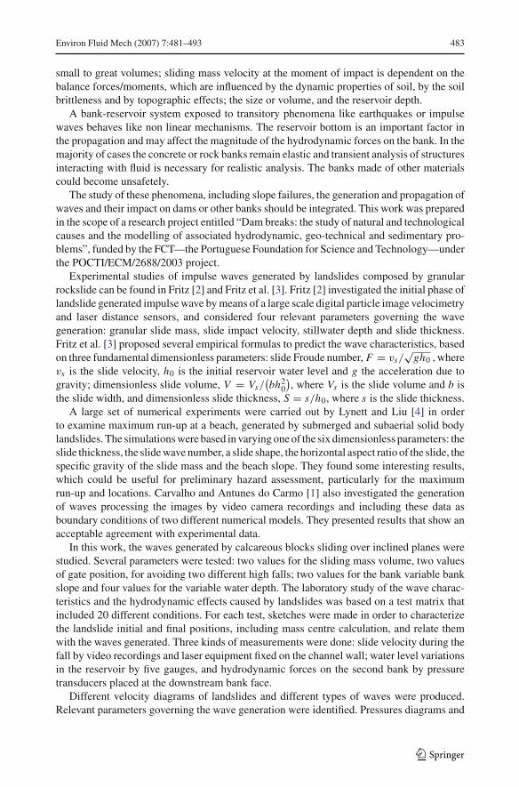
The channel of the laboratory installation is 40.0 m×1.5 m×1.0 m (L×H×W); the variablesloping bank and the dam were placed along a length of approximately 12 m. The landslidewas reproduced in the laboratory installation by calcareous masses that fell by sliding overthe bank. Figure 1 shows a view of the laboratory installation.

Sliding masses were simulated by several calcareous blocks, measuring 10 cm×8 cm×7 cm (L×H×W), and with density ρs/ρ = 2.38 and porosity ηpor ≈ 0.40. Some blocks werecut to accommodate the gate placed to retain the calcareous material before the experiment.The friction angle was determined experimentally by varying the bank slope with the twodifferent volumes placed above it and without any retention. For the two volumes, 0.0814 m3

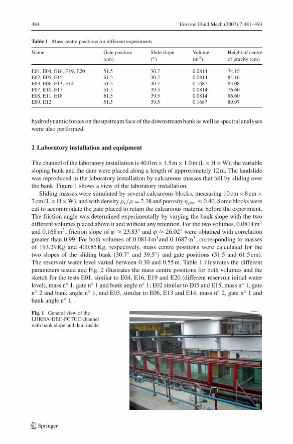
and 0.168 m3, friction slope of φ ≈ 23.83◦ and φ ≈ 26.02◦ were obtained with correlationgreater than 0.99. For both volumes of 0.0814 m3and 0.1687 m3, corresponding to massesof 193.29 Kg and 400.85 Kg, respectively, mass centre positions were calculated for thetwo slopes of the sliding bank (30.7◦ and 39.5◦) and gate positions (51.5 and 61.5 cm).The reservoir water level varied between 0.30 and 0.55 m. Table 1 illustrates the differentparameters tested and Fig. 2 illustrates the mass centre positions for both volumes and thesketch for the tests E01, similar to E04, E16, E19 and E20 (different reservoir initial waterlevel), mass n◦ 1, gate n◦ 1 and bank angle n◦ 1; E02 similar to E05 and E15, mass n◦ 1, gaten◦ 2 and bank angle n◦ 1, and E03, similar to E06, E13 and E14, mass n◦ 2, gate n◦ 1 andbank angle n◦ 1.

Fig. 1 General view of theLHRHA-DEC-FCTUC channelwith bank slope and dam inside

123


Fig. 2 Calculation of the mass centre position: initial position for the tests: E01, E02 and E03

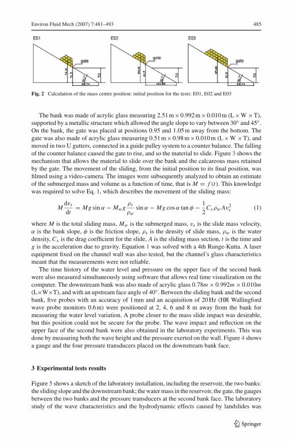
The bank was made of acrylic glass measuring 2.51 m×0.992 m×0.010 m (L×W ×T),supported by a metallic structure which allowed the angle slope to vary between 30◦ and 45◦.On the bank, the gate was placed at positions 0.95 and 1.05 m away from the bottom. Thegate was also made of acrylic glass measuring 0.51 m×0.98 m×0.010 m (L×W ×T), andmoved in two U gutters, connected in a guide pulley system to a counter balance. The fallingof the counter balance caused the gate to rise, and so the material to slide. Figure 3 shows themechanism that allows the material to slide over the bank and the calcareous mass retainedby the gate. The movement of the sliding, from the initial position to its final position, wasfilmed using a video-camera. The images were subsequently analyzed to obtain an estimateof the submerged mass and volume as a function of time, that is M = f (t). This knowledgewas required to solve Eq. 1, which describes the movement of the sliding mass:

Mdvs

dt= Mg sin α − Mwg

ρs

ρw

sin α − Mg cos α tan φ − 1

2Cxρw Av2

s (1)

where M is the total sliding mass, Mw is the submerged mass, vs is the slide mass velocity,α is the bank slope, φ is the friction slope, ρs is the density of slide mass, ρw is the waterdensity, Cx is the drag coefficient for the slide, A is the sliding mass section, t is the time andg is the acceleration due to gravity. Equation 1 was solved with a 4th Runge-Kutta. A laserequipment fixed on the channel wall was also tested, but the channel’s glass characteristicsmeant that the measurements were not reliable.

The time history of the water level and pressure on the upper face of the second bankwere also measured simultaneously using software that allows real time visualization on thecomputer. The downstream bank was also made of acrylic glass 0.78m × 0.992m × 0.010m(L×W×T), and with an upstream face angle of 40◦. Between the sliding bank and the secondbank, five probes with an accuracy of 1 mm and an acquisition of 20 Hz (HR Wallingfordwave probe monitors 0.6 m) were positioned at 2, 4, 6 and 8 m away from the bank formeasuring the water level variation. A probe closer to the mass slide impact was desirable,but this position could not be secure for the probe. The wave impact and reflection on theupper face of the second bank were also obtained in the laboratory experiments. This wasdone by measuring both the wave height and the pressure exerted on the wall. Figure 4 showsa gauge and the four pressure transducers placed on the downstream bank face.

3 Experimental tests results

Figure 5 shows a sketch of the laboratory installation, including the reservoir, the two banks:the sliding slope and the downstream bank; the water mass in the reservoir, the gate, the gaugesbetween the two banks and the pressure transducers at the second bank face. The laboratorystudy of the wave characteristics and the hydrodynamic effects caused by landslides was

123


Fig. 3 View of differentcalcareous blocks, mechanismthat allows the material to slideover the bank and the calcareousmass retained by the gate

based on a test matrix that included 20 different conditions. Table 2 shows the differentparameter values chosen for the experiments.

For all experiments, the images were processed by video recordings and the positionsof the sliding blocks were calculated using Eq. 1. Different velocity diagrams of landslidefall were produced: parabolic (E01–E12, E19 and E20), quasi-linear (E13–E17) and quasi-sinusoidal (E18). Figure 6 shows the variation of the sliding mass velocity during the fallcalculated by Eq. 1 for the essays E01–E08, E10–E12 and E16–E18. Analysing Fig. 6 andTable 2, it can be concluded that sudden descending variations occurred due to the reservoirwater level, which is not deep enough to decelerate the sliding mass. In general, a higherinitial position of the centre of gravity corresponds to a higher initial velocity, and a higherslope corresponds to a more pronounced increase in slide velocity. This slide slope has a great

123


Fig. 4 A gauge for water level measurements and the pressure transducers placed on bank downstream upperface

Fig. 5 Definition sketch of the experiments

0.0

0.5

1.0

1.5

2.0

0 0.1 0.2 0.3 0.4 0.5 0.6 0.7 0.8 0.9 1t (s)

vs(m

/s)

E01 E02 E03 E04(5) E06 E07 E08 E10 E11 E12 E16 E17 E18

Fig. 6 Slide mass velocity diagrams during sliding: Tests E01-08, E10-12; E16-18

123


Table 2 Parameter values fordifferent experiments

Name Slide slope Reservoir Slide Centre of(◦) water level volume (m3) gravity (m)

(m)

E01 30.7 0.5 0.0814 0.74E02 30.7 0.5 0.0814 0.84E03 30.7 0.5 0.1687 0.85E04 30.7 0.55 0.0814 0.74E05 30.7 0.55 0.0814 0.84E06 30.7 0.55 0.1687 0.85E07 39.5 0.5 0.0814 0.77E08 39.5 0.5 0.0814 0.87E09 39.5 0.5 0.1687 0.90E10 39.5 0.55 0.0814 0.77E11 39.5 0.55 0.0814 0.87E12 39.5 0.55 0.1687 0.90E13 30.7 0.5 0.1687 0.85E14 30.7 0.4 0.1687 0.85E15 30.7 0.3 0.0814 0.84E16 30.7 0.3 0.0814 0.74E17 39.5 0.3 0.0814 0.77E18 39.5 0.3 0.0814 0.87E19 30.7 0.4 0.0814 0.74E20 30.7 0.45 0.0814 0.74

influence on the maximum slide mass velocity (see E01 and E07). For the larger angle, themaximum velocity difference becomes visible (E08 and E11). Similar results were observedfor the slide mass volume (E01 and E03). However, the slide mass volume variation couldnot be analyzed separated from the initial position of the mass centre. This parameter is veryimportant both the initial and maximum slide mass velocity (see E01 and E02, E07 and E08,E10 and E11, or E16 and E17). In particular, when the initial water level is low, this parametercauses large slide initial velocity (see E16 and E17). The initial water level position is lessimportant for small bank angles (slide mass velocity variation during the fall is similar inE01-E03). The maximum slide velocity was also determined by the following expressiondeduced from the energy balance between the initial and final positions of the slide:

vsm = √2g�z sin (α − φ) (2)

where vsm is the slide velocity when the mass centre reaches the water surface, �z is the heightof the positions of the mass centre before and after the mass sliding, g is the acceleration due togravity, α is the slide slope and φ is the friction slope. In the majority of the tests, an acceptableagreement with the maximum slide velocity calculated by Eqs. 1 and 2 was observed, exceptfor the lower slide slopes and smaller heights of the centre of gravity. Those differences do notinterfere with the prediction of wave type based on the Froude number for sliding velocity anddimensionless slide thickness proposed by Noda [5]: nonlinear for F = vs/

√gh0 < 4−7.5S;

oscillatory for 4 − 7.5S < F < 6.6 − 8S; solitary for 6.6 − 8S < F < 8.2 − 8S anddissipative for F > 8.2 − 8S. However, when it comes to inflow boundary condition innumerical simulations, these differences are very important [1]. The relevant parametersgoverning slide velocity, and so wave generation, consist of: the mass of the sliding blocks,

123


Fig. 7 Water level measurements (h/h0vs.t (g/h0)1/2) in gauges n◦ 1 to n◦ 5 (2 m, 4 m, 6 m, 8 m and 10 mupstream of the bank slope toe): a) E01; b) E16

the still water level in the reservoir, the slope and the initial position of the mass centre of thesliding blocks.

Concerning the generated wave characteristics, it has to be emphasized that they werebased on values of the first wave amplitude obtained at the first gauge placed 2 m after thesliding bank. Having this in mind, values of ac/h0 are greater than 0.03, all values of ac/Lare greater than 0.006 and the Ursell number is always greater than 1, which confirms thewaves nonlinearity characteristics.

In most of the tests, the maximum wave amplitude was attained for the first wave. However,at gauge number 4, placed 8 m from the bank, the amplitude of the second wave exceededthat of the leading wave in tests E10 and E11 (which correspond to higher bank slope, higherreservoir water levels and smaller volumes). This empathize the importance of the distancebetween the landslide and the bank.

The maximum was observed in E03 and E13 (which correspond to smaller bank slope,higher volumes and smaller reservoir depths), the minimum was observed in E04 (whichcorresponds to smaller bank slope, smaller volume and higher reservoir depth). The maximumnegative wave amplitude was observed for E10 and E11 and the minimum for E16, wherethe wave shows characteristics similar to the solitary wave. The maximum positive waveamplitude has a strong dependence on both the mass (volume) of the sliding mass and theinitial water level. To investigate the influence of the initial water depth, the tests E01, E04,E16, E19 and E20, where the initial water depths are different, were studied in particular.Figure 7 illustrates the water level measurements at the five gauges in tests E01 and E16, and

123


y = -1.9234x2 + 0.719x + 0.3782R2 = 0.973

y = -0.7324x + 0.5653R2 = 0.9885

y = -0.6541x + 0.5038R2 = 0.9942

y = -0.6054x + 0.4684R2 = 0.9913

y = -0.9081x + 0.7076R2 = 0.9467

0

0.1

0.2

0.3

0.4

0.5

0.2 0.3 0.4 0.5 0.6h0 (m)

max

. a (m

)Gauge 1

Gauge 2

Gauge 3

Gauge 4

Poly. (Gauge 1)

Linear (Gauge 2)

Linear (Gauge 3)

Linear (Gauge 4)

Linear (Gauge 1)

Fig. 8 Maximum amplitude variations on gauges 1 to 5 with the initial reservior water level: E01, E04, E16,E19 and E20

-2000

-1000

0

1000

2000

3000

4000

5000

6000

7000

0 5 10 15 20 25 30

t (s)

p (P

a)

estimated by interpolation

Press.transd. 4

Press.transd. 3

Press.transd. 2

Press.transd. 1

Fig. 9 Pressure values on the upstream face of the downstream bank: Test E01

Fig. 8 shows the maximum amplitude variations with the initial reservoir water level between0.30 m and 0.55 m at gauges 1–4 (essays E01, E04, E16, E19 and E20).

Velocity, like the wave amplitude, is also very important for the risk prediction and hazardprevention, i.e. for efficient activation of emergency plans. For non linear waves, as thoseof this work, celerity is strongly dependent on the relative amplitude, ac/h0, wave length,L , and initial water level, h0. Propagation velocity decreases with the amplitude and wavelength. In the present study values in the range 0.9 < ac1/

√gh0 < 1.2 for the first wave

and 0.6 < ac1/√

gh0 < 1.0 for the second one were obtained, which confirm this theory.According to the Boussinesq theory, the following expression for the solitary wave velocityis valid: cc1/

√gh0 = 1 + ac1/(2h0), where 1 refers to the first wave. This expression gives

differences of less than 20% for all tests.Hydrodynamic pressures on the downstream bank face were measured using pressure

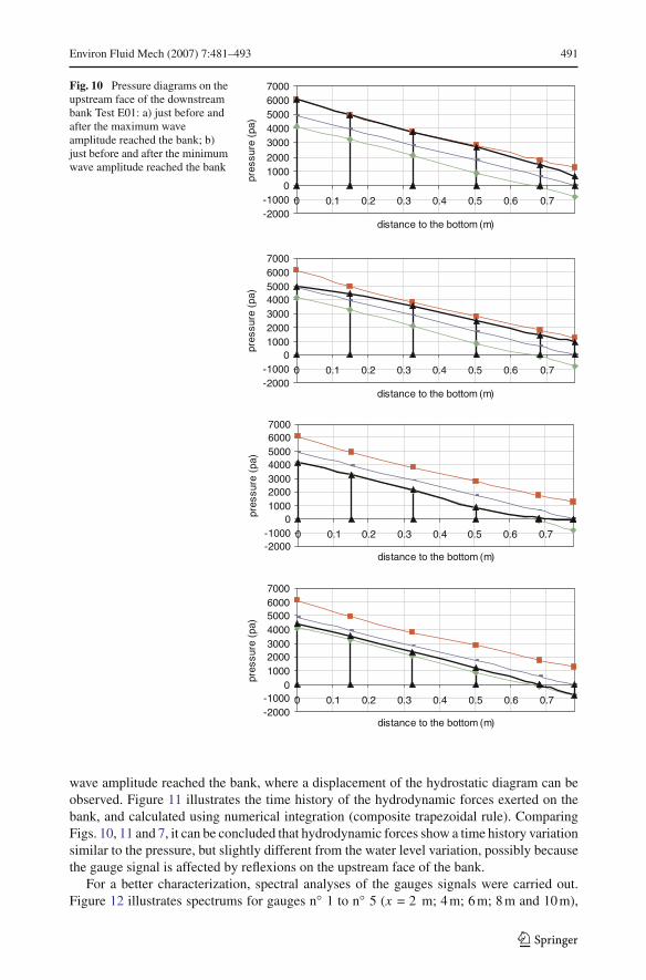
transducers. Instability was observed after a wave reflection upstream at the face of thedownstream bank. Figure 9 illustrates pressure time history values at pressure transducers 1–4.At the bottom and at the top of the bank, the pressure values were estimated using Lagrangeinterpolation. Figure 10 illustrates the pressure diagrams at 4 instants, just before and afterthe maximum wave amplitude reached the bank and just before and after the minimum

123


Fig. 10 Pressure diagrams on theupstream face of the downstreambank Test E01: a) just before andafter the maximum waveamplitude reached the bank; b)just before and after the minimumwave amplitude reached the bank

-2000-1000

010002000

30004000500060007000

0 0.1 0.2 0.3 0.4 0.5 0.6 0.7

distance to the bottom (m)

pres

sure

(pa

)

-2000-1000

01000200030004000500060007000

0 0.1 0.2 0.3 0.4 0.5 0.6 0.7


pres

sure

(pa

)

-2000-1000

01000200030004000500060007000

0 0.1 0.2 0.3 0.4 0.5 0.6 0.7


pres

sure

(pa

)

-2000-1000

01000200030004000500060007000

0 0.1 0.2 0.3 0.4 0.5 0.6 0.7


pres

sure

(pa

)

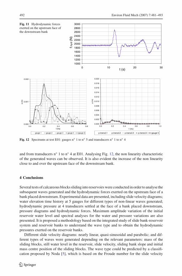
wave amplitude reached the bank, where a displacement of the hydrostatic diagram can beobserved. Figure 11 illustrates the time history of the hydrodynamic forces exerted on thebank, and calculated using numerical integration (composite trapezoidal rule). ComparingFigs. 10, 11 and 7, it can be concluded that hydrodynamic forces show a time history variationsimilar to the pressure, but slightly different from the water level variation, possibly becausethe gauge signal is affected by reflexions on the upstream face of the bank.

For a better characterization, spectral analyses of the gauges signals were carried out.Figure 12 illustrates spectrums for gauges n◦ 1 to n◦ 5 (x = 2 m; 4 m; 6 m; 8 m and 10 m),

123


Fig. 11 Hydrodynamic forcesexerted on the upstream face ofthe downstream bank

1000

12001400

1600

1800

20002200

2400

26002800

3000

0 10 20 30t (s)

f.hyd

(N

)

0.000

0.001

0.002

0.0 0.2 0.4 0.6 0.8f (Hz)

a (m

)

gauge 1 gauge 2 gauge 3 gauge 4 gauge 5

0.000

0.002

0.004

0.006

0.008

0.010

0.012

0.014

0.016

0.018

0.020

0.0 0.2 0.4 0.6 0.8 1.0f (Hz)

a (m

)

p.transd.1 p.transd.2 p.transd.3 p.transd.4 gauge 5

Fig. 12 Spectrums at test E01: gauges n◦ 1 to n◦ 5 and transducers n◦ 1 to n◦ 4

and from transducers n◦ 1 to n◦ 4 at E01. Analysing Fig. 12, the non linearity characteristicof the generated waves can be observed. It is also evident the increase of the non linearityclose to and over the upstream face of the downstream bank.

4 Conclusions

Several tests of calcareous blocks sliding into reservoirs were conducted in order to analyse thesubsequent waves generated and the hydrodynamic forces exerted on the upstream face of abank placed downstream. Experimental data are presented, including slide velocity diagrams;water elevation time history at 5 gauges for different types of non-linear waves generated;hydrodynamic pressure at 4 transducers settled at the face of a bank placed downstream,pressure diagrams and hydrodynamic forces. Maximum amplitude variation of the initialreservoir water level and spectral analyses for the water and pressure variations are alsopresented. It is proposed a methodology based on the integrated study of slide bank-reservoirsystem and reservoir banks to understand the wave type and to obtain the hydrodynamicpressures exerted on the reservoir banks.

Different slide velocity diagrams: nearly linear, quasi-sinusoidal and parabolic; and dif-ferent types of waves were generated depending on the relevant parameters: mass of thesliding blocks, still water level in the reservoir, slide velocity, sliding bank slope and initialmass centre position of the sliding blocks. The wave type could be predicted by a classifi-cation proposed by Noda [5], which is based on the Froude number for the slide velocity

123


(obtained by an expression deduced from the energy balance) and dimensionless slide thick-ness. The maximum positive wave amplitude has a strong dependence on the mass (volume)of the sliding mass and on the initial water level, showing a quasi-linear variation.

More tests results are essential to support correlation and develop formulas able to predictthe wave amplitude, velocity propagation, hydrodynamic pressures and forces. The transientanalysis of the integrated system, slide bank, reservoir and structure bank is necessary forrealistic analysis.

Acknowledgements The authors wish to acknowledge Portuguese Foundation for Science and Technologyunder the project POCTI/ECM/2688/2003, André Pestana for some experimental tests and calculations, andMr. Joaquim Cordeiro, a technician of the LHRHA-DEC-FCTUC.

References

1. Carvalho RF, Antunes do Carmo JS (2006) Numerical and experimental modelling of the generation andpropagation of waves caused by landslides into reservoirs and their effects on dams. In: Ferreira RML,Alves ECTL, Leal JGBA, Cardoso AH (eds) Proc River Flow 2006, vol 1. Lisbon, Portugal, pp 483–492

2. Fritz HM (2002) PIV applied to landslide generated impulse waves. In: Adrian RJ et al (eds) Lasertechniques for fluid mechanics. Springer, New York, pp 305–520

3. Fritz HM, Hager WH, Minor H-E (2004) Near field characteristics of landslide generated impulse waves.J Waterw Port Coastal Ocean Eng 130:287–300

4. Lynett P, Liu PLF (2005) A numerical study of the run-up generated by three-dimensional landslides.J Geophysical Research-Oceans 110(C3):Art. No. C03006 MAR 8 2005

5. Noda E (1970) Water waves generated by landslides. J Waterw Port Coastal Ocean Div Am Soc Civ Eng96(4):835–855

123

landslides into reservoirs and their impacts on banks fluid mech (2007) 7:481–493 485 fig. 2...

Documents