landscape and climate changes influence on …
TRANSCRIPT
PAULA EVELINE RIBEIRO D’ANUNCIAÇÃO
LANDSCAPE AND CLIMATE CHANGES INFLUENCE ON
TAXONOMIC AND FUNCTIONAL RICHNESS OF
AMPHIBIANS
LAVRAS – MG
2018

PAULA EVELINE RIBEIRO D’ANUNCIAÇÃO
LANDSCAPE AND CLIMATE CHANGES INFLUENCE ON TAXONOMIC AND
FUNCTIONAL RICHNESS OF AMPHIBIANS
Prof. Dr. Luis Marcelo Tavares de Carvalho
Orientador
Prof. Dr. Milton Cezar Ribeiro
Coorientador
Prof. Dr. Raffael Ernst
Coorientador
LAVRAS – MG
2018
Tese apresentada à Universidade Federal
de Lavras, como parte das exigências do
Programa de Pós-Graduação em Ecologia
Aplicada, área de concentração em
Ecologia e Conservação de Recursos
Naturais em Paisagens Fragmentadas e
Agroecossistemas, para obtenção do título
de doutor.

Ficha catalográfica elaborada pelo Sistema de Geração de Ficha Catalográfica da Biblioteca
Universitária da UFLA, com dados informados pelo(a) próprio(a) autor(a).
Ribeiro D Anunciação, Paula Eveline.
Landscape and climate changes influence on taxonomic and
functional richness of amphibians / Paula Eveline Ribeiro D
Anunciação. - 2018.
114 p. : il.
Orientador(a): Luis Marcelo Tavares de Carvalho.
Coorientador(a): Milton Cezar Ribeiro, Raffael Ernst.
Tese (doutorado) - Universidade Federal de Lavras, 2018.
Bibliografia.
1. Functional richness of amphibians. 2. Environmental
thrseholds. 3. Climate changes. I. Tavares de Carvalho, Luis
Marcelo. II. Ribeiro, Milton Cezar. III. Ernst, Raffael. IV. Título.

PAULA EVELINE RIBEIRO D’ANUNCIAÇÃO
LANDSCAPE AND CLIMATE CHANGES INFLUENCE ON TAXONOMIC AND
FUNCTIONAL RICHNESS OF AMPHIBIANS
APROVADA em 21 de março de 2018,
Profa. Dra. Cinthia Aguirre Brasileiro
Profa. Dra. Erica Hasui
Dra. Lívia Dorneles Audino
Prof. Dr. Marcelo Passamani
Prof. Dr. Luis Marcelo Tavares de Carvalho
Orientador
LAVRAS – MG
2018
Tese apresentada à Universidade Federal
de Lavras, como parte das exigências do
Programa de Pós-Graduação em Ecologia
Aplicada, área de concentração em
Ecologia e Conservação de Recursos
Naturais em Paisagens Fragmentadas e
Agroecossistemas, para obtenção do título
de doutor.

Dedico esta tese à minha mãe, Jussara, pelo apoio, carinho e incentivo.

AGRADECIMENTOS/ACKNOWLEDGEMENTS
À Universidade Federal de Lavras, especialmente ao Departamento de Biologia e ao
Programa de Pós Graduação em Ecologia Aplicada, pela oportunidade.
À CAPES, pela concessão da bolsa de doutorado no país e também pela bolsa no
exterior processo nº 88881.134118/2016-01.
Ao meu orientador Luis Marcelo “Passarinho” por ter recebido tão bem como orientada,
ainda que com áreas de pesquisa um tanto quanto distintas. Obrigada pela disponibilidade em
ajudar sempre.
Ao meu coorientador Milton Cezar Ribeiro “Miltinho” por também me receber de
braços abertos, possibilitando o desenvolvimento desse trabalho através do financiamento e
logística do campo, infraestrutura do Laboratório de Ecologia Espacial e Conservação (LEEC).
E, principalmente por várias discussões científicas que deram embasamento a essa tese.
Sobretudo, por ensinar a importância das colaborações científicas.
Aos membros da banca que aceitaram o convite e que tenho certeza que trarão
importantes contribuições: Cinthia Brasileiro, Erica Hasui, Lívia Audino e Marcelo Passamani.
E também ao Júlio Louzada e Marco Aurélio, suplentes, mas não menos importantes.
À secretária da Ecologia, Ellen, sempre tão disponível para ajudar e mega eficiente.
Ellen, com certeza essa tese não seria finalizada sem sua ajuda!
Aos queridos amigos conquistados na cidade de Lavras, em duros momentos de
distração, baladas, conversas indispensáveis e claro profissionais: Nay Alecrim, Nath Carvalho,
Mard Ribeiro, André Tavares. Meu muito obrigada em especial ao Fernando Puertas “Java” por
compartilhar imensa parte da minha caminhada no doutorado e por me inspirar a ser uma
cientista mais humana e preocupada com os pares. Ao grande amigo Antônio Queiroz “Toin”,
que chegou de mansin e com jeitin carinhoso, por sempre estar presente, mesmo longe,
dividindo momentos alegres e tristes.
Às amigas de república: Dani, Nayara e Raquel por dividirem momentos tão especiais
regados a boas comidas e cerveja (quente), na minha primeira casa, fora de casa. Dani, mãos de
fada, sempre preocupada com a nossa saúde. Nayara fazendo das nossas vidas mais gostosas,
com comidas maravilhosas, principalmente um macarrão com brócolis! Em especial à amiga
Raquel “xexe, xexelenta”, que desde o começo me identifiquei tanto e que sempre esteve
presente incentivando nos momentos mais difíceis e nos alegres também. Companhia no Brasil
e na Europa, compartilhando experiências que com certeza nunca mais esqueceremos. No mais,
consertos de itens tecnológicos é com a gente mesmo!
Ao barco da Catuaba: Java, André, Tonho, Wallace, Peixe, Ananza, Nath e muitos
outros amigos, que tornou muitos réveillons inesquecíveis.
Aos amigos de Rio Claro, principalmente Carlos Gussoni “Parso”, meu grande amigo,
irmão, sempre presente e companheiro. Amigo que fez da minha estadia em Rio Claro ter um
motivo muito mais belo e sincero do que meramente profissional. Obrigada pelos vários
almoços no bom prato, sempre esperando pela feijoada e por cozinhar tortas maravilhosas.
Ao pessoal do LEEC que gentilmente me receberam. Em especial ao Felipe Martello e
Maurício Vancine que sempre me ajudaram nos tortuosos caminhos do R e também por valiosas
discussões ecológicas e biológicas.
Aos amigos brasileiros que o PDSE me contemplou e fizeram da minha estadia na
Alemanha inesquecível. Aluísio, amigo das viagens maravilhosas, amigo dos momentos mais
loucos na Europa (Martin que o diga), amigo das IPAs, amigo-irmão. Cléber, uma grande
coincidência da vida que permitiu eu conhecer melhor essa pessoa tão especial e fora da
caixinha. Gabi, a moça mais doce e simpática do mundo, obrigada por dividir as inseguranças
da nossa profissão e por tantos conselhos na hora certa.
Aos amigos de Alfenas, família que eu escolhi, tenho o maior orgulho e que não importa
a distância, carrego para sempre no coração. Ane, Jack, Jean, Erick, Ju, Silvia, Wart, Ricardo,
Fernanda, Cabeça.
À minha família, à melhor família do mundo, recheada de mulheres fortes e
inspiradoras. À minha mãe, mulher mais forte que conheço, por ensinar o valor do amor
verdadeiro. Aos irmãos, João e Yago, que dão trabalho, mais que amo infinitamente. Ao irmão
Júnior que me ensinou da forma mais triste que o amor é eterno. Às minhas tias maravilhosas,
minhas mães por escolha, Tia Candinha, Tia Pepê e Tia Cida, sempre presentes. À vó mais
linda, mais amorosa, mais inspiradora, mais corajosa e com certeza a melhor do mundo. Para
sempre meu docinho. Aos tios Wagner e Joãozinho e aos priminhos maravilhosos Amandinha,
Teteu e Tatá.
I am very grateful to the Senckenberg Institute in Dresden, Germany, for the great
opportunity to learn and study abroad. I am even more grateful to Raffael Ernst, my supervisor
in Germany (the best German ever), who was/is always so kind and always available to help
and share his professional experience with me.
I am also very grateful to Melita [the girl from Slovenia] for received me very well, for
be my best friend in Dresden and for always be present whenever I needed. Thank you for the
several nights drinking and talking about life, love, friendship. Thank you for still support me
and for be always nice and concerned. Thank you Ole and Flora for the good moments in

Dresden. Thank you Marko [the lonely guy from Serbia] for help me with R, for be my first
friend in the museum, for went out with me in Dresden, for drink beer sitting on the street, for
share a great musical taste, for the big sense of what science really is, for be annoying sometimes
and for the very good time shared.
Obrigada a todos, essa tese com certeza tem um pouco de cada um dentro dela/Thank
you everyone, this thesis has a little bit of each one inside it.

RESUMO
A supressão de áreas naturais, chamada perda de hábitat, e a implantação de novos usos da terra
leva ao declínio de espécies, extinção em casos extremos e ainda dominância de espécies
generalistas e resistentes ao distúrbio. Além de mudanças no uso da terra, o aumento da
temperatura atmosférica, por si só ou em sinergia com outras perturbações, causa extinção
daquelas espécies incapazes de se adaptar ou se dispersar para locais mais adequados. Anfíbios
apresentam características de história de vida que os deixam particularmente sensíveis às
perturbações provocadas pelo homem. A sensibilidade dos anfíbios às mudanças antrópicas os
tornam modelos ideais para avaliar o impacto, entretanto ainda não é claro a influência dessas
mudanças nos seus atributos funcionais. Os objetivos dessa tese foram: i. determinar a
suficiência amostral de anfíbios de acordo com a proporção de cobertura florestal utilizando
gravadores autônomos; ii. definir os principais preditores ambientais da distribuição de três
componentes de diversidade de anfíbios (espécies, grupos funcionais e traços funcionais) e
identificar limiares ambientais responsáveis pela substituição da comunidade taxonômica ou
funcional; iii. avaliar o efeito das mudanças climáticas na riqueza taxonômica e funcional de
anfíbios ao longo da Mata Atlântica de acordo com dois cenários de aumento de temperatura.
Utilizando gravadores autônomos, uma nova ferramenta de coleta de dados, e complementando
com busca visual a auditiva, determinei a riqueza e composição de anfíbios em cada paisagem
amostral. Os principais resultados foram: i. a suficiência amostral de anfíbios não está
relacionada com a proporção de cobertura florestal; ii. plantação de eucalipto, corpos d’água e
heterogeneidade ambiental são os principais preditores da distribuição dos componentes de
diversidade. Os limiares de substituição de comunidades acontecem no início dos gradientes
ambientais antrópicos, exceto para heterogeneidade ambiental que apresentou o principal limiar
na porção intermediária de seu gradiente. Os diferentes componentes possuem resposta
similares; iii. As mudanças climáticas vão ocasionar perda de espécies e funções, porém a perda
de funções é mais proeminente. A conversão de áreas naturais em gradientes antropogênicos
causa substituição de espécies e funções ainda que represente uma pequena proporção da
paisagem. No entanto, a heterogeneidade ambiental mostra que a presença de diferentes usos
da terra é benéfica para os anfíbios até a porção intermediária do gradiente, já que a combinação
de áreas naturais e antrópicas podem oferecer diferentes recursos. Os cenários de aumento de
temperatura são negativos para os anfíbios, a redundância funcional estará comprometida no
futuro e, tanto a riqueza taxonômica quanto funcional estará restrita principalmente ao sudeste
do Brasil em áreas costeiras. Com relação ao gravadores autônomos, pude indicar um esforço
amostral mínimo, porém ainda é necessário mais estudos para determinar o esforço ideal.
Ambos os impactos antropogênicos acarretam consequências negativas para a comunidade de
anfíbios e os componentes de diversidade apresentam respostas complementares, ainda que
similares em muitos casos.
Palavras-chave: Gravadores autônomos. Limiares ambientais. Anuros. Mata Atlântica.
Aquecimento Global.

ABSTRACT
Deforestation and suppression of natural areas, called habitat loss, and the implementation of
new land uses lead to species decline, extinctions, and dominance of generalist and disturbance-
resistant species. In addition to changes in land use, the temperature increase, either alone or in
synergy with other disturbances, causes extinction of those species unable to adapt or disperse
to suitable places. Amphibians have life history characteristics that make them particularly
sensitive to anthropogenic disturbances. The amphibian sensitivity to anthropogenic changes
makes them ideal models to evaluate the impact, however the influence of these changes on
their functional traits still is not clear. The objectives of this thesis were: i. to determine the
amphibians sampling sufficiency according to the forest cover proportion, using automated
recorders; ii. to define the main environmental predictors of the three components of amphibian
diversity distribution (species, functional groups and functional traits) and to identify
environmental thresholds responsible for the turnover of taxonomic or functional community;
iii. to evaluate the climate changes effect on the taxonomic and functional richness of
amphibians in the Atlantic Forest according to two scenarios of temperature increase. Using
automated recording systems, a new data collect tool, I determined the amphibian richness and
composition in each sampling landscape. The main results were: i. the amphibians sampling
sufficiency is not related to the forest cover proportion; ii. Eucalyptus plantation, water bodies
and environmental heterogeneity are the main predictors of the diversity components
distribution. Thresholds of community turnover occur at the beginning of anthropogenic
environmental gradients, except for environmental heterogeneity that showed the main
threshold at the intermediate portion of its gradient. The different components have similar
responses; iii. Climate changes will cause species loss and functions, but loss of function is
more prominent. The conversion of natural areas into anthropogenic gradients causes species
and function substitution, even though the gradient represents a small proportion of the
landscape. However, environmental heterogeneity shows that the different land uses are
beneficial for amphibians to the intermediate portion of the gradient, since the combination of
natural and anthropic areas may offer different resources. The scenarios of temperature increase
are negative for amphibians, functional redundancy will be compromised in the future, and both
taxonomic and functional richness will be restricted mainly to southeastern Brazil in coastal
areas. Regarding to the automated recording systems, I indicated a minimal sampling effort,
however it is still necessary more studies to determine the ideal sampling effort. Both
anthropogenic impacts have negative consequences for the amphibian community and the
components of diversity present complementary responses, although similar in many cases.
Key-words: Automated recorder systems – Tipping points – Anurans – Brazilian Atlantic
Forest – Global warming.

TABLE OF CONTENTS PRIMEIRA PARTE ................................................................................................................. 12
1 GENERAL INTRODUCTION ............................................................................................. 12
REFERENCES ......................................................................................................................... 14
SEGUNDA PARTE - ARTIGOS ............................................................................................. 18
ARTIGO 1 - Sampling sufficiency using audio recording systems for estimating anuran
diversity……………………………………………………………………………………….18
ARTIGO 2 - Using environmental thresholds to predict taxonomic and functional turnover in
anuran communities of a highly fragmented and threatened forest ecosystem ........................ 34
ARTIGO 3 - Functional and taxonomic amphibian decline due to climate change within
Brazilian Atlantic Forest ........................................................................................................... 87
CONCLUSION ...................................................................................................................... 112

12
PRIMEIRA PARTE
1 GENERAL INTRODUCTION
Anthropogenic activities due to economic growth have severe impact on natural
systems, causing biodiversity loss and population declines worldwide (SODHI et al., 2008).
The main drivers of biodiversity reduction are habitat loss and fragmentation, over-exploitation
of natural resources, invasive species and climate changes (MILLENNIUM ECOSYSTEM
ASSESSMENT, 2005). Of these drivers, habitat loss and fragmentation are one primary cause
(TILMAN et al., 2001), which is true to amphibian populations as well (STUART et al., 2004).
Amphibians are facing worldwide declines, with an estimate of over 160 world species had
already become extinct, and at least 43% of describing species are experiencing population
declines (STUART et al., 2004). In addition, other causes, such as climate changes, might
accelerate the extinction rate (THOMAS et al., 2004). Although the number of studies
evaluating the impact of habitat suppression and modification and global warming to amphibian
diversity and/or richness is increasing (BEEBEE; GRIFFITHS, 2005; LIPS et al., 2005;
BLAUSTEIN et al., 2010; LI et al., 2013), literature about the impact of these threats on other
components of diversity, such as functional diversity, is still scarce (RIBEIRO et al., 2017;
TRIMBLE; VAN AARDE; 2014 2010; ERNST et al., 2006).
Habitat fragmentation is the process where a large area of natural habitat is converted
in smaller patches with a matrix different from the natural habitat, causing isolation between
habitat patches (WILCOVE et al., 1986). Habitat loss is the reduction of the habitat amount
(FAHRIG, 2003). There are several consequences of those processes, such as increase
probability of extinction, decreased species richness and abundance, changes in the species
distribution and composition within habitat patches, as well as a general loss of biodiversity
(BUTCHART et al. 2010; PIKE et al., 2011b; D’CRUZE; KUMAR, 2011). However, the
effects are not uniform among species, whose habitat preferences and the ability to tolerate or
explore modified conditions will determine their persistence and survival (PIKE et al., 2011b;
PELEGRIN; BUCHER, 2012).
As a consequence of habitat loss, fragmentation and anthropogenic activities, different
types of land covers surround the habitat patches, resulting in landscapes formed by a complex
mosaic (RICKETTS, 2001). When anthropogenic matrices replace natural habitats, the
isolation between these habitats increases. At the same time, the type of matrix can change the
predation risk (BIZ et al., 2017). Moreover, depending on matrix structure the permeability of
fauna varies, allowing individuals to use these matrices as a complementary source of resources

13
or alternative habitat (PARDINI, 2004, WATLING, 2011). However, the combination of
natural and cultivated areas can be positive to the biodiversity since can provide different
resources. Recent studies showed this is true to amphibians and the arthropod functional
community (GUERRA; ARÁOZ, 2015; GÁMEZ-VIRUÉS et al., 2015). In addition, Fahrig
(2017) found that –independent of habitat loss – the majority of responses to habitat
fragmentation is positive. However, this finding is related mainly with taxonomic richness, and
this may not be the same for functional or phylogenetic diversity. Therefore, we need to evaluate
the effects of anthropogenic landscape modification in other levels of diversity – such as
functional diversity– in order to fully understand the impact of habitat loss and fragmentation
on biodiversity, ecosystem functions and related ecosystem services (TRIMBLE; van AARDE,
2014; RIBEIRO et al., 2017).
Climate change has also been pointed as having high impact on biodiversity. The 20th
century was the warmest of the last millennium, with the main change occurring in the last 30
years (JONES et al., 2001). In the current century, the near surface temperatures had already
increased 0.5ºC, causing changes in precipitation pattern and increasing the occurrence of
extreme weather events (EASTERLING et al., 2000). In a review about the consequences of
climate change on biodiversity, Daufresne et al. (2009) suggests three main responses: a) range
shifts in geographic distribution; b) changes in phenology and c) reductions of the body size.
Then, species can try to find better conditions moving to cooler regions, or anticipate the
breeding time to avoid extreme temperatures. If movement or adaptation is not successful,
conditions are not suitable anymore leading to the extinction (PETERSON et al., 2005). As an
example, because their sensitivity to the weather conditions, tropical coral reefs and amphibians
are indicated as the animals that will be more affected by climate changes (PARMESAN, 2006).
The high sensitivity of amphibians is due to a set of characteristics. They present a
biphasic life cycle, requiring two different types of habitat to complete the ontogenetic stages
(BECKER et al., 2007). The habitat loss and fragmentation cause a disconnection between these
suitable habitats, leading to a decrease of reproductive events and individual abundance, lastly
species extinction (HARPER et al., 2008; BECKER et al., 2010). The low vagility or movement
capacity and the philopatry make them poor dispersers, and within a hostile matrix the
connection between the habitats are reduced (SINSCH, 1990; BUCKLEY et al., 2012). Habitat
fragmentation and loss in synergism with climate changes can result in worse effects on
amphibians, which can cause population declines, even local and regional extinction of the
more sensitive species (THOMAS et al., 2004). In addition, because amphibians are
ectothermic depending on the external temperatures to regulate their body functions and present
14
a permeable skin to gas exchange (DUELLMAN; TRUEB, 1994), the impact of climate
changes can be even higher (CATENAZZI, 2015).
Regardless what type of anthropogenic activity or what component of diversity are
being considered in the study to evaluate the impact on biodiversity, it is first necessary to
define an effective way to represent the biodiversity. Automated recording systems are a novel
sampling tool that allows collecting data from vocalizing animals and provide a faster and better
estimation of biodiversity with reduced field effort (DORCAS et al., 2009). Other advantages
are the simultaneous sampling in remote and difficult access areas, and permanent record
(HUTTO; STUTZMAN, 2009). In addition, they allow the cross-validation of the data by
different experts, what increases the accuracy of the information (PEREYRA et al., 2017).
However, these recorders can generate a huge amount of data, being a challenge the storage
and data processing (ACEVEDO; VILLANUEVA-RIVERA, 2006). One solution to avoid the
caveats of this technique is to establish a suitable and efficient minimal time recording schedule.
I divided this thesis in five chapters. The first is the currently chapter, a general
introduction. The second one is a methodological study, where I used audio recordings to
determine what is the amphibians sampling sufficiency according the forest cover proportion.
This second chapter provide the raw data to the second one, where I investigate the influence
of different land uses on the distribution of three levels of amphibians’ diversity: a) species; b)
functional groups; and c) functional traits. After finding the best predictors, I analyzed their
anthropogenic environmental gradients to determine where non-linear and rapid changes, called
ecological thresholds or tipping points, happened. In addition, I compared the three levels of
biodiversity responses. In the fourth chapter, I evaluated the influence of climate changes on
amphibians’ taxonomic richness and functional richness across the Atlantic Forest hotspot. I
used data on amphibian communities for generate habitat suitability models according two
different scenarios of climate change. Finally, the last chapter is a general conclusion of the
thesis.
REFERENCES
ACEVEDO, M. A., VILLANEUVA-RIVERA, L. J. Using automated digital recording systems
as effective tools for the monitoring of birds and amphibians. Wildlife society bulletin, v. 34,
n. 1, p. 211–214, 2006.
BECKER, C. G. et al. Habitat split and the global decline of amphibians. Science, v. 318, p.
1775–1777, 2007.

15
BECKER, C. G. et al. Habitat split as a cause of local population declines of amphibians with
aquatic larvae. Conservation Biology, v. 24, p. 287–294, 2010.
BEEBEE, T. J. C., GRIFFITHS, R. A. The amphibian decline crisis: a watershed for
conservation biology? Biological Conservation, v. 125, p. 271–285, 2005.
BIZ, M., CORNELIUS, C., METZGER, J. P. Matrix type affects movement behavior of a
Neotropical understory forest bird. Perspectives in Ecology and Conservation, v. 15, n. 1, p.
10-17, 2017.
BLAUSTEIN, A. R. et al. Direct and indirect effects of climate change on amphibian
populations. Diversity, v. 2, p. 281- 313, 2010.
BUCKLEY, L. B., HURLBERT, A. H., JETZ, W. Broad-scale ecological implications of
ectothermy and endothermy in changing environments. Global Ecology and Biogeography,
v. 21, n. 9, p. 873–885, 2012.
BUTCHART, S. H. Global Biodiversity: Indicators of Recent Declines. Science, v. 328, n.
5982 p. 1164-1168, 2010.
CATENAZZI, A. State of the World's Amphibians. Annual Review of Environment and
Resources, v. 40, n. 1, p. 91-119, 2015.
DAUFRESNE, M., LENGFELLNER, K.; SOMMER, U. Global warming benefits the small in
aquatic ecosystems. PNAS, v. 106, p. 12788–93, 2009.
D’CRUZE, N.; KUMAR, S. Effects of anthropogenic activities on lizard communities in
northern Madagascar. Animal Conservation, v. 14, p. 542–552, 2011.
DORCAS, M.E. et al. Auditory monitoring of anuran populations. In: Amphibian Ecology
and Conservation (ed. C. K. Dodd) Oxford: Oxford University Press, 2010. 556 p.
DUELLMAN, W. E.; TRUEB, L. Biology of Amphibians. Baltimore: The Johns Hopkins
University Press, 1994.
EASTERLING, D. R. et al. Observed climate variability and change of relevance to the
biosphere. Journal of Geophysical Research, v. 105, n. 20, p. 101–114, 2000.
ERNST, R.; LINSENMAIR, K. E.; RODEL, M. O. Diversity erosion beyond the species level:
dramatic loss of functional diversity after selective logging in two tropical amphibian
communities. Biological Conservation, v. 133, p. 143-155, 2006.
FAHRIG, L. Effects of habitat fragmentation on biodiversity. Annual Review of Ecology and
Systematics, v. 34, p. 487-515, 2003.
FAHRIG, L. Ecological responses to habitat fragmentation per se. Annual Review of Ecology,
Evolution, and Systematics, v. 48, p 1-23, 2017.
GÁMEZ-VIRUÉS, S. et al. Landscape simplification filters species traits and drives biotic
homogenization. Nature Communications, v. 6, n. 8568, 2015.

16
GUERRA, C.; ARÁOZ, E. Amphibian diversity increases in a heterogeneous agricultural
landscape. Acta Oecologica, v. 69, p. 78-86, 2015.
HARPER, E. B., RITTENHOUSE, T. A. G., SEMLITSCH, R. D. Demographic Consequences
of Terrestrial Habitat Loss for Pool-Breeding Amphibians : Predicting Extinction Risks
Associated with Inadequate Size of Buffer Zones. Conservation Biology, v. 22, p. 205–1215
2008.
HUTTO, R. L., STUTZMAN, R. J. Humans versus autonomous recording units: a comparison
of point-count results. Journal of Field Ornithology, v. 80, p. 387–398, 2009.
JONES, P. D., OSBORN, T. J.; BRIFFA, K. R. The evolution of climate over the last
millennium. Science, v. 292, p. 662–667, 2001.
LI, Y., COHEN, J. M., ROHR, J. R. A review and synthesis of the effects of climate change on
amphibians. Integrative Zoology, v. 8, p. 145-161, 2013.
LIPS, K. R. et al. Amphibian declines in Latin America: widespread population declines,
extinctions, and impacts. Biotropica, v. 37, p. 163–165, 2005.
MILLENNIUM ECOSYSTEM ASSESSMENT. Ecosystems and human well-being:
biodiversity synthesis. Washington, DC: World Resources Institute, 2005.
PARDINI, R. Effects of forest fragmentation on small mammals in an Atlantic Forest
landscape. Biodiversity and Conservation, v. 13, n. 2567, 2004.
PARMESAN, C. Ecological and Evolutionary Responses to Recent Climate Change. Annual
Review of Ecology, Evolution and Systematics, v. 37, p. 637-669, 2006.
PELEGRIN, N.; BUCHER, E. H. Effects of habitat degradation on the lizard assemblage in the
Arid Chaco, central Argentina. Journal of Arid Environments, v. 79, p. 13–19, 2012.
PETERSON, A. T. et al., Modeling distributional shifts of individual species and biomes. In:
LOVEJOY, T. E.; HANNAH, L. (Orgs.). Climate Change and Biodiversity. New Haven:
Yale University Press, 2005, p. 211 – 228.
PEREYRA, L. C. et al. Diurnal? Calling activity patterns reveal nocturnal habits in the
aposematic toad Melanophryniscus rubriventris. Canadian Journal of Zoology, v. 94, p. 497-
503, 2016.
PETERSON, A. T. et al. Ecological niches and geographic distributions. Monographs in
population biology 49. Princeton, NJ: Princeton University Press, 2011.
PIKE, D. A.; WEBB, J. K.; SHINE, R. Removing forest canopy cover restores a reptile
assemblage. Ecological Applications, v. 21, p. 274–280, 2011b.
RIBEIRO, J. et al. Evidence of neotropical anuran community disruption on rice crops: a
multidimensional evaluation. Biodiversity and Conservation, v. 26, n. 14, 3363-3383, 2017.

17
RICKETTS, T. H. The matrix matters: effective isolation in fragmented landscapes. The
American Naturalist, v. 158, p. 87-99, 2001.
SINSCH, U. Structure and dynamics of a natterjack toad metapopulation (Bufo calamita).
Oecologia, v. 90, p. 489–499, 1992.
SODHI, N. S. et al. Measuring the meltdown: drivers of global amphibian extinction and
decline. Plos one, v. 3, p. 1–8. 2008
STUART, S. N. et al. Status and trends of amphibian declines and extinctions worldwide.
Science, v. 306, p. 1783–1786, 2004.
THOMAS, C. D. et al. (2004) Extinction risk from climate change. Nature, v. 427, p. 145–148,
2004.
TILMAN, D. Functional diversity. In: Encyclopedia of Biodiversity (ed. Levin, S.A.). San
Diego, CA: Academic Press, pp. 109–120, 2001.
TRIMBLE, M. J.; VAN AARDE, R. J. Amphibian and reptile communities and functional
groups over a land-use gradient in a coastal tropical forest landscape of high richness and
endemicity. Animal Conservation, v. 175, p. 441-453, 2015.
WATLING, J. I. Meta-analysis reveals the importance of matrix composition for animals in
fragmented habitat. Global Ecology and Biogeography, v. 20, p. 209–217, 2011.
WILCOVE, D. S., MCCLELLAN, C. H.; DOBSON, A. P. Habitat fragmentation in the
temperate zone. In: SOULE, M.E. (Org.). Conservation biology: the science of scarcity and
diversity. Sunderland: Sinauer Associates, 1986, p. 237-256.

18
SEGUNDA PARTE - ARTIGOS
ARTIGO 1 - Sampling sufficiency using audio recording systems for
estimating anuran diversity
Format based on the guidelines of “Ecological Indicators”

19
Sampling sufficiency using audio recording systems for estimating anuran diversity
Paula Ribeiro Anunciação 1,2,*; Felipe Martello 3; Luis Marcelo Tavares Carvalho1;
Milton Cezar Ribeiro2
¹ Biology Department, UFLA – Universidade Federal de Lavras, 37200-000, Lavras,
Minas Gerais, Brazil
2 Bioscience Institute, UNESP - Universidade Estadual Paulista, Rio Claro,
Department of Ecology, Spatial Ecology and Conservation Lab (LEEC), 13506-900 Rio
Claro, São Paulo, Brazil
3 Department of Environmental Sciences, UFSCAR - Universidade Federal de São
Carlos, P.O. Box 676, 13565-905 São Carlos, São Paulo, Brazil
* corresponding author: [email protected]
ABSTRACT
The selection of suitable conservation areas and the reduction of species loss require accurate
characterization of biodiversity, which depends on efficient sampling methods. Automated
recording systems (ARS) arise as a new tool to improve and to facilitate sampling and
monitoring species that generate acoustic signals. However, ARS produce huge datasets, which
are time demanding for processing and depend on expert knowledge for efficiently
characterizing biodiversity. Moreover, the amount of audio data that is necessary to process is
unknown to many taxa, particularly amphibians. In this study, we aim to answer two questions:
1) what is the minimum recording time needed to accurately estimate amphibian species
richness? 2) does the total area covered by forest in the surroundings of the recording location
influence the minimum recording time? We sampled amphibians using ARS in 10 streams
within the Brazilin Atlantic Forest across different amounts of forest cover. From 208,260
recorded minutes, we randomly choose 3,190 to be listen. We constructed richness
accumulation curves to define the sampling sufficiency, i.e. richness achieves the asymptote.
Regional species richness was 11, and varied from 3 to 9 among landscapes. The needed time
was very variable (min= 70, max=770 minutes). We also found no correlation between the
minimum time of audio processing and forest cover. To facilitate future studies using automated
recorder systems and to ensure a good representation of the community we recommended to
record 770 minutes, which it was our maximal time to reach the amphibians sampling
sufficiency. In addition, in the end of this work we have also proposed a research agenda to
guide next studies about the topic.

20
KEY WORDS
Anura - Survey methods – Acoustic surveys – Soundscape – Bioacoustics
2.1 Introduction
Conservation decisions and species management are commonly based on biodiversity
patterns, which are accessed by all sorts of monitoring techniques. The sampling method and
effort play an important role on conservation programs and ecological studies (Kenkel et al.
1989). Hence, for an effective and accurate sample of a population or community, it is necessary
to use a sampling scheme that ensures a good representation of local or regional biodiversity
(Gotelli and Colwell, 2001; Koblitz et al., 2017). There is a tendency in ecological studies to
enlarge the spatio-temporal range of observations in order to increase our knowledge on
biodiversity patterns (Acevedo and Villanueva-Rivera, 2006). However, by increasing the
sampling effort, biodiversity surveys might become prohibitively expensive and time
consuming. Therefore, studies concerning reasonable sampling efforts are essential to meet a
good balance between survey time, cost and the proper characterization of biodiversity patterns.
For vocalizing species such as birds, frogs, primates and insects, Automated Recording
Systems (ARS) arise as a less costly alternative when compared to traditional sampling
methods, since they provide faster and better estimation of biodiversity with reduced field effort
(Dorcas et al., 2009). The approach consists in using audio recorders to detect species that
generate acoustic signals, enabling data collection continuously (Blumstein et al., 2011).
Although ARS have been already used as a complementary survey technique for a couple of
decades (Parris et al,. 1999, Mack and Alonso, 2000; Montambault and Missa, 2002), they arise
nowadays as a major sampling technique on biodiversity studies worldwide (Acevedo and
Villanueva-Rivera, 2006; Bardeli et al., 2010; Blumstein et al., 2011; Wimmer et al., 2013).
ARS offer advantages on biodiversity monitoring, such as a facilitated survey of remote and
difficult access areas (Hutto and Stutzman, 2009) and a reduced time spent in field campaigns,
due to the possibility of simultaneous sampling. Besides, it guarantees permanent records for
long term studies of many organisms that vocalize, providing key information to support
conservation and mitigation measures (Acevedo and Villanueva-Rivera, 2006). The collected
raw data – i.e. the sound records – can be shared with independent experts, allowing cross-
validation and reducing species identification errors (Pieretti et al., 2015; Willacy et al., 2015;
Pereyra et al., 2017). Moreover, there is less human interference on animal behavior during data
collection, reducing the environmental impact of the sampling process (Digby et al., 2013).

21
ARS also allow researchers to develop studies about soundscape ecology, a new and
emergent investigation field (Farina, 2014). In addition to assess biodiversity richness and
ecological integrity, the audio recordings are a valuable tool to better understand anthropogenic
disturbances, such as land use modifications and climate changes (Liu et al., 2007; Pijanowski
et al., 2011). Soundscape analyses allow the investigation about the complexity of signs and
codes – the biosemiotic relationships – that vocal animals use to communicate with animals
living in the neighborhood (Farina and Pieretti, 2013). However, this monitoring method may
produce a huge amount of data, particularly if sampling is conducted continuously and for many
sites, which requires large capacity storage systems and a substantial expert time to process the
recordings by visually inspecting spectrograms or even listening the audio files (Rempel et al.,
2005, Acevedo and Villanueva-Rivera, 2006). Automatic species detection and classification
software offer efficient methods to process massive datasets, but using these tools when
working with more than a couple of species reduces species classification accuracy (Brandes,
2008, Bardeli et al., 2010). Therefore, the time needed to meet a good balance between audio
processing effort and sampling efficiency is still unknown for many taxa worldwide.
Amphibians are among the most diverse vertebrate in tropical ecosystem, however they
are facing population declines worldwide (Alford and Richards 1999; Stuart et al., 2004;
Skerratt et al. 2007; Blaustein et al., 2010), particularly in the Neotropics (Cortés-Gomes et al.,
2015). These animals are sensitive to habitat change, as they may present biphasic life cycle
being dependent on aquatic environmental to reproduce and terrestrial habitat in the adult phase
(Becker et al., 2007; Becker et al., 2010). Due to this dependency of more than one suitable
area, the majority of species shows a positive correlation with forest cover area, using forests
as nonbreeding habitat or as areas that allow the movement between wetlands (Houlahan and
Findlay, 2003). Then, because of the strong forest-dependency, their importance to ecosystem
functions, as well as its high sensitivity to human impact, amphibians are commonly used as
bioindicators of habitat disturbance (Storfer, 2003; Buckley et al., 2012). However, to access
this important role as bioindicators is necessary to select accurate sampling methods, which
allow good representation of community consequently indispensable information to guide
mitigation and conservation measures.
In this study, we uses ARS data in order to find a less demanding method to identify
amphibian richness derived from large recording datasets. The amphibian vocalizations were
recorded at streams that cross native forest remnants. Ten study sites were selected in the
Atlantic Forest Biome, within the state of São Paulo, Brazil. We aimed at answering the
following questions: a) what is the minimum recording time needed to have an accurate estimate

22
of amphibian species richness at both, landscape and regional levels? b) does the total area
covered by forest in the surroundings of the recording location influence the minimum
recording time? We hypothesized that each landscape will reach the richness asymptote at
different times. Thus, we believe that these times will be positively correlated with the
proportion of forest cover –the greater the amount of forest cover, the richer is the landscape
and, consequently, the higher the time needed to reach the asymptote (Fig. 1).
Figure 1. A. We expected each site with different forest cover will reach the asymptote or the sampling
sufficiency at different times. B. The amount of time to reach the asymptote will be positive correlated
with forest cover.
2.2 Material and Methods
2.2.1 Study Area
The study region comprises the Cantareira-Mantiqueira continuum in the State of São
Paulo, Brazil. We selected 10 permanent streams inside forest patches. All selected streams
were less then 5 m wide, with low water flux and had the presence of aquatic and riparian
vegetation. We defined circular plots with a radius of one kilometer centered at each sampling
point for land cover classification. This dimension was defined based on the average
displacement for amphibians (Guerry and Hunter, 2002; Wagner et al., 2014). In addition, this
has been the scale of response effect of landscape variables on anuran occupancy and diversity
on previous studies (Guerry and Hunter, 2002; Van Buskirk, 2005). Forest cover within the
plots ranged between 20% and 70%. The distance between streams varied between 2.9 and 56
km (average 27 km), and the elevation varied from 846 to 926 m.a.s.l. Many of the forest
remnants are in the intermediate stage of succession (Ribeiro et al., 2009).

23
We visually interpreted high spatial resolution images available in the Basemap Layer
extension of ArcGIS 10 at 1:5,000 geographic scale. Afterwards, we generated land cover maps
for each area and calculated percentage forest cover using the LSMetrics software –
https://github.com/LEEClab/LS_METRICS (Martello et al. in prep). These maps constitute the
landscapes for further analyses.
2.2.2 Data Sampling and Species Identification
We simultaneously installed one audio recorder in each of the 10 landscapes. The Song
Meter SM3 (Wildlife Acoustics, Inc.) were placed at 1.5 m high on trees, which were located
no more than 3 m away from the streams. We set them up to continuously record data from
6:30 PM until midnight with 48 HZ frequency, being stored as uncompressed “.wav” format,
on files of 20 min each. We deployed with four 32 GB SD memory cards plus four D-cell
alkaline batteries and two built-in acoustic microphones. At every 15 days, we replaced the
memory cards and batteries. We conducted the survey during the breeding season, more
specifically between December 2015 and March 2016.
For each landscape, we randomly selected blocks of 10-minutes each as a representative
sample of soundscape. Each block was composed by 10 continuous one-minute randomly
selected audio recording. Although we used blocks of 10-minutes for extract the audios, we
considered every minute as a sampling unit. P.R. Anunciação identified the species of
amphibian from their specific calls with the aid of Raven Pro version 1.4 software (Bioacoustics
Research Program, 2014).
We used the audio data to construct species accumulation curves and to determine the
asymptote point by visual inspection. We defined the optimum interval of processing as the
point at which the curve reaches the asymptote (i.e. the plateau). The number of minutes that
we processed for each landscape depended on the time of asymptote, which varied between 70
to 770 minutes, in a total of 3,190 processed minutes (Table 1). In addition, we used the total
sum of minutes and of species richness to construct a regional accumulation curve.
We used the software R with the iNEXT package (Hsieh et al., 2016) to construct
accumulation curves. We managed the audio data with TuneR package (Ligges et al., 2016).
To evaluate whether the forest cover affects amphibian detection we performed a linear model
wherein the time to reach the asymptote was the response variable and forest cover the
predictor, and we considered a significant relation when p value was lower than 0.05.

24
2.3 Results
We recorded 208,260 minutes (c.a. 3,471 hours) using the ARS. From this amount, we
processed a total of 3,190 min, which varied among landscapes (min=70; max=770 min.).
However only in 2,065 min (64.7%) there was amphibian vocalization (Table 1). The
amphibian species richness per landscape varied between three and nine species, and 11 species
composed the regional pool on our recordings. The species accumulation curve of the total
processed minutes or the regional species accumulation curve confirm that 770 min is enough
to accurately estimate biodiversity (Fig. S21 - Supplementary material 1).
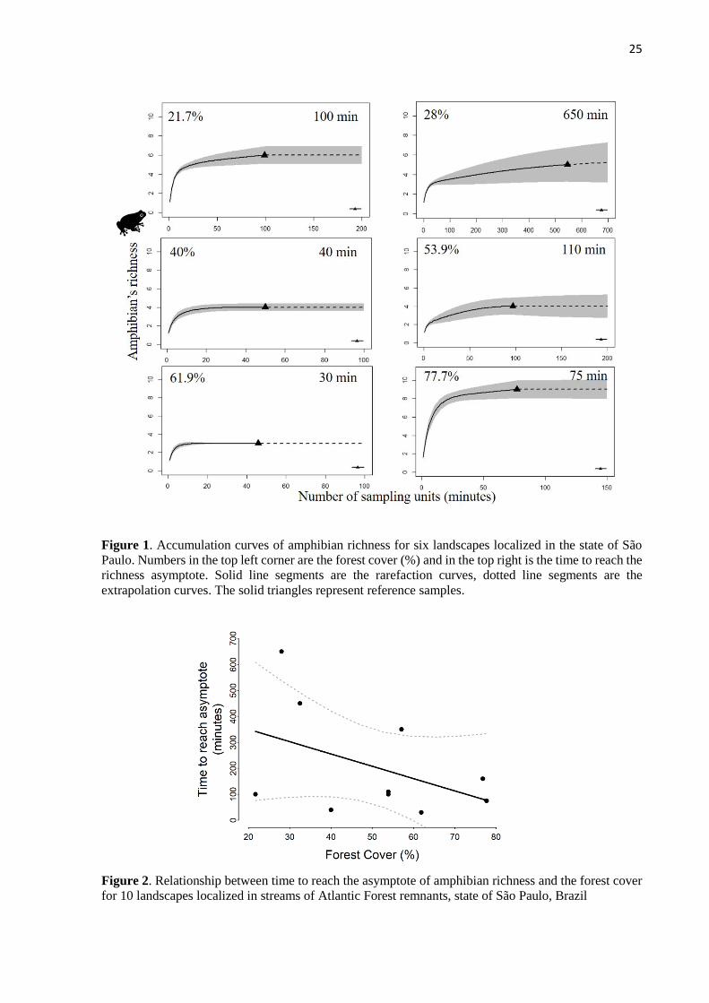
By analyzing the accumulation curves for each landscape, we observed that the time
needed to reach the asymptote varied between 30 and 650 min (s.d. = 207). In Figure 1 we
present the accumulation curve for six out 10 landscapes, where we indicated both the forest
cover and the asymptote.
Regarding the second question, which aimed to evaluate if the amount forest influences
the time needed to reach the asymptote, the relationship was not significant (R²= 0.20, p= 0.20,
Figure 2).
Table 1. Audio recording total sampling effort, minutes processed and accumulation curves’ summary
of 10 sites with different proportion of forest cover. S= amphibian richness, min= minutes, values with
* in the last column means sites that reached the asymptote with estimators.
Forest cover (%) S Sampling effort (min) Processed (min) Asymptote (min)
21.7 6 7410 590 100
28 5 24180 770 650*
32.5 4 21840 460 450*
40 4 22620 70 40
53.9 4 22230 340 110*
53.9 4 22230 140 100
57.1 8 21450 340 350*
61.9 3 22230 70 30
76.8 5 21450 160 160
77.7 9 22620 250 75
Total 11 208260 3190 2065
25
Figure 1. Accumulation curves of amphibian richness for six landscapes localized in the state of São
Paulo. Numbers in the top left corner are the forest cover (%) and in the top right is the time to reach the
richness asymptote. Solid line segments are the rarefaction curves, dotted line segments are the
extrapolation curves. The solid triangles represent reference samples.
Figure 2. Relationship between time to reach the asymptote of amphibian richness and the forest cover
for 10 landscapes localized in streams of Atlantic Forest remnants, state of São Paulo, Brazil

26
2.4 Discussion
Improved data collection is important to implement accurate and cost-effective
surveying programs (Willacy et al., 2015). ARS represent a sampling method that may facilitate
field surveys and provide more accurate data about animals that emit acoustic signals. In this
study, we indicate an appropriate sampling duration time to help improving data collection
when using ARS. This study represents one of the first guidelines for soundscape in a tropical
threatened area. Considering our first research question, we found that each landscape needed
different durations of audio listening time to reach the asymptote, which confirm our first
hypothesis. However, differently from what we expected in the second research question, we
found no correlation between the time that richness reached the asymptote and forest cover.
Our findings, instead of corroborating with the island biogeography theory (MacArthur
and Wilson, 1963) and with the habitat diversity hypothesis (Zimmerman and Bierregaard,
1986), seem to agree with Hill et al. (1994). They have found that the sampling effect can mask
ecological processes. If the sampling effect is removed, the correlation between species number
and area is lower. In our study, we installed one audio recorder in each landscape, independently
of the forest cover area, avoiding oversampling larger areas or subsampling smaller ones. Our
low correlation is probably the result of the variance explained by the real species-area
relationship, as well as other environmental factors that can influence the distribution of
amphibian. It is worth to point out that acoustic sampling has its own limitations. Weather
conditions like storms and wind produce sounds that might interfere the recorded audio and
mask the vocalizations (Towsey et al., 2104; Pieretti et al., 2015). Furthermore, ARS has a
lower sensitivity when compared to human listeners (Hutto and Stutzman, 2009), being more
efficient to detect loud vocalizations in detriment to the quiet ones (Hsu et al., 2005). In
addition, the majority of species vocalize together in the beginning of the night, a phenomenon
called chorus that might hampers species identification (Brandes, 2008).
2.4.1 Sampling sizes effects on amphibian richness
Comparing the amphibian richness found in this study with others in the same region,
we get similar or even greater species richness. Studies in the Atlantic Forest biome using active
search inside forest patches found up to six species (Sabbag and Zina, 2011; Costa et al., 2013;
Maffei et al., 2015), while our study results in three to nine species. We have not found a
correlation between effort time to reach the asymptote and forest cover, which has advantages
and disadvantages. On the one hand, for studies concerning amphibians within forest
ecosystem, such as the Atlantic Forest, we have shown that 770 minutes of audio listening

27
would be enough for using ARS sampling. On the other hand, assuming 770 minutes as the
minimum means that in some cases we are making 10 times more effort compared to the
minimal time found in this study needed to reach the asymptote. One possible explanation to
the lack of correlation between the time to reach the asymptote and forest cover is that other
environmental variables may be more important to explain the patterns. This includes historical
effects of landscape change (Hecnar et al., 1998; Jordan et al., 2009; Zellmer; Knowles, 2009,
Silva et al., 2014) and management practices associated with anthropogenic land use (Skole
and Tucker, 1993). This spatio-temporal dynamics of landscape structure can have potential
effects that will be only detected years later, which is known as the time-lagged response (Ernst
et al., 2006; Metzger et al. 2009; Zellmer; Knowles, 2009).
Another possible explanation is that amphibian’s distribution and abundance can be
attributed to fine spatial scale variables (Parris et al. 2004; Urbina-Cardona et al., 2006; Rojas-
Ahumada et al., 2012). We standardized some variables such as stream width, water flux and
presence of riparian vegetation; however, other variables like understory density, leaf litter
cover and physical structure of the habitat and temperature are examples of important
determinants of amphibian diversity (Ernst et al., 2006; Parris et al., 2004; Urbina-Cardona et
al., 2006; Rojas-Ahumada et al., 2012). Besides, biotic process such as competition, predation,
dispersal, disturbance and disease can also influence the distribution and abundance of
amphibians (Parris et al., 2004; Rojas-Ahumada et al., 2012).
2.4.2 Sampling effort on audio data: standardize or not?
To determine a reliable distribution and abundance of amphibians it is common to
standardize the sampling effort in auditory surveys of amphibians. USA and Canada researchers
defined a standardized survey protocols used by the North American Amphibian Monitoring
Program (NAAMP), which are five minutes in duration at each point of roadside next to
breeding sites (Weir, 2005). Gibbs (2005) recommends a one-minute survey, Crouch and Paton
(2002) and Pierce and Gutzwiller (2004) proposed 10-15 min to a complete survey or to detect
at least 90% of amphibian species. In Brazil, it is common to perform auditory surveys starting
at sunset, ending at midnight (Benício and Silva, 2017; Maffei et al., 2015; Campos et al., 2013;
Zina et al., 2012), which means 6 hours in total. Therefore, there is a lack of standardization of
samplings of biodiversity, and we do need to look for new systems to improve amphibian
sampling. However, it is always necessary to account for the environmental specificities. The
great advantage of ARS in this case is the possibility to increase the survey without fieldwork

28
returns, which can contribute to more accurate biodiversity estimate and a cost-effective
monitoring tool as well (Acevedo and Villanueva-Rivera, 2006; Dorcas et al., 2009).
2.4.3 A research agenda for ARS and sampling sizes
Development of new protocols: more research is necessary in order to determine
protocols for data collection in different environments and different species (or
communities). A standardized data collection method could improve the quality of the
studies, as well as the comparability among them;
Study about the influence of covariates: to find the right protocol is fundamental to
uncover the impact of certain environmental variables on sound recordings, such as
storm, thunders, running water. Also, continuous sounds generate by cicadas and
crickets for example. Anthropogenic sounds are important to considerate as well,
vehicles on roads, engines, bells, sirens can have a huge effect in the quality of the
recordings and disturb the species identification;
Control over the forest cover area variable: we have shown in this study that forest cover
has low correlation with the sampling sufficiency of amphibians. However, by fixing
this variable it would be possible to access the effects of the environmental
heterogeneity within the surroundings;
Development of improved automatic detection algorithms: continuously develop more
efficient algorithms in order to decrease the time spent by experts to filter the recordings,
as well as helping to provide more reliable data, without human bias.
2.5 Conclusion
By assessing the sampling sufficiency, this paper provides a less time-demanding
recording schedule to sampling amphibians in fragmented landscapes. Although we do not find
a correlation between the listened minutes to reach richness asymptote and forest cover, we
could indicate a minimal sampling effort which can reduce costs with batteries, data storage
and expertise time. Because funding is a caveat in ecological researches, sampling techniques
that allow more efficient and accurate population monitoring is indispensable to ensure the
effectiveness of management and conservation strategies (Willacy et al., 2015).
REFERENCES
Acevedo, M.A., Villaneuva-Rivera, L.J. 2006. Using automated digital recording systems as
effective tools for the monitoring of birds and amphibians. Wildlife Soc. B. 34 (1), 211–214.
29
Alford, R.A., Richards, S.J. 1999. Global amphibian declines: a problem in applied ecology.
Annu. Rev. Ecol. Syst. 30, 133-65.
Bardeli, R.,Wolff, D., Kurth, F., Koch,M., Tauchert, K.H., Frommolt, K.H. 2010. Detecting
bird sounds in a complex acoustic environment and application to bioacousticmonitoring.
Pattern Recogn. Lett. 31, 1524–1534.
Becker, C. G., Fonseca, C.R., Haddad, C.F.B., Batista, R.F., Prado, P.I. 2007. Habitat split and
the global decline of amphibians. Science 318, 1775–1777.
Becker, C. G.; Fonseca, C.R.; Haddad, C.F.B.; Prado, P.I. 2010. Habitat split as a cause of local
population declines of amphibians with aquatic larvae. Conserv. Biol. 24, 287–294.
Benício, R.A.; Silva, F.R. 2017. Amphibians of Vassununga State Park, one of the last remnants
of semideciduous Atlantic Forest and Cerrado in northeastern São Paulo state, Brazil. Biota
Neotrop. 17(1), e20160197.
Bioacoustics Research Program. 2014. Raven Pro: Interactive Sound Analysis Software
(Version 1.5) [Computer software]. Ithaca, NY: The Cornell Lab of Ornithology. Available
from http://www.birds.cornell.edu/raven.
Blaustein, A.R., Walls, S.C., Bancroft, B.A., Lawler, J.J., Searle, C.L., Gervasi S.S. 2010.
Direct and indirect effects of climate change on amphibian populations. Diversity 2, 281-
313.
Blumstein, D.R., Mennhil, D.J., Clemins, P. 2011. Acoustic monitoring in terrestrial
environments using microphone arrays: applications, technological considerations and
prospectus. J. Appl. Ecol. 48, 758–67.
Brandes, S.T. 2008. Automated sound recording and analysis techniques for bird surveys and
conservation. Bird Conserv. Int. 18, 163–173.
Buckley, L.B., Hurlbert, A.H., Jetz, W. 2012. Broad-scale ecological implications of
ectothermy and endothermy in changing environments. Global Ecol. Biogeogr. 21, 873–885.
doi:10.1111/j.1466-8238.2011.00737.x
Campos, V. A., Oda, F. H., Juen, L., Barth, A., Dartora, A. 2013. Composição e riqueza de
espécies de anfíbios anuros em três diferentes habitats em um agrossistema no Cerrado do
Brasil central. Biota Neotrop. 13, 124–132.
Cortés-Gómez, A.M., Ruiz-Agudelo, C.A., Valencia-Aguilar, A., Ladle. R.J. 2015. Ecological
functions of neotropical amphibians and reptiles: a review. Univ. Scient. 20, 229-245.
Costa, W.P., Almeida, S.C., Jim, J. 2013. Anurofauna em uma área na Depressão Periférica, no
centro-oeste do estado de São Paulo, Brasil. Biota Neotrop. 13.
Crouch, W.B.III., Paton, P.W.C. 2002. Assessing the use of call surveys to monitor breeding
anurans in Rhode Island. J. Herpetol. 36,185–192.
Digby, A., Towsey, M., Bell, B., Teal, P. D. 2013. A practical comparison of manual and
autonomous methods for acoustic monitoring. Methods Ecol. Evol. 4, 675–683.
Dorcas, M.E., Price J.T., Walls, S.C., Barichivich, W.J. 2010. Auditory monitoring of anuran
populations. In: Amphibian Ecology and Conservation (ed. C. K. Dodd) Oxford University
Press, Oxford.
Ernst, R., Linsenmair, K.E., Rödel, M. 2006. Diversity erosion beyond the species level:
Dramatic loss of functional diversity after selective logging in two tropical amphibian
communities. Biol. Conserv. 133, 143–155.

30
Farina A, Pieretti N. 2013. The Soundscape Ecology: A New Frontier of Landscape Research
and Its Application to Islands and Coastal Systems. J. Mar. Isl. Cult. 1 (2012): 21–26.
doi:10.1016/j.imic.2012.04.002
Farina, A., James, P., Bobryk, C., Pieretti, N., Lattanzi, E., McWilliam, J. 2014. Low cost
(audio) recording (LCR) for advancing soundscape ecology towards the conservation of
sonic complexity and biodiversity in natural and urban landscapes. Urban Ecosyst. 17: 923–
944. doi:10.1007/s11252-014-03650.
Gibbs, J.P., Whiteleather, K.K. Schueler, F.W. 2005. Changes in toad populations over 30 years
in New York State. Ecol. Appl. 15, 1148–1157.
Gotelli N.J., Colwell R. K. 2001. Quantifying biodiversity: procedures and pitfalls in the
measurement and comparison of species richness. Ecol. Lett. 4, 379–91
Guerry, A.D., Hunter Jr., M.L. 2002. Amphibian distribution in a landscape of forest and
agriculture: an Examination of landscape composition and configuration. Conserv. Biol. 16,
745–754.
Hecnar, S.J., M'Closkey, R.T. 1998. Species richness patterns of amphibians in southwestern
Ontario ponds. J. Biogeogr. 25, 763-772.
Hill, J.L., Curran, P.J., Foody, G.M. 1994. The effect of sampling on the species-area curve.
Global Ecol. Biogeogr. Lett. 4, 97–106.
Houlahan J.E.; Findlay C.S. 2003. The effects of adjacent land use on wetland amphibian
species richness and community composition. Can. J. Fish. Aqua. Sci. 60: 1078–1094.
Hsieh, T.C., Ma, K.H., Chao, A. 2016. iNEXT: iNterpolation and EXTrapolation for species
diversity. R package version 2.0.12 URL: http://chao.stat.nthu.edu.tw/blog/software-
download/.
Hsu, M.Y., Kam, Y.C., and Fellers, G.M. 2005. Effectiveness of amphibian monitoring
techniques in a Taiwanese subtropical forest. Herpetol. J. 15, 73–9.
Hutto, R.L., Stutzman, R.J. 2009. Humans versus autonomous recording units: a comparison of
point-count results. J. Field Ornithol. 80, 387–398.
Kenkel, N.C., Juhász-Nagy, P., Podani, J. 1989. On sampling procedures in population and
community ecology. Vegetatio, 83 (195), 195 - 207. https://doi.org/10.1007/BF00031692
Koblitz, R.V.; Lima, A.P.; Menin, M.; Rojas, D.P.; Condrati, L.H.; Magnusson, W. E. 2017.
Effect of species-counting protocols and the spatial distribution of effort on rarefaction
curves in relation to decision making in environmental-impact assessments. Austral Ecol.
42, 723-731.
Ligges, U., Krey, S., Mersmann, O., Schnackenberg, S. 2016. tuneR: Analysis of music. URL:
http://r-forge.r-project.org/projects/tuner/.
Liu J, Dietz T., Carpenter, S.R, Alberti, M., Folke, C., Moran, E., Pell, A.N., Deadman, P.,
Kratz, T., Lubchenco, J., Ostrom, E., Ouyang, Z., Provencher, W., Redman, C.L., Schneider,
S.H., Taylor, W.W. 2007. Complexity of coupled human and natural systems. Science 317,
1513–1516.
Mack, A.L., Alonso, L.E. 2000. A biological assessment of the Wapoga River area of
Northwestern Irian Jaya, Indonesia. Rapid Assessment Program Bulletin of Biological
Assessment 14, Conservation International, Washington, D.C., USA.

31
Maffei, F., Do Nascimento, B.T.M., Moya, G.M., Donatelli, R.J. 2015. Anurans of the Agudos
and Jaú municipalities, state of São Paulo, Southeastern Brazil. Check List 11.
MacArthur, R.H., Wilson, E.O. 1967. The theory of island biogeography. Princeton, New
Jersey, Princeton University Press.
Metzger, J.P.; Martensen, A.C.; Dixo, M.; Bernacci, L.C.; Ribeiro, M.C.; Teixeira, A.M.G.;
Pardini, R. 2009. Time-lag in biological responses to landscape changes in a highly dynamic
Atlantic forest region. Biol. Conservat. 142, 1166-1177.
Mcgarigal, K., Cushman, S., Ene, E. 2012. FRAGSTATS v4: spatial pattern analysis program
for categorical and con- tinuous maps. University of Massachusetts, Amherst.
Montambault, J. R., Missa, O. 2002. A biodiversity assessment of the Eastern Kanuku
Mountains, Lower Kwitaro River, Guyana. Rapid Assessment Program Bulletin of
Biological Assessment 26. Conservation International, Washington, D.C., USA.
Oksanen, J , Blanchet, F.G. , Kindt, R., Legendre, P., Minchin, P.R. , O’Hara, R. B., Simpson,
G.L , Solymos, P. , Stevens, M.H.H, Wagner, H. 2015. Vegan: community ecology package.
R package version 2.4-6.
Parris, K.M., Norton, W.T., Cunningham, B.R. 1999. A comparison of techniques for sampling
amphibians in the forests of south-east Queensland, Australia. Herpetologica 55, 271-283.
Parris, K.M. 2004. Environmental and spatial variables influence the composition frog
assemblages in sub-tropical eastern Australia. Ecography 27, 392-400.
Pereyra, L.C., Akmentins, M.S., Sanabria, E.A., Vaira, M. 2016. Diurnal? Calling activity
patterns reveal nocturnal habits in the aposematic toad Melanophryniscus rubriventris. Can.
J. Zool. 94, 497-503.
Pierce, B.A., Gutzwiller, K.J. 2004. Auditory sampling of frogs: detection efficiency in relation
to survey duration. J. Herpetol. 38, 495–500.
Pieretti, N. Duarte, M.H.L., Sousa-Lima, R.S., Rodrigues, M., Young, R. J., Farina, A. 2015.
Determining temporal sampling schemes for passive acoustic studies in different tropical
ecosystems nowadays. Trop. Conserv. Sci. 8, 215–234.
Pijanowski, B.C., Villanueva-Rivera, L.J., Dumyahn, S.L., Farina, A., Krause, B.L.,
Napoletano, B.M., Gage, S.H., Pieretti; N. 2011. Soundscape Ecology: The Science of
Sound in the Landscape, BioScience, Volume 61, Issue 3, 1 March 2011, Pages 203–216,
https://doi.org/10.1525/bio.2011.61.3.6
Rempel, R.S., Hobson, K.A., Holborn, G., Van Wilgenburg, S.L., Elliott, J. 2005. Bioacoustic
monitoring of forest songbirds: interpreter variability and effects of configuration and digital
processing methods in the laboratory. J. Field Ornithol. 76 (1), 1-11.
Ribeiro, M.C., Metzger, J.P., Martensen, A.C., Ponzoni, F.J., Hirota, M.M. 2009.The Brazilian
Atlantic Forest: how much is left, and how is the remaining forest distributed? Implications
for conservation. Biol. Conserv. 142, 1141-1153.
Ricketts, T.H., 2001. The Matrix matters: effective isolation in fragmented landscapes. Am.
Nat. 158, 87–99.
Rojas-Ahumada, D.P., Landeiro, V.L., Menin, M. 2012. Role of environmental and spatial
processes in structuring anuran communities across a tropical rain forest. Austral Ecol. 37
(8), 865–873.
32
Sabbag, A.F., Zina, J. 2011. Anurofauna de uma mata ciliar no município de São Carlos, estado
de São Paulo, Brasil. Biota Neotrop. 11, 0–10.
Shaffer, M. L. 1987. Minimum viable populations: coping with uncertainty, in: M.E. Soulé
(Ed.), Viable Populations for Conservation, Cambridge UP, pp. 69–86.
Silva, F.R., Almeida-Neto, M., Arena, M.V.N. 2014. Amphibian Beta Diversity in the Brazilian
Atlantic Forest: Contrasting the Roles of Historical Events and Contemporary Conditions at
Different Spatial Scales. PLoS ONE 9(10): e109642.
https://doi.org/10.1371/journal.pone.0109642
Skole, D., Tucker, C. 1993. Tropical deforestation and habitat fragmentation in the Amazon –
satellite data from 1978 to 1988. Science, 260, 1905–1910.
Stuart, S.N., Chanson, J. S., Cox, N.A., Young, B.E., Rodrigues, A.S.L., Fischman, D.L.,
Waller, R.W. 2004. Status and trends of amphibian declines and extinctions worldwide.
Science, 306, 1783-1786.
Skerratt, L.F., Berger, L., Speare, R., Cashins, S., McDonald, K.R., Phillott, A.D., Hines, H.B.,
Kenyon, N. 2007. Spread of chytridiomycosis has caused the rapid global decline and
extinction of frogs. EcoHealth 4 (2), 125–134.
Storfer, A. 2003. Amphibian declines: future directions. Divers. Distrib. 9, 151-163.
Towsey, M., Wimmer, J., Williamson, I., Roe, P. 2014. The use of acoustic indices to determine
avian species richness in audio-recordings of the environment. Ecol. Inform. 21, 110-119.
Urbina-Cardona N.J., Olivares-Peres M., Reynoso V.H. 2006. Herpetofauna diversity and
microenvironment correlates across a pasture-edge-interior ecotone in tropical rainforest
fragments in Los Tuxtlas Biosphere Reserve of Veracruz, Mexico. Biol. Conserv. 132, 61–
75.
Van Buskirk, J. 2012.Permeability of the landscape matrix between amphibian breeding sites.
Ecol. Evol. 2, 3160–3167.
Zellmer, A.J., Knowles, L.L. 2009. Disentangling the effects of historic vs. contemporary
landscape structure on population genetic divergence. Mol. Ecol. 18 (17), 3593-3602.
Zimmerman, B.L., Bierregaard, R.O. 1986. Relevance of the equilibrium theory of island
biogeography and species-area relations to conservation with a case from Amazonia. J.
Biogeogr. 13, 133-143.
Zina, J., Prado, C.P.A., Brasileiro, C.A., Haddad, C.F.B. 2012. Anurans of the sandy coastal
plains of the Lagamar Paulista, State of São Paulo, Brazil. Biota Neotrop. 12(1):
http://www.biotaneotropica.org.br/v12n1/en/abstract?inventory+bn02212012012
Wagner, N., Rödder, D., Brühl, C.A., Veith, M., Lenhardt, P.P., Lötters, S. 2014. Evaluating
the risk of pesticide exposure for amphibian species listed in Annex II of the European Union
Habitats Directive. Biol. Cons. 176, 64–70.
Weir, L.A., Mossman, M.J. 2005. North American Amphibian Monitoring Program (NAAMP).
In: Lannoo M (ed) Amphibian declines: the conservation status of United States species.
University of California Press, Berkeley, pp 307–313
Willacy, R. J., Mahony, M., Newell, D. A. 2015. If a frog calls in the forest: Bioacoustic
monitoring reveals the breeding phenology of the endangered Richmond Range mountain
frog (Philoria richmondensis). Austral Ecol. 40, 625–633.

33
Wimmer, J., M. Towsey, P. Roe, and I. Williamson. 2013. Sampling environmental acoustic
recordings to determine bird species richness. Ecol. Appl. 23, 1419-1428.
http://dx.doi.org/10.1890/12-2088.1
Supplementary Material 1
Fig. S21. Regional species accumulation curve. We made the sum of time to reach asymptote
and respective richness associated of each landscape to generate the regional curve. The
regional asymptote is above 600 min and the regional pool of species is 11.

34
ARTIGO 2 - Using environmental thresholds to predict taxonomic and
functional turnover in anuran communities of a highly fragmented
and threatened forest ecosystem
Format based on the guidelines of “Biological Conservation”

35
Using environmental thresholds to predict taxonomic and functional turnover in anuran
communities of a highly fragmented and threatened forest ecosystem
Paula Ribeiro Anunciação 1,2,*; Milton Cezar Ribeiro2; Luis Marcelo Tavares de Carvalho1;
Raffael Ernst³
¹ Biology Department, UFLA – Universidade Federal de Lavras, 37200-000, Lavras, Minas Gerais,
Brazil. 2 Bioscience Institute, UNESP - Universidade Estadual Paulista, Rio Claro, Department of
Ecology, Spatial Ecology and Conservation Lab (LEEC), 13506-900 Rio Claro, São Paulo, Brazil.
3 Museum of Zoology, Senckenberg Natural History Collections Dresden, Königsbrücker Landstrasse
159, 01109 Dresden, Germany.
* corresponding author: [email protected]
ABSTRACT
Anthropogenic environmental gradients can change the dynamic of ecosystems and affect the
biodiversity. Ecological thresholds indicate where rapid and non-linear change are happening
in these gradients in response to a disturbance, offering the opportunity to avoid species decline
and biodiversity loss. Here we first investigate which are the most important environmental
predictors of amphibian distribution, accounting for three components of biodiversity:
composition, functional groups and functional traits to access the main thresholds in the
environmental gradients. In addition, we compare the components of biodiversity responses.
To do this we sampling amphibians through automated system recordings and visual and
auditory surveys in 15 streams. Using a stream as central point, we defined the sample units
surrounding them as a circular area with a 1-km radius and classified the images to determine
the proportion of each land cover. Eucalyptus monoculture, water bodies and environmental
heterogeneity have power prediction for all components of biodiversity, with the first two
showing threshold point right in the beginning of their gradient. Heterogeneity has the main
change point in the middle of the gradient. The three components have similar responses, but
functional trait approach indicates an amphibian homogenization. The environmental
heterogeneity can be positive to amphibians until certain point providing different resources,
however above that, the impact of habitat loss can be more evident what is demonstrated by the
turnover of species and establishment of generalist species. Ecological thresholds are a valuable
tool to guide management and mitigation measures and functional trait approach can offer more
accurate responses of anthropogenic environmental gradients.

36
KEY WORDS
Tipping points – Anura – Brazilian Atlantic Forest – Land-use change – Community ecology
– Functional trait diversity
3.1 Introduction
Fragmentation and habitat loss have been recognized as major threats to biodiversity
(Arroyo-Rodríguez et al., 2013; Newbold et al., 2014). Their numerous impacts include an
increased probability of extinction, decreased species richness and abundance, and changes in
the species distribution and composition within habitat patches, causing biodiversity loss
(Ewers and Didham, 2006; Butchart et al., 2010; Pike et al., 2011b). The impacts are
fundamental and promote changes in ecological interactions, phenology and geographical
distribution (Parmesan, 2006; Lemes and Loyola, 2013). Habitat loss and habitat fragmentation
per se (Fahrig, 2003) gradually modify the landscape due to the expansion of urban areas,
agriculture, roads and other anthropogenic land cover types. The establishment of human-
modified and heterogeneous landscape can have positive, negative or even neutral effects on
biodiversity (Fahrig, 2017), which will depend on individual species’ response and the ability
to tolerate or explore modified environmental conditions (Pike et al., 2011b; Pelegrin and
Bucher, 2012; Ernst et al., 2016).
Anthropogenic disturbance creates environmental gradients – such as the amount of
silviculture, urbanization, agriculture– which can change the dynamics of entire ecosystems
and associated biological communities. Understanding the organismic responses to sudden non-
linear changes along anthropogenic environmental gradients (i.e. ecological thresholds sensu
Toms and Lesperance 2003; Foley et al., 2015) plays therefore pivotal role when designing
mitigating measures and management actions (Samhouri et al., 2011; Foley et al., 2015; Magioli
et al., 2015; Muylaert et al., 2016). These ecological community thresholds are particularly
important because of the evolutionary implications of a synchronous response of species to
environmental pressures such as habitat loss and fragmentation (Baker et al., 2010; Muylaert et
al. 2016). When the community surpasses the threshold, the decrease in the patch size and
increase of isolation intensify the effects on population abundances leading to shifts in
community composition (Pardini et al., 2010; Magioli et al. 2015).
Advances in the development of statistical methods that allow identifying/detecting
these thresholds provide unique opportunity for the analysis of critical processes that may alter
ecosystem dynamics (Kéfi et al., 2014; Roque et al., 2018). Through these newly developed
threshold analyses is possible to detect how much suppression of natural habitat and

37
establishment of anthropogenic land uses the biodiversity can support before shows species
loss, abundance and biodiversity decline. Threshold identification is relevant mostly in tropical
areas, where the species declines have been rigorous due to habitat loss and fragmentation
(Watson et al., 2016). However, irrespective of the region, a central question to identify
thresholds is what kind of metric can show accurate responses. The responses of different
metrics commonly used in ecological studies vary according their sensitivity, what can generate
different thresholds. Then, it is advised to previous evaluate the sensitivity of these community
metrics or different components of diversity along the environmental gradient and select the
ones that have a clear response to the gradient (Roque et al., 2018).
Although taxonomical metrics are commonly used as community descriptors in most
studies, they have limited predictive power to estimate the structure and functioning of
communities. They can mask essential information about the impacts of anthropogenic land-
use (Trimble and van Aarde, 2014), as they designate the same functional weight or ecological
importance to different species (Ribeiro et al., 2017; Levrel, 2007). Measures that incorporate
species’ functional traits (Petchey and Gaston, 2006) can provide more efficient information
for understanding the response of species to anthropogenic disturbance (Ernst et al., 2006;
Vandewalle et al., 2010; Trimble and van Aarde; 2014; Ribeiro et al., 2017). Besides that, not
only the chosen metric but also the response group can offer an anticipate and more accurate
response to the impact. Amphibians have a set of life history characteristics, which make them
very sensitive to disturbances and frequently show responses to changes before other groups.
Their thresholds can act as a signal helping to anticipate the responses of other communities
(Roque et al., 2018).
Amphibians are particularly sensitive to habitat change due to their mainly biphasic life
cycle, where different ontogenetic stages depend on different environmental conditions (Becker
et al., 2007; Harper et al., 2008; Becker et al., 2010). Amphibians also exhibit philopatry, low
vagility and ectotherm habits (Buckley et al., 2012; Sinsch, 1990), thus habitat availability and
connectivity positively influences survival, population recruitment and successful dispersion.
Temporal and spatial changes in these variables can influence the viability and distribution of
amphibian populations (Rothermel, 2004; Cushman, 2006; Price et al., 2006; Harper et al.,
2008).
Furthermore, due to their role in the flow of matter and energy acting as predator and
prey, nutrient transference between terrestrial and aquatic systems and their diversity and
abundance, they play important roles in ecosystem functioning (Cortés-Gómez et al., 2015).
Loss of these animals can weaken ecosystem resilience and resistance. Due to their sensitivity
38
and ecological importance they are a suitable, sensitive organismal model system to assess the
impact of anthropogenic environmental change on community structure, composition, and
diversity at both taxonomic and functional levels (Ernst et al., 2006; Ernst and Rödel, 2008;
Hölting et al., 2016).
Atlantic Forest is a prominent example of rapidly accelerating fragmentation, mainly to
anthropogenic actions, in tropical forests. It is thus considered a highly threatened global
biodiversity hotspot (Myers et al., 2000). Currently, the remaining forest ranges from 11.4% to
16% of the original extent (Ribeiro et al., 2009), and almost 72% of the Brazilian population is
living in its geographical limits (IBGE, 2010). Recent research shows that heterogeneous
environments represented by a variety of land use types, are positive to the composition of the
arthropod functional community (Gámez-Virués et al., 2015) and amphibian diversity (Guerra
and Aráoz, 2015). The fact that environmental heterogeneity can have positive effects in
anthropogenic landscapes (e.g. Guerra and Aráoz, 2015) has recently been highlighted in an
elucidating meta-analysis by Fahrig (2017). However, most of the studies incorporated in this
analysis exclusively focused on taxonomic richness patterns, but not on functional groups nor
functional traits. In addition, no discussion about biodiversity response thresholds are explored
across these environmental gradients of spatial heterogeneity.
To assess whether non-linear environmental thresholds can be a crucial element in
determining taxonomic and functional community turnover patterns in a highly fragmented
Atlantic Forest matrix, we analyzed large-scale anuran amphibian community data sets. The
analyses presented are designed to address three main objectives: (1) Quantify the
environmental drivers that most contributed for understanding cross-regional community
composition patterns along the amount of natural and anthropogenic land-use gradients; (2)
Identify critical values along these gradients that correspond to threshold changes in community
composition; (3) Assess concordant/non-concordant diversity patterns at the taxonomic and
functional levels. We hypothesize that: (1). forest cover and water bodies will be the most
important environmental variables to the components of diversity; (2) we will be able to identify
environmental thresholds influencing components of diversity, but the changing points vary
between them and the environmental variables; (3) the same environmental variables will have
different prediction power, according to the components of diversity. The consistency or non-
consistency of these patterns will indispensably affect and determine management strategies
aimed at safeguarding maximum diversity and function within and across the entire forest
landscape. Inconsistent patterns may require indicator-specific strategies whereas consistent
patterns may call for a generalized management concept. We hence discuss the potential
39
implications for biodiversity conservation management in highly fragmented Atlantic Forest
system.
3.2 Methods
3.2.1 Study Area and Study Design
The study area comprises the region between the Serra da Cantareira and Mantiqueira
continuum in the São Paulo State, Brazil (Fig. 1). It is an important region forming an ecological
corridor that connects these mountain chains. It preserves relatively extensive amount of forest
with several protected areas, but some important forest remnants are not protected. Due to the
humidity and altitude variation, this region presents different types of forest cover (IBGE,
2012). The changes in the landscape (substitution of natural areas by anthropogenic land uses)
are related to the slope of terrain. The concentration of changes occurs in flatter sites with
altitudinal variation until 1000m, while higher altitudes preserve natural environments
(Sartorello, 2014). This region suffers high pressure of the different land uses, with removal of
forest remnants in substitution mainly for silviculture in the recent periods. Besides the
eucalyptus plantation, the main land uses surrounding the forest patches are urban areas,
agriculture and farming. The urban expansion represents a central pressure, dominated by
irregular occupation and property speculation (Sartorello, 2014).
Fifteen, first or second order, streams were selected according four criteria: (i)
maximum width below 5 m; (ii) low water flux; (iii) presence of aquatic and riparian vegetation;
and (iv) the stream had to be localized inside forest patches, which was embedded in landscapes
representing a forest cover gradient from 20% to 70% (see Table S31). Using each streams as
a central point, we defined a circular landscape using a 1-km radius. This radius size represents
the average dispersal distance for amphibians (Guerry and Hunter, 2002; Wagner et al., 2014)
and with regard to the effect of landscape variables, it has been shown to be a representative
response scale for anuran occurrence and diversity patterns (Van Buskirk, 2005; Guerry and
Hunter, 2002). The distance between streams varied between 2.9 and 56 km (average 27 km),
and the elevation varied from 846 to 926 m.a.s.l
3.2.2 Environmental variables
We mapped the land use, hydrography, and roads of each landscape within ArcGis10
program (ESRI, 2011), using high-resolution satellite image interpretation in a 1:7,000 scale
and field verification when necessary. Land use and land cover map include the following
classes: 1) forest (from initial to mature forest), 2) silviculture (eucalyptus plantation), 3) bare

40
soil (abandoned pasture and degraded lands), 4) urban areas (cities, small villages, roads and
highways), 5) agriculture (permanent and temporary crops), 6) pioneer vegetation (herbaceous
stage of forest, and pasture with some trees and shrubs), 7) water bodies (ponds and dams
mainly, but also rivers) and 8) wetlands (permanent and temporary flooded areas with or
without trees and shrubs) (Fig.1; Table S1). Them we calculated the amount (%) of each cover
class for each 1-km landscapes. In addition we calculated environmental heterogeneity or the
compositional landscape heterogeneity using the Shannon's diversity index (SHDI, Shannon
and Weaver, 1949). We calculated this index based on the number of all cover types within
GRASS 7.2.x (GRASS Development Team 2014) throughout LSMetrics package (Niebuhr et
al., in prep; https://github.com/LEEClab/LS_METRICS).
3.2.3 Amphibian data
Anuran species occurrence were recorded using automated recording systems, auditory
and visual surveys. Audio records (Song Meter SM3 – Wildlife Acoustics, Inc.) were installed
on each landscape, placed 1,5 m high on trees no more than 3-m away from the streams. We
set them up to simultaneously record data in all landscapes, during the breeding season
(December 2015 to March 2016), from 6:30 PM to midnight.
To determine what amount of time was enough to define accurately which specie was
present in each landscape, we randomly selected minutes of each recorder, using calls/minute
as incidence. We heard the recordings and identified each specie from its specific calls using
Raven Pro version 1.4 software (Bioacoustics Research Program, 2014). We used this data to
construct species accumulation curves considering the optimum interval of processing as the
point at which the curve reaches the asymptote (i.e. the plateau).
Besides the passive acoustic monitoring, we performed auditory and visual surveys at
breeding sites to archive a better representation of anuran assemblages within each sampled
landscape (Heyer et al., 1994). During the night, two people performed 4-hour samplings for
two days on each landscape. We slowly walk around the perimeter of the breeding sites and
searching the emergent vegetation and water, further the surrounding terrestrial environment
and ground cover, taking notes of amphibian presence. We sampled one stream (the same as
for the audio recorder), one pond and one wetland in each sample unit. We used more than one
method putting emphasis on passive sampling to reduce observer bias, however keeping
standardized effort across the sites. Because of the furtive habits and rarity of many species, our

41
samples represent an assemblage of the entire community, which is a common challenge in
tropical herpetofaunal studies (Ribeiro-Júnior et al., 2008).
3.2.4 Functional traits
We had a priori a set of eight functional response traits about amphibian characteristics
that would be affected by anthropogenic environmental gradients (the chosen trait set after
collinearity test is in the Table 1). We choose the traits set according the studies of Henle et al.
(2004) who reviewed the traits that have been suggested as predictors of species sensitivity. The
dimorphism, movement index, and mouth area were continuous traits and we measured in 10
male specimens/species from Célio F.B. Haddad amphibian collection, housed in the
Universidade Estadual Paulista (UNESP), Rio Claro, SP (CFBH). The explanation of how we
measured each continuous trait is on Table S31. The other five traits –activity, reproductive
mode, calling site, ecotype and reproduction habitat – were categorical and the information
were taken from literature (Haddad et al., 2013). Moreover, the female SVL (snout venter
length), which we used to calculate the dimorphism, was also obtained from the literature
(Haddad et al., 2013).
3.2.5 Data preparation
We tested collinearity between environmental variables using Variance Inflation
Factors (VIF) with a threshold of 0.4 as exclusion criteria. Only low correlated variables were
selected. Thus, we reduced the original set of nine to seven variables (Table S32-
Supplementary Material 2). Although forest amount had collinearity problem, presenting the
VIF value greater than the exclusion threshold, we decided to keep it on our set of variables
because of our interest on this landscape metric.
The taxonomic response variable (SP) is a combination of species list from audio
recordings and the species list recorded during active search (Table S33- Supplementary
Material 2). For the functional response traits, we also used VIF to test for collinearity and the
same cutoff value (0.4) of environmental variables. We present the seven functional response
traits variables into Table 1. Then, we generate the functional response variables: functional
response traits (FRT) and functional response groups’ composition (FRG). The FRT variable
was the sites-by-functional response traits matrix. We constructed that crossing information
presented in sites-by-species records and species-by-functional response traits matrix (Table
S34- Supplementary Material 2). For the last response variable, FRG, we used the complete

42
species list and their respective functional response trait values to create a species-by-traits
matrix. Using this matrix, we calculated distance matrices and respective dendrogram with
Gower distance, which is indicated when working with continuous and categorical traits
(Podani and Schmera 2006,). Then, we used the average method and a cutoff value of 0.3 that
is relatively strict, generating nine functional response groups (Fig. S31- Supplementary
Material 2). Crossing the information of what species belongings to each functional group and
sites-by-species records, we generate the sites-by-functional groups matrix (in this case, we
assume that the functional group was present in a site whether at least one specie belonging to
this group was present – Table S35- Supplementary Material 2).
3.2.6 Data Analysis
To identify environmental thresholds between taxonomic (SP) or functional community
turnover (FRT or FRG) and the environmental gradient (see Environmental variables section
above), we applied a novel statistical approach. The gradientForest analysis (GF, Ellis et al.,
2012) can show which explanatory variables most influence species presence and/or abundance.
In addition, it allow identifying the values along environment gradients that cause important
changes in the response variables. GF is a non-parametric statistical approach based on Random
Forests. It is a compilation of regression or classification trees. Where each tree is fitted on a
bootstrap sample of biological data through recursive partitioning and the best split at each node
is selected based on random subset of the total number of predictor variables. The
environmental predictor’s importance for model accuracy is assessed permuting randomly each
variable. We ran the GF with the option conditional permutation. A cross-validation was carried
out and the out-of-bag sample (observations that were not selected in the bootstrap sample for
a given tree) is used to estimate the forest prediction error. The importance overall of each
abiotic predictor were calculated by weighting the species-level predictor importance by the
species R² and averaging over species. The cumulative compositional changes along each
environmental gradient were calculated joining the normalized splits as cumulative
distributions standardized by the observations density and plotting importance curves for each
community and each specie. These cumulative importance curves were used to transform the
different abiotic variables at each site into a scale of common biological response, which
reflected the predicted change in the compositional community and the importance of each
abiotic variable. Only R² > 0 species was included in the final GF model and the predictors for
R² < 0 species are considered without predictive power.

43
We ran the analysis for three different response variables corresponding to the different
diversity aspects / levels (taxonomic vs. functional) (1) amphibian species composition, (2)
functional response groups and (3) functional response traits. We performed all the analysis in
the freely available software R version 2.15.2 (R Development Core Team, 2011). To construct
the accumulation curves, we used the iNEXT package (Hsieh et al., 2016). TuneR was used to
manage audio data (Ligges et al., 2016). We calculate collinearity through the function vifstep
from package usdm (Naimi et al., 2014). We used the package FD (Laliberté et al., 2014) and
vegan (Oksanen et al., 2008) to generate distance matrices and respective dendrogram. We used
the gradientForest package to identify the environmental thresholds and where the species
composition is changing along the anthropogenic gradient (Ellis et al., 2012). We ran the GF
with the option conditional permutation, which is an additional approach to avoid inflated
measures of importance. We choose this option due to keep the forest cover variable.
Figure 1 – Atlantic Forest amphibians’ study site. 1. Cantareira-Mantiqueira continuum region in São Paulo State.
Brazil. 2. Highlighting the distribution of 1-kilometer radius landscapes. 3. Example of land use classification of
one landscape

44
Table 1. Description of response traits measured or compiled from the literature on amphibian species of the Atlantic Forest biome.
Functional trait Definition Specific functions Ecosystem process relationship
Dimorphism Male SVL / Female SVL Sexual selection Related to the energy flow through trophic
chains as predator or prey
Movement index Arm length / leg length Dispersal ability Related to the energy flow through trophic
chains as predator or prey
Mouth width Depth mouth / width mouth Foraging tactics, predator-prey relationships Related to the energy flow through trophic
chains as a predator
Activity Diurnal, nocturnal and both Dispersal ability, predator-prey relationships,
sexual selection
Related to the energy flow through trophic
chains as predator or prey
Reproductive mode 1 to 39 modes Dispersal ability, predator-prey relationships,
sexual selection
Related to the energy flow through trophic
chains as predator or prey
Ecotype Arboreal, leaf-litter, fossorial,
terrestrial, arboreal+leaf-litter, semi-
aquatic, rheophilic
Dispersal ability, predator-prey relationships Related to nutrient recycling and energy flow
through trophic chains as predator and prey
Reproduction habitat Lentic, lotic or independent Dispersal ability, predator-prey relationships,
sexual selection
Related to the energy flow through trophic
chains as predator or prey

45
3.3 Results
We recorded 39 species belonging to 10 families of amphibian species in the region
(Table S33 - Supplementary Material 2). Of these species, Aplastodiscus cavicola, is classified
as near threatened and Lithobates catesbeianus is an alien species in Brazil. The species
richness in the landscapes varied from four to 21 species. The most common family is Hylidae
with 23 species, followed by Leptodactylidae and Brachycephalidae families, both presenting
four species. Through the recordings from the automated audio recorders we found 11 species,
however just one species (Ischnocnema guentheri) was exclusively detected using this method.
3.3.1 Overall model performance
The fractions of the variation explained by the selected set of environmental variables
oscillated among the taxonomic species richness (SP), functional response group (FRG) and
functional response trait (FRT) distribution (Fig. 2, Table 2). Predictive capacity was restricted
to subsets in the respective response variables. For SP, significant predictive power was
restricted to 21 out of 39 species (see Table S33- Supplementary Material 2), for FRG, four out
of nine functional groups (FG-5 [P. boiei, R. icterica, R. ornata], FG-6 [L. fuscus, L. latrans,
P. cuvieri], FG-7 [L. catesbeianus] and FG-8 [E. cesarii and O. americanus], and for FRG only
one out of seven functional traits [mouth width]) (Table 2).
Table 2. Basic statistics of the gradient Forest models to find the best environmental predictors
for the three response variables: SP =species; FRT= functional response traits; FRG= functional
response groups. (Predictors pw= number of environmental variables with predictive power;
Response variables= total number of species, functional groups and functional traits used in the
models; Response pw= number of species, functional groups and functional traits that the
environmental variables had predictive power).
SP FRT FRG
Predictors pw 7 3 5
Response variables 39 7 9
Response pw 21 1 4
Mean R² (range) 0.28 (0.28 - 0.58) 0.06 0.13
3.3.2 Environmental drivers of compositional change
Overall conditional importance of environmental predictors differed markedly between
the three taxonomic and functional response variables (SP, FRG, and FRT) both in terms of the
number of most relevant predictors (compare Fig. 2 a vs. b & c), as well as composition (Fig.

46
2 a-c). Silviculture, water bodies and spatial heterogeneity had predictive power for all the
biodiversity levels. For SP response variable, L. catesbeianus, an alien species, is one of the
most responsive to the silviculture amount. In addition, forest amount has prediction power
only to SP and A. cavicola, a near threatened species – the species appears to be stable above
50% of forest (Fig. S32 - Supplementary Material 2). Urban areas is the most important
predictor to species, but not to the other response variables (FRT and FRG). Pioneer forest is
the second most important predictor to the functional response groups. The complete list of
environmental variables and their predictive power to each response variable is in Figure 2.
One prominent difference is that more predictors are needed to explain variance in taxonomic
composition, when compared to functional response components.
3.3.3 Gradient responses and environmental thresholds
The cumulative importance curves for the three different response variables (SP, FRT,
FRG) show strong contrasts in compositional responses to the five most important
environmental gradients (three shared and two unique to respective response variables, Fig.
3).The shared predictors among the components of diversity (Fig. 3) present different rank-
order of importance. Silviculture is one of the main predictor, particularly to functional groups
response. The cumulative plots show similar patterns of response, the community is stable until
5% of silviculture amount, after that we can see a turnover of species. Water bodies was the
most important predictor to functional response traits and the third most important for the other
components of diversity. The cumulative plots present very similar patterns of response, with
the three components stable between 1.3 and 3% of water bodies amount. Spatial heterogeneity
is the last shared predictor and was more important for species and functional traits. The three
components of diversity (SP, FRT and FRG) have also similar patterns of response to this
environmental variable. Until ~1.3 of the heterogeneity amount, all components show stability
and also between 1.7 and 1.8.
Regarding to the threshold points of the shared environmental variables, environmental
heterogeneity presents the change points usually around 1.8 of the gradient for each component.
For water bodies amount the components of diversity have the principal sections of change
between 0.5% and 1%. The environmental variable silviculture, as well as water bodies, has the
change point right in the gradient beginning (c.a. 1%). The main threshold points are
summarized in the Table 3. Density plots showing along the environmental gradient where
important compositional changes in the species richness are happening and the cumulative plots

47
showing the SP/FRT/FRG more responsible for these changes on each gradient are in the
supplemental material (Fig. S32, Fig. S33 - Supplementary Material 2).
Fig. 2. Overall conditional importance of environmental variables for the three components of Atlantic
Forest amphibians’ diversity. The x axes vary between the predictor groups. (a) Amphibians species
composition SP (b) Functional response traits FRT (c) Functional response groups FRG.

48
.
Fig. 3 Cumulative importance plots of the environmental variables with predictive power. (a), (b) e (c) are the comparison of the cumulative importance plots
to the shared predictors of the three components of Atlantic Forest amphibians’ diversity.(d) Cumulative importance plot of urban areas predictor, which is the
most important of SP response variable. (e) Cumulative importance plot of pioneer forest, one of the most important predictor to the FRG response

49
Table 3. Summary of the main thresholds in the density plots for the three components of Atlantic
Forest amphibians’ diversity and their environmental variables with predictive power. The thresholds
exhibited are the first and second one most important.
Forest Eucalyptus
Water
bodies Wetlands Urban areas
Pioneer
vegetation Heterogeneity
SP
70.0 /
60.0 1.0 / 25.0
0.5 /
3.2 0.5 / 3.0 0 / 3.0 12.0 / 22.0 1.3 / 1.8
FRT - 1.0 0.6 - - - 1.45 / 1.7
FRG - 1.0 1.0 0.5 - 30.0 1.8/ 1.6
3.4 Discussion
Answering our first question, silviculture and environmental heterogeneity are
important to amphibian distribution. We have also found that water bodies variable, as we
expected, is one of the main predictors of amphibian distribution, being present in all levels of
diversity responses. However, forest cover has predictive power only to amphibian species
composition, contrary to our expectation. About the second question and the critical values of
species turnover, the main threshold points showed a rapid change right in the beginning of the
silviculture and water bodies environmental gradients, and for heterogeneity, a big change
occurred in the middle of the gradient. The three components of diversity showed concordant
diversity patterns answering our last question. However, functional components have lower
complexity, presenting less environmental variables with power prediction and these variables
are contained in the taxonomic component.
3.4.1 Amphibian distribution predictions and thresholds
The most important environmental predictors were silviculture, water bodies and
environmental heterogeneity. These variables have predictive power for all components of
diversity, indicating their important influence in the study region. In addition, the thresholds
rely on very similar points. Cultivation of silviculture has been encouraged on the justification
of improving sequestering atmospheric carbon, an important ecosystem service. It is the main
matrix of the study region and it has been expanded in Brazil and in the whole world (FAO,
2001). Even though silviculture presents a similar structure to forest, the majority of studies
demonstrated negative impact of this cultivation, with some reporting positive effects (Gardner
et al., 2007; Russell and Downs, 2012; Trimble and Van Aarde, 2014). However, it was
considered only taxonomical metrics, demonstrating how important is to access other
components of diversity as we did here. It is worth to highlight that the American bullfrog (L.

50
catesbeianus), introduced in Brazil in the 1930’s and with a big invasiveness potential in the
whole Atlantic Forest (Giovanelli et al., 2007), is one of the most responsive to the silviculture
gradient. This can illustrate how this non-natural habitat can contribute to the establishment and
expansion of generalist species. In addition, even though the forest cover had predictive power
only to amphibian species response variable, the near threatened species A. cavicola was present
only in the gradient from the middle. This result also corroborate how the substitution of natural
areas by anthropogenic land uses can lead to a prevalence of generalist species.
Species recorded in silviculture sites in general are generalists and with wide
distribution (Saccol et al., 2017), similar to species usually living in places that in actual study
we called water bodies. Here, this variable is composed mainly by ponds and dams, frequently
constructed ones. Natural ponds are, in general in this area, smaller and not always visible in
the satellite imagery. Moreover, because the study area has been suffering a big human pressure,
constructed water bodies is more common. These dams are common places of generalists and
disturbance-tolerate species, because of the lack emergent vegetation cover and the presence of
predators, such as fishes (Hazel et al., 2004). Natural and constructed water bodies represent
important role in the amphibian conservation, providing habitat for different frog species, with
different habitat requirements (Hazel et al., 2004). However, this region seems to be suffering
a species homogenization and generalist species being more abundant. Another important
variable was environmental heterogeneity, which can be positive due to the combination of
natural and cultivated areas for maintenance of amphibian diversity (Guerra and Aráoz, 2015).
The positive effect can be visualized in certain points of gradient stabilization between 1.6 and
1.8 (better pattern visualization on FRT).
Silviculture and water bodies show a rapid change right in the beginning of the gradient,
indicating these environmental variables modify the composition of amphibians, even though
when their proportion in the landscape is not high. The increase of the presence of lentic habitats
promotes the establishment of open area species. However, environmental heterogeneity has
the more prominent change in the middle of the gradient, close to 1.8%. Higher values indicate
loss of natural areas and our results show turnover of species in this sector. This finding
corroborates with other studies, which showed until certain point the combination of several
land use types contributes to the biodiversity (Gámez-Virués et al., 2015; Guerra and Aráoz,
2015). In addition, the turnover of species on elevated sections of the gradient corroborate with
Collins and Fahrig (2016), who found that farmland heterogeneity (structural complexity of
cropped areas, considering only cultivated areas) has a negative impact on amphibian diversity.
The authors recommend conservation of natural habitats such as forest in agricultural

51
landscapes, as the best option for amphibians. Probably above the threshold, the landscape loses
too many natural habitats such as forest, being more suited to generalists and impact-tolerant
species.
3.4.2 The connection among the biodiversity components
The similarity of the responses among the three components of diversity for three
explanatory variables (silviculture, water bodies and heterogeneity) showed by the predictor
cumulative plots indicates that these environmental filters constrain functional traits of
organisms, species and communities in a related way (Gutiérrez-Cánovas et al., 2015). The
relationship between richness and trait-based approach is complex and context dependent
(Naeem and Wright, 2003), here the components of diversity seem to be connected (at least for
some explanatory variables). Contrary to recent studies, we find similar responses to
environmental gradients among different components of diversity (Palmeirim et al., 2017;
Ribeiro et al., 2017, Riemann et al., 2017). Regional environmental filters probably have more
pronounced effects on distribution and occurrence of the responsive species and functional
groups/traits than species interactions, connectivity, historical events, recruitment variability
and local environmental predictors (Pitcher et al., 2012). However, we used presence/absence
data and our measures were estimated using mean trait values and within-taxon trait variability
have already been demonstrated in such cases to better explain community assembly (Violle et
al., 2012).
Besides that, in conditions of strong habitat filtering or stressful habitats functional
similarity among taxa is bigger due to the pressure on trait evolution by long-standing
anthropogenic constant stressors (Ernst et al., 2006; Maire et al. 2012; Gutiérrez-Cánovas et al.,
2015). This functional homogenization can have drastic consequences for ecosystem functions
with loss of stability and functionally specialized species (Hooper et al, 2005; Pool and Olden,
2012; Ibarra and Martin, 2015).
Mouth width was the only functional trait with power prediction, and can act as an
indicator of specie adaptation. Species with lower mouth width and lower displacement were
associated with water bodies, conversely bigger mouth width and mobile species were linked
with silviculture. Species with bigger mouth can eat small and big preys, having a greater range
of feeding resources being generalists and less sensitive to anthropogenic changes (Duellman
and Trueb, 1994). Another characteristic of disturbance-tolerate species is the bigger capacity
of mobility which allows explore different types of habitats to find necessary resources
(Schweiger et al., 2007).

52
Some studies showed that silviculture can lead to a generalized impoverishment in the
taxonomic diversity of amphibians (Russell and Downs, 2012; Gardner et al., 2007) and other
taxa (Sousa et al., 1997, 2000). Here we demonstrated the impact can be deeper and reach finest
components of diversity. When the response variable is functional response groups, silviculture
had prediction power for the group with species that lay eggs in water and have large bodies,
which are considered less disturbance-sensitive than small amphibians, which lay eggs in soil
(Suazo-Ortuno et al., 2008). In addition, water bodies have predictive power for the same
functional group. Moreover, when looking for species response, we have a mix of open area
and forest species what reveal that had not clear or incoherent responses opposite to FRT and
FRG.
3.5 Management recommendations
Finding new tools which are capable to show more accurate responses or which can
clarify ecological processes it have been long-standing interest of ecological researches.
Ecological thresholds provide opportunity to avoid loss of biodiversity and ecosystem function
(King and Richardson, 2003) giving us the reference points of species’ capacity to support
habitat loss and landscape changing. In addition, to determine which anthropogenic
environmental gradient has more influence in biodiversity distribution help to take appropriate
mitigation and management measures. Because of that, these approaches give important
insights about the impact of anthropogenic environmental gradients on biodiversity and should
be considerate by decision makers
To considerate anthropogenic habitat alterations on functional diversity is essential for
conservation plans as it let a more complete perception of habitat fragmentation effects on
biodiversity than measures based only on species numbers and composition and further allows
inferences about possible effects on ecosystem processes (Cadotte et al., 2011; Mouillot et al.,
2013). However, the choice what component of biodiversity to use for making decisions
depends on the goal of conservation site proposed. If the objective is to protect the whole
community, probably it is not necessary go deep in the analysis, only the classic descriptors of
biodiversity seem to be enough. Nonetheless, when emblematic, sensitive species are the
priorities and when the proposal is to keep the functional integrity, we recommended to explore
functional traits and related indexes. Besides that, we have shown that is necessary more
environmental predictors to explain variance in taxonomic composition vs. functional response
components. This indicates fewer main parameters are required to be controlled to safeguard
particular functions/response groups, making this approach easier and faster to be implemented.

53
While taxonomical indicators cannot be without difficulty extrapolated and applied to
different regions, traits and functional groups can generalize across regions (Hodgson et al.,
2005; Pont et al., 2006). Moreover, counting species can be easily than measuring traits, but in
other situations, identifying every species in a community can be laborious than measuring a
small set of traits. Then, this approach can provide a less expensive way for biodiversity
monitoring and a way to evaluate the vulnerability of a system considering the complementary
and functional redundancy of the species that compose it and an additional understanding of
the spatial and temporal distribution of biodiversity (Petchey and Gaston 2002; Devictor et al.,
2010).
Andrén (1994) proposed a threshold of 30% of suitable habitat in the landscape, below
this point the impact of habitat fragmentation intensifies, with species being more affected by
changes in the landscape. However, there is no information about thresholds of different types
of land use and the impact on biodiversity according their increase in landscapes. Our study
shows that the important environmental variables or land uses with the predictive power of
amphibian distribution have a big impact right at the beginning of the gradient. In other words,
the substitution of suitable habitat by anthropogenic land uses can disturb the biodiversity even
though their amount in the landscape is not high. The species richness cannot be affected, but
there is a turnover of species with the establishment of generalist and impact-tolerant species.
Moreover, when it analyzes other components of biodiversity, such as functional response
traits, the impact is more evident. However, our understanding of the factors that drive threshold
dynamics, and when and how rapidly thresholds will be crossed is currently limited in many
systems. Understanding these thresholds and their role in determining biodiversity patterns
across anthropogenically altered landscapes represents a major challenge in both basic and
applied conservation. We recommended more studies about land uses thresholds in other
systems to investigate if the same anthropogenic environmental gradients have common
responses, giving right guide to decision makers.
REFERENCES
Andrén, H. 1994. Effects of habitat fragmentation on birds and mammals in landscapes with
different proportions of suitable habitat: a review. Oikos 71, 355–366.
Anunciação, P.R., Martello, F., Carvalho, L.M.T., Ribeiro, M.C. 2018. Sampling sufficiency
using audio recording systems for estimating anuran diversity. To be submitted to Ecological
Indicators.

54
Arroyo-Rodríguez, V., Melo, F.P.L., Martínez-Ramos, M., Bongers, F., Chazdon, R.L., Meave,
J.A., Norden, N., Santos, B.A., Leal, I.R., Tabarelli, M. 2017. Multiple successional
pathways in human-modified tropical landscapes: new insights from forest succession, forest
fragmentation and landscape ecology research. Biol Rev. 92, 326–340.
doi:10.1111/brv.12231
Baker, M.E., King, R.S. 2010. A new method for detecting and interpreting biodiversity and
ecological community thresholds. Methods Ecol. Evol. 1, 25–37
Becker, C. G., Fonseca, C.R., Haddad, C.F.B., Batista, R.F., Prado, P.I. 2007. Habitat split and
the global decline of amphibians. Science 318, 1775–1777.
Becker, C. G.; Fonseca, C.R.; Haddad, C.F.B.; Prado, P.I. 2010. Habitat split as a cause of local
population declines of amphibians with aquatic larvae. Conserv. Biol. 24, 287–294.
Bioacoustics Research Program. 2014. Raven Pro: Interactive Sound Analysis Software
(Version 1.5) [Computer software]. Ithaca, NY: The Cornell Lab of Ornithology. Available
from http://www.birds.cornell.edu/raven
Buckley, L.B., Hurlbert, A.H., Jetz, W. 2012. Broad-scale ecological implications of
ectothermy and endothermy in changing environments. Global Ecol. Biogeogr. 21(9), 873–
885.
Butchart, S.H., Walpole, M., Collen, B., Van Strien, A., Scharlemann, J.P., Almond, R.E.,
Baillie, J.E., Bomhard, B., Brown, C., Bruno, J., Carpenter, K.E., Carr, G.M., Chanson, J.,
Chenery, A.M., Csirke, J., Davidson, N.C., Dentener, F., Foster, M., Galli, A., Galloway,
J.N., Genovesi, P., Gregory, R.D., Hockings, M., Kapos, V., Lamarque, J.F., Leverington,
F., Loh, J., McGeoch, M.A., McRae, L., Minasyan, A., Hernandez Morcillo, M., Oldfield,
T.E., Pauly, D., Quader, S., Revenga, C., Sauer, J.R., Skolnik, B., Spear, D., Stanwell-Smith,
D., Stuart, S.N., Symes, A., Tierney, M., Tyrrell, T.D., Vie, J.C., Watson, R. 2010. Global
Biodiversity: Indicators of Recent Declines. Science 328, 1164–1169.
Cadotte, M.W., Carscadden, K., Mirotchnick, N. 2011. Beyond species: functional diversity
and the maintenance of ecological processes and services. J. Appl. Ecol. 48, 1079–1087.
Collins, S.J., Fahrig, L. 2017. Agriculture, Ecosystems and Environment Responses of anurans
to composition and configuration of agricultural landscapes. Agriculture, Ecosyst. Environ.
239, 399–409.
Cortés-Gomez, A., Ruiz-Agudelo, C., Valencia-Aguilar, A., Ladle, R. J. 2015. Ecological
functions of neotropical amphibians and reptiles: a review. Univ. Sci. 20, 229–245.
Cushman, S. A. 2006. Effects of habitat loss and fragmentation on amphibians: A review and
prospectus. Biol. Conserv. 128, 231–240.

55
Devictor, V., Mouillot, D., Meynard, C.N., Jiguet, F., Thuiller, W., Mouquet, N. 2010. Spatial
mismatch and congruence between taxonomic, phylogenetic and functional diversity: the
need for integrative conservation strategies in a changing world. Ecol. Lett. 13, 1030–1040.
http://dx.doi.org/10.1111/j.1461-0248.2010.01493.x.
Duellman, W. E.; Trueb, L. Biology of Amphibians. Baltimore: The Johns Hopkins University
Press, 1994.
Ellis, N.; Smith, S.J.; Pitcher, C.R. 2012. Gradient Forests: calculating importance gradients on
physical predictors. Ecology 93, 56–168.
Ernst, R.; Linsenmair, K.E.; Rodel, M.O. 2006. Diversity erosion beyond the species level:
dramatic loss of functional diversity after selective logging in two tropical amphibian
communities. Biol. Conserv. 133, 143-155.
Ernst, R., Rödel, M.O. 2008. Patterns of community composition in two tropical tree frog
assemblages: separating spatial structure and environmental effects in disturbed and
undisturbed forests. J. Trop. Ecol. 24, 111-120.
Ernst, R., Hölting, M., Rodney, K., Benn, V., Thomas‐Caesar, R., Wegmann, M. 2016. A frog's
eye view: logging roads buffer against further diversity loss. Front. Ecol. Environ. 14 (7),
353-355.
ESRI 2011. ArcGIS Desktop: Release 10. Redlands, CA: Environmental Systems Research
Institute.
Ewers, R.M., Didham, R.K. 2006. Confounding factors in the detection of species responses to
habitat fragmentation. Biol. Rev. 81, 117–142.
Fahrig, L. 2003. Effects of habitat fragmentation on biodiversity. Annu. Rev. Ecol. Evol. Syst.
34, 487–515.
Fahrig, L. 2017. Ecological Responses to Habitat Fragmentation Per Se. Annu. Rev. Ecol. Evol.
Syst. 48, 1–23.
FAO (Food and AgricultureOrganisation). 2001. Global forest Resources Assessment 2000.
FAO, Rome. http://www.fao.org/home/en/ (accessed 13 October 2017).
Foley M.M., Martone R.G., Fox M.D., Kappel C.V., Mease L.A., Erickson A.L., Halpern B.S.,
Selkoe K.A., Taylor P., Scarborough C. 2015. Using ecological thresholds to inform
resource management: current options and future possibilities. Front. Mar. Sci. 2, 1–12.
Gámez-Virués S., Perović, D.J., Gossner, M., Börschig, C., Blüthgen, N., de Jong, H., Simons,
N.K., Klein, A.M., Krauss, J., Maier, G., Scherber, C., Westphal C. 2015. Landscape
simplification filters species traits and drives biotic homogenization. Nat. Commun. 6, 8568.

56
Gardner, T.A., Ribeiro-Júnior, M.A., Barlow, J., Ávila-Pires, T.C.S., Hoogmoed, M.S., Peres,
C.A. 2007. The Value of Primary, Secondary, and Plantation Forests for a Neotropical
Herpetofauna. Conserv. Biol. 21, 775–787. doi:10.1111/j.1523-1739.2007.00659.x
Giovanelli, J.G.R., Haddad, C.F.B., Alexandrino, J. 2007. Predicting the potential distribution
of the alien invasive American bullfrog (Lithobates catesbeianus) in Brazil. Biol. Invasions,
9154-5. doi:10.1007/s10530-007-9154-5
GRASS Development Team, 2014. Geographic Resources Analysis Support System (GRASS)
Software, Version 6.4.4. Open Source Geospatial Foundation. http://grass.osgeo.org
Guerra, C., Aráoz, E. 2015 Amphibian diversity increases in a heterogeneous agricultural
landscape. Acta Oecol. 69, 78–86.
Guerry, A.D., Hunter Jr., M.L. 2002. Amphibian distribution in a landscape of forest and
agriculture: an Examination of landscape composition and configuration. Conserv. Biol. 16,
745–754.
Gutiérrez-Cánovas, C., Sánchez-Fernández, D., Velasco, J., Millán, A., Bonada, N. 2015.
Similarity in the difference: changes in community functional features along natural and
anthropogenic stress gradients. Ecology 96, 150310120641001.
Haddad, C.B.F., Toledo, L.F., Prado, C.P.A., Loebmann, D., Gasparini, J.L., Sazima, I. 2013.
Guia dos Anfíbios da Mata Atlântica: Diversidade e Biologia. São Paulo: Anolis Books
Editora.
Harper, E.B., Rittenhouse, T.A.G., Semlitsch, R.D. Demographic Consequences of Terrestrial
Habitat Loss for Pool-Breeding Amphibians : Predicting Extinction Risks Associated with
Inadequate Size of Buffer Zones. Conserv. Biol. 22, 1205–1215 (2008).
Hazell, D., Hero, J.M., Lindenmayer, D., Cunningham, R.A. 2004. comparison of constructed
and natural habitat for frog conservation in an Australian agricultural landscape. Biol.
Conserv. 119, 61–71.
Henle, K., Davies, K.F., Kleyer, M., Margules, C.R., Settele, J. 2004. Predictors of species
sensitivity to fragmentation. Biod. Conserv. 13, 207–251.
Heyer, W.R., Donnelly, M.A., McDiarmid, R.W., Hayek, L.A.C., Foster, M.S. (eds) 1994.
Measuring and Monitoring Biological Diversity, Standard Methods for Amphibians.
Smithsonian Institution Press, Washington DC.
Hsieh, T. C., Ma, K.H., Chao, A. 2016 iNEXT: iNterpolation and EXTrapolation for species
diversity. R package version 2.0.12 URL: http://chao.stat.nthu.edu.tw/blog/software-
download/.

57
Hölting, M., Bovolo, C.I., Ernst, R. 2016. Facing Complexity in Tropical Conservation: How
Reduced Impact Logging and Climatic Extremes Affect Beta Diversity in Tropical
Amphibian Assemblages. Biotropica 48 (4), 528-536.
Hooper, D.U., Chapin, F.S., Ewel, J.J., Hector, A., Inchausti, P., Lavorel, S., Lawton, J.H.,
Lodge, D.M., Loreau, M., Naeem, S., Schmid, B., Setälä, H., Symstad, A.J., Vandermeer,
J., Wardle, D.A. 2005. Effects of biodiversity on ecosystem functioning: a consensus of
current knowledge. Ecol. Monogr. 75, 3–35.
Hodgson, J.G., Wilson, P.J., Hunt, R., Grime, J.P., Thompson, K. 1999. Allocating C-S-R plant
functional types: a soft approach to a hard problem. Oikos 85, 282–294.
Ibarra, J.T., Martin, K. 2015. Biotic homogenization: Loss of avian functional richness and
habitat specialists in disturbed Andean temperate forests. Biol. Conserv. 192, 418–427.
IBGE. 2010. Censo Demográfico. https://www.ibge.gov.br/ (accessed 13 October 2017).
Laliberté, E., Legendre, P., Shipley, B. 2014. FD: measuring functional diversity from multiple
traits, and other tools for functional ecology. R package version 1.0-12.
Lemes, P., Loyola, R.D. 2013. Accommodating Species Climate-Forced Dispersal and
Uncertainties in Spatial Conservation Planning. PLoS one, e54323 (2013).
Levrel, H. 2007. Selecting indicators for the management of biodiversity Selecting indicators
for the management of biodiversity.
Ligges, U., Krey, S., Mersmann, O., Schnackenberg, S. 2016. tuneR: Analysis of music. URL:
http://r-forge.r-project.org/projects/tuner/.
Kéfi, S., Guttal, V., Brock, W.A., Carpenter, S.R., Ellison, A.M., Livina, V., Seekell, D.A.,
Scheffer, M., van Nes, E.H., Dakos, V. 2014. Early Warning Signals of Ecological
Transitions: Methods for Spatial Patterns. PLoS One 9, 10–13.
King, R.S., Richardson, C.J. 2003. Integrating bioassessment and ecological risk assessment:
an approach to developing numerical water-quality criteria. Environ. Manage. 31, 795–809.
Magioli, M., Ribeiro, M. C., Ferraz, K. M. P. M. B., Rodrigues, M. G. 2015. Thresholds in the
relationship between functional diversity and patch size for mammals in the Brazilian
Atlantic Forest. Anim. Conserv. 18, 499–511. doi: 10.1111/acv.12201
Maire, V., Gross, N., Boerger, L., Proulx, R., Wirth, C., Pontes, L.D.S. Soussana, J.F., Louault,
F. 2012. Habitat filtering and niche differentiation jointly explain species relative abundance
within grassland communities along fertility and disturbance gradients. New Phytol. 196,
497–509.

58
Mouillot, D., Graham, N.A.J., Villéger, S., Mason, N.W.H., Bellwood, D.R. 2013. A functional
approach reveals community responses to disturbances. Trends Ecol. Evol. 28, 167–177.
http://dx.doi.org/10.1016/j.tree.2012.10.004.
Myers, N.; Mittermeier, R.A.; Mittermeier, C.G.; Fonseca, G.A.B., Kent, J. 2000. Biodiversity
hotspots for conservation priorities. Nature 403, 853-858.
Muylaert, R. L.; Stevens, R. D.; Ribeiro, M. C. 2016. Threshold effect of habitat loss on bat
richness in cerrado-forest landscapes. Ecol Appl, 26: 6, 1854-1867.
Naeem, S., Wright, J.P. 2003. Disentangling biodiversity effects on ecosystem functioning:
Deriving solutions to a seemingly insurmountable problem. Ecol. Lett. 6, 567–579.
Naimi, B., Hamm, N., Groen, T.A., Skidmore, A.K., Toxopeus, A.G. 2014. “Where is
positional uncertainty a problem for species distribution modelling.” Ecography, 37, pp. 191-
203. doi: 10.1111/j.1600-0587.2013.00205.x.
Newbold, T., Hudson, L.N., Phillips, H.R.P., Hill, S.L.L., Contu, S., Lysenko, I., Blandon, A.,
Butchart, S.H.M., Booth, H.L., Day, J., De Palma, A., Harrison, M.L.K., Kirkpatrick, L.,
Pynegar, E., Robinson, A., Simpson, J., Mace, G.M., Scharlemann, J.P.W., Purvis, A. 2014.
A global model of the response of tropical and sub-tropical forest biodiversity to
anthropogenic pressures. Proc. R. Soc. B/ Biol. Sci. 281, 20141371.
Niebuhr, B.B.S., Martello, F., Ribeiro, J.W., Vancine, M.H., Muylaert, R. de L., Campos,
V.E.W., dos Santos, J.S., Tonetti, V.R., Ribeiro, M.C. 2018. Landscape Metrics
(LSMetrics): a spatially explicit tool for calculating connectivity and other ecologically-
scaled landscape metrics. To be submitted to Environmental Modelling & Software.
Oksanen, J., Blanchet, F.G., Kindt, R,, Legendre, P., Minchin, P.R., O’Hara, R.B., Simpson,
G.L., Solymos, P., Stevens, M.H.H., Wagner, H. 2015. Vegan: community ecology package.
R package version 2.4-6.
Pardini, R.; Bueno, A. A.; Gardner, T. A.; Prado, P.I.; Metzger, J. P.; Fenton, B. 2010. Beyond
the fragmentation threshold hypothesis: regime shifts in biodiversity across fragmented
landscapes. PLoS One 5, 13666.
Palmeirim, A.F., Peres, C.A., Vinı, M. 2017. Herpetofaunal responses to anthropogenic forest
habitat modification across the neotropics: insights from partitioning b -diversity. Biodivers.
Conserv. doi:10.1007/s10531-017-1394-9.
Parmesan, C. 2006. Ecological and Evolutionary Responses to Recent Climate Change. Annual
Rev. Ecol. Evol. Systematics, 37, 637-669. doi:10.1146/annurev.ecolsys.37.091305.110100
Pelegrin, N., Bucher, E.H. 2012. Effects of habitat degradation on the lizard assemblage in the
Arid Chaco, central Argentina. J. Arid Environ. 79, 13–19.

59
Petchey, O.L., Gaston, K.J. 2006. Functional diversity: back to basics and looking forward.
Rev. Synth. 9, 741–758.
Pike, D.A., Webb, J.K., Shine, R. 2011. Removing forest canopy cover restores a reptile
assemblage. Ecol. Appl. 21, 274–280.
Pitcher, C.R., Lawton, P., Ellis, N., Smith, S.J., Incze, L. S., Wei, C.-L., Greenlaw, M.E., Wolff,
N. H., Sameoto, J.A. and Snelgrove, P.V.R. 2012. Exploring the role of environmental
variables in shaping patterns of seabed biodiversity composition in regional-scale
ecosystems. J. Appl. Ecol. 49, 670–679.
Podani, J., Schmera, D. 2006. On dendrogram-based measures of functional diversity. Oikos
115, 179-185.
Pont, D., Hugueny, B., Beier, U., Goffaux, D., Melcher, A., Noble, R., Rogers, C., Roset, N.,
Schmutz, S. 2006. Assessing river biotic condition at a continental scale: a European
approach using functional metrics and fish assemblages. J. Appl. Ecol. 43, 70–80
Pool, T.K., Olden, J.D. 2012. Taxonomic and functional homogenization of an endemic desert
fish fauna. Divers. Distrib. 18, 366–376.
Price, S.J., Dorcas, M.E., Gallant, A.L., Klaver, R.W., Willson, J.D., 2006. Three decades of
urbanization: Estimating the impact of land-cover change on stream salamander populations.
Biol. Conserv. I33, 436–441.
R Development Core Team (2011) R: A language and environment for statistical computing. R
Foundation for Statistical Computing, Vienna. http://www.R-project.org
Riemann, J.C., Ndriantsoa, S.H., Rödel, M., Glos, J. 2017. Functional diversity in a fragmented
landscape — Habitat alterations affect functional trait composition of frog assemblages in
Madagascar. Glob. Ecol. Conserv. 10, 173–183.
Ribeiro-Júnior, M.A.; Gardner, T.A., Ávila-Pires, T.C.S. 2008. Evaluating the effectiveness of
herpetofaunal sampling techniques across a gradient of habitat change in a tropical forest
landscape. J. Herpetol. 42, 733-749. doi: 10.1670/07-097R3.1.
Ribeiro, M.C., Metzger, J.P., Martensen, A.C., Ponzoni, F.J., Hirota, M.M. 2009.The Brazilian
Atlantic Forest: how much is left, and how is the remaining forest distributed? Implications
for conservation. Biol. Conserv. 142, 1141-1153.
Ribeiro, J., Colli, G.R., Caldwel, J.P., Ferreira, E., Batista, R., Soares, A. 2017 Evidence of
neotropical anuran community disruption on rice crops: a multidimensional evaluation.
Biodivers. Conserv. 26 (14), 3363-3383. doi:10.1007/s10531-017-1410-0

60
Roque, F.D.O, Menezes, J.F.S., Northfield, T., Ochoa-Quintero, J.M., Campbell, M.J.,
Laurance, W.F. 2018. Warning signals of biodiversity collapse across gradients of tropical
forest loss. Sci. Rep. 1–7. doi:10.1038/s41598-018-19985-9
Rothermel, B.B. 2004. Migratory success of juveniles: a potential constraint on connectivity
for pond-breeding amphibians. Ecol. Appl. 14, 1535–1546.
Russell, C., Downs, C.T. 2012. Effect of land use on anuran species composition in north-
eastern KwaZulu-Natal, South Africa. Appl. Geogr. 35, 247–256.
Saccol, S.S.A., Bolzan, A.M.R., Santos, T.G. 2017. In the Shadow of Trees: Does Eucalyptus
Afforestation Reduce Herpetofaunal Diversity in Southern Brazil? South Am. J. Herpetol.
12, 42–56.
Samhouri, J.F., Levin, P.S., James, C.A., Kershner, J., Williams, G. 2011. Using existing
scientific capacity to set targets for ecosystem-based management : A Puget Sound case
study. Mar. Policy 35, 508–518.
Sartorello, R. 2014. Interações em estudos para conservação: conceitos e técnicas para análises
geográficas e ecológicas da paisagem Interações em estudos para conservação: conceitos e
técnicas para análises geográficas e ecológicas da paisagem. (Universidade de São Paulo,
2014).
Sinsch, U. 1992. Structure and dynamics of a natterjack toad metapopulation (Bufo calamita).
Oecologia 90, 489–499.
Schweiger, O., Musche, M., Bailey, D., Billeter, R., Diekotter, T., Hendrickx, F., Herzog, F.,
Liira, J., Maelfait, J.P., Speelmans, M., Dziock, F. 2007. Functional richness of local
hoverfly communities (Diptera, Syrphidae) in response to land use across temperate Europe.
Oikos 116, 461–472.
Shannon, C.E., Weaver, W. 1949. The Mathematical Theory of Communication. Urbana, IL:
University of Illinois Press.
Sousa, J.P., Vingada, J.V., Barrocas, H., da Gama, M.M. 1997. Effects of introduced exotic tree
species on Collembola communities: the importance of management techniques.
Pedobiologia 41, 145–153.
Sousa, J.P, da Gama, M.M., Ferreira, C., Barrocas, H. 2000. Effect of eucalyptus plantations
on Collembola communities in Portugal: a review. Belg. J. Entomol. 2, 187–201.
Suazo-Ortuno, I., Alvarado-Diaz, J., Martinez-Ramos, M. 2008. Effects of conversion of dry
tropical forest to agricultural mosaic on herpetofaunal assemblages. Conserv. Biol. 22, 362–
374.

61
Toms, J.D., Lesperance, M.L. 2003. Piecewise regression: a tool for identifying ecological
thresholds. Stat. Reports 84, 2034–2041.
Trimble, M.J., van Aarde, R.J. 2014. Amphibian and reptile communities and functional groups
over a land-use gradient in a coastal tropical forest landscape of high richness and
endemicity. Anim. Conserv. 17, 441–453.
Van Buskirk, J. 2012.Permeability of the landscape matrix between amphibian breeding sites.
Ecol. Evol. 2, 3160–3167.
Vandewalle, M., de Bello, F., Berg, M.P., Bolger, T., Doledec, S., Dubs, F., Feld, C.K.,
Harrington, R., Harrison, P.A., Lavorel, S., da Silva, P.M., Moretti, M., Niemela, J., Santos,
P., Sattler, T., Sousa, J.P., Sykes, M.T., Vanbergen, A.J., Woodcock B.A. 2010. Functional
traits as indicators of biodiversity response to land use changes across ecosystems and
organisms. Biodivers. Conserv. 19, 2921–2947
Violle, C., Enquist, B., McGill, B., Jiang, L., Albert, C., Hulshof, C.M., Jung, V., Messier, J.
2012. The return of the variance: Intraspecific variability in community ecology. Trends
Ecol. Evol. 27, 244–252.
Wagner, N., Rödder, D., Brühl, C.A., Veith, M., Lenhardt, P.P., Lötters, S. 2014. Evaluating
the risk of pesticide exposure for amphibian species listed in Annex II of the European Union
Habitats Directive. Biol. Cons. 176, 64–70.
Watson, J.E.M., Jones, K.R., Fuller, R.A., Marco, M.D., Segan, D.B., Butchart, S.H.M., Allan,
J.R., McDonald-Madden, E., Venter, O. 2016. Persistent Disparities between Recent Rates
of Habitat Conversion and Protection and Implications for Future Global Conservation
Targets. Conserv. Letters, 9: 413–421. doi:10.1111/conl.12295

62
Supplementary Material 2
Table S31. Explanation of each continuous trait measurements.
Continuous Trait Measurement
Dimorphism Male snout-venter length (SVL) / Female SVL. SVL is the measure from cloaca until the snout.
Movement index Arm length / leg length. As arm we considered the hand measure (from the biggest toe until the carpus) + radio-ulna + humerus. Leg was the
combination of feet length (from the biggest toe until the tarsus) + tibiofibula length + femur length (until the cloaca).
Mouth area Depth mouth / width mouth. We measured the mouth length (the distance between the two ends of mouth) and the length of one mouth end until
the snout. Then, using the measurement of the length of one mouth end until the snout as a hypotenuse and the measurement of the mouth
length/2 as a triangle leg, we calculated the width mouth (other triangle leg) according to Pythagorean theorem.

63
Table S32. Sites-by-environmental variables matrix showing the localization of the 15 landscapes selected to sample the Atlantic Forest amphibians. In
addition, shows the proportion of each land use class in %, except environmental heterogeneity.
Latitude Longitude Forest Silviculture Urban areas Pioneer vegetation
Water
bodies Wetlands
Heterogeneity
site 1 23° 9'56"S 46°29'47"W 77.71 0.79 0.00 14.27 0.00 0.00 0.99
site 2 23°18'46"S 46°15'59"W 57.90 0.51 0.52 33.74 1.02 0.00 1.58
site 3 23°16'27"S 46°28'5"W 57.08 26.38 1.61 12.28 0.14 0.26 1.63
site 4 23°12'5"S 46°16'27"W 53.86 15.81 0.03 11.25 0.91 0.00 1.76
site 5 23° 4'37"S 46°29'9"W 32.50 0.89 2.85 27.72 0.48 0.00 1.97
site 6 23°14'54"S 46°28'26"W 76.78 1.28 2.67 11.28 0.87 0.44 1.22
site 7 22°56'32"S 46°12'24"W 28.05 13.07 2.24 27.74 0.08 0.62 2.12
site 8 23° 7'39"S 46°40'48"W 32.79 23.16 3.14 16.10 5.43 0.00 2.33
site 9 23°10'1"S 46°39'4"W 24.54 10.78 13.96 16.15 0.59 0.75 2.48
site 10 23°15'5"S 46°38'36"W 61.90 17.54 0.07 16.51 0.00 0.00 1.54
site 11 22°57'46"S 46°37'44"W 21.65 0.00 0.48 1.91 1.33 5.68 1.38
site 12 23° 5'53"S 46°12'50"W 39.98 26.38 1.61 12.28 0.14 0.26 2.02
site 13 23° 9'24"S 46°17'54"W 53.87 22.12 2.23 8.08 0.44 0.00 1.77
site 14 23°10'36"S 46°32'52"W 24.70 0.00 5.28 68.90 0.77 0.45 1.36
site 15 23°11'33"S 46°27'48"W 58.63 0.51 0.52 33.74 1.02 0.00 1.76

64
Table S33. Species-by-sites records: amphibian species found in each landscape of the study area in the Atlantic Forest biome. Species names in bold are the
species which the environmental variables had predictive power.
Species/Sites 1 2 3 4 5 6 7 8 9 10 11 12 13 14 15
Adenomera marmorata 1 1 1 1 0 1 1 1 0 0 1 0 1 1 0
Aplastodiscus arildae 0 0 0 0 0 1 0 0 0 0 0 0 0 0 0
Aplastodiscus cavicola 0 0 0 0 0 0 0 1 0 0 0 0 0 0 0
Aplastodiscus leucopygius 1 1 1 1 1 1 1 1 1 1 1 0 1 1 0
Bokermannohyla circumdata 0 0 1 0 1 0 0 0 0 1 0 0 1 0 0
Brachycephalus ephippium 0 0 1 0 0 0 0 0 0 0 0 0 0 0 0
Dendropsophus elegans 0 0 0 0 0 0 0 0 0 0 0 1 0 0 0
Dendropsophus minutus 1 0 0 0 1 0 0 0 1 0 1 1 1 1 0
Dendropsophus nanus 0 0 1 1 0 1 0 0 0 0 1 0 0 0 0
Dendropsophus sanborni 0 0 0 0 0 0 0 1 0 1 1 0 0 0 0
Elachistocleis cesarii 0 0 0 0 0 1 0 1 0 0 0 1 0 0 0
Haddadus binotatus 1 1 0 1 1 1 1 1 1 0 1 0 1 0 1
Hylodes sazimai 1 1 0 0 0 0 1 0 0 0 0 0 1 0 0
Boana albopunctata 1 1 1 1 1 1 0 1 1 1 1 1 0 1 1
Boana bischoffi 1 0 1 0 0 0 0 0 0 0 0 0 0 0 0
Boana faber 1 1 1 0 1 1 1 1 1 1 0 1 1 0 0
Boana polytaenia 0 1 0 0 0 0 0 0 0 0 0 0 0 0 0
Boana prasina 1 0 1 1 0 0 0 0 1 0 0 1 0 1 1
Boana semilineata 1 0 1 1 0 0 0 0 0 0 0 0 0 0 0
Ischnocnema guentheri 1 0 0 1 0 1 0 0 0 1 0 0 0 0 0
Ischnocnema juipoca 1 1 1 1 1 1 1 1 1 1 1 1 1 1 0
Ischnocnema parva 1 1 1 1 0 1 1 0 0 1 0 1 1 0 0
Leptodactylus fuscus 0 0 0 0 1 1 0 1 0 1 0 1 0 0 0
Leptodactylus latrans 0 0 0 1 0 0 1 0 0 0 0 1 1 0 0
Lithobates catesbeianus 0 0 0 0 0 0 0 0 0 1 0 0 1 0 0

65
Cont. S33
Odontophrynus americanus 1 0 1 0 1 1 0 1 1 1 1 0 1 0 0
Phyllomedusa burmeisteri 0 0 0 0 1 0 0 0 0 0 0 0 0 0 0
Physalaemus cuvieri 1 1 0 1 1 1 0 1 1 1 1 1 1 0 0
Proceratophrys boiei 1 0 0 0 1 0 1 1 1 0 0 0 1 0 0
Rhinella icterica 1 0 1 1 1 0 1 0 1 1 0 0 1 0 0
Rhinella ornata 1 0 0 1 0 1 1 1 1 0 0 1 1 0 0
Scinax crospedospilus 0 0 1 1 0 1 0 1 1 0 1 1 0 0 0
Scinax eurydice 0 0 0 0 0 1 0 0 0 0 0 1 0 0 0
Scinax fuscomarginatus 0 0 0 0 0 1 0 0 0 1 1 1 0 0 0
Scinax fuscovarius 0 0 0 0 1 1 0 0 1 0 0 1 1 0 1
Scinax hayii 1 0 1 0 0 0 0 0 0 0 0 0 1 0 0
Scinax hiemalis 1 1 0 0 0 0 0 0 1 1 0 0 1 1 0
Scinax similis 1 0 0 0 0 0 0 0 0 0 0 0 1 0 0
Vitreorana uranoscopa 0 1 0 1 0 1 0 1 1 0 0 0 0 0 0
Total 21 12 16 16 14 20 11 16 16 15 12 16 20 7 4

66
Table S34 – Sites-by-functional response traits: complete amphibian functional response traits list to each landscape. Activity: A1 nocturnal; A2 diurnal, A3
both. Reproductive modes: RM1 Egg deposition in still water, tadpole development in pond; RM2 Egg deposition in flowing water, tadpole development in
stream; RM3 Egg deposition in subaquatic chamber in stream, tadpole development in stream; RM4 Egg deposition in streamside basin, tadpole development
in stream; RM5 Egg deposition in subterranean nest, tadpole development in water after flooding; RM11 Egg deposition in bubble nest on pond, tadpole
development in pond; RM23 Non aquatic eggs, direct development; RM24 Eggs on leaves over water, tadpole development in pond, RM32 Egg deposition in
foam nest in burrow, tadpole development nonfeeding in burrow. Reproduction habitat: RH1 lentic water bodies, RH2 lotic water bodies, RH3 direct
development.

67
Move_
index
Mouth
widht Dimorphism Activity Reproductive_mode Ecotype
Reproduction_
habitat
site 1 0.383 11.365 0.818 A1.A2.A3
RM1.RM1_RM2.RM1_RM4.RM
11.RM23.RM3.RM32.RM5
arboreal.litter.litter.arboreal.rheophilic.terrestr
ial RH1.RH2.RH3
site 2 0.369 9.798 0.794 A1.A2.A3
RM1.RM1_RM4.RM11.RM23.R
M25.RM3.RM32.RM5 arboreal.litter.rheophilic.terrestrial RH1.RH2.RH3
site 3 0.378 11.421 0.886 A1.A2.A3
RM1.RM1_RM2.RM1_RM4.RM
2_RM4.RM23.RM32.RM5 arboreal.litter.terrestrial RH1.RH3
site 4 0.370 11.391 0.879 A1.A3
RM1.RM1_RM2.RM11.RM23.R
M25.RM32.RM5 arboreal.litter.litter.arboreal.terrestrial RH1.RH2.RH3
site 5 0.386 13.273 0.903 A1.A3
RM1.RM1_RM2.RM1_RM4.RM
11.RM2_RM4.RM23.RM24.RM3
0.RM5 arboreal.litter.terrestrial RH1.RH3
site 6 0.367 10.104 0.854 A1.A3
RM1.RM1_RM2.RM1_RM4.RM
11.RM23.RM25.RM30.RM32.R
M5
arboreal.fossorial.litter.litter.arboreal.
terrestrial RH1.RH2.RH3
site 7 0.389 14.208 0.779 A1.A2.A3
RM1_RM2.RM1_RM4.RM11.R
M23.RM3.RM32.RM5 arboreal.litter.rheophilic.terrestrial RH1.RH2.RH3
site 8 0.383 10.753 0.909 A1.A3
RM1.RM1_RM2.RM1_RM4.RM
11.RM23.RM25.RM30.RM32.R
M5 arboreal.fossorial.litter.terrestrial RH1.RH2.RH3
site 9 0.389 12.019 0.896 A1.A3
RM1.RM1_RM2.RM1_RM4.RM
11.RM23.RM25.RM5 arboreal.litter.terrestrial RH1.RH2.RH3
site 10 0.369 12.704 0.871 A1.A3
RM1.RM1_RM2.RM1_RM4.RM
11.RM2_RM4.RM23.RM30.RM5
arboreal.litter.litter.arboreal.semi-
aquatic.terrestrial RH1.RH3
site 11 0.367 8.075 0.887 A1.A3 RM1.RM11.RM23.RM32.RM5 arboreal.litter.terrestrial RH1.RH3
site 12 0.363 11.419 0.923 A1.A3
RM1.RM1_RM2.RM1_RM4.RM
11.RM23.RM30 arboreal.fossorial.litter.terrestrial RH1.RH3
site 13 0.387 13.351 0.837 A1.A2.A3
RM1.RM1_RM2.RM1_RM4.RM
11.RM2_RM4.RM23.RM3.RM32
.RM5
arboreal.litter.rheophilic.semi-
aquatic.terrestrial RH1.RH2.RH3
site 14 0.365 8.932 0.873 A1.A3
RM1.RM1_RM2.RM23.RM32.R
M5 arboreal.litter RH1.RH3
site 15 0.339 12.680 0.880 A1 RM1.RM1_RM2.RM23 arboreal.litter RH1.RH3

68
Fig. S31 – Dendogram constructed using amphibian species found in the study area and their respective functional response traits. It shows the functional
response groups (FRG), and to define the nine FRG considered in this study, we used a cut-off of 0.3.

69
Table S35 – Sites-by-functional response groups. This matrix was generated crossing the information of what species belongings to each functional group and
sites-by-species records.
fg_1 fg_2 fg_3 fg_4 fg_5 fg_6 fg_7 fg_8 fg_9
site 1 1 1 1 0 1 1 0 1 1 site 2 1 1 1 1 0 1 0 0 1 site 3 0 1 1 0 1 0 0 1 1
site 4 0 1 1 1 1 1 0 0 1 site 5 0 0 1 0 1 1 0 1 1 site 6 0 1 1 1 1 1 0 1 1 site 7 1 1 1 0 1 1 0 0 1 site 8 0 1 1 1 1 1 0 1 1 site 9 0 0 1 1 1 1 0 1 1 site 10 0 0 1 0 1 1 1 1 1 site 11 0 1 1 0 0 1 0 1 1
site 12 0 0 1 0 1 1 0 1 1 site 13 1 1 1 0 1 1 1 1 1 site 14 0 1 1 0 0 0 0 0 1 site 15 0 0 1 0 0 0 0 0 1

70
Fig. S32 – Density plots showing along the environmental gradient where important compositional changes in the species richness are happening. Positions
along the gradient where the ratio of split density and density of data is > 1 indicate relatively bigger changes in community composition (horizontal dashed line
indicating where the ratio is 1). Abrupt sections of a curve show large change in the occurrence of a taxon. Splits location and importance on gradient (histogram),
density of splits (black line) and observations (red line) and ratio of splits standardized by observation density (blue line). (a), (b), (c), (d), (e), (f) e (g) are the
environmental gradients to SP. (h), (i) e (j) are the environmental gradients to FRT. (l), (m), (n), (o) e (p) are the environmental gradients to FRG.

71
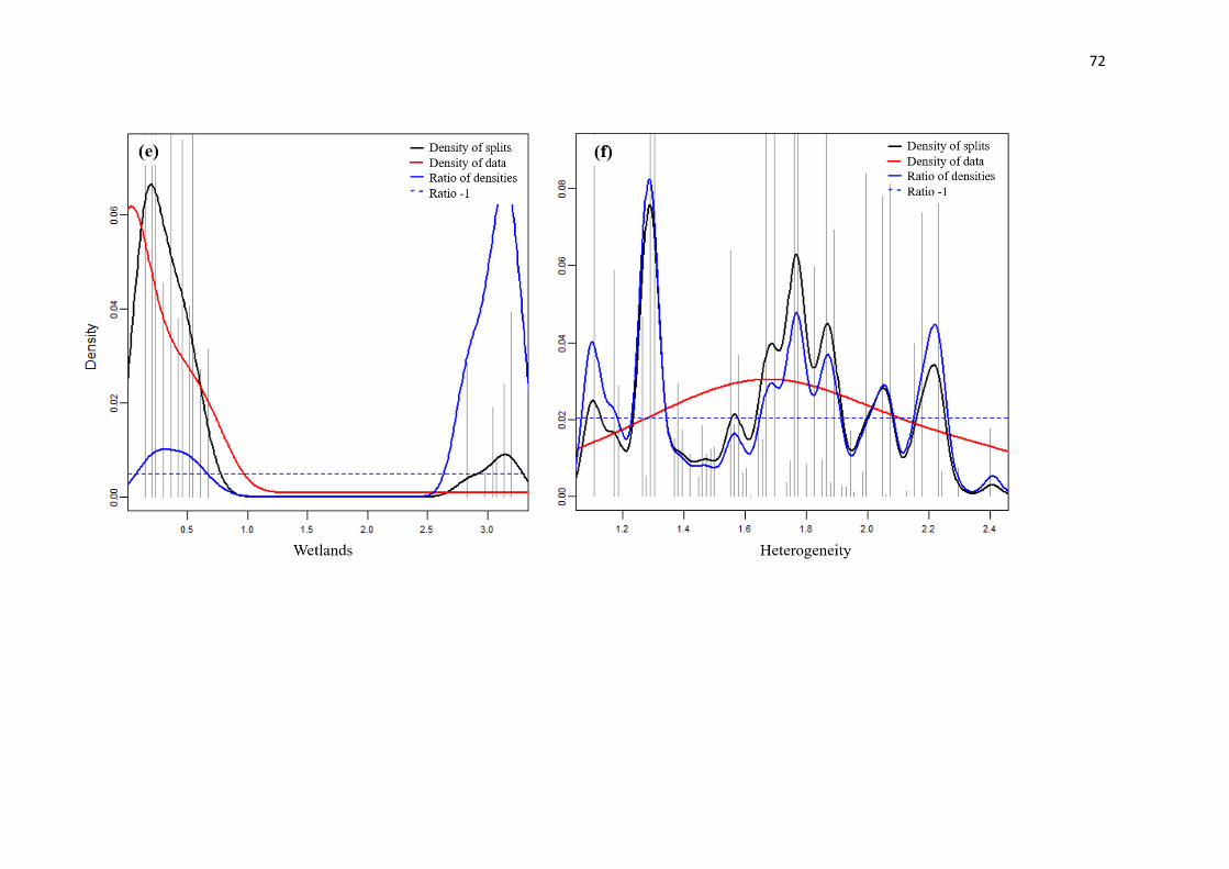
72

73

74

75
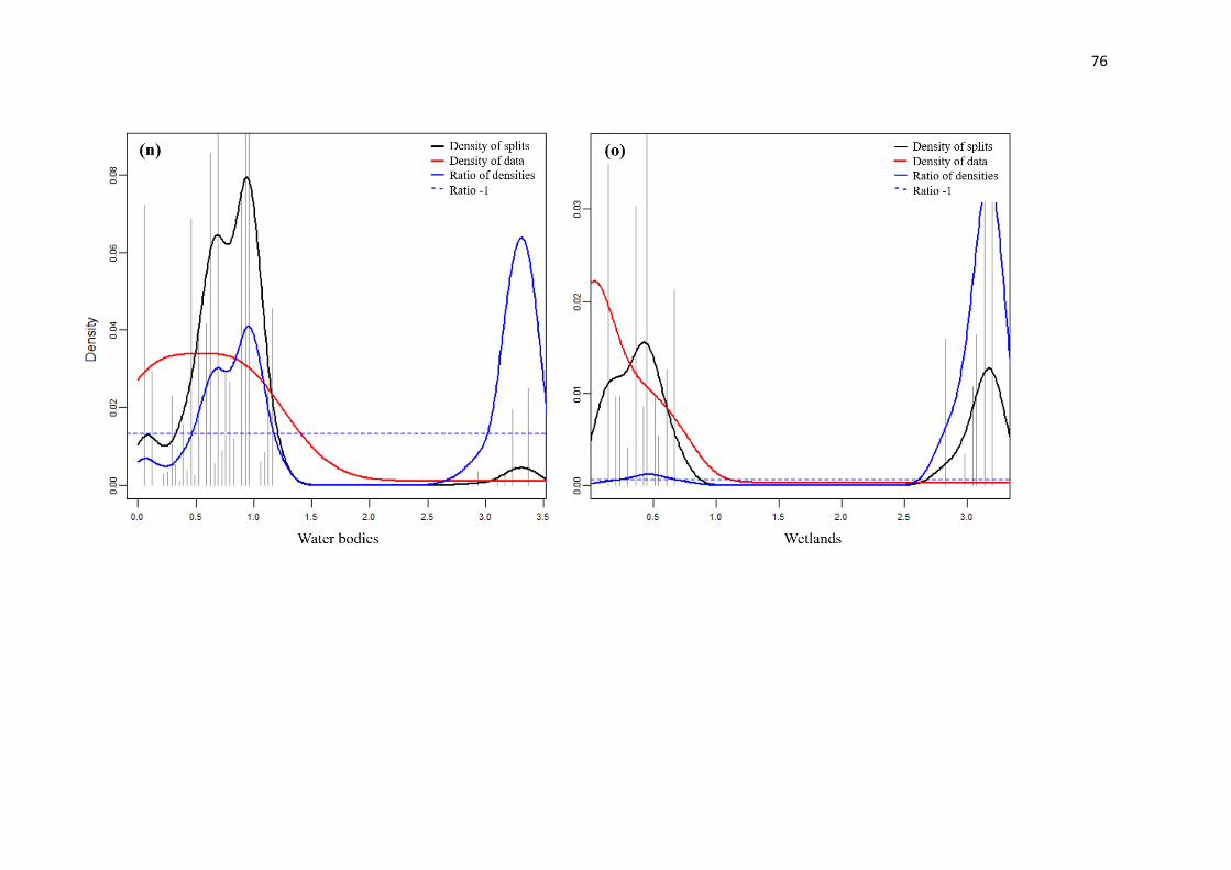
76

77

78
Fig. S33 - Species cumulative plots showing cumulative change in occurrence of individual species/functional response trait/functional response group, where
in the gradient changes occur and which species are most responsible for these changes on each gradient. (a), (b), (c), (d), (e), (f) e (g) are the environmental
gradients to SP. (h), (i) e (j) are the environmental gradients to FRT. (l), (m), (n), (o) e (p) are the environmental gradients to FRG.

79

80

81

82

83

84

85

86

87
ARTIGO 3 - Functional and taxonomic amphibian decline due to
climate change within Brazilian Atlantic Forest
Format based on the guidelines of “Diversity and Distributions”

88
Functional and taxonomic amphibian decline due to climate change within Brazilian
Atlantic Forest
Paula Ribeiro Anunciação1,2,*, Felipe Martello3, Maurício Humberto Vancine2, Raffael Ernst4,
Luiz Marcelo Tavares Carvalho1, Milton Cezar Ribeiro2
1Biology Department, UFLA – Universidade Federal de Lavras, 37200-000, Lavras, Minas Gerais,
Brazil
2São Paulo State University (UNESP), Institute of Biosciences, Department of Ecology, Spatial
Ecology and Conservation Lab (LEEC), Rio Claro, SP, Brazil
3Department of Environmental Sciences, UFSCAR - Universidade Federal de São Carlos, P.O. Box
676, 13565-905 São Carlos, São Paulo, Brazil
4Museum of Zoology, Senckenberg Natural History Collections Dresden, Königsbrücker Landstrasse
159, 01109 Dresden, Germany.
* corresponding author: [email protected]
ABSTRACT
Climate changes are one of the key anthropogenic pressures on biodiversity loss. The
amphibians are especially sensitive to temperature and precipitation alterations, therefore these
species have been negatively affected by climate changes. Herein we applied Ecological Niche
Modelling to evaluate the effect of climate changes on taxonomic and functional richness of
amphibians within Atlantic Forest biome. We have also evaluated how forest-dependent and
open habitat specialists can be affected by climate changes. We expect that (1) both taxonomic
and functional amphibian richness will decrease under climate change; (2) functional richness
will be more affected than taxonomic richness; (3) forest species will be more affected than
open habitat specialists under climate change scenarios. To build taxonomic and functional
prediction maps, we used two scenarios of temperature increase (the Representative
Concentration Pathway, RCP 4.5 and 8.5) for two different temporal climatic scenarios (2050
and 2070). The temperature increase will cause loss of amphibian’s species and functional
diversity. However, contrary to our expectation, the negative impact of climate changes is
greater in taxonomic richness than functional. Both categories of habitat specialists will lose
species, but forest species have greater loss probably due to their high habitat structure
requirements. Taxonomic and functional richness give us complementary information about the
warming future scenarios, being advised to evaluate both indexes to reach an efficient decision-

89
making about mitigation measures. We also recommended paying special attention on forest
species, which seems will be more impacted by the climate changes.
KEY WORDS
Anurans – Species declines – Global warming – Functional trait approach – Functional response
traits
4.1 Introduction
We are facing one of the warmest period on Earth, global average temperature has
increased about 0.85 (0.65 to 1.06) °C over the period 1880 to 2012, with this change in the
temperature being attributed to the intensification of greenhouse gas emission (IPCC, 2014).
The expectation is that global temperature will rise by 0.3 to 4.8 °C by the late-21st century,
but different regions will experience different changes, from cooling to warming (Serreze et al.,
2000). In the Neotropical region, the predictions are quite similar: increased temperature and
length of the dry season, reduced soil moisture and larger interannual variation in rainfall
(Hulme; Viner, 1998). Three consequences for the biodiversity are expected worldwide as a
response to climate change: (i) changes in phenology, (ii) shift in geographic distributions; and
(iii) body-size shrinks (Daufresne et al. 2009).
Amphibians present life-history characteristics such as, permeable and exposed skin,
shell-less eggs, complex life cycles, which make them very sensitive to anthropogenic impacts
(Cushman, 2006; Wells, 2007; Hof et al., 2011; Catenazzi, 2015). Because they are also
ectotherms, the impact of climate change, for instance, can be more severe for them than other
animals (see review Parmesan, 2006; Li et al., 2013). Moreover, temperature is a key abiotic
factor influencing these animals, affecting the aquatic larvae stage, like in the time to hit
metamorphosis and growth rates, body size at metamorphosis, mechanisms of gas exchange,
and energy metabolism rates (Ultsch et al., 1999). Increases in temperature and dryness can
reduce amphibian fecundity (Reading, 2007) and adult recruitment (Lowe, 2012). In a recent
meta-analysis the authors showed that amphibians are breeding earlier than other groups, such
as butterflies, birds and trees (Parmesan, 2007). However, alterations in body size and
morphology of amphibians and poleward shifts in distributions in response to climate change
remains with little evidence (Li et al., 2013). Even if climate change has no direct effects on
amphibian declines, or it presents a non-clear effect, oscillations in climate will severely affect
this taxon. Then, it is necessary to find the best approaches, which can clarify the effects of
climate change in the biodiversity. Functional diversity can be key-component to understand

90
the patterns of temperature variations, with some authors suggesting this approach can
potentially predict the impacts more accurately (Higgins; Strauss, 2008, Dengler et al., 2014;
Pelosi et al., 2014).
Functional traits are efficient to compare broad geographic regions, particularly when
we have interest in communities of different taxa (Ernst, 2012; Simberloff; Dayan, 1991).
Moreover, with the functional characteristics is possible to investigate changes in species traits
along environmental gradients (Vilà-Cabrera et al., 2015; Cornwell; Ackerly, 2009). The
interest on functional diversity is rising between ecologist and conservationist (Tsianou;
Kallimanis, 2016). The literature points that this approach can be more efficient to comprehend
ecosystem resilience and functioning when compared with taxonomic-driven analysis, because
functional diversity is linked to these processes more intensely than other components of
diversity (Ribeiro et al., 2017; Trimble; Van Aarde, 2014, Flynn et al. 2009, Ernst, 2006). At
large extents, the assembly processes can be understood through spatial and temporal patterns
of functional diversity (Petchey et al. 2007).
Studies aiming to understand the spatial distribution of functional diversity are still
scarce (Thuiller et al., 2015; Tsianou; Kallimanis, 2015). In general, these studies are mainly
about whether trait can be predictive of range shift capacity face the climate change, however,
spatial distribution of functional diversity rarely has been evaluated (Iverson et al., 2011;
Chessmann, 2011; Estrada, 2016). Besides that, there are few studies focusing on the impact of
climate changes in amphibians of tropical areas at large scale (Li et al., 2013). Previous studies
about the impact of climate changes in the amphibians of the Brazilian Atlantic Forest showed
it will be a decreasing number of species under future scenarios and protected areas would
become less effective to protect this taxon (Loyola et al., 2013; Lemes et al., 2013). Amphibians
had been pointed out as one of the animal groups most negatively affected by climate changes
(Parmesan, 2006; Li et al., 2013; Catenazzi, 2015), then we choose this group to develop the
first study about predicting models of functional diversity distribution. To this end, we applied
ecological niche-based models to assess the effect of climate changes on amphibian
communities in Brazilian Atlantic Forest Biome. We addressed three questions: 1) Is the future
distribution of amphibian richness according to climate changes different from the current
distribution? 2) What is the effect of climate changes on functional and taxonomic richness of
amphibians? 3) What is the effect of climate changes on forest and open area species? We
expect that (1) due to the amphibians sensitivity to external conditions variation, both
taxonomic and functional richness will decrease under climate change; (2) because the
functional approach has shown more sensitive to disturbance impact than traditional indexes
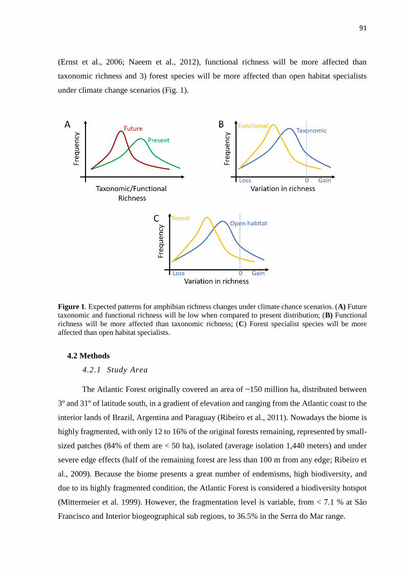
91
(Ernst et al., 2006; Naeem et al., 2012), functional richness will be more affected than
taxonomic richness and 3) forest species will be more affected than open habitat specialists
under climate change scenarios (Fig. 1).
Figure 1. Expected patterns for amphibian richness changes under climate chance scenarios. (A) Future
taxonomic and functional richness will be low when compared to present distribution; (B) Functional
richness will be more affected than taxonomic richness; (C) Forest specialist species will be more
affected than open habitat specialists.
4.2 Methods
4.2.1 Study Area
The Atlantic Forest originally covered an area of ~150 million ha, distributed between
3o and 31o of latitude south, in a gradient of elevation and ranging from the Atlantic coast to the
interior lands of Brazil, Argentina and Paraguay (Ribeiro et al., 2011). Nowadays the biome is
highly fragmented, with only 12 to 16% of the original forests remaining, represented by small-
sized patches (84% of them are < 50 ha), isolated (average isolation 1,440 meters) and under
severe edge effects (half of the remaining forest are less than 100 m from any edge; Ribeiro et
al., 2009). Because the biome presents a great number of endemisms, high biodiversity, and
due to its highly fragmented condition, the Atlantic Forest is considered a biodiversity hotspot
(Mittermeier et al. 1999). However, the fragmentation level is variable, from < 7.1 % at São
Francisco and Interior biogeographical sub regions, to 36.5% in the Serra do Mar range.
92
4.2.2 Ecological Niche Modeling
To predict appropriate current and future areas and thus estimate the change in
taxonomic and functional diversity of amphibians in the Atlantic Forest we used Ecological
Niche Modeling (ENM). ENMs use algorithms to associate occurrences of species to
environmental conditions (generally climatic, such as temperature and precipitation), which
allow us to characterize and delimit the niche of the species (Peterson et al. 2011). We used a
forecast ensemble approach that combines different types of projections, constructed from
various methods and conditions, which results in a more reliable prediction (Araújo and New,
2007, Diniz-Filho et al., 2009).
Presence-only data were obtained from the literature, which used various sources such
as undergrad monographs, dissertations, thesis, articles and books (see supplementary material
for a complete list of references). These data are a subset of ATLANTIC AMPHIBIANS data
paper (Vancine et al., under review) and to our study, this refers more than 240 studies and
about 372 sampling points in the database (Figure 2). The dataset comprises 172 species and
6,657 records. The number of unique records for the species varied from 10 to 230 (average 39
records). More information about these data can be found at
https://github.com/mauriciovancine/ATLANTIC-Amphibians.
We used 19 bioclimatic variables from the WorldClim database at a spatial resolution
of 2.5 minutes (Hijmans et al. 2005). We used the present and future projections of two different
temporal climatic scenarios (2050 and 2070), for two futures warm climate scenarios,
Representative Concentration Pathway (RCP) 4.5 and 8.5. Respectively, these two scenarios
yield warming of 2.3 °C and 4.8 °C. RCP 8.5 is the most pessimistic version to date, with
continuous greenhouse emissions until 2100 producing the most severe global climate change
(Moss et al., 2008). We used the General Circulation Models (GCMs) called ACCESS1-0
developed as collaboration between CSIRO and BoM (Dix et al. 2013).
To avoid collinearity among the variables, we used a factorial analysis with varimax
rotation (”psych” package, R Development Core Team 2017; Revelle, 2017) to reduce the
number of environmental layers. After this step, we selected the five bioclimatic variables that
we consider most relevant to the distribution of tropical amphibians, which are dependent of
warm and rainy weather conditions to breeding: temperature seasonality (Bio4), mean
temperature of the warmest quarter (Bio10), precipitation of wettest month (Bio13),
precipitation seasonality (Bio15), and precipitation of driest quarter (Bio17). For the modeling
of both present and future scenarios, we defined the geographic extent using the Atlantic Forest
93
Domain limit available by Ribeiro et al. (2009), which are available at
https://github.com/LEEClab/ATLANTIC-limits-shapefiles.
We build the ENMs based in four algorithms, the first two are presence-only methods
and the later ones presence-background methods: envelope score – Bioclim (Nix, 1986), Gower
distance method – Domain (Gower distance; Carpenter et al. 1993), other two are machine-
learning methods – Maximum Entropy – MaxEnt (Phillips and Dudík 2008) and Support Vector
Machines (SVM) (Tax and Duin 2004). The ENMs were modeled using “dismo” and “kernlab”
R-packages (Hijmans et al., 2015; Karatzoglou et al., 2004). We modeled each species
individually using a twofold partition approach with 75% train and 25% test. With this
occurrence-partitioned approach, we calculate the evaluation values using True Skill Statistics
(TSS) of each model (Allouche et al. 2006). Through bootstrap analysis, for each algorithm we
randomized each procedure 5 times, resulting in 20 maps (4 algorithms × 5 times) for each
specie. We made the ensemble transforming the 20 continuous maps into binary maps using
“maximum sensitivity and specificity” threshold (Liu et al. 2016). This threshold is
recommended when presence-only data are available in the niche modeling analysis (Liu et al.,
2013, 2016). To predict the final species distribution maps, we overlapped the maps from the
same algorithms and the maps between algorithms. Thus, the final maps have cell values
varying between 0 and 20, which represents the frequency that the model predicted each cell as
suitable of each species. This process was made to present models and used the same thresholds
of present models for future models.

94
Figure 2 - Spatial distribution of amphibian surveys (dark gray dots) into Brazilian Atlantic
Forest. These data represent a subset of ATLANTIC AMPHIBIANS dataset (Vancine et al.,
under review). The boundaries are based on Ribeiro et al. (2009).
4.2.3 Functional response traits selection
We selected seven functional traits to calculate functional diversity inferring about
amphibian characteristics that would be affected by climate changes (Table 1). The
dimorphism, movement index, and mouth area were continuous traits and we measured in male
specimens from Célio F. B. Haddad amphibian collection, housed in the Universidade Estadual
Paulista (UNESP), Rio Claro, SP (CFBH). We measured the traits of anurans species from the
Atlantic Forest which have the minimum number of specimens in biological collections (6 to
20 individuals per species, 129 species) and also have the minimum number of occurrence
points equals to 10. The others four traits, activity, reproductive mode, ecotype and
reproduction habitat, were categorical and the information were taken from literature.
Moreover, the female SVL (snout venter length), which area used to calculate the dimorphism,
was also obtained from the literature (Haddad et al., 2013

95
Table 1. Description of the traits measured or compiled from the literature on amphibian species of the Atlantic Forest Biome.
Functional trait Definition Specific functions Ecosystem process relationship
Dimorphism Male SVL / Female SVL Physiology and ecology characters Related to the energy flow through trophic
chains as predator or prey
Movement index Arm length / leg length Dispersal ability Related to the energy flow through trophic
chains as predator or prey
Mouth area Depth mouth / width mouth Foraging tactics, predator-prey relationships Related to the energy flow through trophic
chains as a predator
Activity Diurnal, nocturnal and both Dispersal ability, predator-prey relationships,
sexual selection
Related to the energy flow through trophic
chains as predator or prey
Reproductive mode 1 to 39 modes Dispersal ability, predator-prey relationships,
sexual selection
Related to the energy flow through trophic
chains as predator or prey
Ecotype
Arboreal, leaf-litter, fossorial, terrestrial,
arboreal+leaf-litter, semi-aquatic,
rheophilic
Dispersal ability, predator-prey relationships Related to nutrient recycling and energy flow
through trophic chains as predator and prey
Reproduction habitat Lentic. Lotic or independent Dispersal ability, predator-prey relationships,
sexual selection
Related to the energy flow through trophic
chains as predator or prey
96
4.2.4 Taxonomic and functional diversity
To calculate taxonomic diversity per each pixel of Atlantic Forest biome, we first
convert all ENMs in binary maps, using the Lowest Presence Threshold (LPT) to classify each
cell, which refers to the lowest frequency that the model predicted the species occurrence
(Pearson et al., 2007). Therefore, we classified cell with values equal or higher than LPT as
“occurs” (value 1) and cell with lower values than LPT as “does not occur” (value 0). To
facilitate the reading of next steps, we consider that “occurs” as presence and “doesn’t occur”
as absence of the species. By summing these classified maps of all species in a determined
scenario, we generated the taxonomic diversity map, wherein the value of each cell represents
the potential richness of these cells.
Then, we calculated functional diversity for each cell of the Atlantic Forest biome. To
this, we first converted the presence-absence maps into community matrixes, wherein each row
represents each cell of the models and columns the species presence or absence (0 or 1 values).
Afterwards, we converted categorical variables in fuzzy variables and in sequence in proportion
variable using the prep.fuzzy variable from the ade4 package (Pavoine 2009). Using all
variables, we generate a traits distance matrix with the dist.ktab function and posteriorly we
combined this matrix with the presence-absence community matrixes to calculate functional
richness (FRic) with the dbFD function from FD package. FRic represents the hypervolume in
the multivariate trait space that each community occupies. Once our interest was to compare
diversity between scenarios, we bind presence-absence community matrixes of all scenarios
before calculating FRic. We have also standardized FRic by “global FRic”, which represents a
community with all species that occurred in all scenarios and have value equal to 1.
After FRic calculation, we separated the cells of each scenario and created a matrix of
FRic, and converted it into a map of functional diversity, wherein the value of each cell
represents the estimated functional diversity.
4.2.5 Analysis
We used Kruskal-Wallis to test the significance of the difference between the present
distribution maps and the prediction maps of the four different scenarios of climate change: two
different temporal climatic scenarios [2050 and 2070] and two futures warm climate scenarios
[RCP4.5 and RCP 8.5]) for each biodiversity level and for the two groups of habitat specialist
species. For each biodiversity level (taxonomic and functional richness), we made the

97
subtraction of the future prediction maps and present distribution maps and after that, tested
whether the difference is equal to zero with one sample Wilcoxon Signed Rank test. We
performed all that tests in the software R, version 3.0.1 (R development core team, 2014). On
the above analysis, we used every Atlantic Forest pixel.
4.3 Results
4.3.1 Influence of climate changes on taxonomic and functional richness
The comparison of the present and future predictive maps for both taxonomic and
functional richness revealed that Brazilian Atlantic forest localized in the interior areas will lose
species and functions. The loss of species is greater than functions. This is true for all scenarios;
however we highlight the present and the most pessimistic scenarios from both components of
biodiversity in the Figure 3.
The taxonomic richness shows more species with a narrow distribution than functional
richness. In addition, the increasing of temperature will gradually cause a decrease in the
distribution range of the amphibian species and functional response traits or in other words, the
scenarios of species and functions lost will get worse according the gradual increase of
temperature (Fig. 4). According the most pessimist scenario, there is a peak of narrow
distribution species in both components (Fig. 4). The two components of biodiversity show a
positive correlation; however it is not a complete overlap, which indicate complementary
information (Fig. S41 – Supplementary material 3). In all future predictions, the range of
species distribution will decrease extensively (to both biodiversity levels), as great part of
richness difference distributions are negative (Fig. 5).
4.3.2 Influence of climate changes according to habitat specialization
With the temperature increase, both categories of habitat specialist species show loss of
species with bigger distribution range. However, forest species presents a narrower distribution
than open area species. Except for the most pessimistic scenarios that show very similar pattern
between the two categories of species. Even open area species keeping the bigger range of
distribution, both categories will have a decrease in the number of species with big range of
distribution (Fig. 5).

98
Figure 3. Taxonomic richness (left panels) and functional richness (right panels) for Atlantic
Forest amphibians for the present (top panels) and for the year 2070 (bottom panels) according
the most pessimistic scenarios of temperature increase. A. Taxonomic richness of present. B.
Functional richness of present. C. Taxonomic richness of 2070’s. D. Functional richness of
2070’s.

99
Figure 4. Functional and taxonomic richness frequency of Atlantic Forest amphibians
according two scenarios of temperature increase (RCP 4.5 and RCP 8.5) and to the years of
2050 and 2070. In gray we represent the present estimates. Fric = fuctional richness; Richness
= taxonomic richness.

100
Figure 5. Difference between the future and present functional and taxonomic richness of
Atlantic Forest amphibians, according two scenarios of temperature increase (RCP 4.5 and RCP
8.5) and two years (2050 and 2070). FRic = functional richness; richness = taxonomic richness.
Dashed gray line represents zero of difference.

101
Figure 5. Taxonomic richness frequency of Atlantic Forest amphibians according two
scenarios of temperature increase (RCP 4.5 and RCP 8.5) and to the years of 2050 and 2070 for
the forest species specialists (left panels) and open area specialists (right panels).
4.4 Discussion
Climate change will cause severe species loss, compromising species with particular
traits, and functional richness will be restricted mainly to regions next to the coast. Moreover,
the loss of species seems to be worse, with taxonomic richness being affected more than the
functional one. When comparing taxonomic and functional biodiversity components under

102
climate chance we observe that they present complementary information and can offer relevant
insights about amphibian conservation. As we expected, species dependent of forest habitats
are more sensitive than open-area species and their distribution range will shrink (see also
Keinath et al., 2017).
4.4.1 Climate changes influence both taxonomic and functional richness
The Brazilian Atlantic forest is losing species faster than functional response traits.
Functional richness will be bigger in the future than taxonomic richness, mainly in the northeast.
This result indicates the lost species share similar traits or in other words, we are losing
functionally redundant species. The climate changes are filtering out these species with traits
that are poorly adapted to the new conditions and permitting colonization by better-adapted
species (Mouillot et al., 2013). Even though the two components of biodiversity are not totally
correlated, the relationship is positive. Diaz and Cabido (2001) propose this can happen when
species converge into relatively discrete functional strategies. However, competition can mask
the disturbance impact on the functional structure of communities favoring the coexistence of
dissimilar combinations of traits (MacArthur and Levins, 1967; Schamp and Aarssen, 2009).
This set of dissimilar traits means lack of functional redundancy, which may disturb the
ecosystem process and reduce ecosystem resilience (Davic and Welsh 2004). A future without
functionally redundant species can have a huge impact on the ecosystem process, because each
species extinction will decrease the functional diversity. Then, the climate changes impact can
be even worse than we are seeing in the predictive maps.
Trait-based measures are better predictors of disturbance impact and ecosystem process
(Ernst et al., 2006; Naeem et al., 2012; Mouillot et al., 2013), being capable to detect changes
in biodiversity due anthropogenic disturbances before extinctions effectively occur (Mouillot
et al., 2013). In our study, taxonomic richness shows a pattern of potential lost more evident.
This can indicate two responses, or taxonomic richness is more sensitive to climate changes
than functional trait approach or the future is not so pessimist how we expected. However,
because amphibians are a very sensitive group to temperature and precipitation (Duellman and
Trueb, 1994), probably the first option is the correct. Moreover, the correlation between
taxonomic and functional richness were found in many studies (Mayfield et al. 2010; Riemann
et al., 2017), but the exact relationship between these two components of biodiversity is not
clear for the majority of natural systems (Naeem, 2002). In our case, there is not a complete
overlapping of the components of biodiversity responses, what makes advised to consider both
when takes conservation measures.

103
A big part of the remaining taxonomic and functional richness of Atlantic Forest
Hotspot will be restricted to southeast region close to the coast. This will be a conservation
challenge, because this area has a huge property speculation (Dean, 1996), moreover, it is the
most developed region of the country. Other studies in the same biome, but evaluating
amphibians’ richness presented a similar pattern of species loss (Lemes et al., 2013; Loyola et
al., 2013). Due to the lack of latitudinal temperature gradient of the lowland regions in the
tropics, range shifts probably would happen in higher elevations, such as in southeast of Brazil
(Colwell et al. 2008; Carnaval et al., 2009; Lemes et al., 2013). The southeast region, where the
main amphibians richness would be concentrated, is a mountainous region and major areas of
endemism, acting as important refuges for species under climate changes (Araújo et al., 2011;
Klorvuttimontara et al. 2011).
4.4.2 Forest dependent are more affected than open habitat species
Climate changes acting as an environmental filter can often favor generalist species
(Ribeiro et al., 2017) such as open area habitat species. The latter species usually have large
ranges of distribution and tolerate an extensive diversity of conditions, while small range
species to persist require a set of specific conditions (Cooper et al. 2008; Devictor et al. 2010).
In our study, we found exactly this pattern, showing the changes in climate will be affect
stronger the forest associated species, which are the most sensitive species related to open area
species. In addition, we can notice that the response to disturbance is not identical to the species,
rejecting the neutral model and giving support for a niche model (Mouillot et al., 2013). The
niche processes driving community responses to disturbance can allow prediction of impacts in
the structure of functional trait, therefore the functioning of communities (Pakeman, 2011).
Then, knowing the increase of temperature will be worse to forest species, we should
concentration efforts in this group to avoid lose important functional traits.
The impact of climate changes in species, especially the more sensitive such as forest-
dependents, probably will be aggravated by habitat loss and fragmentation. Even though, we
have not considered the landscape pattern in our models, the impact of habitat fragmentation
and loss is well established, recognized as the major threats to biodiversity (Newbold et al.,
2014). The increase of CO2 concentration can lead to an agriculture production intensification,
which can generate a larger demand for farming areas (Van Ierland et al., 2001). Besides the
agricultural development, landscapes with main anthropogenic land use will continue to change
due to increasing urbanization and economic mobility (Opdam and Wascher, 2004). All these
factors will contribute to habitat fragmentation and loss, which in synergy with climate changes
104
will decrease the adequate habitat for biodiversity. However, the only study indicating this
synergy was developed by Warren et al. (2001), who found that in severely fragmented
landscapes there is no range expansion of a British butterfly. Clearly, species associated with
forest areas and low dispersal abilities will be the most impacted, also fragmentation seems to
increase the climate change impact on biodiversity (Opdam and Wascher, 2004).
4.5 Management recommendations
In order to have a more accurate prediction of the climate changes impact, we
recommended to investigate what kind of trait is being filtered out by the climate changes. This
kind of response will indicate what functional trait is related to this anthropogenic disturbance,
in addition reveal which species are more sensitive. Another important approach is to include
in the prediction models the landscape pattern to help understand the synergistic effects and
reveal what is the role of land cover changes in the biodiversity loss and ecosystem functioning.
Moreover, extra studies investigating the role of temperature increase in functional diversity,
mainly in tropical areas, are necessary.
This study is the first one to evaluate the effects of climate changes on functional traits
of a vertebrate group. We showed that amphibian taxonomic and functional richness are
complementary indexes being advised to analyze both responses before taking conclusions.
Conservation efforts should be localized in the southeast region of Brazil, which represents an
important refuge to amphibians. In addition, special attention on forest associate species is
advised. Ecological niche models can offer an important prognosis about species distribution
in the future, according anthropogenic disturbances, being a valuable tool to take decisions in
conservation and ecosystem management (Wittmann et al., 2016). However, this kind of
modeling often only considerate climate variables and species presence data, species functional
traits are rarely incorporate in the modeling steps restricting our understanding of the impact
and power of decision.
REFERENCES
Allouche, O., Tsoar, A., & Kadmon, R. (2006) Assessing the accuracy of species distribution
models: prevalence, kappa and the true skill statistic (TSS). Journal of Applied Ecology, 43,
1223–1232, http://dx.doi.org/10.1111/j.1365-2664.2006.01214.x.
Araújo, M.B., & New, M. (2007). Ensemble forecasting of species distributions. Trends in Ecology
and Evolution, 22, 42 – 47.
Carpenter, G., Gillison, A. N. & Winter, J. (1993). DOMAIN: a flexible modelling procedure for
mapping potential distributions of plants and animals. Biodiversity and Conservation, 2, 667–
680, http://dx.doi.org/10.1007/BF00051966.

105
Chessman, B. C. (2012). Biological traits predict shifts in geographical ranges of freshwater
invertebrates during climatic warming and drying. Journal of Biogeography, 39, 957–969.
Cornwell, W. K. & Ackerly, D.D. (2009). Community assembly and shifts in the distribution of
functional trait values across an environmental gradient in coastal California. Ecological
Monographs, 79, 109–126.
Cooper, N., Bielby, J., Thomas, G.H., & Purvis, A. (2008). Macroecology and extinction risk
correlates of frogs. Global Ecology and Biogeography, 17, 211–221.
Devictor, V., Mouillot, D., Meynard, C., Jiguet, F., Thuiller, W., & Mouquet, N. (2010). Spatial
mismatch and congruence between taxonomic, phylogenetic and functional diversity: the need
for integrative conservation strategies in a changing world. Ecology Letters, 13, 1030–1040
Daufresne, M., Lengfellner, K., & Sommer, U. (2009). Global warming benefits the small in aquatic
ecosystems. PNAS, 106, 12788–93.
Davic, R. D., & Welsh, H. H. (2004). On the ecological roles of salamanders. Annual Review of
Ecology, Evolution and Systematics, 35:405–434
DEAN, W. (1996) A ferro e fogo: a história e a devastação da Mata Atlântica brasileira. São Paulo:
Companhia das Letras.
Dengler, J., Janišová, M., Török, P., & Wellstein, C. (2014). Biodiversity of palaearctic grasslands:
a synthesis. Agriculture, Ecosystems & Environment, 182, 1-14.
http://dx.doi.org/10.1016/j.agee.2013.12.015.
Diaz, S., & Cabido, M. (2001) Vive la difference: plant functional diversity matters to ecosystem
processes. Trends in Ecology & Evolution, 16, 646–655.
Diniz-Filho, J. A., Bini, L. M., Rangel, T. F., Loyola, R. D., Hof, C., Nogués- Bravo, D., & Araújo,
M. B. (2009) Partitioning and mapping uncertainties in ensembles of forecasts of species
turnover under climate change. Ecography, 32, 897–906.
Dix, M., Vohralik, P., Bi, D., Rashid, H., Marsland, S., O'Farrell, S., Uotila, P., Hirst, T.,
Kowalczyk, E., Sullivan, A., Yan, H., Franklin, C., Sun, Z., Watterson, I., Collier, M., Noonan,
J., Rotstayn, L., Stevens, L., Uhe, P. and Puri, K., The ACCESS couple model: documentation
of core CMIP5 simulations and initial results, Australian Meteorological and Oceanographic
Journal, 63, 83-99, 2013.
Duellman, W. E., & Trueb, L. (1994). Biology of Amphibians. Baltimore: The Johns Hopkins
University Press.
Ernst, R., Linsenmair, K.E., & Rodel, M.O. (2006). Diversity erosion beyond the species level:
dramatic loss of functional diversity after selective logging in two tropical amphibian
communities. Biological Conservation, 133, 2, 143-155.

106
Ernst R., Keller A., Landburg G., Grafe T. U., Linsenmair K. E., Rödel M. O., & Dziock F. (2012).
Common ancestry or environmental trait filters: Cross‐continental comparisons of trait–habitat
relationships in tropical anuran amphibian assemblages. Global Ecology and Biogeography, 21,
704–715.
Estrada, A., Morales-Castilla, I., Caplat, P., & Early, R. (2016). Usefulness of Species Traits in
Predicting Range Shifts. Trends in Ecology & Evolution, 31, 190 – 203.
Flynn D. F. B., Gogol-Prokurat M., Nogeire T., Molinari N., Richers B. T., Lin B. B., Simpson N.,
Mayfield, M. M., & DeClerck F. (2009) Loss of functional diversity under land use
intensification across multiple taxa. Ecological Letters, 12, 22–33.
Haddad, C. B. F. et al. (2013). Guia dos Anfíbios da Mata Atlântica: Diversidade e Biologia. São
Paulo: Anolis Books Editora.
Higgins, C. L. & Strauss, R. E. (2008). Modeling Stream Fish Assemblages with Niche
Apportionment Models: Patterns, Processes, and Scale Dependence. Transactions of the
American Fisheries Society, 137(3), 696-706.
Hijmans, R. J. et al. (2005). Very high resolution interpolated climate surfaces for global land areas.
International Journal of Climatology, 25, 1965-1978.
Hijmans, R. J., Phillips, S. J., Leathwick, J. R., & Elith, J. (2015). Dismo: SpeciesDistribution
Modeling. R package version 1.0-12.
Hijmans, R.J. & van Etten, J. (2012). raster: Geographic analysis and modeling with raster data. R
package version 2.0-12. http://CRAN.R-project.org/package=raster
Hulme, M. & Viner, D. (1998). A climate change scenario for the tropics. Climatic Change, 39,
145–176.
IPCC. (2014). Climate Change 2014: Synthesis Report. Contribution of Working Groups I, II and
III to the Fifth Assessment Report of the Intergovernmental Panel on Climate Change [Core
Writing Team, R.K. Pachauri and L.A. Meyer (eds.)]. IPCC, Geneva, Switzerland, 151 pp.
Iverson, L., Prasad, A. M., Matthews, S., & Peters, M. (2011). Lessons learned while integrating
habitat, dispersal, disturbance, and life-history traits into species habitat models under climate
change. Ecosystems, 14, 1005–1020.
Karatzoglou, A., Smola, A., Hornik, K., & Zeileis, A. (2004). kernlab – an S4 Package for Kernel
Methods in R. J. Stat. Softw. 11, 1–20,http://dx.doi.org/10.1016/j.csda.2009.09.023.
Keinath, D. A., Doak, D.F., Hodges, K.E., Prugh, L.R., Fagan, W., Sekercioglu, C.H., Buchart, S.
H. M., Kauffman, & Source, M. (2017) A global analysis of traits predicting species sensitivity
to habitat fragmentation. Global Ecology and Biogeography, 26(1), 115-127.
Laliberté, E., Legendre, P., & B. Shipley. (2014). FD: measuring functional diversity from multiple
traits, and other tools for functional ecology. R package version 1.0-12.

107
Li, Y., Cohen, J.M., & Rohr, J.R. (2013). A review and synthesis of the effects of climate change
on amphibians. Integrative Zoology, 8, 145-161
Liu, C., White, M., & Newell, G. (2013) Selecting thresholds for the prediction of species
occurrence with presence-only data. Journal of Biogeography, 40, 778–789.
http://dx.doi.org/10.1111/jbi.12058.
Liu, C., Newell, G., & White, M. (2016). On the selection of thresholds for predicting species
occurrence with presence-only data. Ecology and Evolution, 6, 337–348,
http://dx.doi.org/10.1002/ece3.1878.
Lowe, W. H. (2012). Climate change is linked to long-term decline in a stream salamander.
Biological Conservation, 145, 48–53.
MacArthur, R. & Levins, R. (1967) Limiting similarity convergence and divergence of coexisting
species. American Naturalist, 101, 377–387.
Mayfield, M. M., Bonser, S. P., Morgan, J. W., Aubin, I., McNamara, S.&Vesk, P.A. (2010) What
does species richness tell us about functional trait diversity? Predictions and evidence for
responses of species and functional trait diversity to land-use change. Global Ecology and
Biogeography, 19, 423–431.
Mittermeier, R. A., Myers, N., Robles Gil, P., & Mittermeier, C.C. (1999). Hotspots. Agrupación
Sierra Madre, CEMEX, Mexico City.
Moss, R., et al. (2008). Towards New Scenarios for Analysis of Emissions, Climate Change,
Impacts, and Response Strategies. Intergovernmental Panel on Climate Change, Geneva,
Switzerland. 25 pp.
Mouillot, D., et al. (2013). A functional approach reveals community responses to disturbances.
Trends in Ecology & Evolution, 28(3), 167–177.
Naeem, S. (2002). Disentangling the impacts of diversity on ecosystem functioning in combinatorial
experiments. Ecology, 83, 2925–2935.
Naeem, S. et al. (2012). The functions of biological diversity in an age of extinction. Science, 336,
1401–1406.
Newbold, T., Hudson, L. N., Phillips, H. R .P., Hill, S. L. L., Contu, S., Lysenko, I., Blandon, A.,
Butchart, S. H. M., Booth, H. L., Day, J., De Palma, A., Harrison, M. L. K., Kirkpatrick, L.,
Pynegar, E., Robinson, A., Simpson, J., Mace, G. M., Scharlemann, J. P. W. & Purvis, A. (2014).
A global model of the response of tropical and sub-tropical forest biodiversity to anthropogenic
pressures. Proceedings of the Royal Society of London Series B, Biological Sciences, 281,
20141371

108
Nix, H. (1986). A biogeographic analysis of Australian elapid snakes. In: Longmore,R. (Ed.), Atlas
of Elapid Snakes of Australia. Australian Government Publishing Service, Canberra, Australia,
pp. 4–15.
Oksanen, J., Kindt, R., Legendre, P., O’Hara, B., Simpson, G. L, Solymos, P., Stevens, M. H. H.,
& Wagner, H. (2008) Vegan: Community Ecology Package. R package version 1.15-0.
http://cran. r-project.org/, http://vegan.r-forge.r-project.org/
Opdam, P., & Wascher, D. (2004). Climate change meets habitat fragmentation: linking landscape
and biogeographical scale levels in research and conservation. Biological Conservation, 117,
285–297
Pakeman, R. J. (2011) Multivariate identification of plant functional response and effect traits in an
agricultural landscape. Ecology, 92, 1353–1365.
Parmesan, C. (2006). Ecological and Evolutionary Responses to Recent Climate Change. Annual
Review of Ecology, Evolution and Systematics, 37, 637-669.
doi:10.1146/annurev.ecolsys.37.091305.110100
Parmesan, C. (2007) Influences of species, latitudes and methodologies on estimates of
phenological response to global warming. Global Change Biology, 13, 1860–72.
Pearson, R. G., Raxworthy, C. J., Nakamura, M., & Townsend Peterson, A. (2007). Predicting
species distributions from small numbers of occurrence records: a test case using cryptic geckos
in Madagascar. Journal of biogeography, 34(1), 102-117.
Pelosi, C., Pey, B., Hedde, M., Caro, G., Capowiez, Y., Guernion, M., Peigné, J., Piron, D.,
Bertrand, M. & Cluzeau, D. (2014) Reducing tillage in cultivated fields increases earthworm
functional diversity. Applied Soil Ecology, 83, 79-87.
http://dx.doi.org/10.1016/j.apsoil.2013.10.005.
Petchey, O. L., Evans, K. L., Fishburn, I.S., & Gaston, K. J. (2007). Low functional diversity and
no redundancy in British avian assemblages. Journal of Animal Ecology, 76, 977–985.
Peterson, A. T., Soberón, J., Pearson, R. G., Anderson, R. P., Martínez-Meyer, E., Nakamura, M.,
& Araújo, M. B. (2011). Ecological niches and geographic distributions. Monographs in
population biology 49. Princeton, NJ: Princeton University Press.
Phillips, S. J., & Dudík, M. (2008). Modeling of species distributions with Maxent: newextensions
and a comprehensive evaluation. Ecography (Cop.), 31, 161–
175,http://dx.doi.org/10.1111/j.2007.0906-7590.05203.x.
R development core team. R: A language and environment for statistical computing. 2014. R
Foundation for Statistical Computing, Vienna, Austria. Disponível em: <http://www.R-
project.org/.>. Acesso em: 07 aug. 2015.

109
Reading, C. (2007) Linking global warming to amphibian declines through its effects on female
body condition and survivorship. Oecologia, 151, 125–31.
Revelle, W. (2017) psych: Procedures for Personality and Psychological Research, Northwestern
University, Evanston, Illinois, USA, https://CRAN.R-project.org/package=psych Version =
1.7.8.
Ribeiro, M. C. et al. (2009) The Brazilian Atlantic Forest: how much is left, and how is the
remaining forest distributed? Implications for conservation. Biological Conservation, 142: 1141-
1153.
Ribeiro, J., Ferreira, E., Batista, R., Soares, A., Colli, G. R. & Caldwell, J.P. (2017). Evidence of
neotropical anuran community disruption on rice crops: a multidimensional evaluation.
Biodiversity and Conservation, 26, 3363-3383.
Riemann J. C., Ndriantsoa S. H., Rödel M. O. & Glos, J. (2017). Functional diversity in a
fragmented landscape — Habitat alterations affect functional trait composition of frog
assemblages in Madagascar. Global Ecology and Conservation, 10, 173-183.
Schamp, B. S. & Aarssen, L.W. (2009). The assembly of forest communities according to maximum
species height along resource and disturbance gradients. Oikos, 118, 564–572.
Serreze, M. C., Walsh, J. E., Chapin,F. S., Osterkamp, T., Dyurgerov, M., Romovsky, V., Oechel,
W. C., Morison, J., Zhang, T. & Barry, R.G. (2000). Observational evidence of recent change in
the northern high-latitude environment. Climatic Change, 46, 159–207.
Simberloff, D., & T. Dayan. (1991). The guild concept and the structure of ecological communities.
Annual Review of Ecology and Systematics, 22,115–143.
Tax, D. M. J., & Duin, R. P. W. (2004). Support vector data description. Machine Learning, 54,
45–66, http://dx.doi.org/10.1023/B:MACH.0000008084.60811.49.
Trimble, M. J., & Van Aarde, R. J. (2015). Amphibian and reptile communities and functional
groups over a land-use gradient in a coastal tropical forest landscape of high richness and
endemicity. Animal Conservation, 175, 441-453.
Thuiller, W., Lavorel, S., Sykes, M. T. & Araújo, M. B. (2006). Using niche-based modelling to
assess the impact of climate change on tree functional diversity in Europe. Diversity and
Distributions, 12, 49–60.
Tsianou, M. A. & Kallimanis, A. S. (2016). Different species traits produce diverse spatial
functional diversity patterns of amphibians. Biodiversity and Conservation, 25, 117–132,
10.1007/s10531-015-1038-x.
Ultsch, G. R., Bradford, D. F. & Freda, J., (1999) Physiology: coping with the environment. In:
Tadpoles: the biology of anuran larvae: 189–214 (R. W. McDiarmid and R. Altig, Eds.). Univ.
of Chicago Press, Chicago.
110
Vancine, M. H., K. S. Duarte, Y. S. Souza, J. G. R. Giovanelli, P. M. M. Sobrinho, A. López, R. P.
Bovo, F. Maffei, M. B. Lion, J. W. Ribeiro-Júnior, R. Brassaloti, C. Ortiz, H. O. Sawakuchi, J.
Bertoluci, L. R. Forti, P. Cacciali, C. F. B. Haddad, and M. C. Ribeiro. ATLANTIC
AMPHIBIANS. A Dataset of Amphibian Communities from the Atlantic Forests of South
America. Ecology (under review).
Van Ierland, E. C., De Groot, R. S., Kuikman, P. J., Martens, P., Amelung, B., Daan, N., Huynen,
M., Kramer, K., Szonyi, J., Veraart, J. A., Verhagen, A., van Vliet, P. E. V., & Westein, E.
(2001). Integrated Assessment of Vulnerability to Climate Change and Adaptation Options in
the Netherlands. Wageningen University and Research Centre, Wageningen, report No 952274.
Vilà-Cabrera, A., Martínez-Vilalta, J. & Retana, J. (2015), Functional trait variation along
environmental gradients in temperate and Mediterranean trees. Global Ecology and
Biogeography, 24, 1377–1389. doi:10.1111/geb.12379.
Warren, M. S., Hill, J. K., Thomas, J .A., Asher, J. A., Fox, R., Huntley, B., Roy, D .B., Teffer, M.
G., Jeffcoate, S., Harding, P., Jeffcoate, G., Willis, S. G., Greatorex-Davies, J. N., Moss, D., &
Thomas, C.D. (2001). Rapid responses of British butterflies to opposing forces of climate and
habitat change. Nature, 414, 65–69.
Wittmann, M. E., Barnes, M. A., Jerde, C. L., Jones, L. A., & Lodge, D. M. (2016). Confronting
species distribution model predictions with species functional traits. Ecology and Evolution, 6,
873-879(7).

111
Supplementary material 3
Fig. S41. Scatter-plot showing the relationship between functional richness and taxonomic
richness of Atlantic Forest amphibians for the present and for the two scenarios of temperature
increase, RCP 4.5 (prediction of 2.3ºC temperature increase) and RCP 8.5 (prediction of 4.9ºC
temperature increase) for the years of 2050 and 2070. Frich = functional richness; Richness =
taxonomic richness.

112
CONCLUSION
In this thesis, I aimed to understand the effects of anthropogenic disturbances on
amphibians’ communities across highly fragmented and threatened forest ecosystem. I used
data about amphibians’ communities sampled through a new tool called “Automated Recording
Systems”. This allow simultaneous, long-time and permanent sampling of vocalizing animals,
besides cross-validation of the data by experts. In addition, I used auditory and visual surveys
of amphibians to supplement the passive acoustic monitoring and avoid locality bias. At
landscape level across a habitat loss and fragmentation gradient, I found that anthropogenic
environmental gradients, created by suppression of native habitat and establishment of different
land uses, cause turnover of amphibians’ species, functional response traits and functional
response groups. In a large scale level –Atlantic Forest hotspot – I found that temperature
increase will causes taxonomic amphibians’ species decline, but this decline is will be smaller
for functional diversity amphibians. My findings indicate that trait-approach is complementary
to classical measures of diversity, such as taxonomic richness, to elucidate the effects of human-
induced changes on biodiversity. Therefore, the combination of these approaches guarantees
better understanding of anthropogenic impacts on amphibian communities. The summary of
each chapter is presented below.
In the first chapter, I aimed to answer the question “how much sampling time is
sufficient to represent amphibian diversity”. Automated recording system generate huge
amount of the data, and the needed time for characterize the species richness at landscape levels
is unknow for many taxa worldwide. In this chapter, I aimed to propose a less time-demanding
to identify amphibians, but with an accurate representation of the community. Using
accumulation curves, I found that 770 minutes are a suitable amount of time to record and listen
to determine the species presence. I have also evaluated if forest amount (%) influences the
needed time to reach richness asymptote on a sampling effort-richness curve. I observed no
correlation between needed time and forest amount; therefore I suggest that the amount of
minutes be a minimum of 770, independent of habitat loss level. Future studies may evaluate
the influence of weather and other environmental covariates in the sound recordings. Besides
that, the development of improved automatic detection algorithms can decrease the time spent
by experts to filter the recordings, as well as helping to provide more reliable data, without
human bias.
In the second chapter, my aim was to identify the best environmental predictors of three
components of diversity (species, functional response traits and functional response groups)

113
and evaluate where important turnover of species/functional traits/functional groups or
ecological thresholds are happening along the anthropogenic environmental gradients. I have
also assessed concordant/non-concordant diversity patterns at the taxonomic and functional level. I
found that silviculture (eucalyptus monoculture), water bodies and environmental heterogeneity
are the main predictors for all components of biodiversity. Moreover, when the interest is
explaining taxonomic composition we need more predictors to explain the variance, than we
need to explain functional components (functional diversity and traits). Indicating that when
the conservation goal is based in the information provide by functional groups or traits, fewer
main parameters are required to be controlled, but if the aim is to safeguard overall taxonomic
diversity, then additional factors may be important. Regarding to the thresholds, eucalyptus and
water bodies amounts showed rapid change in the community already in the beginning of the
gradient. Higher the amount of these variables in the landscape, With the changes, occurred
establishment of traits associated with generalist species. Consequently, the substitution of
suitable habitat by anthropogenic land uses causes disturb on the biodiversity, even though their
proportion in the landscape is not high. However, the main threshold of environmental
heterogeneity is in the middle of the gradient, indicating that until certain point the combination
of natural and anthropogenic areas is beneficial to amphibians, offering complementary
resources. The best management measure to amphibians seems to be the conservation of natural
habitats such as forest in agricultural landscapes, avoiding predominance of certain type of land
uses. Regarding to the responses of the three components of biodiversity, the similarity
indicates the environmental filters constrain functional and taxonomic components in a related
way. The selection of what component of biodiversity to use for making decisions depends on
the conservation goal. If the objective is to protect the whole community, probably it is not
necessary the analysis of other levels of biodiversity, only the classic descriptors of biodiversity
– such as species diversity, species richness and total abundance - seem to be enough.
Nonetheless, when emblematic, sensitive species are the priorities and when the proposal is to
keep the functional integrity, we recommended exploring functional traits and related indexes.
In the last chapter, I investigated the influence of climate changes on taxonomic and
functional richness of amphibians. Even though recent studies demonstrated functional
diversity as a more efficient biodiversity measure for understanding the response of biodiversity
to anthropogenic disturbance, with the temperature increase the loss of species is greater than
loss of functions. This can happen because the climate changes will exclude species functionally
redundant what results in a pattern loss more prominent in taxonomic richness. Despite this
difference between the two components of diversity (taxonomic vs functional), a large portion

114
of the remaining taxonomic and functional richness will be concentrate on southeast region of
the Atlantic Forest hotspot, particularly close to coastal areas. It will be challenging to the
conservation measures, because it is a region that encompass the highest population density in
the biome, subject to urban expansion. The two components of diversity showed
complementary responses, therefore both taxonomic and functional richness need to be
considered when defining conservation strategies for biodiversity conservation and related
ecosystem services provision. In addition, the impact of temperature increase will be worse on
forest specialist species, probably because this habitat specialist group has higher requirements
of habitat structure. Climate changes in synergy with habitat loss and fragmentation probably
will be the drivers of the more intense impact on forest species. However, both habitat specialist
groups show species loss. We recommend studies evaluating which traits the climate changes
are filtering out and to incorporate the landscape pattern. Moreover, more studies about the role
of temperature increase in functional diversity are indicated to obtain a clearer response of the
impact and guide mitigation measures.
The human-induced changes have negative impact on biodiversity in the present and
will continues in the future. Therefore, whether mitigation and conservation measures need to
be taken in order to safeguard both species diversity, functional diversity and consequently their
ecosystem services and functions. Habitat loss and fragmentation, substitution of native habits
by anthropogenic land uses, in synergism with negative climate changes effects, are altering
amphibians’ community composition leading to predominance of less sensitive and impact-
tolerant species. This can have a huge impact on ecosystems functioning because important
functions are being lost. Functional component is effective to evaluate and to predict the impact
on biodiversity and should be considered as a complementary approach to classical diversity
measures.