land matters. an impact evaluation in developing countries
TRANSCRIPT

Land Matters. An Impact Evaluation in Developing Countries
Inaugural - Dissertation
zur
Erlangung der wirtschaftswissenschaftlichen Doktorwürde
des Fachbereichs Wirtschaftswissenschaften
der Philipps-Universität Marburg
eingereicht von:
Simone Gobien
M.Sc. Development Economics aus Essen
Erstgutachter: Prof. Dr. Michael Kirk
Zweitgutachter: Prof. Dr. Bernd Hayo
Einreichungstermin: 14. März 2014
Prüfungstermin: 02. Juli 2014
Erscheinungsort: Marburg
Hochschulkennziffer: 1180

ii
Acknowledgements
First of all, I would like to thank Michael Kirk for his committed supervision, his immense
support, and for the opportunity to do research in the LASED project. He created a productive
work environment characterized by mutual support and kindness which made the time in
Marburg so enjoyable.
For the data collection in Cambodia, I furthermore acknowledge financial, organizational, and
logistical support by the Deutsche Gesellschaft für Internationale Zusammenarbeit (GIZ) and
the LASED project team of IP/Gopa in Kratie, and express my gratitude to all interviewees,
who patiently answered my questions, and to Franz-Volker Müller, Karl Gerner, Pen Chhun
Hak, Phat Phalit, Siv Kong, Sok Lina, Uch Sopheap, Hort Sreynit, Soun Phara, and the team
of research assistants who did not only provide excellent support in the field but also made
my time in Cambodia unforgettable. I would also like to thank Susanne Väth for sharing her
Ghana data with me and all people and organizations involved in the data collection.
I thank my co-authors Michael Kirk, Susanne Väth, and Björn Vollan for stimulating
discussions and excellent inputs. Susanne Väth played a crucial role in bringing this research
forward by supporting me with her dedication, commitment, and academic skills. Björn
Vollan introduced me to the field of Experimental Economics. His creativity and enthusiasm
spurred my research. I am also grateful for support and valuable comments from Fidele
Dedehouanou, Klaus Deininger, Tom Dufhues, Andreas Landmann, Bernd Hayo, Sebastian
Prediger, Susan Steiner, Johan Swinnen, and Christian Traxler which improved my work.
I express my gratitude to all colleagues and student assistants at the Institute for Co-operation
in Developing Countries and to all participants of the Brown Bag Seminar in Marburg,
especially to Boban Aleksandrovic, Lawrence Brown, Bärbel Dönges, Thomas Falk, Moamen
Gouda, Shima’a Hanafy, Duncan Roth, and Susanne Väth for their input to my work and their
friendship. I further thank Bernd Hayo and Wolfgang Kerber for their willingness to act as
second supervisor and chairperson and Bernd Kempa who awoke my interest in Economics.
My greatest thanks go to my parents and my sister Annette who always believed in me and to
my friends who always encouraged me regardless of the long distance between us and my late
working hours. Yet, without doubt my husband Tom had to bear the major burden. He
supported me with his sharp intellect, his analytical knowledge, his seemingly endless
patience, understanding, and love, stayed with me in night-shifts and lifted my mood after an
unproductive working day.
iii
Table of contents
1. German summary
(Zusammenfassung)
2. Problem statement, structure and contribution of the dissertation
3. Essay 1: Playing with the social network: social cohesion in resettled and non-
resettled communities in Cambodia
4. Essay 2: The danger of a risk-induced poverty trap: Application to recently
resettled and non-resettled communities in Cambodia
5. Essay 3: “Dancing every day”: Land allocation and subjective economic well-
being in Cambodia
6. Essay 4: Life satisfaction, contract farming and property rights: Evidence from
Ghana
7. Appendix D: Experimental protocol
8. Appendix E: Posters used in the experiment
iv
Zusammenfassung
Diese kumulative Dissertation vereint vier Arbeiten, die sich mit ineinandergreifenden
Fragestellungen der Landökonomie beschäftigen. Drei der Artikel untersuchen
sozioökonomische Auswirkungen eines Landvergabeprojektes in Kambodscha und gehen
dabei insbesondere auf Unterschiede zwischen freiwillig umgesiedelten Landempfängern und
nicht-umgesiedelten Landempfängern ein. Im Einzelnen werden die Effekte der Umsiedelung
auf den sozialen Zusammenhalt im Dorf, auf die Risikobereitschaft und damit verbunden auf
die Gefahr einer risikobedingten Armutsfalle untersucht, sowie die Effekte der Landvergabe
und der Umsiedlung auf die subjektive ökonomische Zufriedenheit analysiert. Die
Betrachtung konzentriert sich auf kurzfristige Effekte, da die Gefahr eines Scheiterns der
Landempfänger kurz nach der Landvergabe, wenn also der Investitionsbedarf am höchsten ist,
ökonomische Erfolge aber noch nicht eingetreten sind, am größten ist. Das vierte Papier
erweitert den Betrachtungshorizont, indem es mittel- bis langfristige Auswirkungen von
Vertragslandwirtschaft auf die allgemeine subjektive Lebenszufriedenheit von Bauern
analysiert. Die empirische Untersuchung wird im Kontext einer großflächigen Landinvestition
in Ghana durchgeführt. Vertragslandwirtschaft stellt ebenfalls für die Landempfänger in
Kambodscha eine mögliche Zukunftsperspektive dar, so dass ein Bezug zwischen den
Ergebnissen aus Ghana und der Fallstudie in Kambodscha gegeben ist.
Die oben angeführte Landvergabe fand im Rahmen eines Projektes der kambodschanischen
Regierung statt (Land Allocation for Social and Economic Development), welches von der
Gesellschaft für Internationale Zusammenarbeit (GIZ) und der Weltbank unterstützt wird. Das
Projekt hatte die Vergabe von Land an landlose und landarme Bevölkerungsschichten sowie
die Unterstützung dieser Landempfänger in der Anfangsphase der Landbearbeitung zum Ziel.
Antragsteller konnten sich jeweils nur für Siedlungs- oder Ackerland oder für beides
bewerben. Zugelassen waren ausschließlich Haushalte, welche in der jeweiligen Projektregion
lebten. Die Auswahl der Landempfänger durch das Projekt erfolgte auf der Basis von
Armutskriterien.
Die Datenerhebung für die drei Artikel hat in der Provinz Kratie stattgefunden. In dieser
Projektregion hatten sich alle Haushalte sowohl für Siedlungs- als auch für Ackerland
beworben. Am Ende des Jahres 2008 wurden 525 Haushalte ausgewählt, von denen 52%
sowohl Siedlungs- als auch Ackerland, 44% nur Ackerland und 4% nur Siedlungsland
bekommen haben. Siedlungsland erhielten nur Haushalte, welche zuvor kein Siedlungsland
besaßen. Das Projekt begründet ein neues Dorf, welches nur das Siedlungsland der

v
Projekteilnehmer umfasst. Das gesamte Ackerland liegt in unmittelbarer Nähe zu diesem
Dorf.
Die drei ersten Aufsätze basieren auf zwei Befragungen, von denen die erste vor der
Landvergabe und die zweite eineinhalb Jahre nach der Landvergabe stattgefunden hat, sowie
auf einem ökonomischen Experiment, welches vier Monate vor der zweiten Datenerhebung
durchgeführt wurde.
Das Experiment bestand aus einer Kombination von drei voneinander unabhängigen Spielen.
In dem ersten Spiel hatten die Landempfänger die Wahl zwischen drei Risikooptionen. Die
erste Option brachte einen sicheren, aber geringen Gewinn, während bei den beiden weiteren
Optionen das Verlustrisiko und der erwartete Gewinn anstiegen. Der Ausgang des
Risikospiels wurde jeweils mit einem Würfelwurf durch den Spieler entschieden.
Im zweiten Spiel wurde das gleiche Risikoexperiment mit einem Solidaritätsexperiment
kombiniert. Bei diesem Spiel wurden zufällig drei Spieler zu einer anonymen
Solidaritätsgruppe zusammengefasst. Innerhalb dieser Gruppe konnten Gewinner des
Risikospieles Solidaritätszahlungen an Verlierer des Risikospieles leisten.
Im dritten Spiel wurde das Risikoexperiment durch eine Geschicklichkeitsaufgabe ersetzt und
ebenfalls mit dem Solidaritätsexperiment kombiniert. Alle Spiele wurden innerhalb des
entsprechenden Dorfkontextes gespielt, so dass nicht-umgesiedelte Projekteilnehmer nur mit
anderen nicht-umgesiedelten Projektteilnehmern aus dem gleichen, bereits vor Projektbeginn
bestehenden Dorf und umgesiedelte Projektteilnehmer nur mit anderen umgesiedelten
Projekteilnehmern aus dem neu gegründeten Dorf spielten. Nachdem alle drei Spiele beendet
waren, wurde eines der Spiele zufällig bestimmt und die entsprechenden Auszahlungen
getätigt. Die Identität der Gruppenmitglieder und die jeweiligen Solidaritätsentscheidungen
wurden nicht bekannt gegeben.
Der erste Artikel analysiert die Solidaritätszahlungen der Landempfänger und konzentriert
sich damit auf das zweite und dritte der zuvor beschriebenen Spiele. Die Frage, ob ein
signifikanter Unterschied in der Solidaritätsbereitschaft der umgesiedelten im Vergleich zu
den nicht-umgesiedelten Landempfängern besteht, steht dabei im Zentrum. Die ex ante Daten
zeigen keine strukturellen Unterschiede zwischen den beiden Untersuchungsgruppen
bezüglich der sozialen Integration. Ferner sind keine systematischen Einkommens- und
Vermögensunterschiede zwischen den zwei Gruppen zu erkennen. Daher lässt sich

vi
argumentieren, dass Unterschiede, die nach der Landvergabe identifiziert werden, mit einiger
Wahrscheinlichkeit in ihr begründet liegen.
Das Solidaritätsexperiment bildet das informelle soziale Sicherungssystem auf Dorfebene ab,
welches aktiviert wird, wenn ein Spieler einen Einkommensschock im Risikospiel erleidet. In
Entwicklungsländern spielen informelle soziale Sicherungsnetze eine zentrale Rolle.
Insbesondere im ländlichen Raum sind formelle Versicherungen vielfach nicht verfügbar,
Kreditzugang limitiert und die Sparfähigkeit der Haushalte stark begrenzt. Hinzu kommt, dass
Einkommensströme oft saisonalen Schwankungen ausgesetzt sind und Schocks, wie zum
Bespiel schwere Krankheit eines Haushaltsmitgliedes, Dürre- oder Überschwemmungszeiten,
häufig auftreten. Daher ist das Leben der armen ländlichen Bevölkerung extrem unsicher.
Durch die Umsiedelung haben die Landempfänger ihre angestammte Umgebung und ihr
soziales Netzwerk verlassen. Dies kann zu einer deutlichen Erhöhung der Unsicherheit
führen, da räumliche Nähe und gegenseitiges Vertrauen als eine entscheidende Determinante
von informellen sozialen Sicherungssystemen identifiziert wurde. Es ist zu vermuten, dass die
Solidaritätsbereitschaft in dem neu gegründeten Dorf geringer ist als in etablierten Dörfern, da
der soziale Zusammenhalt zwischen umgesiedelten Hauhalten weniger stark ausgeprägt ist.
Eine multivariate Tobit-Analyse zeigt, dass die Solidaritätszahlungen der umgesiedelte
Landempfänger zwischen 47 und 75% geringer sind als die der nicht-umgesiedelte
Landempfänger. Der Unterschied zwischen den beiden Gruppen bleibt im dritten Spiel
bestehen, wobei die Höhe der Solidaritätszahlungen abnimmt, wenn die Spieler den Ausgang
aktiv beeinflussen können. Zusätzlich zur geringeren Hilfsbereitschaft in dem neu
gegründeten Dorf war das selbst erwirtschaftete Einkommen der umgesiedelten
Projekteilnehmer um 36% geringer und der Anteil der Projekttransferzahlungen am
Einkommen um 15,5% höher als bei den nicht-umgesiedelten Projektteilnehmern. In beiden
Gruppen berichteten zwei Drittel aller Landempfänger von substanziellen Problemen, mit
denen sie nur sehr schwer umgehen konnten. Die Analyse zeigt einerseits die Notwendigkeit
unterstützender Maßnahmen für beide Gruppen und andererseits die besondere Vulnerabilität
der umgesiedelten Landempfänger.
Diese Ergebnisse leiten über zu den Fragestellungen des zweiten Papiers. Die Fachliteratur
zeigt, dass soziale Sicherungssysteme eine bedeutende Rolle bei der Risikowahl spielen.
Verringert sich der Zugang zu diesen Systemen, werden häufig Entscheidungen für
risikoarme Alternativen getroffen, die oft mit niedrigen Profitraten einhergehen. Des Weiteren
wurde in anderen Studien gezeigt, dass ein unglücklicher Ausgang von Risikosituationen

vii
Pfadabhängigkeit hervorrufen kann, so dass Haushalte, die in der Vergangenheit Pech hatten,
nicht bereit sind weitere Risiken einzugehen. Dies kann insbesondere in Entwicklungsländern
zu der Entstehung einer Armutsspirale führen, in der selbst Haushalte, die nicht per se
risikoavers sind, in einem Kreislauf geringen Risikos und geringen Profits gefangen sind.
Die Gefahr einer solchen Armutsspirale wird mit Hilfe der ersten zwei oben beschriebenen
Spiele untersucht, indem die Auswirkungen eines Erfolgs in Spiel Eins und der Einfluss von
Solidaritätserwartungen auf die Risikoentscheidung im zweiten Spiel betrachtet werden.
Dabei wird auch die Möglichkeit unterschiedlich starker Reaktionen auf einen Erfolg im
ersten Spiel der umgesiedelten und der nicht-umgesiedelten Landempfänger in Betracht
gezogen.
Die Ergebnisse des zweiten Artikels deuten darauf hin, dass in beiden Gruppen
Pfadabhängigkeiten bestehen, da der Erfolgsdummy signifikant positiv wird. Die Interaktion
zwischen dem Erfolgsdummy und einem Umsiedlungsdummy wird in mehreren Regressionen
signifikant negativ. Daher könnte ebenfalls eine weniger starke Reaktion der umgesiedelten
Landempfänger auf vorhergehendes Glück vorliegen. Für die Risikoentscheidung im zweiten
Spiel spielen zusätzlich Solidaritätserwartungen eine Rolle. Sie gehen signifikant positiv in
die Regression ein. Die deskriptive Analyse der Erwartungen zeigt, dass umgesiedelte
Landempfänger signifikant niedrigere Erwartungen haben als nicht-umgesiedelte
Landempfänger. Daher lässt sich zusammenfassend schlussfolgern, dass in beiden Gruppen
die Gefahr einer Risiko-verursachten Armutsspirale besteht, diese Gefahr allerdings in der
Gruppe der umgesiedelten Projektteilnehmer größer erscheint.
Neben inhaltlichen Aspekten beschäftigt sich dieses Papier mit einer methodischen
Fragestellung. In der experimentellen Literatur werden üblicherweise Random-Effects-
Modelle verwendet, um wiederholte Entscheidungen zu analysieren. Diese Modellklasse
erlaubt es, den Einfluss von zeitinvarianten Variablen zu identifizieren, ihr liegen allerdings
sehr rigide Annahmen zu Grunde. Der individuenspezifische Störterm darf nicht mit den
erklärenden Variablen korreliert sein, da dies zu inkonsistenten Schätzern führt. In der
Verhaltensökonomie ist die Erfüllung dieser Grundbedingung besonders unwahrscheinlich, da
unbeobachtbare Eigenschaften und Einstellungen hier zentral sind. Fixed-Effects-Modelle, die
eine Korrelation des zeitinvarianten Teils des individuenspezifischen Störterms mit den
erklärenden Variablen erlauben, erscheinen hier zwingend erforderlich. Dementsprechend
werden in dieser Arbeit unterschiedliche Schätzverfahren, die bei der Skalierung der
abhängigen Variable geeignet sein könnten, diskutiert, angewendet und ausgewertet. Die

viii
Arbeit kommt zu dem Schluss, dass Random- und Fixed-Effects-Modelle unterschiedliche
Ergebnisse liefern, wohingegen die lineare Fixed-Effects-Methode der kleinsten
Fehlerquadrate und ein in der Literatur empfohlener nicht linearer Fixed-Effects-Schätzer zu
qualitativ sehr ähnlichen Ergebnissen kommen.
Der dritte Artikel baut auf den Daten der ex-post Befragung auf. Er vergleicht die subjektive
ökonomische Zufriedenheit der umgesiedelten und der nicht-umgesiedelten Landempfänger
sowie einer Kontrollgruppe armer Haushalte aus strukturell vergleichbaren, angrenzenden
Kommunen miteinander. Hierbei wird subjektive Lebenszufriedenheit als eine Maßzahl für
das Nutzenniveau der Individuen verstanden und subjektive ökonomische Zufriedenheit als
eine Dimension der allgemeinen Lebenszufriedenheit. Mit diesem übergreifenden Konzept ist
es möglich, die gemeinsamen Auswirkungen unterschiedlicher Aspekte der Landvergabe zu
quantifizieren und die individuelle Bewertung der Befragten in den Mittelpunkt zu stellen.
Mit der Konzentration auf subjektive ökonomische Zufriedenheit wird der Tatsache
Rechnung getragen, dass Ziele der internationalen Entwicklungszusammenarbeit häufig in
monetären Größen gemessen werden und damit konkrete Politikempfehlungen einfacher
abzuleiten sind.
Die Ergebnisse zeigen, dass die subjektive ökonomische Zufriedenheit positiv mit der
Landgröße korreliert. Des Weiteren weisen Befragte, die ihr Land produktiv nutzen, eine
höhere subjektive ökonomische Zufriedenheit auf. Beide Ergebnisse bleiben bestehen, wenn
für das Einkommen der Befragten in der Regression kontrolliert wird, was auf einen Einfluss
von nicht-monetären ökonomischen Variablen, wie den Erwartungen für die Zukunft,
schließen lässt. Die reine Teilnahme an dem Projekt wird in der Regression für umgesiedelte
Landempfänger insignifikant und für nicht-umgesiedelte Landempfänger negativ signifikant.
Höhere Kosten der Landbearbeitung bieten dafür eine mögliche Erklärung, da nicht-
umgesiedelte Landempfänger täglich zu ihrem Ackerland pendeln müssen. Auch die
Enttäuschung, die aus der Ablehnung des Antrags auf Siedlungsland resultiert, liefert einen
möglichen Erklärungsansatz. Zudem ist die Unterstützung durch das Projekt für nicht-
umgesiedelte Landempfänger deutlich geringer als für die umgesiedelten.
Neben der sozialen Landvergabe gewinnt die ökonomische Landvergabe, d.h. die Vergabe
von Agrarland an Investoren, in Kambodscha an Bedeutung. Dementsprechend diskutieren
politische Entscheidungsträger verschiedene Konzepte, die eine Zusammenführung der
Interessen der Kleinbauern und der Investoren ermöglichen. Vertragslandwirtschaft könnte
hierbei eine zentrale Rolle spielen. Während der Vertragsbauer Land und Arbeitskraft in den

ix
Vertrag einbringt, garantiert der Investor im Gegenzug die Abnahme der Produkte und bietet
häufig Unterstützung in Form von vergünstigten Konditionen für Saatgut, Dünger oder
ähnliches und landwirtschaftliche Fortbildungen an. Der vierte Beitrag dieser Dissertation
analysiert eine solche Konstellation und vergleicht dabei unabhängige Bauern mit
Vertragsbauern in Ghana. Im Vergleich zu dem vorhergehenden Papier wird der Blickwinkel
durch eine Betrachtung der allgemeinen Lebenszufriedenheit erweitert, um die Vor- und
Nachteile für die betroffenen Bauern ganzheitlich erfassen zu können.
In der Literatur werden Einkommens- und Effizienzzugewinne, eine Reduzierung des
Produktions- und Vermarktungsrisikos, größeres Selbstbewusstsein der Vertragsbauern und
bessere Gesundheitsbedingungen durch erleichterten Zugang zu entsprechenden Inputs als
positive Auswirkungen des Vertragsanbaus benannt. Abhängigkeit vom Vertragspartner, die
Gefahr eines Vertragsbruches, Einschränkung der Entscheidungsfreiheit, erhöhter
Arbeitsbedarf und Ausübung von Druck durch den Vertragspartner, insbesondere wenn die
Verhandlungsmacht ungleich verteilt ist, können sich negativ auf die subjektive
Lebenszufriedenheit der Vertragsbauern auswirken. Da der überwiegende Anteil der Studien
keine kausalen Effekte identifizieren kann, liegen allerdings kaum aussagefähige Ergebnisse
vor.
Das Forschungsumfeld in Ghana bietet für die dem vierten Artikel zugrunde liegende Analyse
die Möglichkeit, den kausalen Effekt des Vertragsanbaus zu ermitteln, da die Vertragsvergabe
als ein quasi-natürliches Experiment betrachtet werden kann. Die multivariate Analyse zeigt,
dass Vertragsbauern signifikant höhere subjektive Lebenszufriedenheit aufweisen. Sichere
Landrechte beeinflussen dabei die subjektive Lebenszufriedenheit der unabhängigen Bauern
signifikant positiv, wohingegen sie nicht in die Nutzenfunktion der Vertragsbauern einfließen.
Daher liegt es nahe, dass der Vertragsanbau die Sicherheitsbedürfnisse der Bauern befriedigen
kann und ein substitutives Verhältnis vorliegt.
Als Zusammenfassung der gesamten Dissertation ist festzuhalten, dass Landvergabe an arme
Bevölkerungsschichten kurzfristig durchaus positive Effekte verzeichnen kann. Die subjektive
ökonomische Zufriedenheit ist positiv mit der Landgröße korreliert und die Bearbeitung des
eigenen Ackerlandes scheint einen Nutzenzugewinn zu bringen. Allerdings ist bei der
Umsetzung derartiger Projekte zu beachten, dass größere räumliche Distanz zwischen dem
Acker- und dem Siedlungsland, Enttäuschung bei Antragsablehnung und ungleiche
Verteilung von Projektmitteln negative Auswirkungen auf die subjektive ökonomische
Zufriedenheit haben können. Besondere Vorsicht erscheint bei Umsiedlungskomponenten

x
geboten. Der Verlust des sozialen Netzwerkes und damit einhergehende geringere
Risikobereitschaft können verstärkt zu einer Armutsspirale umgesiedelter Landempfänger
führen. Vertragsanbau scheint allerdings das Potential zu haben, Risiken zu reduzieren und
sich positiv auf die allgemeine Lebenszufriedenheit der Bauern auszuwirken.

xi
Problem statement, structure and contribution of the dissertation
Seventy-five percent of the world’s poor live in rural areas with a vast majority depending on
agriculture. But all too often access to land is problematic and the legal status of land rights,
especially of smallholder farmers, is unclear. Land reforms are therefore high on the
international development agenda. The World Bank, for example, increased the number of
land reform projects from three in the period from 1990-1994 to 25 from 2000-2004 (World
Bank, 2006a). However, empirical evidence concerning the impacts of land reforms is mixed,
and some aspects are highly under-researched.
The literature concentrates mainly on the impacts of (re)distributive land reform and formal
land titling. Key questions are the influence of land reforms on food security, poverty
reduction and growth. Besley and Burgess (2000), for instance, identify a poverty-reducing
effect of land reform in India, whereas Valente (2009) provides evidence for higher food
insecurity of beneficiaries in South Africa. Studies on formal land titling focus, for example,
on investment effects, allocative efficiency of land sales and land rental markets, or costs and
benefits of formal compared to traditional titling. Empirical findings are once more
inconsistent. Deininger and Chamorro (2004), for example, show that in the case of Nicaragua
formal titling enhances investment if legal validity and official recognition is ensured and
Holden et al. (2011) find enhanced land rental market participation after formal titling.
Brasselle et al. (2002) question this view for African agriculture. They argue that traditional
tenure systems are able to provide the land rights required to stimulate investment and are
therefore more efficient. In line with these findings, Place and Hazell (1993) and Deininger
and Binswanger (1999) recognize that informal land titling can be more cost-efficient, while
Place and Migot-Adholla (1998) do not identify an impact of formal titling on land markets.
The effects of voluntary resettlement in the context of land reforms are rather neglected even
though it is often part of policy interventions. Evidence regarding the social consequences of
voluntary resettlement is particularly scarce and concentrates mainly on a redistributive land
reform in Zimbabwe (Barr, 2003; Dekker, 2004; Barr et al., 2010). This might be for two
reasons: firstly, it is difficult to prove the voluntary nature of resettlement (Schmidt-Soltau
and Brockington, 2007; Morris-Jung and Roth, 2010) and, secondly, consequences of
involuntary resettlement are believed to be more severe. Cernea (1997, 2000) for example
derives a framework for involuntary resettlement, identifying, among other aspects, the risk of
social disarticulation caused by the disruption of social networks which is empirically
confirmed by e.g. Rogers and Wang (2006), Wilmsen et al. (2011) and Shami (1993).

xii
Nonetheless, empirical evidence suggests that voluntary resettlement can also have negative
social consequences. Resettled households trust each other significantly less than non-
resettled households (Barr, 2003) and they are more likely to rely on individual risk-coping
mechanisms, while non-resettled households obtain support from their network (Dekker,
2004). In an environment where formal insurance systems are underdeveloped and
government’s social policy is insufficient, access to credit is limited, and thin labor markets
paired with low wages make private saving difficult, these informal risk-sharing mechanisms
are of eminent importance (e.g. Morduch, 1999; Fafchamps, 2008). Low risk-coping
capacities can have major impacts on economic success if households fail to take up
investment opportunities (World Bank, 2013). With respect to agricultural management
decisions, Dercon (1996), Lamp (2003), and Dercon and Christiaensen (2011) have provided
empirical evidence of this causal chain. Therefore, several authors affirm the existence of a
risk-induced poverty trap through which people get stuck in low-risk, low-return activities
(Rosenzweig and Binswanger, 1993; Yesuf and Bluffstone, 2009) and negative experiences
make them even more fearful in the future (e.g. Weinstein, 1989).
Likewise, Binswanger (1980) has shown that previous achievements increase people’s
willingness to take risks. Therefore, success in the starting phase of a land distribution project
can help to overcome future obstacles faced by the beneficiaries, prevent project drop-out and
support economic development. Studies on economic benefits of secure access to land
typically concentrate on one specific aspect. But following the arguments presented above, it
might be worthwhile to apply a broader concept in form of subjective well-being which can
be seen as a measure of utility and which does not only take current circumstances but also
past experiences, positional concerns and expectations for the future into account (Frey and
Stutzer, 2002). As long as the utility function of individuals is separable with respect to
different dimensions, a concentration on subjective economic well-being is possible (Hayo
and Seifert, 2003). This reduces the danger of omitted variable bias (Hayo and Seifert, 2003)
and might provide more direct guidance to policy makers.
To the best of my knowledge, studies which analyse short-term consequences of voluntary
resettlement within a land reform on the risk-coping capacity and corresponding risk
behaviour do not exist. The before-mentioned studies by Barr (2003) and Dekker (2004)
identify medium-term effects (20 years after the intervention). In the short-run the negative
impacts on social networks are likely to be highest as reestablishment in the new surrounding
takes time, while at the same time agricultural risk is highest when farmers are still

xiii
inexperienced in the new area. Support is therefore highly needed in order to make the
investment that is necessary for agricultural success.
In addition, subjective indicators are rarely used to evaluate development projects. Van
Landeghem et al. (2013) and de Moura and da Silveira Bueno (2013) are noticeable
exceptions in the context of land economics. The former authors concentrate on the effects of
land inequality on subjective well-being after a land reform in Moldova, whereas the latter
examine a land-title program for residential land in Brazil. Once more, effects of voluntary
resettlement are not considered and the central role of short-term agricultural success is not
taken into account.
Questions about impacts of voluntary resettlement are also related to the literature on internal
migration. A number of studies exist which look at the consequences of internal migration on
subjective well-being (e.g. Nowok et al., 2013), social networks and risk preferences (see e.g.
Lucas (1997) who provides an extensive overview on internal migration in developing
countries). Despite some similarities between internal migration and voluntary resettlement as
part of a land reform there are also fundamental differences. Pull factors relevant for internal
migration like the social network, infrastructure and employment possibilities at the place of
destination might play a lesser role for resettlement. This is the case when new villages
consisting only of land recipients are established such that reception by the host community is
irrelevant, construction of new infrastructure is supported by the project, and the main source
of future income is agricultural production. In addition, distribution of settlement land aims
most probably at permanent relocation of complete households whereas temporary migration
of single household members is not uncommon. Finally, initial relocation risk is attenuated by
project support in the case of land reform projects whereas internal migrants rely completely
on their networks. Therefore, the huge body of literature on internal migration can help to
identify central questions but answers might differ systematically for voluntary resettlement.
Consequently, my dissertation aims at contributing to the identification of short-term
consequences of voluntary resettlement. Thereby, I was guided by three central questions:
1. Did voluntary resettlement within a land reform affect social networks in the short
run?
2. Do the land reform beneficiaries face the danger of a risk-induced poverty trap and
does this threat differ between resettled and non-resettled participants?

xiv
3. How does the land distribution and initial agricultural success affect subjective
economic well-being of the beneficiaries?
The data collection took place within a land reform project in Cambodia where so called
“social land concessions” are granted to landless or landpoor households. Beneficiaries could
apply for agricultural land, settlement land, or both types of land. This enabled me to compare
those who received only agricultural land (non-resettled households) with those who received
agricultural and settlement land (resettled households). The research is based on a data set
consisting of ex-ante survey data on the socio-economic situation of future land recipients and
an appropriate control group, ex-post survey data of the same households collected about one
and a half year after the intervention, and ex-post experimental data of the land recipients
dealing with risk-taking and the willingness to show solidarity with anonymous village
members.
In Cambodia, international organizations as well as the government identify land management
as a key challenge for the future (Royal Government of Cambodia, 2009; World Bank, 2014).
Even though the poverty rate has fallen sharply and the first Millennium Development Goal
was reached by 2009, the World Bank claims that the majority of families moved just slightly
above the poverty line (World Bank, 2014). 90% of the 2.8 million poor people in Cambodia
live in rural areas (World Bank, 2014) and about 80% of the total labour force is concentrated
in the agricultural sector with again 60% involved in subsistence agriculture (Rudi et al.,
2014). Nonetheless, land distribution becomes increasingly unequal (CHRAC, 2012) and
landless and landpoor households show a higher danger of food insecurity and poverty (World
Bank, 2006b; World Food Program, 2011; CHRAC, 2012). Together, these facts clearly show
the need for (re)distributive land reform in Cambodia.
Even though the social land concessions seemed to benefit the poor and the allocation process
of land was transparent (Müller, 2012), they are controversially discussed. One of the main
issues is the unequal balance of land granted for social land concessions compared to
economic land concessions (e.g. Un and Sokbunthoeun, 2009; Neef at al., 2013). Müller
(2012) even claims that only 1% of the distributed land was given to the poor whereas the
remaining 99% was leased out to national and international investors. Therefore, it is not
surprising that a discussion about contract farming, which might have the potential to provide
dual benefits for large-scale investors in agricultural land and local land holders (Von Braun
and Meinzen-Dick, 2009; De Schutter, 2011), is taking place in Cambodia as well as among

xv
organizations supporting the social land concessions (Agrifood Consulting International,
2005; UNDP, 2007; Royal Government of Cambodia, 2009).
Besides income and productivity effects (e.g. Porter and Phillips-Howard, 1997; Minten et al.,
2009; Bellemare, 2012), the potential to reduce famers’ risks seems to be the main benefit for
contract farmers. Lower price and income volatility (Bolwig et al., 2009; Minten et al., 2009)
and risk-sharing between the farmer and the processor leads to reduced marketing and
production risk (Key and Runsten, 1999; Dedehouanou et al., 2013). On the other hand, a
number of studies identify negative consequences of producing on contract like the loss of
autonomy, unequal power relations leading to higher risks for the producers, and the
disruption of social structures (e.g. Korovkin, 1992; Little and Watts, 1994).
Despite these controversial findings, studies identifying the causal effect of contract farming
on farmers’ circumstances are scarce and often rely on weak instruments (Dedehouanou et al.
2013). Thus, the fourth paper of this dissertation made use of a unique dataset incorporating
information on outgrowers and independent farmers in the sphere of a large-scale land
acquisition in Ghana where contract allocation took place as a quasi-natural experiment. The
analysis was thereby guided by the following question:
4. Does contract farming contribute to the overall subjective well-being of participating
farmers?
Overall, this dissertation shows that subjective economic well-being is positively correlated
with land size (Gobien, 2014a). This outcome does not only originate from monetary effects,
as identified correlations remain significant after controlling for income. For that reason, it is
likely that not only today’s income but also improved future economic prospects and
increased economic stability play an important role for subjective economic well-being of
land recipients. Moreover, those respondents who manage to put the received land under
agricultural production show a higher subjective economic well-being indicating that success
matters for farmers’ well-being.
This result is confirmed in a risk experiment where risk-taking in the second game is driven
by luck in the previous game (Gobien, 2014b). As the willingness to support fellow villagers
is significantly lower in the resettled community than in the non-resettled communities
(Gobien and Vollan, 2013), solidarity expectations are lower for resettled land recipients.
Expectations are in turn positively related to risk-taking (Gobien, 2014b). Moreover, the
reaction to past success is stronger in the non-resettled community. Therefore, the danger of

xvi
path-dependency and a risk-induced poverty trap exists for all land recipients but it seems to
be higher for resettled project members. Together, these findings suggest that security aspects
are crucial for land recipients in Cambodia. As contract farming can significantly increase
overall subjective well-being of farmers in Ghana trough fulfilling security needs (Väth et al.,
2014), this might be as well a future perspective for the land recipients in Cambodia.
I believe that my research in Cambodia and Ghana contributes to filling a gap in the literature
on land reforms and contract farming. Nonetheless, in Cambodia it focuses only on short-term
consequences of land distribution and voluntary resettlement. But medium- and long-term
monitoring of the economic and social development of the land reform beneficiaries is
similarly important.
In addition, non-random selection of land reform participants causes problems in identifying
causal relations. To understand the extent of this bias the ex-ante data of the beneficiaries is
exploited (Gobien and Vollan, 2013; Gobien, 2014a; Gobien, 2014b). In Gobien and Vollan
(2013), we additionally use a robustness check based on Altonji et al. (2005) and Bellows and
Miguel (2009) as well as results on the magnitude of estimation bias found in the migration
literature (McKenzie et al., 2010) to put the size of our effect into perspective. Selection bias
is less of a problem in Gobien (2014b), as my conclusion is derived from treatments within an
experiment and controlling for individual fixed effects. In Gobien (2014a) I provide separate
regressions for the different subgroups in my sample to show the robustness of the main
results. However, randomized trials on land allocation and resettlement are ethically and
politically problematic. Therefore, identification of effects conditional on voluntary
participation is likely to be more relevant for policy makers.
A general problem of case studies is that external validity and generalization are questionable
(see e.g. Levitt and List (2007) for a discussion with regard to experimental research).
Therefore, I neither claim that the results on the land allocation in Cambodia show a general
pattern, especially as each project combines different interventions and support measures and
takes place in various institutional environments, nor that the results on contract farming in
Ghana are transferable to all different settings. However, this dissertations adds to the scarce
evidence on causal effects of contract farming and helps to shed light on consequences of
voluntary resettlement. Consequently it might sensitize policy-makers and other researchers
for important aspects in the field of land economics.

xvii
References
Agrifood Consulting International. 2005. Final Report for the Cambodian Agrarian Structure
Study. Prepared for the Ministry of Agriculture, Forestry and Fisheries, Royal Government
of Cambodia, the World Bank, the Canadian International Development Agency (CIDA)
and the Government of Germany / Gesellschaft für Technische Zusammenarbeit (GTZ)
Available from: http://agrifoodconsulting.com/ACI/uploaded_files/project_report/project_
35_1220605826.pdf (accessed 06.03.2014).
Altonji, J. G., T. E. Elder, and C. R. Taber. 2005. Selection on observed and unobserved
variables: Assessing the effectiveness of Catholic schools. Journal of political economy
113 (1): 151-184.
Barr, A. 2003. Trust and Expected Trustworthiness: Experimental Evidence from
Zimbabwean Villages. The Economic Journal 113 (489): 614-630.
Barr, A., M. Dekker, and M. Fafchamps. 2010. The formation of community based
organizations in sub-Saharan Africa: An analysis of a quasi-experiment. Economic and
Social Research Council (UK).
Bellemare, M. F. 2012. As You Sow, So Shall You Reap: The Welfare Impacts of Contract
Farming. World Development, 40 (7): 1418-34.
Bellows, J., and E. Miguel. 2009. War and local collective action in Sierra Leone. Journal of
Public Economics 93 (11): 1144-1157.
Besley, T. and R. Burgess. 2000. Land reform, poverty reduction, and growth: evidence from
India. Quarterly Journal of Economics 115(2): 389-430.
Binswanger, H. P. 1980. Attitudes toward Risk - Experimental-Measurement in Rural India.
American Journal Of Agricultural Economics 62 (3): 395-407.
Bolwig, S., P. Gibbon, and S. Jones. 2009. The Economics of Smallholder Organic Contract
Farming in Tropical Africa. World Development 37 (6): 1094-104.
Brasselle, A.-S., F. Gaspart, and J.-P. Platteau. 2002. Land tenure security and investment
incentives: puzzling evidence from Burkina Faso. Journal of Development Economics 67
(2): 373-418.
Cernea, M. 1997. The risks and reconstruction model for resettling displaced populations.
World Development 25 (10): 1569-1587.
Cernea, M. 2000. Risks, Safeguards, and Reconstruction: A Model for Population
Displacement and Resettlement. In M. Cernea and C. McDowell (Eds.), Risks and
Reconstruction: Experiences of Resettlers and Refugees. The World Bank.

xviii
CHRAC. 2012. An Examination of Policies Promoting Large-Scale Investments in Farmland
in Cambodia. Cambodian Human Rights Action Committee. Available from:
http://www.chrac.org/eng/CHRAC%20Documents/Report_An%20Examination%20of%20
Policies%20Promoting%20Large_Scale%20Investments%20in%20Cambodia_2012_Engli
sh.pdf (accessed 06.03.2014).
De Moura, M. J. S. B. and R. D. L. da Silveira Bueno. 2013. Land title program in Brazil: are
there any changes to happiness? Journal of Socio-Economics 45 (1): 196-203.
De Schutter, O. 2011. How Not to Think of Land-Grabbing: Three Critiques of Large-Scale
Investments in Farmland. Journal of Peasant Studies 38 (2): 249-79.
Dedehouanou, S. F. A., J. F. M. Swinnen, and M. Maertens. 2013. Does Contracting Make
Farmers Happy? Evidence from Senegal. Review of Income and Wealth 59 (1), 138-60.
Dekker, M. 2004. Sustainability and Resourcefulness: Support Networks During Periods of
Stress. World Development 32 (10): 1735-1751.
Deininger, K. and H. Binswanger. 1999. The Evolution of the World Bank’s Land Policy:
Principles, Experience, and Future Challenges, World Bank Research Observer 14 (2):
247-276.
Deininger, K. and J.S. Chamorro. 2004. Investment and equity effects of land regularisation:
the case of Nicaragua. Agricultural Economics 30 (2): 101-116.
Dercon, S. 1996. Risk, crop choice, and savings: evidence from Tanzania. Economic
Development and Cultural Change 44 (3): 485-513.
Dercon, S. and L. Christiaensen. 2011. Consumption risk, technology adoption and poverty
traps: Evidence from Ethiopia. Journal of Development Economics 96 (2): 159-173.
Frey, B. S. and A. Stutzer. 2002. What can economists learn from happiness research? Journal
of Economic Literature 40 (2): 402–435.
Fafchamps, M. 2008. Risk sharing between households. In J. Benhabib, A. Bisin and M. O.
Jackson (Eds), Handbook of Social Economics 1–42. Elsevier.
Gobien , S. 2014a. ‘Dancing every day’: Land allocation and subjective economic well-being
in Cambodia. Unpublished work.
Gobien, S. 2014b. The danger of a risk-induced poverty trap: Application to recently resettled
and non-resettled communities in Cambodia. Unpublished work.
Gobien, S. and B. Vollan. 2013. Playing with the social network: social cohesion in resettled
and non-resettled communities in Cambodia. MAGKS Papers on Economics 2013,

xix
Philipps-Universität Marburg, Faculty of Business Administration and Economics,
Department of Economics (Volkswirtschaftliche Abteilung).
Hayo, B. and W. Seifert. 2003. Subjective economic well-being in Eastern Europe. Journal of
Economic Psychology 24 (3): 329-348.
Holden, S.T., K. Deininge and H. Ghebru. 2011. Tenure insecurity, gender, low-cost land
certification and land rental market participation in Ethiopia. Journal of Development
Studies 47 (1): 31-47.
Key, N. and D. Runsten. 1999. Contract Farming, Smallholders, and Rural Development in
Latin America: The Organization of Agroprocessing Firms and the Scale of Outgrower
Production, World Development 27 (2): 381-401.
Korovkin, T. 1992. Peasants, Grapes and Corporations: The Growth of Contract Farming in a
Chilean Community. Journal of Peasant Studies, 19 (2): 228-54.
Lamb, R. 2003. Fertilizer use, risk and off-farm labour markets in the semi-arid tropics of
India. American Journal of Agricultural Economics 85 (2): 359-371.
Levitt, S. D. and J. A. List. 2007. What do laboratory experiments measuring social
preferences reveal about the real world? Journal of Economic Perspectives 21 (2): 153-
174.
Little, P. D. and M. J. Watts. 1994. Living under Contract: Contract Farming and Agrarian
Transformation in Sub-Saharan Africa. University of Wisconsin Press, Madison.
Lucas, R. 1997. Internal migration in developing countries. In: Handbook of population and
family economics. Volume 1B: 721-798.
McKenzie, D., S. Stillman and J. Gibson. 2010. How Important is Selection? Experimental
VS. Non-Experimental Measures of the Income Gains from Migration. Journal of the
European Economic Association 8 (4): 913-945.
Minten, B., L. Randrianarison and J. F. M. Swinnen. 2009. Global Retail Chains and Poor
Farmers: Evidence from Madagascar. World Development, 37 (11): 1728-1741.
Morduch, J. 1999. Between the state and the market: Can informal insurance patch the safety
net?. The World Bank Research Observer 14 (2): 187-207.
Morris-Jung, J. and R. Roth. 2010. The Blurred Boundaries of Voluntary Resettlement: A
Case of Cat Tien National Park in Vietnam. Journal of Sustainable Forestry 29 (2-4): 202-
220.
Müller, F.-V. 2012. Commune-based land allocation for poverty reduction in Cambodia.
Deutsche Gesellschaft für Internationale Zusammenarbeit. Paper prepared for the Annual

xx
World Bank Conference on Land and Poverty 2012. Available from:
http://www.landandpoverty.com/agenda/pdfs/paper/muller_full_paper.pdf (accessed
06.03.2014).
Neef, A. S. Touch and J. Chiengthong. 2013. The Politics and Ethics of Land Concessions in
Rural Cambodia. Journal of Agricultural and Environmental Ethics 26 (6), 1085-1103.
Nowok, B., M. van Ham, A. M. Findlay and V. Gayle. 2013. Does migration make you
happy? A longitudinal study of internal migration and subjective well-being. Environment
and Planning 45 (4): 986-1002.
Place, F. and P. Hazell. 1993. Productivity Effects of Indigenous Land Tenure Systems in
Sub-Saharan Africa. American Journal of Agricultural Economics 75 (1):10–19.
Place, F. and S. Migot-Adholla. 1998. The economic effects of land registration on
smallholder farms in Kenya: evidence from Nyeri and Kakamega districts. Land
Economics 74 (3): 360-373.
Porter, G. and K. Phillips-Howard. 1997. Comparing Contracts: An Evaluation of Contract
Farming Schemes in Africa. World Development 25 (2): 227-238.
Rogers, S. and M. Wang. 2006. Environmental Resettlement and Social Dis/Rearticulation in
Inner Mongolia, China. Population and Environment 28 (1): 41-68.
Rosenzweig, M. and H. Binswanger. 1993. Wealth, Wealth Risk and the Composition and
Profitability of Agricultural Investments. Economic Journal 103 (1): 56–78.
Royal Government of Cambodia. 2009. National Strategic Development Plan Update 2009-
2013. Available from: http://www.mop.gov.kh/Home/NSDP/NSDPUPDATE20092013
/tabid/206/Default.aspx (accessed 06.03.2014).
Rudi, L.-M., H. Azadi, F. Witlox and P. Lebailly. 2014. Land rights as an engine of growth?
An analysis of Cambodian landgrabs in the context of development theory. Land Use
Policy 38 (1): 564-572.
Schmidt-Soltau, K. and D. Brockington. 2007. Protected Areas and Resettlement: What Scope
for Voluntary Relocation?. World Development 35 (12): 2182-2202.
Shami, S. 1993. The Social Implications of Population Displacement and Resettlement: An
Overview with a Focus on the Arab Middle East. International Migration Review 27 (1): 4-
33.
Un, K. and S. Sokbunthoeun. 2009. Politics of Natural Resource Use in Cambodia. Asian
Affairs: An American Review 36 (3): 123-138.

xxi
UNDP. 2007. Expanding Choices for Rural People, Cambodia Human Development Report
2007. United Nations Development Program. Available from:
http://hdr.undp.org/sites/default/files/cambodia_hdr_2007.pdf (accessed 06.03.2014).
Valente, C. 2009. The food (in) security impact of land redistribution in South Africa:
microeconometric evidence from national data. World Development 37 (9): 1540-1553.
Van Landeghem, B., J. F. M. Swinnen and L. Vranken. 2013. Land and happiness. Eastern
European Economics 51 (1): 61-85.
Väth, S., S. Gobien and M. Kirk. 2014. Life Satisfaction, Contract Farming and Property
Rights: Evidence from Ghana. MAGKS Papers on Economics 2014, Philipps-Universität
Marburg, Faculty of Business Administration and Economics, Department of Economics
(Volkswirtschaftliche Abteilung).
Von Braun, J. and R. Meinzen-Dick. 2009. “Land Grabbing” by Foreign Investors in
Developing Countries: Risks and Opportunities. Policy Brief 13, IFPRI, Washington, DC.
Weinstein, N. D. 1989. Effects of Personal-Experience on Self-Protective Behavior.
Psychological Bulletin 105 (1): 31-50.
Wilmsen, B., M. Webber and Y. Duan. 2011. Involuntary Rural Resettlement. The Journal of
Environment and Development 20 (4): 355-380.
World Food Program. 2011. Country Programme Cambodia 200202 (2011–2016). Available
from: http://one.wfp.org/operations/current_operations/project_docs/200202.pdf (accessed
06.03.2014).
World Bank. 2006a. Land Policy and Administration. Washington, DC: The World Bank.
World Bank. 2006b. Cambodia Halving Poverty by 2015: Poverty Assessment 2006. The
World Bank.
World Bank. 2013. Risk and Opportunity: Managing Risk for Development, World
Development Report 2014.
World Bank. 2014. Cambodia Overview. Available from:
http://www.worldbank.org/en/country/cambodia/overview (accessed 06.03.2014).
Yesuf, M. and R. A. Bluffstone. 2009. Poverty, Risk Aversion, and Path Dependence in Low-
Income Countries: Experimental Evidence from Ethiopia. American Journal of
Agricultural Economics 91 (4): 1022-1037.

PLAYING WITH THE SOCIAL NETWORK: SOCIAL COHESION IN RESETTLED
AND NON-RESETTLED COMMUNITIES IN CAMBODIA
SIMONE GOBIEN*a and BJÖRN VOLLAN b
a) Institute for Co-operation in Developing Countries, University of Marburg,
Am Plan 2, 35037 Marburg, Germany
Phone: +49 6421 2823736, Fax : +49 6421 2828912
b) Universität Innsbruck, Institut für Finanzwissenschaft,
Universitätsstraße 15, 6020 Innsbruck, Austria
*correspondence to: [email protected]
Abstract
Mutual aid among villagers in developing countries is often the only means of insuring
against economic shocks. We use “lab-in-the-field experiments” in Cambodian villages to
study solidarity in established and newly resettled communities. Both communities are part of
a land distribution project for which participants signed up voluntarily. Playing a version of
the “solidarity game”, we identify the effect of voluntary resettlement on willingness to help
fellow villagers. We find that resettled players transfer on average between 47% and 75% less
money than non-resettled players. The social costs of voluntary resettlement seem
significantly higher than is commonly assumed.
JEL Codes: C93, O15, O22, R23
Keywords: Voluntary resettlement; Social cohesion; Risk-sharing networks; “Lab-in-the-
field experiment”; Cambodia; Asia
Acknowledgements: We gratefully acknowledge the opportunity to do research in the LASED project. We thank the Deutsche Gesellschaft für Internationale Zusammenarbeit (GIZ) and the LASED project team of IP/Gopa in Kratie, especially Franz-Volker Müller, Karl Gerner, Pen Chhun Hak, Phat Phalit, Siv Kong, Sok Lina, and Uch Sopheap, for financial, organizational, and logistical support; Hort Sreynit, Soun Phara, and the team of research assistants, for excellent support in the field; and Boban Aleksandrovic, Esther Blanco, Thomas Dufhues, Thomas Falk, Tom Gobien, Andreas Landmann, Fabian Pätzold, Sebastian Prediger, Susan Steiner, Susanne Väth, the participants of the 2011 IASC European Meeting, the participants of the World Bank Conference on Land and Poverty 2012, the participants of the 2013 annual meeting of the Verein für Socialpolitik and the participants of the Brown Bag Seminar in Marburg and at Duke University for valuable comments. Our grateful thanks go also to Michael Kirk for making this research possible and for support in all matters.

2
1. INTRODUCTION
Land reforms in developing countries are believed to have the potential to eradicate food
insecurity, to alleviate rural poverty and to reduce vulnerability to shocks due to higher income,
larger savings, better access to the credit market, and increased returns to family labor. But
households have to redirect time and effort to agriculture rather than to less risky activities thereby
reducing income diversification as a common mean of informal insurance. Moreover, evidence on
benefits of land reform is mixed. Valente (2009) shows for example higher food insecurity for land
reform beneficiaries in South Africa, McCulloch and Baulch (2000) calculate only minor returns of
land distribution to rural households in Pakistan concerning income smoothing and poverty
reduction, and Ravallion and Sen (1994) claim that redistributive land reform in Bangladesh falls
short to fulfill expectations for poverty reduction even if optimal circumstances are assumed.
Moreover, if resettlement is involved it is often neglected that the potential economic
benefits for an individual farmer may be dampened by counteracting social effects of leaving a well-
functioning, cohesive community. The negative consequences of leaving one’s birthplace may be
underestimated both by the people who are resettled and by the project staff. Geographic proximity
is one of the main determinants of social networks (Fafchamps and Lund 2003; Fafchamps and
Gubert 2007). Due to the weakening of the ties to one’s social network individuals lose access to
mutual aid, informal credit and informal insurance (Okten and Osili 2004; Attanasio, Barr,
Cardenas, Genicot, and Meghir 2012; Dinh, Dufhues, and Buchenrieder 2012). Most importantly,
political institutions and social networks need to be re-established at the new destination in order for
social norms to emerge that enforce solidarity, cooperation, trust and altruism and sanction free-
riding and spite. Thus, coping with risks might become more difficult after resettlement as both
reciprocal risk-sharing arrangements as well as solidarity towards others might be drastically lower.
The few available studies of social consequences of voluntary resettlement, concentrate mainly on
redistributive land reform in Zimbabwe, suggesting that negative effects may arise even 20 years
after voluntary resettlement (Dekker 2004; Barr 2003; Barr, Dekker, and Fafchamps 2010).1 Dekker
(2004) finds evidence that while non-resettled households in Zimbabwe rely on their network and
solidarity in the village, voluntarily resettled households are more likely to rely on individual risk-
coping strategies.2 The seminal study by Barr (2003) explores the implications of resettlement on
trust in Zimbabwe using a standard trust experiment. Her findings show that resettled players trust
each other significantly less than non-resettled players even 20 years after resettlement, and that the

3
players’ responsiveness to expected trustworthiness is lower in resettled communities.3 However,
these studies lack data before resettlement and thus cannot rule out that their effect is driven by
selection instead of resettlement. It is possible that in Zimbabwe especially those favoring a certain
political party or those willing to use violence were resettled. Similar to Barr (2003) we measure
“solidarity” by implementing a “lab-in-the-field” experiment. Our participants are recruited from a
land distribution project in rural Cambodia. We compare solidarity among voluntarily resettled
farmers with solidarity among beneficiaries who stayed in their established villages (non-resettled
farmers).
Barr (2003) argues that the lower level of trust in resettled communities is mainly the result
of missing altruism. A trust game, however, might not be an adequate measure for altruism as it also
measures risk and trust. The dictator game might be an easier way of measuring altruism, yet it is a
very artificial measure (Bardsley 2008). Thus, we decided to use a modified version of the solidarity
experiment (Selten and Ockenfels 1998) which captures transfers motivated by pro-social concerns
like altruism and inequity aversion and in addition provides a measure for risk aversion. Selten and
Ockenfels (1998, 518) define solidarity as the “willingness to help people in need who are similar to
oneself but victims of outside influences such as unforeseen illness, natural catastrophes, etc.”
Hence, our experimental game mimics insurance against shocks based on unconditional help within
the village which are extremely important for resettled households but might be lost with
resettlement inducing high social costs. The experimental game consists of two stages in which
participants interact only with randomly chosen land reform beneficiaries from their same village. In
the first stage all participants play a risk game. Then winners of the risk game make a one-shot
decision on whether to transfer payments to anonymous losers in their group of three or not. This
experimental set-up makes it possible to reduce disparities by equalizing game outcomes through the
transfer of money. Moreover, it allows us to understand whether solidarity payments are influenced
by the risk choice of the person in need (compare for example Trhal and Radermacher (2009) for the
influence of self-inflicted neediness in the solidarity game). Interactions are between anonymous
villagers, there are no future interactions, and monetary transfers are not revealed. Thus, our
experiment eliminates the possibility of reciprocal risk-sharing and captures a village norm of
solidarity expressed in the willingness to transfer payments to anonymous villagers.4
In our study, farmers in the control group (non-resettled players) received only agricultural
land and still live in their village of origin, whereas farmers in the treatment group (resettled players)

4
received agricultural and residential land. The resettled players moved to a newly founded village
about one year prior to our behavioral experiment, whereas non-resettled farmers stay in their
village of origin and have to commute to their new plots. The new village is composed only of
project farmers who come from different villages in the region. The agricultural land is of similar
size for both groups. We hypothesize that transfers in the solidarity experiment are higher in the
non-resettled villages.
In line with our hypothesis we find a sizeable reduction in the willingness to help others.
Resettled players transfer on average between 47% and 75% less money than non-resettled players.
This effect remains large and significant after controlling for personal network and when controlling
for differences in transfer expectations. At the same time, there is a greater need for support in the
new village. Resettled farmers in the new village made 36% less income, (but since they received
subsidies their overall income was only 20% lower). Since both groups obtained land of a similar
size in the same area, the income differences are not due to weather effects or different soil
productivity. Most likely the lower income is due to lacking support of fellow villagers in planting,
harvesting and selling their rice as well as in coping with shocks. The costs of voluntary
resettlement, not only monetary but especially social, seem significantly higher than is commonly
assumed by development planners. People who have been resettled will therefore need not only
longer and more intensive external support but inevitably also adequate micro-insurance and better
access to credit. Compensation transfers for both voluntary and forced resettlement, made by the
government, aid agencies or investors (e.g. "land grabbing"), need to consider these risks.
Our study provides new evidence on the social cost of voluntary resettlement. It differs from
Barr (2003) in several ways. Firstly, we measure rather short-term effects of resettlement. This is
relevant since agricultural risk is highest immediately after obtaining agricultural land, when farmers
are still inexperienced (Lam and Paul 2013). Secondly, we use an experimental design that mimics
insurance against shocks based on unconditional help and measures willingness to transfer resources
which is motivated by pro-social preferences as a proxy for solidarity on the village level. This is
supported by our post-game questionnaire, as 96 % of all players see the similarity of the
experiments with real life situations related to agricultural investment decisions incorporating
different risk of failure and mutual support. Thirdly, we enrich our experimental results with survey
data on income before and after resettlement to provide evidence of the welfare effects of the land
distribution program. Lastly, and most importantly, we present evidence in interpreting our

5
resettlement results as causal. It could be that resettled people are inherently different than non-
resettled people in a way that affects both the settlement decision and the willingness to transfer. We
address this concern in several steps: Our treatment and control groups were both willing to relocate
and thus share similar unobservable characteristics such as motivation to migrate and personality.
They are closely homogeneous samples in terms of observable socio-economic factors due to the
enforcement of eligibility criteria for the entire LASED project (i.e. also non-resettled participants
fulfill the criteria to be resettled). Both groups have lived in their village of origin for at least four
years and were therefore able to establish strong social ties. We confirm this with ex ante data
showing that the groups did not differ in a range of observable socio-economic conditions and social
embeddedness in their village of origin. We also perform several econometric robustness tests. Most
importantly, following Altonji, Elder, and Taber (2005) and Bellows and Miguel (2009), we
calculate that the selection on unobservables would need to be 15.62 times stronger than selection
on observed variables in order to compensate the entire resettlement effect on solidarity transfers.
The paper relates to several strands in the literature. Firstly, our results complement the
existing literature on the impact of resettlement. As the voluntary nature of resettlement is often
questionable (Morris-Jung and Roth 2010; Schmidt-Soltau and Brockington 2007) most studies on
social consequences concentrate on involuntary displacement e.g. because of “development
projects”, natural catastrophe or environmental protection (Berg 1999; Abutte 2000; Schmidt–Soltau
2003; Colchester 2004; Goodall 2006; Rogers and Wang 2006; Eguavoen and Tesfai 2012; Lam and
Paul 2013; Zhang, He, Lu, Feng, and Reznick 2013). But voluntary resettlement often combined
with a land reform becomes increasingly common (see for example Barr (2004) and Dekker and
Kinsey (2011) for Zimbabwe, Cousins and Scoones (2010) for South Africa, Namibia and
Zimbabwe, or Margolius, Beavers, and Paiz (2002), Karanth (2007), and Tefera (2009) for
conservation areas in Guatemala, India and Ethiopia) and further research is highly needed. Our
work introduces the notion of solidarity as an additional dimension in this context.
Secondly, our results fill an important gap in the literature on conflict resolution as land
reform programs often intend to reverse historical inequalities and give poor people new
opportunities for their lives as for example in Southern Africa or Latin America. In line with
psychological research that emphasizes the role of vulnerability, distrust, injustice and helplessness
as significant belief domains that trigger or constrain conflict between groups (Eidelson and
Eidelson 2003), Albertus and Kaplan (2013) and Mason (1986, 1998) have found a reduction in
civil unrest due to land reform programs. Thirdly, our study relates to the literature on solidarity

6
giving, confirming the importance of the social and economic setting to the emergence of solidarity
(compare Ockenfels and Weimann (1999) and Brosig-Koch, Helbach, Ockenfels, and Weimann
(2011) for the consequences of economic and social differences within Germany, and more
generally Henrich, Boyd, Bowles, Camerer, Fehr, Gintis, and McElreath (2001) and Leibbrandt,
Gneezy, and List (2013) for the endogenous formation of social preferences).
The rest of the paper is organized as follows. Section 2(a) offers a brief introduction to the
institutional setting and the selection of farmers for the resettlement project. Section 2(b) describes
the socio-economic data before resettlement stemming from two earlier household surveys. Section
3 describes the field experiment we used to measure a person’s propensity to express solidarity, our
hypotheses for why solidarity should decrease with resettlement and socio-demographic variables of
our subject pool. Section 4 identifies and quantifies the resettlement effect, followed by robustness
tests and data on the importance of network transfers for project participants in real life. Section 5
summarizes and offers concluding remarks.
2. BACKGROUND INFORMATION
Land scarcity, environmental degradation and unequal distribution of productive land
prevent the economic development of the many people living in rural areas who rely on agriculture
as their main source of income. In Cambodia (our study region) more than 50% of the rural
population are land-poor, with less than half a hectare of land, and about 20% are landless (MoP and
UNDP 2007).5 These land-poor and landless rural people constitute the poorest and most vulnerable
part of the population.
(a) Resettlement context: The LASED project
The experiment was carried out in the context of the Land Allocation for Social and
Economic Development (LASED) project. This pilot project of the Royal Government of
Cambodia, supported by the German Agency for International Co-operation (GIZ) and the World
Bank, allocates one to three hectares of agricultural land to land-poor and landless people and
supports them in starting to farm on the land.6 The project is most advanced in Kratie Province,
where we carried out our research. Applicants could apply for residential and agricultural land
parcels, only agricultural land parcels or only residential land parcels. All those who received
residential land migrated permanently to a newly founded village. All the agricultural plots are

7
around this new village. Non-resettled farmers have to commute to their agricultural plots. The
project beneficiaries (both resettled and non-resettled) had to be living in the project communes.
They are the neediest people in the communities: to qualify they had to be landless or land-poor (i.e.
owning less than half a hectare of agricultural land). According to estimations from the project staff,
only between 1-2% of poor households, which would have been eligible for the project, did not
apply. All applicants applied for both types of land agricultural and residential. Hence all of them
were willing to relocate. As there was more demand for both agricultural and residential land than
could be supplied, applicants were selected according to the degree of neediness.7 Residential land
was granted to those households who did not have any residential land before the land allocation.
However, we do not find any differences in housing conditions (size and material of the house)
between households accepted for resettlement and those refused in our ex-ante data before land
distribution (see Table 1). Moreover, both groups had similar income, land holdings, assets and
other socio-economic characteristics before land allocation. Therefore, our data does not suffer from
bias caused by motivation to relocate and differences in poverty status.
Conditional on acceptance for the project, specific agricultural and residential land plots
were allocated by lottery. In Kratie Province, land had been distributed to 525 households by the end
of 2008 as a pilot project. Land recipients obtained either only agricultural land (44%), agricultural
and residential land (52%) or only residential land (four %). We excluded households who received
only residential land from our sample as conclusions about this group of 20 households are not
reliable. We refer to these two groups as the “non-resettled” group: those who were already resident
in the established villages and were given agricultural land by the project, and the “resettled” group:
those who were given both residential and agricultural land by the project and were resettled in the
new village near the established villages.). At the time of writing, around 10,000 hectares had been
allocated to approximately 5,000 households.
(b) Some evidence on ex ante differences of project members
With non-random selection of resettled farmers from the general population it is always hard
to obtain an appropriate comparison group of non-resettled farmer. The advantage of this set-up for
our experiment is that our two groups have many similarities: they were all willing to relocate, come
from the same villages, have obtained agricultural land of a similar size and thus similar potential
income, have a similar ex ante status of poverty, and are similarly motivated to farm.8 Most
importantly, the vast majority of beneficiaries in both groups had lived in the project communes for

8
at least four years and could therefore establish strong social relations, Moreover, we use data
originating from a random survey conducted with 84 project households in 2008 before the
allocation of land by the project and retrospective data from 2010 which provide information on the
situation of 106 project households before resettlement (Table 1) to see whether resettled and non-
resettled households differ in terms of in social integration before resettlement. In both samples
around 55% of the households received both residential and agricultural land and 45% received only
agricultural land. We do not have completely reliable information on the social capital but we use
membership in formal groups, participation in prominent social events (number of wedding
celebrations and frequency of visiting the pagoda), and availability of informal credit, which is
based on trust and a reputation for being trustworthy, as proxy variables. Tests for differences in
means between the resettled and non-resettled groups remain insignificant for all social variables.
There is also no significant difference in terms of income and savings, housing conditions (material
and size of the house), nutrient provision of the household members, household size, education,
material status and age of the household head, as well as different relevant household assets in
2008.9
In our data we do not find differences between our two groups for a set of socio-economic
characteristics. It might still be the case that the project identified differences which are correlated
with both resettlement and willingness to transfer money. As a robustness check we use the extent of
attenuation of our estimation results to calculate the bias caused by omitted variables which would
be necessary to explain our results (compare Altonji, Elder, and Taber 2005; Bellows and Miguel
2009).
A further robustness test is to estimate a difference-in-difference (d-i-d) regression that,
given parallel time trend assumption, provides an unbiased resettlement effect for certain outcome
variables related to solidarity transfers, and to compare the obtained d-i-d coefficient to the
resettlement coefficient of simple ex post estimation. A significant different coefficient highlights
potential ex ante differences. Although we cannot do this for our experimental measure of
willingness-to-transfer, we can test for potential bias in related variables of social ties and income.
Tables A.1 and A.2 in the appendix show that the coefficients of a difference-in-difference
estimation and a “naïve” ex post estimation for 2010 do not differ for a range of relevant variables.10
Thus, we do not expect a large bias when using simple ex-post measure of solidarity in our

9
experiment. Lastly, we also provide different matching estimations for our experimental solidarity
measure that also suggest that there is no strong selection bias in resettlement.
Table 1: Household characteristics before the allocation of land by the project (data from a random household
survey of project members in September 2008)
Resettled Non-resettled Difference
in meansb
N Mean Std dev N Mean Std dev Significancelevel
Variables for social integration Member of self-help group+
63 0.12 0.33 43 0.11 0.32 n.s.a Number of wedding celebrations 43 6.12 5.23 41 6.15 5.42 n.s. Times of visiting the pagoda
43 7.53 9.61 41 7.68 7.43 n.s. Informal credit 43 98.41 25.40 41 100.42 26.96 n.s. Total credit 43 169.0 226.59 41 192.80 242.11 n.s. Housing conditions Size of the housec
43 1.46 0.59 41 1.68 0.72 n.s. Main material of the roofd 43 1.51 0.70 41 1.41 0.67 n.s. Main material of the exterior wallse 43 1.32 0.47 41 1.27 0.50 n.s. General condition of the housef 43 1.84 0.57 41 1.90 0.62 n.s. Socio-demographic variables Income per month (USD) 43 123.3 157.23 41 111.77 106.87 n.s. Land before the project start (hectare) 43 0.28 0.64 41 0.27 0.57 n.s. Savings++ 43 0.60 0.49 41 0.59 0.50 n.s. Nutrient provision+++ 43 5.40 0.53 41 4.80 0.55 n.s. Household size 43 6.06 2,73 41 5.48 1.92 n.s. Age of household head 43 41.37 9.43 41 42.17 10.85 n.s. Household head is married++ 43 0.81 0.06 41 0.71 0.07 n.s. Years of education of household head 43 4.02 0.49 41 3.78 0.48 n.s. Number of radios 43 0.30 0.51 41 0.27 0.45 n.s. Number of TVs 43 0.42 0.50 41 0.32 0.47 n.s. Number of mobile phones 43 0.26 0.66 41 0.22 0.47 n.s. Number of bicycles 43 0.88 0.82 41 0.76 0.70 n.s. Number of motorbikes 43 0.21 0.41 41 0.17 0.38 n.s.

10
Notes: a n.s. not significant b Wilcoxon-Mann-Whitney, t-test, or test of proportions for difference in means between resettled and non-resettled players + Dummy variable: (1= yes, 0= no) taken from ex-post data from a random household survey in 2010 c 20 square meters or less (1) / 21–50 square meters (2) / 51 square meters or more (3) d Thatch, palm leaves, plastic sheet, tarpaulin or other soft materials (1) / Corrugated iron (2) / Tiles, fibrous cement, or concrete (3) e Saplings, bamboo, thatch, palm leaves, or other soft materials (1) / Wood, sawn boards, plywood, corrugated iron (2) / Cement, bricks, concrete (3) f In dilapidated condition (1) / in average condition, livable (2) / in good condition and safe (3) ++ Dummy variable: (1= yes, 0= no) +++ Months enough to eat during the last year
3. METHODS
Those who had received only agricultural land played the game with other project members
from their old community, and those who had received both agricultural and residential land played
it with members of their new community. In both cases the participant pool was restricted to project
members.
(a) The solidarity experiments
Our experiment consists of a risk stage followed by a solidarity stage. Each participant was
randomly allocated to two other players that formed a group. When making their risk decision
participants knew about the second stage. However, they neither knew with whom they were paired
nor could they communicate. Our risk lottery follows an ordered lottery selection design adapted
from Binswanger (1980; 1981) (see Table 2).11 We reduced the risk choices to three lotteries instead
of eight. This was necessary to reduce complexity once the risk game was combined with the
strategy method in the solidarity game. In the event of losing, the payoff is zero to activate pro-
social motives in the following stage. The outcome of the risk game is decided by the participant
rolling a die. Option A provides a small but secure payoff (0.50 USD). Options B and C offer a
higher expected payoff than option A, but also incorporate the risk of getting zero payoff. Option B
has a winning probability of 2/3 and appeals to players who will accept a moderate risk, whereas
option C with a winning probability of 1/3 is most attractive for risk-loving players willing to
venture a higher risk.
We were interested in measuring solidarity at the village level independent of reputation and
reciprocal network ties. Therefore we implemented an anonymous one-shot solidarity experiment in
the second stage. Decisions to transfer money were taken after the risk choice only by winners of the

11
game. We believe that this increases the validity of the transfers, since players already knew that
transfers were going to be made in the event of there being losers in their three person group.
However, since winning option B or C is determined by pure chance the sample of winners does not
differ from the losers. Players were asked to make transfer decisions for different possible
combinations of
a) the number of players with zero payoff in the player’s group (one or two) and
b) the risk choice of these players (B or C).
This leads to a total number of six decisions per player (two transfer decisions with one loser
in the group, and four transfer decisions with two losers in the group). To avoid strategic giving,
players were not told about other players’ transfer decisions.
Table 2: Payoffs in the risk experiment
Player’s choice
Probability of high payoff
Die numbers assigned
to high payoff High payoff
in KHR (USD) Low payoff
in KHR (USD)
Expected payoff
in KHR (USD) Option A 1 1, 2, 3, 4, 5, 6 2,000 (0.5) 2,000 (0.5) 2,000 (0.5) Option B 2/3 3, 4, 5, 6 6,600 (1.65) 0 4,400 (1.10) Option C 1/3 5, 6 18,000 (4.50) 0 6,000 (1.50)
In addition we randomly choose half of our sessions in which we played a second
independent game.12 Here, we replaced the random winning mechanism of the risk game with a
skilled task to test whether solidarity is lower when winners feel that they “earn” their money.
Following Gneezy, Leonard and List (2009), we set the task of throwing a ball into a bucket.13 After
we had pre-tested the task, we set winning probabilities and the resulting payoffs equal to those of
the risk game (option A: at least zero out of 10, option B: at least four out of 10, option C: at least
seven out of 10). Hence, overall changes in risk behavior and transfer payments can be attributed to
the change from a random lottery to a test of skill. Again, the winners of the skilled task
subsequently made the solidarity decisions.

12
Those who participated in two games were aware of whether they had won or lost in the
previous games, but we did not reveal transfer decisions. We informed those participants that after
both games had been played we would randomly select one game and pay out the earnings for that
game. Earnings were paid out privately after a questionnaire had been completed. On average, a
player earned 4,020 riel (KHR), which is about one USD and equals the salary for half a day’s wage
labor. We also offered a free meal instead of a show-up fee.14
(b) Experimental procedure and participants
Experimental sessions were carried out in April and May 2010 in four randomly chosen non-
resettled project villages and in the newly founded village. In total, we conducted 16 sessions (two
sessions in each of the four non-resettled village and eight sessions in the resettled village) with 225
participants (127 resettled players and 98 non-resettled players). Participants in the experiment were
randomly chosen from a complete list of project participants (around 35% of all project households).
Household members who were at least 18 years old were eligible for the experiment. Only one
person per household could take part in each session and a maximum of two players per household
were allowed to participate in total. A few days in advance, the village chief informed the people
that they could participate in an activity in which they could earn money.
Instructions were read out loud by the same person to all players in the common room of the
village community centre. All decisions took place in private. We illustrated the risk decision during
the instruction by showing posters and reading out examples for gambling choices. Every player
practiced throwing the die three times. Each time a different gambling choice was assumed and the
players verified that they understood the outcomes of the game. To reduce the complexity of the
game, every player played first the risk game which was independent of the actual game.15 When
they were making their decisions, posters of the different gambling choices were available to the
players. We explained money transfer decisions in the same way: firstly, in the common room with
examples and posters for different numbers and types of losers and secondly in private with test
questions about the solidarity game. Here no practice game took place.
As Table 3 shows, all participants played the risk game (N= 225). The transfer decisions in
the second stage were only recorded for those players who won the risk game in the first stage (N=
126, 76 resettled and 50 non-resettled players). Each player made six transfer decisions, leading to
756 observations. For game two with the skilled task, we randomly determined half of the sessions

13
for each group that played the game involving a skilled task (N= 116). Finally 64 subjects won the
skills game and made transfer decisions (34 resettled and 30 non-resettled players).
Table 3: Number of participants (number of observations) in each game
1st game 2nd gameRisk Solidarity Skilled task Solidarity
Resettled 127 76 (456) 67 34 (204)Non-resettled 98 50 (300) 49 30 (180)Total 225 126 (756) 116 64 (384)
Table 4: Individual characteristics of the experimental participants from the post-game questionnaire
Resettled, N= 127
Non-resettled, N= 98
Difference in meansb
Mean Std dev Mean Std dev Significance level
Income per month (USD) 124.40 101.89 113.52 85.71 n.s.
Savings+ 0.27 0.44 0.40 0.49 5%
Nutrient provision++ 2.65 0.48 2.63 0.48 n.s.
Household size 5.46 1.88 5.74 1.92 n.s. Gender of experimental participant (1= female, 0= male) 0.58 0.49 0.58 0.49 n.s.a
Experimental participant is household head+ 0.48 0.50 0.50 0.50 n.s.
Age 37.08 10.66 41.14 12.31 1%
Married+ 0.77 0.41 0.81 0.38 n.s.
Years of education 3.92 2.75 3.95 2.28 n.s.
More than 50 USD debt 0.71 0.45 0.50 0.50 1% Years living in the village 1.15 0.51 33.45 13.92 1% Relative number of friends+++ 10.54 12.00 19.71 22.10 1%
Relative number of family members+++ 2.24 5.59 7.47 11.52 1%
Notes: a n.s. not significant b Wilcoxon-Mann-Whitney, t-test, or test of proportions for difference in means between resettled and non-resettled players + Dummy variable: (1= yes, 0= no) ++ Average number of meals with enough food for all household members during the last month +++ In relation to the session size

14
Although we chose participants randomly from a homogeneous group, there was a small
difference between the two groups in terms of age, which we control for in our regression (Table 4).
There are also more households who have some savings in the non-resettled group and household
who have more than 50 USD credit in the resettled group, which might be a consequence of
resettlement, since resettled farmers have higher investment needs. Furthermore, as expected, the
non-resettled players reported on average significantly more friends and family members than the
resettled players in the experimental sessions.16 However, this difference is not very large (the
average percentage of friends in the session is 10% for resettled players and 20% for non-resettled
players). Also, 30% of players in both samples reported having no friends taking part in the session.
In our analysis we control for the network a person had within the experimental session.
(c) Hypotheses
Selten and Ockenfels (1998) find that what they call “giving behavior” in a solidarity game
depends on one’s expectations about the giving behavior of others. As our groups are anonymous,
expectations about transfers at the village level are relevant. Coming into a new community leads to
uncertainties about other people’s behavior. Moreover, as solidarity can be unconditional and based
on feelings of togetherness and cohesion, resettlement may have an effect on transfer sending
beyond rational expectations. We expect a negative effect of resettlement on solidarity as a result of
i) lower expectations that others would have helped, ii) lower desire to support fellow villagers
stemming from lower solidarity, and iii) fewer family members and friends taking part in the
session.
In the second game, players could actively influence the outcome of the game, which
induced a stronger feeling of being entitled to the money. As Hoffman, McCabe, Shachat and Smith
(1994) and Cherry, Frykblom and Shogren (2002) show for an ultimatum game, subjects transfer
substantially lower amounts if they earn their winnings or earn the right to be the first mover. This
effect is in part attributed to a difference in performance or “status” (Cox, Friedman, and Gjerstad
2007), “mental accounting” (Cherry and Shogren 2008), or a reduction of the supply effect in
experimental economics (Carpenter, Liati, and Vickery 2010). Furthermore, losers in the skilled task
are fully responsible for their failure because they misjudged their skills. According to Trhal and
Radermacher (2009), self-inflicted neediness reduces solidarity payments. Therefore, when it comes
to the skilled game we expect a reduction of transfers in both resettled and non-resettled groups and
maybe even an increase in the difference between resettled and non-resettled players.
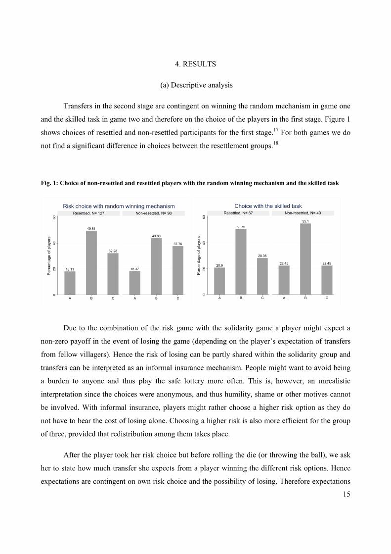
15
4. RESULTS
(a) Descriptive analysis
Transfers in the second stage are contingent on winning the random mechanism in game one
and the skilled task in game two and therefore on the choice of the players in the first stage. Figure 1
shows choices of resettled and non-resettled participants for the first stage.17 For both games we do
not find a significant difference in choices between the resettlement groups.18
Fig. 1: Choice of non-resettled and resettled players with the random winning mechanism and the skilled task
Due to the combination of the risk game with the solidarity game a player might expect a
non-zero payoff in the event of losing the game (depending on the player’s expectation of transfers
from fellow villagers). Hence the risk of losing can be partly shared within the solidarity group and
transfers can be interpreted as an informal insurance mechanism. People might want to avoid being
a burden to anyone and thus play the safe lottery more often. This is, however, an unrealistic
interpretation since the choices were anonymous, and thus humility, shame or other motives cannot
be involved. With informal insurance, players might rather choose a higher risk option as they do
not have to bear the cost of losing alone. Choosing a higher risk is also more efficient for the group
of three, provided that redistribution among them takes place.
After the player took her risk choice but before rolling the die (or throwing the ball), we ask
her to state how much transfer she expects from a player winning the different risk options. Hence
expectations are contingent on own risk choice and the possibility of losing. Therefore expectations
18.11
49.61
32.28
18.37
43.88
37.76
020
4060
A B C A B C
Resettled, N= 127 Non-resettled, N= 98
Perc
enta
ge o
f pla
yers
Risk choice with random winning mechanism
20.9
50.75
28.36
22.45
55.1
22.45
020
4060
A B C A B C
Resettled, N= 67 Non-resettled, N= 49
Perc
enta
ge o
f pla
yers
Choice with the skilled task

16
are only available for players who were at risk of losing the risk game (risk option B or C). In line
with our interpretations, we find that higher transfer expectations go along with taking higher risks
(mean expectation of players who chose option B: 643.91 KHR, mean expectation of players who
chose option C: 838.81 KHR, p-value 0.02). Mean expectations differ at the one % significance
level between resettled and non-resettled players (resettled players: 584.28 KHR, non-resettled
players: 905.55 KHR, p-value: 0.00) likely being caused by stronger solidarity in the established
villages.19
Analyzing transfer sending of winners to losers in game one Table 5 shows that mean
transfers of resettled players are significantly lower. The resettled players transfer on average 38%
less money than non-resettled players. Transfer sending decreases with the skill driven winning
mechanism.20 However, the decrease is larger in the resettled village (22%) than in the non-resettled
villages (11%). Thus, individualistic motives of “earning” and “skill” are more important in the
resettled village, while transfers are more unconditional in the non-resettled villages. These findings
were confirmed through qualitative interviews after the experiment. Resettled players reported that
norms of sharing are not present in the new community; as a resettled participant remarked, “Giving
nothing is just the way people behave in this village” (April 4, 2010, session one).
Table 5: Mean transfers in game 1 and game 2 with the skilled task
Resettled players Non-resettled players Obs. Mean
transfers Standard deviation
Obs. Mean transfers
Standard deviation
Significance levela
Game 1 (risk) 456 490.79 711.84 300 792.33 689.49 1% Game 2 (task) 204 381.37 337.54 180 703.61 640.05 1%
Note: a Wilcoxon-Mann-Whitney test for difference in means between resettled and non-resettled players
When we analyze transfers with respect to how much money a potential sender has at hand
(whether the player chose option A or won option B or C) and how high a risk the potential
receiver(s) took (lost option B or option C), we observe the following patterns (see Table C.1 in the
appendix). Firstly, transfer per person was lower to two losers in their group than to one loser
(except the few C-senders who transferred similar amounts no matter whether one or two other

17
players lost) but the total sum of transfers is bigger in the case of two losers. Secondly, even though
absolute transfers increased with the available budget, A-senders were willing to give, with an
average of 14.19%, the highest proportion of their earning (283.76 KHR), followed by B-senders
(9.52%, 628.26 KHR) and C-senders (6.94%, 1,250 KHR).21 Higher relative contributions of less
wealthy people are also found in public good games (Hofmeyr, Burns, and Visser 2007; Buckley
and Croson 2006). Thirdly, there is no evidence that senders discriminate over the risk choice of the
loser. This holds both in resettled and non-resettled communities. Contrary to Trhal and
Radermacher (2009) who played with German university students, we find no evidence that wealthy
individuals help less if they realize that neediness is self-inflicted. Given the importance of 'fate' in
asian countries this seems not too surprising. High risk participants who are incautious are not
“punished” with lower transfers. Average sending to C-losers has a tendency to be lower but this
difference is small and insignificant. We also do not find any evidence of homophily or in-group
bias with higher transfer sending towards people with the same risk choice. If high risk investments
are insured the same way as low risk investments there does not seem to be an innovation bias
caused by a lack of insurance.
Fig. 2: Transfer payments to one B-loser in game 1
Figure 2 shows the cumulated density function of potential transfers to one B-loser for
resettled and non-resettled players. The curve for the resettled players lies entirely above that for the
Non-resettled players
Resettled players
14 % get more than 1,000 KHR
41 % get more than 1,000 KHR
.1
.2
.3
.4
.5
.6
.7
.8
.9
1
Per
cent
age
of lo
sers
0 500 1,000 2,0001,500Transfer to one B-loser

18
non-resettled players. Hence, for the whole distribution of transfers, resettled players were more
likely to receive lower transfers. In the non-resettled group the probability of getting no transfers is
less than 10%, whereas for the resettled players it is close to 20%. Taking a transfer of 1,000 KHR
as an example, only 14% of the resettled players received a higher transfer. The proportion of
players receiving a transfer of more than 1,000 KHR increases to 41% in the group of non-resettled
players.
(b) Transfer differences contingent on risk choice and expectations
Since transfer decisions depend on own and others’ risk choices, simple descriptive analysis
can be misleading. We estimate solidarity conditional on a specific risk choice, to control for
potentially higher transfers made by risk-loving individuals, by including dummy variables for the
type of sender and the type of receiver of the transfer.22 We estimate Tobit regressions as our latent
variable (willingness to support) is expressed by the left censored variable transfer payments with
24% of all observations censored at zero. Table 6 contains the results of Tobit regressions on the six
transfer choices that every winner of a risk game made for all possible types of losers in that
person’s group. Individual socio-demographic controls and session size are included in all
regressions.
We focus on the transfer difference between resettled and non-resettled players. We start by
analyzing only the transfer decisions in game one with the random winning mechanism (regression
(1), N= 126, observations= 756). Here, the resettlement dummy is negative and significant at the
five % level. In a second step, we estimate a random effects Tobit regression which also includes the
transfer decisions in game two with the skilled task (regression (2), N= 156, observations= 1,140).
The resettlement dummy increases in magnitude and remains negatively significant at the one %
level.
The solidarity experiment further includes elements of trust, since transfers depend on
expectations about the solidarity of others (Selten and Ockenfels, 1998). To separate the effects of
solidarity from reciprocal motives, we include transfer expectations in regression (3) (N= 112,
observations= 810). These have a significant positive influence on transfers, confirming the results
of Selten and Ockenfels (1998). The more interesting finding, however, is that resettlement remains
negatively significant. That is, lower transfers are driven not only by lower expectations about the
support of others, but also by a preference for not helping people in the resettled village.23

19
Table 6: Multivariate analysis explaining transfers (marginal effects)
(1) (2) (3) (4) (5) (6)
Tobit regression+
Random-effects Tobit
regression++
Random-effects Tobit regression++
Random-effects Tobit regression++
Random-effects Tobit regression++
Random-effects Tobit
regression++
VARIABLES Transfers game 1
(risk choice)
Transfers game 1 and
2 (skilled task)
Transfers game 1 and 2 (skilled task) for B- and C-
senders
Transfers game 1 and 2 (skilled task)
Transfers game 1 and
2 (skilled task)
Transfers game 1 and
2 (skilled task)
Resettlement -371.6** -549.7*** -413.9** -590.6*** -556.8*** -514.5***
(179.9) (151.5) (197.6) (140.6) (160.3) (152.2)
Skilled task -100.9*** -186.2*** -100.1*** -107.9*** -106.2***
(28.93) (40.53) (28.92) (30.00) (30.03)
Transfer 0.424*** expectations (0.137) Controls for session network
Yes Yes Yes No Yes No
Controls for sender and receiver type
Yes Yes Yes Yes No No
Individual controls
Yes Yes Yes Yes Yes No
Observations 756 1,140 810 1,140 1,140 1,140
Number of individuals
126 156 112 156 156 156
Notes: Standard errors in parentheses; *** p<0.01, ** p<0.05, * p<0.1 + Standard errors are clustered on the individual level ++ Random effects are implemented on the individual level
The individual covariates used in the regressions can be seen in Table C.2 and the dummies for different sender and receiver combinations in Table C.3 in the appendix. It seems that players who have some savings and those who live in bigger households tend to give less. In addition, players with higher education and those who enjoy regular meals tend to give more.
In regression (4) (N= 156, observations= 1,140) we exclude the controls for the network of
family and friends in the session. The negative coefficient of the resettlement dummy increases, as it
now also accounts for the loss of social relations in the new village (compare regressions (2) and

20
(4)). The increase in the coefficient is merely -40.9 KHR. Thus, we believe that the anonymity of
our experiment cancelled out the effect of familiarity in the session. As a robustness check, we
estimate the average treatment effect on the treated using the relative number of family members
and friends with regard to session size as matching variables to estimate the propensity score (Table
C.4 in the appendix). With all different matching methods we still find a significant negative
coefficient of the resettlement dummy ranging from -163 to -391 KHR. These results show that
unconditional giving is driven not so much by the presence of a personal social network as by
solidarity at the village level. Furthermore, the relatively small influence of number of family
members and friends in the session suggests that anonymity, independence of games and no
communication successfully removed personalized trust motivations from the experiment.
Lastly, we estimate transfers without controlling for the risk choices of senders and receivers,
which gives us the total effect of voluntary resettlement (regression (5), N= 156, observations=
1,140). Since there are no significant differences in risk choices between resettled and non-resettled
players we find hardly any differences between regressions (2) and (5).
Applying regression analysis, taking the risk choice and variation in control variables into
account, the resettlement dummy is significant in all the specifications with a magnitude from
-371.6 KHR to -590.6 KHR. Thus, resettled players transfer between 47% and 75% lower amounts
than non-resettled players in game one (792.3 KHR). The difference between the two groups is
larger than that found by a simple descriptive analysis (38%). Regressions (2) to (5) show a
significant negative coefficient for the skilled task, which confirms our hypothesis that effort and
accountability for the game outcome reduces transfers.24 The magnitude of this coefficient with
-100.9 KHR in regression (2) is more than five times smaller than the resettlement effect.25
Confirming our descriptive results we do not find in-group bias or significant discrimination with
respect to risk taking of the loser for all three sender groups.26
It is interesting to note that households that have some savings transfer significantly lower
amounts in all regressions. This is in line with findings that individuals with financial resources face
heavy demands from relatives and friends to share their fortune and therefore use saving schemes to
hide their wealth. In Africa, for example, women especially are willing to entrust their money to
“susu men” in order to withdraw it from their network (Besley 1995, 2150) or to put it into formal
saving accounts with effectively negative interest rates (Dupas and Robinson 2013). Since non-

21
resettled households are significantly more likely to have savings, these findings reduce the size of
our resettlement effect.
Considering the non-random nature of the resettlement choice, the work of McKenzie,
Stillman, and Gibson (2010) provides some information on the magnitude of the bias. Comparing
income improvements after migration, McKenzie, Stillman, and Gibson (2010) find a 25–35% bias
in OLS regressions with non-experimental data in comparison to experimental migration data. But
even then, the resettlement effect identified in regression (2), with -357.3 KHR and 45% of the
average transfer payment of the non-resettled players in game one (792.3 KHR), is still substantial.
As a further robustness check we follow Altonji, Elder, and Taber (2005) and Bellows and
Miguel (2009) who use the attenuation caused by selection on observables as a guide to the degree
of selection on unobservables. Comparing regression (2) with a resettlement coefficient of -549.7
KHR (including full controls) with regression (6) leading to a resettlement coefficient of -514.5
KHR (without any controls), shows that attenuation is with 35.2 KHR very small. Given these
estimates, the selection on unobservables would need to be 15.62 times stronger than selection on
observed variables in order to compensate the entire resettlement effect. Given the rich set of control
variables this seems highly unlikely.27
(c) Ex post survey data on the importance of network support
When we consider the prevalence of various types of shock – such as bad weather
conditions, livestock disease, severe illness of a household member, or fire or theft destroying a
household’s property – the importance of solidarity for our sample becomes evident. About two-
thirds of the players reported having experienced at least one severe shock during the last two years,
and more than 28% reported several shocks. Furthermore, 97% of these players had experienced
difficulties in coping with these shocks. Taking the monetary transfers in the games as an indicator
of general willingness to support fellow villagers, coping with these shocks in the resettled
community is clearly more difficult.
The importance of solidarity becomes even more pronounced when we look at the poverty
status before and after resettlement of project participants. Before resettlement in 2008, about 85%
of the project households earned less than 1.25 USD per day. In 2010, the proportion increased in
the group of resettled participants to 88%, whereas it decreased in the group of non-resettled

22
participants to 79%. Similarly, there were no income differences in 2008 between the households
which got residential land and those who did not get residential land (see Table 1). After
resettlement in 2010, the yearly household income of resettled beneficiaries was on average about
20% lower than that of non-resettled participants (resettled participants: 1,130.61 USD, non-
resettled participants: 1,429.09 USD, p-value: 0.09). Nevertheless, in our specific case, project
transfers could compensate for the greater vulnerability of resettled players. On average 33.5% of
the yearly income of resettled participants came from project transfers, while in the group of non-
resettled participants project transfers account only for 18% of the average yearly income.
Considering the yearly income per household without transfers, participants in the resettled village
had a 36% lower income than non-resettled participants (resettled participants: 751.19 USD, non-
resettled participants: 1,175.55 USD, p-value: 0.02). Here, 98% of the resettled participants would
have fallen below the poverty line and 86% of the non-resettled beneficiaries. Furthermore, resettled
participants’ income was lower in 2010 than it had been in 2008, whereas for non-resettled
participants it was higher. The resettled participants’ income was probably lower because of time
lost building a new home and new community facilities, but more importantly because of the lack of
social capital. Intuitively, a person’s family and friends, community norms, institutions and
associations constitute an important asset people can call for in a crisis but also in the normal
production process (i.e. knowledge transfer, mutual help in clearing the field, planting, weeding,
harvesting, selling, etc.). As stated by Narayan and Pritchett (1999) “a village’s social capital has an
effect on the incomes of the households in that village, an effect that is empirically large, definitely
social, and plausibly causal”. One year after the land distribution, in both groups agricultural income
is with around 25% of income excluding transfers for the resettled and 30% of income excluding
transfers for the non-resettled project members, the second most important income source. But, non-
resettled participants were earning significantly more income with agricultural production in 2010
(resettled participants: 230.89 USD, non-resettled participants: 164.89 USD, p-value: 0.08).
These findings illustrate the heavy dependence of resettled participants on transfers mainly
coming from the project. It is therefore not surprising that perceived ‘future security’ in 2010 was
weaker in the group of resettled participants (p-value: 0.07). We anticipated that especially after the
end of the project in 2014, when no more transfer could be expected, solidarity and solidarity inside
the new village would become essential for the farmers if they are to succeed.

23
5. CONCLUSIONS
Solidarity is required for the well functioning of communities and even the society as a
whole. But, because other-regarding preferences evolve endogenously depending on the context
(compare for example Ockenfels and Weimann (1999) and Brosig-Koch, Helbach, Ockenfels, and
Weimann (2011) who identify significant differences in solidarity (and cooperation) between East
and West German subject tracing back to opposing economic and social history) close monitoring of
interventions is needed.
The aim of this paper is to investigate systematic the impact of resettlement on the propensity
of individual's to express solidarity norms with fellow villagers. We carry out this investigation in
the context of a unique resettlement project in Cambodia. We conducted a lab-in-the-field
experiment comparing voluntarily resettled and non-resettled participants of a land reform project.
All farmers applied for residential and agricultural land and were hence willing to relocate but
farmers in our control group (non-resettled players) received only agricultural land and were still
living in their villages of origin. Our treatment group (resettled players) received residential as well
as agricultural land and moved to a newly founded village about one year prior to our behavioral
experiment. We conducted a solidarity experiment measuring willingness to transfer money to
anonymous community members and then compare transfer between the resettled village and the
non-resettled villages.
We found that resettled players in the experimental game transferred on average between
47% and 75% lower amounts than non-resettled players. Close to 20% of the losers in the resettled
group received no transfers at all, whereas less than 10% of the non-resettled group received no
transfers. One might argue that non-resettled farmers are richer (given the survey data) and therefore
more likely to transfer money. However, this income effect was not significant for our experimental
participants. On the contrary, we suggest that our analysis estimates a lower bound of the “social
effect of resettlement” carried out in less carefully designed resettlement programs. This is because
we would expect even less giving if (i) resettlement was forced instead of voluntary, (ii) no project
support was offered, (iii) we used an experiment to also measure reciprocal ties, (iv) savings were
equally distributed, or (v) village composition in the non-resettled villages was taken into account,
instead of including only the poorest individuals, since richer community members often constitute
the main source of financial and technological assistance and share their agricultural equipment with
poorer neighbors (Lin 2001). A survey carried out before resettlement indicates that there were no

24
observable differences regarding social integration predating resettlement. Consequently, the
transfer difference is probably caused by voluntary resettlement. We further find that the
resettlement effect remains large and significant when we match participants with respect to their
network size and when we include expectations. Both results support our view that transfer
difference is the result of lower solidarity in resettled communities and that this difference is not
mainly driven by the specific network people have and goes beyond consideration of reciprocity.
We do not find that people “punish” high risk taking; instead, the norm of solidarity applies
similarly to everyone and is on average 10% of available income. However, we find a slight
decrease in solidarity when participants could earn their experimental money.
Our findings on solidarity transfers in the experiment also relate to the lower real world
income of resettled project participants after resettlement. Solidarity transfers are related to ‘social
capital’ which is thought to be an important ingredient for coping with shocks and production
(planting, weeding, harvesting, and selling). Considering the low income level of project
participants, especially in the resettled community, network support plays a vital role. Two-thirds of
all players in our experiment reported experiencing substantial shocks such as bad harvests or illness
since receiving the land from the project. Hence, besides support from their network of family and
friends, willingness to support each other inside the village is a major source of help at the moment.
At the time of our study, reciprocal ties of friendship in the resettled village were not yet established
and solidarity was very low. With the loss of solidarity, our study identifies an important effect of
voluntary resettlement that has not been fully explored up to now. Most likely the lower income of
resettled farmers (although they did not need to commute) is stemming from the lack of mutual aid
in production.
Land reforms are high on the international agenda but studies on their consequences mostly
concentrate on economic variables, revealing mixed results, or on involuntary resettlement.
Therefore, we believe that our study presents useful insights on the social and economic losses
caused by voluntary resettlement within a land reform program. Our results of lower solidarity in
resettled communities complement the analysis of Barr (2003) who finds that resettled players show
lower trust. While trust is important for investment and reciprocal arrangements, solidarity is a
better measure for altruism.
Our findings are relevant for resettlement policies based on the “economics of
compensation”, which often neglect these and other social costs by offering too small compensation

25
amounts. They have important implications for the design of resettlement policies underlining that
the provision of community building measures and their monitoring is mandatory. Moreover, the
availability of insurance against shocks in developing countries and in particular in remote rural
areas is urgently needed. There are several directions for future fruitful research. Monitoring social
changes and their interaction with economic changes over time, both in the medium and in the long
run, would provide deeper guidance for policy makers. Thereby, solidarity and reciprocal relations
within the resettled village, but also the development of networks with the village of origin should
be in the focus.

26
NOTES
1 Unsurprisingly, forced resettlement can lead to a poverty trap consisting of poor harvest and damaged informal risk-
coping networks (Lam and Paul 2013). 2 Somewhat related to the topic of resettlement is the experimental literature on “social distance”, which captures
people’s increased willingness to give when they have clues about nationality, occupation, race, religion (Charness and
Gneezy 2008), or friendship and kinship (Vollan 2011). 3 Barr and Genicot (2008) construct a game in which participants form risk-sharing groups to insure against income
shocks. This study does not explicitly test an effect of resettlement. The authors do not find a significant difference
between resettled and non-resettled players’ willingness to share risks, but they do find that resettled villagers form
significantly larger risk-sharing groups. 4 While reciprocal, incentive-based risk-sharing motives also play a role, altruism seems to explain the largest part of
transfers in previous lab-in-the-field experiments (Leider, Möbius, Rosenblat, and Do 2009; Ligon and Schechter 2012). 5 Furthermore, the risk of losing land mainly through forced eviction because of large infrastructure development
projects is substantial. Amnesty International (2008) estimates that at least 150,000 Cambodians (one % of the rural
population) are living at risk of forced eviction. 6 The average land parcel in Cambodia is 0.69 hectares and small-scale farming is common, with 68% owning less than
0.5 hectares (MoP and UNDP 2007). Since the yearly average rice yield between 2000 and 2008 was 2.26 ton/ hectare
(Yu and Fan 2011), the distributed land parcels provide a good opportunity for the project participants. 7 Out of 1,139 applicants 525 households were selected as land recipients. 8 There is thus no influence of social distance due to variation in nationality, education, occupation, race, or religion
between the two groups. 9 Additionally, we estimate a probit regression that includes those proxies available for 2008 and socio-demographic
information about the households. None of the social variables is found to be significant. We also do not find any
difference at the village level between the non-resettled villages and the newly founded village with regard to
availability of credit, types of shocks, fluctuation inside the villages, income composition, market integration, living
conditions in the village relative to the rest of the country, collective action on the village level, presence of minorities
including religious differences, or availability of insurance. 10 The same holds true if we restrict the sample to those households with panel data. 11 This game was also used by Barr and Genicot (2008) in Zimbabwe. 12 Due to time constraints we could not play a second game in all sessions. 13 Gneezy, Leonard, and List (2009) do not find any gender differences. In our task men performed slightly better than
women (mean value men: 4.38, mean value women: 3.92) but the difference is only significant at the 10% level. We
also do not find a correlation between performance in the task and age. 14 The experimental protocol and posters used for visualization are included in appendix D and E at the end of the
dissertation.

27
15 Even though, this risk game is independent from the actual game, we controlled for the outcome of this game in
another specification. All results remained robust and no significant influence of the outcome is identified. 16 The non-resettled players also reported a slightly higher number of players they disliked in their session. As there
were only three non-resettled and two resettled players who disliked other players, we do not discuss the possible
consequences of this. 17 We assume an ordinal scale: option A=1, option B= 2, and option C= 3. 18 We use the Wilcoxon-Mann-Whitney test, t-test, or test of proportions to compare resettled and non-resettled
players and the Wilcoxon signed rank sum test to compare the behavior of players over the two games. 19 Additional information on the risk choice with the skilled task is provided in appendix B. 20 As there is no significant difference between the mean risk choices of resettled and non-resettled players in both
games, we only report mean solidarity transfers independent of the risk choice. But also comparing those players who
made the same risk choice in game one and in the skilled task shows a significant reduction in transfer sending (N=
21, game one: 638.89, skilled task: 607.14, p-value: 0.02). Regression analysis controls for the type of sender. Graphs
of the transfer difference between resettled and non-resettled players in game one and in the skilled task are shown in
Figures C.1, C.2 and C.3 in the appendix. In all risk groups in game one, considerably more resettled players sent no
transfer than non-resettled players. 21 Figure C.1 in the appendix shows a Gaussian probability curve for the relative transfers from the three risk groups.
Even though A-senders have the highest probability of sending no transfer, the above described order of relative
transfers becomes evident for transfers bigger than 0.3% of the payoff. 22 In total 17 dummies are considered. The coefficients of the dummies and other control variables are presented in
Tables C. 2 and C. 3 in the appendix. 23 The resettlement coefficient also remains significant and of relevant size if we run the estimation only on A-senders
which are non-randomly determined as winners (-345.9 Riel on the 1% significance level) and if we run the
estimation on B- and C- senders excluding expectations for which winning is randomly determined (-529.3 Riel on
the 1% significance level). 24 We test also for heterogeneity of treatment effects for resettlement by stepwise including interaction terms between
resettlement status and all socio-demographic variables included in our regression. We also test an interaction term
between resettlement and the skilled task. All interaction terms turn out to be insignificant. 25 As robustness check we follow Cameron and Trivedi (2009). The resettlement effect remains significant when by
exclude the upper five % of transfer sending, when we use the natural logarithm and estimate with Tobit or OLS
specification. The effect also holds when we separate censored data from non-censored data using two specifications.
Firstly, we estimate a two-part model which models the decision to send transfers as a logit estimation and secondly
the level of transfers conditional on the transfer being non-zero as an OLS estimation. Secondly, we estimate the
same decisions with a Heckman selection model. In both cases the resettlement dummy is negatively significant for
the decision to send transfers and negatively significant for the level of transfers. 26 Mean comparison tests for all three sender types over adequate receiver types are insignificant in all regressions.

28
27 Including the controls for sender and receiver types the resettlement coefficient is with -508.51 only slightly smaller
than without any controls. Here attenuation caused by unobservables would have to be 13.35 times bigger to explain
away the resettlement effect.
29
REFERENCES
Abutte, Wolde-Selassie 2000. Social re-articulation after resettlement: Observing the Beles valley
scheme in Ethiopia. In Risks and reconstruction: Experiences of resettlers and refugees,
edited by Michael M. Cernea and Christopher McDowell. Washington: The World Bank:
412-430.
Albertus, Michael, and Oliver Kaplan. 2013. Land Reform as a Counterinsurgency Policy
Evidence from Colombia. Journal of Conflict Resolution 57 (2):198-231.
Altonji, Joseph G., Todd E. Elder, and Christopher R. Taber. 2005. Selection on observed and
unobserved variables: Assessing the effectiveness of Catholic schools. Journal of political
economy 113 (1):151-184.
Amnesty International. 2008. Rights Razed; Forced evictions in Cambodia. Available from:
http://www.amnesty.org/en/library/asset/ASA23/002/2008/en/b1328237-07c2-11dd-badf-
1352a91852c5/asa230022008eng.pdf (accessed 06.02.2013).
Attanasio, Orazio, Abigail Barr, Juan-Camilo Cardenas, Garance Genicot, and Costas Meghir.
2012. Risk Pooling, Risk Preferences, and Social Networks. American Economic Journal:
Applied Economics 4 (2):134-167.
Bardsley, Nicholas. 2008. Dictator game giving: altruism or artefact? Experimental Economics 11
(2):122-133.
Barr, Abigail. 2003. Trust and Expected Trustworthiness: Experimental Evidence from
Zimbabwean Villages. The Economic Journal 113 (489):614-630.
Repeated Author. 2004. Forging Effective New Communities: The Evolution of Civil Society in
Zimbabwean Resettlement Villages. World Development 32 (10):1753-1766.
Barr, Abigail, Marleen Dekker, and Marcel Fafchamps. 2010. The formation of community based
organizations in sub-Saharan Africa:An analysis of a quasi-experiment. Economic and
Social Research Council (UK).
Barr, Abigail, and Garance Genicot. 2008. Risk Sharing, Commitment and Information: An
experimental analysis. Journal of the European Economic Association 6 (6):1151-1185.

30
Bellows, John, and Edward Miguel. 2009. War and local collective action in Sierra Leone.
Journal of Public Economics 93 (11):1144-1157.
Berg, Todd M. V. 1999. “We Are Not Compensating Rocks”: Resettlement and Traditional
Religious Systems. World Development 27 (2):271-283.
Besley, Timothy. 1995. Savings, Credit and Insurance. In Handbook of Development Economics,
edited by J. Behrman and T. N. Srinivasan. Amsterdam: North-Holland Press.
Binswanger, Hans P. 1981. Attitudes Toward Risk: Theoretical Implications of an Experiment in
Rural India. The Economic Journal 91 (364):867-890.
Repeated Author. 1980. Attitudes Toward Risk: Experimental Measurement in Rural India.
American journal of agricultural economics 62 (3):395-407.
Brosig-Koch, Jeannette, Christoph Helbach, Axel Ockenfels, and Joachim Weimann. 2011. Still
different after all these years: Solidarity behavior in East and West Germany. Journal of
Public Economics 95 (11):1373-1376.
Buckley, Edward, and Rachel Croson. 2006. Income and wealth heterogeneity in the voluntary
provision of linear public goods. Journal of Public Economics 90 (4–5):935-955.
Cameron, Adrian C., and Pravin K. Trivedi. 2009. Microeconometrics using stata. Vol. 5: Stata
Press College Station, TX.
Carpenter, Jeffrey, Allison Liati, and Brian Vickery. 2010. They Come To Play. Rationality and
Society 22 (1):83-102.
Charness, Gary, and Uri Gneezy. 2008. What's in a name? Anonymity and socialdistance in
dictator and ultimatumgames. Journal of Economic Behavior and Organization 68 (1):29-
35.
Cherry, Todd, Peter Frykblom, and Jason F. Shogren. 2002. Hardnose the Dictator. The American
Economic Review 92 (4):1218-1221.
Cherry, Todd, and Jason F. Shogren. 2008. Self-interest, sympathy and the origin of endowments.
Economics Letters 101 (1):69-72.
Colchester, Marcus. 2004. Conservation policy and indigenous peoples. Environmental Science &
Policy 7 (3):145-153.

31
Cousins, Ben, and Ian Scoones. 2010. Contested paradigms of ‘viability’ in redistributive land
reform: perspectives from southern Africa. Journal of Peasant Studies 37 (1):31-66.
Cox, James C., Daniel Friedman, and Seven Gjerstad. 2007. A tractable model of reciprocity and
fairness. Games and Economic Behavior 59 (1):17-45.
Dekker, Marleen. 2004. Sustainability and Resourcefulness: Support Networks During Periods of
Stress. World Development 32 (10):1735-1751.
Dekker, Marleen, and Bill Kinsey. 2011. Contextualizing Zimbabwe's land reform: long-term
observations from the first generation. The Journal of Peasant Studies 38 (5):995-1019.
Dinh, Quoc H., Thomas B. Dufhues, and Gertrud Buchenrieder. 2012. Do connections matter?
Individual social capital and credit constraints in Vietnam. European Journal of
Development Research 24 (3):337–358.
Dupas, Pascaline, and Jonathan Robinson. 2013. Savings Constraints and Microenterprise
Development: Evidence from a Field Experiment in Kenya. American Economic Journal:
Applied Economics 5 (1):163-192.
Eguavoen, Irit, and Weyni Tesfai. 2012. Social impact and impoverishment risks of the Koga
irrigation scheme, Blue Nile basin, Ethiopia. Afrika Focus 25 (1):39-60.
Eidelson, Roy J., and Judy I. Eidelson. 2003. Dangerous ideas: Five beliefs that propel groups
toward conflict. American Psychologist 58 (3):182-192.
Fafchamps, Marcel, and Flore Gubert. 2007. The formation of risk sharing networks. Journal of
Development Economics 83 (2):326-350.
Fafchamps, Marcel, and Susan Lund. 2003. Risk-sharing networks in rural Philippines. Journal of
Development Economics 71 (2):261-287.
Gneezy, Uri, Kenneth L. Leonard, and John A. List. 2009. Gender Differences in Competition:
Evidence From a Matrilineal and a Patriarchal Society. Econometrica 77 (5):1637-1664.
Goodall, Heather. 2006. Exclusion and re-emplacement: Tensions around protected areas in
Australia and Southeast Asia. Conservation and Society 4 (3):383–395.

32
Henrich, Joseph, Robert Boyd, Samuel Bowles, Colin Camerer, Ernst Fehr, Herbert Gintis, and
Richard McElreath. 2001. In search of homo economicus: behavioral experiments in 15
small-scale societies. The American Economic Review 91 (2):73-78.
Hoffman, Elizabeth, Kevin McCabe, Keith Shachat, and Vernon Smith. 1994. Preferences,
Property Rights, and Anonymity in Bargaining Games. Games and Economic Behavior 7
(3):346-380.
Hofmeyr, Andre, Justine Burns, and Martine Visser. 2007. Income inequality, reciprocity and
public good provision: An experimental analysis. South African Journal of Economics 75
(3):508-520.
Karanth, Krithi K. 2007. Making resettlement work: The case of India’s Bhadra Wildlife
Sanctuary. Biological Conservation 139 (3–4):315-324.
Lam, Lai M., and Saumik Paul. 2013. Displacement and Erosion of Informal Risk-Sharing:
Evidence from Nepal. World Development 43 (0):42-55.
Leibbrandt, Andreas, Uri Gneezy, and John A. List. 2013. Rise and fall of competitiveness in
individualistic and collectivistic societies. Proceedings of the National Academy of
Sciences 110 (23):9305-9308.
Leider, Stephen, Markus M. Möbius, Tanya Rosenblat, and Quoc-Anh Do. 2009. Directed
Altruism and Enforced Reciprocity in Social Networks. The Quarterly Journal of
Economics 124 (4):1815-1851.
Ligon, Ethan, and Laura Schechter. 2012. Motives for sharing in social networks. Journal of
Development Economics 99 (1):13-26.
Lin, Nan. 2001. Social capital: Theory and Research. Cambridge: Cambridge University Press.
Margolius, Cheryl, John Beavers, and Marie C. Paiz. 2002. Relocating People Out of Private
Reserves Voluntary Resettlement as a Conservation Tool in Guatamala. Conservation in
Practice 3 (2):30-33.
Mason, T. David. 1986. Land reform and the breakdown of clientelist politics in El Salvador.
Comparative Political Studies 18 (4):487-516.
Repeated Author. 1998. “Take Two Acres and Call Me in the Morning”: Is Land Reform a
Prescription for Peasant Unrest? The Journal of Politics 60 (1):199-230.
33
McCulloch, Neil, and Bob Baulch. 2000. Simulating the impact of policy upon chronic and
transitory poverty in rural Pakistan. The Journal of Development Studies 36 (6):100-130.
McKenzie, David, Steven Stillman, and John Gibson. 2010. How Important is Selection?
Experimental VS. Non-Experimental Measures of the Income Gains from Migration.
Journal of the European Economic Association 8 (4):913-945.
MoP, and UNDP. 2007. Expanding Choices for Rural Cambodia. In Cambodian Human
Development Report. Phnom Penh: Ministry of Planning Cambodia and United Nations
Development Programme Cambodia.
Morris-Jung, Jason, and Robin Roth. 2010. The Blurred Boundaries of Voluntary Resettlement: A
Case of Cat Tien National Park in Vietnam. Journal of Sustainable Forestry 29 (2-4):202-
220.
Narayan, Deepa, and Lant Pritchett. 1999. Cents and sociability: Household income and social
capital in rural Tanzania. Economic Development and Cultural Change 47 (4):871–897.
Ockenfels, Axel, and Joachim Weimann. 1999. Types and patterns: an experimental East-West-
German comparison of cooperation and solidarity. Journal of Public Economics
(71:2):275-287.
Okten, Cagla, and Una O. Osili. 2004. Social Networks and Credit Access in Indonesia. World
Development 32 (7):1225-1246.
Ravallion, Martin, and Binayak Sen. 1994. Impacts on rural poverty of land-based targeting:
further results for Bangladesh. World Development 22 (6):823-838.
Rogers, Sarah, and Mark Wang. 2006. Environmental Resettlement and Social Dis/Rearticulation
in Inner Mongolia, China. Population and Environment 28 (1):41-68.
Schmidt-Soltau, Kai, and Dan Brockington. 2007. Protected Areas and Resettlement: What Scope
for Voluntary Relocation? World Development 35 (12):2182-2202.
Schmidt–Soltau, Kai. 2003. Conservation–related Resettlement in Central Africa: Environmental
and Social Risks. Development and Change 34 (3):525-551.
Selten, Reinhard, and Axel Ockenfels. 1998. An experimental solidarity game. Journal of
Economic Behavior and Organization 34 (4):517-539.

34
Tefera, Messay M. 2009. Challenges and opportunities of voluntary resettlement schemes in
Ethiopia: A case frm Jiru Gamachu resettlement village, Nonno district, Central Ethiopia.
Journal of Sustainable Development in Africa 11 (3):83-102.
Trhal, Nadja, and Ralf Radermacher. 2009. Bad luck vs. self-inflicted neediness - An
experimental investigation of gift giving in a solidarity game. Journal of Economic
Psychology 30 (4):517-526.
Valente, Christine. 2009. The food (in) security impact of land redistribution in South Africa:
microeconometric evidence from national data. World Development 37 (9):1540-1553.
Vollan, Björn. 2011. The difference between kinship and friendship: (Field-) experimental
evidence on trust and punishment. Journal of Socio-Economics 40 (1):14-25.
Yu, Bingxin, and Shenggen Fan. 2011. Rice production response in Cambodia. Agricultural
Economics 42 (3):437-450.
Zhang, Yong, Daming He, Ying Lu, Yan Feng, and Jake Reznick. 2013. The influence of large
dams building on resettlement in the Upper Mekong River. Journal of Geographical
Sciences 23 (5):947-957.
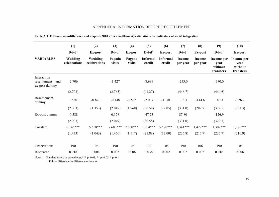
35
APPENDIX A: INFORMATION BEFORE RESETTLEMENT
Table A.1: Difference-in-difference and ex-post (2010 after resettlement) estimations for indicators of social integration
(1) (2) (3) (4) (5) (6) (7) (8) (9) (10)
D-i-d+ Ex-post D-i-d+ Ex-post D-i-d+ Ex-post D-i-d+ Ex-post D-i-d+ Ex-post VARIABLES Wedding
celebrations Wedding
celebrations Pagoda
visits Pagoda visits
Informal credit
Informal credit
Income per year
Income per year
Income per year
without transfers
Income per year
without transfers
Interaction resettlement and ex-post dummy
-2.706 -1.427 -8.999 -253.0 -370.0
(2.703) (2.765) (41.27) (446.7) (444.6) Resettlement dummy 1.830 -0.876 -0.148 -1.575 -2.007 -11.01 138.3 -114.6 143.3 -226.7
(2.003) (1.353) (2.049) (1.968) (30.58) (22.05) (331.0) (282.7) (329.5) (281.3) Ex-post dummy -0.588 0.178 -47.73 87.80 -126.9
(2.003) (2.049) (30.58) (331.0) (329.5) Constant 6.146*** 5.558*** 7.683*** 7.860*** 100.4*** 52.70*** 1,341*** 1,429*** 1,302*** 1,176*** (1.433) (1.043) (1.466) (1.517) (21.88) (17.00) (236.8) (217.9) (235.7) (216.9)
Observations 190 106 190 106 190 106 190 106 190 106
R-squared 0.018 0.004 0.005 0.006 0.036 0.002 0.002 0.002 0.016 0.006Notes: Standard errors in parentheses;*** p<0.01, ** p<0.05, * p<0.1 + D-i-d= difference-in-difference estimation

36
Table A.2: Test for equality of the coefficients of the difference-in-difference and the ex-post estimation
Interaction resettlement and ex-post dummy of
d-i-d estimation
Resettlement dummy of ex-
post estimation
Significance level of test for equality
Wedding celebrations -2.706 -0.876 n.s.a
Pagoda visits -1.427 -1.575 n.s. Informal credit -8.999 -11.01 n.s. Income per year -253.0 -114.6 n.s. Income per year without transfers -370.0 -226.7 n.s.
Notes: a n.s. not signifcant
APPENDIX B: RISK CHOICE IN GAME TWO AND WITH THE SKILLED TASK
In game two, the average risk choice in the skilled task is significantly lower than the
average risk choice in game one (game one: 2.19, game two: 2.04, p-value: 0.05, see also Fig. 1).
This reduction is driven by the less confident non-resettled players who decreased their risk
significantly (non-resettled: game one: 2.24, game two: 2.00, p-value: 0.02; resettled: game one:
2.14, game two: 2.07, p-value: 0.54). There is no significant difference in risk choice with the
skilled task between resettled and non-resettled players (resettled: 2.07, non-resettled: 2.00, p-
value: 0.56), but actual skills are significantly higher in the non-resettled group (mean times a
player got the ball into the bucket: resettled: 3.79, non-resettled: 4.51, p-value: 0.02). This means
that 10% of the resettled players underestimated their skill and 48% overestimated it, whereas
16% of the non-resettled players underestimated their skill and only 37% overestimated it. These
findings hint at overconfidence especially among the resettled players.

37
APPENDIX C: ADDITIONAL ANALYSES ON TRANSFER SENDING
Table C.1: Mean transfer per person dependent on risk choices of winners and losers in game 1
1 B-loser
1 C-loser
2 B-losers
2 C-losers
2 losers: 1 B- and 1 C-loser;
transfer to the B-loser
2 losers: 1 B- and 1 C-loser; transfer to the
C-loser
Average over
senderA-sender 328.21 323.08 255.13 264.38 264.10 266.67 283.76 B-sender 752.17 692.75 581.16 569.57 605.80 568.12 628.26 C-sender 1,222.22 1,277.78 1,277.78 1,194.44 1,250.00 1,277.78 1,250.00 Average over receiver
688.09 661.90 579.76 564.68 592.06 576.19 -
Significance levelb n.s. n.s. 10% -
Notes: b Wilcoxon-Mann-Whitney, t-test, or test of proportions for difference in means between resettled and non-resettled players
Fig. C.1: Transfer payments according to risk choices in game 1
54.55
22.73
13.649.091 11.76
17.65
52.94
17.65
010
2030
4050
60
0 1,000 2,000 3,000 0 1,000 2,000 3,000
Resettled, N= 22 Non-resettled, N= 17
Per
cent
age
of p
laye
rs
Transfer to one B-loser
Risk option A
28.89
6.667
35.56
17.78
8.8892.222
16.6720.83
25
4.167
12.516.67
4.167
010
2030
4050
60
0 1,000 2,000 3,000 0 1,000 2,000 3,000
Resettled, N= 45 Non-resettled, N= 24
Per
cent
age
of p
laye
rs
Transfer to one B-loser
Risk option B
37.5
12.5
37.5
12.5 11.11
44.44
11.11
33.33
010
2030
4050
60
0 1,000 2,000 3,000 0 1,000 2,000 3,000
Resettled, N= 9 Non-resettled, N= 9
Per
cent
age
of p
laye
rs
Transfer to one B-loser
Risk option CC-sender B-sender
A-sender
.2
.4
.6
.8
1
Per
cent
age
of lo
sers
0 .1 .2 .3 .4 .5Transfer to one B-loser in round 2 realtive to earnings

38
Fig. C.2: Gaussian probability curves of transfer payments in game 1 of resettled and non-resettled players
0
.2
.4
.6
.8
1
0 500 1,000 1,500 2,000Transfer to 1 B-loser
0
.2
.4
.6
.8
1
0 500 1,000 1,500 2,000Transfer to 1 C-loser
0
.2
.4
.6
.8
1
0 500 1,000 1,500 2,000Transfer to B-loser: 2 B-losers
0
.2
.4
.6
.8
1
0 500 1,000 1,500 2,000Transfer to B-lose: 1 B- and 1 C-loser
Per
cent
age
of lo
sers
0
.2
.4
.6
.8
1
0 500 1,000 1,500 2,000Transfer to C-loser: 1 B- and 1 C-loser
0
.2
.4
.6
.8
1
0 500 1,000 1,500 2,000Transfer to C-loser: 2 C-losers
Solid line= resettled players, N= 76; Dashed line= non-resettled players, N= 50
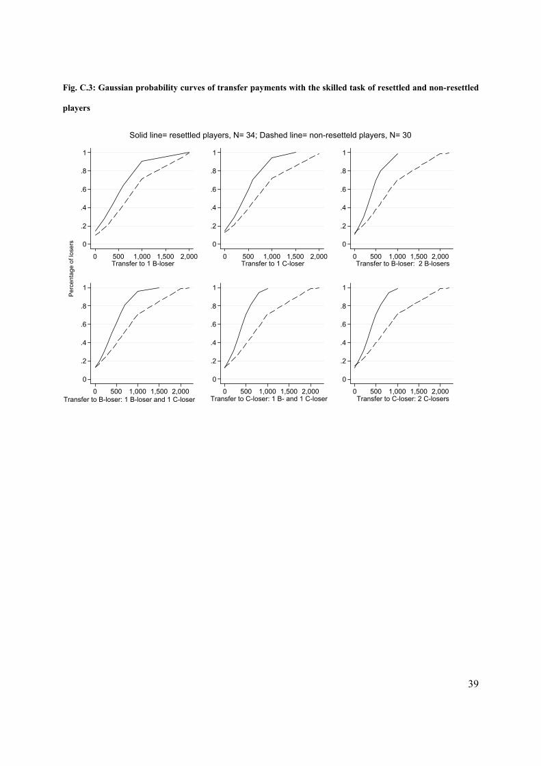
39
Fig. C.3: Gaussian probability curves of transfer payments with the skilled task of resettled and non-resettled
players
0
.2
.4
.6
.8
1
0 500 1,000 1,500 2,000Transfer to 1 B-loser
0
.2
.4
.6
.8
1
0 500 1,000 1,500 2,000Transfer to 1 C-loser
0
.2
.4
.6
.8
1
0 500 1,000 1,500 2,000Transfer to B-loser: 2 B-losers
0
.2
.4
.6
.8
1
0 500 1,000 1,500 2,000Transfer to B-loser: 1 B-loser and 1 C-loser
0
.2
.4
.6
.8
1
0 500 1,000 1,500 2,000Transfer to C-loser: 1 B- and 1 C-loser
0
.2
.4
.6
.8
1
0 500 1,000 1,500 2,000Transfer to C-loser: 2 C-losers
Solid line= resettled players, N= 34; Dashed line= non-resetteld players, N= 30
Per
cent
age
of lo
sers

40
Table C.2: Individual control variables for the transfer regressions in table 6
VARIABLES (1) (2) (3) (4) (5)
Gender of experimental participant -74.77 -108.0 -151.0 -114.0 -92.66
(1= female, 0= male) (159.4) (134.9) (177.8) (133.3) (143.4)
Age 2.887 3.278 1.814 3.188 3.016
(6.514) (6.085) (7.949) (6.101) (6.393)
Years of education 65.74** 45.70* 46.03 45.97* 56.00**
(26.05) (26.59) (33.84) (26.67) (28.09)
Household size -61.73 -91.25*** -62.24 -86.00** -93.14**
(37.89) (35.06) (46.40) (34.79) (36.88)
Married+ 198.1 139.7 237.8 136.5 106.0
(163.7) (163.4) (202.5) (163.8) (172.2)
Income per month -0.101 0.147 -0.329 0.0631 0.0270
(0.650) (0.713) (1.002) (0.710) (0.755)
Nutrient provision++ 428.1** 360.6** 284.4 339.0** 384.7**
(173.6) (141.7) (189.4) (139.5) (149.6)
Savings+ -378.3*** -373.4*** -467.1** -358.6*** -398.7***
(142.9) (137.1) (186.1) (136.4) (144.9)
More than 50 USD debt+ 39.64 146.4 87.57 134.4 189.0
(131.7) (136.9) (185.6) (136.8) (144.6)
Shock during the last 3 years+++ -83.75 -26.84 106.6 -13.08 -37.04
(123.3) (137.3) (167.5) (136.9) (145.2)
Shocks of friends or family+++ 272.4* 157.8 196.1 156.5 131.5
(148.4) (132.1) (163.1) (132.3) (140.1)
Relative number of friends++++ 0.761 3.653 0.0750 4.613
(4.435) (3.838) (5.164) (4.057)
Relative number of family members++++
1.834 0.735 -5.043 0.158
(7.335) (7.358) (10.46) (7.774)
Responsibility for own fate+++++ 114.7 121.7 70.57 121.5 147.8
(118.6) (122.0) (159.8) (122.1) (129.2)
Always somebody in the village who -123.3 -98.47 -147.4 -93.01 -89.97
helps +++++ (109.6) (111.2) (141.3) (111.3) (118.1)
Session size -13.78 13.71 2.698 19.07 11.42
(36.13) (27.33) (33.64) (26.88) (29.06)

41
Notes: Standard errors in parentheses, *** p<0.01, ** p<0.05, * p<0.1 + Dummy variable: (1= yes, 0= no) ++ Average number of meals with enough food for all household members during the last month +++ “Shock” refers to illness, accident, fire, theft, natural disaster ++++ In relation to the session size +++++ 1= strongly agree - 4= strongly disagree
Table C.3: Sender and receiver dummies for the transfer regressions in table 6
VARIABLES (1) (2) (3) (4) (5)
Sender A & receiver C -5.927 -30.43 -70.17 -30.42
(34.42) (56.92) (118.7) (56.92) Sender A & 2 receivers B B - receiver B -84.87*** -91.93 -99.39 -91.89
(29.54) (57.13) (118.9) (57.12) Sender A & 2 receivers B C - receiver B -74.40** -88.49 -116.2 -88.45
(29.69) (57.12) (119.1) (57.11) Sender A & 2 receivers - B C receiver C -71.41** -88.49 -124.6 -88.45
(34.25) (57.12) (119.1) (57.11) Sender A & 2 receivers C C - C receiver -72.90** -89.63 -124.6 -89.60
(30.85) (57.12) (119.1) (57.12) Sender B & receiver B 426.7*** 323.5*** 251.2** 324.8***
(149.8) (68.02) (125.0) (68.01) Sender B & receiver C 362.6** 266.9*** 195.1 268.2***
(149.6) (68.06) (125.0) (68.05) Sender B & 2 receivers B B - receiver B 241.3* 141.9** 57.79 143.1**
(139.3) (68.17) (125.1) (68.16) Sender B & 2 receivers B C - receiver B 268.2* 173.8** 95.26 175.1**
(142.6) (68.14) (125.1) (68.13) Sender B & 2 receivers B C - receiver C 227.1 127.5* 42.05 128.8*
(142.6) (68.18) (125.1) (68.17) Sender B & 2 receivers C C - receiver C 228.7 122.8* 44.47 124.0*
(141.8) (68.19) (125.1) (68.18) Sender C & receiver B 863.7*** 243.9* 161.1 250.2**
(324.4) (127.7) (173.5) (127.5) Sender C & receiver C 921.9*** 292.9** 212.9 299.1**

42
(338.5) (127.6) (173.3) (127.4) Sender C & 2 receivers B B - receiver B 921.9*** 298.3** 218.6 304.6**
(351.3) (127.6) (173.3) (127.4) Sender C & 2 receivers B C - receiver B 892.8** 271.2** 189.9 277.4**
(356.7) (127.6) (173.4) (127.5) Sender C & 2 receivers B C - receiver C 921.9** 298.3** 218.6 304.6**
(359.6) (127.6) (173.3) (127.4) Sender C & 2 receivers C C - receiver C 834.6** 216.6* 132.2 222.9*
(358.3) (127.7) (173.5) (127.6) Notes: Standard errors in parentheses, *** p<0.01, ** p<0.05, * p<0.1
Table C.4: Transfer differences based on matching results according to the network size in the sessions
Obs. resettled players
Obs. non-resettled
players
Average treatment effect on the treated* Std. err.
T-value
Stratification method 456 294 -283.07 58.20 -4.86Nearest neighbour (random draw) 456 180 -391.62 81.88 -4.78Kernel matching (with bootstrapping, repetitions 50) 456 300 -314.59 145.34 -2.16
Radius matching (0.01) 390 192 -163.20 72.33 -2.26
Notes: * If the common support option is specified the average treatment effect on the treated is also significant for all matching methods.
Table C.5: Transfer differences based on matching results according to income
Obs. resettled players
Obs. non-resettled
players
Average treatment effect on the treated* Std. err.
T-value
Stratification method 456 300 -297.77 50.60 -5.89 Nearest neighbour (random draw) 456 282 -317.11 56.70 -5.59Kernel matching (with bootstrapping, repetitions 50) 456 300 -300.24 119.17 -2.52
Radius matching (0.01) 456 300 -348.95 55.86 -6.25
Notes: * If the common support option is specified the average treatment effect on the treated is also significant for all matching methods.

THE DANGER OF A RISK-INDUCED POVERTY TRAP: APPLICATION TO
RECENTLY RESETTLED AND NON-RESETTLED COMMUNITIES IN CAMBODIA
SIMONE GOBIEN
Institute for Co-operation in Developing Countries, University of Marburg,
Am Plan 2, 35037 Marburg, Germany
Phone: +49 6421 2823736, Fax : +49 6421 2828912
correspondence to: [email protected]
Abstract In developing countries rural households face a highly insecure environment. Their risk-coping
capacity is often low due to the lack of formal and insufficient informal security networks. This
prevents profitable but risky investments and thereby increases the danger of a risk-induced poverty
trap where households get caught in low-risk low-profit activities. This mechanism can be reinforced
if negative experiences create path dependency by decreasing people’s willingness to take risks. To
test this, I combined two risk games where the second game incorporated a solidarity stage allowing
for informal transfers from winners to losers of the game in the same village. I compared voluntarily
resettled participants with non-resettled participants in a land allocation project in Cambodia. Both
groups showed a significant path dependency by taking higher risks in cases of previous success but
resettled players reacted less strongly to this stimulus. Moreover, higher transfer expectations
increased the risk choice in the second game. As expectations were significantly lower in the resettled
community this lower chance of sharing risk with third parties led to higher risk aversion. Resettled
players are therefore in greater danger of getting caught in low-risk low-profit activities.
JEL Codes: C93, Q15, R23
Keywords: Risk taking, Risk-sharing networks, Risk-induced poverty trap, Voluntary
resettlement, “Lab-in-the-field experiment”
Acknowledgements: My special thanks go to Michael Kirk and Björn Vollan for comprehensive support and comments. I gratefully acknowledge the opportunity to do research in the LASED project. I thank the Deutsche Gesellschaft für Internationale Zusammenarbeit and the LASED project team of IP/Gopa in Kratie, especially Franz-Volker Müller, Karl Gerner, Pen Chhun Hak, Phat Phalit, Siv Kong, Sok Lina, and Uch Sopheap, for financial, organizational, and logistical support, and Hort Sreynit, Soun Phara, and the team of research assistants for excellent support in the field, and Tom Gobien, Sebastian Prediger, and Susanne Väth for valuable comments.

2
1. Introduction
To make a living, people have to take risks. Moreover, risk taking is a precondition for
development because innovation requires investment, which is in itself a risky activity. Most
people in the developing world live in rural areas earning an income mainly from cultivating
crops and raising livestock. All kinds of risk and uncertainty – unstable weather conditions,
crop and animal diseases, fluctuating international crop prices, illness of household members,
crime and social unrest – strongly affect, or even dominate, farm households’ investment
decisions (Rosenzweig 1988; Dercon 2005).
A risky environment can therefore be seen as a cause of poverty. Firstly, because negative
experiences make people more fearful (e.g. Weinstein 1989) and anxious individuals are
biased in favor of low-risk alternatives (Raghunathan and Pham 1999; Lerner and Keltner
2001). In his seminal study of risk taking in experimental games in developing countries,
Binswanger (1980) finds that players who had consistently won previous games were likely to
take bigger risks in the next game than those who had lost. He concludes that this path
dependency causes farmers to be less willing to invest after a series of droughts than they
normally would on account of their risk preferences. This effect is independent of changes in
income and wealth caused by the weather shock but rather leads to lower future return and
consequently to poverty.
Secondly, people’s risk-coping capacities determine their investment choices and in turn their
income (World Bank 2013). But because poor people are often faced with limited access to
credit, low saving capacity, a thin labor market, lack of formal insurance and insufficient state
support, they easily get stuck in low-risk low-return activities (Lipton 1968; Rosenzweig and
Binswanger 1993; Yesuf and Bluffstone 2009). It has been shown, for example, that fertilizer
use, which increases both the mean and the variance of profits, depends on the ability to cope
with ex post consumption risk (Lamp 2003; Dercon and Christiaensen 2011), and Dercon
(1996) finds up to 20% income loss for farmers who plant safer but low return crops because
they have little chance of sharing risk with third parties.
Informal risk-coping methods – even though they can often smooth only a fraction of income
shocks (Townsend 1994; Morduch 1999) – are frequently the only fallback method which
helps the poor to break out of what can easily become a vicious cycle: unwillingness to take
risks because of low risk-coping capacity leads to low income or income loss, which further
decreases risk-coping capability and increases the unwillingness to take risks. Reciprocal risk-

3
sharing networks, and also zero-interest loans, unconditional gifts and solidarity, are of
immense importance in developing countries (e.g. Morduch 1999; Fafchamps 2008).
Participation in these networks is intrinsically motivated by friendship and kinship, altruism,
inequity aversion or reciprocity (Barr and Genicot 2008). Geographic proximity plays a major
role as risk-sharing networks are commonly found within a neighborhood (Fafchamps and
Lund 2003; Fafchamps and Gubert 2007). Leaving your ancestral environment may lead to
the weakening of social ties. Resettlement can therefore have negative consequences for risk-
coping capacity, which in turn may reduce your willingness to take risks and cause you to be
caught in a risk-induced poverty trap.1
Gobien and Vollan (2013) show for this set-up that solidarity transfers are significantly lower
in the resettled community. This is in line with Dekker (2004), who finds that resettled land
reform beneficiaries in Zimbabwe are more likely to rely on individual risk-coping methods
than non-resettled households, who rely on their network. Similar, Barr (2003) finds that in a
trust experiment the resettled players trust each other significantly less than non-resettled
players. Both Dekker and Barr use data from land reform beneficiaries 20 years after
resettlement. This shows that the loss of social networks can have severe medium- to long-
term consequences. So even if project support could ease the loss in the short term, informal
networks would regain their central role in the medium to long term, and especially after the
project ends in 2014.
To test for the impact of village networks and the importance of risk experience on future risk
choices, I analyzed data from a ‘lab-in-the-field experiment’ played with beneficiaries of a
land allocation project in Cambodia. I compared two groups of farmers. The first group
consisted of ‘resettled farmer’ who had received agricultural land and also voluntarily
participated in a resettlement scheme. Those participants moved about one year prior to my
study to a newly established village. The second group comprised ‘non-resettled famers’ who
received only agricultural land and were still living in their village of origin. In particular, I
tried to shed light on three interrelated research questions: (1) Do farmers who expect high
solidarity from their village network show a greater willingness to take risks? (2) Does past
success within a risky environment influences future risk choices? (3) Do resettled players
react differently to risk experience than non-resettled players?
1 Compare Lam and Paul (2013), who show that involuntarily resettled farmers in Nepal face a high danger of being trapped in poverty because of the loss of their social network.

4
Risk aversion of farmers can be estimated using actual production data (e.g. Antle, 1987; Bar-
Shira et al., 1997). Here, it is difficult to isolate risk preferences from external constraints like
budget limitations or market imperfections (Just and Pope 2003). Experiments can overcome
this problem by using budget-neutral lotteries (Binswanger 1980). My experiment combined
two risk games. In the first risk game, farmers had to choose one of three risky lotteries. In the
second risk game, the same decision was taken in the first stage and combined with a
solidarity game in the second stage (based on the design of Selten and Ockenfels 1998). In the
solidarity game players were randomly grouped into anonymous groups of three. Winners of
the risk game could chose to send a transfer to losers in their solidarity group.
Experimental sessions were restricted to either solely resettled or solely non-resettled project
participants from the same village. As interactions took place between anonymous villagers,
no future interactions were possible, and monetary transfers were not revealed, the solidarity
game captured a village norm of solidarity expressed in the willingness to transfer payments
to anonymous villagers. Solidarity is understood as a kind of informal insurance against
shocks, motivated by pro-social preferences (see Gobien and Vollan 2013 for more details).
Therefore, this set-up enabled me to identify the effect of differences in expected village
solidarity on risk preferences.
I found that solidarity expectations had a positive effect on risk choices in game two.
Expectations were significantly lower for resettled players than for non-resettled players. This
lowered resettled player’s probability of choosing high risk options. Both groups showed
considerable path dependency by choosing higher risks in the event of winning the previous
game. But resettled players reacted less strongly than non-resettled participants. Together,
these results suggest a danger of getting caught in a risk-induced poverty trap for the whole
sample but the danger seems to be higher for resettled than non-resettled households.
Pooled or random effects (RE) models are the techniques most commonly used to analyze
repeated games. But as long as we believe that unobserved time-invariant characteristics –
e.g. probability weighting of risk alternatives or valuation of monetary outcomes – influence
the decision in the game and are correlated with the explanatory variables, those estimates are
inconsistent and fixed effects (FE) models are appropriate. In risk experiments, the latent
variable – risk preferences – is usually modelled in a multivariate ordered framework, which
makes non-linear estimation techniques necessary. In this case, direct FE estimation cannot be
applied. I therefore discussed and compared RE and possible FE estimations for this set-up. I
found that estimates for time-variant effects show the same directions in all specifications but

5
that the relative strength of the coefficients, efficiency of estimates and significance levels
vary between estimation techniques and in particular between RE and FE estimations.
Moreover, a Hausman test strongly rejected the RE specification, which shows that results
differed considerably and FE estimation was appropriate.
The rest of the paper is organized as follows. Section 2 introduces the research setting and
explains how the project beneficiaries were selected, Section 3 presents the survey data on
socio-economic variables before resettlement, Section 4 describes the lab-in-the-field
experiment and my methods of testing the above discussed issues, Section 5 discusses
possible estimation techniques, Section 6 provides the empirical analysis, and Section 7
concludes.
2. Background
The experiment was conducted with beneficiaries of the LASED project (Land Allocation for
Social and Economic Development). LASED is a Royal Government of Cambodia project
supported by the World Bank and GIZ (German Agency for International Cooperation) which
aims to identify a national strategy for allocating land to poor landless and landpoor people
(those with less than half a hectare). Households can apply for agricultural land (between one
and three hectares) or residential land (either 800 or 1200 square meters), or both agricultural
and residential land.
The project is ongoing in several provinces but most advanced in Kratie Province, where my
research was based. The application process started early in 2008. In Kratie Province, only
households in the Sambok and Changkrang Communes of Chetborei District could apply for
project land. The project staff estimated that only one to two percent of eligible households
failed to apply. All applicants were willing to relocate and applied for both residential and
agricultural land but only 52% were granted both types of land. Of the rest, 44% received
only agricultural land and the remaining 4% only residential land.2 There was excess demand
for both agricultural and residential land and applicants were selected according to the degree
of neediness. Households that did not have residential land before the land allocation were
granted residential land. But the socio-demographic characteristics (type of house, income,
land holdings, assets and so on) of the resettled and non-resettled households were very
similar before land allocation (see Table 1).
2 Households that received only residential land are excluded from my analysis as no general statement is possible.

6
By the end of 2008 the first land had been distributed to 525 families. All the residential land
plots were situated in a newly established village and all the agricultural plots were around
this new village. Households that had been allocated residential land moved permanently to
this new village (the resettled group) and households that had been allocated only agricultural
land stayed in their village of origin (the non-resettled group) and had to commute to their
agricultural plots. The location of each household’s residential or agricultural plot was
decided by lottery. At the time of writing, around 10,000 hectares had been allocated by the
LASED project to approximately 5,000 households.
3. Data before resettlement
Selection of beneficiaries of development projects is usually non-random. This makes the
identification of an appropriate control group difficult. Most important in this setting is that
ex-ante risk preferences might differ between recently resettled and non-resettled players.
Voluntary resettlement resembles a migration decision. Jaeger et al. (2010) show that
individuals who are willing to migrate tend to be more risk loving. However, all households
applied for both residential and agricultural land and were hence willing to relocate. The
resettlement decision is therefore not an indicator of different ex-ante risk preferences
between the two groups.
This set-up has the advantage that the project’s beneficiary selection procedure ensured that
the two groups were very similar. Restrictions on the ex-ante poverty status were the same for
both groups and the project selected only households that had been living in the two project
communes before the start of the project. Almost all the beneficiaries had lived in the same
social environment for at least four years, which had enabled them to build stable social
relations in their village of origin. Both groups were motivated to farm and obtained
agricultural land of similar size, located in the same area and consequently of comparable
quality.
The similarity between the two groups was also confirmed by data from my random survey of
84 households in 2008 before the allocation of the land (Table 1). Unfortunately, my survey
did not measure these households’ attitude to risk. Nonetheless, the literature on risk
preferences assumes that some of the available socio-economic variables are determinates of
risk preferences and that others can tell us something about the risk-coping possibilities of the
two groups (see Wik 2004 for a similar discussion).

7
Table 1: Household characteristics before the allocation of land by the project (data from author’s
random household survey of project members in September 2008)
Resettled, N= 43
Non-resettled, N= 41 Difference in meansa
Mean Std dev Mean Std dev Significance level
Wealth indicators
Income per month (USD) 123.30 157.23 111.77 106.87 n.s.b
Land before the project start (hectare) 0.28 0.64 0.27 0.57 n.s.
Savings+ 0.60 0.49 0.59 0.50 n.s.
Nutrient provisionc 5.40 0.53 4.80 0.55 n.s.
Total credit (USD) 169.04 226.59 192.80 242.11 n.s.
Number of cows 0.60 1.48 0.68 1.17 n.s.
Number of radios 0.30 0.51 0.27 0.45 n.s.
Number of TVs 0.42 0.50 0.32 0.47 n.s.
Number of mobile phones 0.26 0.66 0.22 0.47 n.s.
Number of bicycles 0.88 0.82 0.76 0.70 n.s.
Number of motorbikes 0.21 0.41 0.17 0.38 n.s.
Wealth related socio-demographics
Years of education of household head 4.02 0.49 3.78 0.48 n.s.
Age of household head 41.37 9.43 42.17 10.85 n.s.
Household head is married+ 0.81 0.06 0.71 0.07 n.s.
Household size 6.06 2,73 5.48 1.92 n.s.
Housing conditions
Size of the housed 1.46 0.59 1.68 0.72 n.s.
Main material of the roofe 1.51 0.70 1.41 0.67 n.s.
Main material of the exterior wallsf 1.32 0.47 1.27 0.50 n.s.
General condition of the houseg 1.84 0.57 1.90 0.62 n.s.
Variables for social integration
Number of wedding celebrations 6.12 5.23 6.15 5.42 n.s.
Times of visiting the pagoda 7.53 9.61 7.68 7.43 n.s.
Informal credit (USD) 98.41 25.40 100.42 26.96 n.s.
Notes: a Wilcoxon-Mann-Whitney, t-test, or test of proportions for difference in means between resettled and non-resettled households b n.s. not significant c Months enough to eat during the last year d 20 square meters or less (1) / 21–50 square meters (2) / 51 square meters or more (3) e Thatch, palm leaves, plastic sheet, tarpaulin or other soft materials (1) / Corrugated iron (2) / Tiles, fibrous cement, or concrete (3) f Saplings, bamboo, thatch, palm leaves, or other soft materials (1) / Wood, sawn boards, plywood, corrugated iron

8
(2) / Cement, bricks, concrete (3) g In dilapidated condition (1) / In average condition, livable (2) / In good condition and safe (3) + Dummy variable: (1= yes, 0= no)
Wealthier people are believed to be more risk-seeking and probably have better coping
mechanisms. However, there was no significant difference between the two groups in terms of
income, land ownership, savings, nutrient situation, credit and relevant assets. Moreover,
resettled and non-resettled household heads were on average similarly educated and of similar
age. Both variables, education and age of the household head, are likely to be positively
correlated with household wealth and in turn with risk attitude. Getting married and living in a
big household can be interpreted as an increase in labor force, a form of income
diversification, and as providing insurance against shock, which would suggest a positive
correlation with risk as these households might cope better. On the other hand an increase in
household members means a need for more financial resources for food, clothing, education
and so on, which may increase risk aversion. In any case, these two variables did not differ
significantly between the two groups. In addition, three of the available variables suggest a
similar integration into the community before resettlement in 2008 (participation in wedding
celebrations and pagoda visits, which are prominent social events, and availability of informal
credit). It was therefore unlikely that differences in social integration before resettlement
drove risk decisions.
4. Set-up of the experiment
My experiment involved two independent games, played one after the other. Game one
consisted of one risk game and game two then combined the same risk game (stage one) with
a solidarity game (stage two). Players were aware of whether they had won or lost in the
previous game, but their choices of risk and transfer decisions were not revealed to the other
players. Before the start of the first game, I informed the players that, after all the games had
been played, the earnings of only one randomly determined game would be paid out privately
to each player after they had completed a questionnaire.3 The experiment lasted up to half a
day and the average earning per player was equal to the salary for half a day’s wage labor in
this region at this time (4,020 KHR or about 1 USD). In addition, I offered a free meal at the
end of the games instead of a show-up fee.
3 A third game was played which combined a skilled task with the solidarity game. For more details see Gobien and Vollan (2013).

9
4.1 The risk game
The risk game is based on Binswanger (1980, 1981) and follows an ordered lottery selection
design.4 I reduced the risk option to three instead of eight lotteries in order to reduce
complexity in game two where the risk game was combined with a solidarity game.
Participants threw a die to determine the outcome of the risk game.5 Table 2 gives an
overview of the game. Option A is the secure choice, providing a small but secure payoff
(0.50 USD). Option B and C incorporate the risk of losing the game and getting zero payoff,
but they offer a higher expected payoff than option A. Option B has a 2/3 probability of
winning and option C only 1/3. Thus, option A is most attractive to risk-averse players, option
B to players who will take a moderate risk, and option C to risk-loving players. For players
who select option B or C, winning is determined by chance and the sample of winners does
not differ systematically from the sample of losers.
Table 2: Payoffs in the risk experiment
Player’s choice
Probability of high payoff
Die numbers assigned
to high payoff
High payoff in KHR (USD)
Low payoff in KHR (USD)
Expected payoff in KHR (USD)
Option A 1 1, 2, 3, 4, 5, 6 2,000 (0.5) 2,000 (0.5) 2,000 (0.5)
Option B 2/3 3, 4, 5, 6 6,600 (1.65) 0 4,400 (1.10)
Option C 1/3 5, 6 18,000 (4.50) 0 6,000 (1.50)
4.2 The solidarity game
Game two had two stages: the same risk game in stage one and then a one-shot anonymous
solidarity game in stage two. In the solidarity game, three randomly chosen players formed a
solidarity group. Decisions to transfer money were taken after the risk choice only by winners
of the risk game. Players already knew that transfers were going to be made in the event of
there being losers in their three-person group. I applied the strategy methods for transfer
decisions where each player was asked to take a decision for different possible combinations
of a) the number of losers in the player’s group (1 or 2) and b) the risk choice of these losers
(B or C). Hence each player took a total number of six transfer decisions (two decisions if
there was one loser in the group, and four decisions if there were two losers in the group). At
4 It has been used in a field context by Barr and Genicot (2008) in Zimbabwe. 5 Binswanger (1980, 1981) and Barr and Genicot (2008) used a coin toss with equal probability of getting the high or the low payout. This was not possible in my design as the low payout had to be restricted to zero for risk option B and C in order to set a strong and comparable incentive of sending solidarity. The probability of getting the high payout therefore decreased with higher risk.

10
no time did the players know who they were grouped with or how much transfer other players
were willing to give, and communication between the players was prohibited.
4.3 Experimental procedure and participants
The games were played in five villages in the two project communes. This includes the newly
established village (resettled players) and four randomly chosen non-resettled villages.
Between April and May 2010 a total of 16 sessions were carried out – two sessions in each of
the non-resettled villages and eight sessions in the resettled village – with a total of 225
participants (127 resettled players and 98 non-resettled players). Participants were randomly
chosen from a complete list of project beneficiaries but only a maximum of two persons per
household were eligible (persons from the same household did not participate in the same
session). Players had to be at least 18 years old. The experimental participants represented
around 35% of all the project households. None of the players had participated in an
experiment before. The village chief informed the players a few days in advance that they
could participate in an activity in which they could earn money and that they could leave at
any time.
All the sessions took place in the common room of the village community center, where the
instructions were read out to all the players. Decisions were taken in private in a separate
room. All the games were conducted by the same research team and followed a strict protocol.
Instructions were set out on posters explaining the games and cards with this explanation were
handed to the players when they took their decisions.6 Before the first game started, for
practice and to ensure they understood the game, each player threw the die three times and
answered questions about the outcome of the risk game when choosing different risk options.
As Table 3 shows, all players participated in the risk game in game one and game two (N=
225), whereas only those players who won the risk game in the first stage of game two played
the solidarity game in the second stage (N=126).
Table 3: Number of participants in game one and game two
Game one Game two Risk game Stage one:
Risk game Stage two:
Solidarity game Resettled 127 127 76 Non-resettled 98 98 50 Total 225 225 126 6 See appendix D and E of this dissertation for the experimental protocol and the posters.

11
Despite randomization within the two groups, there were fewer households with considerable
savings and more households with considerable credit in the resettled group than in the non-
resettled group (Table 4). These differences might have been caused by resettlement, as
investment needs were higher for resettled project beneficiaries who had to build a house in
the new village. The age structure of resettled and non-resettled players differed, and it
appears there were significantly more shocks in the environment of non-resettled players.
Unsurprisingly, non-resettled players had on average significantly more friends or family
members in their session. I control for these differences in the regression analysis.
Table 4: Individual characteristics of the players from the post-game questionnaire
Resettled, N= 127
Non-resettled, N= 98
Difference in meansa
Mean Std dev Mean Std dev Significance level
Income per month (USD) 124.40 101.89 113.52 85.71 n.s.b
Savings+ 0.27 0.44 0.40 0.49 5%
More than 50 USD debt+ 0.71 0.45 0.50 0.50 1%
Nutrient provision++ 2.65 0.48 2.63 0.48 n.s.
Household size 5.46 1.88 5.74 1.92 n.s.
Gender of participant (1= female, 0= male) 0.58 0.49 0.58 0.49 n.s.
Participant is household head+ 0.48 0.50 0.50 0.50 n.s.
Age 37.08 10.66 41.14 12.31 1%
Married+ 0.77 0.41 0.81 0.38 n.s.
Years of education 3.92 2.75 3.95 2.28 n.s.
Household owns a bicycle+ 0.55 0.50 0.49 0.50 n.s.
Household owns a motorbike+ 0.29 0.46 0.31 0.46 n.s.
Shock during the last three years+ 0.69 0.47 0.63 0.48 n.s.
Shocks of friends or family 0.57 0.50 0.69 0.46 5%
Relative number of friends+++ 10.54 12.00 19.71 22.10 1%
Relative number of family members++ 2.24 5.59 7.47 11.52 1%
Notes: a Wilcoxon-Mann-Whitney, t-test, or test of proportions for difference in means between resettled and non-resettled players b n.s. not significant
+ Dummy variable: (1= yes, 0= no) ++ Average number of meals with enough food for all household members during the last month +++ In relation to the session size

12
4.4 Measuring effects of village networks and path dependency
To test whether farmers who expect higher solidarity from their village network show a
greater willingness to take risks, solidarity expectations in the event of losing are included in
the analysis as an explanatory variable for game two. When players decided on their risk
option in game two they knew that a solidarity game would follow in the second stage. This
might have affected their risk choice as it gave them the opportunity to outsource parts of the
gamble risk. In the first game, the risk of losing was solely carried by the player. With the
introduction of the solidarity game, the risk of losing could be partly shared within the
solidarity group if a player expected to receive a solidarity transfer in the event of losing the
game. Solidarity transfers can thus be interpreted as informal insurance. As risk choices were
not revealed to the other players, the players would not have been inhibited by, for example,
shame or not wanting to be a burden to others, and might have chosen a higher risk option. I
therefore expected that players’ solidarity expectations have a positive influence on their risk
choice in game two.
After taking their risk decision but before throwing the die, players were asked to state how
much transfer they expected from a player winning the different risk options. Thus,
expectations were contingent on the risk choice of losers and could only be recorded for
players who were at the risk of losing (risk option B or C). In addition, I asked separately for
solidarity expectation from different sender types (players who won option A, B, and C) and
distinguished between the cases of one loser and two losers in a group. This leads to a total of
six stated expectations per player.7 To capture as much of the variance in the data as possible,
I use principal component analysis to reduce the data, retaining the principal component with
the highest eigenvalue.8
The second question, if past success within a risky environment influences future risk choices,
is a test for path dependency which might lead to a risk-induced poverty trap. In my
estimations I include a dummy variable for winning the previous game.9 I expected the
dummy to be positive, which would suggest that winners of game one chose to take a higher
risk in game two than losers of game one. An interaction term between a resettlement dummy
7 Namely: An A-sender is confronted with one loser in this group, an A-sender is confronted with two losers in his group, a B-sender is confronted with one loser in this group, a B-sender is confronted with two losers in his group, a C-sender is confronted with one loser in this group, a C-sender is confronted with two losers in his group. 8 See appendix A for more information on the principal component analysis. 9 Other authors add up the scores of the previously won games (e.g. Binswanger 1980; Wik et al. 2004). As I analyze only two games the procedure is comparable.

13
and the winning dummy enables me to test the third hypothesis: Do resettled players react
more weakly to positive risk experience than non-resettled players. If this interaction term is
negative, that would indicate a higher probability of getting caught in low-risk low-return
cycles. In addition, I include a game dummy for game two which captures possible time
effects and the effect of losing the previous game.
5. Estimation strategy
Analyzing experimental data consisting of a combination of several games makes it very
likely we will need individual specific fixed effects.10 This is the case if we assume that
behavioral parameters, like risk preferences, cannot be fully described by a set of observable
explanatory variables. As long as omitted variables are time-invariant, which seems likely
considering the short time span between the games, FE models can correct for this problem.
In addition, despite highly similar socio-economic characteristics of resettled and non-
resettled households before the land allocation (Section 3), unobserved characteristics can
bias the results. The individual fixed effects also account for possible time-invariant
differences between the resettled and the non-resettled players.
FE techniques are non-trivial in ordered response settings. For this reason, I briefly review
possible estimation techniques for ordered categorical panel data that have been suggested in
the literature (Section 5.1) and continue with the implications for this specific research setting
(Section 5.2).11
5.1 Discussion on estimation methods
I want to estimate a latent variable model with ordered response data, given by:
(1)
where represents my main variable of interest – individual risk preferences –of individual i
= 1,…, I at time t = 1,…,T and is a continuous variable which cannot be observed. The vector
of independent explanatory variables is given by , is a random individual-specific
10 An alternative would be to treat the decisions in the two games as representing different behavioural parameters. Then one can use the risk choices from the first game as a regressor in the second game which measures general risk preferences of the players. The advantage of this approach is that ordered logit and probit models are easily implementable. The disadvantage is that endogeneity caused by e.g. omitted variables cannot be addressed. In a setting where two non-randomly formed groups are compared and the behaviour within the game is of interest the latter argument outweighs the former. Nonetheless, the main results hold also for this approach. 11 This cannot be understood as a complete review of possible estimation techniques, but is rather limited to those techniques which seem to be most appropriate for this specific case.

14
effects and is an idiosyncratic error. Since cannot be observed, an ordered response
variable is used with k = 1,…, K categories with specific thresholds of where
:
(2)
Under the assumption that eit is IID (independently and identically distributed), the probability
of observing outcome k of individual i at time t is:
(3) Pr ,
where F(.) is the cumulative distribution function (c.d.f.) of the error term. There are two
standard estimation methods for such a problem: the logit and the probit method, assuming in
the former a logistic c.d.f. and in the latter a standard normal c.d.f. of the error term. In both
cases estimates are obtained by using the maximum likelihood method. Probit and logit
models have similar shapes for central values but differ in the tails. In the ordered response
panel setting, there is little choice between the two methods, because computational
difficulties limit the applicability to panel data and not all estimation commands are
implemented in the standard statistical software.
Depending on the properties of and eit, different estimation methods have to be applied. In
what follows I discuss and compare possible estimation strategies for the ordered response
framework. The first ones allow me to identify time-invariant regressors, most importantly the
resettlement effect, but there is a high probability that they violate the underlying assumptions
and thus produce inconsistent estimates. The other techniques are FE models, which are less
likely to violate their assumptions but can only identify time-variant regressors.
RE models can be used when is purely random, implying that it is not correlated with the
explanatory variables. Under this assumption, estimates of all coefficients – including time-
invariant regressors – are obtained. These estimates are more efficient than those obtained
using FE models, which only use within variation of the data. If the assumption is violated,
then estimates are inconsistent.12
12 Cameron and Trivedi (2009, p.230) emphasize that the FE model is favored in Microeconometrics whereas most other disciplines of applied statistics tend to use RE models. They further propose a pooled model as a natural starting point for linear panel analysis (Cameron and Trivedi 2009, p.244) which leads to consistent estimates if RE models are appropriate. With non-linear estimation techniques this is not the case.

15
The FE model allows a limited form of endogeneity as can be correlated with the
regressors but is still assumed to be uncorrelated.13 Hence, time-invariant components of
the error can be correlated with xit. For example, we assume that if regressors in the risk
regression are correlated with unobserved personality traits, they are correlated only with
time-invariant traits, captured by . In the ordered response setting, inclusion of unobserved
individual heterogeneity is quite complicated. Maddala (1983) has shown that individual fixed
effects lead to inconsistent estimates in a probit setting. I therefore concentrate on the logit
model in the following discussion.
Using a non-linear FE model – such as the ordered logistic estimation technique – two
problems occur when estimating equation (3) (for the following see Baetschmann et al. 2011).
Firstly, only , the difference between the threshold and the fixed effect, can be
identified. The second is the incidental parameter problem (Neyman and Scott 1948) which
states that under fixed T an asymptotic – or in other words, too many individual effects in
short panels – cannot be estimated consistently. This also affects the estimates of β, especially
in short panels where Greene (2004) identified substantial bias.
An easy solution to the problem, proposed by Winkelmann and Winkelmann (1998), is to
transform the ordered response variable into a binary variable such that Chamberlain’s
conditional FE binary logit estimator can be used (Chamberlain 1980). Chamberlain’s
estimator eliminates from the estimation equation by using a log density for the ith
individual that conditions on the sum of outcomes equal to 1 for a given individual over time.
This technique gives a consistent estimate of β for the binary FE logit framework. However,
choice of the threshold is arbitrary and binary treatment of the dependent variable ignores all
variation in yi which takes place below or above the chosen threshold. Individuals who are
constantly coded over time, i.e. their choice of yit is always bigger (or smaller) than the
chosen threshold so that they do not move across the cutoff point, do not contribute to the
likelihood. Hence, some observations are always discarded in the estimation. With substantial
loss of data – as in the study by Winkelmann and Winkelmann (1998), who are left with only
2,523 out of around 10,000 individuals in their sample – the danger that measurement errors
may become a large source of residual variation would be more likely (Ferrer-i-Carbonell and
Frijters 2004).
13 I did not discuss the possibility that eit includes time-varying unobserved factors which are related to observables in an unknown way because under this condition causal inference cannot be made.

16
An alternative to choosing a single cut-off point is the Das and Van Soest (1999) estimator.
These authors propose a two-step method where first the Chamberlain’s estimator is
computed for all K-1 cut-off points and second the estimates are combined, weighted by the
inverse of their variance, which produces the most efficient combination. A serious drawback
of this method is that, in practice, estimation samples for some cut-off points, in particular for
extreme categories, are often small. Here convergence problems and imprecise estimates of
the variance-covariance matrix can occur which force the researcher to limit the analysis to a
subset of possible cut-off points.
Baetschmann et al. (2011) propose a solution for this problem which is based on replicating
the data for each individual K-1 times and each time collapsing the dependent variable at a
different cut-off point. This makes it possible to estimate the model using all K-1 cut-off
points simultaneously, while it imposes the restriction that β2 = β3 =… = βK. The model is
estimated with the Chamberlain approach using clustered standard errors on the individual
level. Baetschmann et al. call this the ‘blow up and cluster’ or BUC estimator. Using Monte
Carlo simulations, they show that the BUC yields consistent and efficient results.
Ferrer-i-Carbonell and Frijters (2004) offer an alternative (called the FF-estimator) which
identifies the optimal cut-off point for each individual such that the individual Hessian matrix,
the second derivative of the log likelihood function, at a preliminary estimate of β is
minimized. This procedure consists of three steps. In the first step, K-1 new binary variables
Dik are produced for each possible cut-off point. In the second step each of these variables is
estimated using the conditional logit approach. Based on the obtained β-coefficients, the
Hessian matrix and the corresponding “trace”, the sum of the diagonal elements of the matrix,
is calculated for each Dik for each individual. The final ‘optimal’ binary variable is based on
the individual Dik with the minimal trace of each individual. In the third step, this variable is
estimated with the conditional logit model and the final β-coefficients are obtained. This
procedure leads to the maximum likelihood estimator with minimal variance, as the variance
of the estimated conditional logit coefficients is the negative of the inverse of the sum of the
Hessian matrix over all individuals.
Finally, linear panel models, which can make use of all the variation in the data and are easily
implemented, might offer an alternative. Here, cardinality of the dependent variable is
assumed and the ordered response categories are interpreted as continuous values of the latent
variable. Ferrer-i-Carbonell and Frijters (2004) found that estimating linear fixed effects

17
assuming cardinality of the data makes little difference to ordinal methods in the context of
happiness research.
5.2 Implications for this study
Despite the arguments presented for the application of FE models, I begin by estimating an
RE ordered probit model14 and a linear RE model in order to compare the estimates with FE
specifications. Subsequently, I implement a linear FE model and perform the Hausman test on
the linear models. As there are only three risk categories, cardinal treatment of the dependent
variable is questionable. At first glance it seems more promising to construct a binary variable
and use the Chamberlain’s estimator. But the distribution of my data does not allow me to
collapse the dependent variable at the first cut-off point as too much of the variation gets lost.
Collapsing at the second cut-off point leads to a loss of more than 66% of my data and
extremely inefficient estimates. As I run into the same problems using the Das and Van Soest
estimator, I present only the BUC and the FF-estimator out of the discussed non-linear FE
estimators. I use the FF-estimator even though Baetschmann et al. (2011) show that it is
inconsistent, because the FF-estimator is commonly used whereas there is not much literature
about the use and testing of the BUC estimator.
Using FE estimations on my data leads to the exclusion of all possible socio-demographic
explanatory variables of the players which are now captured in the individual specific fixed
effect . In fact, only four explanatory variables are time-variant:
(4)
where the dummy for game two becomes 0 in game one and 1 in game two, the winning
dummy is 0 in game one and turns 1 in game two for those players who have won game one,
the interaction of the winning dummy with a resettlement dummy (the resettlement dummy
itself is captured in the individual fixed effects) is 0 in game one and 1 in game two for those
resettled players who have won game one, and the solidarity expectations of the players which
are coded as 0 in game one and as the actual value in game two. This leads to the following
equations for t= 1 and t= 2 respectively:
(5)
14 A RE ordered logit model could also be used, but STATA 12 does not offer this.

18
(6)
This shows that I cannot explain the risk choice in game one as it is only determined by the
individual fixed effects capturing individual characteristics and the idiosyncratic error term.
What I can explain is a game effect identified by ,15 differing reactions in game two of
winners and losers of game one ( , and the difference between the reactions in game two of
resettled and non-resettled winners of game one ( . gives the effect of solidarity
expectations. This regressor is not time-variant in the usual sense but it becomes relevant only
in game two. If we believe that solidarity expectations are the only relevant additional
regressor for the risk choice in game two, I can identify a causal effect.
6. Empirical results
In the following sections I analyze risk choices in the two games. I present descriptive
statistics in Section 6.1 and then use the estimation techniques above discussed to analyze risk
choices in game one and game two (Section 6.2).
6.1 Descriptive analyses
Figure 1 shows the risk choices in game one and game two for resettled and non-resettled
players.16 In game one the resettled players’ mode is the high risk option (49%), followed by
the medium (38%) and finally the low risk option (13%). The non-resettled players’ mode is
lower: it is the medium risk option (58%), followed by the high (31%) and the low risk option
(11%). A Wilcoxon-Mann-Whitney test for difference in means reveals a significantly higher
risk choice for resettled players in game one, at the 5% significance level (resettled players:
2.35; non-resettled players: 2.19, p-value: 0.04).17 The distribution of risk choices in game
two becomes very similar for the two groups and no significant difference in means is found
(Wilcoxon-Mann-Whitney test: game two: resettled players, 2.14, non-resettled players, 2.19,
p-value, 0.55). Non-resettled players do not change their risk behavior significantly between
the two games (Wilcoxon signed rank sum test: game one, 2.19, game two, 2.19, p-value,
0.92) whereas resettled players decrease it significantly (Wilcoxon signed rank sum test: game
one, 2.35, game two, 2.14, p-value, 0.01). This indicates that the initial difference between the
15 Unfortunately, in this experiment it is not possible to distinguish clearly in game two a reaction to the introduction of solidarity and a pure game effect as all players participated in the second game, the combined risk and solidarity game, and I did not have a control group playing a second game that was only a risk game. 16 See also Gobien and Vollan (2013) for a summary of the descriptive analysis. 17 Thereby I set option A= 1, option B= 2, and option C= 3.

19
groups is not persistent as the risk might have been reduced in response to a bad experience
with high risk choices in the previous game combined with low expected solidarity among
resettled players.
Figure 1: Risk choices of resettled and non-resettled players in game one and game two
For a better understanding of the underlying dynamic between game one and game two, I
separate the players into winners and losers of the first game (see Table 5). For both groups –
resettled and non-resettled – the mean risk choice in game two decreases significantly for
game one losers and increases significantly for game one winners. The non-resettled players
show a stronger increase in the event of winning and a weaker decrease in the event of losing
game one.
Table 5: Risk choices in game one and game two split according to the outcome in game one
Resettled Non-resettled
Winners, N= 68
Losers, N=59
Winners,N= 55
Losers, N= 43
Game one 2.00 2.76 1.92 2.53
Game two 2.14 2.13 2.29 2.06
Difference in means -0.14 0.63 -0.37 0.47
Significance level+ 5% 1% 1% 1% Notes: + Wilcoxon signed rank sum test for difference in means between game one and game two
If we look at the expectations of players who choose risk option B and C in game one, we can
see that players with higher average solidarity expectations choose on average higher risk
options (Wilcoxon-Mann-Whitney test: players who choose option B, 643.91 KHR, players
who choose option C, 838.81 KHR, p-value, 0.02). But mean expectations differ at the 1%
13.39
37.8
48.82
11.22
58.16
30.61
020
4060
A B C A B C
Resettled, N= 127 Non-resettled, N= 98
Per
cent
age
of p
laye
rs
Risk choice game one
18.11
49.61
32.28
18.37
43.8837.76
020
4060
A B C A B C
Resettled, N= 127 Non-resettled, N= 98
Risk choice game two

20
significance level between resettled and non-resettled players (Wilcoxon-Mann-Whitney test:
resettled players, 584.28 KHR, non-resettled players, 905.55 KHR, p-value, 0.00). This holds
true for all types of senders and for one or two losers per group (Table 6).
Table 6: Expected solidarity transfers in game two of resettled and non-resettled players
Resettled, N= 105
Non-resettled, N= 78
Difference in means+
Mean Std dev Mean Std dev Significance level
A-sender, 1 loser 193.33 276.75 333.33 270.96 1%
B-sender, 1 loser 587.62 835.36 891.03 737.70 1%
C-sender, 1 loser 1256.19 1454.89 1888.46 1799.13 1%
A-sender, 2 loser 138.10 193.34 266.67 208.69 1% B-sender, 2 loser 399.05 415.45 691.03 705.49 1%
C-sender, 2 loser 931.43 964.89 1362.82 1037.24 1% Notes: + T-test for difference in means between resettled and non-resettled players
6.2 Regression analyses
The estimation results using the different estimation techniques are presented in Table 7 and
Table 8. I start by estimating the model without controlling for solidarity expectations to be
able to use all observations (Table 7). In Table 8, I include solidarity expectations which
reduces my sample to players who did not chose the secure option A in game two. Columns 1
and 2 of Table 7 present the estimates for the RE models, first the ordered probit specification
and then the linear regression. Columns 3 to 5 show the FE regressions (linear, BUC, and FF-
estimator). Using non-linear estimation techniques makes a direct interpretation of
coefficients difficult. Moreover, marginal effects in the conditional logit model can only be
calculated when we make an assumption about the unknown fixed effect (e.g. the assumption
that fixed effects are zero, which is rather implausible). I therefore follow a common approach
in the literature and compare only the signs of the coefficients and their ratio within a specific
regression over the different estimation models. Hence, I interpret the size of coefficients
relative to a baseline effect. As an efficiency measure, I look at the standard error of
regressions.

21
Table 7: Estimation results for the risk choice in game one and game two
(1) (2) (3) (4) (5) VARIABLES RE ordered
probit+ RE linear regression
FE linear regression
BUC-estimator
FF-estimator
Game two dummy -0.369*** -0.188*** -0.559*** -1.420*** -2.752*** (0.130) (0.0625) (0.0745) (0.204) (0.595) Winning game one dummy 0.306** 0.177*** 0.922*** 2.279*** 4.456*** (0.145) (0.0678) (0.118) (0.304) (0.806) Winning x resettlement dummy -0.181 -0.0950 -0.217* -0.509* -0.606 (0.167) (0.0750) (0.122) (0.299) (0.750) Resettlement dummy 0.398 0.200 (0.287) (0.136) Gender, 1= female 0.216 0.0938 (0.237) (0.120) Age -0.00537 -0.00267 (0.00740) (0.00339) Years of education 0.0146 0.00698 (0.0337) (0.0165) Household size -0.00464 -0.00130 (0.0431) (0.0207) Income per month 0.00175** 0.000830* (0.000880) (0.000425) Savings 0.0480 0.0219 (0.174) (0.0889) More than 50 USD debt 0.399** 0.192** (0.173) (0.0829) Nutrient provision -0.0317 -0.0168 (0.171) (0.0813) Shock during the last 3 years -0.112 -0.0339 (0.173) (0.0796) Shocks of friends or family 0.269 0.126 (0.169) (0.0811) Relative number of friends 0.0119** 0.00528** (0.00491) (0.00232) Relative number of family 0.0195** 0.00918** members (0.00948) (0.00379) Household owns a bicycle 0.233 0.110 (0.161) (0.0765) Household owns a motorbike -0.0142 -0.00777 (0.178) (0.0859) Session size 0.0705** 0.0330** (0.0341) (0.0157) Participant is household head -0.0274 -0.0182 (0.228) (0.113) Participant is married 0.147 0.0631 (0.205) (0.104) Observations 450 450 450 652 192 Individuals 225 225 225 163 96 Notes: Robust standard errors in parentheses, *** p<0.01, ** p<0.05, * p<0.1
+ Marginal effects From the RE models, it seems that players with higher income and a credit higher than 50 USD tend to choose higher risk. Furthermore, players with relatively more friends and family members in the group and those who are in bigger sessions choose higher risk.

22
Table 7 shows that by controlling for winning game one, the dummy for game two has a
significant negative coefficient at the 1% significance level in all estimations. This effect is
offset by the winning effect which becomes positively significant in all specifications (at the
1% and 5% significance level). The interaction term between winning and the resettlement
dummy becomes negatively significant only at the 10% significance level in the FE linear and
in the BUC estimation. Here resettled players react less strongly to positive experience by still
showing an overall positive reaction to winning the previous game. Furthermore, the
resettlement dummy is insignificant in both RE models.
Comparing the coefficient ratios between the models shows that the RE models, with ratios of
|β1/ β2| equal to 1.21 and 1.06, have relatively similar values. The FE models lead to even
more similar ratios but they are noticeably smaller than in the RE models (0.61 for the linear
FE model, 0.62 for the FF-estimator, and 0.62 for the BUC-estimator). The coefficient ratio of
the winning dummy and it’s interaction with the resettlement dummy (|β2/ β3|) is again similar
in the two RE models (1.69 for the RE ordered probit and 1.86 for the RE linear model). This
is also the case for the linear FE (4.25) and the BUC-estimator (4.48) which both lead to a
significant interaction term. This is in line with Greene (1981), Chung and Goldberger (1984)
and Deaton and Irish (1984) who show that, under certain distributional assumptions,
coefficient ratios are consistent when applying OLS to discrete choice variables. The FF-
estimator has a considerably higher coefficient ratio (7.35). It further has the disadvantage of
reducing the number of individuals by 57% from 225 to 96. This might explain the difference
compared to the linear FE and the BUC-estimator. I hence assume that both the FE linear
model and the BUC-estimator deliver more reliable results. Once again, a noticeable
difference between RE and FE models can be seen. In terms of efficiency, the linear models
have the lowest standard errors for all time-invariant regressors, followed by the RE ordered
probit model, the FF-estimator and lastly the BUC-estimator.
The similarity between the two RE models and between the two FE models allows me to
perform a Hausman test for fixed effects using the linear specifications. As a standard
Hausman test assumes that the RE model leads to efficient estimates, I follow Wooldridge
(2002) and use the ‘robust Hausman test’ which relaxes this assumption. As expected, the test
leads to a strong rejection of the null hypothesis that the RE model provides consistent
estimates (p-value: 0.00), consequently, the results for the time-invariant estimates must be
considered with extreme caution.
To test for the effect of village networks, I include solidarity expectations in my estimation. In
line with the above results, I only apply the FE linear and the BUC-estimator (Table 8,

23
columns 1 and 2).18 Including solidarity expectations reduces the sample in the linear FE
estimation to 408 observations, with 225 in game one, where solidarity expectations do not
influence the results, and 183 observations for game two. In the BUC estimation only 150
individuals are considered. Solidarity expectations have a positive (weakly) significant
coefficient in both estimations. Winning the previous game still has a highly significant
positive effect on the risk choice but the interaction term between winning and the
resettlement dummy becomes insignificant using the BUC-estimator and is only weakly
significant in the linear regression. |β1/ β2| is again similar in both FE models (0.41 in the FE
linear and 0.46 in the BUC estimation). |β2/ β3| gives 3.67 in the FE linear and 4.29 in the
BUC estimation.
In columns 3 and 4 in Table 8 I reduce the sample to those players who chose the medium risk
option in game one. These players could adjust their risk choice in both directions in the
second game. In addition, winning is determined purely by luck in this sample and players’
self-selection into the secure option is not relevant. All the coefficients keep their expected
sign and the FE linear and the BUC-estimator again show very similar coefficient ratios (|β1/
β2| equals 0.22 in the FE linear and 0.20 in the BUC estimation and |β2/ β3| equals 1.74 in the
FE linear and 1.75 in the BUC estimation). Solidarity expectations become highly significant.
Winning the previous game again shows a positive significant influence whereas the
interaction becomes only weakly significant in the FE linear estimation.
Table 8: Estimation results for the risk choice in game 1 and game 2 including expectations
(1) (2) (3) (4) VARIABLES FE linear
regression BUC-
estimator FE linear regression
Only gamble B BUC-estimator Only gamble B
Game two dummy -0.343*** -0.920*** 0.0803 0.133 (0.0654) (0.183) (0.0759) (0.123) Winning game one dummy 0.836*** 1.963*** 0.368*** 0.656*** (0.110) (0.286) (0.127) (0.244) Winning x resettlement dummy -0.228* -0.457 -0.211* -0.375 (0.123) (0.292) (0.120) (0.247) Solidarity expectations 0.0412* 0.104* 0.0647*** 0.128** (0.0241) (0.0605) (0.0241) (0.0553) Observations 408 574 184 368 Individuals 225 150 92 92
Notes: Robust standard errors in parentheses, *** p<0.01, ** p<0.05, * p<0.1
18 In this specification, the robust Hausman test also leads to a strong rejection of the RE model. Still, all results hold if I use the RE models and if I use a balanced panel with 183 individuals in both games.

24
7. Conclusion
This paper analyzed the risk choices of voluntarily resettled and non-resettled recent
beneficiaries of a land allocation project in Cambodia. I tested for path dependency and the
danger of a risk-induced poverty trap. In developing countries, a high likelihood of shocks
coupled with low risk-coping possibilities, creates an environment where risk and uncertainty
determine the life of poor farmers. If negative experiences decrease their willingness to take
risks, farmers can get stuck in low-risk low-return activities. This mechanism can be
reinforced if risk sharing possibilities are low causing the unwillingness to undertake
necessary investments. If people leave their place of origin and access to their informal social
network becomes more difficult such mechanisms become even more likely.
My lab-in-the-field experiment consists of two risk games. The first game offered the choice
between three risk options with decreasing probability of winning the game but increasing
expected return. The second game combined the same game with a solidarity game in the
second stage. In the solidarity game, winners could choose to transfer a part of their winnings
to losers in an anonymous three-player group. Games were played with fellow villagers so
that resettled players were grouped with other resettled land recipients from their new village
and non-resettled beneficiaries played within their established village community. Transfers
therefore resembled informal insurance based on pro-social motives.
I analyzed this ordered response panel data using different estimation techniques. I thus
challenged the commonly used RE approach, which has the advantage of delivering
information on time-invariant socio-demographic variables but gives inconsistent estimates if
assumptions are not fulfilled. By comparing coefficient ratios, I showed that RE and FE
techniques produce quite different results, whereas applying different FE estimation
techniques produces more similar results. As a consequence, I recommend using linear FE or
the BUC-estimator (Baetschmann et al. 2011) for repeated games comparing several groups.
I found that winning the previous game caused players to choose higher risks. This points to
path dependency, which could lead land recipients into a risk-induced poverty trap if they are
unlucky. Moreover, it seems likely that resettled players react less strongly to positive
experience than non-resettled players. In addition, solidarity expectations had a positive effect
on risk choices in game two. As resettled players expected significantly lower solidarity
transfers from their fellow villagers, lower risk choices became more likely.

25
Combining these results with data from the post-game questionnaire illustrates the seriousness
of this issue. Two-thirds of the players had experienced a severe shock during the last two
years – such as bad weather conditions, livestock disease, severe illness of a household
member, or loss of household property due to theft or fire – and more than 28% had
experienced several of these shocks. Nearly all of them (97%) said that coping was extremely
difficult.
Moreover, my random survey of the land recipients in 2010 (N=106, 63 resettled and 43 non-
resettled beneficiaries), one and a half years after resettlement, indicates that resettled
participants were more vulnerable. Whereas resettled and non-resettled households had
similar incomes in 2008 (see Table 1), the yearly household income of resettled beneficiaries
decreased in 2010 and was on average about 20% lower than that of non-resettled participants
(t-test for difference in means: resettled participants, 1,130 USD, non-resettled participants,
1,430 USD, p-value, 0.09). In addition, resettled households depended strongly on project
support. On average 33.5% of their yearly household income came from the project. For non-
resettled households the dependency was much lower, at 18%. This meant that resettled
participants’ income was 36% lower than that of non-resettled participants, taking into
account only the yearly income per household without transfers (t-test for difference in
means: resettled participants, 750 USD, non-resettled participants, 1,175 USD, p-value, 0.02).
These differences, combined with the lower willingness to help in the resettled village, led to
higher uncertainty about the future for resettled beneficiaries.
These findings are relevant for understanding the prevalence of poverty in general and the
danger of project failure in particular. Without sufficient long-term project support, initial
success such as the implementation of new technologies or the adoption of high-profit crop
species might turn into long-term failure if negative experience translates into risk avoidance
and a return to traditional low-profit techniques. The paper highlights the necessity for social
support and formal micro-insurance in developing countries.

26
References
Acock, A. C., 2012. A Gentle Introduction to Stata. Revised Third Edition, College Station,
Stata Press, TX.
Antle, J., 1987. Econometric Estimation of Producers’ Risk Attitudes. American Journal of
Agricultural Economics 69 (3): 509–22.
Baetschmann, G., K. Staub, and R. Winkelmann, 2011. Consistent estimation of the fixed
effects ordered logit model. IZA Discussion Paper 5443.
Barr, A., 2003. Trust and Expected Trustworthiness: Experimental Evidence from
Zimbabwean Villages. The Economic Journal 113 (489): 614–630.
Barr, A., and G. Genicot, 2008. Risk sharing, commitment, and information: an experimental
analysis. Journal of the European Economic Association 6 (6): 1151–1185.
Bar-Shira, Z., R.E. Just, and D. Zilberman, 1997. Estimation of Farmers’ Risk Attitude: An
Econometric Approach. Agricultural Economics 17 (2-3): 211–22.
Binswanger, H. P., 1980. Attitudes toward Risk - Experimental-Measurement in Rural India.
American Journal of Agricultural Economics 62 (3): 395–407.
Binswanger, H. P., 1981. Attitudes Toward Risk: Theoretical Implications of an Experiment
in Rural India. The Economic Journal 91 (364): 867–890.
Cameron, A. C., and P.K. Trivedi, 2009. Microeconometrics using Stata (Vol. 5). College
Station, Stata Press, TX.
Chamberlain, G., 1980. Analysis of covariance with qualitative data. Review of Economic
Studies 47 (1): 225–238.
Chung, C.-F., and A. S. Goldberger, 1984. Proportional Projections in Limited Dependent
Variable Models. Econometrica 52 (2): 531–534.
Das, M. and A. van Soest, 1999. A panel data model for subjective information on household
income growth, Journal of Economic Behavior and Organization 40 (4): 409–426.
Deaton, A., and M. Irish, 1984. Statistical models for zero expenditures in household budgets.
Journal of Public Economics 23 (1-2): 59–80.

27
Dekker, M., 2004. Sustainability and Resourcefulness: Support Networks During Periods of
Stress. World Development 32 (10):1735–1751.
Dercon, S., 1996. Risk. crop choice, and savings: evidence from Tanzania. Economic
Development and Cultural Change 44 (3): 485–513.
Dercon, S., 2005. Risk, Poverty andVulnerability in Africa. Journal of African Economies 14
(4): 483–488.
Dercon, S., and L. Christiaensen, 2011. Consumption risk, technology adoption and poverty
traps: Evidence from Ethiopia. Journal of Development Economics 96 (2): 159–173.
Fafchamps, M., 2008. Risk sharing between households. In Handbook of Social Economics,
ed. J. Benhabib, A. Bisin, and M. O. Jackson 1–42. Elsevier.
Fafchamps, M., and F. Gubert, 2007. The formation of risk sharing networks. Journal of
Development Economics 83 (2): 326–350.
Fafchamps, M., and S. Lund, 2003. Risk-sharing networks in rural Philippines. Journal of
Development Economics 71 (2): 261–287.
Ferrer-i-Carbonell, A., and P. Frijters, 2004. How Important is Methodology for the Estimates
of the Determinants of Happiness? Economic Journal 114 (497): 641–659
Gobien, S., and B.Vollan, 2013. Playing with the social network: social cohesion in resettled
and non-resettled communities in Cambodia. MAGKS Papers on Economics 2013,
Philipps-Universität Marburg, Faculty of Business Administration and Economics,
Department of Economics (Volkswirtschaftliche Abteilung).
Greene, W. H., 1981. On the Asymptotic Bias of the Ordinary Least Squares Estimator of the
Tobit Model. Econometrica 49 (2): 505–513.
Greene, W. H., 2004. The behaviour of the maximum likelihood estimator of limited
dependent variable models in the presence of fixed effects. The Econometrics Journal
7 (1): 98–119.
Jaeger, D., H. Bonin, T. Dohmen, A. Falk, D. Huffmann, and U. Sunde, 2010. Direct evidence
on risk attitudes and migration. Review of Economics and Statistics 92 (3): 684–689.

28
Just, R., and R. Pope, 2003. Agricultural Risk Analysis: Adequacy of Models, Data, and
Issues. American Journal of Agricultural Economics 85 (5): 1249–56.
Lamb, R., 2003. Fertilizer use, risk and off-farm labour markets in the semi-arid tropics of
India. American Journal of Agricultural Economics 85 (2): 359–371.
Lerner, J. S., and D. Keltner, 2001. Fear, Anger, and Risk. Journal of Personality and Social
Psychology 81 (1): 146–159.
Lipton, M., 1968. The Theory of Optimizing Peasant. Journal of Development Studies 4 (3):
327–351.
Maddala, G. S., 1983. Limited Dependent and Qualitative Variables in Econometrics,
Cambridge, Cambridge University Press.
Morduch, J., 1999. Between the state and the market: Can informal insurance patch the safety
net? The World Bank Research Observer 14 (2): 187–207.
Neyman, J., and E. Scott, 1948. Consistent estimates based on partially consistent
observations. Econometrica 16 (1): 1–32.
Raghunathan, R., and M. T. Pham, 1999. All Negative Moods Are Not Equal: Motivational
Influences of Anxiety and Sadness on Decision Making. Organizational Behavior and
Human Decision Processes 79 (1): 56–77.
Rosenzweig, M., 1988. Risk, Implicit Contracts and the Family in Rural Areas of Low-
Income Countries. The Economic Journal 98 (393): 1148–1170.
Rosenzweig, M., and H. P. Binswanger, 1993. Wealth, Wealth Risk and the Composition and
Profitability of Agricultural Investments. Economic Journal 103 (1): 56–78.
Selten, R., and A. Ockenfels, 1998. An experimental solidarity game. Journal of Economic
Behavior and Organization 34 (4): 517–539.
Townsend, R. M., 1994. Risk and insurance in village India. Econometrica 62 (3): 539–591.
Weinstein, N. D., 1989. Effects of Personal-Experience on Self-Protective Behavior.
Psychological Bulletin 105 (1): 31–50.
Wik, M., T. A. Kebede, O. Bergland, and S. T. Holden, 2004. On the Measurement of Risk
Aversion from Experimental Data. Applied Economics 36 (21): 2443–2451.

29
Winkelmann, L., and R. Winkelmann, 1998. Why are the unemployed so unhappy? Evidence
from panel data. Economica 65 (257): 1–15.
Wooldridge, J. M., 2002. Econometric Analysis of Cross Section and Panel Data. Cambridge,
MA, MIT Press.
World Bank, 2013. Risk and Opportunity: Managing Risk for Development, World
Development Report 2014, Washington, DC.
Yesuf, M., and R. A. Bluffstone, 2009. Poverty, Risk Aversion, and Path Dependence in Low-
Income Countries: Experimental Evidence from Ethiopia. American Journal of
Agricultural Economics 91 (4): 1022–1037.
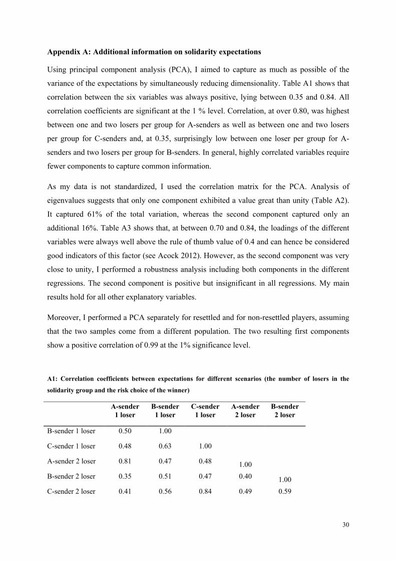
30
Appendix A: Additional information on solidarity expectations
Using principal component analysis (PCA), I aimed to capture as much as possible of the
variance of the expectations by simultaneously reducing dimensionality. Table A1 shows that
correlation between the six variables was always positive, lying between 0.35 and 0.84. All
correlation coefficients are significant at the 1 % level. Correlation, at over 0.80, was highest
between one and two losers per group for A-senders as well as between one and two losers
per group for C-senders and, at 0.35, surprisingly low between one loser per group for A-
senders and two losers per group for B-senders. In general, highly correlated variables require
fewer components to capture common information.
As my data is not standardized, I used the correlation matrix for the PCA. Analysis of
eigenvalues suggests that only one component exhibited a value great than unity (Table A2).
It captured 61% of the total variation, whereas the second component captured only an
additional 16%. Table A3 shows that, at between 0.70 and 0.84, the loadings of the different
variables were always well above the rule of thumb value of 0.4 and can hence be considered
good indicators of this factor (see Acock 2012). However, as the second component was very
close to unity, I performed a robustness analysis including both components in the different
regressions. The second component is positive but insignificant in all regressions. My main
results hold for all other explanatory variables.
Moreover, I performed a PCA separately for resettled and for non-resettled players, assuming
that the two samples come from a different population. The two resulting first components
show a positive correlation of 0.99 at the 1% significance level.
A1: Correlation coefficients between expectations for different scenarios (the number of losers in the
solidarity group and the risk choice of the winner)
A-sender 1 loser
B-sender 1 loser
C-sender 1 loser
A-sender 2 loser
B-sender 2 loser
B-sender 1 loser 0.50 1.00 C-sender 1 loser 0.48 0.63 1.00 A-sender 2 loser 0.81 0.47 0.48 1.00 B-sender 2 loser 0.35 0.51 0.47 0.40 1.00 C-sender 2 loser 0.41 0.56 0.84 0.49 0.59

31
A2: Information on the components derived by using PCA for solidarity expectations
Eigenvalue Difference Proportion Cumulative
Component 1 3.67 2.70 0.61 0.61
Component 2 0.97 0.39 0.16 0.77
Component 3 0.58 0.10 0.09 0.86
Component 4 0.47 0.28 0.07 0.94
Component 5 0.19 0.07 0.03 0.98
Component 6 0.12 - 0.02 100
A3: Loadings of component 1 from the PCA
A-sender 1 loser
B-sender 1 loser
C-sender 1 loser
A-sender 2 loser
B-sender 2 loser
C-sender 2 loser
Loadings 0.75 0.78 0.84 0.77 0.70 0.83

“DANCING EVERY DAY”: LAND ALLOCATION AND SUBJECTIVE ECONOMIC
WELL-BEING IN CAMBODIA
SIMONE GOBIEN
Institute for Co-operation in Developing Countries, University of Marburg,
Am Plan 2, 35037 Marburg, Germany
Phone: +49 6421 2823736, Fax : +49 6421 2828912
correspondence to: [email protected]
Abstract
This paper analyzes the short-term effect of access to land on subjective economic well-being
in Cambodia. It compares the subjective economic well-being of non-resettled beneficiaries of
a land allocation project, voluntarily resettled beneficiaries of the same project, and a control
group of land-poor people living in the same area. Two factors, own landholdings and being
able to use the land for agricultural production, were found to have positively significant
effects for all three groups. These effects remained robust after controlling for income,
implying that non-income aspects such as improved future economic prospects and increased
economic stability play a role in subjective economic well-being. Hence, even if economic
gains measured in terms of income take some time to realize after a pro-poor land
distribution, subjective measures already show relevant improvements in the short term.
JEL Codes: D60, I32, I38, Q15
Keywords: Land distribution, Voluntary resettlement; Project evaluation, Subjective
economic well-being, Cambodia
Acknowledgements: I thank the Deutsche Gesellschaft für Internationale Zusammenarbeit and the LASED project team of IP/Gopa in Kratie, especially Franz-Volker Müller, Karl Gerner, Pen Chhun Hak, Phat Phalit, Siv Kong, Sok Lina, and Uch Sopheap, for the opportunity to do research in the LASED project and for financial, organizational, and logistical support, and Hort Sreynit, Soun Phara, and the team of research assistants for excellent support in the field. My special thanks go to Michael Kirk for comprehensive support and valuable comments and to Thomas Dufhues, Thomas Falk, Tom Gobien, Bernd Hayo, Christian Traxler, Susanne Väth, the participants of the World Bank Conference on Land and Poverty 2013, and the participants of the Brown Bag Seminar in Marburg for valuable comments.

2
1. Introduction
Providing secure access to land is a key policy for poverty reduction in rural areas where the
majority of the population depends on agriculture (Besley and Burgess, 2000; Finan et al., 2005;
Holden et al., 2011). Some possible economic benefits of secure access to land are: the
opportunity to earn income (Bouis and Haddad, 1990; Carter and May, 1999; Grootaert et al.,
1997; Gunning et al., 2000; Scott, 2000), better access to the credit market (Feder, 1988),1 higher
incentives to invest (Besley, 1995; Brasselle et al., 2002; Carter and Olinto, 2003), shifts in
power relations and social status (Binswanger et al., 1995), and the safety net function of land
tenure (Deininger, 2003).
Most studies of what happens when people are given access to land concentrate on just one of
these benefits. Investigating subjective well-being, as a broad umbrella concept, is one way we
can capture all the effects together (Diener et al., 1999; Dolan et al., 2008). Frey and Stutzer
(2002) argue that measures of subjective well-being are a good proxy for utility, including
current circumstances, positional concerns, past experience, and expectations for the future, and
should be seen as complementary to objective approaches. An advantage of this approach is that
we can measure well-being directly, since it is the individuals themselves who are in the best
position to assess their personal well-being.
Subjective measures have been found to be sufficiently stable and to react to changes in life
circumstances (Dolan and White, 2007; Ehrhardt et al., 2000; Krueger and Schkade, 2008).
Furthermore, they show a reasonable correlation with objective measures (see for example
Oswald and Wu, 2010). A number of studies have related subjective measures to different
measures of poverty.2 Kingdon and Knight (2006), for example, argue that subjective well-being
encompasses objective poverty measures such as income poverty and capability poverty. Rojas
(2008) claims that subjective poverty is a broader concept than income poverty: he finds a
considerable mismatch between the two measures and argues for a more frequent use of
subjective measures. In addition, subjective measures can help to overcome the danger of 1 A number of studies do not find evidence that providing secure land titles results in better access to the credit market (see for example, Carter and Olinto, 2003; Place and Migot-Adholla, 1998). 2 Severe criticism of the use of subjective well-being data as a measure of poverty has been voiced by Sen (1984). He argues that the poor adapt to their situation and this can seriously alter their perception of unbearable circumstances. However, the absolute value of the well-being measure is less important in my study, since I compared groups of poor people of similar economic status.

3
paternalistic approaches to the poor as they put the individual’s own evaluation in the center and
thereby contribute to the discussion on appropriate project indicators (Becchetti et al., 2011).
Studies using subjective well-being to evaluate the impact of development projects are still rare
(among the few exceptions are Becchetti et al., 2011 and Becchetti and Costantino 2008, for
participation in a fair trade project, Becchetti and Conzo, 2013, for a micro-credit program, and
van Landeghem et al., 2013, and de Moura and da Silveira Bueno, 2013, for a land distribution
and a land title program). This is probably because, even though the multidimensional nature of
poverty is widely accepted, economic and monetary targets are predominantly used when
assessing development cooperation. The World Bank, for example, has recently announced two
goals to achieve by 2030: “End extreme poverty by decreasing the percentage of people living on
less than $1.25 a day to no more than 3%” and “Promote shared prosperity by fostering the
income growth of the bottom 40% for every country” (World Bank, 2014).
Therefore, narrowing the field of interest to subjective economic well-being as a core dimension
of overall well-being can be useful as it allows us to quantify people’s appreciation of
improvements (Becchetti et al., 2011).3 Moreover, it is easier to identify the effect of economic
variables when they are not overlaid by non-economic impacts: variables which are relevant for
non-economic well-being do not have to be considered, which reduces the danger of omitted
variable bias (Hayo and Seifert, 2003). By using subjective economic well-being it is thus
possible to concentrate on the economic dimension of aspects like for example the income
effects of social networks without having to control for intrinsic preferences towards network
membership. We can claim, therefore, that subjective economic well-being provides more direct
guidance to policymakers.
Drawing on these arguments, I carried out a study in Cambodia on subjective economic well-
being related to land access. I compared survey data from three groups: non-resettled
beneficiaries of a land allocation project, voluntarily resettled beneficiaries of the same project,
and a control group of landless or land-poor people living in the same area. All the project
households received agricultural land, but while the non-resettled group was still living in their
3 Here the underlying fundamental assumption is that the utility function is separable with respect to different dimensions of well-being (Hayo and Seifert, 2003). A number of studies find that the correlation between subjective economic well-being and subjective overall well-being is high but far from perfect (e.g. Hayo and Seifert, 2003; Rojas, 2006, 2008).

4
village of origin, the resettled group took part in a voluntary resettlement scheme and moved to a
newly established village. I took a short-term perspective, looking at the first year following the
land allocation when participants had to make large investments but their gains from agriculture
were still small, and thus the danger of project dropout was at its highest.
I found a positively significant correlation between land size and subjective economic well-being
for the whole sample and for each sub-group separately. In addition, individuals who managed to
realize their first agricultural income from their land within this short period showed evidence of
significantly higher subjective economic well-being. Both results hold after controlling for
income, showing that non-monetary economic rewards drive these results. Project participation
per se did not have a positive correlation with subjective economic well-being. A dummy for
non-resettled project participants turned out negative, whereas a dummy for resettled participants
remained insignificant.
A review of the literature revealed that the effect of land on subjective well-being has received
little attention. In a descriptive analysis of the subjective well-being of land recipients, share-
croppers and landless people in Bangladesh, Huq et al. (2007) found that the land recipients had
the highest scores, followed by the sharecroppers, while the landless respondents had the lowest
scores. The only paper I am aware of that uses multivariate analysis to quantify the effect of
landholdings is van Landeghem et al.’s Moldova study (2013), which found a positive subjective
well-being effect for land distributed in a land reform, but a negative effect for the average
landholdings of neighboring households. This confirms other findings on relative income
showing that households judge their own situation by comparing it with others (Clark and
Oswald, 1996; Dedehouanou et al., 2013; Fafchamps and Shilpi, 2008; Ferrer-i-Carbonell, 2005;
Graham and Pettinato, 2002). Regarding secure property rights to land, the evidence is similarly
scarce. A notable exception is the study by de Moura and da Silveira Bueno (2013) of a land-title
program for residential land in Brazil, which found that households with secure titles were more
likely to belong to a happier group.
In any case, none of these papers concentrates on subjective economic well-being, even though
the relationship between land and the economic domain of well-being seems intuitively stronger
than the relationship between land and other standard domains such as health, family or
community well-being. Furthermore, these studies do not take into account the use of land for

5
agricultural production. In many agrarian societies land remains agriculturally unused, for
reasons such as geographical obstacles like dense forest or difficult access, or lack of investment
capital, which acquires special importance in development projects directed at the poorest class.
The remainder of the paper is organized as follows. Section 2 gives background information on
the land allocation project in Cambodia and discusses the sample selection and ex-ante
differences between the groups, Section 3 explains the conceptual framework and hypothesis,
Section 4 describes the empirical analysis, Section 5 discusses determinants of land use, and
Section 6 concludes.
2. Background information
2.1. The LASED project
LASED (Land Allocation for Social and Economic Development) is a pilot project conducted by
the Royal Government of Cambodia, supported by the German Agency for International Co-
operation (Deutsche Gesellschaft für Internationale Zusammenarbeit – GIZ) and the World
Bank. Between one and three hectares of agricultural land are distributed to landless and land-
poor households. Households can apply for residential and agricultural land, only agricultural
land or only residential land. All residential land is in a newly founded village and all
agricultural land is close by. The land recipients are supported to start economic activities on the
allocated agricultural land. After five years of continuous use of the land, households can obtain
a formal title for their project land.4
The data for this study were collected in Kratie Province, where the project is most advanced.
Land was distributed to 525 households in this province in late 2008. Applicants had to be living
in one of the two project communes (Changkrang and Sambok in Chetborei District), be landless
or land-poor (having less than half a hectare), and be identified by the project staff and village
representatives as the neediest people in the communities. According to the project staff, all but 1
to 2% of eligible households applied. The project participants were therefore a very nearly
complete representation of the poor households in these two communes. All of them applied for
4 For simplicity, I nevertheless use the term ‘landownership’ when referring to project land.

6
both residential and agricultural land, implying that they were willing to move permanently to a
new village, but only 52% were successful (resettled project participants), while 44% obtained
only agricultural land (non-resettled project participants).5 Residential land was given only to all
those households which did not have residential land before the start of the project, otherwise
resettled and non-resettled households were similarly needy. The locations of the agricultural and
residential land plots were distributed by lottery to all project beneficiaries. Households with
only agricultural land had to commute from their villages to their agricultural plots.
2.2. The control group
I considered only geographically close communes (also in Kratie Province, Chetborei District)
for the control group, and to minimize observable differences I applied the following additional
criteria:
i) The control communes had applied for participation in the LASED project, thus showing
evidence of having land available for distribution, having demand for land, and being willing to
distribute land to the poor.
ii) The control and the project communes have a similar poverty index (proportion of poor to
non-poor households) in the “Identification of Poor Households Program”, referred to as
“IDPoor”, a national project that aims to implement a standardized procedure to identify poor
households throughout Cambodia (Ministry of Planning, Cambodia, 2006).
iii) The control and project communes have similar soil fertility (measured by the average rice
yield per hectare in the wet season recorded in the Ministry of Planning’s Commune Database,
2005).
iv) Since road infrastructure determines market access, information flow and mobility, the
control and project communes have a similar infrastructure index, measured according to the
commune’s kilometers of type 1 (all weather, hard surface) and type 2 (all weather, loose
surface) roads and the average distance from all villages to the closest type 1 or type 2 road.
5 The remaining 4% (20 households) received only residential land and are excluded from the analysis.

7
v) Since the distance from the Mekong River essentially determines economic life in rural
Cambodia (e.g. income from fishing, irrigation possibilities, transport), the control and project
communes show a similar distance from the Mekong.6
For Changkrang, Kou Loab was the best choice of control commune, and for Sambok it was
Thema Kreae.
2.3. Sample selection
I collected my data on subjective economic well-being in 2010, about two years after the start of
the project and about one year after the land had been distributed and beneficiaries with
residential land had moved to the new village. Time and money constraints obliged me to use a
proportionate stratified random sampling design in which proportions were based on the
allocation in the project group and sampling in the control group was adjusted. Approximately
35% of all the project households were from Changkrang and 65% from Sambok. This was
reflected in my sample, in which 33% of the project households were from Changkrang and 67%
from Sambok, and 35% and 65% of the control households were from the respective control
communes Kou Loab and Thema Kreae.
Stratification can improve the accuracy of empirical results by increasing estimation efficiency
through reducing standard errors (Cameron and Trivedi, 2009, p. 164). In the project group there
were two strata: the commune of origin (Changkrang or Sambok) and the type of land:
agricultural (non-resettled participants) or residential and agricultural (resettled participants). The
control group was chosen from a list of poor households from the IDPoor project, and there was
only one stratum, the commune, as these households did not receive land from the project. I
interviewed 200 households in total: 94 from the control group, 43 non-resettled households, and
63 resettled households (see Table 1). To control for different sampling probabilities, I used
probability weights that were proportional to the inverse probability of being sampled in all the
regressions. Moreover, I followed Cameron and Trivedi (2009, p. 165), who recommend the use
of finite population correction in small samples to account for sampling without replacement.
6 Data for criteria iv and v were constructed by the author using the geo-referenced database created by the Japan International Cooperation Agency, 2002, updated by the provincial Geographical Information System from the Department of Land Management in Kratie Province.

8
Table 1: Sample description in 2010
Project commune Non-resettled households Resettled households Control commune Control households
Changkrang 21 (119) 15 (65) Kou Loab 33 (303)
Sambok 22 (113) 48 (228) Thema Kreae 61 (285)
Total sample 43 (232) 63 (293) Total sample 94 (588)
The numbers in brackets give the size of the total population of poor households in these communes.
In 2008, before the start of the project, I collected socio-demographic household characteristics
for 189 of the households in my sample: 94 control households, 48 non-resettled project
households, and 47 resettled project households. I collected data on subjective economic well-
being only in 2010.
2.4. Ex-ante differences in the sample
The control group was chosen to minimize differences between project and non-project
households. Data from the IDPoor program is the most comprehensive collection of information
on poor households in Cambodia, with a participatory process on several levels. Using this data
reduced the likelihood of missing out relevant households in my basic population of poor
households, and also the likelihood that a household from this list was isolated from relevant
village information such as the chance to participate in a development project.
Despite the random nature of my data, I did observe some differences between the groups in
2008 before land distribution (see Table 2). In the control group, household size was
significantly smaller than in the other two groups, whereas the dependency ratio was lowest in
the group of non-resettled households. However, I found no significant differences in terms of
income and credit, nutrient provision, and social indicators. Tests for differences in asset
endowment did not show relevant differences. Most importantly, the groups had owned similar
amounts of land before the land allocation and gained a similar proportion of their income from
agricultural production, and all the control households would have been eligible for the project.

9
Table 2: Characteristics of project and control households in 2008 before land distribution
Control group N= 94
Non-resettled N= 48
Resettled N= 47
Difference in
VARIABLES Mean Std dev
Mean Std dev
Mean Std dev
means+
General household characteristics Number of household members 4.744 2.218 5.488 1.925 6.070 2.729 a**, b*** Dependency ratio+++ 0.720 0.677 0.604 0.557 0.766 0.662 c* Age of household head 43.43 14.07 42.17 10.85 41.37 9.429 Income and credit Income per year 1,097 1,500 1,341 1,282 1,480 1,887 % of household income from agricultural production
14.845 22.757 18.697 21.4 13.725 18.935
Credit per year 214.0 240.9 192.8 242.1 169.0 226.6 Nutrition Number of days in previous week with reasonable food
2.734 2.608 2.390 2.509 3.209 2.965
Nutrient provision current year compared to previous year ++++
1.787 0.788 1.976 0.758 2 0.756
Assets Hectares of land before land distribution 0.281 0.489 0.272 0.575 0.286 0.645 Housing condition+++++ 4.127 1.272 4.365 1.299 4.302 1.186 Information technology++++++ 1.181 1.261 1.122 1.364 1.419 1.418 Mobility+++++++ 0.723 0.612 0.902 0.664 0.907 0.718 Social indicators Attendance of weddings 5.330 5.498 6.146 5.420 7.977 15.14 Pagoda visits per year 6.319 8.090 7.683 7.431 7.535 9.620 a= significant difference between control group and non-resettled project members, b= significant difference between control group and resettled project members, c= significant difference between non-resettled and resettled project members, *** p<0.01, ** p<0.05, * p<0.1 + Wilcoxon-Mann-Whitney, t-test, or test of proportions for difference in means ++ 1= female, 0= male +++ The household dependency ratio is defined as the number of dependent members (children younger than 12 or adults older than 65) over the number of independent members (individuals between 12 and 65). It is set to the maximum value in the sample for households without dependent members. ++++ 1= less food, 2= equal amount of food, 3= more food +++++ Index from [0,12] consisting of the sum of: material of roof: 1= thatch, palm leaves, plastic sheet, tarpaulin or other soft materials, 2= corrugated iron, 3= tiles, fibrous cement, or concrete; material of exterior walls: 1= saplings, bamboo, thatch, palm leaves, or other soft materials, 2= wood, sawn boards, plywood, corrugated iron, 3= cement, bricks, concrete; area of the floor: 1= 20 m2 or less, 2= 21–50 m2, 3= 51 m2 or more ++++++ 0= nothing, 1= radio, 2= stereo, 3= TV +++++++ 0= nothing, 1= bicycle, 2= motorbike ++++++++ 0= never/ less than once a year, 1= 1–4 times a year, 2= 5–8 times a year, 3= 9–12 times a year, 4= more often
10
3. Project participation, resettlement and land ownership in the context of economic well-
being
3.1. Project participation and voluntary resettlement
My sample was drawn from the very bottom of the income range in Cambodia and focus group
discussion revealed that these people feel extremely helpless and powerless. Using data from a
cross-country participatory poverty assessment, Narayan et al. (1999) show that poor people in
all the countries covered by the study frequently lack the power to control their own lives and
they say they have no hope for the future. This can change with participation in a land allocation
project. Land recipients in my sample expressed their delight in comments like: “Since we got
the land we are dancing every day” or “I finally see a future for my family – I know it will be
hard work but things will get better now”.7 As subjective well-being depends on not only the
current situation but also expectations for the future (Frey and Stutzer, 2002), the project
participants were likely to experience higher subjective economic well-being. On the other hand
one can argue that the project restricted their freedom of choice, and Narayan et al. (1999) find
that government support programs, though seen as important, are mostly experienced negatively.
The LASED project had two components: the distribution of agricultural land and the
distribution of residential land which goes along with voluntary resettlement. In my study all
households applied for both components such that a few other factors were likely to decrease the
subjective economic well-being of non-resettled beneficiaries. The disappointment at being
unsuccessful in their application for residential land and the inconvenience of having to commute
to their agricultural plots might reduce subjective economic well-being. Stutzer and Frey (2008)
found systematically lower subjective well-being for people who have to travel longer distances
to their workplace. A more serious cause of lower subjective economic well-being for the non-
resettled beneficiaries might be the lack of secure property rights (cf. de Moura and da Silveira
Bueno’s 2013 study, mentioned above). Since formal institutions are weak in Cambodia and land
rights are often not documented, the non-resettled households might not hold secure property
rights for their residential land, whereas the resettled beneficiaries could look forward to a secure
title after five years’ residence. Another possible cause of lower subjective economic well-being
for the non-resettled beneficiaries is that geographically scattered project participants are harder 7 Land recipients from the LASED project in 2010.
11
to reach. My data shows that project support was significantly lower for the non-resettled than
the resettled participants and that fewer of the non-resettled ones participated in training.
On the other hand, relocating causes stress. But economists explain migration at the micro level
in terms of an expected positive net return from cost-benefit calculations and therefore interpret
it as investment (Sjaastad, 1962). Most people make this decision expecting it will improve their
economic well-being, if only in the future (Nowok et al., 2013). The desire to improve one’s
status can also be a motivating factor in the decision to migrate (Lucas, 1997). Where
resettlement is voluntary, we can expect to see an increase in the migrant’s subjective economic
well-being if this improvements are achieved. But if expectations are not met, resettlement is
likely to be negatively related to subjective economic well-being. Kahneman et al. (2006) found
that economic gains from migration led to lower increases in subjective well-being than expected
and Nowok et al. (2013) found only temporary improvements. For the resettled beneficiaries,
opportunity costs – reduced time for farming because of having to build a new house, and
reduced income through loss of access to off-farm employment because of being distant from
their established social networks in their old villages – could decrease income and in turn
subjective economic well-being.
Economically driven migration can also have high social costs (Nowok et al., 2013) and through
this channel decrease subjective economic well-being. As distance is a major determinant of
social networks (Fafchamps and Gubert, 2007; Fafchamps and Lund, 2003), migrants run the
risk of losing these networks. Such networks constitute informal insurance against economic
shocks (Fafchamps, 2003; Townsend, 1994), so their loss is likely to decrease subjective
economic well-being. In support of this supposition, Gobien and Vollan (2013) have shown, in a
solidarity experiment in the same context as the present study, that willingness to help
anonymous fellow villagers was significantly lower in a resettled community than between non-
resettled land recipients in naturally established villages.
Taking all these arguments together, it was thus an open question whether I would find higher
subjective economic well-being for project participants (both resettled and non-resettled), so
empirical evidence was needed.

12
3.2. Landownership
According to the standard utility model, landownership should have a positive effect on
subjective well-being (van Landeghem et al., 2013). This includes an indirect effect coming from
changes in income due to land ownership. Even though some studies – such as McCulloch and
Baulch (2000), which simulates the distribution of two hectares of land to landpoor (owning less
than two hectares) or landless rural households in Pakistan, or Ravallion and Sen (1994), which
calculates the “upper bound of the real world outcome” of redistributive land reform in
Bangladesh – do not find that access to land has relevant positive effects on income, most
scholars agree that there is a positive association (see for example, Bouis and Haddad, 1990;
Grootaert et al., 1997; Carter and May, 1999; Gunning et al., 2000; Scott, 2000). Finan et al.
(2005) argue that there is a high but decreasing marginal return of land for endowments of less
than three hectares, which applies to the dataset in the present study.
But landownership can have additional effects on subjective economic well-being. In contrast to
income or consumption, which often show high volatility, land can be a long-term indicator of
economic well-being. It does not change easily and hence is easier to observe and to measure. It
is of great importance in the rural context and is identified as one of the core resources in rural
areas leading to material well-being (Bull et al., 2013; Narayan et al., 1999). Another advantage
of secure landownership is that it facilitates access to the credit market, as it can be used as
collateral for the lender (Feder, 1988). Becchetti and Conzo (2013) have shown that access to
credit has a positive effect on subjective well-being. They emphasize that the prospect of getting
credit in the future, which could in turn bring future economic benefits, plays a major role in
explaining higher subjective well-being. In addition, many studies have found that secure
landownership has a positive effect on investment (see for example Deininger and Chamorro,
2004; Goldstein and Udry, 2008), since it leads the landowner to expect increased future income,
and therefore is also likely to have an effect on subjective economic well-being.
Land tenure provides prestige and reduces social exclusion, and thereby shapes a person’s social
network (Deininger, 2003). It improves social status, which can lead to more friends, more
invitations to social events and better chances of finding a well-respected spouse (Binswanger et
al., 1995; van Landeghem et al., 2013). Townsend (1994) has shown that in India, where village
networks work as informal insurance in a context of weak formal institutions, landless villagers

13
have poorer access to these networks than those with land. Land increases security by enabling a
person to self-insure against shocks and providing access to the financial market, and creates
stability by giving a home and employment to future generations. These social aspects of land
tenure translate into higher economic security and thus are likely to be positively correlated with
subjective economic well-being.
Lastly, owning land can inspire strong attachment (Hamilton and Fischer, 2003) which might be
translated into higher subjective economic well-being when people farm their own property.8
Family labor can be used productively, helping to diversify the household’s income portfolio
(Deininger and Chamorro, 2004), reduce vulnerability, and increase food security. Key
informants interviewed in the present study agreed that the belief that landownership improves
your economic situation is very common in Cambodia.
The above arguments led me to propose the following hypothesis:
(H.1) Landownership has a positive effect on subjective economic well-being
However, since I examined only the short-term effects of a land distribution project, many of the
potential benefits might not have materialized at the time of the study. High costs of land
clearance, substantial opportunity costs, lack of material resources and insufficient family labor
might prevent the use of the land. Besides being a possible reason for lower household income,
unused land can cause feelings of shame because the household did not manage to take the
chance offered by the project and has proven less successful than other project members. This
again might influence the household’s economic prospects and decrease subjective economic
well-being.
Agricultural use of the land can be seen as an important life goal for farmers.
Lyubomirsky,Sheldon, and Schkade (2005) argue that intentionally chosen, “happiness-relevant”
activities which require some effort can improve subjective well-being. Other studies have also
found a positive relationship between subjective well-being and the pursuit of (important) goals,
or progress in achieving them (Kasser and Ryan, 1993; Sheldon et al., 2004).9 As the project
8 See Altman and Low (1992) for a discussion on different aspects of “place attachment”, including “possession attachment” (Belk, 1992). 9 Diener (2000) argues that only goals which are congruent with the person’s need increase happiness. Similarly, Kasser and Ryan (1993) distinguish between intrinsically and extrinsically motivated goals and say that only the

14
participants in this study had actively applied for land but only some were involved in productive
goal-directed activities on the land, higher subjective economic well-being for those people was
likely. I therefore proposed a second hypothesis:
(H.2) People who manage to make use of their land for agricultural production have higher
subjective economic well-being
4. Empirical analysis
4.1. The empirical model and variables
The underlying model has the following general form:
where is the dependent variable, represents a vector of information on household and
individual characteristics, includes land-related variables, in particular own landholdings,
relative landholdings and agricultural use of the land, is a vector of commune and village
specific variables, and refers to the error term. , and are vectors of parameters related to
the different variable categories.
The dependent variable measures subjective economic well-being on a scale from 0 to 10,
with the higher values representing higher subjective economic well-being. As the results of
ordinal and cardinal treatments of subjective well-being measures are very similar (Ferrer-i-
Carbonell and Frijters, 2004), I report ordinary least square (OLS) estimations in this paper.10
The main focus of the study was the influence of land on subjective economic well-being. I
therefore include the logarithm of household’s land size in each model. I also include a dummy
variable indicating whether the household has started agricultural production on the land. To
ensure that the main results hold for each sub-group, I start with this simple regression
specification separately for each group (see Table 6, regressions 1, 2, and 3). Thereafter, I use all
former work as a predictor of happiness. These distinctions are difficult to make in the context of extreme poverty and are not discussed further in this paper. 10 Using the Shapiro-Wilk normality test I cannot reject the null hypothesis that subjective economic well-being is normally distributed.

15
available observations and add a dummy for non-resettled project participants and a dummy for
resettled project participants to distinguish between the three groups (Table 6, regressions 4, 5,
and 6).
Regression 5 and 6 add additional control variables. Following van Landeghem et al. (2013), I
include the logarithm of relative land size in all further specifications (regressions 5 and 6 in
Table 6). People derive positive utility from having higher status than their peers because doing
better than others boosts their self-respect, because material and social benefits are related to
higher status, and because wealthier households are more secure since they have a better chance
of surviving in times of crisis (van Landeghem et al., 2013). Relative measures, mainly with
respect to income, are standard explanatory variables in the subjective well-being literature and
in most studies they are negatively correlated with subjective well-being measures (see for
example Clark and Oswald, 1996, for the UK; Ferrer-i-Carbonell, 2005, for Germany;
Fafchamps and Shilpi, 2008, for Nepal; Graham and Pettinato, 2002, for Russia and Peru;
Dedehouanou et al., 2013, for Senegal). But a number of studies find that relative concerns are
less important in low income settings (Akay, Martinsson and Medhin, 2012; Graham and
Pettinato, 2002; Kingdon and Knight, 2007; McBride, 2001) or even absent (Akay and
Martinsson, 2011) and Bookwalter and Dalenberg ( 2010) have even found that having richer
neighbors has a positive effect on poor individuals’ subjective well-being because of positive
community spillovers. With respect to land, van Landeghem et al. (2013) find a negative effect
of neighbor’s landholdings. They conclude that the relative component of landholdings is at least
as important as the absolute component.
Determining the appropriate reference group for relative concerns is difficult. Whereas most
authors use comparisons on the local level (e.g. village or community, see for example
Dedehouanou et al., 2013; van Landeghem et al., 2013), Graham and Pettinato (2002) find that
comparison on the national level is more relevant. Kingdon and Knight (2007) find opposing
effects for local and distant comparisons: close neighbors’ income had a positive effect on the
utility function whereas the income of people further away had a negative effect. Other authors
determine the reference group by age or race (Kingdon and Knight, 2007; Powdthavee, 2005)
whereas again others find intergenerational comparison more important than regional
(Bookwalter and Dalenberg, 2010).

16
With respect to migration, this question becomes even more challenging. Some studies use the
population at the place of destination as the reference group (e.g. Akay, Bargain and
Zimmermann, 2012), whereas Fafchamps and Shilpi (2008) find that migrants still compare their
relative standing to people living in their area of origin. Due to the short period since
resettlement, I use data from the commune of origin to construct relative landholdings. 11 I define
the relative landholdings of household i as the average landholdings of all people living in this
commune, excluding household i itself.
Age is often found to have a U-shaped relationship to subjective well-being (Blanchflower and
Oswald, 2008), hence I include the individual’s age and its square. The regressions also contain a
dummy variable measuring literacy. Dolan et al. (2008) say that the link between education and
subjective well-being is still unclear, since the identification is complicated by indirect effects
stemming from the correlation of education with health and income, and by unobserved
individual traits. Yet Hayo and Seifert (2003) find that, controlling for income effects, education
has a positive effect on subjective economic well-being. To understand the role of good health, I
include the number of days home due to illness during the last month, which is expected to be
negatively related to subjective economic well-being. I also control for gender effects. In studies
where gender is found to be significant, females tend to report higher subjective well-being
(Dolan et al., 2008; MacKerron, 2012).
Regression 6 in Table 6 also controls for the natural logarithm of household income and
household size. Income measures and also expenditure and consumption are likely to be
correlated with latent personality traits, health, past experience, and so on, and hence can lead to
spurious correlation with subjective well-being (DeNeve and Cooper, 1998; van Landeghem et
al., 2013). As no valid instrument for income is available, I follow van Landeghem et al. (2013)
and present estimations both excluding and including income measures. I also include the
poverty rate in the village of origin as a proxy for relative income, on the assumption that a
higher poverty rate goes along with lower average income.12 Again following Fafchamps and
Shilpi (2008), I use the village of origin as the reference for the whole sample, including the
resettled project participants, since I assume that relative income at origin is more important than
11 Data source: 2005 Commune Database. As landholdings are a long-term indicator, I do not expect major differences between landholdings in 2005 and at the time of my data collection. 12 Due to data limitations, it was not possible to construct neighbors’ average income.

17
at destination, due to the short period since resettlement and the relatively equal income
distribution in the resettled village induced by the selection criteria of the land allocation project.
Another group of control variables relates to the commune or village level. Infrastructure
variables (number of primary and secondary school classrooms in the commune, distance of the
village in km to the nearest type 1 or type 2 road, km of type 1 and type 2 road per commune,
and distance of the village from the district capital) are combined with measures related to land
productivity (rice production in the wet season per commune and the distance of the village from
the Mekong). Variables are either taken from the 2005 Commune Database or constructed by the
author. I use principal component analysis in order to reduce dimensionality, including the
component with the highest eigenvalue in regressions 5 and 6 in Table 6.
4.2. Descriptive analysis
Before looking at the regression results (Section 4.3 below), I present a descriptive analysis of
the data. The mean values for the dependent variable are presented in Table 3. Subjective
economic well-being is significantly higher for both project groups than for the control group,
and higher for resettled than for non-resettled beneficiaries.
Table 3: Descriptive analysis of subjective economic well-being
Control group N= 94
Non-resettled N= 41
Resettled N= 43
Difference in means+
VARIABLES Mean Std dev Mean Std dev Mean Std dev Subjective economic well-being 4.245 1.818 4.814 1.722 5.349 1.842 a**, b***, c*
a= significant difference between control group and non-resettled project members, b= significant difference
between control group and resettled project members, c= significant difference between non-resettled and resettled
project members, *** p<0.01, ** p<0.05, * p<0.1
+ t-test for difference in means
Average subjective economic well-being tends to increase with land size. As Table 4 shows,
average subjective economic well-being increases for households in the first to third land
quintiles but decreases slightly for those in the fourth quintile. The mean annual household

18
income shows a jump from the first to the second land quintile but only minor differences
between the second, third and fourth quintiles.
Table 4: Subjective economic well-being and household income per year according to land quintiles
1st land quintile N= 50
2nd land quintile N= 63
3rd land quintile N= 52
4th land quintile N= 35
VARIABLES Mean Std dev Mean Std dev Mean Std dev Mean Std dev Hectares of land 0.00214 0.00479 0.756 0.769 2.592 0.464 3.092 0.0345 Subjective economic well-being 3.740 1.747 4.746 1.616 5.327 1.978 5.143 1.751 Household income per year 491.6 554.1 1,162 1,589 1,140 979.7 1,300 1,102 + 1= less than others, 2= same as others, 3= more than others
Figure 1 shows the mean level of subjective economic well-being for all households with land in
the three groups (some households in the control group do not own land and are not considered),
divided into land users and non-users. In all three groups, average subjective economic well-
being is higher for those who use their land, and highest for the resettled beneficiaries.
Figure 1: Average subjective economic well-being according to use and non-use of land for production

19
Finally, Table 5 shows the household characteristics in 2010 after the land distribution. At that
time, considerable differences between the two groups existed. Household size still differs
significantly between project and control households, whereas it does not differ significantly
between resettled and non-resettled households. Landownership differs as expected between
control and project households, at the 1% significance level, and productive use of the land also
differs between control and project households at the 1% significance level even if only
landowners are considered. Average landholdings in the commune are also significantly larger in
both project groups than in the control group and again higher in the group of resettled project
members. And yearly household income is significantly lower in the control group but does not
differ between resettled and non-resettled households.
Table 5: Characteristics of project and control respondents in 2010 after land distribution
Control group N= 94
Non-resettled N= 41
Resettled N= 43
Difference in
VARIABLES Mean Std dev
Mean Std dev
Mean Std dev
Means+
General household characteristics Number of household members 5 2.337 5.651 1.926 5.587 2.107 a*, b* Household income per year 920.4 659.9 1,429 1,270 1,314 1,528 a***, b** Hectares of land 0.209 0.405 2.581 0.587 2.542 0.806 a***, b*** Landownership (1= yes, 0= no) 0.596 0.493 1 0 1 0 a***, b*** Land used for production, all households (1= yes, 0= no)
0.372 0.486 0.884 0.324 0.889 0.317 a***, b***
Land used for production, households with land (1= yes, 0= no)1
0.625 0.489 0.884 0.324 0.889 0.317 a***, b**
Relative landholdings 0.839 0.278 0.952 0.01 0.957 0.008 a***, b***, c***
Characteristics of the interviewee Gender, 1=f, 0=m 0.638 0.483 0.628 0.489 0.651 0.481 Age 43.06 13.45 42.88 11.17 38.59 11.20 b**, c** Ability to read and write 1.191 0.396 1.163 0.374 1.143 0.353 Health 2.798 5.940 7.535 10.31 2.302 6.150 a***, c*** a= significant difference between control group and non-resettled project members, b= significant difference between control group and resettled project members, c= significant difference between non-resettled and resettled project members, *** p<0.01, ** p<0.05, * p<0.1 + Wilcoxon-Mann-Whitney, t-test, or test of proportions for difference in means 1 In the control group, only the 56 households with land are considered.

20
Interviewees are significantly younger in the resettled group than in the non-resettled and control
groups. The number of days home due to illness during the previous four weeks is significantly
higher in the non-resettled group than in the resettled and control groups. This result is mainly
caused by outliers, as in all groups more than 50% did not stay at home due to illness.
4.3. Regression analysis
Table 6 shows regression results.13 Confirming hypothesis H.1, land size has a significant and
positive effect on subjective economic well-being in all model specifications. With a coefficient
between 0.118 and 0.165 on the logarithm of land in regressions 4 to 6, the effect is rather small.
In line with hypothesis H.2, the dummy for productive use of the land becomes positively
significant in all specifications involving the whole sample and, with a coefficient between 0.462
and 0.652 (regressions 4 to 6), adds more substantially to subjective economic well-being. It just
misses the 10% significance level in the control group (regression 1) but turns out positively
significant in the separate regressions for the two project groups (regressions 2 and 3).14 Relative
amount of land shows the expected negative sign in regressions 5 and 6. Confirming van
Landeghem et al. (2013), at -0.449 and -0.639 the effect is bigger than the coefficient on own
landholdings. But whereas in regression 5 a Wald test does reject the hypothesis that the
coefficient on own landholdings equals the negative coefficient on relative landholdings at the
5% significance level, the same test cannot be rejected for regression 6.
The coefficients on the logarithm of own land show only minor changes if we compare
regression 5, which excludes own and relative income measures, with regression 6, which
includes these terms (Wald tests for equality of coefficients cannot be rejected). The dummy for
productive use of the land, on the other hand, decreases significantly if we compare regressions 5
and 6 (p-value for a Wald test for equality of coefficients = 0.058). This shows that part of the
effect stems from higher income for households that use their land for agricultural production.
Nonetheless, the positive association between both main variables, land size and the dummy for
productive use, and subjective economic well-being remains significant in regression 6.
Therefore, channels other than increased income also seem to be relevant.
13 To test for multicollinearity, I calculate the variance inflation factor after a regression without survey correction including all control variables. As expected, age and age squared show high multicollinearity. All other control variables stay well below the rule of thumb value of 10. 14 Relative landholdings are not included in the separate regressions, as the variation within the groups is too small.

21
Table 6: OLS regressions for subjective economic well-being
VARIABLES (1) (2) (3) (4) (5) (6) Control
group Non-resettled
project participantsResettled project
participantsComplete
sampleComplete
sample Complete
sample Project dummy -0.530*** -0.567*** -0.506*** non-resettled (0.116) (0.128) (0.132) Project dummy -0.00403 -0.0451 -0.0403 resettled (0.111) (0.109) (0.109) Log land 0.194*** 0.501* 0.170*** 0.165*** 0.118*** 0.125*** (0.0263) (0.253) (0.0360) (0.0200) (0.0195) (0.0184) Dummy land used
0.269 0.870*** 0.899*** 0.522*** 0.652*** 0.462***
for production (0.165) (0.194) (0.188) (0.109) (0.0983) (0.100) Log relative land
-0.639*** -0.449*
(0.228) (0.230) Age -0.0114 -0.0290* (0.0155) (0.0153) Age squared 0.000143 0.000283* (0.000167) (0.000165) Literacy 0.765*** 0.559*** (0.103) (0.102) Gender (1= female)
0.0878 0.0943
(0.0835) (0.0812) Days of illness -0.0374*** -0.0387*** (0.00473) (0.00452) Village infrastructure
0.203*** 0.0965**
(0.0302) (0.0457) Log income 0.566*** (0.0580) Poverty rate in the
0.0134**
village of origin (0.00516) Household size -0.0397** (0.0187) Constant 4.971*** 3.608*** 4.413*** 4.755*** 4.178*** 0.877* (0.151) (0.226) (0.171) (0.107) (0.347) (0.476) Observations 94 43 63 200 200 200 R-squared 0.115 0.037 0.030 0.124 0.182 0.220 Standard errors in parentheses: *** p<0.01, ** p<0.05, * p<0.1
The non-resettled households show a lower subjective economic well-being than the control and
the resettled groups (regressions 4 to 6). The dummy for the resettled group does not turn out
significant. Regressions 5 and 6 reveal further a positively significant dummy for literacy and a
negatively significant effect of illness. Village infrastructure also seems to add positively to

22
subjective economic well-being. Adding own income and village poverty to the model
(regression 6) shows a positively significant coefficient for both variables, together with a
negatively significant coefficient for the number of household members.
4.4. Robustness tests
Table 7 presents a further robustness check based on the specification in regression 6 of Table
6.15 To test the impact of the estimation procedure, I start by using ordered logit specifications in
regression 1 of Table 7. The logistic estimations are consistent with the OLS estimations for the
main variables of interest as they show positively significant coefficients for own landholdings
and land used for production. In addition, the dummy for non-resettled project participants again
turns out negatively significant and the dummy for resettled participants insignificant. Relative
land size is less stable: it is insignificant and positive in the ordered logistic estimation.
Secondly, I test an alternative specification for productive use of the land. In regression 2 of
Table 7, I include the natural logarithm of agricultural income in the model. Land size and the
dummy for non-resettled project members enter significantly and with similar size in the
regression. The coefficient of total household income remains positively significant, with a small
decrease in magnitude which lies within the 95% confidence interval of regression 6 in Table 6.
Agricultural income enters significantly with a small positive coefficient. This confirms that
additional utility is derived from productive use of the land, beyond just the income effect.
Thirdly, to check whether outliers drive my results, I calculate Cook’s distance after an OLS
regression without survey correction. I find that 11 observations show a value higher than the
rule of thumb of 4/n. In regression 3 of Table 7, I estimate the regression with a survey
correction excluding these influential observations. The results for the two main variables remain
significant and similar in size.
Fourthly, I test for the sensitivity of my results to the survey correction by using an OLS
estimation with robust standard errors and controlling for sampling weight in regression 4 of
Table 7. Influential observations are again excluded. As expected, standard errors increase. Own
landholdings remain robust on the 10% significance level and the dummy for productive use of
the land just misses the 10% level (p= 0.100). 15 The main results hold also for the specifications in regressions 4 and 5 of Table 6.

23
Table 7: Robustness analysis for the regressions on subjective economic well-being
(1) (2) (3) (4) (5) VARIABLES Ordered logit
estimation with survey correction
OLS with survey
correction
OLS with survey correction
OLS with robust standard errors
OLS with survey correction
Project dummy non-resettled
-0.387** -0.554*** -0.368*** -0.363
(0.155) (0.131) (0.118) (0.419) Project dummy resettled
-0.0719 -0.0458 -0.131 -0.137
(0.127) (0.110) (0.103) (0.363) Log land 0.117*** 0.148*** 0.108*** 0.109* 0.137*** (0.0221) (0.0166) (0.0174) (0.0639) (0.0175) Dummy land used for
0.599*** 0.524*** 0.535 0.570***
Production (0.123) (0.0916) (0.324) (0.0960) Log agricultural income
0.0266***
(0.00645)Log relative land 0.110 -0.511** 0.369* 0.385 (0.266) (0.229) (0.199) (0.720) Age -0.0569*** -0.0240 -0.0386*** -0.0426 -0.0482*** (0.0164) (0.0155) (0.0138) (0.0499) (0.0167) Age squared 0.000567*** 0.000243 0.000415*** 0.000453 0.000527*** (0.000179) (0.000167) (0.000149) (0.000540) (0.000180) Literacy 0.811*** 0.551*** 0.636*** 0.638** 0.567*** (0.107) (0.101) (0.0734) (0.267) (0.104) Gender (1= female)
0.0668 0.102 -0.0114 -0.00356 0.0204
(0.0939) (0.0811) (0.0753) (0.264) (0.0801)Days of illness -0.0468*** -0.0366*** -0.0395*** -0.0394*** -0.0397*** (0.00521) (0.00449) (0.00341) (0.0116) (0.00427) Village infrastructure
-0.0431 0.111** -0.0217 -0.0306
(0.0517) (0.0452) (0.0393) (0.138) Log income 0.572*** 0.541*** 0.490*** 0.484** 0.455*** (0.0722) (0.0598) (0.0549) (0.193) (0.0566) Poverty rate in the village of
0.0265*** 0.0118** 0.0107** 0.0120
Origin (0.00663) (0.00512) (0.00485) (0.0181) Household size -0.0411* -0.0408** -0.0318* -0.0325 -0.0373** (0.0225) (0.0186) (0.0161) (0.0584) (0.0180) Village fixed effects
No No No No Yes
Constant 1.296*** 1.594*** 1.676 2.419*** (0.488) (0.435) (1.542) (0.462) Observations 200 200 189 189 200 R-squared 0.219 0.226 0.227 0.305 Standard errors in parentheses: *** p<0.01, ** p<0.05, * p<0.1

24
Finally, I include village fixed effects in regression 5 of Table 7.16 This specification does not
enable me to identify a coefficient for resettlement, as all the resettled project households live in
the same village. Moreover, I have to exclude village and commune control variables due to
multicollinearity. The main variables remain significant and do not show major changes in
magnitude.
5. Determinants of land use
Table 8 shows a logistic regression explaining the determinants of productive use of the land for
all household with access to land (N= 162, with 56 households belonging to the control group).
These results should be treated with caution, in particular as omitted variables might bias my
results. It seems that the resettled households are more likely to use their land for agriculture than
the two other groups, whereas the dummy for non-resettled project households does not turn out
significant. This higher probability for the resettled households can be explained by their better
access to their agricultural land, because they live near it, and by high support from the project.
And, unlike the control group, all project households receive considerable monetary and
technical support from the project, but the resettled households receive more support: in 2010
project transfers constituted on average 33.5% of their annual income, while for the non-resettled
households it was only 18%.
Land size shows a positive correlation with productive use. In addition, it seems to be important
if project households had land before the land distribution, suggesting that previous experience in
agriculture is a significant predictor of later land use. Furthermore, I find an inverted u-shaped
relationship for the age of the household head, and a positive influence of family labor and a
negative influence of household head’s illness on the probability of land use. Owning livestock
and having access to more efficient tools also increase the probability of land use.
16 Seventeen dummies are included in the regression. Results on the dummy variables can be obtained from the author.

25
Table8: Logistic regression for the dummy variable “land used for production” (marginal effects)
(1) VARIABLES Logistic regression
with survey correction
Project dummy non-resettled -0.0204 (0.0277) Project dummy resettled 0.0473* (0.0245) Land size 0.0256** (0.0113)Dummy for land additional to project land 0.0977*** (0.0142) Age of household head 0.00533* (0.00281) Age squared of household head -5.03e-05* (2.81e-05) Family labor 0.137*** (0.0373) Gender of head of household (1= female) 0.00899 (0.0134) Head of household is ill -0.0978*** (0.0355) Livestock 0.104*** (0.0123) Tools used for farming 0.111*** (0.0118) Observations 162 Standard errors in parentheses: *** p<0.01, ** p<0.05, * p<0.1
6. Discussion and concluding remarks
Land scarcity is a tremendous problem all over the developing world, where most people depend
on subsistence agriculture. Providing access to land is therefore key to reducing poverty. It offers
land recipients multiple benefits. To measure the total effect of these benefits, I compared
beneficiaries of a land distribution project in Cambodia with a control group, using subjective
economic well-being as the measure of reference. Subjective indicators enable us to quantify
people’s appreciation of changes. They put the individual at the center and help to overcome
paternalistic approaches towards the poor. Measures of subjective economic well-being can
provide more direct guidance to policymakers, as they take into consideration the fact that the
goals of development cooperation are often monetary. A further advantage is that economic

26
influences are not overlaid by non-economic aspects and omitted variable bias is less of a
problem.
My study sample consists of non-resettled beneficiaries who received agricultural land, resettled
beneficiaries who received both agricultural land and residential land in a newly founded village,
and a control group of similar households from adjacent areas. The three groups were very
similar before the land distribution. Land recipients started to make use of their land about one
year before my data collection but not all the beneficiaries had started agricultural production. At
this point there was considerable danger of project dropout, as investment needs were high but
income gains had not yet materialized.
Controlling for relevant socio-economic characteristics, I identified a positive link between land
size and subjective economic well-being for the whole sample as well as for all sub-groups
separately. I found significantly higher subjective economic well-being for those who had
managed to use their land for agricultural production. These effects remained robust after
controlling for income, implying that both own landholdings and productive use of the land
increase subjective economic well-being, beyond the effect of increased income. Non-income
effects of secure landholdings, such as improved access to credit and higher investment capacity,
improve people’s expectations of future economic conditions and thus affect their present
subjective economic well-being. Moreover, social aspects of land tenure, such as higher social
status, easier access to informal social networks, and greater income diversification, decrease
vulnerability and increase economic stability and thereby improve people’s subjective economic
well-being. Hence, even if economic gains measured in terms of income can take some time to
realize after pro-poor land distribution, subjective measures already show relevant improvement
in the short term.
When subjective well-being is seen as a proxy for utility (Frey and Stutzer, 2002), the causal
relationship goes clearly from behavioral variables like land use to subjective well-being. But a
number of studies argue for a bi-directional relationship (Frey and Stutzer, 2005; Lyubomirsky,
King, and Diener, 2005). Lyubomirsky, King, and Diener (2005) offer an extensive review of the
literature on the relationship between subjective well-being and success in various aspects of life.
They find evidence going in both directions. Therefore my results should be considered with
caution.

27
What remains to be ascertained in future research is whether these effects are permanent. Some
authors argue in favor of a “set-point” theory of subjective well-being (Brickman et al., 1978;
Campbell et al., 1976), which states that people’s subjective well-being is shaped by genetics and
personality traits and remains stable over their life time, and that deviations from this set-point
caused by major life events are only temporary. But a number of studies question this view, for
example Lucas et al. (2003), which finds a lasting effect for marriage, Lucas et al. (2004), which
finds lasting negative effects for unemployment, and Frederick and Loewenstein (1999), which
finds lasting effects for cosmetic surgery.
Improved long-term well-being could also come from increased income. Here adaptation seems
to be likely. In an early study, Easterlin (1974) demonstrated adjustment to higher income from
economic growth and argued that higher subjective well-being stems rather from relative
improvements. Leaving the economic domain, lasting effects of landownership seem more
likely. Easterlin (2005) sees only partial adjustment to non-economic domains such as family and
health. To some extent related is the research by Headey (2008, 2010), which finds that
prioritizing family related and altruistic goals has a lasting positive impact on subjective well-
being.
All this implies that people can actively improve their subjective well-being level even in the
long run. Nonetheless, external support through development projects can lead to substantial
benefits if people are assisted to start farming on their land. Deininger (2003) attributes the fact
that many land reforms, particularly in Latin America, have been unsuccessful to the failure to
provide land recipients with the necessary support to make use of it.

28
References
Akay, A., Bargain, O., Zimmermann, K.F., 2012. Relative concerns of rural-to-urban migrants in
China. Journal of Economic Behavior & Organization 81(2), 421–441.
Akay, A., Martinsson, P., 2011. Does relative income matter for the very poor? Evidence from
rural Ethiopia. Economics Letters 110(3), 213–215.
Akay, A., Martinsson, P., Medhin, H., 2012. Does positional concern matter in poor societies?
Evidence from a survey experiment in rural Ethiopia. World Development 40(2), 428–
435.
Altman, I., Low, S.M., 1992. Place Attachment. Plenum, New York.
Becchetti, L., Castriota, S., Solferino, N., 2011. Development projects and life satisfaction: an
impact study on fair trade handicraft producers. Journal of Happiness Studies 12(1), 115–
138.
Becchetti, L., Conzo, P., 2013. Credit access and life satisfaction: evaluating the nonmonetary
effects of micro finance. Applied Economics 45(9), 1201–1217.
Becchetti, L., Costantino, M., 2008. The effects of fair trade on affiliated producers: an impact
analysis on Kenyan farmers. World Development 36(5), 823–842.
Belk, R.W., 1992. Attachment to possessions. In: Altman, I., Low, S.M., 1992. Place
Attachment. Plenum, New York, pp. 37–62.
Besley, T., 1995. Property rights and investment incentives: theory and evidence from Ghana.
Journal of Political Economy 103(5), 903–937.
Besley, T., Burgess, R., 2000. Land reform, poverty reduction, and growth: evidence from India.
Quarterly Journal of Economics 115(2), 389–430.
Binswanger, H.P., Deininger, K., Feder, G., 1995. Power, distortions, revolt and reform in
agricultural land relations. Handbook of Development Economics 3, 2659–2772.

29
Blanchflower, D.G., Oswald, A.J., 2008. Is well-being U-shaped over the life cycle? Social
Science & Medicine 66(8), 1733–1749.
Bookwalter, J.T., Dalenberg, D.R., 2010. Relative to what or whom? The importance of norms
and relative standing to well-being in South Africa. World Development 38(3), 345–355.
Bouis, H.E., Haddad, L.J., 1990. Effects of agricultural commercialization on land tenure,
household resource allocation, and nutrition in the Philippines. Research report 79,
International Food Policy Research Institute (IFPRI), Washington, DC.
Brasselle, A.-S., Gaspart, F., Platteau, J.-P., 2002. Land tenure security and investment
incentives: puzzling evidence from Burkina Faso. Journal of Development Economics
67(2), 373–418.
Brickman, P., Coates, D., Janoff-Bulman, R., 1978. Lottery winners and accident victims: is
happiness relative? Journal of Personality and Social Psychology 36(8), 917.
Bull, T., Mittelmark, M.B., Kanyeka, N.E., 2013. Assets for well-being for women living in deep
poverty: through a salutogenic looking-glass. Critical Public Health 23(2), 160–173.
Cameron, A.C., Trivedi, P.K., 2009. Microeconometrics using Stata (Vol. 5). College Station,
Stata Press, TX.
Campbell, A., Converse, P.E., Rodgers, W.L., 1976. The Quality of American Life: Perceptions,
Evaluations, and Satisfactions (Vol. 3508). Russell Sage Foundation, New York.
Carter, M.R., May, J., 1999. Poverty, livelihood and class in rural South Africa. World
Development 27(1), 1–20.
Carter, M.R., Olinto, P., 2003. Getting institutions “right” for whom? Credit constraints and the
impact of property rights on the quantity and composition of investment. American
Journal of Agricultural Economics, 85(1), 173–186.
Clark, A.E., Oswald, A.J., 1996. Satisfaction and comparison income. Journal of Public
Economics 61(3), 359–381.

30
De Moura, M.J.S.B., da Silveira Bueno, R.D.L., 2013. Land title program in Brazil: are there any
changes to happiness? Journal of Socio-Economics 45(3), 196–203.
Dedehouanou, S.F.A., Swinnen, J., Maertens, M., 2013. Does contracting make farmers happy?
Evidence from Senegal. Review of Income and Wealth 59(2), 138–160.
Deininger, Klaus, 2003. Land Policies for Growth and Poverty Reduction: Key Issues and
Challenges Ahead. World Bank and Oxford University Press, Washington.
Deininger, K., Chamorro, J.S., 2004. Investment and equity effects of land regularisation: the
case of Nicaragua. Agricultural Economics 30(2), 101–116.
DeNeve, K.M., Cooper, H., 1998. The happy personality: a meta-analysis of 137 personality
traits and subjective well-being. Psychological Bulletin 124(2), 197.
Diener, E., 2000. Subjective well-being: the science of happiness and a proposal for a national
index. American Psychologist 55(1), 34.
Diener, E., Suh, E.M., Lucas, R.E., Smith, H.L., 1999. Subjective well-being: three decades of
progress. Psychological Bulletin 125(2), 276.
Dolan, P., Peasgood, T., White, M., 2008. Do we really know what makes us happy? A review of
the economic literature on the factors associated with subjective well-being. Journal of
Economic Psychology 29(1), 94–122.
Dolan, P., White, M.P., 2007. How can measures of subjective well-being be used to inform
public policy? Perspectives on Psychological Science 2(1), 71–85.
Easterlin, R.A., 1974. Does economic growth improve the human lot? Some empirical evidence.
In: David, P.A., Reder M.W. (Eds.), Nations and Households in Economic Growth.
Academic Press, New York, 89–125.
Easterlin, R.A., 2005. Building a better theory of well-being. In: Bruni, L., Porta, P.L. (Eds.),
Economics and Happiness: Framing the Analysis. Oxford University Press, Oxford.
Ehrhardt, J.J., Saris, W.E., Veenhoven, R., 2000. Stability of life-satisfaction over time. Journal
of Happiness Studies 1(2), 177–205.

31
Fafchamps, M., 2003. Rural Poverty, Risk and Development. Edward Elgar, Cheltenham.
Fafchamps, M., Gubert, F., 2007. Contingent loan repayment in the Philippines. Economic
Development & Cultural Change 55(4), 633–667.
Fafchamps, M., Lund, S., 2003. Risk-sharing networks in rural Philippines. Journal of
Development Economics 71(2), 261–287.
Fafchamps, M., Shilpi, F., 2008. Subjective welfare, isolation, and relative consumption. Journal
of Development Economics 86(1), 43–60.
Feder, G., 1988. Land policies and farm productivity in Thailand. Johns Hopkins University
Press, Baltimore.
Ferrer-i-Carbonell, A., 2005. Income and well-being: an empirical analysis of the comparison
income effect. Journal of Public Economics 89(5), 997–1019.
Ferrer-i-Carbonell, A., Frijters, P., 2004. How important is methodology for the estimates of the
determinants of happiness? Economic Journal 114(497), 641–659.
Finan, F., Sadoulet, E., de Janvry, A., 2005. Measuring the poverty reduction potential of land in
rural Mexico. Journal of Development Economics 77(1), 27–51.
Frederick, S., Loewenstein, G., 1999. Hedonic adaptation. In Kahneman, D., Diener, E.,
Schwarz, N. (Eds.), Well-being: The Foundations of Hedonic Psychology. Russell Sage
Foundation, New York, 302–329.
Frey, B.S., Stutzer, A., 2002. What can economists learn from happiness research? Journal of
Economic Literature 40(2), 402–435.
Frey, B.S., Stutzer, A., 2005. Happiness research: state and prospects. Review of Social
Economy 63(2), 207–228.
Gobien, S., Vollan, B., 2013. Playing with the social network: social cohesion in resettled and
non-resettled communities in Cambodia. MAGKS Papers on Economics 2013, Philipps-
Universität Marburg, Faculty of Business Administration and Economics, Department of
Economics (Volkswirtschaftliche Abteilung).

32
Goldstein, M., Udry, C., 2008. The profits of power: land rights and agricultural investment in
Ghana. Journal of Political Economy 116(6), 981–1022.
Graham, C., Pettinato, S., 2002. Frustrated achievers: winners, losers and subjective well-being
in new market economies. Journal of Development Studies 38(4), 100–140.
Grootaert, C., Kanbur, R., Oh, G.T., 1997. The dynamics of welfare gains and losses: an African
case study. Journal of Development Studies 33(5), 635–657.
Gunning, J. W., Hoddinott, J., Kinsey, B., Owens, T., 2000. Revisiting forever gained: income
dynamics in the resettlement areas of Zimbabwe, 1983–96. Journal of Development
Studies 36(6), 131–154.
Hamilton, S., Fischer, E.F., 2003. Non-traditional agricultural exports in highland Guatemala:
understandings of risk and perceptions of change. Latin American Research Review
38(3), 82–110.
Hayo, B., Seifert, W., 2003. Subjective economic well-being in Eastern Europe. Journal of
Economic Psychology (24), 329–348.
Headey, B., 2008. Life goals matter to happiness: a revision of set-point theory. Social Indicators
Research 86(2), 213–231.
Headey, B., 2010. The set point theory of well-being has serious flaws: on the eve of a scientific
revolution? Social Indicators Research 97(1), 7–21.
Holden, S.T., Deininger, K., Ghebru, H., 2011. Tenure insecurity, gender, low-cost land
certification and land rental market participation in Ethiopia. Journal of Development
Studies 47(1), 31–47.
Huq, M.M., Khan, A., Jahan, M.S., Haque, M.A., 2007. Effects of land ownership on
psychological well-being of the poor farmers of the northern parts of Bangladesh. Journal
of Life and Earth Science 2(2), 43–46.
Kahneman, D., Krueger, A.B., Schkade, D., Schwarz, N., Stone, A.A., 2006. Would you be
happier if you were richer? A focusing illusion. Science 312(5782), 1908–1910.

33
Kasser, T., Ryan, R.M., 1993. A dark side of the American dream: correlates of financial success
as a central life aspiration. Journal of Personality and Social Psychology 65(2), 410–422.
Kingdon, G.G., Knight, J., 2006. Subjective well-being poverty vs. income poverty and
capabilities poverty? Journal of Development Studies 42(7), 1199–1224.
Kingdon, G.G., Knight, J., 2007. Community, comparisons and subjective well-being in a
divided society. Journal of Economic Behavior & Organization 64(1), 69–90.
Krueger, A.B., Schkade, D.A., 2008. The reliability of subjective well-being measures. Journal
of Public Economics 92(8), 1833–1845.
Lucas, R.E.B., 1997. Internal migration in developing countries. In: Rosenzweig, M.R., Stark, O.
(Eds.), Handbook of Population and Family Economics. Elsevier Science, Amsterdam/
New York, 721–798.
Lucas, R.E., Clark, A.E., Georgellis, Y., Diener, E., 2003. Reexamining adaptation and the set
point model of happiness: reactions to changes in marital status. Journal of Personality
and Social Psychology 84(3), 527–539.
Lucas, R.E., Clark, A.E., Georgellis, Y., Diener, E., 2004. Unemployment alters the set point for
life satisfaction. Psychological Science 15(1), 8–13.
Lyubomirsky, S., King, L., Diener, E., 2005. The benefits of frequent positive affect: does
happiness lead to success? Psychological Bulletin 131(6), 803.
Lyubomirsky, S., Sheldon, K.M., Schkade, D., 2005. Pursuing happiness: the architecture of
sustainable change. Review of General Psychology 9(2), 111–131.
MacKerron, G., 2012. Happiness economics from 35,000 feet. Journal of Economic Surveys
26(4), 705–735.
McBride, M., 2001. Relative-income effects on subjective well-being in the cross-section.
Journal of Economic Behavior & Organization 45(3), 251–278.
McCulloch, N., Baulch, B., 2000. Simulating the impact of policy upon chronic and transitory
poverty in rural Pakistan. Journal of Development Studies 36(6), 100–130.

34
Ministry of Planning, Cambodia, 2006. Identification of Poor Households Programme (IDPoor).
http://www.mop.gov.kh/Projects/IDPoor/tabid/154/Default.aspx (accessed 09.01.2014).
Narayan, D., Chambers, R., Shah, M.K., Petesch, P., 1999. Global synthesis: consultations with
the poor. World Bank, mimeo, 22–23.
Nowok, B., van Ham, M., Findlay, A.M., Gayle, V., 2013. Does migration make you happy? A
longitudinal study of internal migration and subjective well-being. Environment and
Planning A, 45(4), 986–1002.
Oswald, A.J., Wu, S., 2010. Objective confirmation of subjective measures of human well-being:
evidence from the USA. Science 327(5965), 576–579.
Place, F., Migot-Adholla, S.E., 1998. The economic effects of land registration on smallholder
farms in Kenya: evidence from Nyeri and Kakamega districts. Land Economics 74(3),
360–373.
Powdthavee, N., 2005. Unhappiness and crime: evidence from South Africa. Economica,
72(287), 531–547.
Ravallion, M., Sen, B., 1994. Impacts on rural poverty of land-based targeting: further results for
Bangladesh. World Development 22(6), 823–838.
Rojas, M., 2006. Life satisfaction and satisfaction in domains of life: is it a simple relationship?
Journal of Happiness Studies 7(4), 467–497.
Rojas, M., 2008. Experienced poverty and income poverty in Mexico: A subjective well-being
approach. World Development 36(6), 1078–1093.
Royal Government of Cambodia 2003. Sub-decree no. 19 on Social Land Concessions.
http://www.cambodiainvestment.gov.kh/sub-decree-19-on-social-land-
concessions_030319.html (accessed 16.01.2014).
Scott, C.D., 2000. Mixed fortunes: a study of poverty mobility among small farm households in
Chile, 1968–86. Journal of Development Studies 36(6), 155–180.

35
Sen, A., 1984. Rights and Capabilities. In: Sen, A., Resources, Values and Development.
Blackwell, Oxford, 307–324.
Sheldon, K.M., Ryan, R.M., Deci, E.L., Kasser, T., 2004. The independent effects of goal
contents and motives on well-being: it’s both what you pursue and why you pursue it.
Personality and Social Psychology Bulletin 30(4), 475–486.
Sjaastad, L.A., 1962. The costs and returns of human migration. Journal of Political Economy
70(5), 80–93.
Stutzer, A., Frey, B.S., 2008. Stress that doesn’t pay: the commuting paradox. Scandinavian
Journal of Economics, 110(2), 339–366.
Townsend, R.M., 1994. Risk and insurance in village India. Econometrica 62(3), 539–591.
Van Landeghem, B., Swinnen, J., Vranken, L., 2013. Land and happiness. Eastern European
Economics 51(1), 61–85.
World Bank, 2014. What We Do. Available from: http://www.worldbank.org/en/about/what-we-
do (accessed 09.01.2014).

LIFE SATISFACTION, CONTRACT FARMING AND PROPERTY RIGHTS:
EVIDENCE FROM GHANA
SUSANNE JOHANNA VÄTH*, SIMONE GOBIEN and MICHAEL KIRK
Institute for Co-operation in Developing Countries, University of Marburg,
Am Plan 2, 35037 Marburg, Germany
Phone: +49 6421 2823736, Fax : +49 6421 2828912
*correspondence to: [email protected]
Abstract
Recently, large-scale land acquisition has increased dramatically in the developing world.
The question whether land deals can benefit both the local population and the investor is
therefore high on the international agenda. Contract farming is discussed as a possible
solution but studies identifying the causal effects are rare. Using data from a quasi-natural
experiment in contract allocation, we compare the subjective well-being of outgrowers and
independent farmers in the sphere of the biggest palm oil producer in Ghana. We identify a
positive causal effect of the outgrower scheme which increases subjective well-being by 1.5
points on a scale of 0 to 10. We find a substitutive relationship between having an outgrower
contract and having property rights, and thus we argue that by increasing security a contract
increases well-being, as secure rights to land matter substantially for the overall life
satisfaction of non-contract but not of contract farmers.
JEL Codes: D60, I31, Q13
Keywords: Contract farming, Property rights, Quasi-natural experiment, Subjective well-
being, Large-scale land acquisition
Acknowledgements: We would like to thank the following organizations for financial and/or logistic support for this research: the sector project ‘Land Policy and Land Management’ of the German Agency for International Co-operation (Deutsche Gesellschaft für Internationale Zusammenarbeit – GIZ) and the Ghana Market-oriented Agriculture Programme (MOAP), a joint programme of the Federal Republic of Germany, and the Ministry of Food and Agriculture of the Republic of Ghana. Our grateful thanks go also to the team of field assistants for data collection, Benjamin Kretzer for his support in data processing, and Fidele Dedehouanou, Tom Dufhues and Tom Gobien for their valuable comments on the paper. Any shortcomings are of course ours.

2
1. INTRODUCTION
Large-scale land acquisition, especially in Africa, is recently on the rise. Whether large-scale
investment in agricultural land promotes growth and development by increasing productivity,
providing infrastructure, improving technology, and creating work opportunities or whether it
harms the local population by exploiting the workers, causing environmental destruction, and
taking land away from local users is currently the subject of much debate in the literature
(Cotula et al., 2009; Görgen et al., 2009; Von Braun and Meinzen-Dick, 2009; Deininger et
al., 2011; Cotula, 2012; Deininger and Byerlee, 2012). Some authors argue that where a
country has a weak land governance system and at the same time a strong customary system,
as Ghana does, large-scale investors can acquire land through traditional authorities at the cost
of the local population (Schoneveld et al., 2011; Wisborg, 2012; Amanor, 2012).
Outgrower schemes1 could bring dual benefits in the sphere of large-scale investment in
agricultural land. Contracts, if they respect existing local land rights, could foster the
commercialization of farmers’ produce while at the same time enabling the investor to profit
from local land resources (Von Braun and Meinzen-Dick, 2009; De Schutter, 2011). Because
they are so prevalent in developing countries, especially in Africa, outgrower schemes
deserve particular attention (Grosh, 1994; Oya, 2012). In general, “contract farming” refers to
an agreement between a farmer and a firm which processes the farmer’s produce or puts it on
the market (Grosh, 1994). Institutional arrangements vary widely between different contracts.
De Schutter (2011) describes the optimal scheme as one which has reliable producers for the
investor, reliable buyers for the farmers and untouched secure land rights.2
Even though many studies identify positive effects of contract farming on the livelihood of
farmers, outgrower schemes are still controversial. On the positive side, several authors, for
example Porter and Phillips-Howard (1997), Warning and Key (2002), Bolwig et al., (2009),
Minten et al., (2009), and Bellemare (2012), identify income and productivity gains of
contract farming in Africa. Moreover, since contract farming can lead to risk-sharing between
the producer and the processor (Key and Runsten, 1999), it can reduce price and income
volatility (Minten et al., 2009; Bolwig et al., 2009), show positive spillover effects for non-
contract crops and for adjacent non-contract farmers (Warning and Key, 2002; Govereh and
Jayne, 2003; Minten et al., 2009; Bellemare, 2012), and reduce market imperfections by
1 We use the terms “contract farming” and “outgrower schemes” interchangeably. 2 For political discussions on the benefits of contract farming for poverty alleviation see also World Bank (2007) and UNCTAD (2009).

3
providing credit, inputs, technology and information and hence lower transaction costs
(Grosh, 1994; Key and Runsten, 1999; Deininger, 2011).
On the negative side, contract farming is interpreted as just a tool for the investor to extract
rents without positive effects for landowners (Little and Watts, 1994; Porter and Phillips-
Howard, 1997). Very unequal power relations can make producers more vulnerable, since
risks may be transferred to them and they may lose autonomy (Little and Watts, 1994; Porter
and Phillips-Howard, 1997; Key and Runsten, 1999). Moreover, the prevalence of contract
farming is found to disrupt social structures, disturb the local political ecology, increase
economic inequality, and increase workloads (Carney and Watts, 1990; Korovkin, 1992;
Dolan, 2001; Yaro and Tsikata, 2013).
Despite these negative findings, however, farmers seem generally very willing to enter into
contracts. Huddleston (2006) and Väth and Kirk (2014) have shown for our research setting
that contract offers were not refused and, similarly, Guo and Jolly (2009) find a large excess
demand for contract farming in China. Farmers’ main motive for signing a contract seems to
be to reduce uncertainty. Masakure and Henson (2005), for example, using principal
component analysis, show that reduced market uncertainty (a guaranteed market for crops, a
reliable supply of inputs, guaranteed minimum prices, and reliable transport provided to
collect the produce) is what drives farmers to produce under contract.3 In Ghana, it has been
found that farmers are eager to secure access to inputs, credit and extension services via an
outgrower scheme (Huddleston, 2006; Väth and Kirk, 2014). Guo and Jolly (2009) identify
market access and price stability as their main motives for entering into contracts. These
findings are supported by Blandon et al. (2009), who identify prearranged quantities and
prices as an incentive for farmers to sign contracts with supermarkets in Honduras. It
therefore seems that the big advantage of contracts is that they satisfy security needs.
In rural areas, a land tenure regime which guarantees secure property rights to land is another
way to satisfy these needs. By ensuring that future profits from investing in land return to the
landowner, these rights reduce uncertainty and help to overcome the inevitable time lag
between agricultural investment and output, and hence stimulate investment (Besley, 1995;
Brasselle et al., 2002; Carter and Olinto, 2003). Moreover, income gains (Bouis and Haddad,
1990; Grootaert et al., 1997; Carter and May, 1999; Scott, 2000; Gunning et al., 2000) and
3 Farmers in Schipmann and Qaim’s (2001) study in Thailand, on the other hand, did not show a preference for contract farming. Farmers were, however, more likely to choose a contract when input or credit provision was involved.

4
better social standing (Binswanger et al., 1995) for the holder of these rights ease the access
to credit (Feder, 1988)4 and open up social networks (Townsend, 1994), which in turn help to
smooth consumption patterns and improve food security (Deininger, 2003; Dekker, 2006).
To jointly capture all effects contract farming and its relation to secure property rights to land
we used a subjective well-being approach, which we understand as a measure of utility (Frey
and Stutzer, 2002). Since it comprises both monetary and non-monetary aspects, subjective
well-being is a good complement to more traditional approaches, which concentrate mainly
on monetary issues (Diener and Suh, 1997; Frey and Stutzer, 2002) and dominate the
literature on contract farming. Thus, by controlling for income effects, a subjective well-being
approach allows us to focus on risk-reducing mechanisms and security-related aspects, which
form a key dimension of subjective well-being (Oishi et al., 1999; Webb, 2009; Wills-Herrera
et al., 2011). In doing so, we go far beyond the direct monetary effects of contract farming.
Whereas some authors find high correlation between subjective well-being and objective
measures (Oswald and Wu, 2010), others argue that adaptation to circumstances and stable
dispositional characteristics lead to rather low correlations (Diener and Suh, 1997).
Identification of causal effects has therefore attracted considerable attention in the subjective
well-being literature (see Ferrer-i-Carbonell and Frijters, 2004, for a good overview on
estimation techniques).
We contribute to this literature by identifying the causal effect of contract farming on
subjective well-being in the sphere of a large-scale land acquisition. Unobserved differences
between contract and non-contract farmers, which are correlated with the outcome variable
(e.g. entrepreneurial spirit and ability, risk preferences, trust, or effort), make appropriate
estimation techniques necessary to avoid biased estimates. Several studies have used an
instrumental variable approach to correct for selection bias (e.g. Warning and Key, 2002;
Simmons et al., 2005; Miyata, 2009; Rao and Qaim, 2011; Bellemare, 2012). However,
Dedehouanou et al. (2013) claim that instruments are often weak. Using panel data on
contract farmers in Senegal, they find that having a contract had a positive influence on
subjective well-being.
Our study confirms the positive link between contract farming and subjective well-being for
oil palm farmers in Ghana. We take advantage of a research setting where contract allocation
took place as a quasi-natural experiment. Whereas using panel data can bias results because of 4 Some authors do not find improved access to the credit market from providing secure land titles (see for example Place and Migot-Adholla, 1998; Carter and Olinto, 2003).

5
omitted time-variant variables,5 natural experiments provide the most robust evidence of
causality (MacKerron, 2012). In addition, we broaden the view by using two measures of
contract farming, firstly a dummy variable indicating that a household has an outgrower
contract on at least one of its agricultural plots, and secondly by using the size of land under
outgrower contract. Both variables remain positively significant throughout different model
specifications. However, it seems that holding an outgrower contract, independently of the
size of land under contract, explains gains in subjective well-being better. Moreover, we
propose that contract farming contributes to subjective well-being by fulfilling security needs,
as property rights for land play an important role for non-contract holders but not for contract
holders. Hence, contract farming turns out to be a promising tool for overcoming lack of
security.
The remainder of the paper is structured as follows. In the next section, we discuss the
connection between contract farming and subjective well-being, and between secure property
rights to land and subjective well-being, and the way these two kinds of connection are
interlinked, with a special emphasis on security aspects. Section 3 describes our research
setting, including contract allocation as a quasi-natural experiment, Section 4 presents our
estimation strategy with a discussion of previous findings in the subjective well-being
literature, the data and descriptive statistics, as well as our empirical findings, and Section 5
concludes.
2. LIFE SATISFACTION AND THE SECURITY DIMENSION OF CONTRACT
FARMING AND PROPERTY RIGHTS
Overall life satisfaction can be understood as an aggregate concept which comprises various
domains (Meadow et al., 1992; Cummins, 1996; Van Praag et al., 2003; Rojas, 2007; Van
Praag and Ferrer-i-Carbonell, 2008). The identification and demarcation of different domains
is somewhat arbitrary (Rojas, 2008; Bardo and Yamashita, 2013), but over the last decade the
International Wellbeing Group (2013) has developed a standard “personal well-being index”
(PWI) which is widely used in developing and emerging countries (e.g. Tiliouine et al., 2006;
Webb, 2009; Wills-Herrera et al., 2011; Davey and Rato, 2012). The index identifies future
5 For example income movements and changes in well-being are linked through omitted variables such as “seniority in the workplace” (Gardner and Oswald, 2007).

6
security as an important feature of overall life satisfaction.6 Especially in developing
countries, where (rural) markets show high imperfections, formal safety nets are
underdeveloped, and stability needs are inadequately satisfied, security plays an important
role in overall life satisfaction (Oishi et al., 1999). Webb (2009) shows for Tibet that future
security is even slightly more important for overall life satisfaction than the standard of living
domain. Willis-Herrera et al. (2011) show from a different angle that perceptions of political,
economic and communitarian insecurity in turn have a negatively significant correlation with
subjective well-being in Columbia.
In the sphere of large-scale land acquisitions, contract farming is seen as one important way to
address security needs, as it reduces some of the risks a farmer has to face. Dedehouanou et
al. (2013) point out that marketing risk is reduced because there is a secure buyer for the
produce and improved access to the market, and production risk is reduced because inputs and
credit are provided by the contractor. However, they also mention that it brings one new risk:
a contract may be breached, either by the buyer, because of decreased demand for processing
or by the farmer, because of failure to meet high quality standards.
Apart from the security aspects, Dedehouanou et al. (2013) indicate that contract farmers may
earn higher income, have more self-esteem, be more efficient because they receive training,
and have better health conditions due to access to less harmful pesticides and other chemicals
– all benefits which increase subjective well-being. On the other hand, contract farmers lose
their autonomy and may have to adapt their production and management techniques to meet
specified quality standards (especially for export production), which can mean increased
pressure and higher labour requirements and consequently decreased subjective well-being. In
a setting with very unequal power relation, farmers are endangered to enter into adhesion
contracts which foster such negative effects. Therefore, Dedehouanou et al. (2013) argue that
contract farming can affect overall life satisfaction both positively and negatively. As in our
particular setting the risk of contract breach by the buyer is rather negligible due to the excess
demand for oil palm fruits, and as the contractual agreement does not specify particular
quality standards, we expect that positive effects will outweigh the negative ones. Thus, we
hypothesize that holding an outgrower contract has a positive influence on farmers’ subjective
well-being. In line with Masakure and Henson (2005), Guo and Jolly (2009), and Blandon,
Henson and Islam (2009), who highlight the reduction of uncertainty as the main motive for
6 Based on Cummins (1996), the PWI lists eight domains of life: standard of living, personal health, life achievement, personal relationships, personal safety, community connectedness, future security, and spirituality/ religion.

7
entering into contracts, we believe that security is the aspect most responsible for enhanced
overall life satisfaction, when controlling for income effects.
Secure property rights to land are a second important way to address the security needs of
rural households and thus increase their subjective well-being. In the absence of these rights,
land conflicts arise when an increasing demand for land meets a limited supply. This is
especially the case when a large-scale investor enters the scene and demands huge tracts of
land. Thus, numerous studies document land disputes around large-scale investments, mostly
to the disadvantage of the local population (Li, 2011; Borras Jr and Franco, 2012; German,
2013). Clearly defined property rights can foster social stability and prevent disputes (Palmer
1998) and are therefore a precondition for satisfying the needs of both the local population
and the investor.
Moreover, land with secure property rights can be used as collateral to access the credit
market (see for example the seminal work by Feder, 1988, in Thailand, which identifies the
credit supply effect as the main benefit from land titling). In particular, it allows the farmer to
enter the formal lending market, where imperfect information about the borrower and high
monitoring costs are even more of an obstacle than in the informal sector (Feder and Nishio,
1998). If households are credit constrained, any increase in investment may be accompanied
by decreased consumption in the short run. Access to credit in turn reduces food insecurity,
mitigates health shocks and decreases vulnerability to environmental disasters. Thus, in line
with Deininger (2003), we can say that secure property rights to land provide an important
safety net function which is expected to enhance subjective well-being.
In addition, secure ownership reduces the time spent on protecting property and allows
household members to spend it on other activities (Field, 2007). This may lead to greater
labour market participation, thus increasing non-agricultural income, which may lead to an
increase in subjective well-being beyond addressing security needs. Finally, secure property
rights guarantee the long-term use of the land and thereby increase investment incentives,
which may bring additional income and improve agricultural productivity (e.g. Deininger and
Chamorro, 2004; Deininger and Jin, 2006; Goldstein and Udry, 200; Fenske, 2011). Higher
income in turn is positively associated with subjective well-being.7 Consequently, we
hypothesize that holding secure property rights to land has a positive influence on farmers’
7 Compare Besley (1995) for a discussion on endogeneity issues, for example that investment may not be a response to higher levels of tenure security but rather undertaken to enhance tenure security.

8
subjective well-being. Again, we assume that this is mainly caused by gains in security when
controlling for income effects.
Considering that both holding an outgrower contract and possessing secure property rights are
expected to have a positive influence on the security domain and in turn overall life
satisfaction, it is worthwhile conceptualizing possible links. Whereas several researchers
assume an additive relationship between domain satisfaction and overall life satisfaction (e.g.
Møller and Saris, 2001; Van Praag and Ferrer-i-Carbonell, 2008), Rojas (2006) provides
theoretical and empirical evidence that a constant elasticity of substitution (CES) specification
is preferable. Thus, allowing a variety of imaginable relationships between domain
satisfaction and overall life satisfaction, he shows for Mexico that effects on overall life
satisfaction emanating from increasing satisfaction in one domain tend to decay with
increasing satisfaction in this domain. This is in line with Palmer’s diminishing marginal
returns argument (1998), which states that once a certain level of security has been reached,
the benefits of additional security will be too small to foster further efforts to realize extra
security. In the context of overall life satisfaction, we therefore assume a substitutive rather
than an additive relationship between contract farming and secure property rights to land.
3. RESEARCH SETTING
3.1. The Investor
Our research was conducted within a 30 km radius of the Ghana Oil Palm Development
Company (GOPDC) large-scale investment. GOPDC is the biggest palm oil producer in
Ghana. It was founded in 1976 as a state-owned company with 8,953 ha of land, expropriated
from the local population by the military government (Republic of Ghana, 1976; Sutton and
Kpentey, 2012). The land known as the Kwae Concession was gradually transformed into oil
palm plantations to feed the newly constructed large-scale mill. The investment is located in
the remote Kwaebibirem District in the Eastern Region, where the oil palm business was
introduced to facilitate local development (Huddleston, 2006; Huddleston and Tonts, 2007;
Fold, 2008; Fold and Whitfield, 2012; Adjei-Nsiah et al., 2012).
From 1986 onwards, an outgrower scheme was established through a World Bank supported
development programme which aimed to integrate the local population. At that time the mill
was not being used to anywhere near full capacity, because the expansion pace and yield of

9
the nucleus farm had been overestimated (World Bank, 1994; interviews with Lands
Commission senior official and GOPDC senior manager),8 so GOPDC was interested in
increasing the local supply.
In the course of the privatization wave in 1994, the government transferred GOPDC to the
Belgium investor Société d’Investissement pour l’Agriculture Tropicale (SIAT), which took
over the majority of shares (GOPDC, 2013; SIAT, 2013). In addition to the 50-years
leasehold for the Kwae Concession (as of 1976), GOPDC acquired 5,205 ha for the adjacent
Okumaning Concession (as of 2000) (Republic of Ghana, 2008; Sutton and Kpentey, 2012).
However, neither the concessions nor the outgrower scheme yielded enough oil palm fruit to
run the mill at full capacity (interview with GOPDC senior manager),9 so GOPDC
complements its nucleus-estate system with third party purchases from independent farmers.
Focus group discussions revealed that the local people have very mixed feelings about
GOPDC (Gyasi, 1994; Huddleston, 2006; Väth, 2013). On the one hand they complain about
the original expropriations by the military government in the 1970s, low wages, and problems
with daily operations, but on the other they are very grateful for the expansion of the oil palm
business in the area, the outgrower scheme, infrastructural developments, employment
creation, and corporate social responsibility (Huddleston, 2006; Huddleston and Tonts, 2007;
Väth, 2013). Thus it cannot yet be claimed that there is a stable relationship between the
investor and the local population.
3.2. Oil Palm Production Around the Large-Scale Investment
Besides a few large-scale producers, oil palm is typically grown by small- and medium-scale
farmers in Ghana. Investment costs for oil palm cultivation are high, and it is only a rational
choice for those who hold secure land use rights (property rights or long-term sharecropping
agreements), as the break-even point is not reached until the seventh year after planting (Poku
and Asante, 2008). Consequently, the poorest are excluded from any form of commercial oil
palm farming and we can conclude that all those farmers who cultivate oil palm hold secure
land use rights.
8 Semi-structured expert interviews were conducted in the Kwaebibirem District or Accra between October and November 2011 to enrich the quantitative database. To guarantee the anonymity of the interviewees, we reveal their (rough) position and organization but not their names. All interviewees were informed about the purpose of the study. Due to their reservation and the sensitiveness of the topic, interviews were not recorded. 9 For more details on GOPDC, please refer to Väth (2013).

10
There are two ways that the roughly 10,000 smallholder farmers in our research area can
cultivate oil palms: either independently or under contract. Roughly 3,000 households grow
them as fully independent farmers. They can choose whether to sell their produce to the local
market or to GOPDC (interview with Ministry of Food and Agriculture official). In contrast,
at the time of data collection, 7,279 outgrowers were obliged to deliver the fruit from a
contracted oil palm plot to GOPDC. Households typically cultivate more than one plot; hence
a farmer can be an outgrower on one plot and also grow oil palm or other crops as an
independent farmer on another non-contracted plot. In our sample more than 90% of
households holding an outgrower contract on one plot are at the same time growing oil palm
independently on other plots.
GOPDC and the local economy compete in their demand for oil palm fruit (Poku and Asante,
2008). GOPDC’s pricing, for both outgrowers and independent farmers, is based on
developments in the world market price for crude palm oil (GOPDC, n.d.; interviews with
GOPDC senior manager and outgrower association executives; focus group discussion with
farmers). GOPDC offers higher prices than the local market in the domestic peak season as
the Ghanaian supply is too small to have an impact on the world market. In contrast, the local
market pays more in the lean season when oil palm fruit is scarce and domestic demand is
high. In a weak institutional setting paired with high monitoring costs, outgrowers could
breach contracts and sell to local markets (Fold, 2008; Fold and Whitfield, 2012) without fear
of legal consequences.10 The competitive demand setting is therefore more advantageous for
oil palm farmers than a situation where monopolistic structures weaken the smallholders’
bargaining power. Output markets for GOPDC and small-scale processors are discrete.
Whereas the red cooking oil for local demand can technically be produced only by the small
mills, GOPDC produces the crude palm oil used by various industries (Osei-Amponsah et al.,
2012).
3.3. Contractual Treatment as Quasi-Natural Experiment
When it introduced the outgrower scheme, GOPDC did not follow a systematic strategy for
location and scope. Uneven performance and changing attitudes of different managements
created the framework for various expansion waves and their particular locations over the
years (interviews with GOPDC senior managers and outgrower association executives). To
10 To prevent side-selling, GOPDC improves its relations with the local population by enhancing its corporate social responsibility activities or increasing its prices. Since legal processes are expensive and slow in Ghana, legal action against breach of contract is not a workable solution to the problem (interviews with GOPDC senior managers).

11
minimize the transaction costs of extension activities and fruit collection, each phase of
expansion was bound to a strictly demarcated area with a one-shot offer to accept the contract
(interviews with GOPDC senior managers). Thus farmers were unable to predict the pace,
scope or sites of these expansions. Consequently, self-selection by strategic migration was
impossible in our research setting.
When GOPDC decided at a specific date to expand the scheme at a specific location, it
offered at short notice a 25-year contract for a specific plot to all farmers who were currently
holding a “ready-to-cultivate plot” with ownership rights (interviews with GOPDC senior
manager and outgrower association executives).11 Recognizing the domestic role of
sharecropping, at the same time GOPDC introduced a tripartite outgrower contract for
sharecroppers with 25-year land use rights.12 Apart from the fact that the landlord has to sign
the outgrower agreement, such tripartite contracts are indistinguishable from contracts with
farmers holding property rights to land (GOPDC, n.d.). Outgrowers receive extension
services, inputs and credit from the investor (GOPDC, n.d.). Corroborating the findings by
Huddleston (2006) and Fold (2008) that farmers were eager to enter into contracts to access
credit and technology, our interviews with the executives of the outgrower association and
focus group discussions with farmers revealed that to the best of their knowledge nobody had
ever rejected an offer.13
To prove ownership rights in rural Ghana is challenging as land administration is cumbersome
(Amanor, 1999). At the time of data collection, titles verifying property rights to land were
not available in the catchment area and deed registration was poor (interview with Lands
Commission senior official). But the predominantly customary land tenure system of the
Akyem proved to be dynamic as it invented a kind of “informal deed” (Gyasi, 1994; Amanor,
1999). Clan heads and chiefs began to document customary ownership rights and for a small
fee enabled land-owning farmers to participate in the scheme (interview with outgrower
11 A ready-to-cultivate plot is a cleared plot which is not cultivated with other food or cash crops, but ready to be newly planted. In our research area farmers typically cultivate various plots with food (maize, plantain, cocoyam, cassava, etc.) and cash crops (cacao, citrus, and oil palm) which can be partly intercropped (interview with Ministry of Food and Agriculture official). Given the different crop cycles over multiple farms as well as fallow periods, rural households commonly have ready-to-cultivate plots. 12 From the late 19th century, long-term sharecropping arrangements became more common than customary ownership rights in Akyem (Gyasi, 1994; Amanor, 1999; Amanor and Diderutuah, 2001). This was the result of increasing land pressure through population growth and the migration associated to the cocoa boom (Gyasi, 1994). Thus, as a flexible instrument to enhance the allocation efficiency of land and labour resources, sharecropping spread (Amanor and Diderutuah, 2001; Amanor, 2010). 13 To enrich the quantitative data, focus group discussions were conducted between September and November 2011 with independent farmers and outgrowers. Each group consisted of 7 to 15 participants of similar wealth level. They were held in the local languages Twi and Fante, and recorded and transcribed into English.

12
association executives; Amanor and Diderutuah, 2001). But even though the outgrower
scheme was established as a World Bank supported development project and contract farmers
received inputs and credit to cope with high investment costs, the poorest farmers are still
excluded from the oil palm business as they cannot provide the required land use rights (see
also Watts, 1994).
De facto, as many eligible farmers as possible were recruited for the project (Huddleston
2006; interview with GOPDC senior manager) since the investor strove to make full use of
the mill and the World Bank aimed to integrate the local population. Given the high cost and
the intention of expanding the scheme quickly, agronomic characteristics such as soil fertility
or rainfall patterns were not measured on the plots under consideration (interviews with
GOPDC senior managers). GOPDC’s staff only verified that plots were on low-lying land.
This assessment was rather pro-forma, as it is common knowledge in rural Ghana that low
land is more suitable than high for oil palm cultivation (Gyasi, 1994; Amanor and Diderutuah,
2001) and farmers do not cultivate oil palm on unsuitable land but rather enter into
sharecropping arrangements to balance their needs for low and high lands (Amanor and
Diderutuah, 2001). Moreover, to the best of our knowledge, GOPDC assessed neither
personal attitudes nor socio-economic characteristics.
De jure, additional criteria were introduced in the contract. Firstly, outgrower plots had to be
within 400 metres of an accessible road (GOPDC, n.d.). Recognizing that the road system in
the area was underdeveloped, either all farms had to be accessible or none, hence this
requirement was de facto not applicable (interviews with GOPDC senior managers and
outgrower association executives). Secondly, the outgrower contract called for participants
aged 18 to 45, but Huddleston’s data set (2006) shows that this criterion was not implemented
(which is also in line with statements made in interviews with GOPDC senior managers and
outgrower association executives).
To sum up: For oil palm farmers, both outgrowers and independent, secure land use rights
(i.e. property rights or long-term sharecropping arrangements) are indispensable and therefore
different performance cannot be the result of unequal access to documented land use rights.
Moreover, neither our treatment nor our control group (i.e. outgrower or independent farmers)
includes the poorest farmers, since high investment costs and difficult access to long-term
land use rights prevents them from cultivating oil palms commercially. Most importantly, it
was impossible to anticipate the location and scope of the scheme or the date when it would
be introduced, and no farmers rejected the scheme. Within the chosen area, both GOPDC and

13
the World Bank wanted to offer the contract to as many farmers as possible and de facto no
pre-selection of participating farmers took place. Hence, we treat the outgrower contracts as a
quasi-natural experiment.
4. EMPIRICAL ANALYSIS
4.1. The Empirical Model, Variables, and Estimation Strategy
We estimate the effect of the contractual treatment on subjective well-being using the
following general model:
yi stands for the dependent variable, xi is a vector of explanatory variables, including socio-
demographic variables of the respondents, li represents land related variables, most
importantly our measure of contract farming and property rights for land, ci includes
geographic information for the village and area, and refers to the error term. , and
are parameter vectors relating to the corresponding individual variables, land related variables
and geographic information respectively.
Our indicator for subjective well-being is overall life satisfaction, which runs from 0,
representing very low subjective well-being, to 10, representing very high subjective well-
being. We use ordinary least square estimations throughout our paper, following Ferrer-i-
Carbonell and Frijters (2004), who have shown that ordinal and cardinal treatment of the
dependent variables leads to similar results. Ordered logistic regressions are estimated as a
robustness check and can be found in Appendix B.
Our aim is to identify the causal effect of contract farming on subjective well-being in the
context of a large-scale land investment. We use two alternative measures for contract
farming. First, we include a dummy variable which takes on a value of one if a household has
an outgrower contract on any of its agricultural plots. Second, we replace the dummy by the
logarithm of land size under outgrower contract. The majority of households in our sample
cultivate several plots. Therefore, outgrowers may have some plots under contract and others
used independently. Using the dummy variable, we assume that contract farming has a
uniform effect on households independently of the size of land under contract. With our

14
second measure we relax this assumption by testing size effects assuming that a percentage
increase in the size of land under contract has a constant effect.
As having a contract may influence not only subjective well-being but also other household
characteristics such as income or aggregated assets, we start by estimating the net effect of
contract farming on subjective well-being by including only our measures for participation in
the outgrower scheme and exogenous socio-demographic characteristics (model 1 in Table 4
includes the dummy variable and model 2 in Table 4 the logarithm of land size under
outgrower contract).
In a second step, we include further land related controls in model 3 in Table 4, most
importantly the percentages of land with secure property rights, as well as additional socio-
demographic and wealth-related controls. We distinguish between two bundles of property
rights, to take into account the fact that customary land rights can vary in quality with regard
to disposal and mortgage. The first bundle comprises both the right to use the land as
collateral and the right to sell the land, whereas the second contains only the right to use the
land as collateral. Recalling that households typically cultivate more than one plot, we include
land with secure bundles of property rights as the percentages of the total amount of land
owned (running from 0 to 1). These are proxies for landownership at the household level
which allow us to capture different property rights regimes of different plots.
In model 4 we also include an interaction term between the bundles of property rights and the
outgrower dummy to identify heterogeneous effects for the treatment and the control group.
Even though we cannot know if the bundles of property rights to land are exogenous, the
interaction might give us a hint about the transmission channels of contract farming. In all
estimations we cluster the standard errors on the village level.
The socio-demographic control variables included in models 1 and 2 in Table 4 are age of the
head of household and its square, gender of the household head, a dummy variable indicating
whether the household does not belong to the regional ethnic majority (Akan), and a dummy
for households which migrated to the region before the start of the outgrower scheme. Many
studies find a u-shaped relationship between age and subjective well-being (e.g. Blanchflower
and Oswald, 2008), indicating lower levels of subjective well-being around middle age.
Studies on gender and subjective well-being find either no significant gender effects (Van
Landeghem et al., 2013) or higher average subjective well-being for females (Dolan et al.,
2008; MacKerron, 2012). Belonging to an ethnic minority or being a migrant show more

15
consistent results in the literature, with lower subjective well-being reported for these groups
(Verkuyten, 2008; Safi, 2010; Kirmanoğlu and Başlevent, 2013). Whereas some scholars
argue that the extent of assimilation to the host environment provides some explanation (Neto,
1995), others find that it is driven rather by perceived discrimination (Verkuyten, 2008; Safi,
2010).
Models 3 and 4 in Table 4 add additional controls. These include a dummy for marital status
of the respondent, because married people are believed to be more satisfied with life (Stack
and Eshleman, 1998; Diener et al., 2000),14 years of education, which are often found to be
correlated to subjective well-being, with results differing in terms of strength and direction
(Dolan et al., 2008), and a health variable (illness within the household during the previous
two weeks), because healthier people show higher subjective well-being (Dolan et al.,
2008).15
Income as a determinant of subjective well-being is the focus of a sizable number of research
papers. In general, they find a positive but diminishing correlation of income and subjective
well-being. However, reverse causality and further endogeneity problems, caused for example
by latent personality traits or uncontrolled health effects, make direct interpretation often
problematic. This is shown for example by Graham et al. (2004), using panel data from
Russia, who find that more satisfied people tend to have higher incomes. Therefore, some
studies instrument income with expenditure data (e.g. Kingdon and Knight, 2007; Asadullah
and Chaudhury, 2012; Van Landeghem et al., 2013). We decided to use data on household’s
self-rated surplus income, which we consider more relevant in the context of subjective
measures.16 This has the advantage of controlling at least partly for possible measurement
errors if we assume that measurement errors are correlated with each other over different
subjective measures. People’s understanding of what the levels on a scale mean can vary
considerably (Winkelmann and Winkelmann, 1998; Van Landeghem et al., 2013). For
example, a choice of 3 on a scale of 1 to 5 could indicate either a fairly high or a fairly low
level of well-being, depending on personal judgment. Moreover, people can show the same
14 Including marital status as a right-hand side variable raises issues of reverse causality. See for example Frey and Stutzer (2005) for a discussion. 15 Oswald and Powdthavee (2008), in their longitudinal study, find partial hedonic adaptation to becoming disabled. In line with this argument, Diener et al. (1999) argue for the use of subjective health measures. However, our results hold, as we include subjective health as an additional explanatory variable. 16 Question: Which of the following is true? The current income of the household: 1= Allows you to build your savings, 2= Allows you to save just a little, 3= Only just meets your expenses, 4= Is not sufficient, so you need to use your savings to meet expenses, 5= Is really not sufficient, so you need to borrow to meet your expenses. In addition we control for household size. We assume that sharecropping is captured by our control for household income. Nonetheless, our results hold as we include a sharecropping dummy.

16
average well-being levels despite different variance in well-being over time (Ravallion and
Lokshin, 2001).
We also use this proxy to construct a relative income variable. People tend to compare
themselves with their peer group, with two opposing effects at work (see Van Landeghem et
al., 2013, for the subsequent discussion). On the one hand, higher income of one’s peers can
be seen as a positive sign for overall development, hinting at future improvement of one’s
own situation, or it can lead to positive externalities, again improving one’s own situation; on
the other hand, having a higher income than one’s peers may lead to higher status,
incorporating material and social benefits and a better chance of survival in times of crisis.
Empirical research mostly finds the latter effect more pronounced, with negative correlation
between average peer’s income and subjective well-being (e.g. Dedehouanou et al., 2013, for
Senegal; Addai et al., 2013 for Ghana). We construct our measure of relative income of
household i as the average self-rated surplus income of all households living in the same
traditional area, excluding household i itself. Our data set includes households from three
traditional areas, Abuakwa, Kotoku, and Bosome. Anecdotal evidence supports our
assumption that people identify with their traditional group; however, results hold if we use
the village as the group identifier. In addition, we include an asset index as a stock variable
for household’s wealth. This variable can of course also be subject to endogeneity, further, it
might be correlated to household’s income. However, results hold for alternate use as well as
for including both variables and the variance inflation factor does not point to serious
multicollinearity.
Land related controls are the size of own and neighbours’ average agricultural land, the size
of the land under cultivation, and the duration of the outgrower contract. Again
multicollinearity is not a problem and results hold for alternative specifications. The effect of
landownership and secure access to land is seriously under-researched in the subjective well-
being literature even though land plays a key role in agrarian societies. In a study of a land
reform in Moldova, Van Landeghem, et al. (2013) find that own landholdings have a positive
effect on subjective well-being but that neighbours’ average landholdings have a negative
effect. Gobien (2014) has corroborated these findings in the context of a land distribution
project in Cambodia.

17
4.2. Data and Descriptive Analysis
Our survey was conducted between October and December 2010 within a 30 km radius of the
GOPDC oil palm mill. In total 824 household heads were interviewed – 436 outgrowers and
388 independent farmers. GOPDC permitted us to draw a random sample out of a total
outgrower population of 7,279. Choosing the 95% confidence level with a confidence interval
of 5, we ended up with 436 outgrowers spread over 47 different villages in the catchment area
(see Table 1).
In addition, we interviewed 388 independent farmers out of an estimated population of 3,000
households in a two-stage selection process (see Table 1). In a first step, we selected 25
villages out of these 47 villages by using village size (small, medium, large) as the stratum for
proportional sampling. In the small villages (< 1,000 inhabitants) we sampled all the
independent oil palm farmers, but we applied a second-stage cluster sampling for medium
(>1,000–5,000 inhabitants) and large (>5,000 inhabitants) villages. To avoid biases through
migration effects, we excluded from our survey migrant households which had been in the
catchment area less than 24 years since the introduction of the outgrower scheme.
Table 1. Populations and sampling
Contractual arrangement Population size Sample size
Outgrowers (OG) 7,279 436
Independent Farmers (IF) unknown ≈ 3,000 388
Observations ≈ 10,279 824
Note: OG are based on random sampling. IF are based on a two-stage sampling with community size as stratum and clustering at village level.
Tables 2 and 3 and Figure 1 offer some descriptive statistics for our sample. Table 2 shows
that mean life satisfaction for outgrowers (6.853) is significantly higher than for independent
farmers (5.345).
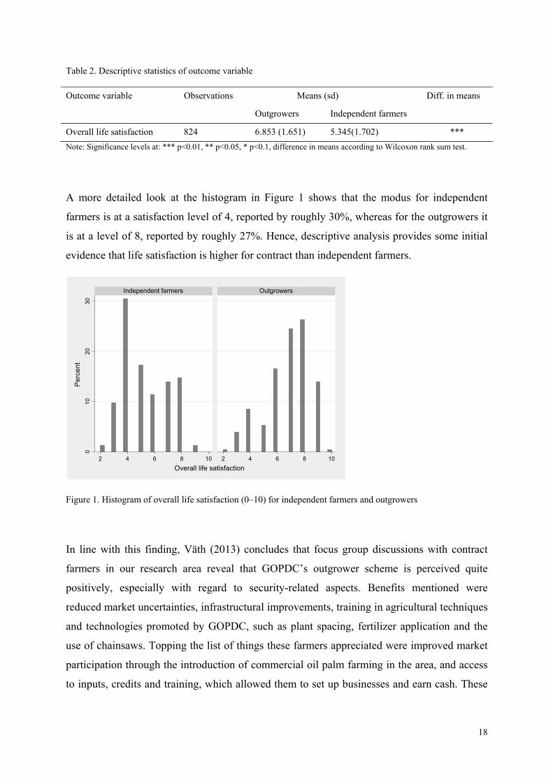
18
Table 2. Descriptive statistics of outcome variable
Outcome variable Observations Means (sd) Diff. in means
Outgrowers Independent farmers
Overall life satisfaction 824 6.853 (1.651) 5.345(1.702) *** Note: Significance levels at: *** p<0.01, ** p<0.05, * p<0.1, difference in means according to Wilcoxon rank sum test.
A more detailed look at the histogram in Figure 1 shows that the modus for independent
farmers is at a satisfaction level of 4, reported by roughly 30%, whereas for the outgrowers it
is at a level of 8, reported by roughly 27%. Hence, descriptive analysis provides some initial
evidence that life satisfaction is higher for contract than independent farmers.
Figure 1. Histogram of overall life satisfaction (0–10) for independent farmers and outgrowers
In line with this finding, Väth (2013) concludes that focus group discussions with contract
farmers in our research area reveal that GOPDC’s outgrower scheme is perceived quite
positively, especially with regard to security-related aspects. Benefits mentioned were
reduced market uncertainties, infrastructural improvements, training in agricultural techniques
and technologies promoted by GOPDC, such as plant spacing, fertilizer application and the
use of chainsaws. Topping the list of things these farmers appreciated were improved market
participation through the introduction of commercial oil palm farming in the area, and access
to inputs, credits and training, which allowed them to set up businesses and earn cash. These
010
2030
2 4 6 8 10 2 4 6 8 10
Independent farmers Outgrowers
Per
cent
Overall life satisfaction

19
benefits enabled them to enrol their children in school, and enabled some to save enough
money to send their children to university.
Table 3. Descriptive statistics of independent variables (means)
Means (sd) Diff. in CATEGORIES VARIABLES Outgrowers Independent farmers means (436) (388) Land-related Land under contract (in acres) 9.914 (7.625) - characteristics Own land (in acres) 6.202 (12.81) 4.821 (5.519) ** Land under cultivation (in acre) 17.27 (10.47) 9.410 (5.794) *** % of land with rights to sell and use
as collateral (0–1) 0.251 (0.364) 0.453 (0.460) ***
% of land with rights to use as collateral
0.0520 (0.186) 0.0880 (0.245) *
Socio- Education of household head (years)
8.25 (5.120) 6.938 (4.602) ***
demographic Gender of household head (1= female)
0.222 (0.416) 0.186 (0.389)
characteristics Age of household head 52.110 (11.243) 47.007 (12.56) *** Not Akan (different ethnicity) 0.374 (0.484) 0.353 (0.478) Migrant 0.314 (0.465) 0.139 (0.347) *** Household head is married 0.827 (0.380) 0.814 (0.389) Household member ill (last 2 w.) 0.408 (0.492) 0.183 (0.387) *** Household size 6.041 (2.844) 4.054 (2.09) *** Wealth Subjective income 3.278 (1.218) 3.317 (0.994) characteristics HH aggregated assets (in GH Cedi)+ 1,126 (24,274) 732 (3,673) *** Village level Large village (>5,000) 0.255 (0.436) 0.232 (0.423) characteristics Small village(>1,000) 0.294 (0.456) 0.289 (0.454) Traditional area: Bosome 0.0229 (0.150) 0.0387 (0.193) Traditional area: Kotoku 0.463 (0.499) 0.407 (0.492) Note: Significance levels at: *** p<0.01, ** p<0.05, * p<0.1; for dummies: yes = 1, no = 0; subjective income: 1= very high, 5= very low; two sample tests of proportions for dummies, otherwise Wilcoxon rank-sum tests are applied. +As assets are strongly skewed to the right, medians are more informative than means. The exchange rate for Ghana is at 1 October 2010: 1 GHS = 0.70 USD.
If we compare the independent variables in Table 3 we see that the two groups have quite
similar time-invariant socio-demographic and village level characteristics. However, asset
accumulation seems more prevalent for outgrowers than for independent farmers. Contractual
arrangements could have led the two groups on different development paths over the years. In
particular, contractors own more land and have more land under cultivation than the
independent farmers, and their aggregated assets are roughly one third higher. Independent
farmers depend more heavily on cash income for investment during the planting season and
have more need to accumulate savings to mitigate shocks than contract farmers do, since the

20
latter access inputs and credit through GOPDC. It seems likely that outgrowers use their cash
income to access and cultivate additional land and improve their livelihood by purchasing
new assets. In line with this idea, descriptive analysis reveals that outgrowers obtained
roughly 75% of their independently farmed food or cash crop plots after they entered into
contract farming. Thus, the “land gap” between outgrowers and independent farmers accrued
after contractual treatment.
4.3. Regression Analyses
As Table 4 shows, we find that holding an outgrower contract has a highly significant positive
effect in all four models. Confirming our hypothesis, the outgrower dummy has a strong
effect, increasing overall life satisfaction by roughly 1.5 points on a scale of 0 to 10 (models
1, 3 and 4). The size of the land under outgrower contract, however, has only a small effect.
The coefficient of 0.175 for the logarithm of contracted land in model 2 implies that a farmer
would need an increase in land under contract of over 30,000% to achieve a one point
increase in overall life satisfaction. It therefore seems likely that spillover effects of plots
under contract enhance life satisfaction for contract famers independently of the size of the
land under contract and that size-independent effects, like increased security or improved
access to credit, account for the major part of the effect. Consequently, we concentrate on the
dummy variable in the subsequent regressions. The outgrower dummy remains significant and
similar in size when we only control for exogenous socio-demographic and village level
characteristics (model 1) and also when we add further socio-demographic-, land- and wealth-
related controls (model 3 and 4).
The adjusted r-squared for the models with additional controls (models 3 and 4), 0.336 and
0.354 respectively, is higher than for the net effects models, where it is only just above 0.2
(models 1 and 2). Among other things, this is caused by a significant positive effect of
property rights on overall life satisfaction. While a 100% increase in land with the property
rights to use it as collateral adds 1.8 points on the life satisfaction scale (model 3), a 100%
increase in land with the property rights to use it as collateral and to sell adds 2.2 points
(model 3). Thus, the difference between the two bundles is rather small. Interestingly, the
absolute size of own land as well as the size of average land owned by neighbours turns out
insignificant.17 The size of own land holdings thus does not seem to matter, whereas having a
higher share of one’s land with secure rights adds positively to subjective well-being. This is
17 Land owned does also not turn significant if we exclude land under cultivation.

21
fully in line with our hypothesis that secure property rights matter for overall life satisfaction.
Moreover, the size of the land under cultivation makes a positively significant contribution to
overall life satisfaction (models 3 and 4). Although the effect is rather small, a doubling of the
acreage of land under cultivation adds 0.43 points on the life satisfaction scale (model 3).
Table 4. Estimations of overall life satisfaction
VARIABLES (1) (2) (3) (4) Outgrower dummy 1.418*** 1.438*** 1.591*** (0.305) (0.330) (0.337) Acres of land under outgrower contract (log) 0.175*** (0.0360) Years under outgrower contract 0.00687 -0.000602 -0.00247 -7.60e-05 (0.0194) (0.0212) (0.0206) (0.0208) Own land in acres (log) -0.00547 -0.000753 (0.0145) (0.0151) Average own land of others (log) 7.987 8.490 (7.444) (6.545) Cultivated land in acres (log) 0.436*** 0.442*** (0.120) (0.116) % of land with property rights to sell and to use as collateral (0-1)
2.207*** 2.811***
(0.433) (0.420) % of land with property rights to use as collateral (0-1)
1.814*** 2.659***
(0.373) (0.289) Outgrower dummy * % of land with property rights to sell and to use as collateral
-2.962***
(0.777) Outgrower dummy * % of land with property rights to use as collateral
-2.143***
(0.568) Socio-demographic & village level controls yes yes yes yes Wealth-related controls no no yes yes Observations 824 824 824 824 R-squared 0.209 0.215 0.357 0.376 R-squared adjusted 0.198 0.204 0.336 0.354 Test of joint significance F(11, 46) =
16.31*** F(11, 46) = 19.26***
F(26, 46) = 54.56***
F(28, 46) = 112.40***
Standard error of regression 1.6441 1.6382 1.4963 1.476 Schwarz information criterion 3226.31 3220.305 3156.415 3145.261 Note: The estimator is OLS. Clustered standard errors at village level in parentheses; significance levels at: *** p<0.01, ** p<0.05, * p<0.1; full estimations are reported in Appendix A.
Holding an outgrower contract and possessing bundles of property rights to land (to use as
collateral, or to use both as collateral and to sell) are ways to gain security. Thus, we want to
know whether these two effects are in an additive or substitutive relationship. Introducing two
interaction terms with the outgrower dummy reveals that both bundles of property rights no
longer have an effect on outgrowers’ subjective well-being as both terms turn out negatively
significant. According to F-test statistics, coefficients of the property rights bundles (2.8 and

22
2.7) and the interaction terms (-2.9 and -2.1) add up to zero (p-value= 0.00 for model 4).
Consequently, this hints at a substitutive effect.
A plausible explanation is this: while independent farmers rely on property rights to reach a
level of security which has a positive effect on their subjective well-being, outgrowers access
security via the contract and do not gain additional overall life satisfaction from secure
property rights. A comparison of different model selection criteria between models 3 and 4
shows a higher adjusted r-squared (0.336 vs 0.354), a higher F-value in the test for joint
significance (54.56 vs 112.40), a smaller standard error of regression (1.4963 vs 1.476), and a
smaller Schwarz information criterion (3156.415 vs 3145.261) for model 4, hinting at a better
fit of this model.
Furthermore, our regression analyses corroborate earlier research by showing positive
significant effects for the first and second highest subjective income quintiles, whereas
increasing household size and belonging to an ethnic minority have significant negative
effects on overall life satisfaction (models 3 and 4 in Table 5 in Appendix A). Aggregated
assets have a significant positive effect, whereas being female is, in contrast to findings in the
literature, weakly negatively significant in model 3 but turns insignificant in model 4
(Appendix A).
Our results hold for all model specifications when we replace the outgrower dummy with the
logarithm of land size under contract (assuming that a percentage increase in the size of land
under contract has a constant effect) and when we include the outgrower dummy together
with the size of land under contract (correcting for the spike at a value of zero).18 Using the
logarithm of absolute land size with different bundles of property rights instead of percentages
produces also similar results. The same holds true for replacing average own land of
neighbours with average cultivated land of neighbours and for replacing subjective income
with actual household income or agricultural expenditure. Moreover, our results remain robust
if we reduce the scale of our dependent variable to seven (by collapsing categories 0, 1, 2 and
3 and categories 9 and 10) as well as to five (by collapsing categories 0, 1, 2, 3 and 4 and
categories 8, 9 and 10), which are also commonly used in the literature.19
Table 6 in Appendix B presents further robustness tests based on the specification of model 4
in Table 4. First, we estimate an ordered logit model to test for the effect of the estimation
18 The outgrower dummy remains highly significant and the size of land under contract becomes insignificant in this specification. Thus, it confirms the on-off-effect of contract farming. 19 Results are available upon request.

23
procedure (model 1). The logistic estimator confirms our findings from the OLS regression. In
the second model specification we exclude ‘extreme’ landowners (more than 30 acres) from
our sample to avoid possible bias (model 2). The coefficients of the outgrower dummy, the
two property rights variables, and their interactions are all highly significant and keep the
same direction. Finally, we estimate overall life satisfaction separately for landowners (model
3) and for landless farmers (model 4). Again, the outgrower effect is positive and significant
in both models. Bundles of property rights show a significant positive sign and their
interaction with the outgrower dummy shows a significant negative sign in the model for
landowners. Hence, various robustness checks reveal that results hold for different model
specifications and different estimation techniques.
5. CONCLUSION
In this paper we use a setting where outgrower contracts were allocated in a quasi-natural
experiment to analyse the causal effect of contract farming on subjective well-being in the
sphere of a large-scale investment in land in Ghana. Studies which try to identify the causal
effect of contract farming are rare, and hampered by methodological difficulties: those using
instrumental variables often face problems caused by weak instruments and those using panel
data can only control for time-invariant unobserved factors. To the best of our knowledge this
is the first documented setting where contractual treatment took place as a quasi-natural
experiment.
Corroborating the findings of the panel data analysis by Dedehouanou et al. (2013), we find
that contract farming has a positively significant effect on subjective well-being. Using a life
satisfaction scale of 0 to 10, we find that subjective well-being is on average roughly 1.5
points higher for contract than for independent farmers. This effect is not limited to monetary
aspects but also comprises non-monetary benefits. In particular, we believe that contracts help
smallholder farmers to overcome market imperfections and reduce their vulnerability to
shocks by mitigating production and marketing risks. Thus, holding an outgrower contract
contributes to satisfaction in the security domain encompassed in multi-dimensional concepts
of overall life satisfaction (e.g. Cummins, 1996).
Further supporting this view is our finding that secure property rights to land enhance overall
life satisfaction for non-contract farmers but cannot increase it for outgrowers. In rural areas
secure property rights to land fulfil an important security function and therefore also influence
overall life satisfaction through the security domain. Rojas (2006) finds that additional gains

24
in life satisfaction from increases in one domain, such as security, tend to perish with
enhanced satisfaction in this domain. This is in line with our finding that holding a contract
and gaining security through property rights show a substitutive relationship: outgrowers can
satisfy their security needs through a well-defined contract whereas non-contract farmers lack
this source of security and thus rely on property rights for their security. Moreover, in an
environment where clearly documented land use rights are rare, the outgrower contract might
by itself serve as a document recording land use right.
In the context of large-scale land acquisitions, well-designed outgrower contracts are believed
to benefit both local farmers and the investor. Our research supports this idea. However, our
results must be treated with caution and may be only applicable to similar settings. In our
setting, farmers’ bargaining position is strong due to excess demand for the contracted crop,
high monitoring costs for side selling, and the lack of specified quality standards. In addition,
we cannot ensure that property rights are exogenous in our setting. Moreover, we do not claim
that outgrower contracts can replace secure property rights to land; we rather claim that
contract farming can increase subjective well-being, especially through security gains in a
setting where existing local land rights are respected. Nevertheless, in order to promote
sustainable development, accompanying measures will be necessary to include the poorest
population groups.

25
REFERENCES
Addai, Isaac, Chris Opoku-Agyeman, and Sarah K. Amanfu, “Exploring Predictors of
Subjective Well-Being in Ghana: A Micro-Level Study,” Journal of Happiness
Studies,1–22, 2013.
Adjei-Nsiah, Samuel, Owurak Sakyi-Dawson, and Thom W. Kuyper, “Exploring
Opportunities for Enhancing Innovation in Agriculture: The Case of Oil Palm
Production in Ghana,” Journal of Agricultural Science, 4(10), 212–33, 2012.
Amanor, Kojo Sebastian, Global Restructuring and Land Rights in Ghana: Forest Food
Chains, Timber, and Rural Livelihoods, Nordic Africa Institute, Uppsala, Sweden,
1999.
Amanor, Kojo Sebastian, “Family Values, Land Sales and Agricultural Commodification in
South-Eastern Ghana,” Africa, 80(1), 104–25, 2010.
———, “Global Resource Grabs, Agribusiness Concentration and the Smallholder: Two
West African Case Studies,” Journal of Peasant Studies, 39(3–4), 731–49, 2012.
Amanor, Kojo Sebastian and Maxwell Kude Diderutuah, Share Contracts in the Oil Palm and
Citrus Belt of Ghana, IIED, London, 2001.
Asadullah, Mohammad Niaz and Nazmul Chaudhury, Subjective well-being and relative
poverty in rural Bangladesh, Journal of Economic Psychology, 33(5), 940–50, 2012.
Bardo, Anthony R. and Takashi Yamashita, “Validity of Domain Satisfaction Across Cohorts
in the US,” Social Indicators Research, 1–19, 2013.
Bellemare, Marc F, “As You Sow, So Shall You Reap: The Welfare Impacts of Contract
Farming,” World Development, 40(7), 1418–34, 2012.
Besley, Timothy, “Property Rights and Investment Incentives: Theory and Evidence from
Ghana, Journal of Political Economy, 903–37, 1995.
Binswanger, Hans P., Klaus Deininger, and Gershon Feder, “Power, Distortions, Revolt and
Reform in Agricultural Land Relations,” Handbook of Development Economics, 3,
2659–72, 1995.

26
Blanchflower, David G. and Andrew J. Oswald, “Is Well-Being U-Shaped over the Life
Cycle?” Social Science & Medicine, 66(8), 1733–49, 2008.
Blandon, Jose, Spencer Henson, and Towhidul Islam, “Marketing Preferences of Small‐Scale
Farmers in the Context of New Agrifood Systems: A Stated Choice Model,”
Agribusiness, 25(2), 251–67, 2009.
Bolwig, Simon, Peter Gibbon, and Sam Jones, “The Economics of Smallholder Organic
Contract Farming in Tropical Africa,” World Development, 37(6), 1094–104, 2009.
Borras Jr, S. M. and J. C. Franco, “Global Land Grabbing and Trajectories of Agrarian
Change: A Preliminary Analysis,” Journal of Agrarian Change, 12(1), 34–59, 2012.
Bouis, Howarth E. and Lawrence James Haddad, Effects of Agricultural Commercialization
on Land Tenure, Household Resource Allocation, and Nutrition in the Philippines,
IFPRI, Washington, DC, 1990.
Brasselle, Anne-Sophie, Frederic Gaspart, and Jean-Philippe Platteau, “Land Tenure Security
and Investment Incentives: Puzzling Evidence from Burkina Faso,” Journal of
Development Economics, 67(2), 373–418, 2002.
Carney, Judith and Michael Watts, “Manufacturing Dissent: Work, Gender and the Politics of
Meaning in a Peasant Society,” Africa, 60(2), 207–41, 1990.
Carter, Michael R. and Julian May, “Poverty, Livelihood and Class in Rural South Africa,”
World Development, 27(1), 1–20, 1999.
Carter, Michael R. and Pedro Olinto, “Getting Institutions ‘Right’ for Whom? Credit
Constraints and the Impact of Property Rights on the Quantity and Composition of
Investment,” American Journal of Agricultural Economics, 85(1), 173–86, 2003.
Cotula, Lorenzo, “The International Political Economy of the Global Land Rush: A Critical
Appraisal of Trends, Scale, Geography and Drivers,” Journal of Peasant Studies,
39(3–4), 649–80, 2012.
Cotula, Lorenzo, Sonja Vermeulen, Rebeca Leonard, and James Keeley, Land Grab or
Development Opportunity? Agricultural Investment and International Land Deals in
Africa, IIED, FAO and IFAD, London, 2009.

27
Cummins, Robert A, “The Domains of Life Satisfaction: An Attempt to Order Chaos,” Social
Indicators Research, 38(3), 303–28, 1996.
Davey, Gareth and Ricardo Rato, “Subjective Wellbeing in China: A Review,” Journal of
Happiness Studies, 13(2), 333–46, 2012.
De Schutter, Olivier, “How Not to Think of Land-Grabbing: Three Critiques of Large-Scale
Investments in Farmland,” Journal of Peasant Studies, 38(2), 249–79, 2011.
Dedehouanou, Senakpon F. A., Johan Swinnen, and Miet Maertens, “Does Contracting Make
Farmers Happy? Evidence from Senegal,” Review of Income and Wealth, 59(2), 138–
60, 2013.
Deininger, K., D. Byerlee, J. Lindsay, A. Norton, H. Selod, and M. Stickler, Rising Global
Interest in Farmland: Can it Yield Sustainable and Equitable Benefits? World Bank,
Washington, DC, 2011.
Deininger, Klaus, Land Policies for Growth and Poverty Reduction, World Bank and Oxford
University Press, Washington, DC, 2003.
———, “Challenges Posed by the New Wave of Farmland Investment,” Journal of Peasant
Studies, 38(2), 217–47, 2011.
Deininger, Klaus and Derek Byerlee, “The Rise of Large Farms in Land Abundant Countries:
Do They Have a Future?” World Development 40(4), 701–14, 2012.
Deininger, Klaus and Juan Sebastian Chamorro, “Investment and Equity Effects of Land
Regularisation: The Case of Nicaragua,” Agricultural Economics, 30(2), 101–16,
2004.
Deininger, Klaus and Songqing Jin, “Tenure Security and Land-Related Investment: Evidence
from Ethiopia,” European Economic Review, 50(5), 1245–77, 2006.
Dekker, Henri, In Pursuit of Land Tenure Security, Amsterdam University Press, Amsterdam,
2006.
Diener, Ed, Carol L. Gohm, Eunkook Suh, and Shigehiro Oishi, “Similarity of the Relations
Between Marital Status and Subjective Well-Being Across Cultures,” Journal of
Cross-Cultural Psychology, 31(4),419–36, 2000.

28
Diener, Ed and Eunkook Suh, “Measuring Quality of Life: Economic, Social, and Subjective
Indicators,” Social Indicators Research, 40(1–2), 189–216, 1997.
Diener, Ed, Eunkook M. Suh, Richard E. Lucas, and Heidi L. Smith, “Subjective Well-Being:
Three Decades of Progress,” Psychological Bulletin, 125(2), 276, 1999.
Dolan, Catherine, “The ‘Good Wife’: Struggles over Resources in the Kenyan Horticultural
Sector,” Journal of Development Studies, 37(3), 39–70, 2001.
Dolan, Paul, Tessa Peasgood, and Mathew White, “Do We Really Know What Makes Us
Happy? A Review of the Economic Literature on the Factors Associated with
Subjective Well-Being,” Journal of Economic Psychology, 29(1), 94–122, 2008.
Feder, Gershon, Land Policies and Farm Productivity in Thailand, Johns Hopkins University
Press, Baltimore, MA, 1988.
Feder, Gershon and Akihiko Nishio, “The Benefits of Land Registration and Titling:
Economic and Social Perspectives,” Land Use Policy, 15(1), 25–43, 1998.
Fenske, James, “Land Tenure and Investment Incentives: Evidence from West Africa,”
Journal of Development Economics, 95(2), 137–56, 2011.
Ferrer-i-Carbonell, Ada and Paul Frijters, “How Important Is Methodology for the Estimates
of the Determinants of Happiness?” The Economic Journal, 114(497), 641–59, 2004.
Field, Erica, “Entitled to Work: Urban Property Rights and Labor Supply in Peru,” Quarterly
Journal of Economics, 122(4), 1561–602, 2007.
Fold, Niels, “Transnational Sourcing Practices in Ghana’s Perennial Crop Sectors,” Journal of
Agrarian Change, 8(1), 94–122, 2008.
Fold, Niels and Lindsay Whitfield, “Developing a Palm Oil Sector: The Experiences of
Malaysia and Ghana Compared,” DIIS Working Paper 08, Danish Institute for
International Studies, Copenhagen, 2012.
Frey, Bruno S. and Alois Stutzer, “What Can Economists Learn from Happiness Research?”
Journal of Economic Literature, 40(2), 402–35, 2002.
———, “Happiness Research: State and Prospects,” Review of Social Economy 63(2), 207–
28, 2005.
29
Gardner, Jonathan and Andrew J. Oswald, “Money and Mental Wellbeing: A Longitudinal
Study of Medium-Sized Lottery Wins,” Journal of Health Economics, 26(1), 49–60,
2007.
German, Laura, George Schoneveld, and Esther Mwangi, “Contemporary Processes of Large-
Scale Land Acquisition in Sub-Saharan Africa: Legal Deficiency or Elite Capture of
the Rule of Law?” World Development, 48(1), 1–18, 2013.
Gobien, Simone, “Dancing every day: Land allocation and subjective economic well-being in
Cambodia,” Unpublished work, 2014.
Goldstein, Markus and Christopher Udry, “The Profits of Power: Land Rights and
Agricultural Investment in Ghana,” Journal of Political Economy, 116(6), 981–1022,
2008.
GOPDC (Ghana Oil Palm Development Company), “Company Profile” (http://www.gopdc-
ltd.com/company-profile/), [Accessed on 1 March], 2013.
———, “Outgrower Contract”, n.d.
Govereh, Jones and Thomas S. Jayne, “Cash Cropping and Food Crop Productivity:
Synergies or Trade‐Offs?” Agricultural Economics, 28(1), 39–50, 2003.
Graham, Carol, Andrew Eggers, and Sandip Sukhtankar, “Does Happiness Pay? An
Exploration Based on Panel Data from Russia,” Journal of Economic Behavior &
Organization, 55(3), 319–42, 2004.
Grootaert, Christiaan, Ravi Kanbur, and Gi‐Taik Oh, “The Dynamics of Welfare Gains and
Losses: An African Case Study,” Journal of Development Studies, 33(5), 635–57,
1997.
Grosh, Barbara, “Contract Farming in Africa: An Application of the New Institutional
Economics,” Journal of African Economies, 3(2), 231–61, 1994.
Gunning, Jan Willem, John Hoddinott, Bill Kinsey, and Trudy Owens, “Revisiting Forever
Gained: Income Dynamics in the Resettlement Areas of Zimbabwe, 1983–96,”
Journal of Development Studies, 36(6), 131–54, 2000.

30
Guo, Hongdong and Robert W. Jolly, “Contract Farming in China: Perspectives of
Smallholders,” Paper presented at the International Association of Agricultural
Economists Conference, Beijing, 2009.
Gyasi, Edwin A., “The Adaptability of African Communal Land Tenure to Economic
Opportunity: The Example of Land Acquisition for Oil Palm Farming in Ghana,”
Journal of the International African Institute, 64, 391–405, 1994.
Görgen, Matthias, Bettina Rudloff, Johannes Simons, Alfons Üllenberg, Susanne Väth, and
Lena Wimmer, Foreign Direct Investment (FDI) in Land in Developing Countries,
GTZ, Eschborn, 2009.
Huddleston, Paul, “Contract Farming in Oil Palm: The Case of Ghana and the Philippines,”
PhD thesis, Faculty of Natural and Agricultural Sciences, University of Western
Australia, 2006.
Huddleston, Paul and Matthew Tonts, “Agricultural Development, Contract Farming and
Ghana’s Oil Palm Industry,” Geography, 92, 266–78, 2007.
International Wellbeing Group, Personal Wellbeing Index, 5th edition, Centre on Quality of
Life, Deakin University, Melbourne, 2013.
Key, Nigel and David Runsten, “Contract Farming, Smallholders, and Rural Development in
Latin America: The Organization of Agroprocessing Firms and the Scale of
Outgrower Production,” World Development, 27(2), 381–401, 1999.
Kingdon, Geeta Gandhi and John Knight, “Community, Comparisons and Subjective Well-
Being in a Divided Society,” Journal of Economic Behavior & Organization, 64(1),
69–90, 2007.
Kirmanoğlu, Hasan and Cem Başlevent, “Life Satisfaction of Ethnic Minority Members: An
Examination of Interactions with Immigration, Discrimination, and Citizenship,”
Social Indicators Research, 1–12, 2013.
Korovkin, Tanya, “Peasants, Grapes and Corporations: The Growth of Contract Farming in a
Chilean Community,” Journal of Peasant Studies, 19(2), 228–54, 1992.
Li, Tania Murray, “Centering Labor in the Land Grab Debate,” Journal of Peasant Studies,
38(2), 281–98, 2011.

31
Little, Peter D. and Michael John Watts, Living under Contract: Contract Farming and
Agrarian Transformation in Sub-Saharan Africa, University of Wisconsin Press,
Madison, 1994.
MacKerron, George, “Happiness Economics from 35 000 feet,” Journal of Economic Surveys,
26(4), 705–35, 2012.
Masakure, Oliver and Spencer Henson, “Why do Small-Scale Producers Choose to Produce
Under Contract? Lessons from Nontraditional Vegetable Exports from Zimbabwe,”
World Development, 33(10), 1721–33, 2005.
Maslow, Abraham Harold, Robert Frager, and James Fadiman, Motivation and Personality,
Vol. 2, Harper & Row, New York, 1970.
Meadow, H. Lee, John T. Mentzer, Don R. Rahtz, and M. Joseph Sirgy, “A Life Satisfaction
Measure Based on Judgment Theory,” Social Indicators Research, 26(1), 23–59,
1992.
Minten, Bart, Lalaina Randrianarison, and Johan F. M. Swinnen, “Global Retail Chains and
Poor Farmers: Evidence from Madagascar,” World Development, 37(11), 1728–41,
2009.
Miyata, Sachiko Minot, Nicholas Hu, Dinghuan, “Impact of Contract Farming on Income:
Linking Small Farmers, Packers, and Supermarkets in China,” World Development,
37(11), 1781–90, 2009.
Møller, Valerie and Willem E. Saris, “The Relationship Between Subjective Well-Being and
Domain Satisfactions in South Africa,” Social Indicators Research, 55(1), 97–114,
2001.
Neto, Félix, “Predictors of Satisfaction with life Among Second Generation Migrants,” Social
Indicators Research 35(1), 93–116, 1995.
Oishi, Shigehiro, Edward F. Diener, Richard E. Lucas, and Eunkook M. Suh, “Cross-Cultural
Variations in Predictors of Life Satisfaction: Perspectives from Needs and Values,”
Personality and Social Psychology Bulletin, 25(8), 980–90, 1999.
Osei-Amponsah, C., L. Visser, S. Adjei-Nsiah, P. C. Struik, O. Sakyi-Dawson, and T. J.
Stomph, “Processing Practices of Small-Scale Palm Oil Producers in the Kwaebibirem

32
District, Ghana: A Diagnostic Study,” NJAS-Wageningen Journal of Life Sciences 60–
63(1), 49–56, 2012.
Oswald, Andrew J. and Nattavudh Powdthavee, “Does Happiness Adapt? A Longitudinal
Study of Disability with Implications for Economists and Judges,” Journal of Public
Economics, 92(5), 1061–77, 2008.
Oswald, Andrew J. and Stephen Wu, “Objective Confirmation of Subjective Measures of
Human Well-Being: Evidence from the USA,” Science, 327(5965), 576–9, 2010.
Oya, Carlos, “Contract Farming in Sub‐Saharan Africa: A Survey of Approaches, Debates
and Issues,” Journal of Agrarian Change, 12(1), 1–33, 2012.
Palmer, David, “Security, Risk and Registration,” Land Use Policy, 15(1), 83–94, 1998.
Place, Frank and Shem E. Migot-Adholla, “The Economic Effects of Land Registration on
Smallholder Farms in Kenya: Evidence from Nyeri and Kakamega Districts,” Land
Economics, 74(3), 360–73, 1998.
Poku, J.A. and F.A. Asante, Palm oil production in Ghana, German Technical Co-operation
(GTZ) and Ministry of Food and Agriculture, Accra, 2008.
Porter, G. and K. Phillips-Howard, “Comparing Contracts: An Evaluation of Contract
Farming Schemes in Africa,” World Development, 25(2), 227–238, 1997.
Rao, Elizaphan J. O. and Matin Qaim, “Supermarkets, Farm Household Income, and Poverty:
Insights from Kenya,” World Development, 39(5), 784–96, 2011.
Ravallion, Martin and Michael Lokshin, “Identifying Welfare Effects from Subjective
Questions,” Economica 68(271), 335-57, 2001.
Republic of Ghana, Land Registry as No. 1258/1976, Accra, 1976.
———, Eastern Region Lands Commission, Deeds Registry as No. 2538/2008, Kofuridua,
2008.
Rojas, Mariano, “Life Satisfaction and Satisfaction in Domains of Life: Is it a Simple
Relationship?” Journal of Happiness Studies, 7(4), 467–97, 2006.

33
———, “The Complexity of Well-Being: A Life-Satisfaction Conception and a Domains-Of-
Life Approach,” in I. Gough, & A. McGregor, eds., Researching Well-Being in
Developing Countries, Cambridge University Press, New York, 259–80, 2007.
———, “Experienced Poverty and Income Poverty in Mexico: A Subjective Well-Being
Approach,” World Development, 36(6), 1078–93, 2008.
Safi, Mirna, “Immigrants’ Life Satisfaction in Europe: Between Assimilation and
Discrimination,” European Sociological Review, 26(2), 159–76, 2010.
Schipmann, Christin and Matin Qaim, “Supply Chain Differentiation, Contract Agriculture,
and Farmers’ Marketing Preferences: The Case of Sweet Pepper in Thailand,” Food
Policy, 36(5), 667–77, 2011.
Schoneveld, George C., Laura A. German, and Eric Nutakor, “Land-Based Investments for
Rural Development? A Grounded Analysis of the Local Impacts of Biofuel Feedstock
Plantations in Ghana,” Ecology and Society, 16(4), 10, 2011.
Scott, Christopher D., “Mixed Fortunes: A Study of Poverty Mobility Among Small Farm
Households in Chile, 1968–86,” Journal of Development Studies, 36(6), 155–80,
2000.
SIAT (Société d’Investissement pour l’Agriculture Tropicale), “Company Profile”,
(http://www.siat.be), [Accessed on 1 March], 2013.
Simmons, Phil, Paul Winters, and Ian Patrick, “An Analysis of Contract Farming in East Java,
Bali, and Lombok, Indonesia,” Agricultural Economics, 33(3), 513–25, 2005.
Stack, Steven and J. Ross Eshleman, “Marital Status and Happiness: A 17-Nation Study,”
Journal of Marriage and the Family, 60(2), 527–36, 1998.
Sutton, John and Bennet Kpentey, An Enterprise Map of Ghana: International Growth Centre,
2012.
Tiliouine, Habib, Robert A. Cummins, and Melanie Davern, “Measuring Wellbeing in
Developing Countries: The Case of Algeria,” Social Indicators Research, 75(1), 1–30,
2006.
Townsend, Robert M., “Risk and Insurance in Village India,” Econometrica, 62(3), 539–91,
1994.

34
UNCTAD, World Investment Report 2009 on Transnational Corporations, Agricultural
Production and Development, UNCTAD/DIAE, Geneva, 2009.
Van Landeghem, Bert, Johan Swinnen, and Liesbet Vranken, “Land and Happiness,” Eastern
European Economics, 51(1), 61–85, 2013.
Van Praag, Bernard M. S., and Ada Ferrer-i-Carbonell, Happiness Quantified: A Satisfaction
Calculus Approach, Oxford University Press, Oxford, 2008.
Van Praag, Bernard M. S., Paul Frijters, and Ada Ferrer-i-Carbonell, “The Anatomy of
Subjective Well-Being,” Journal of Economic Behavior & Organization, 51(1), 29–
49, 2003.
Väth, Susanne Johanna, “Gaining Neighbours or Big Losers: What Happened when Large-
Scale, Land-Based Investment in the Ghanaian Oil Palm Sector Met the Local
Population on the Ground?” Working Paper 24,
(http://www.iss.nl/fileadmin/ASSETS/iss/Research_and_projects/Research_networks/
LDPI/LDPI_WP_24.pdf), 2013.
Väth, Susanne Johanna and Michael Kirk, “Do contract farming and property rights matter for
rural development? Evidence from a large-scale investment in Ghana.” MAGKS Joint
Discussion Paper Series in Economics, No. 16, 2014.
Verkuyten, Maykel. “Life satisfaction among ethnic minorities: The role of discrimination
and group identification”, Social Indicators Research, 89(3), 391–404, 2008.
Von Braun, Joachim and Ruth Meinzen-Dick, “Land Grabbing” by Foreign Investors in
Developing Countries: Risks and Opportunities, Policy Brief 13, IFPRI, Washington,
DC, 2009.
Warning, Matthew and Nigel Key, “The Social Performance and Distributional Consequences
of Contract Farming: An Equilibrium Analysis of the Arachide de Bouche Program in
Senegal,” World Development, 30(2), 255–63, 2002.
Watts, Michael J., “Life Under Contract: Contract Farming, Agrarian Restructuring, and
Flexible Accumulation,” in P. D. Little and M. J. Watts, eds., Living Under Contract:
Contract Farming and Agrarian Transformation in Sub-Saharan Africa, University of
Wisconsin Press, Madison, 1994.

35
Webb, David, “Subjective Wellbeing on the Tibetan Plateau: An Exploratory Investigation,”
Journal of Happiness Studies, 10(6), 753–68, 2009.
Wills-Herrera, Eduardo, Luz E. Orozco, Clemente Forero-Pineda, Oscar Pardo, and Venetta
Andonova, “The Relationship Between Perceptions of Insecurity, Social Capital and
Subjective Well-Being: Empirical Evidences from Areas of Rural Conflict in
Colombia,” Journal of Socio-Economics, 40(1), 88–96, 2011.
Winkelmann, Liliana and Rainer Winkelmann, “Why are the Unemployed So Unhappy?
Evidence from Panel Data,” Economica, 65(257), 1–15, 1998.
Wisborg, Poul, “Justice and Sustainability: Resistance and Innovation in a Transnational Land
Deal in Ghana,” Paper presented at the World Bank Conference on Land and Poverty,
23–26 April, Washington, DC, 2012.
World Bank, Project Completion Report for Ghana: Oil Palm Development Project, Phase II,
(Credit 1498-GH), Report 13818, World Bank, Washington, DC, 1994.
———, World Development Report 2008: Agriculture for Development, World Bank,
Washington, DC, 2007.
Yaro, Joseph Awetori and Dzodzi Tsikata, “Savannah Fires and Local Resistance to
Transnational Land Deals: The Case of Organic Mango Farming in Dipale, Northern
Ghana,” African Geographical Review, 32(1), 72–87, 2013.
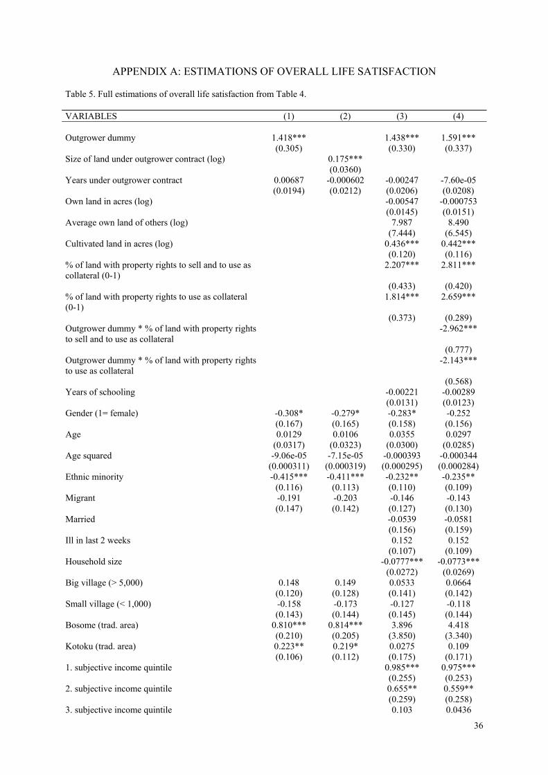
36
APPENDIX A: ESTIMATIONS OF OVERALL LIFE SATISFACTION
Table 5. Full estimations of overall life satisfaction from Table 4.
VARIABLES (1) (2) (3) (4) Outgrower dummy 1.418*** 1.438*** 1.591*** (0.305) (0.330) (0.337) Size of land under outgrower contract (log) 0.175*** (0.0360) Years under outgrower contract 0.00687 -0.000602 -0.00247 -7.60e-05 (0.0194) (0.0212) (0.0206) (0.0208) Own land in acres (log) -0.00547 -0.000753 (0.0145) (0.0151) Average own land of others (log) 7.987 8.490 (7.444) (6.545) Cultivated land in acres (log) 0.436*** 0.442*** (0.120) (0.116) % of land with property rights to sell and to use as collateral (0-1)
2.207*** 2.811***
(0.433) (0.420) % of land with property rights to use as collateral (0-1)
1.814*** 2.659***
(0.373) (0.289) Outgrower dummy * % of land with property rights to sell and to use as collateral
-2.962***
(0.777) Outgrower dummy * % of land with property rights to use as collateral
-2.143***
(0.568) Years of schooling -0.00221 -0.00289 (0.0131) (0.0123) Gender (1= female) -0.308* -0.279* -0.283* -0.252 (0.167) (0.165) (0.158) (0.156) Age 0.0129 0.0106 0.0355 0.0297 (0.0317) (0.0323) (0.0300) (0.0285) Age squared -9.06e-05 -7.15e-05 -0.000393 -0.000344 (0.000311) (0.000319) (0.000295) (0.000284) Ethnic minority -0.415*** -0.411*** -0.232** -0.235** (0.116) (0.113) (0.110) (0.109) Migrant -0.191 -0.203 -0.146 -0.143 (0.147) (0.142) (0.127) (0.130) Married -0.0539 -0.0581 (0.156) (0.159) Ill in last 2 weeks 0.152 0.152 (0.107) (0.109) Household size -0.0777*** -0.0773*** (0.0272) (0.0269) Big village (> 5,000) 0.148 0.149 0.0533 0.0664 (0.120) (0.128) (0.141) (0.142) Small village (< 1,000) -0.158 -0.173 -0.127 -0.118 (0.143) (0.144) (0.145) (0.144) Bosome (trad. area) 0.810*** 0.814*** 3.896 4.418 (0.210) (0.205) (3.850) (3.340) Kotoku (trad. area) 0.223** 0.219* 0.0275 0.109 (0.106) (0.112) (0.175) (0.171) 1. subjective income quintile 0.985*** 0.975*** (0.255) (0.253) 2. subjective income quintile 0.655** 0.559** (0.259) (0.258) 3. subjective income quintile 0.103 0.0436

37
(0.192) (0.194) 4. subjective income quintile 0.104 0.113 (0.173) (0.177) Average subjective income of others 5.194 6.325 (6.253) (5.473) Aggregated assets (log) 0.139* 0.129* (0.0717) (0.0684) Constant 5.071*** 6.337*** -28.05 -32.53 (0.759) (0.814) (33.24) (29.08) Observations 824 824 824 824 R-squared 0.209 0.215 0.357 0.376 Note: The estimator is OLS. Clustered standard errors at village level in parentheses; significance levels at:*** p<0.01, ** p<0.05, * p<0.1; reference categories: main ethnicity: Akan, traditional area: Abuakwa, village: small, subjective income: poorest quintile.
APPENDIX B. ROBUSTNESS CHECKS
Table 6. Further estimations of overall life satisfaction
VARIABLES (1) (2) (3) (4) Ordered OLS OLS OLS logit
full sample excluding extreme
landowners landowners
only land less
only Outgrower dummy 1.857*** 1.565*** 1.201*** 2.025*** (0.452) (0.346) (0.425) (0.508) Years under outgrower contract 0.00118 0.00315 0.0255 -0.0243 (0.0267) (0.0213) (0.0231) (0.0283) Own land in acres (log) 0.00113 -0.00191 -0.103 (0.0162) (0.0154) (0.0709) Average own land of others (log) 8.769 9.057 7.033 (9.678) (7.412) (7.150) Cultivated land in acres (log) 0.479*** 0.445*** 0.507*** 0.439** (0.145) (0.114) (0.118) (0.191) % of land with property rights to sell and to use as collateral(0-1)
3.193*** 2.850*** 2.877***
(0.494) (0.413) (0.445) % of land with property rights to use as collateral (0-1)
2.922*** 2.689*** 2.743***
(0.399) (0.282) (0.318) Outgrower dummy * % of land with property rights to sell and collateral
-3.820*** -2.924*** -3.337***
(0.812) (0.753) (0.745) Outgrower dummy * % of land with property rights to use as collateral
-2.155*** -2.083*** -2.174***
(0.827) (0.623) (0.624) Years of schooling -0.00257 -0.00187 -0.00689 0.00533 (0.0163) (0.0125) (0.0161) (0.0172) Gender (1= female) -0.277 -0.289* -0.0361 -0.689** (0.196) (0.162) (0.212) (0.256) Age 0.0341 0.0357 0.0304 0.0588 (0.0387) (0.0320) (0.0295) (0.0562) Age squared -0.000395 -0.000412 -0.000343 -0.000661 (0.000389) (0.000321) (0.000293) (0.000575) Ethnic minority -0.240* -0.227** -0.204 -0.171 (0.132) (0.112) (0.169) (0.192) Migrant -0.116 -0.173 -0.0136 -0.377** (0.161) (0.134) (0.181) (0.186)

38
Married -0.0430 -0.0576 -0.0648 -0.00421 (0.184) (0.164) (0.217) (0.266) Ill in last 2 weeks 0.103 0.140 0.252* -0.0104 (0.134) (0.112) (0.143) (0.167) Household size -0.0831** -0.0846*** -0.0844** -0.0747* (0.0367) (0.0260) (0.0342) (0.0386) Big village (> 5,000) 0.0754 0.0440 0.0653 0.0680 (0.184) (0.144) (0.173) (0.238) Small village (< 1,000) -0.0903 -0.133 -0.0633 -0.301 (0.187) (0.146) (0.210) (0.194) Bosome (trad. area) 4.743 4.631 4.329 -0.0541 (4.934) (3.708) (3.332) (1.378) Kotoku (trad. area) 0.209 0.0820 0.219 -0.0132 (0.213) (0.183) (0.225) (0.481) 1. subjective income quintile 1.297*** 0.904*** 1.366*** 0.176 (0.330) (0.256) (0.234) (0.449) 2. subjective income quintile 0.753** 0.536** 0.671** 0.514 (0.332) (0.263) (0.270) (0.347) 3. subjective income quintile 0.0426 0.0128 0.171 -0.0418 (0.238) (0.190) (0.267) (0.237) 4. subjective income quintile 0.242 0.0960 0.238 0.0664 (0.229) (0.179) (0.210) (0.314) Average subjective income of others 7.171 6.600 6.530 -2.082 (7.905) (6.057) (5.187) (3.477) Aggregated assets (log) 0.160* 0.118* 0.136* 0.146 (0.0835) (0.0693) (0.0789) (0.0986) Constant 37.08 -34.41 -31.01 9.351 (42.42) (32.50) (28.94) (11.21) Observations 824 809 483 341 R-squared 0.374 0.457 0.300 Note: Clustered standard errors at village level in parentheses; significance levels at: *** p<0.01, ** p<0.05, * p<0.1; reference categories: main ethnicity: Akan, traditional area: Abuakwa, village: small, subjective income: poorest quintile. In model (2) extreme landowners with own land > 30 acres are excluded. In model (3) landless farmers are excluded, whereas model (4) excludes landowners.

1
Appendix D: Experimental Protocol
GENERAL INTRODUCTION
Thank you all for coming today. My name is Sovanno, this is Phara, this is Chettra and
this is Simone. Simone is a researcher of the University of Marburg in Germany. In this
workshop today, we want to play a game where you can earn a considerable amount of money
that you are permitted to keep and take home. In this game you will have to make decisions
that will influence your personal outcome. The whole procedure will last for two to three
hours. After the game we are also going to offer you free food to thank you for your effort and
time.
You should understand that the money you can earn in the game is not Simone’s own
money. It is money given to her by her university to do a research study, which will
eventually be part of a book. The game is research and not part of the LASED project.
Before we start to explain the game, we want to announce some general rules that you
should know:
• If at any time you find that this is something that you do not wish to participate in for
any reason, you are of course free to leave whether we have started the game or not.
But if you feel uncomfortable already now, or you know that you will not be able to
stay for the two to three hours, then you should not participate.
• During the game talking is strictly prohibited. You cannot ask questions or talk about
the rules of the game while we are in the process of playing. If you have any
questions, please raise your hand and wait until someone comes to answer your
question in private. A violation of this rule will lead to the exclusion from the game
and the payments.
• You are asked to fill in a questionnaire before the game and after the game. Before
you get handed out your money at the end of the game, all parts of the questionnaire
should be completed. It is very important for our research, that you answer all
questions seriously.
After knowing these rules, is there anybody who does not like to participate anymore?

2
During the game we are going to use a die. This is what the die looks like [show die].
A die has six sides each of it has the same size and shape. Therefore, the probability for each
side to be drawn is 1/6. On each side of the die you can see a number. The numbers range
from 1 to 6. If you throw a die the important number is the one which you see at the top of the
die. This means: the number thrown is the number which you can see by looking at the die
from above. I will throw the die three times to show you how it works [throw die to show
example and explain the number on top]. During this game your payouts will be determined
by throwing the die.
The game consists of several games and lasts between two to three hours. You can get
money in each game depending on your decisions; however just one game is finally paid out.
After the game we randomly determine which of these games will be paid out to you by
throwing the die. In all games you can earn money and you cannot lose any money. While
you are answering the questionnaire at the end of the game, one by one will come to Simone
and Phara, who will hand out the earnings to you and you sign the receipt. You will be paid
the earnings from one of the games that you have played during the game.
After we have read aloud the instructions for the first game of the game, all of you will
receive a player number. You keep the same player number for all three games of the game. It
is very important that you don’t show your player number to anybody else. In order to get
your earnings, you have to show Simone and Phara your player number, so that she can
determine your earnings.
All the games have something in common: The decision you have to make is a bit like
the decision that you as a farmer have to make this year when it is time to plant your rice.
There are traditional and new seed varieties on the market. The traditional varieties are easy to
predict and give average yields for this kind of soil. The new rice varieties are less
predictable. Maybe they don’t fit to the soil and hence only give low yields; on the other hand
they might bring higher yields than the traditional varieties if the soil fits. You as a farmer
have to decide whether to take the risk and plant a new variety that will give you a good
income, but only if it fits to the soil, or to play it safe and take a traditional variety which will
give you a moderate income regardless of the soil condition. Deciding which variety to plant
is like playing a game of chance.
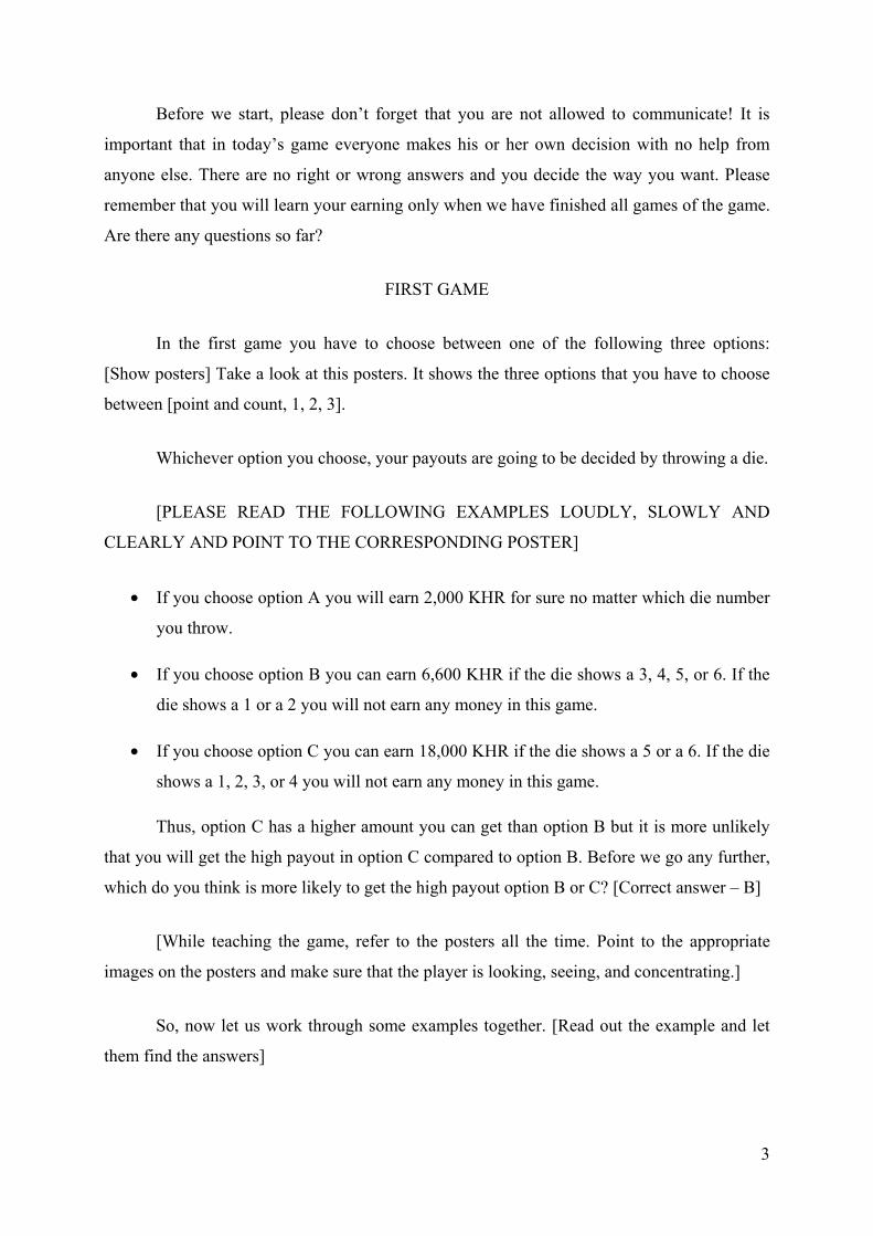
3
Before we start, please don’t forget that you are not allowed to communicate! It is
important that in today’s game everyone makes his or her own decision with no help from
anyone else. There are no right or wrong answers and you decide the way you want. Please
remember that you will learn your earning only when we have finished all games of the game.
Are there any questions so far?
FIRST GAME
In the first game you have to choose between one of the following three options:
[Show posters] Take a look at this posters. It shows the three options that you have to choose
between [point and count, 1, 2, 3].
Whichever option you choose, your payouts are going to be decided by throwing a die.
[PLEASE READ THE FOLLOWING EXAMPLES LOUDLY, SLOWLY AND
CLEARLY AND POINT TO THE CORRESPONDING POSTER]
• If you choose option A you will earn 2,000 KHR for sure no matter which die number
you throw.
• If you choose option B you can earn 6,600 KHR if the die shows a 3, 4, 5, or 6. If the
die shows a 1 or a 2 you will not earn any money in this game.
• If you choose option C you can earn 18,000 KHR if the die shows a 5 or a 6. If the die
shows a 1, 2, 3, or 4 you will not earn any money in this game.
Thus, option C has a higher amount you can get than option B but it is more unlikely
that you will get the high payout in option C compared to option B. Before we go any further,
which do you think is more likely to get the high payout option B or C? [Correct answer – B]
[While teaching the game, refer to the posters all the time. Point to the appropriate
images on the posters and make sure that the player is looking, seeing, and concentrating.]
So, now let us work through some examples together. [Read out the example and let
them find the answers]

4
• Now, imagine that you choose option A. Then we throw a die. You throw a 1,2,3,4,5,
or 6 so you get how much? [Correct answer is 2,000 KHR]
• Now, imagine that you choose option C. Then we throw a die. You throw a 1,2,3, or 4
so you get how much? [Correct answer is 0 KHR] And what if you throw a 5 or a 6,
how much would you get then? [Correct answer is 18,000 KHR.]
• Now, imagine that you choose option B. Then we throw a die. You throw a 1 or a 2 so
you get how much? [Correct answer is 0 KHR] And what if you throw a 3,4,5, or 6,
how much would you get then? [Correct answer is 6,600 KHR.]
Phara will accompany you to the place where you will play the game with Simone. At
first she will test whether you have understood the game. Then you have to make your actual
decision between option A, B, or C.
After you have made the decision on the option you would like to choose you will
throw the die inside this box [show box and die] in a way that Simone and you can see the
outcome. If there are any difficulties with the die, e.g. not clear which side is on top, the die is
thrown again. Remember, this is a normal die, i.e. it is numbered from 1 to 6. The probability
for each number to be drawn is with 1/6 the same for each number. The number thrown is the
number which you can see by looking at the die from above. The number of the die is
compared to the chosen option. If the number yields a profit your profit is noted on your
earnings account, otherwise Simone will note zero as gain.
After your game you have to wait in the waiting area until everybody has played the
game and someone comes and brings you back to the room here. Please don’t discuss your
choices during this time, so please don’t talk. If you violate this rule we have to exclude you
from the game and the payments.
[AFTER EVERYONE MADE THEIR DECISION THE INSTRUCTIONS FOR THE 2ND
GAME ARE PRESENTED]
Let’s turn to the second game:
The second game is similar to the first one. Again you have to choose among the same
three options. [Show posters] Take a look at these posters. They show the three options that
you have to choose between [point and count, 1, 2, 3].

5
Whichever option you choose, your payouts are going to be decided by throwing a die.
In this game there is one additional rule: each participant of our game is a member of a
three-person-group which is formed randomly. You are randomly matched with two other
participants in this room– these will be your partners for this game. You will not learn the
identity of the participants you are matched with, and vice versa your partners will never learn
about your identity. Only Simone will know who your partners are, but she will not tell
anybody, neither now nor after the end of the game.
First you have to choose one of the three options on the posters. [Refer to posters
again]. However, after throwing your die and knowing your payoff and if you got the high
payout, we ask you to state how much you are willing to hand over voluntarily from your
payouts to those players who receive 0 payout in your three person group. You have to take
this decision for the case of one person who got 0 payout in your group and for the case of
two people who got 0 payout in your group always depending on the option the other players
in your group choose. The other members in your group have to take the same decisions. No
more than your earnings of this game can be transferred in total. If you like you can also
choose to transfer nothing to people who got 0 payout.
Please have a look at these posters [show posters on solidarity]. Since you have to take
this decision without knowing how many people in your group got 0 payout and which option
they choose there are the following five transfer choices you have to make.
• Suppose there is one person who got 0 payout in your three person group and he
chooses option B. How much are you willing to transfer? [Point to the corresponding
poster.]
• Suppose there is one person who got 0 payout in your three person group and he
chooses option C. How much are you willing to transfer? [Point to the corresponding
poster.]
• Suppose there are two people who got 0 payout in your three person group. Both of
them choose option B. How much are you willing to transfer to each of them? [Point
to the corresponding poster.]

6
• Suppose there are two people who got 0 payout in your three person group. One of
them chooses option B and the other one option C. How much are you willing to
transfer to the player who chooses option B and how much are you willing to transfer
to the player who chooses option C? [Point to the corresponding poster.]
• Suppose there are two people who got 0 payout in your three person group. Both of
them choose option C. How much are you willing to transfer to each of them? [Point
to the corresponding poster.]
If you get the high payout, you receive your earnings from the game possibly minus
your voluntary transfer to the people in your group who got 0 payout. If you get 0 payout, you
receive the transfers of the members in your group who got more than 0 payout.
1st Example [Point to the corresponding poster.]:
• Suppose the first player chooses option C and throws a 2.Thus, he gets 0 payout and
has no money in this game.
• Suppose the second player in the group chooses option A and throws a 5. No matter
which number he throws he gets 2,000 KHR in this game.
• Suppose the third player in the group chooses option B and throws a 4.Thus, he gets
6,600 KHR in this game.
Now imagine the second player decides to give 100 KHR in the case that there is one
player with 0 payout who chooses option C in the three person group. The third player
decided to give 500 KHR in the case that there is one player with 0 payout who chooses
option C in the three person group. Then Player one earns 600 KHR in this game
(0+100+500). Player 2 earns 1,900 KHR in this game (2,000-100) and Player 3 earns 6,100
KHR (6,600-500).
2nd Example [Point to the corresponding poster.]:
• Suppose the first player chooses option A and throws a 6. No matter which number he
throws he gets 2,000 KHR in this game.
• Suppose the second player in the group chooses option B and throws a 2.Thus, he has
0 payout and has no money in this game.

7
• Suppose the third player in the group chooses option C and throws a 1.Thus, he has 0
payout and has no money in this game.
Now imagine the first player decides in the case that two players receive 0 payout, to
give 200 KHR to a player who has chosen option B and to give 500 KHR to a player who has
chosen option C. Then Player one earns 1,300 KHR (2,000-200-500) in this game. Player 2
earns 200 KHR in this game (0+200) and Player 3 earns 500 KHR (0+500).
3rd Example [Point to the corresponding poster.]:
• Suppose the first player chooses option B and throws a 4. Thus, he gets 6,600 KHR in
this game.
• Suppose the second player in the group chooses option C and throws a 3.Thus, he has
0 payout and has no money in this game.
• Suppose the third player in the group chooses option C and throws a 1.Thus, he has 0
payout and has no money in this game.
Now imagine the first player decides in the case that two players receive 0 payout, to
give 600 KHR to each player who has chosen option C. Then Player one will have earned
5,400 KHR (6,600-600-600) in this game. Player 2 earns 600 KHR in this game (0+600) and
Player 3 earns also 600 KHR (0+600).
4th Example [Point to the corresponding poster.]:
• Suppose the first player chooses option C and throws a 6. Thus, he gets 18,000 KHR
in this game.
• Suppose the second player in the group chooses option A and throws a 2. No matter
which number he throws he gets 2,000 KHR in this game.
• Suppose the third player in the group chooses option B and throws a 5.Thus, he gets
6,600 KHR in this game.
In this game all three players receive payouts bigger than 0. Thus, no transfers are paid
and each player earns according to his payouts.
5th Example [Point to the corresponding poster.]:

8
• Suppose the first player chooses option C and throws a 3. Thus, he has 0 payout and
has no money in this game.
• Suppose the second player in the group chooses option A and throws a 5. No matter
which number he throws he gets 2,000 KHR in this game.
• Suppose the third player in the group chooses option A and throws a 3. No matter
which number he throws he gets 2,000 KHR in this game.
Now imagine the second player decides to give nothing in the case that one player
who chooses option C has 0 payout and the third player decides to give 300 KHR in case one
player who chooses option C has 0 payout. Then Player one will have earned 300 KHR
(0+300) in this game. Player 2 will earn 2,000 KHR in this game and Player 3 will earn 1,700
KHR in this game (2,000-300).
Now after these examples an assistant will accompany you to the place where we play
the game: Then Simone and Phara will check whether you understand the principle of the
transfers. Afterwards you will choose which option you want to take. You roll the die and
Simone and Phara tell you your payout. In case of a payout bigger than 0 you make the
decisions on your transfers. You decide on how much you transfer to one player with 0 payout
in your group if he chooses option B or if he chooses option C. For the case of two people
who get 0 payout you decide how much you would transfer per player to two players who
choose option B, to one player who chooses option B and one player who chooses option C,
and to two players who choose option C. In case you got 0 payout in this game of the game,
Simone and Phara will ask you how much transfer you expect from a group member who gets
more than 0 payout if he chooses option A, B or C in case of one and in case of two players
with 0 payout. After having played the game we ask you to leave the decision room and stay
some time outside. An assistant will accompany you to the waiting area. As soon as
everybody has made a decision and played the game an assistant will bring you back. Please
don’t discuss your decisions during the waiting time. Otherwise we have to exclude you from
the game and the payment.
[AFTER EVERYONE MADE THEIR DECISION THE INSTRUCTIONS FOR THE 3RD
GAME ARE PRESENTED]
I welcome you to the third game of the game.

9
In this game each participant of our game is again a member of a three-person-group
which is newly formed by random. As before, you will not learn the identity of the
participants you are matched with, and vice versa your partners will never learn about your
identity. Only Simone will know who your partners are, but she will not tell anybody, neither
now nor after the end of the game.
This game is similar to the one before as you can also give transfers to the other two
group members in case they get 0 payout in this game. However, this game is different from
the last one as you do not use a die to determine payouts but you rather have to solve a
specific task. This task consists of throwing a ball into this bucket [show bucket]. To receive a
certain payoff you have to hit the bucket for a specified number of times. We have played the
game before and found out that in average people hit the bucket 5 times. Before throwing the
ball you have to choose one of the following three options:
[Show posters] Take a look at this poster. It shows the three options that you have to
choose between [point and count, 1, 2, 3].
Whichever option you choose, your payouts are determined by the times you hit the
bucket.
[PLEASE READ THE FOLLOWING EXAMPLES LOUDLY, SLOWLY AND
CLEARLY AND POINT TO THE POSTER]
• If you choose option A you will earn 2,000 KHR for sure no matter how often you hit
the bucket.
• If you choose option B you can earn 6,600 KHR if you hit the bucket for at least 4
times. 2/3 of the people from the pre-test hit the bucket at least 4 times. If you hit the
bucket for less than 4 times you get 0 payout.
• If you choose option C you can earn 18,000 KHR if you hit the bucket for at least 7
times. 1/3 of the people from the pre-test hit the bucket at least 7 times. If you hit the
bucket for less than 7 times you get 0 payout.
Thus, for option A you do not need to hit the bucket to get the payout. But if you
choose option B or C getting the high payout depends on the times you hit the bucket. For

10
option C you have to hit it at least 7 times whereas for option B only 4 times. Thus option B is
easier to accomplish but for option C the payout is higher.
Please make sure that you understand that if you choose option C and you hit the
bucket less than 7 times but more than 4 times you do not get any payout.
[While teaching the game, refer to the poster all the time. Point to the appropriate
images on the poster and make sure that the player is looking, seeing, and concentrating.]
So, now let us work through some examples together.
• First, imagine that a player chooses option B. Then he throws the ball 10 times. He
hits the bucket for 3 times. How much payout does he get? [Correct answer is 0 KHR]
And what if he hits the bucket 5 times, how much would he get then? [Correct answer
is 6,600 KHR.]
• Now, imagine that you choose option A. Then you throw the ball and hit the bucket 2
times, so you win how much? [Correct answer is 2,000 KHR] And what if you hit the
bucket 9 times, how much would you win then? [Correct answer is 2,000 KHR.]
• Now, imagine that a player chooses option C. Then he throws the ball 10 times. He
hits the bucket 6 times. How much payout does he get? [Correct answer is 0 KHR]
And what if he hits the bucket 7 times how much would he get then? [Correct answer
is 18,000 KHR.]
• Now, imagine that a player chooses option C. Then he throws the ball 10 times. He
hits the bucket for 9 times. How much payout does he get? [Correct answer is 18,000
KHR]
First you have to choose one of the three options on the poster. [Refer to poster again].
However, after playing the game and knowing your payout if you got the high payout we ask
you to make the same transfer decision as in the previous game: how much you are willing to
hand over voluntarily from your payout to those players who receive 0 payout in your three
person group?
We will now ask you one by one to go to Simone and Phara to make your option
decision. You play the game and Simone and Phara tell you your payout. Then you make

11
decisions on your transfers in case of a payout bigger than 0. You decide on how much you
transfer to one person with 0 payout in your group if he plays option B or if he plays option C.
For the case of two people who get 0 payout you decide how much you would transfer per
player to two players who choose option B, to one player who chooses option B and one
player who chooses option C, and to two players who choose option C. After having played
the game we ask you to leave this decision room and stay some time outside. An assistant will
accompany you to the waiting area. Here Chettra and I will ask you the questions from our
questionnaire. Please don’t talk with the other participants about your choices. In case of
violation of this rule we have to exclude you from the game and from the payments.
AFTER EVERYBODY MADE THE DECISION IN GAME 3
As mentioned before, we will now throw a die to determine which of the three games
will be paid out to all of you. We will only throw one die and the result will be binding for
everyone in the group. Die numbers 1 and 2 mean that you are paid out your first game, 3 and
4 will give you your earnings of the 2nd game, numbers 5 and 6 give you the earnings of the
3rd (and last) game.
For example, if you earned 3,000 KHR in game 1, 4,000 KHR in game 2 and 2,000
KHR in game 3. We will throw the die to determine whether we will pay everybody
according to their payouts in game 1, game 2 or game 3. If the die shows a 5 then everybody
will be paid the third game earning. For our example this would mean that the person gets
2,000 KHR from game 3.
[Throw die/or let it throw by someone unanimous] Ok, the die number is …. We will
pay you the earnings from game …. Please give me some time to calculate your earnings and
prepare the money. In the meantime we will carry on with asking the questionnaire.
Thanks for your participation!
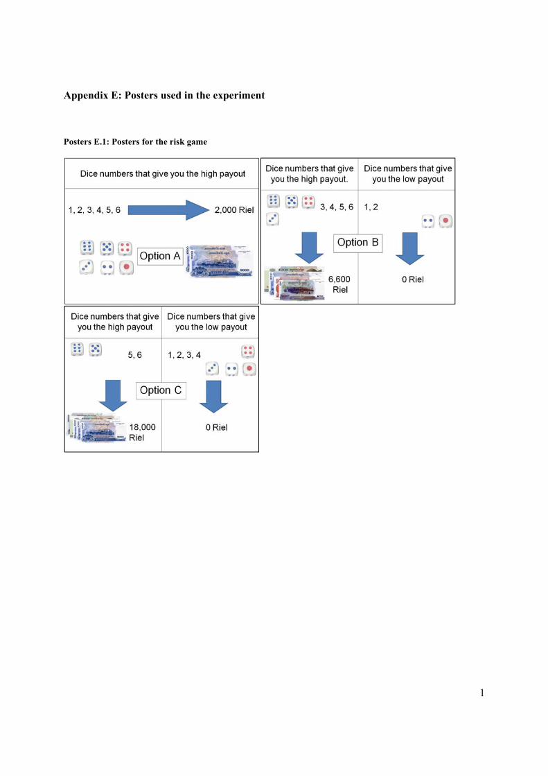
1
Appendix E: Posters used in the experiment
Posters E.1: Posters for the risk game

2
Posters E.2: Posters for the solidarity game

3
Posters E.3: Examples for the solidarity game

4
Posters E.4: Posters for the skilled task