land cover change and hydrological regimes in the …
TRANSCRIPT

LAND COVER CHANGE AND HYDROLOGICAL
REGIMES IN THE SHIRE RIVER CATCHMENT,
MALAWI
Lobina Getrude Chozenga Palamuleni
Student Number 920418079
A thesis submitted in fulfilment of the requirements for the degree of Doctor of
Philosophy in the Department of Geography, Environmental Management and
Energy Studies, University of Johannesburg.
Supervisor: Professor Harold John Annegarn
Johannesburg, 20 March 2009

i
Declaration
I declare that the work contained in this thesis is my own original writing. Sources
referred to in the creation of this work have been appropriately acknowledged by
explicit references or footnotes. Other assistance received has been acknowledged. I
have not knowingly copied or used the words or ideas of others without such
acknowledgement.
Signed ___________________ Date __________________
Sections of this work have been presented at conferences and have been submitted for
Journal publication:
Palamuleni, L. G., T. Landmann and H. J. Annegarn, (2006), Land cover
mapping for the Shire River catchment in Malawi using Landsat
satellite data, Palamuleni, L. G., T. Landmann and H. J. Annegarn,
(2008), Awarded the Best Paper at the 6th African Association of
Remote Sensing of the Environment (AARSE) Conference, 30 October
-2 November 2006, Cairo, Egypt.
Palamuleni, L. G., T. Landmann and H. J. Annegarn, (2007), Mapping rural
savanna woodlands, a comparison of maximum likelihood and fuzzy
classifiers, International Geoscience and Remote Sensing Symposium
(IGARSS’07), 23-27 July 2007, Barcelona, Spain
Palamuleni, L. G., T. Landmann and H. J. Annegarn, (2008), An assessment
of land cover change using multi-temporal Landsat imagery for the
Shire River catchment, Malawi, 7th African Association of Remote
Sensing of the Environment (AARSE) Conference, 27 - 30 October
2008, Accra, Ghana.
Palamuleni, L. G., T. Landmann and H. J. Annegarn, (2008), Processing
changes in land cover using Landsat imagery for the Shire River
catchment, Malawi. Paper submitted to Journal of Applied Earth
Observation and Geoinformation.
Palamuleni, L. G., H. J. Annegarn, T. Landmann amd P. M. Ndomba, (2008),
Application of the AVSWATX Tool for the Shire River Sub-Catchment in
Malawi. Paper submitted to Hydrological Sciences Journal.

ii
Dedication
To my husband, Dr Martin E. Palamuleni, for showing me the path to greatness
and
to my sister, Rhoda, and my lovely daughters Tadala and Tamanda
for encouraging me against all odds

iii
Abstract
Land cover changes associated with growing human populations and expected
changes in climatic conditions are likely to accelerate alterations in hydrological
phenomena and processes on various scales. Subsequently, these changes could
significantly influence the quantity and quality of water resources for both nature and
human society. Documenting the distribution of land cover types within the Shire
River catchment is the foundation for applications in this study of the hydrology of the
Shire catchment.
The aim of this study is to investigate the relationships between the measured land
cover changes and hydrological regimes in the Shire River Catchment in Malawi.
Maps depicting land cover dynamics for 1989 and 2002 were derived from multi-
spectral and multi-temporal Landsat 5 (1989) and Landsat 7 ETM+ (2002) satellite
remote sensing data for this catchment. Other spectral-independent data sets included
the 90-m resolution Shuttle Radar Topographic Mission (SRTM) digital elevation
model (DEM), Geographical Information System (GIS) layers of soils, geology and
archived land cover. Core image-derived data sets such as individual Landsat bands,
Normalized Difference Vegetation Index (NDVI), Principal Components Analysis and
Tasseled Cap transformations were computed. From generated composite images,
land cover classes were identified using a maximum likelihood algorithm. Eight land
cover classes were mapped.
A hierarchical multispectral shape classifier with an object conditional approach
determined by the Food and Agriculture Organisation (FAO) Land Cover
Classification System (LCCS) legend structure was used to map land cover variables.
LCCS was used as a basis for classification to achieve legend harmonization within
Africa and on a global scale. Flexibility of the hierarchical system allowed
incorporation of digital elevation objects, soil and underlying geological features as
well as other available geographical data sets. This approach improved classification
accuracy and can be adopted to discriminate land cover features at several scales,
which are internally relatively homogeneous. In addition to compatibility with the
FAO/LCCS classification system, the derived land cover maps have provided recent
iv
and improved classification accuracy, and added thematic detail compared to the
existing 1992 land cover maps.
Fieldwork was conducted to validate the land cover classes identified during
classification. Accuracy assessment was based on the correlation between ground
reference samples collected during field exercise and the satellite image classification.
The overall mapping accuracy was 87%, with individual classes being mapped at
accuracies of above 77% for both user and producer accuracy. The combination of
Landsat images, vector data and detailed ground truthing information was used
successfully to classify land cover of the Shire River catchment for years 1989 and
2002.
Quantitative changes in the areas of various land cover categories and the direction of
change were determined. Land cover change detection was carried out by Multi-date
visual compositing, followed by Post-classification analysis. For the first step,
degradation of vegetation was chosen as the main indicator of change, while post
classification statistical analysis was employed to determine the specific nature of
changes in each land cover type. Multi-date visual composites were found to detect
areas of change and of no change better than post-classification. Using the post-
classification procedure, areal statistics and direction of change in each land cover
class were derived using a combination of both methods. This activity highlights areas
where there are major changes of land cover (i.e. "hot spots"), both in temporal and
spatial aspects. The study revealed significant changes in magnitude and direction that
have occurred in the catchment between 1989 and 2002, mainly in areas of human
habitation. Trends in land cover change in the upper Shire River catchment depict
land cover transition from woodlands to mostly cultivated/grazing and built-up areas.
Twelve per cent of the total land surface of the study area had been converted to
cultivation/grazing over a 13-year interval.
Positive changes (referring to reforestation of degraded areas) in woody closed areas
especially within the former refugee areas close to the Mozambican border, provides
some evidence of the ecological sustainability of the resource. However, the reversal
of the decreasing trend in woody open and savanna shrubs has raised some questions
regarding the possible continuation of the observed trends in future. As subsistence
farming continues to play a dominant role in land cover conversion, degradation, from

v
evergreen Brachystegia woodlands to more open, dry vegetation, and to grassland
formations, will continue.
Considering the present scale of temporal and spatial change of the land cover in the
area, more continuous and comprehensive land cover change monitoring is required
with multi-spectral and multi-temporal satellite data merging. This study has provided
insights into the kind of landscape transformations that have taken place over 13
years, and will serve as input for the monitoring and proper utilisation of the Shire
River catchment for sustainable socio-economic development and water resources
management.
The land cover mapping derived from satellite images served as input for hydrological
modelling within the Shire River catchment. A GIS interface for SWAT, the ArcView
Soil and Water Assessment Tool eXtendable (AVSWATX) tool was used to model the
hydrology of the Shire catchment. Input variables for AVSWATX included digital
elevation data, soil and land cover grids, and weather data (daily rainfall, temperature,
relative humidity and wind speed). Available catchment streamflow data from 1977 to
1981 (5 years) were used for model calibration, while data from 1984 to 1985 were
used for model validation. The calibration was done at daily time-steps, for which
observed and modelled outputs were compared at Liwonde gauging station, the outlet
point of the catchment. Statistical evaluation of simulated catchment streamflows for
the calibration yielded Nash and Sutcliffe efficiencies (ENS) of 86% and 42% for the
monthly and daily predictions respectively. The Nash and Sutcliffe efficiency for the
validation period were considered acceptable, since the model was capable of
capturing 64% of the variance on monthly, and 42% on daily, observed records.
This validated simulation for 2002 land cover was used as a baseline for scenario
development of three scenarios: (i) continued land cover change at current trends
(business as usual); (ii) accelerated land cover degradation, associated with extensive
deforestation; and (iii) land cover restoration, reflection large-scale land restoration
and reforestation. Average annual and monthly modeled outputs from the alternative
scenarios were compared to the business as usual values to compute percent change in
annual values of surface flow, baseflow, and total channel discharge.
The condition of water resources in the Shire River catchment, Malawi, has been
affected adversely by rapid changes in land cover over the last two decades. A record

vi
of land cover changes that have taken place in the Shire River catchment has been
produced. The study has quantified the relationships that exist between land cover
changes and long-term changes in streamflow yield. A cost-effective set of techniques
has been demonstrated, combining satellite remote sensing for land cover mapping
and hydrological monitoring, which can be used in the formulation of policies for
sustainable land and water resources management in Malawi, and similar
environments elsewhere in Africa.

vii
Acknowledgements
I would like to express my genuine gratitude and appreciation to my thesis supervisor,
Professor Harold Annegarn of University of Johannesburg. His willingness to take me in
despite his busy schedule and not only coming in to scrutinize finished products but also
working through each chapter with me taught me a lot about thinking scientifically. Thanks to
Dr. Tobias Landmann from the University of Würzburg, Remote Sensing Chair, Germany,
who guided me in shaping my proposal into a workable project and for his continued support
during the PhD period. In spite of their tight schedule, they were able to provide guidance,
advice and help in this research project. I also really appreciate the confidence they showed in
me for launching into a research area that was completely new to me. I am indebted to your
understanding and kindness for helping me throughout this study, from beginning to
submission of this thesis.
I would also like to extend my gratitude to the University of Malawi, Chancellor College, for
allowing me study leave to do this PhD degree. In addition, my heartfelt gratitude goes to my
colleagues in the Department of Geography and Earth Sciences for their support.
My special thanks go to Mrs Melanie Kneen, Research Assistant at the University of
Johannesburg, for her major contribution to this research study. She was a great help
throughout, always providing good suggestions, advice, guidance and showing great patience.
I appreciate the journey she took me through TNTmips software applications and for
proofreading my drafts. I am also grateful to Dr P. M. Ndomba from the University of Dar es
Salaam, Tanzania for the very useful help concerning the use of AVSWATX.
I would like to thank Mr David Stevens, from United Nations Office for Outer Space Affairs
(UNOOSA), and US Geological Survey, for providing access to the Landsat TM and ETM+
images used for this study.
I would also like extend my sincere gratitude to Fatima Ferraz, a colleague who first
appreciated my work in remote sensing and water resources management. Through her
inspiration, I was able to participate in the European Space Agency “Tiger Africa Initiative”.
This initiative brought a lot of experience and inspiration in my experience as a beginner in
remote sensing and hydrology.

viii
Fieldwork would have been impossible without the support of Mr Jonathan Gwaligwali, GIS
Technician at the University of Malawi, Chancellor College, for gracefully enduring the
July/August heat associated with overhead sun and bushfires in Malawi.
I shared many good moments with fellow PhD students in the Department of Geography,
Environmental Management and Energy Studies who made my stay at the University of
Johannesburg a memorable period of my life. Thanks to the many colleagues I shared offices
with for the support and friendship: Dr. Patience Gwaze, Julião Cumbane, Matthew Ojelede,
Olusola Ololade, Joseph Kanyanga, Charles Ntui, Micky Josipovic, Philip Goyns and Charles
Paradzayi.
I wish to acknowledge the silent presence of my dad, Donald A. Chozenga for his love and
guidance in life. I wish he were still alive to share this memorable academic achievement. My
deepest gratitude and appreciation go to my dearest mum, Rennie Chozenga. I would like to
thank my lovely sisters Rhoda, Rose, Grace and brothers Dalitso and Justice for always caring
for me.
My deepest thanks go to my husband, Dr Martin Palamuleni, for his great comprehension,
love, and support during this study. To my daughters, Tadala and Tamanda, thank you so
much for enduring my absence.
Special thanks to the Malawian community studying in South Africa, Johannesburg who has
been a special pillar of strength. Thanks for all the encouragement and the prayers. My friends
who have been there for me, with even a number of you physically coming over to check on
me, thank you for your love.
I would also like to appreciate the help from Kate Pendlebury for the detailed editing and
proofreading on the draft thesis.
During my PhD study I received support from a number of people and organizations. I thank
Deutscher Akademischer Austausch Dienst (DAAD) through the African Network of
Scientific and Technological Institutions (ANSTI) for the PhD fellowship and the University
of Johannesburg for support during my stay at the University. Support was also given for
operating expenses and conference travel from the National Research Foundation through a
Focus Area Grant: FA2005040600018 “Sustainability Studies Using GIS and Remote
Sensing” to Prof H Annegarn. I am also grateful to the African Association of Remote
Sensing of the Environment (AARSE) and ITC, Netherlands, for a conference/workshop
fellowship to attend the 6th AARSE conference and the refresher course on Innovative
Applications of Remote Sensing and Geoinformation Sciences for female professionals in
Earth Sciences, in Cairo, Egypt.
Above all, I am grateful to the Lord God Almighty who is my source of strength and
wisdom. “I can do all things through Christ who strengthens me”.

ix
Contents
Declaration........................................................................................................... i
Dedication ........................................................................................................... ii
Abstract.............................................................................................................. iii
Acknowledgements ........................................................................................... vii
Contents ............................................................................................................. ix
List of Figures .................................................................................................... xi
Table of Abbreviations and Acronyms...............................................................xiv
1 Introduction 1
1.1 Water resources and sustainable development in Africa...............................1
1.2 Challenges within the Shire River catchment...............................................3
1.3 Aim and objectives......................................................................................6
1.4 Concepts and definitions..............................................................................9
1.5 Structure of thesis......................................................................................10
2 Land Cover Dynamics in the upper Shire River Catchment 11
2.1 Shire River catchment ...............................................................................11
2.1.1 Vegetation................................................................................................14
2.2 Overview of land cover mapping...............................................................17
2.2.1 Classification system ...............................................................................19 2.2.2 Earlier land cover mapping in Malawi.....................................................21
2.3 Methods ....................................................................................................23
2.3.1 Selection of satellite images.....................................................................24 2.3.2 Image processing .....................................................................................27 2.3.3 Image classification .................................................................................33 2.3.4 Land Cover Classification System...........................................................36
2.4 Results and discussions .............................................................................36
2.4.1 Transformation results .............................................................................37 2.4.2 Land cover maps ......................................................................................40 2.4.3 Description of land cover classes.............................................................43 2.4.4 Distribution of land cover categories .......................................................49 2.4.5 Thematic accuracy assessment.................................................................53
2.5 Conclusion ................................................................................................54

x
3 Land Cover Change assessment 1989-2002 58
3.1 Land cover change ....................................................................................58
3.1.1 Land cover change and hydrological response ........................................59
3.2 Land cover change detection .....................................................................62
3.3 Methodology .............................................................................................65
3.3.1 Input for change detection .......................................................................65 3.3.2 Approaches ..............................................................................................65
3.4 Results and discussion...............................................................................67
3.4.1 Image overlay...........................................................................................67 3.4.2 Post classification and land cover change areas.......................................70
3.5 Conclusion ................................................................................................84
4 Hydrological Modelling based on the Land Cover analysis 86
4.1 Introduction...............................................................................................86
4.1.1 Land cover and hydrological processes ...................................................86 4.1.2 Hydrological modelling approaches ........................................................87 4.1.3 Overview of the AVSWATX model ..........................................................90 4.1.4 Application of the AVSWATX model to the Shire River
catchment .................................................................................................96
4.2 Methodology .............................................................................................97
4.2.1 Data..........................................................................................................97 4.2.2 Model setup............................................................................................114 4.2.3 Modelling the Shire River catchment ....................................................118 4.2.4 Testing effects of land cover change......................................................120 4.2.5 Scenario generation................................................................................120
4.3 Results and discussion.............................................................................124
4.3.1 Hydrological characterization of Shire River catchment using
hydrological variables ............................................................................124 4.3.2 Modelling of the Shire River catchment ................................................126 4.3.3 Scenario outcomes .................................................................................142
4.4 Conclusion ..............................................................................................153
5 Conclusion and recommendations 155
5.1 Conclusion ..............................................................................................155
5.2 Recommendations ...................................................................................159
5.3 Concluding remarks ................................................................................163
References.......................................................................................................165

xi
List of Figures
Figure 1: Shire River hydrograph at Liwonde, 1948 to 2002 - water year beginning November each year ..................................................................................................5
Figure 2: Total annual rainfall from five rainfall gauging stations within the Shire
River catchment.........................................................................................................6
Figure 3: Location map of Shire River catchment, Malawi....................................................11
Figure 4: Population growth in three districts located within the study area..........................12
Figure 5: Location of the sample sites for primary data collection.........................................30
Figure 6: False colour images - 1989 and 2002 ......................................................................37
Figure 7: Principal component images - 2002 and 1989 ........................................................39
Figure 8: NDVI images - 1989 and 2002................................................................................40
Figure 9: Land cover maps - 1989 and 2002 ..........................................................................41
Figure 10: Woody closed ..........................................................................................................43
Figure 11: Woody open ............................................................................................................44
Figure 12: Savanna shrubs ........................................................................................................44
Figure 13: Grasslands ...............................................................................................................45
Figure 14: Marshy area .............................................................................................................45
Figure 15: Cultivated or grazing lands......................................................................................46
Figure 16: Built-up areas ..........................................................................................................46
Figure 17: Fresh water body .....................................................................................................47
Figure 18: Land cover extents - 1989 .......................................................................................48
Figure 19: Land cover extents - 2002 .......................................................................................49
Figure 20: Location map of forest reserves ..............................................................................50
Figure 21: Image overlay for the Shire River catchment: 1989 — 2002..................................68
Figure 22: Expansion of Mangochi Township into previously vegetated areas .......................69
Figure 23: Post classification change map of the Shire River catchment between 1989
and 2002 ..................................................................................................................71
Figure 24: Expansion of cultivated or grazing areas into predominantly savanna areas ..........74
Figure 25: Forest fragmentation around forest reserve areas....................................................75
Figure 26: Built-up areas expanding around Mangochi Township...........................................78
Figure 27: Increase in woody closed areas ...............................................................................79
Figure 28: Increase in built-up areas and tourism expansion around Liwonde National
Park..........................................................................................................................80
Figure 29: Overview of SWAT hydrological structure (adapted from Arnold et al.,
1998)........................................................................................................................91
Figure 30: Spatial distribution of soils within the Shire River catchment ..............................100
Figure 31: Rainfall variability in the Shire River catchment – first pattern (Data from
Department of Meteorology, Malawi)...................................................................103

xii
Figure 32: Rainfall variability in the Shire River catchment – second pattern (Data from the Department of Meteorology, Malawi) ....................................................104
Figure 33: Rainfall variability in the Shire River catchment – third pattern (Data from
the Department of Meteorology, Malawi).............................................................105
Figure 34: Weather stations and river gauging stations in the Shire River catchment ...........106
Figure 35: Time series streamflow for the Shire River Mangochi (inflow) and
Liwonde (outflow) for the period 1976 - 1981: data as received ..........................108
Figure 36: Streamflow data for 1977 - 1981, data as received ...............................................109
Figure 37: Smoothed daily streamflow data from 1977 - 1981 ..............................................111
Figure 38: Smoothed catchment streamflow data, 1977 - 1981..............................................112
Figure 39: Grid based discretisation and concept of flow path used in a cell.........................116
Figure 40: Sub-basins for the Shire River catchment .............................................................117
Figure 41: Time series plots of catchment streamflow and rainfall........................................125
Figure 42: Comparison of measured and simulated average annual water yield (mm)
by calibration and validation period......................................................................129
Figure 43: Comparison of monthly streamflows for calibration period, 1977 - 1981 ............129
Figure 44: Comparison of monthly catchment streamflows for validation period,
1984 - 1985............................................................................................................130
Figure 45: Comparison of daily catchment streamflows for calibration period 1977 - 1981......................................................................................................................131
Figure 46: Comparison of daily catchment streamflow for validation period: 1984 -
1985......................................................................................................................133
Figure 47: Simulated annual catchment streamflow for 1989 and 2002 land cover...............134
Figure 48: Rainfall variability between 1977 and 1981, referenced against long-term
mean (1976 – 2002)...............................................................................................135
Figure 49: Monthly mean, standard deviations and maxima of daily simulated
catchment streamflows for 1989 and 2002 land cover simulations.......................137
Figure 50: Comparison of simulated daily catchment streamflows for 1989 and 2002
land cover data.......................................................................................................138
Figure 51: Baseflow simulation results obtained from land degradation scenarios................144
Figure 52: Surface flow simulation results obtained from land degradation scenarios ..........145
Figure 53: Baseflow simulation results from land conservation scenarios.............................147
Figure 54: Surface flow simulation results from land conservation scenarios .......................148
Figure 55: Baseflow and surface flow simulation results from land conservation
scenarios ................................................................................................................148
Figure 56: Monthly mean, standard deviations and maxima of daily simulated
catchment streamflows for 2002 land cover scenario 7 and 8 simulations ...........150
Figure 57: Monthly mean, standard deviations and maxima of daily simulated
catchment streamflows for 2002 land cover, scenario 9 and 10 simulations ........151
Figure 58: Monthly mean, standard deviations and maxima of daily simulated
catchment streamflows for 2002 land cover, scenario 11 and 12 simulations ............................................................................................................152

xiii
List of Tables
Table 1: Refugees statistics by December 1992 ....................................................................13
Table 2: Description of Landsat 5 TM ..................................................................................26
Table 3: Description of Landsat ETM+.................................................................................26
Table 4: Correlation matrix for Landsat 7 ETM+ reflective bands .......................................38
Table 5: Correlation matrix for Landsat 5 reflective bands...................................................38
Table 6: Percentage of variance and correlation mapped to each principal
components in study area ........................................................................................38
Table 7: Land cover classes and their definitions..................................................................42
Table 8: Spatial distribution of land cover classes – 1989 and 2002.....................................48
Table 9: Error matrix for land cover classes..........................................................................55
Table 10: Assignment of Change Classification Codes of land cover for the Shire
River Catchment for 1989 and 2002 .......................................................................66
Table 11: Land cover changes of the Shire River catchment during 1989 to 2002.................72
Table 12: Areas changed into cultivated or grazing areas between 1989 and 2002................73
Table 13: Areas changed into grassland areas between 1989 and 2002..................................76
Table 14: Areas changed into savanna shrubs areas between 1989 and 2002.........................77
Table 15: Areas changed into built-up areas between 1989 and 2002 ....................................77
Table 16: Areas changed into woody open areas between 1989 and 2002 .............................81
Table 17: Areas changed into woody closed areas between 1989 and 2002...........................82
Table 18: Examples of large-scale hydrologic model applications .........................................88
Table 19: Data sets and sources for input into the AVSWATX model......................................97
Table 20: Spatial distribution of land cover classes and SWAT land cover class
codes for 1989 and 2002 .........................................................................................99
Table 21: Major soil types of the Shire River catchment and percent area covered .............101
Table 22: Soil parameters required by AVSWATX ................................................................101
Table 23: Weather stations and available data ......................................................................106
Table 24: Daily river flow data..............................................................................................107
Table 25: Characteristics of 2002 land cover data and deforestation scenarios ....................123
Table 26: Characteristics of simulated land cover forestation scenarios...............................124
Table 27: Relative sensitivity values of the optimised parameters........................................126
Table 28: Parameter values calibrated in SWAT using the auto-calibration tool..................127
Table 29: Average annual volumes obtained from calibration for 1977-1981......................128
Table 30: Parameters obtained from annual simulations for 1989 and 2002 land cover ......................................................................................................................134
Table 31: Parameters obtained from daily simulations for 1989 and 2002 land cover .........138
Table 32: Surface run-off simulated from 1989 and 2002 land cover...................................139
Table 33: Baseflow simulated from 1989 and 2002 land cover ............................................140
Table 34: Simulation results from bounding cases scenarios ................................................143
Table 35: Simulation results from land degradation scenarios..............................................144
Table 36: Simulation results obtained from land conservation scenarios .............................146

xiv
Table of Abbreviations and Acronyms AVHRR Advanced Very High Resolution Radiometer
AVSWATX ArcView Soil and Water Assessment Tool eXtendable
CGIAR Consultative Group on International Agricultural Research
DEM Digital Elevation Model
ENSO El Niño Southern Oscillation
FAO/LCCS Food and Agricultural Organisation/Land Cover Classification System
FAO/UNESCO Food and Agricultural Organisation/United Nations Education
Scientific and Cultural Organisation
GIS Geographical Information System
GLCN Global Land Cover Network
GLCF Global Land Cover Facility
GPS Global Positioning System
HRUs Hydrological Response Units
IDA International Development Association
IDP Integrated Development Planning
IGBP International Geosphere Biosphere Programme
IWRM Integrated Water Resource Management
Landsat TM Land satellite Thematic Mapper
Landsat ETM+ Land satellite Enhanced Thematic Mapper Plus
LH-OAT Latin Hypercube One-Factor-At-a-Time
MDGs Millennium Development Goals
MSG METEOSAT Second Generation
MODIS Moderate Resolution Imaging Spectroradiometer
NDBI Normalised Difference Built-up Index
NDVI Normalized Difference Vegetation Index
NOAA National Oceanic and Atmospheric Administration
PR Precipitation Radar
SADC Southern African Development Community
SAR Synthetic Aperture Radar
SCE-UA Shuffled Complex Evolution - University of Arizona
SEVIRI Spinning Enhanced Visible and Infrared Imager
SPOT Satellite Pour l'Observation de la Terre
SWAT Soil and Water Assessment Tool
SWRRB Simulator for Water Resources in Rural Basins
TRMM Tropical Rainfall Measuring Mission
USDA-ARS United States Department of Agriculture - Agricultural Research Service
UNEP United Nations Environmental Programme
UN/FAO United Nations, Food and Agricultural Organization
USDA-SCS United States Department of Agriculture - Soil Conservation Service
USGS United States Geological Survey
UTM Universal Transverse Mercator
WSSD World Summit of Sustainable Development

1
Chapter 1
1 INTRODUCTION
Chapter 1 presents the framework for integrated water resources management while
conceptualising the challenges of water resources in Africa in an era of growing
population and climate change. This research addresses these challenging needs within
the upper Shire River catchment in Malawi. Fundamental issues relating to land cover
change and land surface hydrological response have been summarised. Within this
context, the research hypothesis and objectives are articulated. The chapter ends with
an outline of the thesis structure.
1.1 Water resources and sustainable development in Africa
Water resources are inextricably linked with climate change, population growth and
rainfall variability, so the prospect of global climate change has serious implications for
water resources and regional development in Africa [IPCC, 2001]. Efforts to provide
adequate water resources for Africa will confront several challenges, including population
pressure; problems associated with land use, such as erosion/siltation; and possible
ecological consequences of land-use change on the hydrological cycle [Riebsame et al.,
1994]. Assessment of management issues relating to the distribution and use of water
resources requires an integrated approach. Integrated water resources management is not
only required for analyzing consequences of the adverse natural conditions such as floods
or drought but also to assess possible strategies to make the area less vulnerable to
environmental constraints and changing climate [Tolba, 1982]. In addition, the notion of
water resources management requires the matching of water availability and water use in a
river basin [Terpstra and van Mazijk, 2001]. River basins are the preferred land surface
units for water-related regional scale studies because their drainage areas represent natural
spatial integrators or accumulators of water and associated material transports and thus
allow for the investigation of cumulative effects of human activities on the environment
[Lahmer et al., 2001]. This is the system of integrated river basin management endorsed in
Agenda 21 of Rio, 1992 and echoed at the World Summit of Sustainable Development
(WSSD), Johannesburg, South Africa in 2002.
Water availability is generally a consequence of precipitation and catchment run-off. An
aspect often forgotten in this respect is the impact of new patterns of land use and land
cover on the hydrological availability of water. There are many connections between land
surface characteristics and the water cycle. Firstly, land cover can affect both the degree of

2
infiltration and run-off following precipitation events. Secondly, the degree of vegetation
cover and the albedo (degree of absorption/reflection of sun's rays) of the surface can affect
rates of evaporation, humidity levels and cloud formation [Newson, 1992]. Any change in
land use and land cover will have correlated effects in the hydrological regimes, and
possible impacts on the habitat and ecological communities [Calder, 1992; Lorup et al.,
1998]. In essence, the degree and type of land cover influences the initiation of surface
run-off, the rate of infiltration and consequently the rate of ground water recharge [Calder,
1992].
Recent studies in the Southern African Development Community [SADC, 1995] region
have revealed that climatic and land cover changes threaten to undermine the integrity of
riverine habitats, the availability and quality of water, and agricultural productivity
[Headstreams Project, 2004]. Moreover, there are several indicators of water stress and
scarcity in the SADC region, including the amount of water available per person and the
volume ratio of water withdrawn and potentially available [IPCC, 2001]. This situation has
been attributed to increasing population, which translates into increased demand for water
supply (for domestic, agricultural and industrial use), as well as to climate change. Global
warming would induce changes in precipitation and wind patterns, changes in the
frequency and intensity of storms, ecosystem stress and species loss, reduced availability
of fresh water, and a rising global mean sea level [Ominde and Juma, 1991]. Although the
impacts may not be easily predicted, changes in weather patterns may lead to the
prevalence of severe drought conditions or extreme flood events in the SADC region. The
existence of prolonged drought periods vis-à-vis water scarcity will seriously affect
agricultural production and the socio-economic activities in the region. Malawi is one of
the southern African countries likely to experience absolute water scarcity by 2025 [SADC,
1995], which is a challenge for water resources management to sustain economic
development in the country.
To balance supply and demand for water resources and to reduce negative or undesired
effects for the environment and society, changes of actual land cover have to be studied at
all spatial scales. The land surface provides a critical role in the water cycle as it is the
level at which precipitation is redistributed into evaporation, run-off or soil moisture
storage [Verburg et al., 1999]. Thus, land use and land cover studies should be viewed as
responding to the complex interactions and feedbacks linking social and biophysical

3
processes that occur on the land [Dolman and Verhagen, 2003; Maidment, 1993]. With
increasing human activities vis-à-vis water conflicts, it is important to understand the
interactions between hydrological regimes and associated land use and land cover changes
in catchments [Rockström et al., 2002]. Such an understanding can be achieved by
integrating land use planning and water resources management. Land cover and land cover
change data represents a key variable in the management and understanding of the
environment, as well as driving many environmental models such as hydrological models
within large river basins or even for particular smaller catchments. Therefore, there is a
need to develop proper planning and management approaches within the context of
Integrated Water Resource Management (IWRM). IWRM as defined by the Global Water
Partnership [Global Water Partnership, 2005] is a process that considers the co-ordination
of development and management of water, land and related resources to enhance economic
and social welfare without jeopardising the sustainability of the ecosystem. Thus,
sustainable development of water resources is a key to the maintenance of the natural
ecosystem that supports the well-being of human populations.
1.2 Challenges within the Shire River catchment
The Shire River system, the only outlet of Lake Malawi, is probably the most important
water resource for Malawi. Hydro-electric power plants of about 200 MW generation
output, based on a firm flow of 170 m³ s-1
, have been developed on Shire River providing
98% of electricity produced and used in Malawi [Malawi Government, 2001]. This
electricity is the primary source driving the economic and industrial infrastructure and
services in the country. An estimated 20-25 m³ s-1
of water is abstracted for irrigation in the
Lower Shire valley and government sponsored smallholder schemes. Blantyre City
abstracts 1 m³ s-1
of water for both domestic and industrial use. The Shire River has also
led to the development of fisheries, water-transport and tourism industries. This translates
into an increased demand for water for diverse needs and values. When its supply is
limited in quantity or quality or its distribution is uneven, water can be a source of both
cooperation and contestation among its different users [Mulwafu et al., 2003].
Over the last three decades, the Shire River catchment has undergone considerable changes
in the structure and composition of land use and land cover [Malawi Government, 1998b].
The major driving forces are related to human population increases and rainfall variability.
The national population growth rate has been increasing from 2.7% during the 1977 census

4
to 3.2% in 1998 and is likely to double in the next twenty years [National Statistical Office,
2000]. The population density in Malawi is high – the national average density was 87
people km-² and 171 people km
-² of arable land during the 1977 and 1987 censuses
respectively [National Statistical Office, 1991]. Population density in settlements within
the Shire River catchment was recorded at over 275 people km-² during the 1998 census
[National Statistical Office, 2000].
The high population growth has translated into rapidly increasing demands from land in
terms of food, shelter, energy (fuelwood) and construction materials. Some of the
woodlands are now replaced by agricultural crops, while the grass-covered dambos have
been either overgrazed or cultivated and are left bare. Swamp vegetation has been drained
and cultivated. Studies done in 1967 estimated the woodland cover to be 74% while in
1990 the cover was estimated at 61% [Green and Nanthambwe, 1992]. These observations
suggest that woodland cover has declined by 13% between 1967 and 1990 and between
1981 and 1992 Mwanza district alone experienced 1.8% average annual deforestation rate
[Hudak and Wessman, 2000]. Much of the deforestation has been linked to conversion of
communally owned miombo woodlands into agricultural land [Desanker et al., 1997;
Place and Otsuka, 2001], while high wood demands for energy has exacerbated the
situation. Although land for agricultural production is limited to only 37% of the land area
under rain-fed cultivation at traditional management level, as much as 48% of the land was
found to be under cultivation by 1989/90 growing season [Green and Nanthambwe, 1992].
Inappropriate agricultural practices including overgrazing, mono-cropping, cultivation on
steep slopes and river banks and other marginal areas have degraded land through soil
erosion, reduced water retention and the loss of soil nutrients. Aggravating this situation is
the subsequent decrease in land holding sizes, estimated at 0.5 ha per household [Malawi
Government, 1998b].
Consequently, processes of the land hydrology such as run-off, infiltration,
evapotranspiration and interception have been modified. In most cases, this has resulted in
increased run-off, accelerated soil loss with sedimentation problems leading to reduction of
baseflows and increased incidences of flood disasters during heavy storms [Malawi
Government, 1998b]. In addition, hydropower supplies are threatened by low water flows
and sedimentation, hence power disruptions occur frequently especially in dry years
[Kaluwa et al., 1997]. Aggravating the situation is an increase in demand for water, by

5
different groups with diverse needs and values. Furthermore, it is important to note that the
flow from Lake Malawi into the Shire discontinued for a period of 22 years from 1915 to
1937 [Kidd, 1983] and almost dried up in 1997 [Malawi Government, 2001]. On the one
hand, it is hypothesised that the lack of outflow was due to the vegetation growth and
piling of sediments from the small tributaries near the source, while on the other hand, low
rainfall in the catchment area during the period prior to 1937 is said to be responsible for
the lowering of the lake levels [Sheila, 1995]. However, it is unlikely that sedimentation
would have affected the 1915-1937 occurrences due to low population and associated
agricultural activities and deforestation. A significant decline in the flow of Shire River has
been observed since 1992 (Figure 1) with mean flows as low as 130 m³ s-1
in 1997
compared to 825 m³ s-1
in 1980 and 634 m³ s-1
in 1990 [Malawi Government, 2001].
0
100
200
300
400
500
600
700
800
900
1948/1949
1951/1952
1954/1955
1957/1958
1960/1961
1963/1964
1966/1967
1969/1970
1972/1973
1975/1976
1978/1979
1981/1982
1984/1985
1987/1988
1990/1991
1993/1994
1996/1997
1999/2000
Streamflow (m3 s-1)
Figure 1: Shire River hydrograph at Liwonde, 1948 to 2002 - water year beginning November each year
In addition, recent droughts in southern Africa have been associated with the drop in river
flows [SADC, 1995]. In the last three decades, Malawi has experienced variability and
unpredictability in seasonal rainfall. There have been three significant droughts (in

6
1978/79, 1981/82, and most severe was in the 1991/92 season), frequent and increasingly
long dry spells, and an erratic onset and cessation of rainfall [Malawi Government, 2001].
Further discussion on rainfall variability within the Shire River catchment is in section
4.2.1 of this thesis. Rainfall data collected from gauges within the catchment (from 1977 to
1981) is plotted in Figure 2. This is the period that has been utilised for the hydrological
modelling in this study.
1977 1978 1979 1980 1981
500
1000
1500
2000
2500
Total annual rainfall (mm)
Ntaja
Salima
Mangochi
Balaka
Chancellor college
Figure 2: Total annual rainfall from five rainfall gauging stations within the Shire River catchment
Unprecedented rainfall variability means unexpected droughts or flooding which may in
turn produce changes in land use and land cover [Meyer and Turner, 1994]. Precipitation
variability, water scarcity and changes to the water regimes through land cover change will
seriously affect agricultural production and the socio-economic activities in the country. In
addition, such variations influence the temporal phenology and chlorophyll characteristics
of the vegetation in the area, which is a challenge in remote sensing studies.
1.3 Research question, Hypothesis, Aim and Objectives
Research question
This study is intended to address the following question: What are the effects of significant
land cover changes over the past two decades on river flow characteristics that are
important for water resources, environmental functioning and hydrological processes

7
within the upper Shire River catchment? Land cover changes associated with growing
human populations and expected changes in climatic conditions are likely to accelerate
alterations in hydrological phenomena and processes on various scales. Subsequently,
these changes could significantly influence the quantity and quality of water resources for
both nature and human society. This aim will be pursued in the context of developing
integrated land use planning and water resources management in Malawi.
Hypothesis
The following general hypothesis is proposed for the Shire River catchment in Malawi:
Unsustainable changes in land cover due to human activities are significantly
altering aggregate catchment conditions, giving rise to long-term, potentially
irreversible changes in river flow characteristics.
Aim and objectives
This research hypothesis will be tested through a structured sequence of land cover change
analyses and hydrological model simulations. Accordingly, the objectives are set out as:
• To map land cover within the upper Shire River catchment for 1989 and
2002, using Landsat TM and ETM satellite imagery;
• To quantify land cover changes in the catchment between 1989 and 2002;
• To model the hydrological regimes in the upper Shire River catchment and
its sub-basins;
• To challenge the thesis hypothesis by using the hydrological model to
evaluate effects of derived quantitative land cover changes on hydrological
processes;
• To simulate likely changes to hydrological processes in response to
continued land cover changes; and
• To discuss the implications of land use management on stabilising water
regimes of the Shire River catchment.
1.4 Research Design
Land cover mapping and change detection will be based on analyses of two Landsat
images captured 13 years apart. Supplementary digital mapping data sets were obtained
from the Department of Surveys in Malawi. To map land cover dynamics, pixel based

8
classification was undertaken using Maximum Likelihood algorithm. Accuracy assessment
was carried out using producer and user accuracies for each class along with overall
accuracies [Congalton and Green, 1999]. The UN Food and Agricultural Organisation
Land Cover Classification System [Food and Agriculture Organisation, 2005] was used to
label land cover variables to achieve legend harmonisation within Africa and on a global
scale. The new classification is also internally consistent, allowing for scalability and
flexibility that can be used at different scales and different levels of detail to distinguish
land cover features.
Two approaches were utilised to detect and compare changes in the upper Shire River
catchment, namely multi-date visual composite and post-classification analysis. In the
multi-date approach, vegetation reduction was chosen as the main indicator of land cover
change. This technique is not meant to be quantitative, but rather was used to identify and
explore areas of change. Using a post-classification approach, Landsat TM and Landsat
ETM+ images were classified and labelled individually. Later, classification results were
compared on a pixel-by-pixel basis using a change detection matrix where areas of change
were extracted. Quantitative statistics were compiled to determine specific changes
between the two images i.e. magnitude and direction of change in each land cover type
[Calder, 2002].
Hydrological responses were tackled using an existing physically based hydrological
model, the Soil and Water Assessment Tool (SWAT) [Arnold et al., 1994]. This model
incorporates key features of catchment properties, including links between land cover
hydrologic responses. A Geographical Information System (GIS) interface for SWAT, the
ArcView Soil and Water Assessment Tool eXtendable (AVSWATX) tool was used to prepare
parameter input values for the Shire catchment. Input variables for AVSWATX included
digital elevation data, soil and land cover grids and weather data (daily rainfall,
temperature, relative humidity and wind speed). Five rainfall gauges were used to provide
input daily rainfall data to AVSWATX. Available catchment streamflow data from 1977 to
1981 (5 years) was used for model calibration, while data from 1984 to 1985 was used for
model validation. The calibration was done at a daily time-step where observed and
measured outputs were compared at the same outlet point on the catchment, Liwonde
gauging station. Model runs were validated using the parameterised 2002 land cover data.
This validated simulation for land cover in 2002 was used as a baseline for scenario

9
development of three scenarios: (i) continued land cover change at current trends; (ii)
accelerated land cover change associated with extensive deforestation; (iii) reduced land
cover change due to management and reforestation. Average annual outputs from three
alternative futures were then differenced from the baseline values to compute percent
change in annual values of surface flow, baseflow, and total channel discharge.
1.5 Concepts and definitions
This section describes some of the basic terminologies used in land use and land cover
research. The definitions are fundamental to fully understand and apply research results to
a broader readership. The definitions are based mainly from FAO [2005].
Land is any delineable area of the Earths’ terrestrial surface involving all attributes of the
biosphere immediately above and below this surface. It encompasses the near-surface
climate, soils and terrain, surface hydrology and human settlements patterns and physical
results of human activities. Land can be considered in two domains: (i) land in its natural
condition, (ii) land that has been modified by human beings to suit a particular use or a
range of uses.
Land use is the manner in which human beings utilise the land and its resources. Examples
of land use include agriculture, urban development, grazing, logging, and mining.
Land cover describes the physical state of the land surface. Land cover categories include
cropland, forests, wetlands, pasture, roads, and urban areas. Land cover is taken to mean a
physical description of space, of the observed (bio)-physical cover of the Earths’ surface. It
indicates what covers the land such as forest, bushes, uncultivated areas and water bodies.
Land cover classification is the process of defining land cover and land use classes based
on well-defined diagnostic criteria. A classification describes the systematic framework
with the names of the classes and the criteria used to distinguish them, and the relationship
between classes. Such information is taken from ground surveys or through remote
sensing.
Land cover change can be categorised into two types: modification and conversion. Land
cover modifications entail the changes that affect the character of the land without
changing its overall classification and can either be human induced, for example, tree
removal for logging; or have natural origins resulting from, for example, flooding, drought

10
and disease epidemics. Land cover conversion is the complete replacement of one cover
type by another such as deforestation to create cropland or pasture.
1.6 Structure of thesis
This thesis is divided into five chapters. Chapter 1 comprise of the general introduction,
which also outlines the research hypothesis and the objectives. Chapter 2 is a discussion of
land cover dynamics within the upper Shire River catchment based on a supervised
Maximum Likelihood classification of Landsat 5 TM (1989) and Landsat 7 ETM+ (2002).
The variability in spatial land cover extents for each classified land cover class between the
two periods has been examined. The results are used in chapter 3 and 4. Chapter 3 is an
examination of land cover changes within the upper Shire River catchment. The adopted
change detection methods quantitatively reveal the major changes that have occurred in the
catchment between 1989 and 2002. Chapter 4 integrates the work of the previous chapters
(2 and 3) into the preparation of parameters for the Soil Water Assessment Tool (SWAT)
hydrological model. This chapter presents the calibration, validation, and application of
SWAT model for predicting the hydrological response from land cover activities within the
catchment. Critical land cover change simulations demonstrate the capability of the model
in guiding spatially distributed land cover change and precipitation events. The final
Chapter involves the critical discussion of the main research findings and recommends
future investigations to advance the field of physically based hydrological modelling for
the management of water resources.

11
Chapter 2
2 LAND COVER DYNAMICS IN THE UPPER SHIRE RIVER
CATCHMENT
Chapter 2 provides a description of the study area, including topographical, climatic
and hydrological characteristics. An overview of land cover mapping and concepts
with regard to application of satellite data are discussed. This is followed by analyses
of land cover dynamics within the upper Shire River catchment based on a supervised
Maximum Likelihood classification of two images captured 13 years apart:
Landsat 5 TM (1989) and Landsat 7 ETM+ (2002). Differences in spatial land cover extents for each classified land cover class between the two times are examined.
2.1 Shire River catchment
Location
The Shire River catchment lies in the southern part of the Great East African Rift Valley
system and is the outlet of Lake Malawi. The river flows approximately 400 km from
Mangochi on the southern extremity of Lake Malawi, to Ziu Ziu in Mozambique at the
confluence with the Zambezi River (Figure 3). The catchment area of the basin is
18,000 km2 and is divided into upper, middle and lower sections.
Salima
Chancellor College
Balaka
Mangochi
Ntaja
Liwonde
Lake
Malawi
Lake
Malombe
Lilongwe
Zomba
Mangochi
Liwonde
Catchment boundary
Country boundary
Lilongwe
Zomba
Mangochi
Liwonde
Lilongwe
Zomba
Mangochi
Liwonde
Catchment boundary
Country boundary
Catchment boundary
Country boundary
Salima
Chancellor College
Balaka
Mangochi
Ntaja
Liwonde
Lake
Malawi
Lake
Malombe
Salima
Chancellor College
Balaka
Mangochi
Ntaja
Liwonde
Lake
Malawi
Lake
Malombe
Salima
Chancellor College
Balaka
Mangochi
Ntaja
Liwonde
Salima
Chancellor College
Balaka
Mangochi
Ntaja
Liwonde
Lake
Malawi
Lake
Malombe
Lilongwe
Zomba
Mangochi
Liwonde
Catchment boundary
Country boundary
Lilongwe
Zomba
Mangochi
Liwonde
Lilongwe
Zomba
Mangochi
Liwonde
Catchment boundary
Country boundary
Catchment boundary
Country boundary
Figure 3: Location map of Shire River catchment, Malawi

12
The upper Shire River catchment is between Mangochi and Matope, with a total channel
bed drop of about 15 m over a distance of 130 km. The focus of this study is the uppermost
reach from Mangochi to Liwonde, which is almost flat at 465 – 600 m above mean sea
level over a distance of 87 km. It forms a catchment area of 4,500 km2, located between
latitudes 14° 20' S; 15° 12' S and longitudes 34° 59' E; 35° 30' E. The river flows through
Lake Malombe, which is 1.8 m below Lake Malawi.
Population
According to administrative boundaries, the study area is located within three districts
namely: Mangochi, Machinga and Balaka. The population within these three districts has
increased from 644 177 in 1977 to 1 011 843 in 1987 and 1 218 177 in 1998 [National
Statistical Office, 2000]. The southern region of Malawi, which forms the catchment area
of the Shire River, has the highest population density ranging between 53 and 275
people km-² of arable land, varying from district to district [National Statistical Office,
2000]. Population increased by 46% from 1977 to 1998 as depicted in Figure 4. Given that
a high proportion of the population is in subsistence agriculture, an increase of population
has serious implication for the degradation of the environment.
0
100
200
300
400
500
600
700
1977
1987
1998
Population ('000)
Mangochi Machinga Balaka
Figure 4: Population growth in three districts located within the study area
13
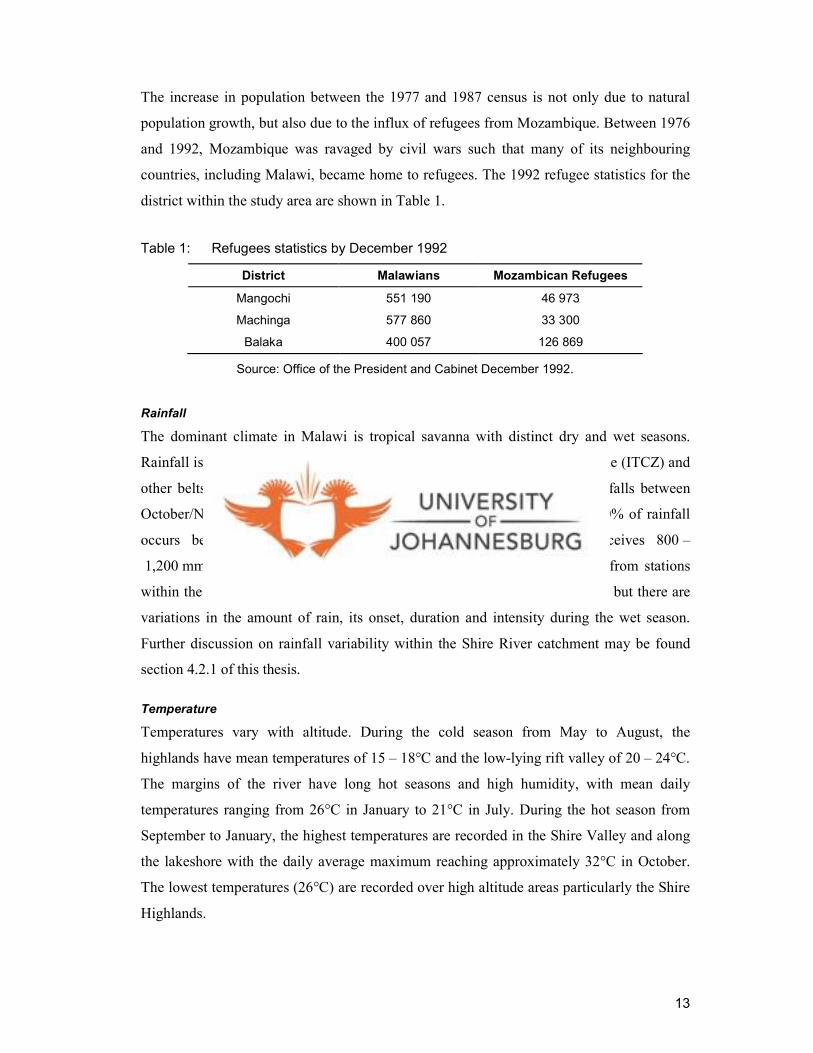
The increase in population between the 1977 and 1987 census is not only due to natural
population growth, but also due to the influx of refugees from Mozambique. Between 1976
and 1992, Mozambique was ravaged by civil wars such that many of its neighbouring
countries, including Malawi, became home to refugees. The 1992 refugee statistics for the
district within the study area are shown in Table 1.
Table 1: Refugees statistics by December 1992
District Malawians Mozambican Refugees
Mangochi 551 190 46 973
Machinga 577 860 33 300
Balaka 400 057 126 869
Source: Office of the President and Cabinet December 1992.
Rainfall
The dominant climate in Malawi is tropical savanna with distinct dry and wet seasons.
Rainfall is governed by the movement of the Inter-Tropical Convergence Zone (ITCZ) and
other belts of distribution. The onset of rain is not usually predictable but falls between
October/November and ends in April/May of the following year. Almost 90% of rainfall
occurs between December and March and most of the country receives 800 –
1,200 mm a-1
, with some exceptions [Hutcheson, 1998]. Rainfall statistics from stations
within the Shire River catchment receives an average rainfall of 996 mm a-1
, but there are
variations in the amount of rain, its onset, duration and intensity during the wet season.
Further discussion on rainfall variability within the Shire River catchment may be found
section 4.2.1 of this thesis.
Temperature
Temperatures vary with altitude. During the cold season from May to August, the
highlands have mean temperatures of 15 – 18°C and the low-lying rift valley of 20 – 24°C.
The margins of the river have long hot seasons and high humidity, with mean daily
temperatures ranging from 26°C in January to 21°C in July. During the hot season from
September to January, the highest temperatures are recorded in the Shire Valley and along
the lakeshore with the daily average maximum reaching approximately 32°C in October.
The lowest temperatures (26°C) are recorded over high altitude areas particularly the Shire
Highlands.

14
2.1.1 Vegetation
The natural vegetation in Malawi is part of the extensive dry forest Miombo woodland eco-
region, covering most of the southern and eastern parts of Africa [Abbot et al., 1995;
Desanker et al., 1997]. The Miombo woodland classification is characterised by mixed
deciduous woodlands, with dominant species from the family Caesalpinacea –
Brachystegia, Julbernardia and Isoberlinia. The vegetation types vary depending on
altitude, rainfall pattern, soil types and locations, and range from lowland rain forests,
mopane and sub-mopane woodlands, dry evergreen forests, wooded grasslands, wooded
farmlands, and swamp forests [Moyo et al., 1993].
The dominant vegetation in the study area is mopane woodland, which varies in density
from tall open woodland to dense scrub. Mopane woodlands may form pure stands
excluding other species, but are generally associated with several other prominent trees and
shrubs such as Kirkia acuminata, Dalbergia melanoxylon, Adansonia digitata, Combretum
apiculatum, C. imberbe, Acacia nigrescens, Cissus cornifolia, and Commiphora spp. The
herbaceous component of mopane communities differs according to soil conditions and
vegetation structure: dense swards are found beneath gaps in the mopane canopy on
favourable soils, while grasses are almost completely absent in shrubby mopane
communities on mopanosols [Low and Rebelo, 1996; Smith, 1998; White, 1983]. Within
the Shire highlands and the slopes along the catchment, lowland forest and Brachystegia
woodland are found.
Grasses include large tussocks of Festuca costata and Maximuella davyi interspersed with
cushions of Eragrostis volkensii and the Alloeochaete oreogena. Tall grasses are associated
with low altitude woodland, including Hyparrhenia gazensis, Hyparrhenia variabilis,
Hyparrhenia dichroa, Andropogon gayanus, Setaria palustris and Panicum maximum. In
densely settled and cultivated locations, tall reedy grasses are replaced by Urochloa
pullulans and Urochloa mosambicensis. Woodlands are characterised by Sterculia
africana, Colophospermum mopane, Acacia tortilis and Faidherbia albida according to
locality. Acacia woodland provides valuable grazing from pods to supplement grasses in
the dry season. Mature trees may stand within a dense understory, which includes
Commiphora spp., Bauhinia tomentosa, and Popowia obovata. The understory is likely to
be man-induced since lone-standing mature trees are found in open areas of cultivated
land, and in some cases trees are selectively retained by farmers to maturity (e.g.
Faidherbia albida). Base rich soils support Euphorbia ingens and Commiphora thicket,

15
whilst Hyphaene ventricosa, Hyphaene crinita and Borassus aethiopium palms occur
where the water table is high [Low and Rebelo, 1996; Smith, 1998; White, 1983].
Miombo woodlands form an integral part of the livelihood and farming systems of southern
Africa including the Shire catchment [Frost, 1996]. For most rural communities, the
woodlands are a primary source of energy in the form of fuelwood and charcoal and a
crucial source of essential subsistence goods [Dewees, 1994; Morris, 1995]. Households
rely on woodlands to supplement their food supply through the collection of wild food
plants, bushmeat, nuts, leaves and roots. Woodlands are also a source of income through
the sale of non-wood forest products such as mushrooms. Certain tree species are vital to
communities for their use as sources of traditional medicines. In commercially managed
Miombo forests, timber is a valuable product. People living in towns and cities throughout
the Miombo eco-region also depend on food, fibre, fuelwood and charcoal from miombo
woodlands [Bradley and McNamara, 1993; Dewees, 1994]. In addition, woodlands have
an ecological role in controlling soil erosion, providing shade, modifying hydrological
cycles and maintaining soil fertility [Desanker et al., 1997].
However, in recent years Miombo has been facing increasing pressure due to human
population expansion and intensive use. A large proportion of this eco-region has been
completely transformed. The various causes of deforestation include agricultural
expansion, shifting cultivation, overexploitation for fuelwood and poles, overgrazing,
excessive burning and a broad-spectrum of urban and industrial development. Although
habitat is fairly well conserved in protected areas, even national parks are affected by
people who increasingly encroach upon protected land to search for fuelwood or new
grazing and farming areas [Abbot et al., 1995]. Anthropogenic alterations together with
natural variations have transformed Miombo into open forests, thicket and grassland
formations [Frost, 1996].
Miombo woodlands present a number of cover types with similar physiognomies and their
land cover classes are usually heterogeneous at 1 km spatial resolution [Sedano et al.,
2005]. As a subtropical ecosystem, Miombo woodlands are characterised by a distinct dry
season. During this dry season, the vegetation experiences important phenological changes.
The magnitude and pace of these changes varies for every type of vegetation depending on
their capacity to reach water resources [Frost, 1996]. The characteristic phenology of every
land cover can be used in multi-temporal remote sensing approaches for land surface

16
classification. Conversely, the classification of such landscapes using remote sensing data
is likely to be affected by the reflectance patterns of different vegetation types that vary
during the dry season.
In addition, where woodlands are disappearing, landscapes are dominated by medium to
tall grasslands with forest relics and isolated stands of shrub-lands. In close association
with the woodlands, altered landscapes include village settlements (both clustered and
scattered) with grass-thatched roofing, mud walls and occasionally iron sheet roofing.
Consequently, the dormant living plants, natural leaf and grass litter, and human utilisation
of biomass products in structures exhibit intergraded classes that are internally
heterogeneous. Spectral responses recorded by remote sensing reveal similar spectral
responses that may relate to different classes. The mixture of spectral signal made up of
grass, leaf and twig litter, and bare soil constitutes a challenge for spectral image analysis
in the mapping of such landscapes. The ambiguities of land cover composition lead to land
cover classification errors.
Soils
The upper Shire River catchment is associated with the four main classes of soils: latosols,
lithosols, calcimorphic and hydromorphic soils [Malawi Government, 1998b].
Latosols and ferrosols are red-yellow soils, which include the ferruginous soils in the
upland areas of the catchment and are among the best agricultural soils in the country.
Ferralsols, both rhodic and orthic, cover large parts of the plains along the western border
of the catchment. Lithosols form shallow stony soils: they are immature soils originating
from sand. These occur in all areas of broken relief that are associated with steep slopes.
Calcimorphic soils are grey to greyish brown and occur on nearly level depositional plains
with imperfect drainage. This soil group includes alluvial soils of the lacustrine and
riverine plains: vertisols and mopanosols. The mopanosols are dominant in the upper
catchment. Hydromorphic soils are black, grey or mottled and are found in either
seasonally or permanently wet areas locally called dambos [Moyo et al., 1993]. These soils
are dominant in the valley below Lake Malombe.
Most of the soils in the Shire rift valley are of alluvial origin, rich in nutrients and ideal for
agricultural production. On the escarpment (slopes and plateaus), the soils are heavily
leached and of medium fertility. In hilly places the soils are shallow, and such areas are

17
used as catchments and for the protection of indigenous fauna and flora. The variability of
soil background reflection (per pixel) in satellite remote sensing can be a problem in
mapping vegetation in African savannas [Landmann, 2003]. In areas that are seasonally
dry, spectral differences are consistent with soil differences, senescent deciduous
woodland, dry grasses, rural settlements and bare fields. The presence of identifiable
chlorophyll in the vegetation can be used to differentiate dry grasses and soils. Hence, in
this study, mapping land cover with contextual data on soils and digital elevation was used
to minimise noise outliers.
2.2 Overview of land cover mapping
Identifying, delineating and mapping land cover is important for resource management and
planning programs. The review of land cover mapping indicates the significance of the
periodic determination of land cover distribution over an area of interest for scientific
research, resource management and planning and policy purposes [Cihlar, 2000]. Land
cover mapping is also considered an essential element for modelling the Earth as a system.
Environmental planning and management depends upon information concerning land
cover. This implies that sustainable livelihoods and food security depend on the effective
management of land resources. Hence, land cover classification forms a reference base for
resource managers in their decision-making processes to guide rural and urban growth,
through their decision-making, to determine changes to natural resources, and to develop
spatial trend analyses.
Increases in the Earth’s population have put more stress on the land to support the growing
human needs. Demands for agricultural land as well as economic initiatives have led to
changes in land cover. Globally, land cover has been altered by direct human use through
agriculture, forest harvesting and urban/suburban development. However, land cover is
also altered by non-anthropogenic forces. Natural events such as weather, flooding, fire,
climate fluctuations and ecosystem dynamics may also initiate changes in land cover.
There are also secondary indirect impacts on land cover from other human activities: for
example: forests and lakes may be damaged by acid rain from fossil fuel combustion, and
crops and natural vegetation near cities may be affected by elevated tropospheric ozone
resulting from automobile exhaust [Meyer, 1995].
18
Changes in land cover have resulted in changes in geochemical cycles, hydrological cycles
and atmospheric chemistry [Hunt, 2004; Lambin, 2006; Newson, 1992]. For example, land
cover can affect both the degree of infiltration and run-off following precipitation events.
The degree of vegetation cover and the albedo of the surface can affect rates of
evaporation, humidity levels and cloud formation [Calder, 1992]. Any change in land
cover will have effects on the hydrological regimes and possible impacts on habitat and
ecological communities [Calder, 1992; Lorup et al., 1998]. To balance supply and demand
for water resources and to reduce the negative or undesired effects upon the environment
and society, the characteristics of actual land cover should be studied at several spatial
scales.
Several important considerations determine the characteristics of any prospective land
cover classification. These may include purpose, scale, data and algorithms employed
[Geist and Lambin, 2002]. For example, specific models of vegetation-atmosphere
interactions require different types of land cover information [Sellers et al., 1996].
Similarly, productivity models [Liu and Smedt, 2004], hydrological models [Lahmer et al.,
2001], land use or land cover inventories and planning as well as other bio-physical
resource documentation require different forms of land cover information [Green et al.,
1994; Lambin and Strahler, 1994]. The thematic content also has strong influences on the
chosen frequency and type of land cover mapping. For instance, information may be
needed concerning few cover types (e.g. urban and non-urban areas), or for several, finely
distinguished cover types.
In addition, land cover information may be required locally, at a regional level or at
continental to global scales [Cihlar and Jansen, 2001]. Recent developments through
remote sensing have shown that large areas can be mapped using high resolution satellite
imagery. Time-series satellite images over the last three decades are used to derive the
location, extent and rates of land cover dynamics [Desanker et al., 1997] at synoptic scales
and facilitates the discerning of large scale ecosystem patterns [Roughgarden et al., 1991].
There are numerous satellite remote sensing sources which allow objective analyses of
ecological variables [Dauze et al., 2001]. Some of the currently available sources of
satellite remote sensing images include: the Moderate Resolution Imaging
Spectroradiometer (MODIS) for moderate spatial resolutions, which has pixel sizes
between 250 m and 1 km depending on the channel [Justice et al., 2002] and Advanced

19
Very High Resolution Radiometer (AVHRR), which has a pixel size of approximately
1 km [Loveland et al., 2000]. Finer spatial resolution satellites include: Land satellite
(Landsat), with a pixel size of 30 m; and Satellite Pour l'Observation de la Terre (SPOT),
with pixel sizes between 10 m and 20 m [Cihlar, 2000]. Very fine spatial resolution refers
to a new generation of satellite, such as IKONOS, launched in 1999, which has a 1 m pixel
size [Di et al., 2003]. All these sources provide multi-spectral and multi-temporal
information for characterising and monitoring land cover dynamics at various scales. The
scale, together with the resolution, determines the remote sensing data source appropriate
to any specific mapping problem.
2.2.1 Classification system
Land cover classification evaluates features on the land within the context of the
surrounding landscape. Information regarding standardised land use and land cover is
required for consistent and precise planning and management of infrastructure
development, environmental management, energy and resource development, urban
planning and industrial development [Jansen and Di Gregorio, 2002]. For local, regional
and national programmes it is appropriate to apply standardised classification systems [Di
Gregorio and Jansen, 2000].
A classification system is a tool designed to help an analyst make decisions about the
classification of an object. Usually, a classification system includes some type of decision
classification level. Thus, a classification system should have a hierarchical framework to
accommodate different levels of information, starting with structured broad-level classes
which allow further systematic subdivision into detailed sub-classes [Food and Agriculture
Organisation, 2005]. There is no one ideal land cover and land use mapping system but the
classification system used should meet the classification purpose [Anderson et al., 1976].
Many current classification systems are not suitable for mapping, and thus subsequent
monitoring purposes may not be applicable to the detailed classification at certain local
levels [Food and Agriculture Organisation, 2005]. Some of the classification systems
available include the International Geosphere Biosphere Programme (IGBP), the United
States Geological Survey (USGS), and the Food and Agricultural Organisation/Land Cover
Classification System (FAO/LCCS). While certain of these systems are more universally
applicable, none has been accepted as an international standard. The classification systems

20
use predefined legends and often resemble or incorporate other classification systems to
maintain cohesiveness and allow for data integration [Di Gregorio and Jansen, 2000].
In 1993, United Nations Environmental Programme (UNEP) and the FAO co-ordinated
action towards harmonisation of data collection and management, thus taking the first step
towards the internationally agreed-upon reference base for land cover and land use. The
first operational activity in this direction was the Africover Programme of the Environment
and Natural Resources Service (SDRN) of the FAO. The Programme developed an
approach for conceptualising, defining and classifying land cover: the Land Cover
Classification System (LCCS). According to Di Gregorio [2000], “LCCS provides a
standardised, hierarchical, consistent and flexible classification system with strict class
boundary definitions. LCCS enables comparison of land cover classes regardless of
mapping scale, land cover type, data collection method or geographic location”. LCCS has
been designed with two main phases: an initial dichotomous phase, in which eight major
land cover types are defined, followed by a subsequent modular-hierarchical phase. Land
cover classes are defined by a set of predefined classifiers tailored to each major land
cover type.
The dichotomous phase is the main level of classification used to define the major land
cover classes. Three classifiers are used, namely: presence of vegetation, edaphic
conditions and artificiality of cover. The modular-hierarchical phase is given by a set of
predefined pure land cover classifiers, each of which is different for the eight major land
cover classes. One of the basic principles adopted in the LCCS is that a given land cover
class is defined by the combination of a set of independent diagnostic attributes, the so-
called classifiers. The increase in detail in the description of a land cover feature is linked
to the increase in the number of classifiers used. In other words, the more classifiers added,
the more detailed the class. The class boundary is defined either by the different numbers
of classifiers or by the presence of one or more different types of classifiers. Thus, the
emphasis is no longer on the class name, but on the set of classifiers used to define this
class. For further definition, these pure land cover classifiers can be combined with so-
called attributes. Two types of attributes, which form separate levels of classification, are
distinguished as environmental and specific technical attributes. The use of diagnostic
criteria and their hierarchical arrangement in classes is generally a function of mappability,
i.e. the ability to define a clear boundary between two classes. Hence, LCCS uses

21
diagnostic criteria that are hierarchically arranged to ensure a high degree of geographical
accuracy at the highest levels of classification.
Due to the flexibility of the LCCS, the analyst defines the set of classifiers and attributes
appropriate for classification. In this context, “flexibility” should address the potential for
the classification system to describe enough classes to cope with real world conditions. At
the same time, however, the classification system should adhere to unambiguous strict
class boundary definitions. In addition, the classes in such a system should be as neutral as
possible in the description of a land cover feature to answer to the needs of a wide variety
of end-users and disciplines.
The purpose and thematic content of an exercise in land cover mapping helps to define the
classes that must be differentiated in the land cover product: in other words, to produce the
mapping legend. LCCS is a relatively new classification system and has been applied in
the Africover project [Di Gregorio and Jansen, 2000]. Through the Africover Programme
and the Global Land Cover Network (GLCN) initiative, a number of countries were
mapped using the LCCS classification system including: Burundi, DR Congo, Egypt,
Eritrea, Kenya, Rwanda, Somalia, Sudan, Tanzania and Uganda. This study serves as an
initial attempt to implement LCCS for legend categorisation in Malawi. Its appropriateness
will be critically evaluated in the Shire River catchment. Within the scope of the mapping
exercise, the applicability of LCCS will be analysed for particular applications such as
hydrological modeling.
2.2.2 Earlier land cover mapping in Malawi
Efforts have been made at various points in time to provide land cover information for
Malawi. Present information concerning land cover in Malawi includes Shaxson’s
Vegetation Classification Map of 1976 which was based on the Yang’ambi Vegetation
Classification System and the Biotic Community Map contained in the Atlas of Malawi
based on the IUCN classification system [Malawi Government, 1986]. The 1990 study by
Abbot focussed on woodland change in the Lake Malawi National Park [Abbot and
Homewood, 1999]. Aerial photographs were used to detect and monitor changes in the
Park woodlands over an 8-year period, 1982 – 1990. In 1993, forest cover and biomass
assessments were completed by the Government of Malawi and Satellitbild project. This
project was funded by the International Development Association (IDA) of the World
Bank under the World Bank Energy 1 project for Malawi [Malawi Government and

22
Satellitbild, 1993]. The emphasis was on forest cover information to facilitate the
evaluation of forest degradation in Malawi. This involved making land use/land cover
maps using visual interpretations of Satellite Image Maps (SIMs) from Landsat Thematic
Mapper (TM) imagery collected in 1990/91 [Malawi Government and Satellitbild, 1993].
The land cover information was compared with 1972/73 Landsat Multispectral Scanner
and was interpreted using the same visual method used in 1990/91. In this context, it can
be argued that the mapping procedure was dependent on the intended use of the land cover
map products.
Thorough examination of the available land cover information sets shows a lack of
systematic and reliable national coverage. What exists is fragmented in terms of time,
space, thematic detail and methodology. Land cover classes were evaluated manually using
the traditional visual interpretation methods of printed images. Databases derived using
visual interpretations are often subjective, time consuming and costly. The thematic classes
are too generalised and cannot be guaranteed for consistency and reproducibility [Cihlar,
2000]. These difficulties contribute to the ineffective periodical update of most land cover
maps.
Class labelling of the existing 1992 land cover data set applied a Malawian nationally
standardised classification system. The classification was tailored to the requirements of a
specific project, i.e. forest assessment. Hence, their utility for wider applications is limited.
In addition, map productions using national classification legends do not satisfy the
requirements of global mapping. The lack of compatibility characterises the information
gap between land cover generated in Malawi and other parts of Africa and the world at
large. Harmonised land cover information not only facilitates map-updating but also data
exchange since land cover types cross national boundaries [Di Gregorio and Jansen,
2005].
In the case of the Malawi Government/Satellitbild 1991 land cover map, there appears to
be a registration or projection error. This error has resulted in a 1 – 3 km shift in where the
land cover classes fall relative to the original images the classes were derived from [Orr et
al., 1998]. As such, using that land cover data set could result in the misclassification and
mis-representation of actual land cover information. In addition, appropriate mapping
procedures were not applied and this project did not produce satisfactory results to

23
represent adequately the diversity of applications needed, for example, in hydrological
modelling.
Any further modelling of the hydrological impacts of changes in land cover would thus
require a revision of these earlier classification attempts. For example, the present land
cover information does not include other important themes such as built-up areas.
Generating data sets with a thematic legend compatible with the FAO/Land Cover
Classification System was crucial to the outcomes of this project.
2.3 Methods
Information requirements necessitated accurate mapping of land cover classes in the Shire
River catchment to provide input data. This study serves as an initiative to produce
automated land cover maps less laboriously, more consistently, and rapidly compared to
those derived from visual interpretation. Automatic interpretation of multispectral satellite
imagery has proven to be an efficient procedure for consistent and accurate land cover
mapping. Map productions using satellite data benefit from all the advantages related to the
use of digital data, its periodical acquisition, and coverage of large areas at a relatively low
cost. A comprehensive assessment of the spatial and temporal distribution of land cover
dynamics between 1989 and 2002 was critical for understanding and documenting change,
as well as impacts on the land hydrological processes within the catchment.
Multi-temporal, high resolution satellite remote sensing images, Landsat 5 TM (1989) and
7 ETM+ (2002) were used for mapping land cover dynamics in the upper Shire River
catchment. The high spectral Landsat with 30 m resolution reveals detailed features of the
land surface. This is the scale of the characteristics needed for this study. Furthermore,
Landsat has provided an uninterrupted time series of such data since 1972 to present
[Global Land Cover Facility, 2005] that is critical for understanding and documenting land
cover dynamics within the upper Shire River catchment. Supplementary digital mapping
data sets were obtained from the Department of Surveys in Malawi to complement the
satellite information.

24
2.3.1 Selection of satellite images
Landsat images, level 1G, were obtained from the Global Land Cover Facility (GLCF),
FAO/Africover* project. To a large extent, the selected Landsat images were to provide
flexibility for other applications. It would have been advantageous to obtain multi-temporal
Landsat composites over time rather than snapshots for good land cover maps. However,
within the constraints of a limited number of suitable images in archive, a strategy for
selecting Landsat imagery for development of land cover database for the Shire River
catchment was governed by cost-free available multi-temporal images, vegetation
phenology and image quality (cloudiness, haze). The data set is derived from Landsat
satellite images spanning a 13-year period (July 1989 and May 2002).
Selection is based on seasonal land cover concepts to minimise changes in reflectance due
to phenological changes in vegetation. Seasonal land cover concepts provide a framework
for presenting the temporal and spatial patterns of vegetation in the database. The near-
anniversary dates are composed of relatively homogeneous land cover associations (for
example, similar floristic and physiognomic characteristics) which exhibit distinctive
phenology (that is, onset, peak and seasonal duration of greenness) and have common
levels of primary production. This pair of images ensures that radiometric differences are
due only to land cover change.
Climate of the study area is tropical continental, with 70-90% of precipitation occurring
during the summer and a marked dry winter season. Therefore, cloud-free satellite images
are mainly available during the cool dry period from May to August. Clouds introduce
significant noise to an image by obscuring reflectance of radiation from Earth surface
materials.
Rainfall intensity preceding the date of image acquisition strongly influences biomass
availability and distribution. Interannual variability of vegetation conditions in southern
Africa, contrasting the rainfall and NDVI measurements during contrasting years has been
reported [Anyamba et al., 2003]. During an El Nino episode, a dry phase with extreme
drought causes low vegetation and dry conditions, whereas a La Nina wet phase causes
extreme rainfall and flooding throughout the country, resulting in high vegetation and
* Acknowledgements to Mr David Stevens, UNOOSA and US Geological Survey for providing access to the
Landsat TM and ETM+ images

25
persistent NDVI anomalies. Rainfall conditions during the 1988/89 and 2001/02 season
have been classified as average for much of the country (Figure 2). As such, an assumption
was made that the chosen images were preceded by similar rainfall conditions yielding
comparable vegetation characteristics.
Natural fires in southern African ecosystems are ignited by lightening although human
activity is responsible for the majority of the fires in Africa particularly in grasslands and
savanna biomes [Silva et al., 2003]. The burning season lasts from May to October, with
its peak in July. Aerosol and trace gas emissions are strongly concentrated during the
period July to September [Swap et al., 2003]. Smoke from such fires contributes to
increased radiation scattering, which can reduce the information content of remotely
sensed data. For this study, Landsat images acquired before the peak of the fire season
were utilised to minimise atmospheric effects without compromising the need for
atmospheric corrections.
A critical component of the study was the acquisition of multi-temporal Landsat imagery.
It assumes that a distinct temporal trajectory of land cover dynamics can be identified
using multi-temporal remote sensing data, and that this information will provide increased
land cover identification capability. Considering the present scale of temporal and spatial
changes in land cover in the area, a 13 years period provides a comprehensive land cover
mapping and change monitoring zone.
Landsat 5 Thematic mapper
Landsat 5 TM is a multispectral scanning system and records reflected/emitted
electromagnetic energy in the visible, reflective-infrared, middle-infrared and thermal
infrared regions of the spectrum. The satellite was launched as a sun-synchronous with a
16-day repetitive cycle. It crosses the equator on the north-south portion of each orbit at
9:45 a.m. local time. It has a radiometric resolution of 8 bits, a spatial resolution of 28.5 x
28.5 metres for all bands except band 6, which has 120 metres resolution. Table 2 lists the
seven spectral bands of the TM along with a brief summary of the intended principal
applications of each.

26
Table 2: Description of Landsat 5 TM
Satellite Date of
acquisition Scene no.
Band Wavelength
(µm) Spectral location
Spatial resolution (m)
Landsat 5 TM
1 July 1989 167/70 1 0.45 - 0.52 Blue 30
2 0.52 - 0.60 Green 30
3 0.63 - 0.69 Red 30
4 0.76 - 0.90 Near IR 30
5 1.55 - 1.75 Mid-IR 30
6 10.4 - 12.5 Thermal-IR 120
7 2.08 - 2.35 Mid-IR 30
Landsat Enhanced Thematic Mapper Plus
Landsat 7 was launched in 1999 and uses the Enhanced Thematic Mapper Plus (ETM+) to
observe the Earth. Similar orbits and repeat patterns are used but with major improvements
that include an additional band, the panchromatic, which has a resolution of 15 m and a
60 m spatial resolution thermal channel. The spectral bands and their resolution are listed
in Table 3.
Table 3: Description of Landsat ETM+
Satellite Date of
acquisition Scene no.
Band Wavelength
(µm) Spectral location
Spatial Resolution (m)
Landsat 7 ETM+
26 May 2002 167/70 1 0.45 - 0.515 Blue 30
2 0.525 - 0.605 Green 30
3 0.63 - 0.690 Red 30
4 0.75 - 0.90 Reflective IR 30
5 1.55 - 1.75 Mid-IR 30
6 10.40 - 12.50 Thermal-IR 60
7 2.09 - 2.35 Mid-IR 30
Pan 0.52 - 0.90 15
Supplementary digital data sets were obtained from the Department of Surveys in Malawi
to complement information from satellite imageries [Malawi Government, 1998b]. From
these, a number of digital Geographical Information System (GIS) layers were created
including towns, road networks, administrative borders, soil types and hydrography (river
flow networks). Slope, aspect and altitude were delineated from digital elevation data
downloaded from the Consultative Group on International Agricultural Research website
[Consultative Group on International Agricultural Research]. These data sets formed the

27
bulk of the contextual information, which was used in the analysis together with
reflectance information in the images.
2.3.2 Image processing
Land cover mapping and subsequent quantitative change detection required geometric
registration between TM and ETM scenes, and radiometric rectification to adjust for
differences in atmospheric conditions, viewing geometry and sensor noise and response
[Jensen, 2005; Lillesand et al., 2004].
2.3.2.1 Geometric correction
The necessary geometric corrections can be applied in the early stages of the pre-
processing of the data usually by the ground station receiving the raw data from the
satellite [Milner, 1988]. Landsat images, level 1G, obtained from the GLCF,
FAO/Africover project had these necessary corrections. All the images had been resampled
using the nearest neighbour option and were projected to the Universal Transverse
Mercator (UTM) system.
The images were registered to the MalawiGP UTM Zone36/Arc1950 datum projection
system to match them with available in situ vector data [Malawi Government and
Satellitbild, 1993]. MalawiGP is the system currently being used for all topographic
mapping, and conforms to the UTM Zone 36, in use by several southern African nations
[Malawi Government and Satellitbild, 1993]. It defines a single metric plane reference
system for the entire country with error characteristics that do not exceed 1 part in 2500
(1:2500) with respect to discrepancies between this planar representation and the
ARC1950 model of the spheroidal nature of the Earth.
During change detection processes, it is important that both the images should have the
same spatial resolution. Further resampling was necessary to match the spatial resolution
and extents of the two images. The 1989 Landsat 5 image was resampled to the 2002
Landsat 7 ETM+ 30 meters using the nearest neighbour resampling method and a first
order affine transformation was applied [Microimages, 2005].
Radiometric correction
The images were pre-processed by converting the digital numbers to reflectance units [Culf
et al., 1995]. This correction aimed to minimise variation due to varying solar zenith
angles and incident solar radiation. DN values were converted to radiance values (L) using

28
the calibration coefficients “gain” and “bias” supplied in the imagery report file as shown
in Equation (1.
biasDNgainL +×= )(λ (1)
where λL is the at satellite radiance and DN is the digital number.
Once radiance values were calculated, the reflectance (ρ) was then calculated for each band
as described in Vermote et al. [1997]. Reflectance, as shown in Equation 2, was calculated
on a pixel by pixel basis for each scene using the corner coordinates and the overpass time
and acquisition date contained in the image report file. The λSunE values were taken from
the Landsat 7 science Data Users Handbook [NASA Goddard Space Flight Centre, 2002].
sSunE
dLP
θπ
ρλ
λ
cos
2
= (2)
where ρP is the dimensionless planetary reflectance, λL is the spectral radiance at the
sensor aperture, d is the Earth - Sun distance in astronomical units, λSunE is the mean solar
exo-atmospheric irradiances, and sθ is the solar zenith angle.
Removal of atmospheric and phase angle effects, however, requires information about the
gaseous and aerosol composition of the atmosphere and the bi-directional reflectance
characteristics of elements within the scene [Eckhardt et al., 1990]. It has been observed
that for multi-temporal Landsat images of flat areas, where the relative variation in solar
elevation angle is not significant, and when the images belong to the same season (e.g. dry
season), the atmospheric, phenological and seasonal factors can be assumed to be
comparable [Prakash and Gupta, 1998].
Based on the above reasons, no radiometric normalization was done for the Shire images
as the images belonged to the same phenological season. Images were acquired before the
fire season, thereby reducing atmospheric effects associated with smoke and radiation
scattering. Additionally, the methods used for land cover change detection in this study
involved only a general comparison of the statistics of the various land cover categories
(post-classification). Where pixel-to-pixel comparison was employed, appropriate
thresholds of the change detection image histograms were used [Jensen, 2005]. In addition,
the required atmospheric and bi-directional reflectance information was not available for
any of the two image scenes. The 2002 image was used for the field verification exercise.

29
Field verification exercise
Reference information is used to compare the classification with ground truth, and should
have a higher degree of accuracy than the information used for map production. Sources of
reference information include aerial photography, satellite imagery with better resolution
than that used in map production, and field work [Biging et al., 1998].
In this study, a field exercise was carried out to collect ground reference samples for use in
the assessment of the accuracy of classified images. The field verification exercise was
conducted within the study area between 17 and 31 July 2006. The fieldwork started with a
two-day reconnaissance visit to the study area, and proceeded with data collection. The
2002 image, being the most recent, was selected for the exercise. A colour printout of the
reference image was taken into the field to examine the relationship between the image and
the ground cover classes. Furthermore, the field exercise was done during the dry season,
when the images were acquired, to correlate spectral features of the image with features on
the ground.
Field sampling locations where ground information would be collected were selected
within the study area. Location and number of samples taken during the primary data
collection are illustrated in Figure 5.
The location of the samples was based on the classified image interpretation of the 2002
Landsat image, allowing for the unsystematic sampling of mapping units of similar land
cover characteristics. The interpretation of the image was done by automated classification
with Maximum Likelihood. These samples were identified on the image before going into
the field. In the sampling scheme, the area covered by each land cover class was
considered a cluster of polygons. The sampling design encompassed type, size, location of
samples and number of samples. Polygon sample areas of sizes 100m x 100m and in some
cases 120 m x 120 m were used. Each polygon corresponds to an area more than 30 m2
(one pixel) and a minimum mapping unit of one ha. Across the entire study area,
approximately 20 to 35 samples were selected for each land cover type. There were 228
reference points in total.

30
Fieldwork pointsFieldwork points
Figure 5: Location of the sample sites for primary data collection
The choice of the sample sites was further restricted by accessibility within the study area,
which constituted a strong limiting factor during the data collection. The existing access
consists of a single tarmac main road, secondary roads in poor condition and paths. In view
of this, and considering the dimensions of the study area and the time available, the main
criteria for the location of samples was the distance to the closest accessible road and path.
Choice of sampling areas was biased by proximity to passable roads.
The sites were geo-referenced in the field using a Garmin Global Positioning System
(GPS) receiver. This was accomplished by tagging the sample polygons with location
information (latitude and longitude) which could be targets for the field verification. Field
notes and digital ground photographs were taken for each field reference point. At each site
a GPS reading was recorded and qualitative descriptive information of the land cover was
entered (e.g. whether the land cover consisted of cultivated or grazing areas, grassland,
built-up areas, open water, woodland etc). Such qualitative land cover descriptions have
been shown to be adequate for the purposes of image classification and are sometimes the
only practical option when there are time constraints [Treitz et al., 1992].

31
Global Positioning System units could help in assessing variability encountered in
accessing sample points. Proximity to a sample point could be quantified (GPS error
incorporated) and used in the determination of map accuracy. Samples of 228 polygon
areas were visited in the field to verify their land cover status with a mean error of ±6 m.
The ground data were compared to data derived from image classification. The ground
reference label was paired with the remote sensing-derived label for assignment in the
error matrix [Jensen, 2005; Lillesand et al., 2004]. Indices of thematic accuracy were
derived for the land cover classification. The indices computed included overall accuracy,
and for each class the producer accuracy and the user accuracy were estimated.
Land cover validation limitations
This study was limited by insufficient reference data for the interpretation of Landsat
satellite images. A few factors might have caused errors in the validation of land cover
using satellite images. The user should be aware of the following concerns: 1) limited data
available to validate the classification, 2) the fact that recent available data are a level 1
classification done in 1991 differing in terms of the classification system used. Data sets
based on Landsat 5 TM and Landsat 7 ETM, obtained in 1989 and 2002, are inappropriate
to carry out field verifications after fifteen and four years of land cover changes
respectively.
Classification accuracy assessment
Accuracy assessment of land cover mapping is an important step in the process of
analysing remote sensing data. It offers information about errors in the data, for
improvement of the mapping procedure, and allows for future users of the classification to
assess the suitability of data for particular applications. This may be done by using various
methods. A relatively common one is by expressing overall and category accuracies
[Meijerink et al., 1994]. Overall classification accuracy provides a general picture of how a
specific classifier is performing while the user and producer accuracies help to ascertain
whether the classified pixel actually represents the relevant information class on the ground
[Tso and Mather, 2001].
Overall classification accuracy is the ratio of number of correct classifications to total
number of samples evaluated [Congalton and Green, 1999; Corves and Place, 1994]. The
overall accuracy constitutes the percentages of correctly classified classes lying along the
diagonal and is determined as in Equation 3:

32
∑∑=
)(
)(
totalcolumnortotalRow
diagonalalongclassesclassifiedcorrectlyaccuracyOverall (3)
Producer's accuracy is a measure of how accurately the analyst classified the image data by
category (columns). Producer accuracy details the errors of omission. An error of omission
results when a pixel is incorrectly classified into another category. It is an important
measure because the producers of spatial data are interested in knowing how well a
particular area on the Earth surface can be mapped. Producer accuracies result from
dividing the number of correctly classified pixels in each category (on the major diagonal)
by the number of reference pixels used for that category (the column total). Producer
accuracy is calculated as in equation 4:
rowainverifieditemsofnumbertotal
columnainitemclassifiedcorrectlyofnumberaccuracyProducer = (4)
User accuracy represents the probability that a sample from the classified image actually
represents that category on the ground. User accuracy details errors of commission. An
error of commission indicates the probability that a pixel classified into a given category
actually represents that category on the ground. User accuracy is important for users of
spatial data because users are principally interested in knowing how well the spatial data
actually represents what can be found on the ground [Congalton, 1991; Lillesand et al.,
2004]. The user accuracy is computed by dividing the number of correctly classified
samples of the relevant class by the total number of samples that were verified as
belonging to that class. User accuracy is determined as in Equation 5:
rowainverifieditemsofnumbertotal
rowainitemclassifiedcorrectlyofnumberaccuracyUser = (5)
Accuracy assessment of the classified maps was based on the independent field data set
consisting of observations at the 228 homogeneous sampling areas as described above. The
results were then tabulated in the form of an error matrix. The columns of the error matrix
table define the reference ground data and the rows define the classified image classes. The
values in the cells of the table indicate how well the classified data agrees with the
reference data. The diagonal elements of the matrix indicate correct classifications. The
higher the proportion of the pixels within the user and producer accuracies for the
individual class in question, the more accurate the classified maps are.

33
2.3.3 Image classification
Selection of training areas
The location of training sample locations is normally done by fieldwork or the use of aerial
photographs and map interpretation [Mather, 1993]. However, in the absence of reliable
ground data, the choice of training data has to be considered somewhat subjective. For the
upper Shire River catchment, no reliable ancillary data are available; hence, signatures
were chosen visually through combining spectral and contextual information. It was then
necessary to determine appropriate band sets as input for land cover classification. Several
transformations were carried out on the original bands to achieve this.
Transformations and indices
Landsat image bands were combined in transformations and indices with physical
meaning, enhancing certain characteristics of the land surface. A number of methods can
be applied to perform image enhancement. The process of visually interpreting digitally
enhanced imagery attempts to optimize the complementary abilities of the human mind and
the computer. Different bands of a multi-spectral image were combined to accentuate
different land cover areas given the nature of the landscape involved. This was necessary
for the selection of training data for subsequent classification of the images. In this study,
the following types of transformations and indices were applied:
False colour composites (FCC)
Digital images are typically displayed as additive colour composites that are usually
composed of three bands, each assigned to one of the basic colours: red, green and blue
(RGB) [Jensen, 2005; Lillesand et al., 2004]. The RGB displays are used extensively in
digital processing to display normal colour, false colour infrared and arbitrary colour
composites [Jensen, 2005; Lillesand et al., 2004]. Two types of colour composites i.e. a
false colour composite (FCC) and a natural colour composite (NCC) are distinguished
here. To create a clear feature on the Landsat images, it was necessary to know the
reflection characteristics of the basic cover types of the earth surface. The best FCC
depends on the purpose of the study. For the upper Shire River catchment, from several
FCC combinations of the Landsat bands (Table 2 and Table 3) produced for visual
interpretation, the best combinations were: {band 7, band 4, band 2}; and {band 4, band 3
and band 2} in red, green and blue respectively.

34
Principal Components Analysis
Principal component analysis (PCA) is a statistical method used for compressing the
original data set without losing too much information. PCA involves reducing the
dimensionality of a set of spectral bands to a smaller number of orthogonal axes. The
number of principal components is equal to the number of bands retained after rotational
transformation of the original set of axes. The first Principal Component (PC) is defined by
maximum variance of the original data set; the last PC defines the leftover variance
[Meijerink et al., 1994]. Principal components were computed from the original six bands
of each image to reduce redundancy. The first two components were combined with the
Normalized Difference Vegetation Index (NDVI) to generate image composites for
signature development and classification.
Tasseled Cap transformation
Tasseled Cap (TC) orthogonal transformation of the original six bands of each image was
computed [Kauth and Thomas, 1976]. TC transformation rotates the data such that the
majority of information is contained in three components or features that are directly
related to physical scene characteristics. The first three bands are conventional indices used
for land applications, corresponding to soil, green vegetation and moisture indices
respectively. TC was computed for the two Landsat images to generate the physical feature
characteristics of brightness, greenness and wetness. The computed images were used in
the development of training signatures and subsequent classification. The following
equations (Equations 6, 7 and 8) were used to transform the image data into channels of
brightness (B), greenness (G) and wetness (W):
B = 0.304*B1 + 0.279*B2 + 0.474*B3 + 0.559*B4 + 0.508*B5 + 0.186*B7 (6)
G = (-0.285*B1) + (-0.244*B2) + (-0.544*B3) + 0.724*B4 + 0.0840*B5 + (-0.180*B7) (7)
W = 0.151*B1 + 0.197*B2 + 0.328*B3 + 0.341*B4 + (-0.711*B5) + (-0.457*B7) (8)
Normalised Difference Vegetation Index
NDVI is calculated from a scene by taking the ratio of the difference of the near infrared
and red reflection and the sum of these two bands, as shown in Equation 9 [De Jong,
1994]:
NDVI=( )( )34
34
TMTM
TMTM
+−
(9)

35
where NDVI is the Normalised Difference Vegetation Index; TM 4 is the TM spectral
band 4; and TM 3 is the TM spectral band 3.
Normalised Difference Built-up Index
In monitoring the spatial distribution of built-up areas, the Normalised Difference Built-up
Index (NDBI) [Jensen, 2005] was used to map the possible areas under settlements
(Equation 10).
45
45
TMTM
TMTM
NIRMidIR
NIRMidIRNDBI
+−
= (10)
where NDBI is the Normalised Difference Built-up Index, MidIR is the Mid-Infrared,
NIR is the Near Infrared, TM is the Thermal Band.
After computing the Normalised Difference Built-up Index (Equation 11), a Boolean
image is created by subtracting the Normalised Difference Built-up Index from Normalised
Difference Vegetation Index i.e through differencing two real number images with a value
(0-1).
NDVINDBIupBuilt area −=
(11)
where NDBI is the Normalised Difference Built-up Index and NDVI is the Normalised
Difference Vegetation Index.
Maximum Likelihood Classification
Various methods are used for classifying land cover such as supervised and unsupervised
classifications. Supervised classification uses area statistics based on sample training to
classify an image, whereas unsupervised classifications involve algorithms that examine a
large number of unknown pixels and divide them into a number of classes based on natural
groupings [Lillesand et al., 2004]. In this study, the Maximum Likelihood algorithm was
used for the classification. Maximum Likelihood is a supervised classifier, i.e. the analyst
supervises the classification by identifying representative areas, called training areas.
These areas are then described numerically and presented to the computer algorithm,
which classifies the pixels of the entire scene into the respective spectral class that appears
to be most alike. In a Maximum Likelihood classification, the distribution of the response
pattern of each class is assumed to be normal (Gaussian). The data should include all
spectral variation within each class. In theory, a statistically based algorithm requires a
minimum of n+1 pixels for training in each class, where n is the number of wavelength

36
bands. However, in practice, the use of a minimum of 10 n to 100 n is advised by Lillesand
et al. [2004].
The Maximum Likelihood algorithm consists of two steps:
Estimation of model parameters, which determines the a posteriori probability that a given
pixel belongs to class i, given that the pixel has feature f. This probability is calculated
using Bayes Rule of conditional probability (Equation 12):
( ) ( ) ( )( ) ( )∑
=
j
ipifp
ipifpfip (12)
where p(f|i) is the probability of a pixel having feature f, given that it belongs to class i,
and p(i) is the probability that class i occurs on the image of interest (also referred to as the
a priori probability).
Discriminant functions, which establish the decision rule to classify a pixel is usually set to
be equal to the a posteriori probability for optimal results. It is stated as follows (Equation
13): if a pixel satisfies the equation, then it is assigned to class i.
( ) ( )fDfD ki ≤= (13)
2.3.4 Land Cover Classification System
To achieve land cover harmonisation within Africa and on a global scale, the FAO/LCCS
legend structure Land Cover Classification System (LCCS) [Food and Agriculture
Organisation, 2005] was used as has been discussed in section 2.2.1. All modifications in
the categories were done keeping in view the area under investigation and application of
the derived land cover maps i.e. hydrological modelling.
2.4 Results and discussions
This section describes results obtained from false colour composite and principal
components analysis. Visual interpretation of the images during land cover classification
was improved by means of these transformations. Land cover classification results are
presented with a display of land cover maps generated from the 1989 and 2002 Landsat
images for the Shire River catchment. This is followed by a description of the
characteristics of each classified land cover class based on the LCCS classification system.
Related information portraying spatial extents and distribution of each classified land cover

37
class has been highlighted. The section ends with an interpretation of the accuracy
assessment results.
2.4.1 Transformation results
To aid visual interpretation, visual appearances of the objects in the image were improved
by image enhancement techniques. The goal of image enhancement was to improve visual
interpretability of an image by increasing the apparent distinction between features.
Training areas were derived from the enhanced images in combination with an
interpretation of the indices.
False Colour Composite
A false colour composite image of bands {7, 4, 2} (RGB) was selected as providing the
best visualization, as discussed in Section 2.3.3. Results of this transformation applied to
the 1989 and 2002 Landsat images are presented in Figure 6.
1989
2002 1989
2002
Figure 6: False colour images - 1989 and 2002
This combination distinctively distinguished different types of land cover features:
cultivated/grazing areas are shown in magenta; fresh water bodies emerge in bluish or
black; built-up areas are revealed as shades of pink; and vegetated areas appear in different
shades of green.

38
Principal components
The six standardised principal components (PC1-6) were calculated from the
transformation of the original TM and ETM+ reflective bands 1 – 5, and 7 and the
correlations are shown in (Table 4 and Table 5). The percentage variance that was mapped
to each component after PCA shows that PC1, PC2 and PC3 had higher variance
percentages. These first three components accounted for 98.4% for TM and 98.3% for
ETM of the variability in the data as shown in Table 6. Thus, higher order components (3 –
6) were dropped from further analysis as they constitute noise in the data set.
Table 4: Correlation matrix for Landsat 7 ETM+ reflective bands
b1 b2 b3 b4 b5 b7
b1 1.0 0.9 0.8 0.3 0.7 0.7
b2 1.0 0.9 0.5 0.8 0.8
b3 1.0 0.5 0.9 0.9
b4 1.0 0.9 0.6
b5 1.0 0.9
b7 1.0
Table 5: Correlation matrix for Landsat 5 reflective bands
b1 b2 b3 b4 b5 b7
B1 1.0 0.9 0.8 0.4 0.7 0.8
B2 1.0 0.9 0.6 0.9 0.9
B3 1.0 0.6 0.9 0.9
B4 1.0 0.8 0.6
B5 1.0 0.9
B7 1.0
Table 6: Percentage of variance and correlation mapped to each principal components
in study area
Percentage of variance for ETM+
Percentage of variance for TM
PC1 83.1 86.7
PC2 15.2 11.7
PC3 0.83 0.79
PC4 0.67 0.61
PC5 0.13 0.13
PC6 0.07 0.06

39
Images compiled from the retained principal components are displayed in Figure 7, for
1989 and 2002 respectively. It is apparent that the principal component transformation
displays the land cover classes better than the false colour composite. The PCA images
show more clearly differences between bare soil, green vegetated areas and water bodies.
Water bodies appear as dark blue to black; recently burned grasslands appear in bright
blue; cultivated areas appear as purple; and built-up areas appear in pinkish red colour.
Varying shades of yellow and light green allow discrimination of stages of phenology of
the different types of vegetation.
1989 2002
1989 2002
Figure 7: Principal component images - 2002 and 1989
NDVI
NDVI maps were produced as a measure of biomass distribution over the landscape. The
maps provide an insight of vegetation distribution in the area as shown in Figure 8.
Vegetation indices provide values that are indicative of the spectral reflectance of the
vegetation at a given place. Vegetated areas yielded high values of NDVI because of their
relatively high near infrared reflectance and low visible reflectance. In contrast, water,
clouds and iron roofed built-up areas have larger visible reflectance than near-infrared
reflectance. Thus, these features yielded negative index values. Rock and bare soil areas
have similar reflectance in the two bands (3 and 4) and result in vegetation indices near

40
zero shown as pale brown to brown. Varying shades of green depict different types of
vegetation. For purposes of this study, our focus was on categorical vegetation mapping, as
such NDVI values derived from these images were not used for quantitative analysis.
Results from NDVI was an initial procedure in the classification process enabling land
cover features to be grouped into two broad categories: vegetated and non-vegetated areas.
1989 20021989 2002
Figure 8: NDVI images - 1989 and 2002
2.4.2 Land cover maps
The upper Shire River catchment land cover classification presented here is a result of the
Maximum Likelihood classifier. Eight land cover classes were identified in the upper Shire
River catchment as displayed in Figure 9.

41
19892002
19892002
Figure 9: Land cover maps - 1989 and 2002
The classified land cover categories in the upper Shire River catchment were woody
closed, woody open, savanna shrubs, grasslands, marshes, cultivated or grazing areas
built-up areas and fresh water. Land cover classes and their definitions developed from
FAO/LCCS classification system are shown in Table 7.

42
Table 7: Land cover classes and their definitions
Land Cover LCCS Code LCCS user label
LCCS Own description LCCS Label attributes
Built-up Areas 5003-14 Built-up areas
Includes village settlements (both clustered and scattered) with grass thatched roofing and mud walls
Medium Density Urban Area(s)
Natural Waterbodies
8011-1 Fresh water Lake and river water Deep To Medium Deep Perennial Natural Waterbodies (Flowing)
Cultivated and managed
terrestrial areas
11291-12771-S0305S0403S0
503
Cultivated/ grazing areas
Cultivated areas during the wet season, communal land for grazing (cattle and goats) after harvesting before the next growing season. Land holding sizes >0.5 ha per
household, on average.
Small Sized Field(s) of Rain fed Graminoid Crop(s) (Two Additional Crops) (Two Herbaceous Terrestrial Crops both with Simultaneous Period) Dominant Crop: Cereals - Maize (Zea mays L.) 2nd Crop: Roots & Tubers -Sweet potato (Ipomoea batatas (L.) Lam) 3rd Crop: Pulses & Vegetables - Beans (Vigna spp.)
Forest 20599-13225-L23L8N2N4P1
0
Woody closed
Gazetted as protected areas but prone to encroachment
Broadleaved Evergreen High Trees with Dwarf Shrubs Major Landclass: Sloping Land, Medium-Gradient Escarpm. Zone, Slope Class: Hilly Soils: Soil Surface, Stony (5 - 40%) Altitude: 1000-1500 m
Grasslands 40397-4732 Marshes Mostly drained and cultivated during dry season in the shallow areas.
Closed Medium Tall Grassland On Permanently Flooded Land
Woodland 20808-97744-L15L5N2N1109
P8
Woody open Remnants of the vegetation mostly in cultivated areas available as fruits trees and agroforestry trees (msangu and masau and mango
trees)
Semi-Deciduous (40 - (20-10)%) Woodland with Open Medium to Tall Herbaceous Layer and Sparse Medium High Shrubs Major Landclass: Level Land, Valley Floor, Slope Class: Flat to almost flat Soils: Soil Surface, Subsurface: Ferralsols Altitude: 300-600m
Grasslands 20441-12289-L11L5N2N4P7
Grasslands Prone to annual dry season burning Medium Tall Grassland with Medium High Trees Major Landclass: Level Land, Plain, Slope Class: Flat to Almost Flat Soils: Soil Surface, Stony (5 - 40%), Altitude: 100-300 m
Shrubland 21104-40064-L11L5N2N1109
P8
Savanna shrubs
Dominated by scattered baobab trees (woodlands) and man induced
thicket common in cultivated parklands
Broadleaved Deciduous Medium High Shrubland with Closed Medium to Tall Herbaceous and Medium High Emergents Major Landclass: Level Land, Plain, Slope Class: Flat To Almost Flat Soils: Soil Surface, Subsurface: Ferralsols Altitude: 300-600 m

43
2.4.3 Description of land cover classes
Detailed descriptions of each of the land cover class characteristics follow:
Woody closed (LCCS code: 20599-13225-L23L8N2N4P10)
This woodland category covers those communities referred to as Miombo in which
Brachystegia-Jubernalia species are dominant (Figure 10). It is predominantly composed
of mixed evergreen or deciduous forest; and dry evergreen broadleaf types Combretum,
Acacia and Piliostigma tree species. The few emergent shrubs and grass layers are
depressed by the relatively light-crowned trees. From a phenological point of view, this
type of deciduous forest looks evergreen, as the diverse deciduous species do not shed their
leaves at the same time. Woody closed areas are common in the hilly escarpments
dominated by stony lithosols.
Figure 10: Woody closed
Woody open (LCCS code: 20808-97744-L15L5N2N1109P8)
Woody open consists of plant formations comprising a continuous woody stratum and an
herbaceous stratum (Figure 11). The woody trees dominate the herbaceous layer, with a
total woody cover of between 35 and 60 percent. This category is associated with short
grass and deciduous broad-leaved woodlands, common on areas of ferralsols soils.
Selective felling has given rise to various communities with single species dominance of
trees such as Zizyphus jujube (masau), Faidherbia albida (msangu) and Mangifera indica
(mango) common in cultivated parklands. These trees are left intentionally - farmers
collect the fruits for sale or domestic use (masau and mango). Faidherbia albida is rich in
nitrogen and mostly left in the farmlands for nitrogen fixing purposes. This vegetation
exemplifies the regrowth after exploitation by over-logging, clear-cutting or cultivation.

44
woody open with mature trees of F.albida woody open with shrubs and regrowthswoody open with mature trees of F.albida woody open with shrubs and regrowths
Figure 11: Woody open
Savanna shrubs (LCCS code: 21104-40064-L11L5N2N1109P8)
These are savanna areas where the woody stratum comprises mainly shrubs with a cover of
between 5 and 40 percent (Figure 12). When cover is between 5 and 10 percent, the shrub
savanna is referred to as “open” and, when cover is 30 to 40 percent, “closed”. This class is
made up of shrubs generally found in flat areas where undergrowth is predominantly grass.
It includes a substantial portion of unstocked forest with less than 20% crown coverage.
Tree species are dominated by scattered baobab trees. Disturbances within savanna-
dominated areas have given rise to continuous grassy ground cover and scattered thickets
of shrubs and trees.
closed savanna shrubs open/sparse savanna shrubsclosed savanna shrubs open/sparse savanna shrubs
Figure 12: Savanna shrubs

45
Grasslands (LCCS code: 20441-12289-L11L5N2N4P7)
Grasslands constitute communities dominated by medium to tall grasslands with forest
relics and isolated stands of shrub-lands. The grasslands are dense and tussocky tall on the
higher slopes and short on the lower slopes. The pattern is controlled by annual grass fires
(Figure 13).
Figure 13: Grasslands
Marshes (LCCS code: 40397-4732)
Marshes represent edaphic communities under the control of a high water table, which may
give rise to permanent or seasonally inundated grasslands (Figure 14).
Marshy area undisturbed Marshy area under cultivationMarshy area undisturbed Marshy area under cultivation
Figure 14: Marshy area
Cultivated/grazing (LCCS code: 11291-12771-S0305S0403S0503)
Cultivated/grazing areas consist mainly of rainfed subsistence agricultural fields. It
corresponds also to less vegetated surfaces that include abandoned fields and exposed soil
during the dry period. The fields are open customary land where goats and cattle are left to
graze during the dry season or immediately after harvest (Figure 15).

46
Figure 15: Cultivated or grazing lands
Built-up areas (LCCS code: 5003-14)
This class contains substantial amounts of constructed surface mixed with substantial
amounts of vegetated surface. Small buildings (such as single-family housing, farm
outbuildings, and sheds), streets, roads, and cemeteries typically fall into this class. It
includes village settlements (both clustered and scattered) with grass thatched roofing, mud
walls and occasionally iron sheet roofing (Figure 16). Landscape categories usually
associated with barren conditions such as rock outcrops, bare earth, bare soil, gravel road
were not considered. This is in part due to the factor of difficulty in differentiating between
such areas with similarly high reflectance values in multi-spectral imagery.
Grass-thatched dwelling Iron-roofed dwellingGrass-thatched dwelling Iron-roofed dwelling
Figure 16: Built-up areas
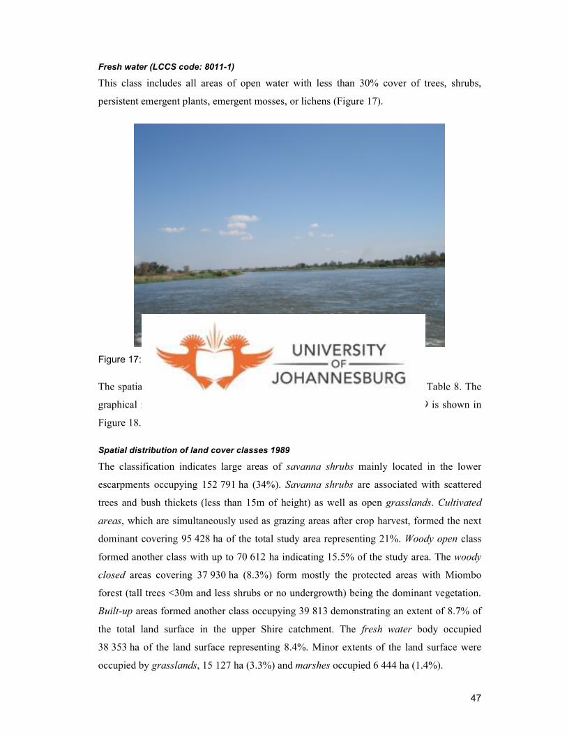
47
Fresh water (LCCS code: 8011-1)
This class includes all areas of open water with less than 30% cover of trees, shrubs,
persistent emergent plants, emergent mosses, or lichens (Figure 17).
Figure 17: Fresh water body
The spatial extents of each land cover type for 1989 and 2002 are shown in Table 8. The
graphical representation of spatial distribution of land cover classes for 1989 is shown in
Figure 18.
Spatial distribution of land cover classes 1989
The classification indicates large areas of savanna shrubs mainly located in the lower
escarpments occupying 152 791 ha (34%). Savanna shrubs are associated with scattered
trees and bush thickets (less than 15m of height) as well as open grasslands. Cultivated
areas, which are simultaneously used as grazing areas after crop harvest, formed the next
dominant covering 95 428 ha of the total study area representing 21%. Woody open class
formed another class with up to 70 612 ha indicating 15.5% of the study area. The woody
closed areas covering 37 930 ha (8.3%) form mostly the protected areas with Miombo
forest (tall trees <30m and less shrubs or no undergrowth) being the dominant vegetation.
Built-up areas formed another class occupying 39 813 demonstrating an extent of 8.7% of
the total land surface in the upper Shire catchment. The fresh water body occupied
38 353 ha of the land surface representing 8.4%. Minor extents of the land surface were
occupied by grasslands, 15 127 ha (3.3%) and marshes occupied 6 444 ha (1.4%).

48
Table 8: Spatial distribution of land cover classes – 1989 and 2002
1989 2002 Class
Area (Ha) Percent Area (Ha) Percent
Fresh water 38 353 8.4 37 178 8.1
Built-up areas 39 813 8.7 14 326 3.1
Cultivated/grazing 95 428 20.9 117 071 25.7
Marshes 6 444 1.4 29 490 6.5
Grasslands 15 127 3.3 63 664 14.0
Savanna shrubs 152 791 33.5 112 356 24.6
Woody open 70 612 15.5 38 446 8.4
Woody closed 37 930 8.3 43 967 9.6
Total 456 498 100 456 498 100
0
50
100
150
200
Fresh water
Built_up areas
Cultivated/graz
Marshes
Grasslands
Savanna shrubs
Woody Open
Woody closed
Area ( 103 Ha)
Figure 18: Land cover extents - 1989
Spatial distribution of land cover classes 2002
The magnitude of the coverage of land surface features for 2002 was slightly different as
graphically portrayed in Figure 19. Among all the land cover classes, cultivated or grazing
areas had the largest extents covering about 117 071 ha (25.7%) of the land surface. The
next large categories included savanna shrubs 112 356 ha (24.6%), grasslands 63 664 ha

49
(14%) and woody closed areas 43 967 ha (9.6%). Woody open represented 38 446 ha
(8.4%) of the study area. Fresh water covered about 37 178 ha totalling 8.1% of the land
surface area and marshes represented 29 490 ha (6.5%). The smallest category was
occupied by built-up areas with 14 326 ha (3.1%) representation.
0
20
40
60
80
100
120
140
Fresh water
Built_up areas
Cultivated/grazing
Marshes
Grasslands
Savanna shrubs
Woody Open
Woody closed
Area (103Ha)
0
20
40
60
80
100
120
140
Fresh water
Built_up areas
Cultivated/grazing
Marshes
Grasslands
Savanna shrubs
Woody Open
Woody closed
Area (103Ha)
Figure 19: Land cover extents - 2002
2.4.4 Distribution of land cover categories
Documenting the distribution of land cover types within the Shire River catchment is the
foundation for applications not only in the study of surface water redistribution and run-off
but also in monitoring environmental trends. The advancement in the capabilities of
Landsat satellite has enabled the measurement of the amount of impervious surface and
vegetation representation with a 30 m pixel in the Shire River catchment. Impervious
surface and vegetation cover distribution can be combined to measure and model
hydrological impacts. Impervious surfaces include all surfaces (fabricated or natural) that
inhibit infiltration by rainfall. Vegetation acts as an integrator of many physical and
biological properties of an area. Characterising the complex cover types created by
variation in vegetation cover proportions provide spatial data that can be used to model
hydrological impacts in the Shire catchment. The classified land cover classes indicate
marked variations in their spatial distribution [Palamuleni et al., 2006].

50
Woody closed
In reference to the altitudinal distribution, this type of forest is mostly confined to the
higher elevations. The majority of woody closed areas constitute the bulk of forested area
in the south east (Machinga Hills), north east (Namizimu forest) and mid north west
(Phirilongwe) regions of the catchment (Figure 20).
Machinga Hills
Namizimu Forest
Phirilongwe Forest
Machinga Hills
Namizimu Forest
Phirilongwe Forest
Figure 20: Location map of forest reserves
Woody closed areas are found mostly in designated forest reserves with dissected rocky
steep escarpment and gorges. Most of the vegetation is associated with shallow and stony
lithosols. These factors are unattractive to subsistence farming and as such, these areas
have not been utilised as much for subsistence cultivation. However, due to increasing
population growth there is increasing land pressure and demand on forest resources. Forest
transitions of shrubs and grasslands dominate the lower and middle sections of the
escarpment especially in areas close to settlements. These changes are discussed further in
Chapter 3.
Also classified as woody closed are Eucalyptus globulus (bluegum), Gmelina aborea
(gmelina) and Acacia nigrescens (acacia) woodlots mainly located in the eastern part of the
study area and within school grounds. Annual tree planting exercises promote planting of
such trees. The woodlots had similar spectral reflectance to woody closed as verified by
field data and site context.

51
Woody open
Apart from forest reserves, which have been mapped as woody closed areas, the woody
open category is found in the lower escarpment and the valley regions within the study
area. Remnants of woody open forests are located in the river valleys, residual hills and
cultivated or grazing areas. The land use practices are the major causes of deforestation
and degradation of this type of forest. Trees of economic importance such as Zizyphus
jujube (masau), Mangifera indica (mango) and Faidherbia albida (msangu) are left on the
cultivated fields and around homesteads.
Savanna shrubs
Savanna shrubs constitute the dry deciduous group, which is more pronounced in the
calcimorphic alluvial terraces of the catchment. Savanna shrubs occur in close association
with grasslands and cultivated or grazing areas class, and are referred to as mopane
woodlands. This category has wider altitudinal distribution than any other class. A majority
of the savanna shrubs are found from 100 m to as high as 800 m above sea level and
commonly distributed in various sections in the catchment.
Grasslands
Continuous tree felling has given rise to open and sometimes patchy grasslands found
almost everywhere in the study region. This class occurs in close association with savanna
shrubs and cultivated fields where grass is left to thrive after harvesting. The grass heights
may range from 1.5 m to 3 m commonly Acacia macrothyrsa often in the well-drained
calcimorphic soils while the short grasses, Chloris gayana (Luba) are found in the eroded
low-lying sites. However, discriminating the different grass species is rather difficult in
remote sensing due to similarity in spectral reflectance. Cattle often graze the short grasses
and the tall grasses are harvested for thatching houses. The grasses are often burned during
the dry season. If grasslands are overgrazed or subjected to uncontrolled burning, patches
of bare ground are created, leading to increased evaporation and accelerated run-off.
Marshes
Seasonally inundated grasslands found along the shores of Lake Malombe and the Shire
River. Field exercise indicated dry season cultivation in the marshes when water levels
were generally very low.

52
Cultivated/grazing areas
During the fieldwork exercise, it was noted that there is a clear indication of continuous
cultivation in most farming areas (Figure 9). Fire is the most commonly used land-clearing
practice, which contributes substantially to the degradation. Because of low yields and
insufficient areas for subsistence cultivation, farmers encroach into neighbouring hills,
which are primarily forests and steep slopes. This is the most damaging form of activity
because such areas are vulnerable to accelerated soil erosion and run-off.
As noted by the Department of Environmental Affairs, people in Malawi and the upper
Shire River catchment in particular, will continue to be dependent on natural resources for
their livelihood in the foreseeable future [Malawi Government, 1998a]. At present, the
country has a large population, which is not yet consumer-oriented, has low energy
consumption, small-scale industrialisation and subsistence pattern of farming without
rotational cycles. However, since subsistence agriculture has low productivity, there has
been an inevitable tendency to increase the amount of land being farmed by using marginal
areas.
Patches of cultivated or grazing areas classified in the Liwonde National Park could be
attributed to misclassification and differences in water level between the two periods.
Built-up areas
Built-up areas in the study area are both clustered and scattered depending on population
densities. Mangochi Township forms the major township located near the source of Shire
River while village settlements are spread throughout the study area. However, detailed
settlement distribution could not be easily mapped due to spectral similarity between
building materials (grass roofing and mud walls) and the surrounding grasslands and
cultivated areas (Figure 16). A detailed discussion of the changes in built-up areas has been
given in Section 3.4
Fresh water
The mapped water bodies are mostly reservoirs and rivers. Water volumes and surface
areas change in response to seasonal and climatic variations. The largest continuous water
body includes Lake Malawi, Lake Malombe and the Shire River. Most of the rivers
flowing from Machinga hills and Phirilongwe forest into the Shire River have continuous
water during the wet season. During the dry season, most of the small rivers have no flow
practically invisible with Landsat 30 m resolution.

53
2.4.5 Thematic accuracy assessment
Accuracy assessment was based on the correlation between ground reference samples
collected during field exercise and the satellite image classification to give an indication of
the overall agreement between ground-truthing data and processed classifications. Based
on the ground truth observations and the classification, the error matrix in Table 9 was
constructed. The overall mapping accuracy was 87%, with individual classes being
mapped at accuracies of above 77% (user), and above 77% (producer).
Some land cover classes presented particular problems for mapping from the imagery.
These problems were overcome using additional data when available [Palamuleni et al.,
2007]. The most significant confusion was between built-up areas and cultivated or
grazing lands. This yielded a user accuracy of 77%. Built-up areas (especially grass-
thatched) and cultivated or grazing areas occur in similar environments and are often in
adjacent or mixed stands. During dry periods when there is little chlorophyll in the
vegetation, grazing causes exposure of soil between remaining vegetation resulting into
similar spectral values making it difficult to distinguish the two classes. To separate these
types, a combination of vector layers of towns and roads, Normalised Difference Built-up
Index (NDBI) and false colour composites were used. From the NDBI, a Boolean image
was created that contained only built-up and barren pixels having positive values while all
other covers had a value of 0 or –254. This technique was reported to be 92% accurate
[Jensen, 2005] whereas in this research a producer accuracy of 83% was attained which is
highly acceptable.
Marshes were often in confusion with woody open and woody closed areas resulting into
user accuracy of 79% and producer accuracy of 77%. This could be attributed to the
phenology of the covers both having high chlorophyll during the dry season. The woody
trees: Zizyphus jujube (masau), Mangifera indica (mango) and Faidherbia albida (msangu)
are in leaf during the dry season. The plausible way to separate them was using the DEM
where marshes are located in very low areas close to water bodies while woody trees are
mostly located in upper areas in association with cultivated areas.
Shrublands and grasslands in the catchment form a complex matrix that is patchy in some
places and homogeneously mixed in others, and spectral separation was difficult. To
separate these types, transformations and contextual knowledge of the area were
incorporated. Digital elevation and soil data helped to identify boundaries between woody

54
open and woody closed areas. The closed woodlands are dominant in hills and plateau
areas while the open woodlands are common in the lower escarpment. From a remote
sensing point of view, discriminating open mixed deciduous with an area cleared under
shifting cultivation or logging activities proved difficult. Because of the dry non-growing
season, the field supposed to belong to cultivation category appeared mostly as shrubland.
The most accurately classified land cover was the fresh water category due to its
contiguous nature that exhibited a unique spectral signature. Fresh water had 100%
accuracy for both producer and user accuracy. The user accuracy of 100% for grassland
could be explained by the fact that the land cover class was broad and large homogeneous
polygons were purposively selected for the exercise.
2.5 Conclusion
The basis of this research comprised multi-temporal classification of Landsat satellite
imagery to provide a recent perspective of land cover types within the upper Shire River
catchment. Results from this study indicate successfully the synergy between Landsat data,
vector data and detailed ground information in mapping land cover features. It was found
that by integrating contextual information and ancillary data, discrimination of
heterogeneous land cover classes dominant in savanna woodlands was improved. Eight
land cover classes were mapped for the Shire River catchment, with an overall accuracy of
87%. Thus, the classification procedure not only separated land cover into different
classes, but also illustrated the patterns that exist across the landscape.
In addition, this project has produced land cover maps at 1:50 000 scale for the Shire River
catchment, covering 4,500 km2. These maps were prepared using Landsat satellite data,
acquired in 1989 and 2002 as the main data source and thus represent the land cover
existing at that time. The land cover maps have compatible digital formats hence they can
easily be applied to a variety of future GIS applications. Additional themes can be
incorporated as more resource information becomes available, or as new management
needs are identified.

55
Table 9: Error matrix for land cover classes
Ground truth data
Classification Fresh water
Built-up areas
Cultivated /grazing
Marshes Grass-lands
Savanna shrubs
Woody open
Woody closed
TR Accuracy
Fresh water 11 0 0 0 0 0 0 0 11 100.0%
Built-up areas 0 20 5 0 0 0 1 0 26 76.9%
Cultivated /grazing 0 2 40 0 1 2 5 1 51 78.4%
Marshes 0 2 0 23 0 0 0 0 25 92.0%
Grasslands 0 0 0 0 29 0 0 0 100 100.0%
Savanna shrubs 0 0 0 0 0 20 2 0 22 90.9%
Woody open 0 0 1 6 0 0 31 1 39 79.5%
Woody closed 0 0 0 1 0 0 0 24 25 96.0%
TC 11 24 46 30 30 22 39 26 228
Total 100% 83.3% 87% 76.7% 96.7% 90.9% 79.5% 92.3%
where TD = sum of major diagonal, TC = column totals, TR = row totals. The overall classification accuracy was TD/TR (198/228) = 87%. Errors were considered consistent with limits of the available technology and ancillary data.

56
The present study has adopted the hierarchical legend structure determined by the Food
and Agriculture Organisation (FAO) Land Cover Classification System (LCCS) to label
land cover variables [Di Gregorio and Jansen, 2005]. LCCS was used as a basis for the
classification to achieve legend harmonisation within Africa and on a global scale.
Currently, the system serves as an internationally agreed reference base for land cover
mapping. LCCS is a relatively new classification system and has been applied in the
Africover project [Di Gregorio and Jansen, 2005]. Through the Africover Programme and
the GLCN initiative, a number of countries were mapped using the LCCS classification
system including: Burundi, Democratic Republic of Congo, Egypt, Eritrea, Kenya,
Rwanda, Somalia, Sudan, Tanzania and Uganda. No land cover mapping study to date has
been conducted in Malawi using LCCS as a coding classification system. The adoption of
LCCS carried out in this research may thus be an important step towards a rigorous update
and translation of the existing land cover maps for Malawi.
The new classification system is also internally consistent, allowing scalability and
mappability that can be used at different scales and levels of detail to discriminate land
cover features. The methodology is applicable at any scale and is comprehensive in the
sense that any land cover identified anywhere in the world can be readily accommodated.
In addition to compatibility with the FAO/LCCS, the derived land cover maps have
provided recent and improved classification accuracy, added thematic detail compared to
the existing 1992 land cover maps.
LCCS presents an advantage for mapping heterogeneous landscapes such as those present
within the Shire River catchment in Malawi. The distributions of savanna woodlands, rural
residential areas, both clustered and scattered (with grass thatched roofing, mud walls and
occasionally iron sheet roofing) and cultivated or grazing areas, represent classes which
have similar spectral signatures (especially during the dry season). They occur in similar
environments and are often in adjacent or mixed stands. Flexibility of LCCS allows
incorporation of geographical data sets to facilitate definition of class boundaries that are
explicit and clear. In this study, digital elevation objects, soil and underlying geological
features were used to identify boundaries between spectrally similar land cover types, for
example, open woodlands and closed woodlands. The closed woodlands are dominant in
hills and plateau areas associated with lithosols while open woodlands are common in the
lower escarpment. Overall, the hierarchical classification technique presents an advantage

57
for mapping heterogeneous landscapes such as those present within the Shire River
catchment.
In terms of classification methodology, the overall approach developed and applied in the
study comprises a variety of techniques ranging from integration of contextual information
such as terrain height and soil characteristics to Maximum Likelihood classifier. The
combination of analytical tools grants considerable insights in land cover mapping of
heterogeneous savanna woodland environments. The approach has the potential of being
adapted and replicated in other similar regions of the world, hence enhancing knowledge of
land cover mapping and dynamic processes at the policy-relevant meso-scale.
The derived land cover maps have added thematic detail enabling spatial and temporal
analysis of patterns and trends in land cover in the upper Shire River catchment. Mapping
of built-up areas was significant as it provided information for establishing the association
between the spreading pattern of the built-up areas with the intensity of cultivation system
and other changes in land cover classes. As such, the characteristically localised nature of
catchment changes can easily be accounted for, making it possible for interpretation and
prediction of the effects of land cover change. These changes are further discussed in
Chapter 3. Results of land cover dynamics reported here will be used as input data for
hydrological modelling in Chapter 4 to establish relationships between fluctuations in the
hydrological regimes and each land cover class.

58
Chapter 3
3 LAND COVER CHANGE ASSESSMENT 1989-2002
Chapter 3 examines of land cover changes in the upper Shire River catchment. Using
Landsat classifications, a discussion of the changes in landscape diversity and
fragmentation between 1989 and 2002 is presented. Areal statistics and the direction
of change in each land cover class were derived. Combination of both image overlay
and post-classification change detection methods reveals significant changes that have
occurred in the Shire River catchment between 1989 and 2002. Changes in land cover
have potential effects on the hydrological processes of the catchment.
3.1 Land cover change
Rapid changes in land cover have a significant impact on conditions of catchment
ecosystems. Accurate information on the status of and trends in land cover changes is
needed to develop strategies for sustainable development and to improve the livelihood of
communities. The ability to monitor catchment land cover changes is highly desirable by
both local communities and policy decision makers. With increased availability and
improved quality of multi-spatial and multi-temporal remote sensing data as well as new
analytical techniques, it is now possible to monitor catchment land cover changes and their
potential hydrological responses in a timely and cost-effective way.
In Malawi, as in many other countries, the landscape is continually changing under the
influence of several factors (including population growth, agricultural expansion and
urbanisation), and as a result, land cover maps rapidly become out of date. In the area
under consideration - the Shire River catchment - two factors may be related to land cover
changes in the past two decades: population growth and the expansion of subsistence
agriculture. Population growth causes changes in land cover through the expansion of
human settlements. The conversion of land to cropland for food security is a cause of
major concern. Forest clearance has resulted from an increased demand for forest products
such as fuelwood, commercial logging and construction materials. Many current land
cover practices in the catchment have the potential to adversely effect and degrade the
environment with respect to forests, soil, water, and biodiversity resources. Previous
studies show increasing land cover change without quantifying the degree and direction of
change in terms of land cover categories [Green and Nanthambwe, 1992]. The impact of
such land cover changes on land surface hydrological processes is of major interest in this
thesis.

59
3.1.1 Land cover change and hydrological response
Land cover plays a critical role in the hydrological cycle, as water availability is generally
a consequence of the distribution of precipitation into evaporation, run-off and soil
moisture storage [Dolman and Verhagen, 2003]. There are many connections between land
surface characteristics and the water cycle. Firstly, land cover can affect both the degree of
infiltration and run-off following precipitation events. Secondly, the degree of vegetation
cover and the albedo of the surface can affect rates of evaporation, humidity levels and
cloud formation. Any change in land cover will have correlated effects in the hydrological
regimes, and possible impacts on the habitat and ecological communities [Calder, 1992;
Lorup et al., 1998].
Agricultural developments have resulted in the widespread deterioration of soil structure, a
process which favours soil sealing and crusting, and related modifications in the rates of
infiltration and storage [Boardman and Favis-Mortlock, 1993; De Roo et al., 2001;
Robinson, 1990]. Specifically enhanced grazing pressure and intensive cultivation
practices have led to soil compaction, reduced infiltration and ground water recharge and
excessive run-off [Boardman and Favis-Mortlock, 1993; Evans, 1990; Forher et al., 2001;
Moussa et al., 2002].
In catchments which were traditionally cultivated or grazing areas that have been changed
to woodland, increases in evaporative loss and decreases in discharge to the outlet have
been observed [Dagnachew et al., 2003; De Roo et al., 2001; Robinson, 1990]. The effect
of land drainage on river discharge can enhance peak flows by increasing the density of
rivers or inhibiting water flow (infiltration) and storage within the soil matrix [Maidment,
1993]. Consequently, seasonal variations in river discharge have been associated with
decreased infiltration during the wet season, which can influence the streamflow during the
dry season by inhibiting ground water recharge.
The consequences of forestation include an increase in infiltration and a reduction of the
incidence of surface run-off influencing the seasonal regime of rivers. However,
infiltration generally depends upon the combined effect of soil properties, climatic
conditions as well as land cover and the developmental stage of the vegetation.
Demonstrations from catchment studies showed that the pine forestation of former
grassland not only reduces annual streamflow by 440 mm but also reduces the dry season
flow by 15 mm [Bosch, 1979]. Thus, benefits gained by the forestation of degraded or
eroded catchments will be dependent on the situation and the management methods
employed [Calder, 1998].

60
Various microclimate changes resulting from land cover changes have been documented.
Deforestation alters the disposition of radiant energy by increasing surface albedo and
daytime long-wave emission by the land surface resulting in lower net radiation [Bastable
et al., 1993; Culf et al., 1995; Larkin, 2002]. The characteristics and variable state of the
land surface control the proportions of net radiation extended upon latent
evapotranspiration and sensible energy flux. A drastic change in vegetation cover, such as
clear cutting in the Pacific north-west, can produce 90% more run-off than in catchments
unaltered by human practices [Franklin, 1992]. Replacing forests with other land cover
types changes the energy partitioning because of differences in leaf area, aerodynamic
roughness, root depth, and stomata behaviour. Field studies have verified that the
replacement of forest by pasture or non-irrigated crops reduces evapotranspiration which
generally increases streamflow, possibly increasing flood hazards [Giambelluca et al.,
2000; Jipp et al., 1998; Wright, 1992]. However, as Bruinjzeel [2001] emphasises, the
effects of deforestation on evapotranspiration and streamflow are not uniform, and depend
on the original forest type, characteristics of replacement land cover, climate, exposure and
soil depth.
Canopy characteristics such as canopy depth, crop height and spacing, leaf area and shape
will have an influence on the hydrological performance of vegetation cover through its
effects on interception. Studies conducted in wet conditions [Bouten et al., 1991] indicate
that interception losses will be higher from forests than from shorter crops resulting in the
reduction of run-off from forested areas compared with those under shorter vegetation. In
addition, the amount of vegetation controls the partitioning of incoming solar energy into
sensible and latent heat fluxes thereby affecting evapotranspiration rates. Yet in deforested
areas, interception and evaporation rates will be lower while increasing surface run-off and
sediment production which consequently lower flow discharge to rivers [Calder, 1992;
Newson, 1992; Shaw, 1990]. However, the amount of precipitation intercepted and
evaporated will vary depending on the vegetation type and species [Hall and Calder,
1993].
Land cover conversions such as the change from forests or vegetated areas into urban land
uses have many hydrologic effects with significant ecological and sociological
ramifications [Booth, 1991; Hollis, 1975; Leopold, 1968]. These changes reduce
interception, infiltration, subsurface flow, evapotranspiration, storm water storage on hill

61
slopes, and the time required for storm water to travel over and through a hill slope to a
stream [Burges et al., 1998; Dinicola, 1990]. The percentage of the catchment surface that
is impermeable due to urban and road surfaces influences the volume of water that runs
and increases the amount of sediment that can be moved [Arnold and Gibbons, 1996].
Urbanisation is known to transform permeable areas such as forest and farmland into
impermeable areas, thereby reducing the amount of water infiltrated into the soil and the
amount of water on the ground surface [Cheng and Wang, 2002; DeFries R. and
Eshleman, 2004]. As run-off volumes in urban channels increase, the duration of high flow
decreases because groundwater is no longer contributing to the flow. In addition, urban
development causes a decrease in lag time between rainfall and run-off by increasing the
hydraulic efficiency of the drainage system (water can reach the channel more swiftly
when it travels over smooth, hard surfaces). In addition, in urban areas, which are largely
covered by roads and buildings, water evaporation from the ground surface and plants into
the atmosphere is generally lower than in agricultural areas or forests. Recent results
regarding the impact of land cover change on hydrological regimes in urban areas have
been discussed elsewhere [Acreman et al., 2000; De Roo et al., 2001; Jennings and
Jarnagin, 2002; Lahmer et al., 2001]. Theoretically, urban built-up areas - especially those
with impervious surfaces - could affect the flow behaviour within a catchment.
The size of a catchment will also influence the hydrological response of precipitation
where small catchments show obvious responses to specific land uses. In large catchments,
meanwhile, hydrological responses are affected by the complex water storage and release
mechanisms [Calder, 1992; Forher et al., 2001]. In small catchments, land use changes to
urbanisation will reduce evapotranspiration and infiltration and increase surface run-off
[De Roo et al., 2001]. Land use change to forest will increase evaporation which may
result in low soil moisture and possibly increase infiltration during rainfall resulting in a
decreased run-off [Calder, 1992; Dagnachew et al., 2003; De Roo et al., 2001]. However,
management activities associated with forestry such as cultivation, drainage, road
construction and soil compaction during logging are more likely to influence hydrological
responses than the presence or absence of the forests themselves.
The magnitude of land cover effects will be dictated by the nature and scale of the land
cover change. This is also linked to physiographic, climatic and management differences.
Land cover change studies should be viewed as responding to the complex interactions and
62
feedbacks linking social, or indirect and direct biophysical processes that occur on the land
[Dolman and Verhagen, 2003; Maidment, 1993]. To balance the supply and demand for
water resources and to reduce negative or undesired effects for the environment and
society, changes in actual land cover have to be studied at all spatial scales due to the
heterogeneous patterns of the distribution of terrestrial vegetation and soils over land
surfaces [Verburg et al., 1999]. Therefore, establishing clear linkages between specific
land cover changes and hydrological responses at the catchment scale poses a challenging
problem in hydrological studies.
3.2 Land cover change detection
The use of multi-date satellite remote sensing data to detect land cover change began in the
early 1970s [Singh, 1989]. Change detection is the process of identifying differences in the
state of an object or phenomenon by observing it at different times [Singh, 1989]. The
process encompasses the quantification of multi-date imagery to derive changes over two
time periods [Coppin et al., 2004]. It is an important process in monitoring and managing
natural resources and urban development because it provides a quantitative analysis of the
spatial distribution of the population of interest. Change detection is useful in such diverse
applications as land cover change analysis, the monitoring of shifting cultivation, the
assessment of deforestation, the study of changes in vegetation phenology, seasonal
changes in pasture production, damage assessment, crop stress detection, disaster
monitoring, day/night analysis of thermal characteristics as well as other environmental
changes [Singh, 1989].
Techniques to perform change detection with satellite imagery have become numerous as a
result of the increasing versatility of digital data and increasing computing power. A wide
range of approaches to change detection analysis have been reported [Fung, 1990; Green et
al., 1994; Howarth and Wickware, 1981; Jensen, 1986; Jensen et al., 1993; Lillesand et al.,
2004; Milner, 1988; Mouat et al., 1993; Singh, 1989]. Approaches include transparency
compositing [Crapper and Hynson, 1983], image differencing [Dale et al., 1996;
Muchoney and Haack, 1994; Price et al., 1992], image ratio-ing, classification
comparisons [Dale et al., 1996; Jensen, 1995; Muchoney and Haack, 1994], image
enhancement techniques, such as principal component analysis [Fung and LeDrew, 1987],
Normalized Difference Vegetation Index [Mikkola, 1996], image algebra change detection
[Green et al., 1994], and post-classification comparison [Rutchy and Vilchek, 1999].

63
Although these methods have been successful in monitoring change for a myriad of
applications, there is no consensus as to the ‘best’ change detection approach. The type of
change detection method employed is largely dependent on the purpose of the change
investigation, data availability, the geographic area of study, time and computing
constraints, and the type of application [Coppin et al., 2004].
Rather than attempt to review all published change detection techniques, only techniques
that have been selected for use in this study are reviewed, namely image overlay and post-
classification analysis. The purpose of change detection in this exercise is focused on
factors that may influence the behaviour of the hydrological regimes in the catchment.
Image overlay
This change detection algorithm uses a digital enhancement technique for on-screen
change delineation. It provides a simple mechanism to display changes between two dates
of imagery quickly and efficiently [Jensen, 2005]. The image is prepared by making a
photographic two-colour composite showing the two dates in separate colour overlays. The
colours of the resulting image indicate changes in reflectance values between the two
dates. For instance, features which are bright (high reflectance) on date one, but dark (low
reflectance) on date two, will appear in the colour of the first photographic overlay and
vice versa. Features which are unchanged between the two dates will be equally bright in
both overlays and hence will appear as the colour sum of the two overlays.
To represent the bi-temporal variations within one single image product, Alwashe and
Bokhari merged TM bands 2, 4, and 5 of two different acquisition dates via an intensity-
hue-saturation (IHS) transformation. On such an image, vegetation differences showed up
in distinctly different colours [Alwashe and Bokhari, 1993]. Similarly, Sunar [1998]
performed change detection between Landsat TM data of 1984 and 1992 and observed that
areas of no change were represented by values of 127 (mid-grey), while areas that were
darker in 1992 than they were in 1984 had values between 128 and 255. However, this
technique provides the analyst with little information regarding the nature of the change
[Jensen, 2005].
Post-classification analysis
Post classification analysis is the most commonly used method of land cover change
detection. It is a comparative analysis of spectral classifications for times t1 and t2 (or
more) produced independently [Singh, 1989]. Classification results are compared on a

64
pixel-by-pixel basis using a change detection matrix, and the areas of change extracted
[Jensen, 1996; Jensen, 2005; Singh, 1989; Yuan and Elvidge, 1998]. The classified images
are combined to create a new change image classification. The new image indicates the
changes “from” and “to” that took place and the kind of landscape transformations that
have occurred are calculated and mapped. The advantage of this method includes the
detailed “from-to” information that can be extracted. Individual classification of two image
dates minimises the problem of normalizing for atmospheric and sensor differences
between two dates [Jensen, 2005; Singh, 1989] although accurate geo-referencing and
accurate classifications are crucial to ensure precise change-detection results [Augenstein et
al., 1991; Foody, 2001; Rutchy and Vilchek, 1999].
A useful example of the use of the post-classification approach is the work of Munyati
[2000] in which Landsat images acquired in 1984, 1988, 1991 and 1994 were used to
assess change on a section of the Zambian Kafue Flats floodplain wetland system. Similar
supervised Maximum Likelihood classification procedures were employed on all images.
The classified images produced were analysed for change in each land cover category by
overlaying them in a GIS framework, and transition rates between the classes were
calculated. The change detection results provided a reliable indication of the long-term
change that the Kafue Flats wetland area has undergone.
Land cover maps derived from Landsat 5 and Landsat 7 ETM+, discussed in Chapter 2,
form the input data for change detection. Two approaches were used to detect changes in
the upper Shire River catchment, namely image overlay and post-classification analysis
and their results compared. Using image overlay, vegetation characteristics were chosen as
the main indicator of land cover change. Post classification statistical analysis was
employed to determine the specific nature of changes between dates of imagery (1989 and
2002) in each land cover class. Image overlay was found to detect areas of change and no
change within the catchment. By using post classification procedures, areal statistics and
the direction of change in each classified land cover class were derived. A combination of
both methods reveals the significant changes that have occurred in the Shire River
catchment between 1989 and 2002. These activities also highlighted areas where there are
major changes in land cover (i.e. "hot spots"), in both temporal and spatial aspects.

65
3.3 Methodology
3.3.1 Input for change detection
Land cover maps derived and discussed in Chapter 2 form the basis of data for the land
cover change detection.
3.3.2 Approaches
Image overlay
In this approach, vegetation reduction was chosen as the main indicator of land cover
change. Therefore, band 4 of Landsat TM and ETM+ (near-infrared) respectively were
selected. For the 1989 image, band 4 was displayed through the R and B (blue) channels of
the computer monitor. Band 4 of the 2002 image was displayed through the G (green)
channel of the computer monitor. This technique is not intended to be quantitative but
rather was used to identify qualitatively and explore the areas of change in the Shire River
catchment.
Post-classification
The starting point for the post-classification approach is a pair of images for which land
cover classification and labelling have been carried out, in this case the Landsat TM and
Landsat ETM+ images discussed in Chapter 2. The next step is to compare the resultant
classification images on a pixel-by-pixel basis and to extract areas of change using a
change detection matrix. A change detection matrix is an {N x N} table of change
detection classification codes produced by assigning a unique integer to each possible
change from one land cover category to every other category, where N is the number of
thematic land cover classes in the study.
For this study, eight land classes were identified. Each of the eight identified land classes is
assigned a base value in the sequence {20, 40 …160}. A 64-cell table (8 x 8) of change
detection codes, was created for each possible pair of “changed from” and “changed to”
combinations by incrementing a base value by unity, e.g. from the base value 20 assigned
to built-up areas, the vector {21, 22 …28} is created. The full set of assigned codes is
presented in Table 10. A change from savanna shrubs to built-up areas, for example,
would be represented by the code 26 shown in column 1. Diagonal elements of the matrix
are assigned to pixels that have not undergone change. Certain changes are physically
improbable, e.g. open water to woody closed, but values are assigned to complete the
matrix.

66
By applying these change detection codes to the comparison of the two classified images, a
new layer is produced, the post classification change layer, with each pair of pixels
represented by a change detection code. From the change detection layer, change detection
maps may be produced to visualise areas of change by assigning colours to single or
grouped categories of change. For example, any pixel in the 1989 map that changed to
built-up area by 2002 is assigned the value red; any pixel that changed into cultivated or
grazing land by 2002 is assigned the value pink. The assigned colours to be used in the
results section are superimposed on the matrix shown in Table 10.
Table 10: Assignment of Change Classification Codes of land cover for the Shire River
Catchment for 1989 and 2002
Built-up areas
Cultivated/grazin
g
Fresh Water
Grass-lands
Marshes Savanna shrubs
Woody open
Woody closed
To 2002
From 1989 20 40 60 80 100 120 140 160
Built-up areas 21 41 61 81 101 121 141 161
Cultivated/grazing 22 42 62 82 102 122 142 162
Fresh water 23 43 63 83 103 123 143 163
Grasslands 24 44 64 84 104 124 144 164
Marshes 25 45 65 85 105 125 145 165
Savanna shrubs 26 46 66 86 106 126 146 166
Woody open 27 47 67 87 107 127 147 167
Woody closed 28 48 68 88 108 128 148 168
� no change in land cover between dates � new built-up areas � land cover change to cultivated or grazing areas � water related changes not selected for display � water � change in land cover to vegetated areas � vegetation regeneration from previously built-up areas � land cover change to grassland areas � change in land cover to vegetated areas
This table is interpretable by presenting tabular results quantifying change between classes,
such as the change from woody open to cultivated or grazing land. The table shows the
degree of change, the pixel prior classification, and the pixel post classification. This
matrix can be used to distinguish the entire change analysis in one view and is thus a
powerful tool for examining landscape change.

67
Land cover change areal statistics were also summarised to express the net land cover lost
and gained by each class. This was accomplished by subtracting the total amount of land
cover gain from the total amount of loss. Statistics were compiled in the Microsoft Excel
programme to determine the specific nature of changes between dates of imagery, i.e. the
size of the differences between the dates and the direction (positive and negative) in each
land cover type.
3.4 Results and discussion
3.4.1 Image overlay
The visual overlay composite image (Figure 21) indicates visual changes in land cover
change that took place in the upper Shire River catchment between 1989 and 2002. This
image highlights the changes in vegetation and qualitatively assesses the extent of the
change. This technique showed clearly areas of no change, and areas where changes have
taken place, in the upper Shire River catchment. The resulting image is grey in areas where
no change has occurred, such as to the west of the Shire River in the Liwonde National
Park. Where vegetation has decreased, the image is magenta/purple and where vegetation
has increased, it is green.
In Figure 21, the magenta regions represent vegetation that has been cleared for new
cultivation and settlements. Major vegetation reductions are apparent within Mangochi
Township near the outlet of the Shire River (Figure 22).
Mangochi is one of the fastest growing towns in Malawi due to the development of tourism
around the Shire River and Lake Malawi [National Statistical Office, 2000]. Its population
had increased from 496 578 in 1987 to 599 935 in 1998 as captured by population censuses
[National Statistical Office, 2000]. The high population growth has translated into rapidly
increasing demands from land in terms of food, shelter, energy (in particular, fuelwood)
and construction materials. Disappearing vegetation cover lessens the landscape's ability to
intercept, retain and transport precipitation. Instead of trapping precipitation, which then
percolates to groundwater systems, deforested areas become sources of surface water
run-off, which moves much faster than subsurface flows.

68
Figure 21: Image overlay for the Shire River catchment: 1989 — 2002

69
Mangochi TownshipMangochi Township
Figure 22: Expansion of Mangochi Township into previously vegetated areas
Another area of interest is the riverline below Lake Malombe, which shows a decreasing
trend in marshes, in contrast to an increase of marshland above the lake. Marshes are
critical because they recharge groundwater supplies and moderate streamflow. This is an
especially important function during periods of drought. The presence of marshes in a
catchment helps to reduce damage caused by floods by slowing and storing flood water. It
was verified during the field exercise (Section 2.3.2) that the grass-covered marshes have
either been drained and cultivated or overgrazed. These agricultural activities are part of an
initiative by Save the Children (UK), a non-governmental organisation, as a means of
increasing food security in the area.
In some parts of the south-eastern and north-western side of the catchment, some degree of
vegetation recovery is depicted. These areas were previously occupied by Mozambican
refugees during the civil war between 1976 and 1992. After the civil war ended, most
refugees returned to Mozambique. The harvesting of natural forest products by the
occupants of these refugee camps resulted in significant loss of forest area and increase in
fragmentation as captured by the 1989 image. By 2002, vegetation re-growth can be
observed in most of what were previously refugee camps. The green regions represent

70
higher reflectance in the near-infrared wavelength signifying vegetation re-growth through
natural processes and government intervention through reforestation programmes. At the
initial stage of the reforestation programmes, exotic trees such as bluegum and gmelina
were planted. However, water resources were being compromised due to these fast
growing species. The Malawi Government and NGOs working in this area, now
rehabilitate the camps with indigenous trees [Kafakoma, 1996]. As a result, the presence of
vegetation can change the quantity of water on the surface, in the soil or groundwater
recharge. This in turn affects run-off rates and the availability of water for either ecosystem
functions or human services.
3.4.2 Post classification and land cover change areas
Results from post-classification analysis are presented using a series of change maps for
visualisation, and statistical tables to provide quantitative measures of change. The change
maps use the colour coded from-to indices of change defined in Table 10.
Change Map
A map of overall land cover changes that have occurred within the Shire River catchment
is shown in Figure 23. The change information is overlaid onto the 2002 Landsat natural
colour image {3, 2, 1} for orientation purposes. Shades of bright green depict areas that did
not change between 1989 and 2002. Areas that have changed to cultivated or grazing lands
are shown in purple. Changes from other types of land cover to vegetated areas are
displayed in yellow and green. This map confirms the qualitative changes indicated in the
change overlay image of Figure 21.
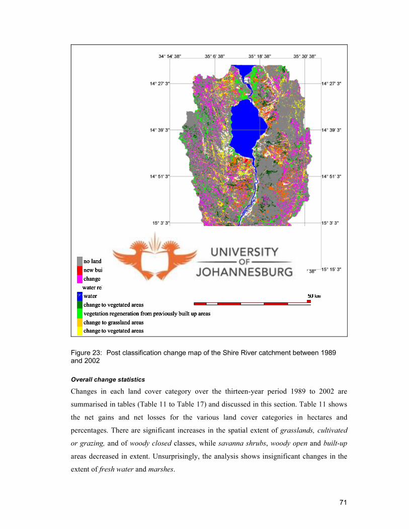
71
no land cover change
� new built up areas
� change cultivated or grazing areas
�water related changesnot selected for display
??� water
� change to vegetated areas
vegetation regeneration from previously built up areas
� change to grassland areas
� change to vegetated areas
no land cover change
� new built up areas
� change cultivated or grazing areas
�water related changesnot selected for display
??� water
� change to vegetated areas
vegetation regeneration from previously built up areas
� change to grassland areas
� change to vegetated areas
no land cover change
� new built up areas
� change cultivated or grazing areas
�water related changesnot selected for display
??� water
� change to vegetated areas
vegetation regeneration from previously built up areas
� change to grassland areas
� change to vegetated areas
Figure 23: Post classification change map of the Shire River catchment between 1989 and 2002
Overall change statistics
Changes in each land cover category over the thirteen-year period 1989 to 2002 are
summarised in tables (Table 11 to Table 17) and discussed in this section. Table 11 shows
the net gains and net losses for the various land cover categories in hectares and
percentages. There are significant increases in the spatial extent of grasslands, cultivated
or grazing, and of woody closed classes, while savanna shrubs, woody open and built-up
areas decreased in extent. Unsurprisingly, the analysis shows insignificant changes in the
extent of fresh water and marshes.

72
Table 11: Land cover changes of the Shire River catchment during 1989 to 2002
Total area in land
class at 1989 ( ha )
Total area changed to per class
(ha)
Total area changed from per land class
(ha)
Net gain (loss) (ha)
Net change (%)
Built-up areas 39 813 456 2 005 -1 549 -3.9
Cultivated or grazing
95 428 4 622 3 158 1 464 1.5
Fresh water 38 353 0 108 -108 -0.3
Grasslands 15 127 3 616 469 3 147 20.8
Marshes 6 444 108 180 -72 -1.1
Savanna shrubs 152 791 2 584 4 370 -1 786 -1.2
Woody open 70 612 1 312 3 017 -1 705 -2.4
Woody closed 37 930 1 652 1 043 608 1.6
Total area 456 498 14 350 14 350 0
Changed areas for each land cover type are calculated by summing the respective numbers
of from-to change pixels occurring in the change detection matrix for each change
classification code (Table 10). Reference is made to the changed land area of the
catchment (excluding water bodies) amounting to 14 350 ha. The entire catchment
excluding open water bodies is 418 145 ha, thus the total changed area represents 3.43% of
the land area of the catchment. The following sections discuss changes within each land
cover class.
Cultivated or grazing areas
The total land area within the upper Shire catchment that was converted from various
classes to cultivated or grazing land amounted to 4 622 ha (Table 12). The increase in
cultivated or grazing land occurred mainly at the expense of savanna shrubs, woody open
areas and built-up areas: cultivated or grazing areas expanded by 1 671 ha (1.0%) from
previously savanna shrubs region; and 1 359 ha (1.9%) from previously woody open areas.
Surprisingly, there is a significant change from built-up areas (1 156 ha) to cultivated or
grazing land.

73
Table 12: Areas changed into cultivated or grazing areas between 1989 and 2002
From Total area in land class at 1989
( ha )
Area changed to cultivated ( ha )
% change
per class♣♣♣♣
Built-up areas 39 813 1 156 2.9
Grasslands 15 127 153 1.0
Marsh 6 444 24 0.4
Savanna shrubs 152 791 1 672 1.0
Woody open 70 612 1 359 1.9
Woody closed 37 930 259 0.7
Total 322 717 4 622 1.4
♣ Percentages calculated as fraction of the original area of the class.
The expansion of cultivated or grazing land indicates increased subsistence agriculture.
Savanna shrubs have experienced degradation and exploitation due to cultivation and
demand for wood resources. The rich calcimorphic alluvial soils render the savanna more
vulnerable to agricultural expansion. Most of the soils in the Shire rift valley are of alluvial
origin, rich in nutrients and ideal for agricultural production. The 2002 land cover map
shows that most of the remaining savanna shrubs are found in the Liwonde National Park
(protected area) and south east of Lake Malombe, which is sparsely populated (Figure 24).
A study of the two classification images shows that cultivated or grazing areas are also
expanding from the lowlands into the higher areas predominantly occupied by woodlands.
These processes are closely related to increases in the demand for food production.
Inevitably, cultivation and encroachment for exploitation of wood for construction and
fuelwood has spread onto such areas as can be noted from the 1989 compared to the 2002
land cover map. This has given rise to a transition from closed savanna woodlands to open
and sparse savanna, and it is mostly economic shrubs that are left in the fields (Figure 24).

74
1989
2002
1989
2002
Figure 24: Expansion of cultivated or grazing areas into predominantly savanna areas
An interesting result is the loss from built-up areas amounting to 1 156 ha which was
converted to cultivated or grazing land. Overall, this represents a net loss of -1 549 ha
(-3.9%) into other land cover categories (Table 11). Built-up areas (especially grass-
thatched) and cultivated or grazing areas occur in similar environments, often in adjacent
or mixed stands and have similar spectral signatures. The decrease could be an aspect of
misclassification due to similarity between roofing materials and the surrounding pixels
dominated by shallow soils and rock outcrops.
Additionally, the ravages of civil war in Mozambique had left large scars on the landscape,
particularly in the forest areas of the eastern mountains, which form the international
boundary between Malawi and Mozambique (Figure 25). Some bare patches where once
there were refugees camps have not yet been reforested, as can be seen in the 2002 image.
These bare patches from dismantled refugee camps are indistinguishable from fallow
cultivated fields and have probably been classified as change to cultivated or grazing areas.

75
Declining forest cover poses serious threats to water supplies within the area. A cause of
concern for this trend in land cover conversion is the significant role the forest reserves
play in catchment management. The forest reserves, Namizimu forest and Machinga hills
(Figure 20) serve some of the big rivers flowing into the Shire River. Overexploited
forestlands are threatened by accelerated run-off and soil erosion, and consequently
degrade the agricultural productivity of the land. Unless monitored, this trend may impact
negatively on the livelihoods of people and the survival of other natural resources in this
area, including water.
Machinga Forest
Namizimu Forest
Forest fragments Machinga Forest
Namizimu Forest
Forest fragments
Figure 25: Forest fragmentation around forest reserve areas
The predominant subsistence agricultural practices signify a gradual but chronic
degradation of the landscape along the valleys and adjoining slopes. These findings concur
with the observations by Kalipeni [1996], which indicates that pressures on land are
increasing, resulting in cultivation of marginal land, more fragile soils and steeper slopes.
Grasslands
From the post-classification land cover change results, 3 616 ha of land was lost from other
classes and converted to grasslands (Table 13). Taking into account losses of grasslands to
other types, the results in a net gain of 3 147 ha (+20.8%) in the extent of grasslands

76
(Table 11). High proportions of change originated from savanna shrubs (1 368 ha) and
cultivated or grazing lands (1 073 ha). Other changes include transition from woody open
land (553 ha), built-up areas (439 ha) and woody closed (158 ha). This is a considerable
change, in view of the short period over which the land cover changes have occurred.
Table 13: Areas changed into grassland areas between 1989 and 2002
From Total area in land class at 1989
( ha )
Area changed to grasslands
( ha )
% change
per class♣♣♣♣
Built-up areas 39 813 439 1.1
Cultivated or grazing 95 428 1 073 1.1
Marshes 6 444 25 0.4
Savanna shrubs 152 791 1 368 0.9
Woody open 70 612 553 0.8
Woody closed 37 930 158 0.4
Total 403 018 3 616 0.9
♣ Percentages calculated as fraction of the original area of the class.
The increase in grasslands from previously woody closed, woody open and savanna shrub
areas is a result of grass thriving best without canopy cover. Increasing demand for wood
resources places substantial strain on landscape integrity. However, the loss of built-up
areas to grassland could be a result of misclassification where the rural building materials
are from dry grass yielding similar spectral response to the natural grassland. In addition,
the surrounding pixels are made of bare soil, which increases the uniformity of spectral
appearance. As a result, spectral classification would assign all pixels including
grasslands, built-up areas and bare soil as a single class.
Changes in fire frequency and timing are known to transform vegetation structure and
composition. Frequent late dry season fires eventually transform woodland into open
grasslands with only isolated, fire-tolerant canopy trees, scattered understory and shrubs
[Desanker et al., 1997]. As the landscape becomes altered, run-off velocity and flow rates
in river systems are also affected.
Savanna shrubs
By analysing the changes that occurred to the landscape, a total of 2 586 ha (0.9%) was
converted to savanna shrub (Table 14). This increase does not compensate for the loss of

77
savanna shrubs to cultivated or grazing areas as discussed above. However, it could be a
result of misclassification as savanna shrubs and cultivated or grazing areas occurring in
similar environments.
Table 14: Areas changed into savanna shrubs areas between 1989 and 2002
From Total area in land class at 1989 ( ha )
Area changed to savanna shrubs ( ha )
% change
per class♣♣♣♣
Built-up areas 39 813 217 0.5
Cultivated or grazing 95 428 1 373 1.4
Grasslands 15 127 267 1.8
Marshes 6 444 32 0.5
Woody open 70 612 377 0.5
Woody closed 37 930 320 0.9
Total 265 354 2 586 0.97
♣ Percentages calculated as fraction of the original area of the class.
Built-up areas
Spatial extents in built-up areas show an overall subtle increase in settlements. Changes in
this land cover category are shown in Table 15 depicting higher land cover changes from
woody open areas (127 ha), cultivated or grazing areas (187 ha) and savanna shrubs
(87 ha). A detailed examination of built-up areas category across the catchment revealed
four important subclasses of change, which are discussed below.
Table 15: Areas changed into built-up areas between 1989 and 2002
From Total area in land class at 1989 ( ha )
Area changed to built-up areas ( ha )
% change
per class♣♣♣♣
Cultivated or grazing 95 428 187 0.47
Grasslands 15 127 28 0.18
Marshes 6 444 7 0.11
Savanna shrubs 152 791 87 0.06
Woody open 70 612 123 0.17
Woody closed 37 930 25 0.06
Total 378 322 457 0.12
♣ Percentages calculated as fraction of the original area of the class.
The spatial distribution of change in built-up areas is of particular interest in this thesis.
Most of the emerging towns, for example Liwonde Township, Mangochi Township and
Balaka Township portray an increase in built-up area signifying an aspect of rural-urban

78
migration (Figure 26). With the national annual urbanisation growth rate estimated at 6.7%
in 1998, many rural dwellers are migrating to urban and expanding district centres in
anticipation of wage employment [National Statistical Office, 2000]. There is a sparse
distribution of spontaneous rural settlements on the lower escarpments, across valleys and
flat lands. With the increasing population, slight expansions into the higher escarpment are
visible on the change image.
Mangochi Township
Built up areas
Mangochi Township
Built up areasBuilt up areas
Figure 26: Built-up areas expanding around Mangochi Township
A decrease in built-up areas is apparent in areas especially formally occupied by
Mozambican refugees. Most of the refugee camps were located to the north western part of
the study area around Mangochi district and Namwera Township. This area is close to the
border with Mozambique such that in 1989 during the civil war most refugee camps had
occupied this area. However, by 2002 the civil war was over and upon the repatriation of
Mozambican refugees, the Malawi Government embarked on land rehabilitation at the

79
former refugee camps, which has resulted in the slight increase of woody closed areas
(Figure 27).
Woody closed areasWoody closed areas
Figure 27: Increase in woody closed areas
Another note of significance is the effects of the electric fence constructed around Liwonde
National Park, a government reserved area, between 2002 and 2004. During the time of the
satellite observation in 1989, there were built-up areas (settlements) close to Liwonde
National Park. Due to prowling animals from the park, many settlements were abandoned,
leading to the regeneration of savanna shrubs as seen in the 2002 image (Figure 9). Field
observations and consultation with members of the surrounding community (in 2006)
indicated that since the containment of animals by the game fence, people have started
moving back to areas close to the park boundary [Palamuleni et al., 2008]. The area is
endowed with calcimorphic alluvial soils, which are very attractive for subsistence farming
(Figure 28).
The boundaries of the reserved area are assumed not to have changed, though subtle
increases in built-up areas do occur within the reserve. These negligible changes are due to

80
the expanding tourism industry within Liwonde National Park, which are visible in Figure
28. New built-up areas along the rivers are primarily composed of tourist resorts and camp
sites.
Liwonde National
Park
Tourist resorts and camp sites
Built up areas expanding outside Liwonde National
park
Tourist resorts and camp sites
Built up areas
Liwonde national park boundary
Liwonde National
Park
Liwonde National
Park
Tourist resorts and camp sites
Built up areas expanding outside Liwonde National
park
Tourist resorts and camp sites
Built up areas
Tourist resorts and camp sites
Built up areas expanding outside Liwonde National
park
Tourist resorts and camp sites
Tourist resorts and camp sites
Built up areas expanding outside Liwonde National
park
Tourist resorts and camp sites
Built up areas
Liwonde national park boundary
Figure 28: Increase in built-up areas and tourism expansion around Liwonde National Park
According to the image classification, the size of built-up areas has decreased between
1989 and 2002 with a net loss of -1 549 ha (-3.9%) into other land cover categories (Table
11). The decrease could be a result of misclassification because the population increased
from 1 011 843 in 1987 to 1 218 177 in 1998 as recorded by population censuses [National
Statistical Office, 2000] and population increases result in the expansion in built-up and
cultivated areas. The misclassification may be a result of local building materials, which
include grass (thatching) and sand (hand made clay bricks) such that built-up areas and
cultivated or grazing areas where there is little green grass and significant exposed soils
are spectrally identical. During summer, most of the areas are non-vegetated with exposed
soils due to ploughing by farmers in preparation for the next crop season. This condition
yields similar spectral values to those of cultivated areas; grass thatched houses and

81
exposed bare areas. Another plausible explaination could be increase in cluster and
nucleated settlement pattern as opposed to scattered settlements.
Percentage of the catchment surface that is impermeable due to settlement and road
surfaces influences the volume of water that runs and increases the amount of sediment
that can be moved [Arnold and Gibbons, 1996]. Generally, such trends in the landscape
could significantly alter the hydrology of the system.
Woody open
A total land area of 1 312 ha (0.38%) was converted from other land cover categories to
woody open land (Table 16). The transitions to woody open areas originated from land
areas previously occupied by marshes (455 ha), cultivated or grazing areas (377 ha),
woody closed areas (281 ha) and built-up areas (166 ha). Although this was a positive
trend, the extent of the transition from for example cultivated or grazing areas (377 ha) to
woody open areas was negligible in comparison to the 1 359 ha loss of woody open areas
to cultivated or grazing areas.
Table 16: Areas changed into woody open areas between 1989 and 2002
From Total area in land class at 1989
( ha )
Area changed to woody open
( ha )
% change
per class♣♣♣♣
Built-up areas 39 813 166 0.42
Cultivated or grazing 95 428 377 0.39
Grasslands 15 127 12 0.08
Marshes 6 444 455 0.30
Savanna shrubs 152 791 21 0.33
Woody closed 37 930 281 0.74
Total 347 533 1 312 0.38
♣ Percentages calculated as fraction of the original area of the class.
Classification errors could be attributed to this transition, which may not be a true
indication of the actual trends in this land cover category. Marshes, woody closed and
woody open areas have similar spectral characteristics as they both have high chlorophyll
during the dry season. The woody trees: Zizyphus jujube (masau), Mangifera indica
(mango) and Faidherbia albida (msangu) are in leaf during the dry season whereas
marshes are mostly evergreen due to presence of water throughout the year.

82
Woody closed
There was a slight increase of 1 652 ha (0.48%) in the area of the woody closed areas
(Table 17). A unique aspect observed in this land cover class is the reclamation of areas
previously occupied by Mozambican refugees and reforestation of school compounds. This
process is illustrated by regeneration from fallow fields especially those areas formerly
occupied by the Mozambican refugees in 1989 (Figure 27). Additionally, annual tree
planting exercises involve the planting of both indigenous and exotic trees such as
Eucalyptus globulus, Gmelina aborea and Acacia nigrescens in woodlots around schools.
As a result, there is a net gain of 608 ha (+1.6%) in woody closed areas across the
catchment area (Table 11). The woodlots had a similar spectral reflectance to the woody
closed areas as verified during field data collection and site context (Section 2.4.5).
Table 17: Areas changed into woody closed areas between 1989 and 2002
From Total area in land class at 1989
( ha )
Area changed to woody closed
( ha )
% change
per class♣♣♣♣
Built-up areas 39 813 28 0.1
Cultivated or grazing 95 428 149 0.2
Grasslands 15 127 10 0.1
Marshes 6 444 70 1.1
Savanna shrubs 152 791 789 0.5
Woody open 70 612 606 0.9
Total 347 533 1 652 0.5
♣ Percentages calculated as fraction of the original area of the class.
The proportion of rainfall that directly reaches the ground surface is affected by the
coverage of vegetation cover. Tree root systems hold the soil together and thus slow the
rate of run-off and reduce erosion. Trees also absorb water during the rainy season.
Because of the good ground cover, surface run-off is retarded and water can infiltrate the
topsoil, leading to high levels of infiltration and recharging of the aquifer. The positive
change in the extent of woody closed areas signifies ecological sustainability for water
resources management.
Although the increase in woody closed areas is a positive development in relation to
hydrological processes, this amount may be somewhat misleading because of the presence
of shadows in some parts of the images, which created difficulties in image classification.

83
It is possible to misclassify topographic shadows and woodlands as marshes. The
absorption effects of water in the marshes are spectrally similar to the lack of light
collected from the shadowed areas, while the strong reflection from the surrounding semi-
deciduous Miombo woodlands and the evergreen Eucalypts from woodlots exhibit spectral
similarity with the marshes. Most likely, misclassifications were expected. Nonetheless,
these areas have been identified in the DEM data for the region and they do not constitute a
large area. This potential misclassification is a result of the inherent limitations of the
technology and ancillary data at hand since during pre-processing no shadows were
removed. For instance, the 70 ha of marshland converted to woody closed area may not be
an accurate indication of trends in land cover change. The increase in the area classified as
woodlands during the period 1989-2002, however, is a positive development.
Marshes
The size of the marshy areas appears to be increasing, although it is possible non-marsh
areas were misclassified. However, water bodies do change in response to climatic
conditions and records of rainfall distribution in the Shire River catchment depict
continuous decreasing variations [Malawi Government, 1999]. As such, the water levels
along the shores of the river and the lake have been decreasing giving rise to waterlogged
areas, hence the increase of 108 ha.
Because marshes retain water, they support the vigorous growth of grass and provide good
dry season grazing areas when other forms of grazing are in short supply. Marsh margins
are also used for gardens (during the dry season) providing a more reliable crop output to
supplement rainfed harvests. However, marshy areas act as hydrological stores, holding
water and releasing it as base flow to the headwater streams during the dry season.
Continuous water extraction for dry season cultivation may be subject to uncertainty in the
variability of seasonal river recharge.
Fresh water
The changes in the extents of fresh water and marshes are insignificant, possibly due to
rainfall variations between the two time periods. The 1989 image was preceded by a La
Nina episode while the 2002 it was strong La Nina episode [SADC: Drought Monitoring
Centre]. In the 1989 image some very small dams were mapped which appear to have
dried up or have significantly reduced in surface area during the peak of the dry season in
2002.

84
3.5 Conclusion
Scientific approaches and holistic decisions regarding land management are required for
the sustainable development of the Shire River catchment. Change detection techniques
using temporal remote sensing data provide detailed information for detecting and
assessing land cover dynamics. Landsat classifications were used to produce accurate
landscape change maps and statistics. Two change detection techniques (multi-date image
overlay and post classification analysis) were applied to monitor land cover changes based
on data from the two dates (1989 and 2002). The result of this study documents a
significant combination of deforestation and fragmentation of forests in the study area.
General patterns and trends of land cover change in the Shire River catchment depict
transition towards degradation of woodlands and an increase in patches within the forest.
The change analysis showed an increase of 4 622 ha (7.9%) in cultivated or grazing lands
emanating from declining natural vegetated areas. The main driving factor is subsistence
agricultural expansion and demand for wood resources as evidenced by current agricultural
practices and population growth. As agriculture continues to play a dominant role in land
cover conversion and degradation from Brachystegia woodlands to more open and dry
vegetation formations will continue to evolve. To this end, it is apparent that the rapid
increase in cultivated areas within the catchment will not only decrease the amount of
forests and vegetated areas but also increase run-off potential thereby diminishing the
overall quality and quantity of water resources. Distinguishing and quantifying where
potentially risky changes occur is critical to the initiation of regular monitoring of
resources and the environment in general.
The patterns of land cover change observed in this study do not provide evidence of
impacts of industrialisation and commercialisation in the catchment over the last decade.
The strongest signals of landscape change detected thus far appear to correspond to an
apparent expansion of subsistence agricultural practices and changes in the amount and
extent of forest resources. Hence, the rapid growth in population, coupled with an absence
of industrialisation, will continue to put severe strains on the sustainability of
environmental resources.
Change data can be used to generate information tied to geographic coordinates and thus to
update of maps. The selected algorithms used in this study allow for the efficient thematic
updating of land cover change maps vis-à-vis land cover information for the Shire River

85
catchment and other areas in Malawi. The maps can also be used to estimate the rates of
land cover change. Recent information about land cover variables and the nature of the
transformation of land cover can provide a valuable guide for formulating appropriate
policies and for the effective implementation of programs for natural resource allocation,
land husbandry, conservation, management, sustainable use and combating deforestation.
Results from this study have demonstrated that satellite remote sensing approaches provide
a cost-effective alternative when more information is needed, but financial resources are
limited. Land cover change information generated from this study could serve the
requirements of the Department of Environmental Affairs in Malawi in their goal of
characterising the existing conditions of the Shire River catchment, both as a baseline for
later research and as the starting point for the development of future scenarios. Overall,
considering the present scale of temporal and spatial land cover change in the Shire River
catchment, a more continuous and comprehensive land cover change monitoring system is
required.
Land cover change information derived from remotely sensed data discussed in this
chapter will be used to examine the relationship between land cover variables and
hydrological regimes in the upper Shire River catchment. Chapter 4 provides an analysis of
the hydrological response from land cover activities.

86
Chapter 4
4 HYDROLOGICAL MODELLING BASED ON THE LAND COVER
ANALYSIS
Chapter 4 integrates the findings of the previous chapters into a conceptually based
spatially distributed ArcView Soil and Water Assessment Tool eXtendable version
(AVSWATX) hydrological model. This chapter presents the calibration, validation, and
application of the AVSWATX model for predicting the catchment hydrological
responses to changes in land cover in the Shire River catchment. Land cover change
simulations and scenarios demonstrate the model’s ability to integrate spatially distributed land cover change and precipitation events into output responses – in the
form of run-off from the catchment and total water yield at the outlet. Model
predictions are compared to observed hydrological records. The AVSWATX model provides a new approach for evaluating relative land cover changes across catchment
landscapes.
4.1 Introduction
4.1.1 Land cover and hydrological processes
Land surface heterogeneity is characteristic of many regions of the world [Lahmer et al.,
2001]. It plays an important role in partitioning incoming radiation at the land surface into
latent and sensible heat, and in partitioning precipitation into percolation, run-off and
evaporation [Calder, 2002]. At the larger scale typified by orographic features such as
mountains and valleys, topographic variation directly affects precipitation and surface
temperature. Precipitation and surface temperature are the main drivers of surface
hydrology through their effects on local and regional atmospheric circulation, the vertical
distribution of atmospheric moisture and temperature, and condensation [Maidment, 1993].
At a smaller scale, topographic variation can modify surface and subsurface run-off
through down-slope redistribution of soil water.
Precipitation and land hydrological processes maintain the water balance in a river basin.
Land surface performs a role in the hydrological cycle, as water availability is generally a
consequence of precipitation redistributed into evaporation, run-off and soil moisture
storage [Dolman and Verhagen, 2003]. The majority of precipitation must pass over the
land surface or drain through the soil and bedrock to translate into river flows. The spatial
heterogeneity associated with land cover, soil properties and localized precipitation
influences soil moisture and surface fluxes. Land cover change and the effects of land
management on the hydrological response of a catchment are most likely where the change

87
alters the surface characteristics of a basin. The degree and type of land cover influences
surface run-off and the rate of infiltration, and consequently the rate of ground water
recharge [Calder, 1992; Shaw, 1990]. Changes in these hydrological variables may have
implications for water resources.
Studies of the relationships between changes in land cover, environmental change, the
amount of run-off and percolation at the landscape scale can be used to compare
catchments, identify at-risk communities, and aid management attempts to limit undesired
effects. Hydrological models predict hydrological responses (streamflow, run-off,
percolation) in response to various inputs (precipitation timing and intensity, landscape
surface characteristics, vegetation cover change, and surface temperature), and in so doing
facilitate the understanding of hydrological events [Brooks et al., 1991].
4.1.2 Hydrological modelling approaches
Models are increasingly used in hydrology to simulate changes in catchment management,
to extend datasets and to evaluate the impact of external influences (such as climate
change) [Dingman, 2002]. A model is a conceptualisation of a real system that retains the
essence of that system for a particular purpose [Maidment, 1993]. Every model is an
attempt to capture the complex nature of hydrological processes, but it is important to
recognise that this conceptualisation involves a considerable degree of simplification.
Hydrological models can be divided into two main types according to how they treat the
spatial component of catchment hydrology: lumped and distributed models. The main
difference between these two groups of models is that the lumped models do not take
account of the spatial distribution of physical data of the basin (e.g. soil, land cover,
topography) or of the spatial variation of the climate (e.g. precipitation, evaporation), while
distributed models do. The lumped models have the advantage that they are easier to
operate and require less data than distributed models. However, they can only be applied to
basins with measurements and require long-term historical data for calibration [Maidment,
1993]. Distributed models require a great deal of detailed data concerning the basin and
have a large number of parameters to optimise. These models are spatially distributed since
they have been developed to incorporate the spatial patterns of terrain, soils, and vegetation
as estimated using remote sensing and Geographical Information Systems [Famiglietti and
Wood, 1994; Star et al., 1997; Wigmosta et al., 1994]. The spatial variation of data in these
types of models is represented by sub-basins or grids.

88
There are several studies of large-scale hydrological model applications in tropical regions
[Andersen et al., 2001; Bormann, 2005; Molicova et al., 1997; Ndomba, 2007; Ndomba et
al., 2005; Perrin et al., 2001]. In the case studies mentioned (Table 18), the objective of
modelling was to approximate the distribution and movement of water over land,
underground and in-stream and sediment yield. The models were able to estimate the
quantity of water stored in the soil and in natural bodies and the exchange between the two.
In addition, the models estimated changes in rates and quantities over time. Soil and Water
Assessment Tool (SWAT) model, a GIS-based distributed hydrological model based on the
ArcView GIS software platform, is one of the more widely used models [Kepner et al.,
2004; Miller et al., 2003; Ndomba, 2007; Ndomba et al., 2005].
Table 18: Examples of large-scale hydrologic model applications
Hydrologic model River basin Scale (km²)
Year Reference
Topmodel Sinnamary, French Guiana
15 000 1997 Molicova et al.
19 daily hydrological model Brazil 50 600 2001 Perrin et al.
MIKE SHE Senegal River, Senegal 375 000 2001 Anderson et al.
UHP Queme, Benin 14 000 2005 Bormann et al.
SWAT2000 Simiyu, Tanzania 10 659 2005 Ndomba et al.
SWAT2000 Pangani, Tanzania 7 280 2007 Ndomba et al.
The SWAT model has been employed to evaluate the effects of historic land cover change
on catchment response of the Upper San Pedro Basin, USA [Miller et al., 2002]. Simulated
catchment response in the form of run-off volume, peak run-off rate, and total sediment
yield were used as indicators of catchment condition. Hydrological modelling results
indicated that catchment hydrological response in the Upper San Pedro Basin has been
altered to favour increased average annual surface run-off due to land cover change during
the period from 1973 to 1997, and consequently it is at risk for decreased water quality and
related effects upon the local ecology.
ArcView Soil and Water Assessment Tool eXtendable version (AVSWATX) is an enhanced
version of the earlier SWAT model. Several useful results have been demonstrated in
previous work [Arnold and Fohrer, 2005; Kepner et al., 2004; Miller et al., 2003; Nedkov
and Nikolova, 2006]. AVSWATX model was used to assess the floods hazard in Yantra
river basin, Bulgaria and evaluate the influence of landscape changes on the hazard

89
[Nedkov and Nikolova, 2006]. The results show that particular changes to land cover in the
basin could increase the flood hazard in some areas. These could be used to make
recommendations for management measures directed to reduce the damages caused by
floods. The model was used with success in several other basins worldwide, primarily in
the United States and in many European countries, the Motueka basin (2 075 km²) in New
Zealand [Cao et al., 2003], the Alban Hills basin (1 000 km²) in Central Italy [Benedini et
al., 2003], and the Celone Creek basin (24 072 km²) in Italy [Pappagallo et al., 2003].
Similar successful applications of AVSWATX have been reported from Africa although
researchers have questioned the applicability of complex models such as AVSWATX to
regions with limitations such as data scarcity, arguing that such models offer too many
parameters [Ndomba, 2007]. AVSWATX was applied to the Tafna wadi basin, which
represents a major potential water resource for western Algeria [Yebdri et al., 2007]. The
purpose of modelling was to provide data required for sustainability in water resources
management. The results of this application demonstrate that the model reproduces and
generates the correct climatic variables and produces accurate water resources assessment
in the basin. Related results have been reported in the case of SWAT2005, which was
applied successfully to the Upper Ouémé catchment in Benin (~14 500 km2) to quantify
water and sediment yield [Busche et al., 2005]. In West Africa, the AVSWATX model was
applied to a four million km2 area which included Niger, Senegal and Volta River basin
[Schuol and Abbaspour, 2005]. Similarly, SWAT was used in the Hare River watershed,
Southern Rift Valley Lakes Basin, Ethiopia to investigate land use and land cover
dynamics and their effects on streamflow [Tadele and Förch, 2007].
Previous research on rainfall run-off modelling in Pangani River basin in the North-Eastern
part of Tanzania has applied complex models (i.e. physically based and distributed models)
such as SWAT2000 and Landpine [Birhanu, 2005; Rohr, 2003]. The SWAT2000 model
has been used in the Simiyu sub-basin in Lake Victoria, Tanzania [Mulungu and Munishi,
2007]. Use of GIS and remote sensing were found to be helpful tools to detect and analyse
spatio-temporal land use and land cover dynamics. SWAT2005 was useful for analyzing
the impacts of land use and land cover changes on streamflow as it provides an accurate
hydrological performance model.
The above studies demonstrate the successful application of the SWAT model in areas with
limited data availability. SWAT can be used with confidence in similar watersheds.

90
However, it has been pointed out that the model needs to be customized to various
hydrological conditions for its suitability generalisation [Ndomba et al., 2005]. The
University of Dar es Salaam is currently customizing the SWAT model in various
catchments in the Eastern African region for the same purpose {personal communication
with P. M. Ndomba, 2007}. The general performance of the SWAT model in tropical
regions in Eastern Africa is summarized by Ndomba [Ndomba, 2007].
4.1.3 Overview of the AVSWATX model
ArcView Soil and Water Assessment Tool (AVSWATX) is a river basin, or watershed, scale
model developed by Arnold et al. [1998] for the United States Department of Agriculture -
Agricultural Research Service (USDA-ARS). The model is a modification of the Simulator
for Water Resources in Rural Basins (SWRRB) model for application to large basins
[Arnold et al., 1990]. SWAT is a semi-distributed, process oriented hydrologic model. It is
a continuous time model, which simulates both the water balance and the nutrient cycle
with daily time steps. This model incorporates key features of catchment properties,
including links between land cover hydrological responses. According to Arnold et al.
[2003]:
SWAT model has been developed to predict the response to natural inputs as well as
the manmade interventions on water and sediment yields in un-gauged catchments.
The model (a) is physically based; (b) uses readily available inputs; (c) is
computationally efficient to operate and (d) is continuous time and capable of
simulating long periods for computing the effects of management changes. The major
advantage of the SWAT model is that unlike the other conventional conceptual
simulation models can be used on ungauged watersheds.
The model structure is shown in Figure 29.
For modelling purposes, a macro-watershed or catchment is considered to consist of a
number of watersheds. The use of a number of discrete watersheds in a simulation is
particularly beneficial when different areas of the macro-watershed are dominated by land
uses or soils different enough in their properties to have different effects on the
hydrological response. Within SWAT, input information for each watershed is grouped
with respect to weather, unique areas of land cover, soil and management, and each such
area with a unique combination is identified as a hydrologic response unit or HRU (the
basic modelling unit).

91
Figure 29: Overview of SWAT hydrological structure (adapted from Arnold et al., 1998)
SWAT model is available with various interfaces, such as DOS, GRASS, ArcView,
and GRAM++. The most versatile interface is ArcView, which has been used in the
present study, as AVSWATX.
The model combines empirical and physically based equations, uses readily available
inputs, and enables users to study long-term impacts. The hydrological model is based on
the water balance equation (Equation 14):
( )iiiii
t
it QRPETQRSWSW −−−−+= Σ
=1 (14)
where SW is the soil water content minus the total content of the soil layer at wilting point
(-1.5MPa); t is the time in days; and R, Q, ET, P, and QR are the daily amounts (mm) of

92
precipitation, run-off, evapotranspiration, percolation and return flow respectively. Since
the model maintains a continuous water balance, complex basins are subdivided to reflect
differences in ET for various crops and soils. Thus, run-off is predicted separately for each
sub-area and routed to obtain the total run-off for the basin. This increases accuracy and
gives an accurate physical description of the water balance.
Surface run-off, or overland flow, is flow that occurs along a sloping surface. Surface run-
off occurs whenever the rate of water application to the ground surface exceeds the rate of
infiltration. When water is initially applied to a dry soil, the application rate and infiltration
rates may be similar. However, the infiltration rate will decrease as the soil becomes
wetter. When the application rate is higher than the infiltration rate, surface depressions
begin to fill. If the application rate continues to exceed the infiltration rate, once all surface
depressions have filled, surface run-off will start [Neitsch et al., 2005].
Using daily and/or sub-daily rainfall amounts, SWAT simulates surface run-off volumes
and peak run-off rates for each HRU. Surface run-off is estimated with a modification of
the SCS curve number method [USDA-SCS, 1986] (Equation 15) or the Green & Ampt
infiltration method [Green and Ampt, 1911]:
( )
SR
sRQ
8.0
2.02
+−
= SR 2.0< (15)
where Q is the daily surface run-off (mm), R is the daily rainfall (mm), and S is the
retention parameter (mm). The retention parameter S varies (i) among catchments, because
of changes in soils, land-use, and slope; and (ii) with time, because of changes in soil water
content. The parameter S is related to curve number by the SCS equation [USDA-SCS,
1986] (Equation 16):
−= 1100
254CN
S (16)
The constant 254 in Equation 16 gives S in mm. In the curve number method, the curve
number varies non-linearly with the moisture content of the soil. The curve number drops
as the soil approaches the wilting point and increases to near 100 as the soil approaches
saturation. The Green & Ampt method requires sub-daily precipitation data and calculates
infiltration as a function of the wetting front matrix potential and effective hydraulic
conductivity. Water that does not infiltrate becomes surface run-off.

93
Flow in a watershed is classified as overland or channelised. The primary difference
between the two flow processes is that water storage and its influence on flow rates is
considered in channelised flow. Main channel processes modelled by SWAT include the
movement of water, sediment and other constituents (e.g. nutrients, pesticides) in the
stream network, in-stream nutrient cycling and in-stream pesticide transformations.
Optional processes include the change in channel dimensions with time due to down-
cutting and widening.
Open channel flow is defined as channel flow with a free surface, such as flow in a river or
partially full pipe. SWAT uses Manning’s equation to define the rate of flow. Water is
routed through the channel network using the variable storage routing method or the
Muskingum river routing method. Both the variable storage and Muskingum routing
methods are variations of the kinematic wave model. A kinematic storage routing
technique that is based on saturated conductivity is used to calculate lateral subsurface
flow simultaneously with percolation. A detailed discussion of the kinematic wave flood
routing model can be found in Chow et al. [1988].
A shallow aquifer recharged by the percolation from the bottom of the root zone is
incorporated. Baseflow is allowed to enter the channel reach only if the amount of water
stored in shallow aquifer exceeds the threshold value defined through the calibration
process.
The water balance for a shallow aquifer in SWAT is calculated as follows (Equation 17):
shpumpdeeprevapgwrchrgishish WWWQwaqaq ,1,, −−−−+= − (17)
where ishaq , is the amount of water stored in the shallow aquifer on day i (mm), 1, −ishaq is
the amount of water stored in the shallow aquifer on day i-1 (mm), wrchrg is the amount of
recharge entering the aquifer on day i (mm), Qgw is the groundwater flow, or baseflow, into
the main channel on day i (mm), wrevap is the amount of water moving into the soil zone in
response to water deficiencies on day I (mm), wdeep is the amount of water percolating
from the shallow aquifer into the deep aquifer on day i (mm), and wpump,sh is the amount of
water removed from the shallow aquifer by pumping on day i (mm).
Evapotranspiration is the primary mechanism by which water is removed from a
catchment. Evapotranspiration includes all processes by which water at the earth’s surface

94
is converted to water vapour. It includes evaporation from the plant canopy, transpiration,
sublimation and evaporation from the soil. Three options for estimating potential
evapotranspiration (PET) are included in the model: Penman-Monteith [Monteith, 1965],
Priestley-Taylor [Priestley and Taylor, 1972] and Hargreaves [Hargreaves and Samani,
1985] are included in the model. The Penman-Monteith method requires information
concerning solar radiation, air temperature, relative humidity and wind speed. The
Priestley-Taylor method requires inputs of solar radiation, air temperature and relative
humidity. The Hargreaves method requires air temperature as input. The Penman-Monteith
method was selected to calculate PET for the catchment. Penmann-Monteith method takes
account both the feedback effects of surface evaporation on atmospheric moisture content
and the stomatal feedback effects between atmospheric moisture content and surface
evaporation. In the case of impact studies (land use changes), it is assumed to be the most
rigorous method of estimating effects of land-use change on evapotranspiration [Calder,
1992].
A brief description of AVSWATX interface
The AVSWATX interface consists of three segments: a main interface, a pre-processor and a
post processor. The Main Interface handles the creation of a new SWAT project, opening
an existing project, copying an existing project, deleting an existing project and exiting the
ArcView.
The pre-processor is the backbone of the interface. AVSWATX model (run from an
executable file) requires extensive input files in their respective formats. The pre-processor
helps the user create the necessary formats. The basic input required is the Digital
Elevation Model (DEM) for the area under consideration. The pre-processor generates the
Stream Network, identifies the outlet points for a given threshold value and delineates the
main watershed and sub-watersheds within it. Watershed characteristics like area, slope,
perimeter and channel characteristics are also calculated. Land cover and soil grids are then
overlaid and the basic modelling units are extracted. The other input files (including soil,
water use, management practices, pesticide and water quality) for each sub-basin are
written. Default values are used in many files, which could be modified using the EDIT
FILES menu. The sequence of input data creation is best followed using the
enable/disabled menu item. AVSWATX model is run using SWAT RUN menu.

95
The post-processor reads the results of the simulation run for the watershed as a basin file
and channel routing file in tabular form and facilitates the viewing of the output created
after SWAT model run. The basin table and channel routing table are viewed at daily,
monthly and yearly frequencies.
A detailed model description is given in [Neitsch et al., 2005]. Additional information
about AVSWATX and model updates can be found at http://www.brc.tamus.edu/swat.
Concepts and definitions for hydrological modelling
This section describes some of the basic terminologies used in Geographical Information
Systems (GIS) hydrologic modelling based research. Definitions of these terms are given in
the context of the AVSWATX model [Neitsch et al., 2005]:
Catchment is the drainage area in which water from various stream networks runs down to
the lowest point following the natural slope and collects to form a river.
Catchment outline forms an enclosed drainage boundary representing all cells of a given
Digital Elevation Model (DEM) that drain to the specified outlet location.
Sub-basins are delineated sub-drainage areas from within a catchment.
Streams are identified as lines of cells whose flow accumulation exceeds a specified
number of cells and thus a specified upstream drainage area.
Stream map is a theme containing all streams for a given DEM.
Stream network is a shapefile representing a set of connected water flowlines through
channel reaches and water bodies at the specified contributing source area for a given
catchment outline.
Channel lengths characterise the maximum water flow length of individual stream
elements.
Contributing source area (CSA) is the threshold drainage area required to define a
channel.
Curve number is a dimensionless parameter determined based on the following factors:
hydrologic soil group, land cover, land treatment and hydrologic conditions. Curve
Number values range from 1 (minimum run-off) to 100 (maximum run-off).
Antecedent moisture condition (AMC) is an indicator of catchment wetness and the
availability of soil moisture storage prior to a storm, and can have a significant effect on
run-off volume.

96
Hydrological response unit (HRU) is a region within a sub-basin that has unique land
cover attributes and soil characteristics.
Hydrological Soil Group (HSG) is the soil classification according to the minimum
infiltration rate obtained for a bare soil after prolonged wetting. Soils are classified into
four hydrological soil groups (A, B, C, and D).
4.1.4 Application of the AVSWATX model to the Shire River catchment
Patterns and trends in land cover change in the Shire River catchment indicate degradation
of woodlands including patches within the forest regions. Satellite data acquired for the
Shire catchment spanning the period 1989 to 2002 was classified into eight land cover
classes and changes between the dates determined (see Chapter 3). The main driving factor
behind woodland degradation is subsistence agricultural expansion and an increasing
demand for wood resources. As agriculture continues to play a dominant role in land cover
conversion, degradation from Brachystegia woodlands to open dry vegetation will
continue to occur. To this end, it is apparent that the rapid increase in cultivated areas
within the catchment will not only decrease the number of forests and naturally vegetated
areas, but also increase potential for localised run-off and erosion events, thereby
potentially diminishing the overall quality and quantity of water resources. In the absence
of observation studies, modelling within the Shire catchment could provide a better
understanding of hydrological responses to changes in land cover, and play a role in the
formulation of policies and programs for land use planning.
The major shortcoming for modelling within the Shire catchment is the lack of long-term
hydrological observations (run-off data, evapotranspiration data, sunshine hours and
intensity) with sufficient spatial coverage. However, hydrologically, the Shire catchment
falls within the tropical savanna climate with distinct dry and wet seasons. For the
successful modelling of the Shire catchment, adequate land cover data (generated in this
research) and long-term precipitation, soil and elevation data are available. Data input for
AVSWATX is limited to digital elevation, land cover, soils and weather (including daily
precipitation, daily temperature, windspeed, humidity and monthly solar radiation) data.
Since this study is aimed at assessing the contribution of different land cover types to
surface hydrological parameters and exploring the integration of new technologies
(including GIS) and natural sciences to improve catchment management and
environmental decision-making, the AVSWATX model was selected for application after a

97
review of a range of other models. Generally, most of the hydrological models mentioned
have evolved to accommodate the latest data sources including remote sensing and GIS
data. However, they require comprehensive input data and do not have a land cover change
scenario analysis. For this study, AVSWATX was selected because it has the ability to
characterize large complex watershed representations to account for the spatial variability
of soils, rainfall distribution and vegetation heterogeneity. It has the ability to show the
effects of land cover on surface run-off and sediment yield and the ability to characterize
large surface run-off and sediment yield producing mechanisms. AVSWATX was selected
over other hydrological models largely because of its forecast option. AVSWATX provides
the best and most comprehensive description of the effects of land cover change on
hydrological regimes and land cover change scenarios for anticipated future changes.
4.2 Methodology
4.2.1 Data
Data required for modelling the Shire River catchment were collected from various
sources. Spatial input data used included the DEM, land cover, soil and meteorological
data. The types and sources of input data are listed in Table 19.
Table 19: Data sets and sources for input into the AVSWATX model
Category Data Type Data source Spatial
discretisation
Catchment boundary Extracted from USGS# as DEM 1 km Boundary
conditions Sub-basin boundary Extracted from USGS as DEM 1 km
Elevation Topography/DEM Extracted from USGS 1 km
Land cover Land cover maps Derived from Landsat imagery
(chapter 2, this work) 28.5 m
Soil Soil types and depth Digital FAO Soil map of the
World (FAO, 1998) 1 km
Precipitation Rainfall zones Department of Meteorological
Services, Malawi 5 stations (Figure 34)
Stream Discharge Stream discharge rate Department of Water, Malawi 2 stations (Figure 34)
# USGS – United States Geological Survey (source:http://edc2.usgs/geodata)
Digital Elevation Model data
DEM data were sourced from the U.S. Geological Survey (USGS) at 1-km resolution. The
USGS Digital Elevation Model (DEM) data files are digital representations of cartographic
information in raster format. This data set provides reliable global coverage of topography

98
and stream networks. The DEM was used to delineate the topographic characterisation of
the catchment and determine its hydrological parameters of, such as slope, flow
accumulation, flow direction, and stream network. To capture heterogeneity in physical
properties, the catchment was divided into thirteen sub-basins. Each sub-basin was
individualised into Hydrologic Response Units (HRUs) according to relatively
homogeneous characteristics.
Land cover data
Land cover affects surface erosion, water run-off and evapotranspiration in a catchment.
Classified land cover, derived from Landsat remote sensing (see Chapter 2), has been used
as input for the modelling. Figure 9 shows the land cover classification map of the study
catchment, derived from a 1989 image, which was used for this part of the study.
For purposes of compatibility in AVSWATX, the FAO/Land Cover Classification System
(LCCS) land cover codes used in Chapter 2 were converted to the SWAT land cover/plant
codes. The corresponding land cover categories and the area covered under each category
for the Shire basin are presented in Table 20. From this conversion resulted the following
land cover distribution of the main land cover categories: Rangeland brush (RNGB) 38.9%
and Agricultural Land Generic (AGRL) 22.6%. The minor landuse classes are Forest
Mixed (FRST) 7.6%; Residential Medium Density (URMD) 12.0%; Forest Deciduous
(FRSD) 9.5%; Water (WATR) 8.3% and Wetland (WETF) 1.1%.

99
Table 20: Spatial distribution of land cover classes and SWAT land cover class codes for
1989 and 2002
1989 2002 LCCS Classification
SWAT Land/Plant cover classes Area (Ha) % Area (Ha) %
Fresh water Water 40 573 8.3 37 100 7.6
Built-up areas Residential medium density 58 835 12.0 5 775 1.2
Cultivated/grazing Agricultural Land Generic 110 874 22.6 200 570 40.9
Marshes Wetland 4 982 1.1 24 412 4.9
Savanna shrubs Rangeland range brush 190 795 38.9 110 495 22.6
Woody open Forest mixed 37 446 7.6 36 629 7.5
Wood closed Forest Deciduous 46 595 9.5 75 119 15.3
Total 490 100 100.0 490 100 100.0
Soil data
The soils database describes soil characteristics of the surface and upper subsurface of the
watershed. These data are used to determine a water budget for the soil profile, daily run-
off and erosion. The AVSWATX model requires textural properties and physical-chemical-
properties for each of the soil layers. Soil data were obtained from the United Nations,
Food and Agricultural Organization (UN/FAO) Digital Soil Map of the World
[FAO/UNESCO, 2003]. The Food and Agricultural Organisation/United Nations Education
Scientific and Cultural Organisation (FAO/UNESCO) soil map of Africa, in vector format
(ARC/INFO Export), with a 10x10 minute resolution (scale 1:100,000) was used. The soils
classification of Africa was based on the agronomic characteristics of 133 soil types. It is a
generalised soil dataset but contains the attribute data required by the model, which are not
available in any other form for Malawi. Other researchers in Tanzania have successfully
used this type of data in the SWAT hydrological model [Birhanu, 2005; Ndomba, 2007].
The major soil classification map of the study area according to the FAO/UNESCO Soil
Classification System is shown in Figure 30. The areas of all soil types in the study are
summarized in Table 21.

100
Figure 30: Spatial distribution of soils within the Shire River catchment
To integrate the soil map within the AVSWATX model, it is necessary to make a User Soil
Database containing the textural properties and physical-chemical properties for each of
the soil layers. In this database, all the soil types in the area are represented coupled with
their characteristics (Table 22).
To use the soils dataset in AVSWATX, it was first re-projected to a geographical projection
with decimal degrees, and then to Universal Transverse Mercator (UTM) with units in
meters, to match the Malawi co-ordinate system. Then, within the AVSWATX modelling
package, the catchment was intersected with the soil and land cover data sets, after which
hydrological parameters necessary for the model runs were determined and added to the
polygon and stream channel tables.

101
Table 21: Major soil types of the Shire River catchment and percent area covered
Soil unit Area (ha)
Percentage coverage
Hydrological soil group
Soil texture
572 26 722 5.5 C Sandy_clay
644 253 355 51.6 C Clay_loam
688 168 835 34.5 C Clay_loam
1972 41 188 8.4 D Water
Total catchment 490 100 100
Table 22: Soil parameters required by AVSWATX
Name of soil parameter Description
NLAYERS Number of layers in the soil (min 1, max 10)
HYDGRP Soil hydrologic group (A, B, C, D)
SOL_ZMX Maximum rooting depth of soil profile
ANION_EXCL Fraction of porosity from which anions are excluded
SOL_CRK Crack volume potential of soil (optional)
TEXTURE Texture of soil layer (optional)
SOL_Z Depth from soil surface to bottom of layer
SOL_BD Moist bulk density
SOL_AWC Available water capacity of the soil layer
SOL_K Saturated hydraulic conductivity
SOL_CBN Organic carbon content
CLAY Clay content
SILT Silt content
SAND Sand content
ROCK Rock fragment content
SOL_ALB Moist soil albedo
USLE_K Soil erodibility (K) factor
The soil data for the catchment indicates that the area is composed of Soil Conservation
Service (SCS) hydrological group C. However, they differ in the soil unit categorisation.
Soil unit depicts the soil identifier of the dominant soil type based on texture. Soil unit 572
are mainly sandy clay soils found in the valley sections of steep areas. They are generally
fine textured skeletal soils of low chemical fertility. More than 52% of the catchment is
covered by soil unit 644 (clay loamy soils) mainly found in gently sloping uplands. These
are generally very deep, medium to fine textured soils of low chemical fertility. Due to the
clay content, they are sticky and plastic when wet, and forms casts that are firm when
moist and hard when dry. In contrast, the clay loamy soils found in the alluvial plains (688)

102
are generally mopanic. They are very deep, imperfectly to moderately well drained,
medium to fine textured and of moderate chemical fertility. Soils within the study area are
generally shallow. They contain considerable clay and colloids. They have a low to very
low rate of water infiltration when wet, which results in high run-off potential.
Meteorological data
The weather variables needed to represent the hydrological balance are precipitation, air
temperature, solar radiation, wind speed and relative humidity. Data were obtained from
the Department of Meteorology, Malawi from five weather stations within the study area
(Table 23). Daily values were sourced for precipitation, minimum/maximum temperature
wind speed and relative humidity, while solar radiation readings were available only as
monthly means.
Precipitation
Malawi lies in the eastern and south-eastern part of Africa. The rainy season generally
extends from October/November to April, reaching a peak between December and
February. Rainfall distribution during the rainy season is variable, depending on the
interplay between tropical and mid-latitude weather systems and convective variability.
There are variations in the amount of rain, its onset, duration and intensity during the wet
season. The annual average rainfall is 950 mm a-1
, with a standard deviation 274 mm a-1
.
Significant features of the inter-annual variability in southern African seasonal rains are
linked to the El Niño Southern Oscillation (ENSO). ENSO can manifest as either El Niño
or La Niña episodes, associated with warm and cool sea surface temperatures respectively
in the tropical Pacific. Three distinct seasonal patterns of rainfall can be identified in the
Shire River catchment, characterised by total annual rainfall and within season differences,
is illustrated in the seasonal plots for the years 1980 to 1989, and 2002. The patterns of
rainfall are definitive, rather than the annual average rainfall. The features of these patterns
are described below.
The first pattern, observed in Figure 31 for the years 1978/79, 1979/80, 1981/82, 1982/83,
1983/84 and 1986/87, is characterised by the early onset of rains (October), with dry spells
in January followed and low rain (below 300 mm) in February and March. Total rainfall
tended to be slightly below average (mean of these years was 935 mm a-1
), with 1980 and
1981 being the driest years (at 923 mm a-1
).
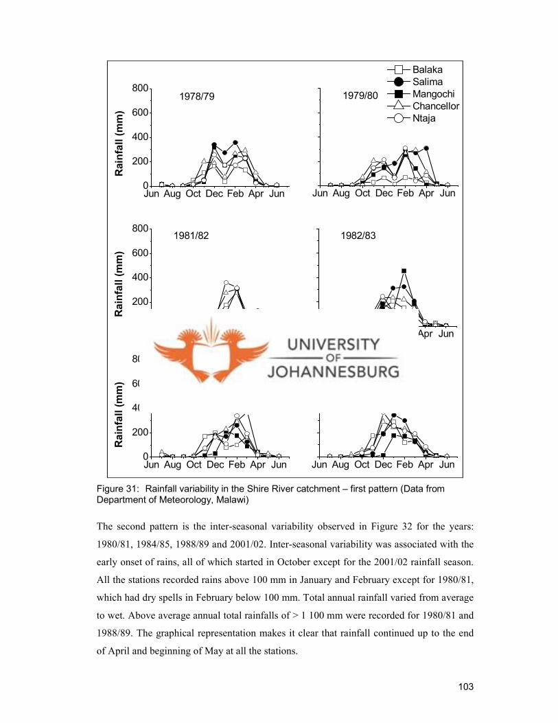
103
Jun Aug Oct Dec Feb Apr Jun0
200
400
600
800
Rainfall (mm)
1978/79
Jun Aug Oct Dec Feb Apr Jun
1979/80
Jun Aug Oct Dec Feb Apr Jun0
200
400
600
800
Rainfall (mm)
1981/82
Jun Aug Oct Dec Feb Apr Jun
1982/83
Jun Aug Oct Dec Feb Apr Jun0
200
400
600
800
Rainfall (mm)
1983/84
Jun Aug Oct Dec Feb Apr Jun
Balaka
Salima
Mangochi
Chancellor
Ntaja
1986/87
Figure 31: Rainfall variability in the Shire River catchment – first pattern (Data from Department of Meteorology, Malawi)
The second pattern is the inter-seasonal variability observed in Figure 32 for the years:
1980/81, 1984/85, 1988/89 and 2001/02. Inter-seasonal variability was associated with the
early onset of rains, all of which started in October except for the 2001/02 rainfall season.
All the stations recorded rains above 100 mm in January and February except for 1980/81,
which had dry spells in February below 100 mm. Total annual rainfall varied from average
to wet. Above average annual total rainfalls of > 1 100 mm were recorded for 1980/81 and
1988/89. The graphical representation makes it clear that rainfall continued up to the end
of April and beginning of May at all the stations.

104
Jun Aug Oct Dec Feb Apr Jun0
200
400
600
800
Balaka
Mangochi
Chancellor
Salima
Ntaja
Rainfall (mm)
Rainfall (mm)
1980/81
Jun Aug Oct Dec Feb Apr Jun
1984/85
Jun Aug Oct Dec Feb Apr Jun0
200
400
600
8001988/89
Jun Aug Oct Dec Feb Apr Jun
2001/02
Figure 32: Rainfall variability in the Shire River catchment – second pattern (Data from the Department of Meteorology, Malawi)
The third pattern is observed in Figure 33 for the years 1977/78, 1985/86 and 1987/88,
when the onset of rain was delayed until the second dekad of November at all stations
except Balaka, which experienced rain in October. Overall, all the stations recorded annual
rainfall above 800 mm a-1
, except Mangochi which had low rainfall (550 mm) in the
1985/86 rainfall season. High rainfall is observed in December and January, totalling a
mean monthly rainfall of < 300 mm. The rainfall season has demonstrated significant inter-
decadal variability associated with slightly low means in February (mean of 135 mm) and
above normal rains in March, with a mean of 348 mm.

105
Jun Aug Oct Dec Feb Apr Jun0
200
400
600
800Rainfall (mm)
1977/78
Jun Aug Oct Dec Feb Apr Jun
1985/86
Jun Aug Oct Dec Feb Apr Jun0
200
400
600
800
Balaka
Salima
Mangochi
Chancellor
Ntaja
Rainfall (mm)
1987/88
Figure 33: Rainfall variability in the Shire River catchment – third pattern (Data from the Department of Meteorology, Malawi)
Due to variability in the distribution and occurrence of rainfall, there are also possible
changes in the availability of water for plant growth, the regeneration of vegetation, river
flow and ground water recharge. Natural vegetation is highly sensitive to high or low
rainfall, which may in turn modify soil moisture and albedo.
The AVSWATX programme requires a set of rain gauges with representative distribution
over the catchment and daily values for precipitation quantities. It should be noted that
only five rainfall stations (Mangochi, Ntaja, Balaka, Salima and Chancellor College) were
used in this study. Although they are distributed across the catchment, the number is
smaller than would be ideal. The stations used met two basic criteria: location within the
study area (at representative points along the length of the catchment) and the existence of
sufficiently long observed records falling within the study period (1989-2002).
Nevertheless, the rainfall stations were considered to represent the main run-off
contributing sub-basins. The available meteorological stations are shown in Figure 34 and
the period of records within and surrounding the study area are shown in Table 23.

106
Salima
Chancellor College
Balaka
Mangochi
Ntaja
Liwonde
Salima
Chancellor College
Balaka
Mangochi
Ntaja
Liwonde
Figure 34: Weather stations and river gauging stations in the Shire River catchment
Table 23: Weather stations and available data
Station Altitude (m)
Rainfall Temp Relative Humidity
Windspeed Solar
radiation
Mangochi 480 1961 - 2006 1961 - 2004 1980 - 2000 1979 - 2003 1979 - 2003
Salima 520 1954 - 2006 1961 - 2005 no data no data no data
Balaka 660 1976 - 2006 1976 - 2006 no data no data no data
Ntaja 670 1971 - 2006 1985 - 2004 no data no data no data
Chancellor College
650 1975 - 2006 1982 - 2006 no data 1975 - 2000 no data
River discharge
Daily stage readings of the Shire River at two stations were obtained from the Hydrology
Department of the Ministry of Water Resources of Malawi (Table 24). There are only two
flow-gauging stations on the Shire River within the study area, one at the inlet to the valley

107
at Mangochi (1T1), and one at Liwonde (1B1), taken as the outlet (Figure 34). There are
no gauging stations anywhere on the tributaries within the catchment.
The streamflow at Mangochi includes the flow from the catchment and the main outflow
from Lake Malawi. This complicates the calculation of the net catchment flow from the
Liwonde catchment (the area being modelled), as the main streamflow is an order of
magnitude larger than the catchment generated flow. How these flows were processed to
derive the net catchment flow for Liwonde is described below.
Table 24: Daily river flow data
Station Area (km2) Period
Mangochi 12 650 1975 – 2001
Liwonde 13 020 1948 – 2002
The raw data as received from the Hydrology Department of the Ministry of Water
Resources in Malawi required critical analysis to check the reliability and quality of the
data. Figure 35 shows a time-series plot of inflow and outflow stream data recorded from
1976 to 2000 for the Shire River catchment as received.

108
Figure 35: Time series streamflow for the Shire River Mangochi (inflow) and Liwonde (outflow) for the period 1976 - 1981: data as received
There are regular data records for the period from 1976 to 1981, except for three days in
1978 for which there were no recorded values. The consistency and few data gaps in the
time series makes this period eligible for analysis.
The period between 1982 and 1983 depicts dry years in terms of rainfall, while from 1984
to 1988 the rains were within the normal average. There are, however, major
inconsistencies between inflow and outflow – outflows were much lower than inflows
from 1982 to 1983. The discrepancy between inflow and outflow is too large to be
attributed to any possible loss, extraction or consumption between the inflow and outflow
weirs. Although rainfall in the catchment was lower than the long-term average during
1982 and 1983, the reduction is not sufficient to explain the discrepancy. In the absence of
a natural physical cause, the discrepancies could be attributed to gauge malfunctioning or
errors in recording. Data from these years are unusable for this investigation.
The data recorded from 1984 to 1986 are consistently accurate, except for two days in
1984 where there are data gaps and outliers. Data from this period was usable for this
study.

109
Data records from 1987 to 1988 comprise a complete data set. However, imbalances
between inflow and outflow were questionable, with inflow much higher than the outflow.
These could be due to recording errors at the outlet gauging station, as rainfall seems to be
high during this period. Rainfall contributes to higher flows during the wet season, which
is not demonstrated in this case. Thus, these data could not be utilised for this study.
From 1992 to 2000, data collection appeared to be inconsistent, with numerous data gaps
in the time series, specifically for the outflow monitoring station. The outflow is uniform
with season, instead of showing the expected major seasonal variations of prior years. The
data set for this period was thus regarded as unreliable and of no use for this study.
Based on the above evaluation, usable subsets were selected from the Shire River
streamflow data, between 1977 and 1981 for calibration of the hydrological model and for
the land cover change application (Figure 36) and between 1984 and 1985, for validation
of the hydrological model. Data cleaning was done by interpolation for days for which data
were missing or misrepresented by unphysical spikes or drops.
0
200
400
600
800
1000
1200
Jan-77
May-77
Sep-77
Jan-78
May-78
Sep-78
Jan-79
May-79
Sep-79
Jan-80
May-80
Sep-80
Jan-81
May-81
Sep-81
Inflow outflow
Streamflow (m3 s-1)
0
200
400
600
800
1000
1200
Jan-77
May-77
Sep-77
Jan-78
May-78
Sep-78
Jan-79
May-79
Sep-79
Jan-80
May-80
Sep-80
Jan-81
May-81
Sep-81
Inflow outflow
Streamflow (m3 s-1)
Figure 36: Streamflow data for 1977 - 1981, data as received

110
The inflow and outflow for 1977 - 1981 shows a consistent trend except for a few days
where there are data gaps and outliers. There are also imbalances between the inflow and
outflow, which could be the result of several factors. The main water balance components
such as precipitation, evaporation, interflow and baseflow could explain some of the flow
imbalances between inflow and outflow. Lake Malombe, a large shallow lake, might
provide hydraulic resistance to streamflow inducing delays, especially during the dry
season when flows are generally low. In addition, this variation may also be caused by
unknown data-recording errors in both inflows and outflows, as data were recorded
manually. For example, from 13 to 18 July 1977 there was a drop in stream outflow by
more than 50 m3 s
-1 – probably due to instrument malfunctioning, as there is no plausible
natural explanation for this drop. Between 17 October and 6 November 1978, the outflow
data records were consistently below 220 m3 s
-1, while no inflow data were recorded from
1 to 6 November 1978. These inconsistencies could be due to instrument malfunctioning or
maintenance.
Another questionable period is the record from 13 to 18 May 1979, where three
consecutive days with identical values, followed by two days with the identical, but lower
readings, during a period of generally increasing streamflow, where recorded. The values
from 11 to 14 March 1980 are also questionable, as the inflow was consistently 800m3
s-1
.
There is also uncertainty in data recorded from 19 to 25 March 1980. In this case the
inflow was uniform over 6 days at 813 m3
s-1
, an improbable result suggesting that a value
had been copied to account for missing readings. Another human error recording probably
occurred on 26 July 1980: here the reading shows a singular high value of 932 m3
s-1
– a
non-physical jump of ~100 m3
s-1
, taking into account the previous day and the following
day records. A corrected value of 832 m3
s-1
was inserted in place of 932 m3
s-1
, assuming
that a recording error of a single digit had occurred. There is also uncertainty in the data
measurements from 16 to 30 April 1981, where all the inflow recorded were above
1 030 m3
s-1
, having increased suddenly from 940 m3 s
-1. Such distorted data sets could be
due to errors in recording or malfunctioning of the gauging instrument.
The identified misrepresented data constitutes 3.8% of the entire period (1977 to 1981).
The correction and interpolation of ~4% is considered small enough that these corrections
do not fundamentally alter the integrity of the streamflow records. After data cleaning by
the deletion of questionable records and interpolation, the calibration and validation results

111
presented are the best achievable. Data was cleaned further based on a weighted five-point
smoothing routine, using the mean and standard deviation. Figure 37 shows the smoothed
outflow data for the Shire River. This smoothing is justified by the fact that the time
constants of the response of a large catchment such as the Shire River catchment, is longer
than the one day measurement frequency at the gauging stations.
Hydrological characterisation of Shire River catchment based on hydrological variables
Following data smoothing, a hydrological characterisation was conducted to identify
contributing water sources and to understand the flow processes of the Shire River,
including specifically the interplay between inflows from Lake Malawi, buffer storage and
flow retardation within Lake Malombe, and normal catchment processes. The
characterisation analysis was carried out for five-year period between January 1977 and
December 1981. A number of approaches have been used to characterise the
ground/surface water interaction and the role it plays in streamflow of the Shire River. The
approaches include correlation/qualitative analysis of streamflow and precipitation.
0
200
400
600
800
1000
1200
Jan-77
May-77
Sep-77
Jan-78
May-78
Sep-78
Jan-79
May-79
Sep-79
Jan-80
May-80
Sep-80
Jan-81
May-81
Sep-81
Outflow (m3 s-1) Inflow (m3 s-1)
Stream flow (m3 s-1)
0
200
400
600
800
1000
1200
Jan-77
May-77
Sep-77
Jan-78
May-78
Sep-78
Jan-79
May-79
Sep-79
Jan-80
May-80
Sep-80
Jan-81
May-81
Sep-81
Outflow (m3 s-1) Inflow (m3 s-1)
Stream flow (m3 s-1)
Figure 37: Smoothed daily streamflow data from 1977 - 1981
The quantitative approach entailed correlations between (i) flow at the exit from Lake
Malawi into the Shire River at Mangochi gauging station (1T1), and (ii) flow discharges at
the outlet of the Shire catchment observed at Liwonde gauging station (1B1). Based on the
result obtained from the correlation between inflow and outflow characterisation, an

112
automated baseflow separation technique based on master recession curves, developed by
Arnold et al., [1995], was used to separate the observed stream outflow components into
baseflow and surface flow. This technique was developed and successfully used by Arnold
and Allen [1999] for estimating baseflow and annual ground water recharge from
streamflow hydrographs. Baseflow values obtained after the filter represent flow from
Lake Malawi, while surface flow comprises flow from the catchment (hereafter referred to
as catchment streamflow). Furthermore, a quantitative analysis was conducted between
precipitation data for gauging stations located within the catchment and catchment
streamflow.
Since the focus of this study was to evaluate the effects of derived quantitative land cover
changes on hydrological processes, the catchment streamflow, obtained from the above
inflow/outflow characterisation, was used for AVSWATX calibration and model
application. The catchment streamflow time series resulting from the above processing is
depicted in Figure 38. This data set is used for further modelling and evaluation of land
cover - hydrological interactions.
0
25
50
75
100
Jan-77
May-77
Sep-77
Jan-78
May-78
Sep-78
Jan-79
May-79
Sep-79
Jan-80
May-80
Sep-80
Jan-81
May-81
Sep-81
Catchment streamflow (m3s-1)
Catchment stream outflow (m3 s-1)
0
25
50
75
100
Jan-77
May-77
Sep-77
Jan-78
May-78
Sep-78
Jan-79
May-79
Sep-79
Jan-80
May-80
Sep-80
Jan-81
May-81
Sep-81
Catchment streamflow (m3s-1)
Catchment stream outflow (m3 s-1)
Figure 38: Smoothed catchment streamflow data, 1977 - 1981

113
Sensitivity analysis and auto-calibration
Sensitivity analysis is an instrument for the assessment of input parameters in relation to
their impact on model performance [Lenhart et al., 2002]. Model sensitivity is defined as
the change in model output per unit change to an input parameter. Sensitivity analysis may
be used to evaluate how model outputs vary over a range for a given input variable. Some
researchers have noted that sensitivity analysis and calibration are difficult with a large
number of parameters [Ndomba, 2007]. In general, parameter sensitivity analysis aids the
user in reducing the number of parameters that must be varied by identifying the critical
parameters and allowing insensitive parameters to be held fixed, thereby reducing the
complexity and computational time required for model calibration.
The theoretical background of the sensitivity analysis method that is implemented in SWAT
is called the Latin Hypercube One-Factor-At-a-Time (LH-OAT) design and was proposed
by Morris [1991]. The LH-OAT sensitivity analysis combines the strength of global and
local sensitivity methods of analysis. Prior to the calibration and validation process, a
sensitivity analysis based on the integration of LH-OAT was performed to reduce
uncertainty and provide parameter estimation guidance. There are more than sixty
parameters in the AVSWATX model. Some of these parameters vary by sub-basin, land
cover and soil type. This variation may increase the number of parameters substantially.
However, a good number of other parameters are empirical or AVSWATX-specific. For
example, AVSWATX uses the SCS curve number method to estimate surface Curve
Number [USDA-SCS, 1972]. In the present study, twenty-seven parameters were included
in the analysis. The parameters selected have the greatest sensitivity to the hydrology of
the system and are related to land cover, run-off, groundwater penetration and soil
characteristics [Van Griensven, 2002].
Sensitivity analysis was performed for each sub-basin of the Shire River basin to reduce
uncertainty and provide parameter estimation guidance for the calibration steps. The
sensitivity analysis was carried out for a period of five years, including the calibration
period from 1977 to 1981. Parameter values as recommended by Van Griensven [2002]
were used as initial values for the analysis. Other researchers in the region, such as
Ndomba [2007], have successfully applied this approach.
During the sensitivity analysis, AVSWATX estimates the relative sensitivity (RS) of various
parameters. Since the parameters are of different types and vary in different magnitudes,

114
this assists in comparing the effects that different parameters have on the parameter
estimation process. Lenhart et al. [2002] categorized the relative sensitivity into four
classes. According to this classification, RS values between 0 - 0.05 are categorised as
small, while RS values between 0.05 - 0.2 are categorised as medium. On the higher side,
RS values greater than 0.2 - 1.0 and greater than one are classified as high or very high,
respectively. The relative sensitivity values found in the parameter estimation process were
categorized into these four classes. Sensitivity evaluations were carried out, producing nine
parameters for modelling. Identified parameters and relative sensitivities are presented in
Section 4.3.
Following the sensitivity analysis, auto-calibration was done for sensitive parameters only
to obtain the optimum values. The watershed model AVSWATX includes an option to
perform automatic calibration using the optimization algorithm. The automatic calibration
procedure in AVSWATX is based on the Shuffled Complex Evolution algorithm developed
at the University of Arizona (SCE-UA). SCE-UA is a global search algorithm that
minimizes a single objective function for up to 16 model parameters [Duan et al., 1992].
SCE-UA has been widely used in watershed model calibration and other areas of
hydrology such as soil erosion, sub-surface hydrology, remote sensing and land-surface
modelling. It has been found to be robust, effective and efficient. The SCE-UA has also
been applied with success to AVSWATX for hydrologic parameters [Eckhardt and Arnold,
2001] and hydrologic and water quality parameters [Van Griensven, 2002].
The auto-calibration tool, based on the SCE_UA algorithm available in AVSWATX, was
used to calibrate eight parameters in the model that govern streamflow in Shire River
catchment. The auto-calibration provides three methods of updating the parameters: (i)
replacement by a new value, (ii) adding fractionally to an initial value, and (iii) multiplying
an initial value by a factor. The second and third methods are references relative to an
initial value. This allows a lumped calibration of distributed parameters, which ensures that
the relative physical meaning is maintained (for example, the CN of forest is lower than the
CN of subsistence agriculture).
4.2.2 Model setup
The hydrological modelling using SWAT was based on the application of the Graphical
User Interface (GUI) of AVSWATX, which is embedded in ArcView [Di Luzio et al., 2001].
Tools are accessed through pull-down menus that are introduced in the various ArcView

115
GUI and custom dialogues. AVSWATX processes mapped land cover and soils data as well
as a Digital Elevation Model (DEM) to create a set of default model input files. Within
each sub-basin, Hydrological Response Units (HRUs) are created by AVSWATX. HRU
creation in AVSWATX requires land cover and soil threshold inputs [Di Luzio et al., 2001]
to define the level of spatial detail provided by the model. These thresholds are applied to
each sub-basin and function to control the size and number of HRUs created. Various GIS
data pre-processor modules were developed in the course of modelling the catchment
including catchment delineation, input map characterization and processing, stream and
outlet definition, the computation of geomorphic parameters and characterization of the
land cover and soil. Interactions between surface flow and subsurface flow in AVSWATX
are based on a linked surface to sub-surface flow model developed by Arnold et al. [1994].
The input data were prepared to the required format for input to the AVSWATX model. The
processing of spatially distributed data is achieved in a four-step approach.
The first step of the modelling process using AVSWATX is the catchment delineation,
which uses the DEM. Stream-catchment delineation identified the flow elements and
contributing areas (sub-basins) of the upper Shire River hydrological system. From the
DEM, a stream map was created using a minimum contributing source area (CSA)
threshold value of 8% to define lengths and numbers of stream channels. The threshold
value for the map represents the number of cells in the DEM that receives run-off from a
certain number of cells. All cells receiving run-off are classified as streams. Figure 39 is a
schematic representation of a grid-based catchment delineation showing flow from a DEM.
The stream map is used to locate outlet regions for individual sub-basins.
In the second step, the catchment is divided into model elements according to the land
cover properties of the area. This step requires a land cover classification system with
appropriate attribute data to be accepted by the program. The land cover layer generated in
this study using the FAO Land Cover Classification System (LCCS) classification (see
Chapter 2) was used. The LCCS classification system is not among the default schemes in
the AVSWATX program, but there is an option for user-defined land cover. This requires a
translation to be made in certain codes [Neitsch et al., 2005]. AVSWATX connects these codes
(Table 20) with the land cover/plant growth database through a look-up table.

116
Grid lines
Cell
Catchment outlet
Flow channel
Grid lines
Cell
Catchment outlet
Flow channel
Figure 39: Grid based discretisation and concept of flow path used in a cell
In the third step, the catchment is divided into model elements using a soil layer containing
soil properties of the catchment. All soil parameters are linked through look-up tables.
AVSWATX uses soil hydrological groups to define soil hydraulic properties. The drainage
of the soils is described according to the FAO classes [FAO/UNESCO, 2003] and used to
assign hydrological groups (in run-off generation perspective) based on permeability and
infiltration characteristics. The importance of assigning soil hydrological groups is that
they are used in AVSWATX to assign curve numbers (CN) for the land cover and soil
combinations, also known as HRUs, which are used in the equations to calculate the
partition between surface run-off and soil infiltration.
The catchment created in Step 1 is then intersected with land cover and soil data, and
parameters necessary for the hydrological model runs are estimated through a series of
look-up tables. This discretisation resulted in the definition of 13 sub-basins (Figure 40). In
AVSWATX, a catchment is delineated into sub-basins, which are then further subdivided
into HRUs. HRUs consist of homogeneous land cover and soil types. Based on two options
in AVSWATX, HRUs may represent either one sub-basin area with a dominant land cover
or soil type, or several homogeneous HRUs representing unique combinations. In this

117
study, sub-basin areas with a dominant land cover or soil type were used for the
simulations for computational efficiency. Each sub-basin delineated within AVSWATX is
simulated as a homogeneous area before estimates are summed for the basin.
The fourth stage is the incorporation of meteorological data. AVSWATX requires daily
meteorological data that either can be read from a measured data set or can be generated by
a weather generator model. In this study, a statistical weather generator file WXGEN
[Sharpley and Williams, 1990] was prepared to generate climatic data and fill in gaps in
the missing records from climatic data obtained. The weather generator was also used to
simulate daily values for variables from aggregated monthly solar radiation, as these were
only available as monthly values.
Figure 40: Sub-basins for the Shire River catchment
In to the case of precipitation, data can be put into the model from available measured
values. The distribution of precipitation measuring stations is not uniform across the
catchment, but is consistent enough, compared to the data availability in the country
overall. Most of the raw data vectors are incomplete to greater or lesser extents. However,
they are left as they are because AVSWATX uses a model developed by Nicks [1974] to
generate daily precipitation for simulations to interpolate missing data in the measured

118
records. This program fills data gaps or extends time series of daily data based on monthly
statistics. The monthly statistics, however, are based on long series of daily data. The
precipitation generator uses a first-order Markov chain model. Thus, input to the model
uses the monthly values for precipitation and the number of wet days per month. Given the
wet-dry state, the model determines stochastically whether precipitation occurs to obtain
the required daily inputs.
When a precipitation event occurs, the amount is determined by generating from a skewed
normal daily precipitation distribution or a modified exponential distribution. In this study,
a skewed normal daily precipitation distribution was opted for. Precipitation data were
retrieved by the AVSWATX input interface for the weather station nearest the centre of the
sub-basin. The details of the weather generator parameters and equations are given in the
SWAT model documentation [Neitsch et al., 2005].
4.2.3 Modelling the Shire River catchment
Calibration parameters
Simulation of the rainfall run-off model was based on previous experience and modelling
techniques published by various researchers [Ndomba, 2007; Ndomba et al., 2005; Van
Liew et al., 2005]. These techniques include a curve number method for calculating the
surface run-off [USDA-SCS, 1972], a first order Markov Chain Skewed Normal to
determine rainfall distribution, the Penman-Monteith method to compute potential
evapotranspiration, and the Muskingum routing method for flow routing water through
channel networks. Calibration was based on distributed unfilled rainfall data, whereby the
model uses a built-in weather generator to interpolate missing rainfall values.
The objective of a calibration procedure is to estimate the values for parameters that cannot
be assessed directly from field data. Parameter estimation is designed to reduce the
uncertainty of the modelling process. A typical approach is to select an initial estimate for
the parameters from within previously specified ranges. The parameter values are then
adjusted to optimise the agreement between model behaviour and that of the watershed.
The process of adjustment can be done manually or by computer-based automatic methods.
According to Refsgaard and Storm [1996], three types of calibration procedures can be
differentiated: trial-and-error manual parameter adjustment, automatic numerical parameter
optimization and a combination thereof. For hydrological model calibration, a combination
119
of manual and automatic procedures has been recommended [Gan, 1988]. Manual
calibration alone is tedious, time consuming, and requires an experienced researcher to
anticipate optimum parameter combinations. Thus, there have been several efforts towards
development of automated calibration methods. Automatic calibration, however, relies
heavily on the optimisation algorithm and the specified objective function. If not carefully
specified, the process might lead to a local optimisation point in the multidimensional
space that is unphysical or poorly matched to the overall catchment behaviour. Therefore,
in the calibration process for this study, a combination of manual and automatic parameter
estimation was adopted to optimise the nine selected parameters.
Available catchment streamflow data from January 1977 to December 1981 (5 years) were
used for model calibration, while data from January 1984 to December 1985 (2 years) were
used for model validation. Calibration was done at daily time intervals by comparing
modelled and measured streamflows at the outlet point of the catchment at the Liwonde
gauging station. Parameters through AVSWATX interface were changed in a semi-
distributed way (i.e. sub-basinwise). The optimisation was conducted on one or two
parameter(s) at a time depending on the computation resource required for a particular
simulation. The parameter ranges were selected with reference to relevant literature and
guidance from an experienced modeller (P.M. Ndomba, private communication).
Validation
To use any predictive watershed model for estimating the effectiveness of potential land
cover changes, the model must be first calibrated against measurements, and then be
validated (without further parameter adjustment) against an independent set of measured
data. This testing of a model on an independent data set is commonly referred to as model
validation. Model calibration determines the best or at least a reasonable, parameter set,
while validation ensures that the calibrated parameters set performs reasonably well under
an independent data set. Provided the model’s predictive capability is demonstrated as
reasonable in the calibration and validation phase, the model can be used with confidence
for future predictions in different land cover and management scenarios.
In this study, calibration and validation procedures presented in the SWAT user manual
were followed [Neitsch et al., 2005]. Calibration for water balance and streamflow was
done first for average annual conditions. Once the run was calibrated for annual conditions,
we shifted to the monthly records to fine-tune the calibration. Model efficiency expresses
120
the fraction of the measured streamflow variance that is reproduced by the model. Model
outputs were calibrated to fall within the average measured values and then model
performance statistics (ENS) (Equation 18) were evaluated by comparing simulated and
measured annual, monthly and daily catchment streamflows. Calibration and validation
were performed for the selected periods. The objective functions used to test the model
performance were Nash and Sutcliffe simulation efficiency (ENS) and the Index of
Volumetric Fit (IVF):
( ) ( )[ ]∑ ∑ −−−= 22/1 meanobssimobsNS QQQQE (18)
where ENS is coefficient of simulation efficiency, Qobs is the measured streamflow in each
model step (m3 s
-1) (in this case annual, monthly and daily), Qsim is the simulated
streamflow in each model step (m3 s
-1) (in this case annual, monthly and daily) and Qmean is
the mean measured streamflow in each model step during the evaluation period (m3 s
-1) (in
this case annual, monthly and daily).
Simulation results are good for values for values of ENS ≥ 0.75, while for values of ENS
between 0.75 and 0.36, the simulation results are acceptable. ENS values less than 0.36 are
unacceptable [Popov, 1979]. These values were considered adequate statistical values for
acceptable calibration for the purposes of this study. In addition to quantitative model
performance evaluation, simulated and measured flows were compared in graphical
displays to convey qualitative information such as trends and distribution patterns of flows.
4.2.4 Testing effects of land cover change
To test the assumption that land cover change has affected watershed streamflow, further
simulations were performed using the land cover classifications derived from two different
Landsat images in 1989 and 2002 respectively for the same rainfall regime: the 1977 to
1981 period. The 1989 land cover map was used for the calibration and validation runs of
the model. To isolate and evaluate the variability of streamflow due only to land cover
changes, the AVSWATX model was re-run using the 2002 land cover map, while all the
other input variables remained constant.
4.2.5 Scenario generation
Scenario analysis is a process of evaluating possible future events by considering
alternative possible outcomes. This analysis is designed to facilitate decision-making and
assessment through a complete consideration of possible outcomes and their implications.

121
The development of strategies for water resource planning and management and the
assessment of impacts of potential environmental change are often guided by the analysis
of multiple future scenarios.
The sensitivity the Shire River catchment hydrological system to future land cover changes
were analysed using AVSWATX model, by formulating a range of land cover change
scenarios. As a first test, two extreme limiting scenarios were considered – total
deforestation and total forestation. The modelling process was carried out to assess
influences on run-off components and total water yield in response to these bounding
conditions. Most likely changes to land covers are conversion from rangeland and forest to
agriculture in a land-degradation (pessimistic) scenario, and conversion from agricultural
land to rangeland and forest in a land-conservation (optimistic) scenario. Changes to all
three of these land cover types have influences on catchment hydrology. Urbanisation
equally affects hydrological processes. However, it was excluded from scenario analysis,
as it constitutes a small fraction of the total area, and in Malawi, still a small area of
change. For the second stage scenario modelling, a range of scenarios were considered, in
which fractional changes were made to these three land cover classes for the pessimistic
and optimistic trends. These sensitivity analyses were aimed at providing insights on the
proper behaviour of the model, and at generating plausible scenarios for guiding land use
policy and development strategies.
Each scenario was created by changing patches of selected land cover type one into target
land cover type two. Land cover classifications derived from the 2002 Landsat image were
used as the baseline. The type two land covers were defined by assigning changed areas to
the baseline classification, selected randomly by computer simulation within the selected
land cover type, and spread evenly over the target catchment. The total area affected in
each scenario was an assigned proportion of the original area of land cover type one.
Scenarios were developed for changes in the original areas of rangeland and forestry in
increments of 10%, 20%, and 40%. Scenario runs were conducted for these incremental
steps separately for each of the two types of land cover, for degradation and conservation
scenarios. Combined scenarios were run for the conservation scenario only, in which
agricultural land reverts to rangeland and forest, each changed by the medium and
maximum increments (20% and 40%) to evaluate combined effects on the hydrology.

122
A narrative description of the scenarios is provided below.
Business as usual
For the business as usual baseline scenario, the 2002 land cover grid (Chapter 2) was used.
Compared to the 1989 land cover map, the following gross changes are noted in the 2002
land cover map: Forests are reduced in the lower and upper escarpments within the
catchment in favour of transitional woodland-shrub; there is transformation of savanna
shrubland areas into cultivated and grazing land; and there are major increases in
grassland areas. The hydrological model was run with the 2002 land cover grid
unchanged, and the 1989 climatic data set. (Note that the streamflow data for 2002 was
unusable. Therefore, it was not possible to carry out a full validation of the AVSWATX
model using 2002 climatic records and the 2002 land cover classification. The AVSWATX
model, validated using the 1989 land cover image and earlier catchment streamflow, was
used instead.)
Land degradation scenario
The second scenario, termed land degradation, represents an unfavourable scenario,
including accelerated land cover change with extensive deforestation. In this case,
significant fractions of forest and savanna shrubland areas are transformed into the
category agricultural land generic, which includes subsistence agricultural areas,
transitional woodlands and sparsely vegetated areas. There is a significant decrease in the
area of the woodlands because of the increased use of land for agriculture to produce food
for the growing population. Although this scenario may imply increasing built-up areas, as
a fraction of the catchment this change is minor and so the size of the built-up area remains
constant. Three different extents of deforestation of forest deciduous and of rangeland
brush respectively were tested as shown in Table 25, indicating a range of increasingly
pessimistic scenarios up to 2020.

123
Table 25: Characteristics of 2002 land cover data and deforestation scenarios
Scenario Base line 1 2 3 4 5 6
Land use/Land cover Business as usual
Rangeland brush converted to Agricultural land generic
Forest deciduous converted to Agricultural land generic
Descrip-tion
Land cover 2002
10% 20% 40% 10% 20% 40%
Area (ha) 200 570 211 620 222 669 274 816 208 082 215 594 230 618 Agricultural land generic % 40.9 43.2 45.4 56.1 42.5 44 47.2
Area (ha) 110 495 99 445 88 396 66 297 110 495 110 495 110 495 Rangeland brush % 22.6 20.3 18.1 13.6 22.6 22.6 22.6
Area (ha) 75 119 75 119 75 119 45 071 67 607 60 095 45 071 Forest deciduous % 15.3 15.3 15.3 15.3 13.8 12.3 9.1
Land categories not changed in scenario analysis
Area (ha) 37 100 37 100 37 100 37 100 37 100 37 100 37 100 Water
% 7.6 7.6 7.6 7.6 7.6 7.6 7.6
Area (ha) 5 775 5 775 5 775 5 775 5 775 5 775 5 775 Residential medium density % 1.2 1.2 1.2 1.2 1.2 1.2 1.2
Area (ha) 24 412 24 412 24 412 24 412 24 412 24 412 24 412 Wetland
% 4.9 4.9 4.9 4.9 4.9 4.9 4.9
Area (ha) 36 629 36 629 36 629 36 629 36 629 36 629 36 629 Forest mixed % 7.5 7.5 7.5 7.5 7.5 7.5 7.5
Land conservation
The third scenario, termed land conservation, represents of the creation of a greener
environment through management and re-forestation. This scenario involves the
conversion of potentially vulnerable areas (subsistence agricultural land) into forest and
savanna woodlands. Different extents of forestation were investigated, as shown in Table
26, indicating an optimal scenario up to 2020.

124
Table 26: Characteristics of simulated land cover forestation scenarios
Scenario Base line
7 8 9 10 11 12
Busi-ness as usual
Savanna converted to Agri-
land
Agricultural land converted to Forest
Deciduous
Agri-land to both Savanna and Forest
Land use/Land cover
Descrip-tion
Land cover 2002
20% 40% 20% 40% 20% 40%
Area (ha) 200 570 160 456 120 342 160 456 120 342 120 40 114 Agricultural Land Generic % 40.9 32.7 24.6 32.7 24.6 24.6 8.2
Area (ha) 110 495 150 609 190 723 110 495 110 495 150 609
190 723 Rangeland brush % 22.6 30.7 38.9 22.6 22.6 30.7 38.9
Area (ha) 75 119 75 119 75 119 115 233 155 347 115 233
155 347 Forest Deciduous % 15.3 15.3 15.3 23.5 31.7 23.5 31.7
Land categories not changed in scenario analysis
Area (ha) 37 100 37 100 37 100 37 100 37 100 37 37 100 Water
% 7.6 7.6 7.6 7.6 7.6 7.6 7.6
Area (ha) 5 775 5 775 5 775 5 775 5 775 5 775
5 775 Residential medium density % 1.2 1.2 1.2 1.2 1.2 1.2 1.2
Area (ha) 24 412 24 412 24 412 24 412 24 412 24 412
24 412 Wetland
% 4.9 4.9 4.9 4.9 4.9 4.9 4.9
Area (ha) 36 629 36 629 36 629 36 629 36 629 36 629
36 629 Forest mixed
% 7.5 7.5 7.5 7.5 7.5 7.5 7.5
Absolute and relative changes in annual values of surface flow, baseflow and total water
yield were calculated for each scenario. Average annual and monthly outflows simulated at
the catchment outlet for the various change scenarios were then compared to the baseline
case.
4.3 Results and discussion
4.3.1 Hydrological characterization of Shire River catchment using hydrological
variables
Characterisation analysis in the upper Shire River has found that there is a strong positive
correlation (r2 = 98%) between measured river outflow from Lake Malawi measured at
Mangochi (Gauge No. 1T1) and the Shire River measured outflow, measured at Liwonde
(Gauge No. 1B1). This indicates that the inflow from Lake Malawi flowing into the Shire
River flows out from the river system at Liwonde, with minimal perturbation from the
Shire River catchment.
Although the statistical analysis suggests that the main source of inflow to Shire River is
Lake Malawi, a quantitative analysis suggests possible contributions from the catchment.

125
The hydrological variables used included daily rainfall and daily catchment streamflow
measured at the outlet (Liwonde). The results of the qualitative analysis showed that there
is an association between streamflow and the onset and offset of rainfall patterns,
suggesting that catchment rainfall does account for a substantial amount of groundwater
flow and surface flow into the river. As shown in Figure 41 at the onset of the rainy season
there is a steady increase in streamflow recorded at the outlet, while during the dry season
decreased flows have been recorded. At the onset of the rains, water losses by plant uptake
and evaporation decline because of milder temperatures. Natural streamflow increases as
rains produce more run-off. During the dry months of late April to late October,
evaporation and water used by plants decrease run-off and the amount of groundwater
available to support streamflow. Hence, streamflow declines. Precipitation is the most
significant climate variable affecting daily streamflow gains.
0
40
80
120
160
200
Jan-77
May-77
Sep-77
Jan-78
May-78
Sep-78
Jan-79
May-79
Sep-79
Jan-80
May-80
Sep-80
Jan-81
May-81
Sep-81
0
40
80
120
160
200
Catchment streamflow (m3 s-1) Rainfall (mm)
Catchment streamflow (m3 s-1)
Rainfall (mm)
0
40
80
120
160
200
Jan-77
May-77
Sep-77
Jan-78
May-78
Sep-78
Jan-79
May-79
Sep-79
Jan-80
May-80
Sep-80
Jan-81
May-81
Sep-81
0
40
80
120
160
200
Catchment streamflow (m3 s-1) Rainfall (mm)
Catchment streamflow (m3 s-1)
Rainfall (mm)
Figure 41: Time series plots of catchment streamflow and rainfall
The characterisation results indicate contributions to the Shire River flow from both Lake
Malawi and the Shire River catchment. However, to analyse the effects of catchment land
cover changes on surface run-off and seasonal river variations, water from Lake Malawi
flowing through the river system was excluded from the modelling process. The study only
modelled the catchment streamflow, which comprises surface run-off and baseflow from
the catchment.

126
4.3.2 Modelling of the Shire River catchment
Sensitivity analysis
For the Shire River catchment, sensitivity analyses showed that from the total of 28
parameters, only fourteen parameters revealed significant effects on the flow simulation.
Sensitivity analysis results are shown in Table 27, classified in terms of relative sensitivity,
as defined by Lenhart et al. [2002].
Table 27: Relative sensitivity values of the optimised parameters
Parameter Relative
sensitivity RS Category Ranking
SCS run-off curve number, CN2 3.820 very high 1
Soil evaporation compensation factor, ESCO 0.277 high 2
Soil available water capacity (mm WATER/mm soil), SOL_AWC
0.167 medium
3
Soil depth (mm), SOL_Z 0.053 medium 4
Maximum canopy storage (mm), CANMX 0.044 small 5
Saturated hydraulic conductivity (mm h-1), SOL_K 0.040 small 6
Surface run-off lag time (days), SURLAG 0.024 small 7
Average slope steepness (m/m), SLOPE 0.022 small 8
Baseflow alpha factor (days), ALPHA_BF 0.015 small 9
Moisture soil albedo, SOL_ALB 0.006 small 10
Channel effective hydraulic conductivity, CH_K2 0.006 small 11
Manning’s n value for main channel, CH_N 0.004 small 12
Average slope length, SLSUBBSN 0.003 small 13
Ground water “revap” coefficient, GW_REVAP 0.001 small 14
The sensitivity analysis identified the parameters SCS run-off curve number (CN2) and Soil
evaporation compensation factor (ESCO) as highly sensitive. Soil available water capacity
(SOL_AWC) and Soil depth (SOL_Z) were categorised as having medium sensitivity. The
rest of the parameters were found to have smaller relative sensitivities. It should be
mentioned that within the “small” relative sensitivity group, parameters that generally
govern the surface and sub-surface hydrological processes and have more physical
meaning to stream routing were selected for model optimisation. These parameters include
Surface run-off lag time (SURLAG), Saturated hydraulic conductivity (SOL_K), Baseflow
alpha factor (ALPHA_BF) and Ground water “revap” coefficient (GW_REVAP).
Five other low sensitivity parameters, not considered critical, were held fixed at default
values. These comprised Maximum canopy (CANMX), Average slope steepness (SLOPE),

127
Moisture soil albedo, (SOL_ALB), Channel effective hydraulic conductivity (CH_K2),
Manning’s n value for main channel (CH_N) and Average slope length (SLSUBBSN).
Auto-calibration
In the case of a new model application to an un-calibrated catchment, it is recommended
that the entire list of sensitive parameters be explored. Researchers working in well-
calibrated catchments have ended up using only a few of the most sensitive parameters
with confidence [Van Liew et al., 2005; Yapo et al., 1996]. However, for this study, the
eight sensitive parameters selected using the sensitivity analysis and based on physical
considerations, were optimised during calibration, following procedures incorporated in
the AVSWATX model.
Initial lower and upper default and final calibrated values are presented in Table 28. As
noted in the table, values for the SCS run-off curve number (CN2) and soil available water
capacity (SOL_AWC) are expressed as percentage change from the default value, and were
modified by multiplication of a relative change. High values of CN2, up to more than 80,
indicate greater contributions of precipitation to surface run-off than to subsurface flow.
The remaining parameters were calibrated by replacement of initial values.
Table 28: Parameter values calibrated in SWAT using the auto-calibration tool
Parameter Units Lower bound
Upper bound
Initial default value
Optimum value
Calibrated value
74 (RNGB) 7.4% 79
83 (AGRL) 4.2% 86
CN2*
-10 +10
73 (FRST) -7.5% 68
SOL_AWC* -50 +50 0.13 (688) 0.50% 0.07
mm WATER/mm
soil 0.10 (644) 0.90% 0.09
ESCO 0 1 0.950 0.90 0.900
Surlag days 0.5 10 4.0 0.70 0.70
GW_Revap 0.02 0.2 0.02 0.08 0.08
Alpha_BF days 0 1 1 0.007 0.007
Sol_z mm -50 50 300 300 300
Sol_k mm h-1 -50 50 38 38 38
CN2* and SOL_AWC* parameter values expressed as percent change from default values

128
Streamflow calibration, validation and model evaluation
Model simulation results are presented on an annual, monthly and daily basis for the
calibration and validation of the Shire River catchment streamflows. In the validation
process, the model was run without changing the input parameters, which were set during
the calibration process.
Calibration 1977-1981
Annual calibration
Measured catchment streamflow data for 1977-1981 were used for the calibration of the
AVSWATX model. Generally, the measured and simulated average annual volumes are
comparable (Table 29). The results show that the simulated average annual total water
yield was 138 mm, while the measured yield was 140 mm. Calibration results for surface
run-off and ground water components of the total water yield (expressed in mm) are shown
in Figure 42. Measured and calibrated mean annual average flow agree, as required. The
simulated annual average has a standard deviation of 17% (n = 5). The model
underestimates the mean annual flow by more than the one standard deviation for 1977.
Table 29: Average annual volumes obtained from calibration for 1977-1981
Total water yield (mm)
Surface flow (mm)
Baseflow (mm)
Measured# 139.6 82.1 59.4
Simulated 137.9 81.8 58.5
# Measured data as presented in catchment streamflow, Figure 41.
Annual validation
The results of the average annual model validation are shown in Figure 42. They show that
the simulated average annual total water yield 102 mm, while the measured yield was
157 mm. Annually, the model tended to underestimate water yield, with a standard
deviation of 16% (n = 2) over the validation years.
Monthly calibration
After the water-balance was calibrated for the annual simulation period, a seasonal
calibration and verification on a monthly basis was done. A time-series plot of monthly
catchment streamflow indicates an acceptable agreement between the measured and
simulated catchment monthly flows as indicated by the value of the Nash and Sutcliffe
efficiency criteria, ENS = 86% with standard deviation of 43% (n = 60) (Figure 43).

129
0
50
100
150
200
1977
1978
1979
1980
1981
1984
1985
Observed (mm) Simulated (mm)
Catchment streamflow (mm)
Calibration period Validation period
0
50
100
150
200
1977
1978
1979
1980
1981
1984
1985
Observed (mm) Simulated (mm)
Catchment streamflow (mm)
Calibration period Validation period
Figure 42: Comparison of measured and simulated average annual water yield (mm) by calibration and validation period
0
15
30
45
60
Jan-77
May-77
Sep-77
Jan-78
May-78
Sep-78
Jan-79
May-79
Sep-79
Jan-80
May-80
Sep-80
Jan-81
May-81
Sep-81
Catchment streamflow (m3 s-1)
Observed monthly catchment streamflow (m3 s-1)
Simulated monthly catchment streamflow (m3 s-1)
0
15
30
45
60
Jan-77
May-77
Sep-77
Jan-78
May-78
Sep-78
Jan-79
May-79
Sep-79
Jan-80
May-80
Sep-80
Jan-81
May-81
Sep-81
Catchment streamflow (m3 s-1)
Observed monthly catchment streamflow (m3 s-1)
Simulated monthly catchment streamflow (m3 s-1)
Figure 43: Comparison of monthly streamflows for calibration period, 1977 - 1981

130
Monthly validation
Monthly comparisons of the measured and simulated catchment streamflows for the
validation period (1984-1985) are presented in Figure 44. At the monthly time-step, the
calibrated model performed well when applied to the validation period. The statistical
evaluation of the simulated catchment streamflows yielded ENS = 64% with a standard
deviation of 63% (n = 24). Although some of the localised average storms (between July
and October 1984) were not well simulated, the model efficiency at monthly time-steps for
the Shire River catchment was considered acceptable. The model was therefore validated
for monthly predictions.
0
20
40
60
80
Jan-84
May-84
Sep-84
Jan-85
May-85
Sep-85
Catchment streamflow (m3s-1)
Observed monthly catchment streamflow (m3 s-1)
Simulated monthly catchment streamflow (m3 s-1)
0
20
40
60
80
Jan-84
May-84
Sep-84
Jan-85
May-85
Sep-85
Catchment streamflow (m3s-1)
Observed monthly catchment streamflow (m3 s-1)
Simulated monthly catchment streamflow (m3 s-1)
Figure 44: Comparison of monthly catchment streamflows for validation period, 1984 - 1985
Daily calibration
Model runs were conducted on a daily basis to compare the simulation output with the
measured daily catchment streamflow. A time-series plot of daily measured and simulated
catchment streamflow for the calibration period indicates agreement between the main
periods of enhanced and low flow (Figure 45). The daily calibration was considered
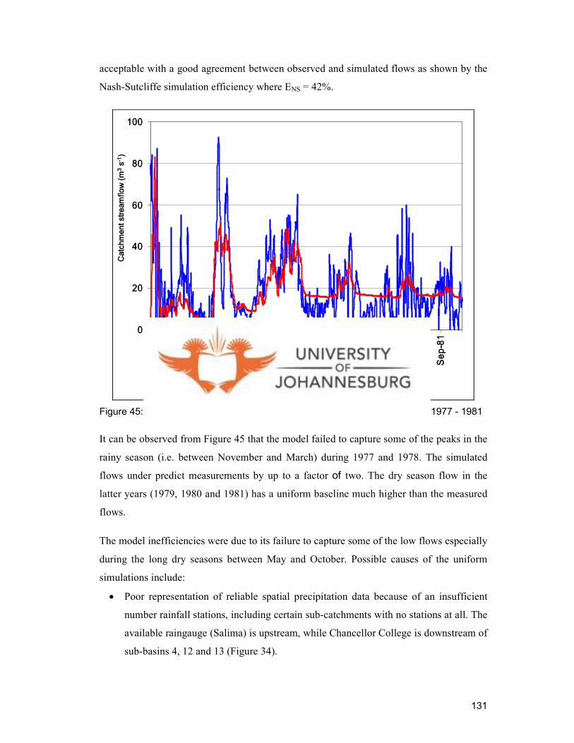
131
acceptable with a good agreement between observed and simulated flows as shown by the
Nash-Sutcliffe simulation efficiency where ENS = 42%.
Catchment streamflow (m3s-1)
0
20
40
60
80
100
Jan-77
May-77
Sep-77
Jan-78
May-78
Sep-78
Jan-79
May-79
Sep-79
Jan-80
May-80
Sep-80
Jan-81
May-81
Sep-81
Observed daily catchment streamflow (m3 s-1)
Simulated daily catchment streamflow (m3 s-1)
Catchment streamflow (m3s-1)
0
20
40
60
80
100
Jan-77
May-77
Sep-77
Jan-78
May-78
Sep-78
Jan-79
May-79
Sep-79
Jan-80
May-80
Sep-80
Jan-81
May-81
Sep-81
Observed daily catchment streamflow (m3 s-1)
Simulated daily catchment streamflow (m3 s-1)
Figure 45: Comparison of daily catchment streamflows for calibration period 1977 - 1981
It can be observed from Figure 45 that the model failed to capture some of the peaks in the
rainy season (i.e. between November and March) during 1977 and 1978. The simulated
flows under predict measurements by up to a factor of two. The dry season flow in the
latter years (1979, 1980 and 1981) has a uniform baseline much higher than the measured
flows.
The model inefficiencies were due to its failure to capture some of the low flows especially
during the long dry seasons between May and October. Possible causes of the uniform
simulations include:
• Poor representation of reliable spatial precipitation data because of an insufficient
number rainfall stations, including certain sub-catchments with no stations at all. The
available raingauge (Salima) is upstream, while Chancellor College is downstream of
sub-basins 4, 12 and 13 (Figure 34).

132
• The model was calibrated on the assumption that the soil comprised lumped clay-
loam. This soil generally has a low infiltration capacity. In reality, the basin consists
of a variety of soil units, which have not yet been mapped in sufficient detail or
precision.
• From a hydrological perspective, the occurrence of groundwater resources within the
Shire rift valley area is associated with low yielding weathered Precambrian
basement gneiss complex formations [Malawi Government, 2001]. The long
residence time of the groundwater may imply the existence of low hydraulic
gradients with subsequent low flow velocities, or low transmissivities due to the
nature of the aquifer material. Both theories seem to apply to the Shire River
catchment, as it is located in the Shire plain, which is characterised by flat
topography and clay-loam soils [Bath, 1980]. However, trends in groundwater levels
are due to many different factors and this requires more research, as data gathered by
the Department of Water Resources in Malawi on groundwater levels are
inconclusive.
• Possible error in the manipulation of the streamflow data from the inflow and
outflow measuring weirs to separate the Lake Malawi outflow form the catchment
contributions. As the latter flows are small compared to the Lake Malawi flow,
uncertainties are magnified in the adjusted set of measured streamflows.
Overall, the model was able to reproduce the main features of the streamflow in terms of
magnitude and seasonality. From the results, the model gives an adequate representation of
the water balance and outflow hydrographs at the basin outlet.
Daily validation
Validation runs were also performed to compare the daily measured (1984 – 1985) and
simulated catchment streamflows (Figure 46). The statistical evaluation of the simulated
catchment streamflow yielded ENS = 36% for the daily predictions. This model prediction
for the daily Shire River catchment streamflow is barely acceptable. The simulation flows
were able to follow the measured pattern but failed to simulate several of the highest flow
peaks in February, March and October 1984, and in February and March 1985. The model
gave a smooth outflow from May to November 1985, and appeared to be unresponsive to
minor fluctuations driving the measured flow. Uniform prediction of the catchment
streamflow in this period could be attributed to poor representation of rainfall data.

133
0
50
100
150
Jan-84
May-84
Sep-84
Jan-85
May-85
Sep-85
Catchment streamflow (m3 s-1)
Observed daily catchment streamflow (m3 s-1)
Simulated daily catchment streamflow (m3 s-1)
0
50
100
150
Jan-84
May-84
Sep-84
Jan-85
May-85
Sep-85
Catchment streamflow (m3 s-1)
Observed daily catchment streamflow (m3 s-1)
Simulated daily catchment streamflow (m3 s-1)
Figure 46: Comparison of daily catchment streamflow for validation period: 1984 - 1985
Results of land cover change test
In this section, results are presented for the test of substituting the 2002 land cover
classifications into the model, in place of the 1989 land cover, keeping climate input data
sets and all other parameters constant. Climatic data for the period 1977 to 1981 were used
for this comparison.
General patterns and trends of land cover change in the Shire River catchment between
1989 and 2002 suggest transition towards the degradation of woodlands and an increase in
subsistence agricultural land. The land cover mapping showed that 23% of the land was
covered by agricultural land in 1989. Subsistence agricultural area has increased by 18%,
occupying 41% of the study area in 2002. The increase in subsistence agricultural land
corresponds with the simultaneous decrease in vegetated areas. Summaries of the changes
in land cover distribution, showing the percentage of land cover for 1989 and 2002, are
presented in Chapter 2. Simulation runs were conducted on an annual, monthly and daily
basis to compare the modelling outputs using the 1989 and the 2002 land covers.

134
A comparison of the multi-year average annual streamflows generated using 1989 and
2002 land covers respectively is presented in Table 30, while Figure 47 presents mean
annual catchment streamflows. The 1989 land cover yielded mean annual water yield of
140 mm compared to 207 mm from the 2002 land cover. The maximum annual flow yield
for the 1989 land cover was 170 mm while in 2002 it was 318 mm (for the 1978
meteorological year). The total annual volume of water simulated increased by 47% with
the 2002 land cover.
Table 30: Parameters obtained from annual simulations for 1989 and 2002 land cover
Item 1989 land cover data 2002 land cover data
Mean annual water yield 140 mm 207 mm
Mean annual surface flow 82 mm 155 mm
Maximum annual mean flow (1978) 170 mm 318 mm
Simulated annual catchment streamflow, 1989 land cover (mm)
Simulated annual catchment streamflow, 2002 land cover (mm)
0
100
200
300
400
1977
1978
1979
1980
1981
Catchment annual streamflow (mm)
Simulated annual catchment streamflow, 1989 land cover (mm)
Simulated annual catchment streamflow, 2002 land cover (mm)
0
100
200
300
400
1977
1978
1979
1980
1981
Catchment annual streamflow (mm)
Figure 47: Simulated annual catchment streamflow for 1989 and 2002 land cover
Average annual catchment streamflows are directly related to land cover type, soil
characteristics and annual precipitation. In the study area, subsistence agricultural areas
have increased between 1989 and 2002, with most of the increase occurring in previously

135
vegetated areas of savanna and forest. Agricultural land has the highest potential for runoff
because the land is kept bare at the onset of the rainy season. AVSWATX simulates surface
run-off volumes and peak run-off rates for each HRU. Surface run-off is estimated with a
modification of the SCS curve number method [USDA-SCS, 1986]. In this study,
subsistence agricultural land has a curve number of 86 compared to 79 and 68 for savanna
and forest. The curve number is a dimensionless parameter indicating the runoff response
of a drainage basin. Changing land cover results in a different run-off curve number, which
could result in changes in rainfall run-off responses. High curve numbers signify high
surface run-off and low infiltration.
The total annual precipitation for 1977 to 1981 varies between 800 and 1500 mm with a
standard deviation of 23% from the long-term mean of 1090 mm. Annual variation of
rainfall from 1976 to 1981 from the long-term mean is shown in Figure 48. 1978 was an
excessively wet year (variance 47% above average), preceded by moderately high rainfall
in 1976 and a year of average rainfall in 1977. However, 1981 was a significantly dry year.
-40
-30
-20
-10
0
10
20
30
40
50
1976
1977
1978
1979
1980
1981Variance %
-40
-30
-20
-10
0
10
20
30
40
50
1976
1977
1978
1979
1980
1981Variance %
Figure 48: Rainfall variability between 1977 and 1981, referenced against long-term mean (1976 – 2002)
The catchment streamflow response analysis of the study area indicated that high rainfall
controls much of the increase in streamflow in the Shire River catchment. Taking the year
136
1976 as a lead in the period of intensive study, the recorded above average rainfall (Figure
48) is assumed to have contributed to saturated soil moisture storage. Any increments of
rainfall on already saturated soils contribute to increases in surface run-off, hence the
increase in streamflow in 1977 and 1978 (Figure 47). This trend is also related to 2002
land cover, which is dominated by subsistence agriculture, having recorded the highest
average annual catchment streamflow of greater than 300 mm in 1978, a year of 47%
above average rainfall.
The rainfall regime in 1979 is characterised by the onset of rainfall in mid-October,
average monthly rainfall below 200 mm in December, dry spells in January and average
monthly rainfall of less than 250 mm in March and April. This particular year corresponds
to decreasing total average annual streamflow of 135 mm for the 2002 land cover
compared to 112 mm for the 1989 land cover. In 1980 there was a slight increase in the
mean annual rainfall received (1 039 mm). However, two rainfall stations (Mangochi and
Balaka) had the lowest total rainfall (~550 mm and ~700 mm respectively). In this year,
there was an increase in catchment streamflow: 1989 streamflow is 23 mm lower than that
in 2002. This could be attributed to change in land cover from savanna to subsistence
agriculture and the increase in precipitation.
Another noticeable observation in the rainfall pattern is the decrease in simulated annual
catchment streamflow in 1981. The year was characterised by slightly below normal
precipitation with dry spells in January and low rains in February and March. Average
annual rainfall was ~750 mm. The study finds that the decrease in precipitation combined
with drying of the soils explains a gradual reduction in annual catchment streamflow (1979
– 1981) for the 2002 land cover. In contrast, for the 1989 land cover with higher forest
cover, the relative decrease is much smaller, possibly due to greater soil moisture retention
and increased infiltration.
Furthermore, the soil data for the study area indicates that the area is composed of the Soil
Conservation Service (SCS) hydrological group C. These soils are fine to very fine
textured and are generally shallow. They have a low to very low rate of water infiltration
when wet, which results in high run-off potential. Streamflow patterns in this catchment
are strongly influenced by the seasonal cycle of rainwater. Annual streamflows occur in
response to timing and degree of precipitation and the land cover characteristics.

137
To understand the flow processes during different seasons under different land cover
conditions, the average monthly streamflows were plotted for the wet and dry season and
compared. In the Shire River catchment, there are two seasons - wet weather occurs from
November to March and dry weather events occur between April and October. This two-
season climate creates significant differences in streamflow. Seasonal variations predicted
from the two land cover classifications (1989 and 2002) are presented in Figure 49.
From the modeling process, HRUs from the 1989 land cover are dominated by savanna,
while HRUs from the 2002 land cover are dominated by subsistence agriculture. The
average monthly streamflow shows differences between the two simulations (Figure 49).
For the 1989 land cover average monthly streamflow was in the range of 14 m3
s-1
to
31 m3
s-1
, while that of 2002 land cover data was between 16 m3
s-1
and 57 m3 s
-1. The
minimum average monthly catchment streamflow simulated for 1989 is 19 m3
s-1
, while
that of 2002 is 30 m3
s-1
. In general, storm events from the 2002 land cover yield both high
surface run-off rates and high total water volumes. The majority of peak flows occur
during the months of November to March, which is the rainy season in the study area.
0
20
40
60
80
100
Jan Mar May Jul Sep Nov Jan Mar May Jul Sep Nov
0
20
40
60
80
100
l min max h avg
1989 2002
Average monthly streamflow (m3s-1)
0
20
40
60
80
100
Jan Mar May Jul Sep Nov Jan Mar May Jul Sep Nov
0
20
40
60
80
100
l min max h avg
1989 2002
Average monthly streamflow (m3s-1)
Figure 49: Monthly mean, standard deviations and maxima of daily simulated catchment streamflows for 1989 and 2002 land cover simulations

138
The dominance of savanna landscapes in 1989 yielded relatively low average monthly
catchment streamflows. In comparison, the 2002 land cover, which is dominated by
agricultural land yielded high average monthly catchment streamflows.
A comparison of the multi-year daily catchment streamflows generated using 1989 and
2002 land covers respectively is presented in Table 31 and Figure 50
Table 31: Parameters obtained from daily simulations for 1989 and 2002 land cover
Item 1989 land cover data 2002 land cover data
Maximum daily flow 83 m3 s-1 154 m
3 s-1
Minimum daily flow 1 m3 s-1 3 m
3 s-1
Average daily flow 19 m3 s-1 30 m
3 s-1
Simulated daily catchment streamflow,1989 land cover (m3 s-1)
Simulated daily catchment streamflow, 2002 land cover (m3 s-1)
Catchment streamflow (m3s-1)
0
40
80
120
160
200
Jan-77
May-77
Sep-77
Jan-78
May-78
Sep-78
Jan-79
May-79
Sep-79
Jan-80
May-80
Sep-80
Jan-81
May-81
Sep-81
Simulated daily catchment streamflow,1989 land cover (m3 s-1)
Simulated daily catchment streamflow, 2002 land cover (m3 s-1)
Catchment streamflow (m3s-1)
0
40
80
120
160
200
Jan-77
May-77
Sep-77
Jan-78
May-78
Sep-78
Jan-79
May-79
Sep-79
Jan-80
May-80
Sep-80
Jan-81
May-81
Sep-81
Figure 50: Comparison of simulated daily catchment streamflows for 1989 and 2002 land cover data
The simulation results demonstrate that there are differences in the daily peak flows
between the 1989 land cover and 2002 land cover. The hydrograph generated for the 1989
land cover produced the highest daily peak flow of 83 m3
s-1
, whereas the 2002 land cover
produced the highest daily peak of 154 m3
s-1
(Figure 50). However, an anomaly was
observed during the dry season of 1979 to 1981. The model failed to capture the dry season

139
variations for both the 1989 and 2002 land cover, which simulated a uniform baseline.
Possible reasons have been outlined in Section 4.3.2 as these model inefficiencies were
also observed during model calibration within this study. The daily catchment streamflow
analysis for each year of the study period indicates high flow peaks at the beginning of the
rainy season, implying that rainfall on saturated soils causes much of the flow. Saturated
soils are efficient at producing more streamflow. High surface flow signifies low
infiltration during the rainy season and consequently diminishes ground water
replenishment during the dry season.
Total streamflow is composed of surface run-off and baseflow (lateral flow and shallow
ground water discharge to streams). Comparisons were also done to evaluate differences in
surface flow and baseflow from different land cover types classified from the 1989 and the
2002 land cover data sets. Between 1989 and 2002, dominant land cover changes were
observed in sub-basins 2, 4, 5, 6, 7, 9, 11, 12 and 13, while sub-basins 1, 3, 8 and 10 did
not change (Figure 40). Table 32 and Table 33 show differences in surface run-off,
baseflow and the percentage changes.
Table 32: Surface run-off simulated from 1989 and 2002 land cover
Simulated average annual surface run-off (mm)
Change (mm)
Percentage change (%) Sub-basin
1989 2002
1 51 51 0 0
2 42 149 107 255
3 Reservoir 0 0 0
4 51 175 124 243
5 39 147 108 277
6 52 175 123 237
7 43 4 -39 -91
8 52 52 0 0
9 42 149 107 255
10 149 149 0 72
11 88 235 147 167
12 11 267 256 2327
13 88 235 147 167
Entire Shire River catchment
82 155 73 89
The highest annual surface run-off of 267 mm was generated in densely populated
settlement areas in sub-basin 12. The dominant land cover in sub-basin 12 was forest in

140
1989 and had changed to subsistence agriculture in 2002. Thus, surface run-off increased
by 2 327% from 11 mm to 267 mm, while baseflow decreased by -48% from 190 mm to
98 mm. Subsistence agricultural land is characterised by scattered grasslands, used for
communal grazing during the dry season. At the onset of the rainy season, most of these
fields are bare soil that have been prepared for planting, or denuded by grazing. Most of
the run-off generated in the cultivated and grazing lands constitutes storm flow, especially
at the beginning of the rainy season between November and January.
Table 33: Baseflow simulated from 1989 and 2002 land cover
Simulated average annual baseflow (mm)
Change (mm)
Percentage change (%) Sub-basin
1989 2002
1 93 93 0 0
2 66 30 -36 -55
3 Reservoir 0 0 0
4 90 55 -35 -39
5 83 57 -26 -46
6 100 63 -37 -37
7 70 84 14 20
8 99 99 0 0
9 65 29 -36 -55
10 29 29 0 0
11 101 52 -49 -49
12 190 98 -92 -48
13 101 58 -43 -43
Entire Shire River catchment
59 74 15 25
Similar observations have been noted in sub-basins 2, 4, 5, 6, 9, 11 and 13 where dominant
land cover has changed from savanna shrubs (RNGB) to subsistence agriculture (AGRL).
Under the simulated conditions of a fixed climatic scenario, with only the measured land
cover changes inserted, simulated surface run-off increased by 255%, 243%, 277%, 237%,
255%, 167% and 167% in sub-basins 2, 4, 5, 6, 9, 11 and 13 respectively. Proportionately,
baseflow decreased by -55%, -39%, -46%, -37%, -55%, -49% and -43% respectively. The
high variability between sub-basins indicates the need to segment catchments into these
smaller units, to understand the full extent of land cover changes.
Large portions of the original woodlands have been cleared. This is due to expansion of
agricultural land for food production, fuelwood and construction. The majority of
141
subsistence farmers in Malawi practice traditional methods of cultivation. Soil and water
conservation technologies are not practised, and generally the adoption rate for most land
husbandry technologies is low [Malawi Government, 2001]. Hence, when agricultural land
becomes impoverished, it is common practise to clear fresh forest or savanna.
With less plant cover, more rainfall runs off the surface rather than infiltrates into the
ground. If the run-off from a storm is greater, the chance of the flow exceeding the stream
capacity and causing flooding increases. In addition, water that runs off does not have a
chance to recharge groundwater. Groundwater flows slowly into streams, usually over a
period of months, providing steady baseflow (flow in streams in times without rainfall).
This sequence of events is a cause of concern as it makes a major difference to stream
characteristics and health, causing increased streambank erosion due to higher peak flows
during the rainy season and periods of very low flow due to the decreased baseflow during
the dry season.
It is notable that the dominant land cover in sub-basin 7 changed from savanna shrubs
(RNGB) to forest (FRSD) in 2002. Sub-basin 7 is located within the valley of the Shire
River, which represents the smallest sub-basin (79 km2). The change to dominant forest for
the 2002 land cover yielded the minimum annual surface run-off (dropping from 43 mm to
4 mm), proportionate with high baseflow (rising from 70 mm to 84 mm) compared to the
other sub-basins. Changes in land cover may have a significant effect on available water
resources and could determine the amount of water that flows in rivers. Forested areas
have good infiltration, a large baseflow component and small storm flow. Forests absorb
water, retain it, release it slowly, and have low erosion rates [Calder, 2000].
Comparable studies have been done to assess the ability of the SWAT model to analyse the
effects of land cover changes on streamflow. Tadele et al. [2007] investigated land cover
dynamics and its impacts on streamflow at Hare River watershed, southern Rift Valley
Lakes Basin, Ethiopia. In order to asses the variability of streamflow due to the land cover
dynamics from 1975 to 2004, the AVSWATX model was run using two land cover maps
(1992 and 2004), while all the other input variables were similar for both simulations. It
was identified that mean monthly discharge for wet months had increased by 13% while in
the dry season they decreased by up to 31% during the 1992 – 2004 period due to land
cover change.

142
A critical aspect of this study has been to establish the links between extensive land cover
change and hydrological responses. Simulations were performed by substituting 1989 land
cover with 2002 land cover classifications while keeping climate constant. Large portions
of the Shire River catchment have been transformed from savanna and forest to subsistence
agricultural land between 1989 and 2002. Simulation results revealed that streamflow
patterns in this catchment have been strongly influenced by the land cover changes that
have occurred over the relatively short period of thirteen years.
Further, it has been demonstrated that subsistence agricultural areas generated higher
surface run-off than savanna and forest areas. Areas dominated by subsistence agriculture
are generally bare at the onset of the rainy season, and hence less effective in reducing run-
off. Higher surface run-off and less infiltration are not conducive of sustainability for rural
agriculture as they erode fertile surface soils and make areas more vulnerable to periods of
drought. The use of small-scale irrigation agriculture to combat cyclical food insecurity
may be hampered by the lack of perennial water flows.
Additionally, water in the Shire River is almost totally allocated to hydro-electric power
stations in the mid-catchment, irrigation schemes in the lower-catchment and domestic
purposes [Malawi Government, 2001]. Water shortages during drought periods may
therefore increase water contestation among different users.
This study has also established that increasing forest and savanna area yields less surface
run-off compared to that of areas under subsistence agriculture. There is also an increase in
baseflow, which contributes to ground water replenishment. Thus, forest areas are the
preferred land cover type with regard to the sustainability of the water balance for water
resources management.
4.3.3 Scenario outcomes
Simulations were performed using three scenarios, which were compared to the baseline
case. The baseline case was taken as the simulation using measured climate (1977 to 1981)
and the 2002 land cover image. The scenarios are the case of bounding scenarios (which
were used to test the sensitivity of AVSWATX in simulating changes in land cover
characteristics), land degradation and land conservation specified in Table 25 and Table
26 respectively. The hydrological responses at the outlet thus simulated were compared to
the baseline case in terms of average annual catchment streamflows, surface run-off and
baseflows.

143
Bounding scenarios
Changes in land cover cause changes in curve number, the internal model parameter that
determines the partitioning of precipitation into surface flow and percolation. Evaluation of
model sensitivity, through the trial of extreme land cover scenarios, revealed the maximum
degree and patterns of interaction between changes in land cover and modelled
hydrological responses.
The results of the two extreme scenarios are compared to the baseline case (Table 34).
Total deforestation of the entire land surface of the catchment generated a total water yield
of 463 mm a-1
, compared to 397 mm a-1
for the reference scenario. In the case of total
deforestation, there is increase in surface flow of 437 mm a-1
compared to 322 mm a-1
, and
a decrease in baseflow of 26 mm a-1
in comparison with 74 mm a-1
for the reference
scenario. Bare areas have a strong effect by promoting rapid run-off and thereby reducing
percolation. Ground storage is reduced and surface direct evaporation enhanced.
For total forestation, total water yield reduced to 308 mm a-1
. In the case of total land cover
change to forest, there is a decrease in surface flow from 322 mm a-1
to 195 mm a-1
and
increase in baseflow from 74 mm a-1
to 113 mm a-1
. Forests absorb most of the
precipitation hence there is increased interception, percolation and evapotranspiration,
rather than prompt streamflow.
Results of this sensitivity analysis show the maximum changes that could be expected from
extreme changes in land cover, and hence bounding conditions for the further scenario
modelling. The model behaves as expected, with bare land increasing prompt run-off and
reducing percolation, and conversely reducing run-off and total yield for full forestation.
Table 34: Simulation results from bounding cases scenarios
Total water yield (mm) Surface flow (mm) Baseflow (mm)
2002 land cover 397 322 74
Total change to bare soil 463 437 26
Total change to forest 308 195 113
Land degradation
Simulation runs were performed using land cover from scenarios termed land degradation,
which represents an unfavourable scenario with accelerated land cover change with
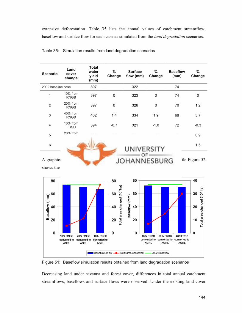
144
extensive deforestation. Table 35 lists the annual values of catchment streamflow,
baseflow and surface flow for each case as simulated from the land degradation scenarios.
Table 35: Simulation results from land degradation scenarios
A graphical representation of the baseflow results is shown in Figure 51 while Figure 52
shows the surface flow results.
0
20
40
60
80
10% RNGB
converted to
AGRL
20% RNGB
converted to
AGRL
40% RNGB
converted to
AGRL
Baseflow (mm)
0
20
40
60
80
0
20
40
60
80
10% FRSD
converted to
AGRL
20% FRSD
converted to
AGRL
40%FRSD
converted to
AGRL
Baseflow (mm)
0
10
20
30
40
Baseflow (mm) Total area converted 2002 Baseflow
Total area changed (103 ha)
Total area changed (103ha)
0
20
40
60
80
10% RNGB
converted to
AGRL
20% RNGB
converted to
AGRL
40% RNGB
converted to
AGRL
Baseflow (mm)
0
20
40
60
80
0
20
40
60
80
10% FRSD
converted to
AGRL
20% FRSD
converted to
AGRL
40%FRSD
converted to
AGRL
Baseflow (mm)
0
10
20
30
40
Baseflow (mm) Total area converted 2002 Baseflow
Total area changed (103 ha)
Total area changed (103ha)
Figure 51: Baseflow simulation results obtained from land degradation scenarios
Decreasing land under savanna and forest cover, differences in total annual catchment
streamflows, baseflows and surface flows were observed. Under the existing land cover
Scenario Land cover change
Total water yield (mm)
% Change
Surface flow (mm)
% Change
Baseflow (mm)
% Change
2002 baseline case 397 322 74
1 10% from RNGB
397 0 323 0 74 0
2 20% from RNGB
397 0 326 0 70 1.2
3 40% from RNGB
402 1.4 334 1.9 68 3.7
4 10% from FRSD
394 -0.7 321 -1.0 72 -0.3
5 20% from FRSD
396 -0.3 325 -0.3 70 0.9
6 40% from FRSD
397 0.2 327 0.3 70 1.5

145
(reference scenario, 2002), the annual catchment streamflow observed was 397 mm, with
baseflow making up to 19% and the remaining 81% from surface flow. In terms of
absolute mean annual changes between the reference state and the scenarios, decreasing
forest areas by different magnitudes increases surface flow and decreases baseflow and
total water yield at the outlet.
A 10% decrease in the savanna areas increases total water yield from 397 mm a-1
to
402 mm a-1
. With a 10% decrease in savanna, baseflow remains at 74 mm a-1
while surface
flow was 323 mm a-1
with minor difference from the reference scenario at 322 mm a-1
.
However, decreasing savanna areas by 20% produces an increase in total water yield and
surface flow but a decrease in baseflow. Total water yield increased from 397 mm a-1
to
402 mm a-1
while surface flow increased from 322 mm a-1
to 334 mm a-1
. A minor
decrease in baseflow has been observed once savanna was decreased by 20%. The
conversion of savanna into subsistence agriculture does not cause considerable changes in
the macro scale basin. The reason for this may be the similarity of the characteristics of
both land cover forms under tropical natural conditions. Savanna vegetation has scattered
trees and is deciduous during the dry season. Thus, a considerable amount of land is
exposed, similar to subsistence agricultural land.
0
100
200
300
400
10% RNGB
converted to
AGRL
20% RNGB
converted to
AGRL
40% RNGB
converted to
AGRL
Surface flow (mm)
0
20
40
60
80
Surface flow (mm) Total area converted 2002 Surfaceflow
0
100
200
300
400
10% FRSD
converted to
AGRL
20% FRSD
converted to
AGRL
40%FRSD
converted to
AGRL
Surface flow (mm)
0
20
40
60
80
Total area changed (103ha)
Total area changed (103ha)
0
100
200
300
400
10% RNGB
converted to
AGRL
20% RNGB
converted to
AGRL
40% RNGB
converted to
AGRL
Surface flow (mm)
0
20
40
60
80
Surface flow (mm) Total area converted 2002 Surfaceflow
0
100
200
300
400
10% FRSD
converted to
AGRL
20% FRSD
converted to
AGRL
40%FRSD
converted to
AGRL
Surface flow (mm)
0
20
40
60
80
Total area changed (103ha)
Total area changed (103ha)
Figure 52: Surface flow simulation results obtained from land degradation scenarios
A 40% decrease in forest yielded total water yield of 397 mm a-1
, not different from the
reference scenario. Slight decreases in baseflow ranging from 70 mm a-1
to 72 mm a-1
have
been observed with an increase in the magnitude of deforestation. For example, a 10%
decrease in forest results in a decrease in baseflow from 74 mm a-1
to 72 mm a-1
, while a

146
40% decrease in forest produces a decrease in baseflow 70 mm a-1
. Surface flows were
observed to be increasing as forestland is reduced. For example, a 40% decrease in forest
increases surface flow from 322 mm a-1
to 327 mm a-1
.
The relative effect of woodland (savanna and forest) reduction (expressed as percentages)
on the annual water balance is compared to that of subsistence agriculture. The 10%
decrease in forest reduces total water yield by 0.7%, whereas a 20% reduction of forest
leads to a decline of water yield by 0.3%. Overall, the strongest relative impact can be
observed in the amount of surface run-off. Decreasing land under savanna cover by 20%
increases surface flow by 4% while decreasing forest by 40% increases surface flow by
2%. This is due to the increase in land under subsistence farming. The absence of trees and
shrubs implies a minimum in surface evapotranspiration and, consequently, a maximum in
run-off. The soil is less protected against raindrop impact under agriculture since after
harvesting and shortly after sowing, when the plants do not cover the soil completely.
Land conservation scenario
Simulation runs were also performed for land cover scenarios termed land conservation,
which represents the creation of a greener environment through management and re-
forestation. Table 36 lists the annual volumes of catchment streamflow, baseflow and
surface flow for each scenario as simulated from land conservation scenarios. The
conversion of subsistence agricultural land into woodlands (savanna and forests) leads to
changes in the water balance.
Table 36: Simulation results obtained from land conservation scenarios
Scenario Land cover change
Total water yield (mm)
% Change
Surface flow (mm)
% Change
Baseflow (mm)
% Change
2002 baseline 397 322 74
7 20% to RNGB 373 -6 284 -8 89 -12
8 40% to RNGB 332 -16 217 -22 115 -33
9 20% to FRSD 398 0.5 298 0.2 99 -8
10 40% to FRSD 397 0.2 173 0.6 225 -46
11 20% both RNGB and FRSD
371 -12 192 -16 158 -41
12 40% both RNGB and FRSD
350 -6 161 -9 210 -50

147
A 40% increase in forest increases total water yield from 397 mm a-1
to 398 mm a-1
.
However, the proportion of water infiltrating increases from 74 mm a-1
to 225 mm a-1
while surface flow decreased from 322 mm a-1
to 173 mm a-1
. Slight increases in baseflow
have been observed with a 20% increase in forest, when baseflow increases from 74 mm a-
1 to 99 mm a
-1. Surface flows were observed to decrease as savanna expands. For example,
a 40% increase in savanna, results in a drop in total water yield from 397 mm a-1
to
332 mm a-1
. This reduction is associated with an increase in baseflow from 74 mm a-1
to
115 mm a-1
. Increasing the areas of forest and savanna decreases water yield and surface
flow, and increases baseflow. For instance, an increase of 20% decreases total water yield
to 371 mm a-1
while a 40% increase decreases water yield to 350 mm a-1
compared to
397 mm a-1
from the reference scenario. The reduction of the mean annual flow results in a
decreasing surface flow during the rainy season with a simultaneous increase in baseflow.
Graphical representations of the changes for baseflow are shown in Figure 53, while for
surface flow they are presented in Figure 53 while for surface flow they are presented in
Figure 54.
0
50
100
150
200
250
20% AGRL converted to
FRSD
40% AGRL converted to
FRSD
Baseflow (mm)
-100
-80
-60
-40
-20
0
Baseflow (mm) 2002 Baseflow Total area converted
0
50
100
150
20% AGRL converted to
RNGB
40% AGRL converted to
RNGB
Baseflow (mm)
-150
-100
-50
0
Total area changed (103ha)
Total area changed (103ha)
0
50
100
150
200
250
20% AGRL converted to
FRSD
40% AGRL converted to
FRSD
Baseflow (mm)
-100
-80
-60
-40
-20
0
Baseflow (mm) 2002 Baseflow Total area converted
0
50
100
150
20% AGRL converted to
RNGB
40% AGRL converted to
RNGB
Baseflow (mm)
-150
-100
-50
0
Total area changed (103ha)
Total area changed (103ha)
Figure 53: Baseflow simulation results from land conservation scenarios

148
Surface flow (mm) Total area converted 2002 Surfaceflow
0
100
200
300
400
20% AGRL converted to
FRSD
40% AGRL converted to
FRSD
Surface flow (mm)
-100
-50
0
0
100
200
300
400
20% AGRL converted to
RNGB
40% AGRL converted to
RNGB
Surface flow (mm)
-100
-50
0
Total area changed (103ha)
Total area changed (103 ha)
Figure 54: Surface flow simulation results from land conservation scenarios
Increasing woodland (both savanna and forest) has a profound effect on the annual water
balance when compared to the reference scenario (Figure 55). The 20% increase in the
forest increases total water yield by 0.5% whereas an additional 20% increase of forest
leads to a decline in water yield by 0.2%. This could be due to the small amount of land
initially under forest.
0
100
200
300
400
20% AGRL converted to
FRSD and RNGB
40% AGRL converted to
FRSD and RNGB
Surface flow (mm)
-200
-150
-100
-50
0
Surface flow (mm) Total area converted 2002 Surfaceflow
0
50
100
150
200
250
20% AGRL converted to
FRSD and RNGB
40% AGRL converted to
FRSD and RNGB
Baseflow (mm)
-250
-200
-150
-100
-50
0
Baseflow (mm) 2002 Baseflow Total area converted
Total area converted (103ha)
Total area converted (103ha)
0
100
200
300
400
20% AGRL converted to
FRSD and RNGB
40% AGRL converted to
FRSD and RNGB
Surface flow (mm)
-200
-150
-100
-50
0
Surface flow (mm) Total area converted 2002 Surfaceflow
0
50
100
150
200
250
20% AGRL converted to
FRSD and RNGB
40% AGRL converted to
FRSD and RNGB
Baseflow (mm)
-250
-200
-150
-100
-50
0
Baseflow (mm) 2002 Baseflow Total area converted
Total area converted (103ha)
Total area converted (103ha)
Figure 55: Baseflow and surface flow simulation results from land conservation scenarios
Generally, the strongest relative impact can be observed in the amount of surface flow.
Increasing land under savanna cover by 40% decreases surface flow by 33%, while
increasing the savanna area by 20% decreases surface flow by 12%. Differences in surface
flow and baseflow were also observed with increases of both forest and savanna areas by

149
40% and 20% respectively. Reductions in surface flow of 50% and 40% were observed
respectively. This is due to the decrease in land under subsistence farming. Baseflow
increases and surface flow decreases are due to the higher interception of forests and
savanna woodlands in comparison to maize and legumes. Observational and experimental
studies have established that forests consume more water during evapotransipiration than
any other forms of land cover [Dingman, 2008]. Large reductions of the river discharge
and therefore a considerable increase of water retention in the catchment would occur only
in the case of forestation of large areas. Therefore, depending on the magnitude of
percentage change in forest cover, forestation would decrease average and dry-season
streamflow.
Seasonal variability
Streamflow and baseflow vary significantly during the year because of seasonal weather
changes, coupled to variations in land cover characteristics. The seasonal water balance
analyses suggest that when the river discharge increases in the Shire River in November-
March, the amount of maximum catchment streamflow decreases with increase in
reforested areas (Figure 56). In the scenario where only savanna replaces subsistence
agricultural land by 20% (scenario 7), the maximum catchment streamflow is 259 m3 s
-1.
An increase of 40% yielded a maximum catchment streamflow of 216 m3 s
-1 compared to a
maximum catchment streamflow of 281 m3 s
-1 for the 2002 land cover. On average, when
there is a 20% savanna increase, monthly catchment streamflow ranges from 13 m3 s
-1 to
151 m3 s
-1, while a 40% savanna increase yields monthly catchment streamflow averages
ranging between 17 m3 s
-1 and 124 m
3 s
-1. Average monthly flows for the reference
scenario range from 12 m3 s
-1 to 166 m
3 s
-1. Overall, the seasonal pattern of streamflow
responds to the precipitation pattern, with greatest streamflow and baseflow occurring in
the November to March period.

150
Average monthly streamflow (m3s-1)
0
50
100
150
200
250
300
Sc7
Jan
Sc7
Mar
Sc7
May
Sc7
Jul
Sc7
Sep
Sc7
Nov
Sc8
Jan
Sc8
Mar
Sc8
May
Sc8
Jul
Sc8
Sep
Sc8
Nov
0
50
100
150
200
250
300
l min max h Reference avg
Average monthly streamflow (m3s-1)
0
50
100
150
200
250
300
Sc7
Jan
Sc7
Mar
Sc7
May
Sc7
Jul
Sc7
Sep
Sc7
Nov
Sc8
Jan
Sc8
Mar
Sc8
May
Sc8
Jul
Sc8
Sep
Sc8
Nov
0
50
100
150
200
250
300
l min max h Reference avg
Figure 56: Monthly mean, standard deviations and maxima of daily simulated catchment streamflows for 2002 land cover scenario 7 and 8 simulations
The model was used also to evaluate the potential effects of increasing forest areas in
regions initially covered by subsistence agriculture. The seasonal water balance analyses
shows that when land under forest vegetation increases, dry season flow increases and wet
season peak flow decreases compared to the reference land cover scenario (Figure 57). The
maximum catchment streamflow decreases and there is an increase in the scale of
reforestation. When forest areas were increased by 20% (scenario 9), catchment
streamflow yielded a mean monthly maximum catchment streamflow of 276 m3 s
-1 in
February, while a 40% forest increase (scenario 10) yielded 230 m3 s
-1. On average, with a
20% forest increase, monthly catchment streamflow averages range from 16 m3 s
-1 to
159 m3 s
-1, while a 40% forest increase yields monthly catchment streamflow averages
between 31 m3 s
-1 and 123 m
3 s
-1. Average monthly flows for the reference scenario range
from 12 m3 s
-1 to 166 m
3 s
-1. A comparison of the water balance components over the two
seasons for the different reforestation magnitudes indicates that the contribution of
baseflow during the dry season is high, while maximum catchment streamflow is
considerably lower than the reference scenario.

151
0
50
100
150
200
250
300
Sc9
Jan
Sc9
Mar
Sc9
May
Sc9
Jul
Sc9
Sep
Sc9
Nov
Sc10
Jan
Sc10
Mar
Sc10
May
Sc10
Jul
Sc10
Sep
Sc10
Nov
0
50
100
150
200
250
300
l min max h Reference avg
Average monthly streamflow (m3s-1)
0
50
100
150
200
250
300
Sc9
Jan
Sc9
Mar
Sc9
May
Sc9
Jul
Sc9
Sep
Sc9
Nov
Sc10
Jan
Sc10
Mar
Sc10
May
Sc10
Jul
Sc10
Sep
Sc10
Nov
0
50
100
150
200
250
300
l min max h Reference avg
Average monthly streamflow (m3s-1)
Figure 57: Monthly mean, standard deviations and maxima of daily simulated catchment streamflows for 2002 land cover, scenario 9 and 10 simulations
Impact simulations were carried out for the analyses of the current situation (reference
scenario) considering land cover changes towards land conservation. Scenario 11 and 12
correspond to conversion of potentially vulnerable areas (subsistence agricultural land) into
forest and savanna woodlands. Figure 58 shows the simulation results of the seasonal
variations under 20% and 40% increases in both forest and savanna land cover scenarios.
During the low flow period from April to October, dry season flow increases compared to
the reference land cover scenario when there is large scale reforestation. On average, with
a 20% increase in forest and savanna, monthly averages range from 24 m3 s
-1 to 118 m
3 s
-1,
while a 40% forest and savanna increase yields monthly flow averages between 32 m3 s
-1
and 111 m3 s
-1. Average monthly flows for the reference scenario range from 12 m
3 s
-1 to
166 m3 s
-1. Seasonal differences are also detected in terms of maximum flows during the
wet season. The reference land cover yields a maximum flow of 281 m3 s
-1 while
reforesting land by 20% and 40% yields flows of 206 m3 s
-1 and 193 m
3 s
-1 respectively.
Large-scale reforestation can significantly reduce average annual water flow in rivers and
affect the seasonal distribution flow.

152
0
50
100
150
200
250
Sc11
Jan
Sc11
Mar
Sc11
May
Sc11
Jul
Sc11
Sep
Sc11
Nov
Sc12
Jan
Sc12
Mar
Sc12
May
Sc12
Jul
Sc12
Sep
Sc12
Nov
0
50
100
150
200
250
l min max h avg Reference
Average monthly streamflow (m3s-1)
0
50
100
150
200
250
Sc11
Jan
Sc11
Mar
Sc11
May
Sc11
Jul
Sc11
Sep
Sc11
Nov
Sc12
Jan
Sc12
Mar
Sc12
May
Sc12
Jul
Sc12
Sep
Sc12
Nov
0
50
100
150
200
250
l min max h avg Reference
Average monthly streamflow (m3s-1)
Figure 58: Monthly mean, standard deviations and maxima of daily simulated catchment streamflows for 2002 land cover, scenario 11 and 12 simulations
Similar studies have been performed with the SWAT model to simulate the hydrological
behaviour of catchment areas using hypothetical land cover scenarios [Eckhardt et al.,
2003; Forher et al., 2001; Huisman et al., 2004] For example, simulations were run to
analyse the effects of the hydrological response of a catchment to different land use options
(Fohrer, 2001). In this study, SWAT was applied for the Dietzhölze watershed in Germany,
with two land use scenarios using the 1992 land cover data as a reference scenario. The
model results showed that the decrease of forest and corresponding increase in grassland
increased the peak flow rate (from 72 mm a-1
to 126 mm a-1
), and thus increases the risk of
flooding. The expansion of grassland and cropland in formerly forested areas increased
baseflow by 2%. A minor increase in run-off was observed due to the additional cropland
proportion. Baseflow decreased by 8% and total streamflow was reduced by 14 mm a-1
in
comparison with the actual 1994 land use.
Comprehensive hydrological models like AVSWATX can thus give valuable information,
which can be incorporated in catchment management studies. The hydrological processes
(surface flow, baseflow and infiltration) are largely driven by the nature and density of
land cover and the type of land cover over a catchment. In this study, the applicability of
AVSWATX in different contexts of catchment management has been explored. The capacity
to predict the effects of future land cover changes is very important for future use and
management strategies in the Shire River catchment.

153
4.4 Conclusion
The spatial semi-distributed hydrological model, AVSWATX, in combination with GIS, has
been applied to the upper Shire River basin, the largest surface water resource in Malawi.
The model was used to simulate water balance and river flows using digital elevation; soil
and land cover data; and five years (1977 to 1981) of observed daily precipitation,
temperature, wind speed and relative humidity data. The model was successful in
reproducing streamflow within the limits of observational and modelling errors. The study
showed that surface-water model parameters are sensitive and have physical meaning,
especially the CN2, ESCO and SOL_AWC. From the results obtained, it has been
concluded that the model has relatively high confidence and gives a good representation of
the water balance and outflow hydrographs at the basin outlet. The model performance
(1977-1981) using the Nash-Sutcliffe efficiency for reproducing catchment streamflow is
86% and 42% for monthly and daily calibrations respectively.
The fact that the optimal evaluation results have not been achieved could be a result of the
limited global input parameters and the complexity of optimisation of some of these
parameters. The lack of high resolution DEM, soil maps and a dense network of
precipitation and weather input data stations for the Shire River basin compromised the
simulations especially for the daily runs. There was generally an underestimation of
baseflows, especially during the dry months, which could be attributed to limited detailed
spatial rainfall data availability. Low yielding weathered Precambrian basement gneiss
complex formations within the Shire rift valley region could also have affected ability of
the model to simulate the lowest baseflows. In spite of these limitations, the model
captured the dynamic of flow generation well, with surface run-off dominating during the
rainy season and shallow aquifer contributing during the dry months. In addition, the
AVSWATX model provided insight in the main flow processes during the year. The model
appears to be suitable for application to large tropical river basins with ungauged stations.
The use of ArcView GIS with the AVSWATX model enabled the performance of quicker
hydrological analyses, especially for large basins, using the semi-distributed model.
In the present work, the influences of hypothetical land cover change characteristics upon
the hydrological processes that precipitation undergoes on delivery to the land surface were
also investigated. All of the flow parameters discussed – streamflows, baseflow and
surface flow are affected by the amount of plant cover, which is influenced by density and
spatial distribution. The results of the analysis have highlighted the sensitivity of surface

154
flow and baseflow in response to the suggested decrease in woodlands. Consequently,
seasonal variations in river discharge have been associated with decreased infiltration
during the wet season, which can affect the streamflow during the dry season by inhibiting
ground water recharge. Evaluation of effects of forestation on flow variability has
demonstrated that land covered with forest decreases surface flow and increases ground
water recharge.
Hydrological processes are an integrated indicator of catchment conditions, and changes in
land cover may affect the overall health and functioning of a catchment. An understanding
of temporal changes and trends in streamflow and the proportion of surface flow and
baseflow is critical for directing efforts in managing land cover and improving agricultural
practices. Exploring land cover change scenarios provides a wider applicability for
assessing the effects of land cover or land management change and hydrological responses.
If policies for land use management are to be established, methods must be available to
demonstrate that change has occurred, and what the nature and source of the change
involve. This method of evaluating of the effects of land management on water availability
can be used when planning for sustainable land and water resources management.

155
Chapter 5
5 CONCLUSION AND RECOMMENDATIONS
This final chapter summarises the main research findings and recommends future
investigations to advance the field of physically based hydrological modelling for the
management of water resources in Malawi.
5.1 Conclusion
The Shire River provides an important water resource for the socio-economic development
of Malawi. Currently, there is concern about the growing competition for water resources
within the catchment. With increasing human activities, it is important to understand
interactions between hydrological regimes and associated land use, and land cover change
in the catchment. Such interventions can be achieved by integrating land use planning and
water resources management. Therefore, a comprehensive assessment of the spatial and
temporal distribution of land cover change, as well as impacts on the land - hydrological
processes are required to resolve present problems and avoid potential crises in future
water resource allocations. At national level, results of this study can be used to improve
land use management to achieve sustainable water utilisation in the Shire River catchment.
This study was based on the hypothesis that unsustainable changes in land cover due to
human activities are significantly altering aggregate catchment conditions, giving rise to
long-term, potentially irreversible changes in river flow characteristics. The study was
aimed at answering the question: What are the effects of significant land cover changes
over the past two decades on river flow characteristics that are important for water
resources, environmental functioning and hydrological processes within the Shire River
catchment? Land cover changes associated with growing human populations and expected
changes in climatic conditions are likely to accelerate alterations in hydrological
phenomena and processes on various scales. Consequently, these changes significantly
influence the quantity and quality of water resources for nature and human society. This
aim was further pursued in the context of developing integrated land use planning and
water resources management in Malawi.
The basis of this research comprised multi-temporal classification of Landsat satellite
imagery (1989 and 2002) to provide a recent perspective of land cover types and changes
within the Shire River catchment of Malawi. Results from this study indicate successfully

156
the synergy between Landsat data, vector data and detailed ground information in mapping
land cover features. It was found that by integrating contextual information and ancillary
data, discrimination of heterogeneous land cover classes dominant in savanna woodlands
was improved. Eight land cover classes, comprising cultivated or grazing lands,
grasslands, savanna shrubs, marshes, woody open, woody closed, built-up areas and fresh
water, were mapped for the Shire River catchment, with an overall accuracy of 87%. The
land cover maps generated have compatible digital formats, hence they can be applied
easily to a variety of future GIS applications. Additional themes can be incorporated as
more resource information becomes available, or as new management needs are identified.
To map the land cover variables, a hierarchical legend structure determined by the Food
and Agriculture Organisation (FAO) Land Cover Classification System (LCCS)
(FAO/LCCS) was used [Di Gregorio and Jansen, 2005]. LCCS was used as a basis for the
classification to achieve legend harmonisation within Africa and on a global scale.
Flexibility of the hierarchical system allowed incorporation of digital elevation objects, soil
and underlying geological features as well as other available geographical datasets. By
integrating contextual information and ancillary data, classification accuracy was
improved. The new FAO/LCCS classification is also internally consistent, allowing
scalability and updatability that can be used at different scales and different levels of detail
to discriminate land cover features. In addition to compatibility with the FAO/LCCS, the
derived land cover maps have provided recent and improved classification accuracy, added
thematic detail compared to the most recent existing 1992 land cover maps for Malawi.
Accurate and up-to-date land cover change information is necessary to provide an
improved spatial representation of land cover data for hydrological parameterisation and
modelling, including other applications, to reflect actual land cover conditions.
Results from the mapping were used to analyse land cover change between 1989 and 2002.
Performing change detection analysis for the Shire River catchment revealed distinct
patterns in land cover change regarding disturbance and fragmentation of the landscape.
Carrying out this study in Malawi, therefore, has provided valuable information to evaluate
land cover dynamics and the percentage of cover change in the catchment. The change
analysis showed an increase of 4 622 ha (7.9%) in cultivated or grazing lands emanating
from declining natural vegetated areas. The main driving factors are subsistence
agricultural expansion and demand for wood resources. As agriculture continues to play a

157
dominant role in land cover conversion and degradation from Brachystegia woodlands,
more open and drier vegetation formations will continue to evolve. To this end, it is
apparent that the rapid increase in cultivated areas within the catchment will not only
decrease the amount of forests and vegetated areas but also increase run-off potential. This
process will diminish the overall quality and quantity of water resources. The mapping and
change detection exercise has not only characterised the landscape but will develop our
understanding of how to manage it more effectively. Distinguishing and quantifying where
potentially risky land cover changes occur is critical to the initiation of regular monitoring
of resources and the environment in general. Especially in Africa and Malawi in particular,
rigorous and standardised land cover change data have been missing prior to this study,
with which to parameterise predictive hydrological models and for other applications.
National policies and new upcoming environmental directives require a more frequent
update of the extent, rate and direction of such land cover changes.
Fundamental to land cover changes is their impact on the surface hydrology within
catchments of large rivers. In this study, the AVSWATX hydrological model was used to
simulate water balance and streamflows of the Shire River catchment. Furthermore,
AVSWATX hydrological model was used to evaluate effects of derived land cover changes
on hydrological processes. Model calibration was performed by using digital elevation
data, soil and land cover data, and five years (1977 to 1981) of observed daily
precipitation, temperature, wind speed and relative humidity data. The model was
successful, within limits of observational and modelling errors, in reproducing streamflow.
From the results, it has been concluded that the model has a relatively high confidence and
gives an adequate representation of the water balance and outflow hydrographs at the basin
outlet. The model performance (1977-1981) using the Nash-Sutcliffe efficiency for
reproducing streamflows was 86% and 42% for monthly and daily calibrations
respectively.
In this study, the applicability of AVSWATX hydrological model in different contexts of
catchment management was revealed. In particular, the possibility of predicting impacts of
land cover changes for deciding on future uses of the Shire River catchment was
demonstrated. Land cover change scenarios were generated in which fractional changes
were made to land cover, pessimistic – changing forest to subsistence agriculture, and
optimistic – partial restoration of subsistence agriculture to savanna and forest. Simulation

158
results for the Shire River catchment indicated that increasing subsistence agricultural
areas and simultaneous declines of woodland resulted in increased annual and event
surface flow volumes. Parameters potentially sensitive to negative impacts, in this study
being: any increases in surface run-off, increases in storm flow and/or declines in
groundwater percolation, have been identified. A scenario in which savanna areas were
decreased by 20% indicated annual average increases of total water yield, but decreased
baseflow. Total water yield increased from 397 mm a-1
to 402 mm a-1
while surface flow
increased from 322 mm a-1
to 334 mm a-1
. Under a future “greening” scenario, the model
results indicate that improvements to the sustainability of catchment hydrology can be
expected. The notable changes observed in this scenario include decreases in total water
yield and surface flow, and a corresponding increase of percolation into the groundwater
table. In a scenario of increasing forested areas, catchment streamflow decreased from
322 mm a-1
for the reference case, to 276 mm a-1
for a 20% forest area increase, and to
230 mm a-1
for a 40% forest area increase. Land cover characteristics are one of the major
factors affecting hydrological processes of catchment. Scenario analyses such as this one
improve our ability to make informed decisions and policies regarding land and water
resource management. The results on the simulation of total water yield, surface flow and
baseflow have demonstrated that catchment management (rehabilitation) is imperative to
reduce surface run-off, increase infiltration and therefore, sustainability of water resources.
The incorporation of remote sensing, Geographical Information Systems (GIS) and
ArcView Soil and Water Assessment Tool eXtendable (AVSWATX) model provides a
powerful tool for assessing the impacts of land management on river flow patterns and
irrigation water availability. Remote sensing has the ability of viewing and repetitive
coverage, which provides useful information on land cover dynamics. GIS is an efficient
tool for presentation of input data as required by hydrological models. Therefore, using
remotely sensed data, GIS and AVSWATX to simulate the run-off process and total water
yield is more advantageous when the study area is large as was the case in this research.
Comprehensive hydrological models like AVSWATX can thus give valuable information,
which can be incorporated in catchment management studies in Malawi. Hydrological
effects of changes in land cover are difficult to discern in the case of large-basins that have
a variety of land cover classes and vegetation in various stages of regeneration. In addition,
spatial and temporal rainfall variations may exist across decades. Observational studies of

159
the effects of land cover conversions on the hydrology of large river basins are scarce,
especially in the tropics. The lack of studies of very large and persistent land cover
conversions suggests that if appropriate land cover, precipitation and discharge data were
available, it would be possible to determine whether the impact of land cover change
across very large catchments is similar to that observed in smaller catchments
Furthermore, this study has integrated land cover and water resources management within
the framework of Integrated Development Planning. Integrated development planning
involves balancing the integrity of landscape and hydrological characteristics to achieve
sustainable long-term management. This approach will enhance understanding of the
ongoing land cover changes, processes and perhaps predict future trends in the upper Shire
River catchment. Within such an approach, proper policies of water resources, water
demand management, water availability for small-scale irrigation and sustainable
agricultural practices can then be developed.
5.2 Recommendations
Land cover mapping and change detection studies are valuable especially for water
quantity and water quality predictions, and assessing the hydrological effects of such
changes. However, much research remains to be done to improve upon the results of land
cover mapping and change detection. Land cover studies could be improved by using
images acquired from different seasons of the year and additional years to avoid the
snapshot situation. Inadequacy of streamflow records and a limited number of gauging
stations became the most serious limitation in efforts to model the Shire River catchment.
The challenge for further studies is the need for quality assurance and prompt quality
control on routine hydrological and climatic data in government agencies to obtain long-
term ecological records (LTER). More probable would be the applicability of research
findings in the context of sustainability and governance of natural resources in Malawi and
more broadly.
To ensure that the next attempt to synthesize land cover data and hydrological variables at
a local and global scale avoids the shortcomings and pitfalls identified in the current
exercise, some of the priorities for future observations and research are outlined. It is
anticipated, that with all these improvements, future research could provide a robust
hydrological model that could be used with greater confidence in planning and decision-
making.

160
In this study, some of the land cover classes presented particular problems for mapping
from satellite imagery. From a remote sensing point of view, discriminating open mixed
deciduous forest with an area cleared under cultivation or logging activities proved to be
difficult. During the dry season when there is little chlorophyll in the vegetation, grazing
causes exposure of soil between remaining vegetation. This resulted in similarity between
spectral values, making it difficult to distinguish the two classes. Future studies in such
kind of environments must consider wet and dry season images so that features that may
not be captured in one season are captured in the other. In this case, other sources of
satellite images are recommended such as Synthetic Aperture Radar (SAR) may be useful
since they are able to penetrate through cloud cover during the rainy season. In addition,
multi-temporal data merging could also help to discriminate certain land cover classes.
In the process of land cover mapping, an important observation was also made considering
the amount of cleared vegetated areas. It is possible that some of the smaller cleared areas
of less than a couple of hectares were perhaps not detected as subsistence agricultural, and
assigned to other land cover class. This potential misclassification is a result of inherent
limitations of the spatial resolution of Landsat images (30 m x 30 m pixels). In addition,
spectral resolution is also characteristic of inherent limitations by assuming that every land
class incorporated in this study has a constant and consistent spectral signature. Future
studies should consider incorporating natural processes affecting landscape change such as
fire and natural vegetative succession, which could also account for vegetation loss. As
advancements in technology are made, there are refinements of spatial, spectral, temporal,
and radiometric resolution of sensors, and more efficient image processing methods. For
example, hyperspectral images that provides resolution sufficient to identify and
distinguish spectrally similar but distinct materials. These sensors provide the potential for
more accurate and detailed information extraction than is possible with earlier multi-
spectral images, such as Landsat. Recently launched hyperspectral space-borne sensors
include Hyperion on NASA’s EO-1 satellite, the CHRIS sensor on the European Space
Agency’s PROBA satellite and the FTHSI sensor on the U.S. Air Force Research Lab’s
MightySat II satellite. These developments will allow for more accurate change detection.
Keeping track of these changes is important to our understanding of the Earth as a system
i.e. knowledge of why and where the changes occur.
FAO/LCCS land cover classification system was launched in 2005. The new classification
system is internally consistent, allows scalability and mappability that can be used at

161
different scales and levels of detail to discriminate land cover features. Based on successful
application of the FAO/LCCS classification system in the study, I recommend wider
adoption of this classification system in African land cover mapping. However, to capture
the heterogeneity and detail of landscapes requires intense and rigorous fieldwork. This
makes validation of land cover maps difficult with limited financial resources.
Modelling efforts were hampered by lack of consistent and continuous streamflow data.
The study recommends the need for dual measurements and additional measuring gauging
stations to improve long-term streamflow data collection in the study region for
hydrological modelling. There is need to explore automatic recording at gauging stations to
minimise the potential for incorporation of invalid data. In addition, to provide streamflow
information to meet national needs, the information obtained from stream gauges needs to
be consistent, obtained using standard techniques and technology, and be subject to
standardised quality assurance and quality control procedures. Each stream gauge site
should be required to enter and maintain basic metadata (i.e. documentation) about the site,
stations, and station variables in the database. After the metadata has been entered for each
station, the data should undergo several levels of quality control analysis to identify
questionable values. Values flagged as invalid (e.g. consistently similar values or
unexceptionally high fluctuations of one or two days) are removed from data sets prior to
archiving or distribution.
Systematic, consistent measurements of streamflow and climatic data must be administered
by well-trained and competent staff for effective management of data sets. This study
recommends formation of long-term collaboration between the University of Malawi, and
Departments responsible for water resources and meteorology (Department of Water and
the Department of Meteorology). The goal of this partnership is to provide opportunities to
increase the supply and retention of graduates from the University of Malawi for positions
with the Malawi Government and international partners. The establishment and
development of such relationships will improve professional skills and satisfy the goals of
both the government and the University for socio-economic development.
This is the first study of its kind in Malawi, such that other studies are required to
complement findings in this study with other techniques. One option would be to
investigate the use of remote sensing (River and Lake Altimetry Radar) to take lake and
river flow measurements to constrain uncertainties from stream gauging stations. From

162
such water level measurements, river discharge can be calculated, hence providing a more
reliable streamflow data set compared to the (seriously flawed) manually recorded data
used in the this study.
Accurate rainfall data for the catchment are very critical for streamflow prediction.
Numerous river basins in the world are characterised by limited measurements of key
hydrological parameters such as precipitation, especially in southern Africa, Malawi
inclusive. Therefore, this study recommends use of spatially distributed rainfall from other
sources such as meteorological satellites may produce an improvement over the data-
scarce areas. Radar-sensed rainfall can be expected to have better spatial accuracy than a
sparse network of rain-gauge stations. Some of the relevant space-borne instruments are
the Advanced Very High Resolution Radiometer (AVHRR) series on board the National
Oceanic and Atmospheric Administration (NOAA), METEOSAT Second Generation
(MSG) with its Spinning Enhanced Visible and Infrared Imager (SEVIRI) and the
Precipitation Radar (PR) on Tropical Rainfall Measuring Mission (TRMM).
For long-term investigations, the interactions of climate change and land cover become
essential to assess the effects related to hydrology. Therefore, future work on the impact of
land cover change should be extended by the consideration of anticipated climate change,
its modification of hydrological processes and the feedback on land cover.
An active management strategy aimed at the conservation and regeneration of the natural
vegetation is recommended to improve the distribution of water throughout the entire Shire
River catchment during both dry and wet periods. Degraded lands should be afforested and
more intense monitoring of the on-going agroforestry and forestation efforts. It is also
recommended to start reclamation of degraded savanna lands and forests in the catchment,
particularly in the southern and eastern hilly areas. These play an important role in the
generation of run-off due to low soil permeability. This is expected to significantly
increase baseflow and decrease storm flow events. Environmental management planning
should explicitly deal with protection of natural forests on steeply sloping sections of the
landscape.
It is estimated that 89% of the population in Malawi is rural and depends on subsistence
agriculture and natural resources for their livelihoods [National Statistical Office, 2000].
This study recommends exploration of possibilities of establishing other economic

163
activities in the area and rural areas in general. This has been outlined in the Millennium
Development Goals and the “Malawi Vision 2020” document to empower rural
communities. Such activities could be mineral exploration, small-scale rural business
adventures and a general industrialisation to reduce the overdependence on subsistence
agriculture. The University of Malawi could therefore provide expertise in terms of
management and training of service providers. This could be a step in the right direction
for the sustainability of natural resources in the country.
Small-scale irrigation projects should be encouraged especially in areas where water is
available. Communities must be provided with facilities for water harvesting for dry
season farming, while minimising surface run-off, and unlimited expansion onto virgin
savanna and forested areas.
More intense extension education is required for rural communities on land and water
conservation to minimise soil loss. Proper land management practices must be enforced,
for example, in agroforestry, contouring on steep sloping areas to increase water retention.
The decrease in soil quality due to present subsistence agricultural practices also has vital
implications for the sustainability of the landscape and water resources. It calls for
measures to restore soil fertility. The use of improved fallows, composting and the practice
of agroforestry might be useful.
5.3 Concluding remarks
The study has shown that the condition of water resources in the Shire River catchment,
Malawi, has been affected adversely by rapid changes in land cover over the last two
decades. This research has contributed to narrowing an important knowledge gap, by
establishing a land use planning and water resources management nexus in a quantitative
manner. It is essential to combine landscape change analyses with hydrological parameters
for improved understanding of the processes of land cover change and hydrological
variables. This helps in linking patterns to processes, and in designing policy interventions
aimed at reducing the unfavorable effects of land cover change on hydrology. Such
developments are needed for sustainable water utilisation and food security if the
Millennium Development Goals (MDGs) are to be realised in Malawi and other
developing countries.

164
Lack of studies showing land cover changes at local levels is one of the major problems
frustrating policy makers in their attempt to adopt sustainable development efforts. While
focus has been on global land cover change, there is lack of empirical studies on land cover
changes. Combining spatial data and modern tools of remote sensing has provided insight
into the scale of land cover change from a landscape perspective. Analyses of land cover
dynamics at landscape scale grasp the complexity of events. This research has contributed
to a better understanding of the amount of environmental degradation on landscape spatial
scales, occurring on short (decadal) time scales. The results from this research are
particularly relevant for Malawi, and in other developing countries that have similar
conditions to Malawi, and similar lack of historical environmental monitoring records.
The present study has adopted the hierarchical legend structure determined by the Food
and Agriculture Organisation (FAO) Land Cover Classification System (LCCS) to label
land cover variables. LCCS is a relatively new classification system, which was launched
in 2005. No land cover mapping study to date has been conducted in Malawi using LCCS
as a coding classification system. This study serves as one of the initial studies to test the
applicability of LCCS in southern Africa. The adoption of LCCS carried out in this
research may thus be an important step towards a rigorous update and translation of the
existing land cover maps for Malawi and the SADC region. This then leads to the
compatibility of land cover maps generated in Malawi, other parts of Africa and the world
at large for regional and international applications.
The research has also contributed to the sustainability land cover change and hydrology
literature by providing evidence of strong linkages between land cover, land use change
and streamflow response. This has implications for food, water and (fuelwood) energy
security on rural and peri-urban Africa. The application of modern tools of remote sensing
combined with advanced numerical hydrological models (such as AVSWATX) have been
demonstrated to be in developing tools for monitoring and managing land cover and
hydrology in data scarce regions. These research results provide a platform for selecting
variables and identifying functional relationships in dynamic, process-based hydrological
models. Research processes developed in this study can be applied in cost-effective ways
by environmental managers in land-use management and hydrological decision-support
systems, and for policy formulation. Thus, the results from this research are particularly
relevant for Malawi and in other developing countries in formulating, implementing and
monitoring strategies for sustainable development.

165
References
Abbot, J., and K. Homewood (1999), A history of change: causes of miombo woodland
decline in a protected area in Malawi, Journal of Applied Ecology, 36 422-433.
Abbot, P. G., C. F. Khori, and J. D. Lowore (1995), Management of Miombo by local
communities, edited by F. R. I. Malawi, Zomba, Malawi.
Acreman, M., J. Almagro, J. Alvarez, F. Bouraoui, R. Bradford, J. Bromley, B. Croke, S.
Crooks, J. Cruces, J. Dolz, M. Dunbar, T. Estrela, P.Fernandez-Carrasco, J. Fornes, G.
Gustard, R. Haverkamp, de l.H.A., N. Hernandez-Mora, R. Llamas, C.L.Martinez, J.
Papamasorakis, R. Ragab, M.Sanchez, I. Vardavas, and T.Webb (2000), Groundwater
and River Resources Programme on a European Scale (GRAPES), Institute of
Hydrology, Wallingford, UK.
Alwashe, M. A., and A. Y. Bokhari (1993), Monitoring vegetation changes in Al Madinah,
Saudi Arabia, using Thematic Mapper data, International Journal of Remote Sensing,
14, 191-197.
Andersen, J., J. C. Refsgaard, and K. H. Jensen (2001), Distributed hydrological modeling
of the Senegal River Basin – model construction and validation, Journal of Hydrology,
247, 200-214.
Anderson, J. R., E. E. Hardy, J. T. Roach, and R. E. Witmer (1976), A land use and land
cover classification system for use with remote sensor data, edited, U.S. Geological
Survey, USGS, Washington D.C.
Anyamba, A., C. O. Justice, C. J. Tucker, and R. Mahoney (2003), Seasonal to interannual
variability of vegetation and fires at SAFARI 2000 sites from advanced very high
resolution radiometer time series data, Journal of Geophysical Research, 108.
Arnold, C. L., and C. J. Gibbons (1996), Impervious surface coverage: the emergence of a
key environmental indicator, Journal of American Planning Association, 62, 243-258.
Arnold, J. G., and P. M. Allen (1999), Automated methods for estimating baseflow and
ground water recharge from streamflow records Journal of the American Water
Resources Association, 35, 411-424.
Arnold, J. G., P. M. Allen, R. Muttiah, and G. Bernhardt (1995), Automated base flow
separation and recession analysis techniques, Ground Water, 33, 1010-1018.
Arnold, J. G., and N. Fohrer (2005), SWAT 2000, current capabilities and research
opportunities in applied watershed modeling, Hydrological Processes, 19, 563-572.
Arnold, J. G., R. Srinivasan, R. S. Muttiah, and J. R. Williams (1998), Large area
hydrologic modeling and assessment part I: model development, Journal of American
Water Resources Association, 34, 73-89.
Arnold, J. G., J. R. Williams, A. D. Nicks, and N. B. Sammons (1990), SWRRB, a basin
scale simulation model for soil and water resources management, Texas A&M
University Press, Texas.
Arnold, J. G., J. R. Williams, R. Srinivasan, K. W. King, and R. H. Griggs (1994), SWAT:
Soil Water Assessment Tool, U. S. Department of Agriculture, Agricultural Research
Service, Grassland, Soil and Water Research Laboratory, Temple, TX.

166
Augenstein, E., D. Stow, and A. Hope (1991), Evaluation of SPOT HRV-XS data for help
resource inventories, Photogrammetric Engineering and Remote Sensing, 57, 501-509.
Bastable, H. G., W. J. Shuttleworth, R. L. G. Dallarosa, G. Fisch, and C. A. Nobre (1993),
Observation of climate, albedo and surface radiation over cleared and undisturbed
Amazonian forest, International Journal of Climatology, 13, 783-796.
Bath, A. H. (1980), Hydrochemistry in groundwater Development: Report on an advisory
visit to Malawi, Institution of Geological Sciences.
Benedini, E., F. Cammillozzi, and A. Martinelli (2003), Model SWAT application in the
Alban Hills (Central Italy), paper presented at 2nd International SWAT conference,
TWRI Technical Report 266, Bari, Italy.
Biging, G., D. Colby, and R. G. Congalton (1998), Sampling systems for change detection
accuracy assessment in Remote sensing change detection: Environmental monitoring
methods and applications, edited by R. S. Lunetta and C. D. Eldvidge, Ann Arbor
Press, Chelsea, MI.
Birhanu, B. Z. (2005), Application of a GIS based SWAT model in simulating the
available water resources in a Pangani basin subcatchment, University of Dar es
Salaam, Dar es Salaam.
Boardman, J., and D. T. Favis-Mortlock (1993), Climate change and soil erosion in Britain,
Journal of Geographical, 159, 179-183.
Booth, D. B. (1991), Urbanization and the natural drainage system-impacts, solutions and
prognoses, Northwest Environmental Journal, 7, 93-118.
Bormann, H. (2005), Regional hydrological modeling in Benin (West Africa): Uncertainty
issues versus scenarios of expected future environmental change, Physics and
Chemistry of the Earth, 30, 472-484
Bosch, J. M. (1979), Treatment effects on annual and dry period stream flow at Cathedral
Peak, Journal of South African Forest, 108, 29-38.
Bouten, W., P. J. F. Smart, and E. D. Water (1991), Microwave transmission, a new tool in
forest hydrological research, Journal of Hydrology, 124 119-130.
Bradley, P. N., and K. McNamara (1993), Living with trees: Policies for forestry
management in Zimbabwe, World Bank Technical Paper, Washington DC.
Brooks, K. N., P. F. Ffolliot, H. M. Gregersen, and J. L. Thames (1991), Hydrology and
the Management of Watersheds, Iowa State Univeristy Press, Iowa.
Bruinjzeel, L. A. (2001), Hydrology of tropical montane cloud forests: a Reassessment
Land Use and Water resources research (LUWRR)
Burges, S. J., M. S. Wigmosta, and J. M. Meena (1998), Hydrologic effects of land-use
change in a zero-order catchment, Journal of Hydrologic Engineering, 3, 86-97.
Busche, H., C. Hiepe, and B. Diekkruger (2005), Modelling the effects of Land use and
climate change on hydrology and soil erosion in a sub-humid African catchment, paper
presented at Proceedings of the 3rd International SWAT conference, EAWAG-Zurich,
Switzerland, 11th –15th July 2005.
Calder, I. R. (1992), Hydrological Effects of Land Use Change, in Handbook of
Hydrology, edited by D. R. Maidment, pp. 13.11-13.15, McGraw-Hill, New York.
Calder, I. R. (1998), Water resources and land use issues, International Water Management
Institute, Colombo, Sri Lanka.
Calder, I. R. (2000), Land use impacts on water resources, Background paper No. 1, Land-
water linkage in rural watersheds.
167
Calder, I. R. (2002), Forests and hydrological services: Reconciling science and public
perceptions, Land use and water resources research 2, 2.1-2.12.
Cao, W., W. B. Bowden, T. Davie, and A. Fenemor (2003), Application of SWAT in a
large mountanous with high spatial variability, paper presented at 2nd International
SWAT conference, TWRI Technical Report 266, Bari, Italy, July 1-4.
Cheng, S., and R. Wang (2002), An approach for evaluating the hydrological effects of
urbanisation and its application, Hydrological Processes, 16, 1403-1418.
Chow, V. T., D. R. Maidment, and L. W. Mays (Eds.) (1988), Applied hydrology,
McGraw-Hill, New York.
Cihlar, J. (2000), Land cover mapping of large areas from satellites: status and research
priorities, International Journal of Remote Sensing, 21, 1093-1114.
Cihlar, J., and L. J. M. Jansen (2001), From land Cover to Land Use: A Methodology for
Efficient Land Use mapping over large areas, The Professional Geographer, 53, 275-
289.
Congalton, R. G. (1991), A Review of Assessing the Accuracy of Classifications of
Remotely Sensed Data, Remote Sensing of Environment, 37, 35-46.
Congalton, R. G., and K. Green (1999), Assessing the Accuracy of Remotely Sensed Data:
Principles and Practices, Lewis Publishers, New York.
Consultative Group on International Agricultural Research Digital Elevation Model data,
edited.
Coppin, P., I. Jonckheere, K. Nackaerts, B. Muys, and E. Lambin (2004), Digital change
detection methods in ecosystem monitoring: a review, International Journal of Remote
Sensing, 25, 1565-1596.
Corves, C., and C. J. Place (1994), Mapping the reliability of satellite-derived landcover
maps-an example from the Central Brazilian Amazon Basin, International Journal of
Remote Sensing, 15, 1283-1294.
Crapper, P., and K. Hynson (1983), Change detection using Landsat photographic imagery,
Remote Sensing of the Environment, 13, 291-300.
Culf, A. D., G. Fisch, and M. G. Hodnett (1995), The Albedo of Amazonian Forest and
Ranchland, Journal of Climate, 8, 1544-1554.
Dagnachew, L., C. Vallet-Coulomb, and F. Gasse (2003), Hydrological response of a
catchment to climate and land use changes in Tropical Africa: case study South Central
Ethiopia, Journal of Hydrology, 275, 67-85.
Dale, P. E. R., A. L. Chandica, and M. Evans (1996), Using image subtraction and
classification to evaluate change in subtropical intertidal wetlands, International
Journal of Remote Sensing, 17, 703-719.
Dauze, S. E. K., F. D. Vescovi, G. Menz, and P. L. G. Vlek (2001), Land use/cover of the
Volta basin of Ghana, 2000, paper presented at Status conference GLOWA, Munich,
6th -8th May, 2002.
De Jong, S. M. (1994), Derivation of vegetative variables from a Landsat TM image for
modeling soil erosion Earth Surface Processes and Landforms 19, 165-178.
De Roo, A., M. Odijk, G. Schmuck, E. Koster, and A. Lucieer (2001), Assessing the
effects of land use changes on floods in the Meuse and Oder catchment, Physics and
Chemistry of the Earth (B), 26, 593-599.
DeFries R., and K. Eshleman (2004), Land use change and hydrological processes: a major
focus for the future (invited commentary), Hydrological Processes, 18, 2183-2186.

168
Desanker, P. V., P. G. Frost, C. O. Justice, and R. J. Scholes (1997), The Miombo
Network: Framework fro a terrestrial transect study of land use and land cover change
in the Miombo ecosystem of central Africa, International Geosphere- Biosphere
Programme, Stolkholm.
Dewees, P. A. (1994), Social and Economic aspects of Miombo woodland management in
southern Africa: Options and Opportunities for research, Center for International
Forestry Research, Bogor, Indonesia.
Di Gregorio, A., and L. J. M. Jansen (2000), Land cover classification system LCCS:
Classification concepts and use manual; FAO Environment and Natural Resources
Service, FAO Land and Water Development Division, Rome.
Di Gregorio, A., and L. J. M. Jansen (2005), Land cover classification system LCCS:
Classification concepts and use manual; FAO Environment and Natural Resources
Service, FAO Land and Water Development Division, Rome.
Di, K., R. Ma, and R. Li (2003), Geometric processing of IKONOS Geo stereo imagery for
coastal mapping applications, Photogrammetric Engineering and Remote Sensing, 69,
873-879.
Di Luzio, M., R. Srinivasan, J. G. Arnol, and S. Neitsch (2001), Arcview Interface for
SWAT 2000 User’s Guide.
Dingman, S. L. (2002), Physical Hydrology, 2nd ed., Prentice Hall.
Dingman, S. L. (2008), Physical hydrology, 2nd ed., Waveland press,inc., Long Grove,
Illinois.
Dinicola, R. S. (1990), Characterization and simulation of rainfall-runoff relations for
headwater basins in western King and Snohomish Counties, 52 pp, Geological Survey
Water-Resources Investigations Report, Washington: U.S.
Dolman, A. J., and A. Verhagen (Eds.) (2003), Land Use and Global Environment
Change, in Global Environmental Change and Land Use, Kluwer Academic
Publishers, Dordrecht, Netherlands.
Duan, Q., S. Sorooshian, and V. K. Gupta (1992), Effective and efficient global
optimisation for conceptual rainfall-runoff models, Water Resources Research, 28,
1015-1031.
Eckhardt, D. W., J. P. Verdin, and G. R. Lyford (1990), Automated update of an irrigation
lands GIS using SPOT HRV imagery, Photogrammetric Engineering and Remote
Sensing, 56, 1515–1522.
Eckhardt, K., and J. G. Arnold (2001), Automatic calibration of a distributed catchment
model, Journal of Hydrology 251, 103-109.
Eckhardt, K., L. Breuerb, and H.-G. Frede (2003), Parameter uncertainty and the
significance of simulated land use change effects, Journal of Hydrology, 273, 164-176.
Evans, R. (1990), Water erosion in British farmers’ fields–some causes, impacts,
predictions, Progress in Physical Geography, 14, 199-219.
Famiglietti, J. S., and E. F. Wood (1994), Multi-scale modeling of spatially variable water
and energy balance processes, Water Resources Research, 30, 3061-3078.
FAO/UNESCO (2003), Digital Soil Map of the World and Derived Soil Properties,
Version 3.6. CD-ROM, Information Division, FAO, Viale delle Terme di Caracalla,
00100 Rome, Italy.
Food and Agriculture Organisation (2005), Land Cover Classification System:
Classification concepts and User manual, 190 pp, FAO, Rome.

169
Foody, G. M. (2001), Monitoring the Magnitude of Land-Cover Change around the
Southern Limits of the Sahara, Photogrammetric Engineering and Remote Sensing, 67,
841-847.
Forher, N., S. Haverkamp, K. Eckhardt, and H. Frede (2001), Hydrological response to
land use changes on the catchment scale, Physics and Chemistry of the Earth (B), 26,
577-582.
Franklin, J. F. (1992), Scientific basis for new perspectives in forests and streams, in
Watershed Management, edited by R. J. Naiman, Springer-Verlag, New York.
Frost, P. G. H. (Ed.) (1996), The Ecology of Miombo Woodlands in The Miombo in
Transition: Woodlands and Welfare in Africa Centre for International Forestry
Research, Bogor, Indonesia.
Fung, L., and E. LeDrew (1987), Application of principal components analysis to change
detection, Photogrammetric Engineering and Remote Sensing, 53, 1649–1658.
Fung, T. (1990), An assessment of TM imagery for land-cover change detection, IEEE
Transactions on Geoscience and Remote Sensing, 28, 681- 692.
Gan, T. Y. (1988), Application of scientific modelling of hydrological response from
hypothetical small catchments to assess a complex conceptual rainfall runoff model,
Department of Civil Engineering, University of Washington, Seattle, Washington.
Geist, H. J., and E. F. Lambin (2002), Proximate causes and underlying forces of tropical
deforestation, BioScience 52, 143-150.
Giambelluca, T. W., M. A. Nullet, A. D. Zieglet, and L.Tran (2000), Latent and sensible
heat energy flux over deforested land surfaces in the eastern Amazon and northern
Thailand, Singapore Journal of Tropical Geography, 21, 107-130.
Global Land Cover Facility (2005), Landsat Imagery, edited.
Global Water Partnership (2005), Sustatinable management of water resources, edited.
Green, K., D. Kempka, and L. Lackey (1994), Using remote sensing to detect and monitor
land-cover and land-use change, Photogrammetric Engineering and Remote Sensing,
60, 331–337.
Green, R., and S. Nanthambwe (1992), Land resources appraisal of the agricultural
development divisions, MOA/UNDP/FAO, MLW/85/011, Lilongwe.
Green, W. H., and G. A. Ampt (1911), Studies on soil physics, 1.The flow of air and water
through soils, Journal of Agricultural Science, 4, 11-24.
Hall, R. L., and I. R. Calder (1993), Drop size modification by forest canopies-
measurements using a disdrometer, Journal of Geographical Research, 90, 465-470.
Hargreaves, G. H., and Z. A. Samani (1985), Reference crop evapotranspiration from
temperature, Applied Engineering in Agriculture, 1.
Headstreams Project (2004), Headstreams, sustainable management and development of
SADC countries, edited, Okavango Research Center, Maun, Botswana.
Hollis, G. E. (1975), The effects of urbanization on floods of different recurrence intervals,
Water Resources Research, 11, 431-435.
Howarth, P. J., and G. M. Wickware (1981), Procedures for change detection using
Landsat digital data, International Journal of Remote Sensing, 2, 277–291.
Hudak, A., and C. A. Wessman (2000), Deforestation in Mwanza District, Malawi, from
1981 to 1992, as determined from Landsat MSS imagery, Journal of Applied
Geography, 20, 155-175.

170
Huisman, J. A., L. Breuer, and H.-G. Frede (2004), Sensitivity of simulated hydrological
fluxes towards changes in soil properties in response to land use change, Physics and
Chemistry of the Earth, 29, 749-758.
Hunt, C. E. (2004), Thirsty planet: Strategies for sustainable water management, Zed
books, London.
Hutcheson, M. A. (1998), Africa south of the Sahara: Physical and social geography,
Malawi, 27th Edition ed., Europe Publications Limited, London.
IPCC (2001), Climate Change 2001: Impacts, Adaptation and Vulnerability, Contribution
of the Working Group II to the Third Assessment Report of Intergovernmental Panel on
Climate Change, Cambridge University Press, Cambridge.
Jansen, L. J. M., and A. Di Gregorio (2002), Parametric land cover and land use
classification as tools for environmental change detection, Agriculture, Ecosystems and
Environment, 91, 89-100.
Jennings, D. B., and S. T. Jarnagin (2002), Changes in Anthropogenic Impervious
Surfaces, Precipitation and Daily Streamflow Discharge: A Historical Perspective in a
Mid-Atlantic Subwatershed, Landscape Ecology, 17, 471-489.
Jensen, J. R. (1986), Introductory digital image processing, Prentice Hall, New Jersey.
Jensen, J. R. (1995), Introductory Digital Image Processing: a remote sensing perspective,
Prentice-Hall, New Jersey.
Jensen, J. R. (1996), Introductory digital image processing: A remote sensing perspective,
2nd ed., Upper Saddle River, NJ, Prentice Hall.
Jensen, J. R. (2005), Introductory digital image processing: A remote sensing perspective,
Prentice Hall, USA, USA.
Jensen, J. R., S. Narumalani, O. Weatherbee, and J. R. Mackey (1993), Measurement of
seasonal and yearly cattail and waterlily changes using multi date SPOT panchromatic
data, Photogrammetric Engineering and Remote Sensing, 59, 519–525.
Jipp, P. H., D. C. Nepstad, D. K. Cassel, and C. R. d. Carvalho (1998), Deep soil moisture
storage and transpiration in forests and pastures of seasonally-dry Amazonia, Climatic
Change, 39, 395–412.
Justice, C. O., J. R. G. Townshend, E. F. Vermote, E. Masouka, R. E. Wolfe, N. Saleous,
D. P. Roy, and J. T. Morisette (2002), An Overview of MODIS Land data processing
and products status, Remote Sensing of the Environment, 83, 3-15.
Kafakoma, R. (1996), Environmental rehabilitation of the refugee impacted areas, Malawi,
paper presented at World Bank/UNEP Africa forestry forum, Unpublished, Nairobi,
Kenya.
Kalipeni, E. (1996), Demographic Response to Environmental Pressure in Malawi,
Population and Environment, 17, 285-308.
Kaluwa, P. W. R., F. M. Mtambo, and R. Fachi (1997), The country situation report on
water resources in Malawi, UNDP/SADC Water Initiative, Lilongwe, Malawi.
Kauth, R. J., and G. S. Thomas (1976), The Tasseled Cap – A graphic description of the
spectral-temporal development of agricultural crops as seen by Landsat, paper
presented at Proceedings symposium on machine processing remotely sensed data,
Indiana.4B 41-50, Purdue University.
Kepner, W. G., D. J. Semmens, S. D. Basset, D. A. Mouat, and D. C. Goodrich (2004),
Scenario analysis for the San Pedro River, analyzing hydrological consequences for a
future environment, Environmental Modeling and Assessment, 94, 115-127.

171
Kidd, C. H. R. (1983), A water resources evaluation of Lake Malawi and Shire River,
World Meteorological Organisation, Geneva.
Lahmer, W., B. Pfutzer, and A. Becker (2001), Assessment of land use and climate change
impacts on the mesoscale, Physics and Chemistry of the Earth (B), 26, 565-575.
Lambin, E. F., and H. A. Strahler (1994), Indicators of land-cover change for change-
vector analysis in multitemporal space at coarse spatial scales, International Journal of
Remote Sensing, 15, 2099-2119.
Lambin, E. F. a. H. G. (2006), Land-use and land-cover change: local processes and
global impacts, 204 pp., Springer, Berlin, Heidelberg, Germany.
Landmann, T. (2003), Estimating fire severity from remote sensing information for
experimental fires in the Kruger National Park, South African Journal of Science, 99,
357-360.
Larkin, E. D. (2002), Radiation balance of over forested and agricultural sites in northern
Thailand, University of Hawai’i Manoa.
Lenhart, T., K. Eckhardt, N. Fohrer, and H. G. Frede (2002), Comparison of two different
approaches of sensitivity analysis, Physics and Chemistry of the Earth, 27, 645-654.
Leopold, L. B. (1968), The hydrologic effects of urban land use: Hydrology for urban land
planning — A guidebook of the hydrologic effects of urban land use:U.S. Geological
Survey Circular 554, 18 pp.
Lillesand, T. M., R. W. Kiefer, and J. W. Chipman (2004), Remote sensing and image
interpretation, 5th ed., John Wiley and sons, USA.
Liu, Y. B., and F. D. Smedt (2004), WetSpa extension, a GIS based hydrologic model for
flood prediction and watershed management, 1-108 pp, Vrije Universiteit Brussel,
Belgium.
Lorup, J. K., J. C. Refsgaard, and D. Mazvimavi (1998), Assessing the effect of land use
on catchment run-off by combined use of statistical tests and hydrological modelling:
Case studies from Zimbabwe, Journal of Hydrology, 205, 147-163.
Loveland, T. R., B. C. Reed, J. F. Brown, D. O. Ohlen, Z. Zhu, L. Yang, and J. W.
Merchant (2000), Development of a global land cover characteristics database and
IGBP DISCover from 1km AVHRR data, International Journal of Remote Sensing, 21,
1303-1330.
Low, A. B., and A. G. Rebelo (1996), Vegetation of South Africa, Lesotho and Swaziland,
Department of Environmental Affairs and Tourism, Pretoria, South Africa.
Maidment, D. R. (1993), Handbook of hydrology, McGraw-Hall, New York.
Malawi Government (1986), The national atlas of Malawi, edited, Government Press,
Zomba.
Malawi Government (1998a), Malawi Vision 2020: National Long-term Development
perspective for Malawi.
Malawi Government (1998b), State of the Environment Report for Malawi, Likuni press,
Lilongwe, Malawi.
Malawi Government (1999), Water Resources Management and Policy Strategies,
Lilongwe, Malawi.
Malawi Government (2001), State of the Environment Report for Malawi, Likuni press,
Lilongwe, Malawi.

172
Malawi Government and Satellitbild (1993), Forest Resources Mapping and Biomass
Assessment for Malawi., edited by D. o. F. Ministry of Forestry and Natural Resources,
Satellitbild, a subsidiary of Swedish Space Corporation, Lilongwe, Malawi and Kiruna,
Sweden.
Mather, P. M. (1993), Computer processing of remotely sensed images, 352 pp., John
Wiley.
Meijerink, A. M. J., D. E. Brouwer, C. M. Mannaerts, and C. Valenzuela (1994),
Introduction to the use of Geographical Information Systems for practical hydrology,
ITC, Enschede.
Meyer, W. B. (1995), Past and present land use and land cover in the United States of
America, Consequencies, 1, 25-33.
Meyer, W. B., and B. L. Turner (1994), Changes in Land Use and Land Cover: A Global
Perspective, Cambridge University Press, New York.
Microimages (2005), TNTmips map image processing system, version 7.0, 206 South 13th
Street, 11th Floor-sharp Tower, Lincoln, NE 68508-20N, USA.
Mikkola, K. (1996), A remote sensing analysis of vegetation damage around smelters in
the Kola Peninsula, Russia, International Journal of Remote Sensing, 17, 3675–3690.
Miller, S. N., D. P. Guertin, and D. C. Goodrich (2003), Deriving stream channel
morphology using GIS-based watershed analysis. Chapter 5 in GIS for Water
Resources and Watershed Management, edited by J. G. Lyon, pp. 53-61, Taylor and
Francis, New York.
Miller, S. N., M. Hernandez, R. C. Miller, D. C. Goodrich, W. G. Kepner, D. L. Heggem,
M. L. Mehaffey, F. K. Devonald, and P. Miller (2002), Integrating landscape
assessment and hydrologic modelling in land cover change analysis, Journal of
American Water Resources Association, 38, 915-929.
Milner, A. K. (1988), Change detection analysis using Landsat imagery: a review of
methodology, paper presented at Proceedings of IGARSS ’88 Symposium, Paris: ESA
Publications Division, Edinburgh, Scotland, 13–16 September 1988.
Molicova, H., M. Grimaldi, M. Bonell, and P. Hubert (1997), Using topmodel towards
identifying and modeling the hydrological patterns within a headwater, humid, tropical
catchment, Hydrological Processes, 11, 1169-1196.
Monteith, J. L. (1965), Evaporation and Environment, Symposium Soc Exploration
Biology, 19, 205-234.
Morris, B. (1995), Woodland village: Reflections on the "animal estate" in rural Malawi,
Royal Anthropological Institute, 1.
Morris, M. D. (1991), Factorial sampling plans for preliminary computational experiments,
Technometrics, 33, 161-174.
Mouat, D. A., G. G. Mahin, and J. Lancaster (1993), Remote sensing techniques in the
analysis of change detection, Geocarto International, 2, 39-50.
Moussa, R., M. Voltz, and P. Andrieux (2002), Effect of the spatial organization of
agricultural management on the hydrological behaviour of a farmed catchment during
flood events, Hydrological Processes, 16, 393-412.
Moyo, S., P. O’keefe, and M. Sill (1993), The southern African environment: Profiles of
the SADC countries, Earthsan publications Ltd, London.
Muchoney, D. M., and B. N. Haack (1994), Change detection for monitoring forest
defoliation, Photogrammetric Engineering and Remote Sensing, 60, 1243–1251.

173
Mulungu, D., and S. Munishi (2007), Simiyu River catchment parameterization using
SWAT model, Physics and Chemistry of the Earth, 32, 1032-1039.
Mulwafu, W., C. Chipeta, G. Chavula, A. Ferguson, B. Nkhoma, and G. Chilima (2003),
Water demand management in Malawi: problems and prospects for its promotion,
Physics and Chemistry of the Earth 28, 787–796.
Munyati, C. (2000), Wetland change detection on the Kafue Flats, Zambia, by remote
sensing in Eastern Zambia, 1972-1989, International Journal of Remote Sensing, 21,
21, 301-322.
NASA Goddard Space Flight Centre (2002), Landsat 7 Science Data Users Handbook,
edited.
National Statistical Office (1991), Malawi Population and Housing Census 1987:
Summary of final results, edited by N. S. Office, Government printer, Zomba.
National Statistical Office (2000), Malawi Population and Housing Census 1998:
Summary of final results, edited by N. S. Office, Government printer, Zomba.
Ndomba, P. M. (2007), Modelling of Erosion Processes and Reservoir Sedimentation in
the Pangani River Basin, Upstream of Nyumba ya Mungu Reservoir, University of Dar
es Salaam, Dar es Salaam.
Ndomba, P. M., F. Mtalo, and A. Killingtveit (2005), The Suitability of SWAT Model in
Sediment Yield Modelling for Ungauged Catchments. A Case of Simiyu
Subcatchment, Tanzania, paper presented at Proceedings of the 3rd International
SWAT conference, EAWAG-Zurich, Switzerland, 11th –15th July 2005.
Nedkov, S., and M. Nikolova (2006), Modelling flood hazard in Yantra River basin, in
SWAT edited.
Neitsch, S. L., J. G. Arnold, J. R. Kiniry, and J. R. Williams (2005), SWAT theoretical
documentation version 2005
Newson, M. (1992), Land, Water and Development: River Basin Systems and Sustainable
Management, Routledge, London.
Nicks, A. D. (1974), Stochastic generation of the occurrence, pattern and location of
maximum amount of daily rainfall, paper presented at Statistical Hydrology, Aug.-Sept.
1971 Tucson, AZ. USDA Misc. Publ., U.S. Gov. Print. Office, Washington, DC.
Ominde, S. H., and C. Juma (1991), Introduction in A change in weather: African
perspectives on climate change, edited by S. H. Ominde and C. Juma, pp. 3-12, ACTS
Press, Nairobi.
Orr, B., B. Eiswerth, T. Finan, and L. Malembo (1998), Malawi: Public Lands Utilisation
Study (PLUS), Final Report University of Arizona Office of Arid Lands Studies and
the Forestry Research Institute of Malawi, Lilongwe.
Palamuleni, L. G., T. Landmann, and H. J. Annegarn (2006), Land cover mapping for the
Shire River catchment in Malawi using Landsat satellite data, paper presented at 6th
African Association of Remote Sensing of the Environment (AARSE), Cairo, Egypt,
30 Octocer - 2nd November.
Palamuleni, L. G., T. Landmann, and H. J. Annegarn (2007), Mapping rural savanna
woodlands, a comparison of maximum likelihood and fuzzy classifiers, paper presented
at International Geoscience and Remote Sensing Symposium (IGARSS’07), Official
IEEE Proceedings, Peer-reviewed, Barcelona, Spain, 23 -27 July.

174
Palamuleni, L. G., T. Landmann, and H. J. Annegarn (2008), An assessment of land cover
change using multi-temporal Landsat imagery for the Shire River catchment, Malawi,
paper presented at 7th African Association of Remote Sensing of the Environment
(AARSE) Conference, Accra, Ghana, 27 - 30 October.
Pappagallo, G., A. Lo Porto, and A. Leone (2003), Use of the SWAT Model for evaluation
of anthropic impacts on water resources quality and availability in the Celone Creek
Basin (Apulia - Italy), paper presented at 2nd International SWAT conference, TWRI
technical Report 266, Bari, Italy.
Perrin, C., C. Michel, and V. Andreassian (2001), Does a large number of parameters
enhance model performance? Comparative assessment of common catchment model
structures on 429 catchments, Journal of Hydrology, 242, 275-301.
Place, F., and K. Otsuka (2001), Population, land tenure and natural resources in Malawi,
Journal of Environmental Economics and Management, 41, 13-32.
Popov, E. G. (1979), Gidrometeoizdat (in Russian), Gidrologicheskie Prognozy
(Hydrological Forecasts).
Prakash, A., and R. P. Gupta (1998), Land use mapping and change detection in a coal
mining area: A case study in the Jharia coalfield, India, International Journal of
Remote Sensing, 19, 391-410.
Price, P. K., D. A. Pyke, and L. Mendes (1992), Shrub die back in a semi arid ecosystem:
the integration of remote sensing and geographic information systems for detecting
vegetation change, Photogrammetric Engineering and Remote Sensing, 58, 455–463.
Priestley, C. H. B., and R. J. Taylor (1972), On the assessment of surface heat flux and
evaporation using large-scale parameters, Monitoring Weather Review, 100, 81-92.
Refsgaard, J. C., and B. Storm (1996), Construction, calibration and validation of
hydrological models, in Distributed Hydrological Modelling, edited by M. B. Abbott
and J. C. Refsgaard, pp. 41-54, Kluwer Academic Publishers.
Riebsame, W. E., W. J. Parton, K. A. Galvin, I. C. Bulke, L. Bohren, R. Young, and E.
Knop (1994), Integated modelling of land use and cover change, Bioscience, 44, 350-
356.
Robinson, M. (1990), Impact of improved drainage on river flows, Institute of Hydrology
Oxon, UK.
Rockström, J., J. Barron, and P. Fox (2002), Rainwater management for increased
productivity among small-holder farmers in drought prone environments, Physics and
Chemistry of the Earth, 27, 949-959.
Rohr, P. C. (2003), A hydrological study concerning the southern slopes of Mt.
Kilimanjaro, Tanzania., Norway, Trondheim.
Roughgarden, J., S. Running, and P. Matson (1991), What does remote sensing do for
ecology, Ecology, 76, 1918-1922.
Rutchy, K., and L. Vilchek (1999), Air Photointerpretation and Satellite Imagery Analysis
Techniques for mapping Cattail Coverage in a Northern Everglades Impoundment,
Photogrammetric Engineering and Remote Sensing, 65.
SADC (1995), Protocol on Shared Watercourse systems in the Southern African
Development Community (SADC) Region, SADC Administration, Lesotho.
SADC: Drought Monitoring Centre, Special bulletins: El Nino/La Nina update.

175
Schuol, J., and K. Abbaspour (2005), Limitations, Problems and Solutions in the setup of
SWAT for a large-scale hydrological application, paper presented at Proceedings of the
3rd International SWAT conference, EAWAG-Zurich, Switzerland, 11th –15th July
2005.
Sedano, F., P. Gong, and M. Ferrao (2005), Land cover assessment with Modis imagery in
southern African Miombo ecosystems, Remote Sensing of the Environment, 98, 429-
441.
Sellers, P. J., S. O. Sietse, C. J. Tucker, C. O. Justice, D. Dazlich, G. J. Collatz, and D. A.
Randall (1996), A revised land surface paramerisation (SiB2) for Atmospheric GCms.
Part II: The generation of global fields of terrestrial biophysical parameters from
satellite data, Journal of Climate, 9, 706-737.
Sharpley, A. N., and J. R. Williams (Eds.) (1990), EPIC Erosion Productivity Impact
Calculator,1. model documentation, U.S Department of Agriculture, Agricultural
Research Service.
Shaw, E. (1990), Hydrology in Practice, 2nd
ed., Chapman and Hall, London.
Sheila, O. N. (1995), The impact of land use changes on water resources in sub-Saharan
Africa: a modeling study of Lake Malawi, Journal of Hydrology 170, 123-135.
Silva, J. M. N., J. M. C. Pereira, A. I. Cabral, A. C. L. Sa, M. J. P. Vasconcelos, B. Mota,
and J. M. Gregoire (2003), An estimate of the area burned in Southern Africa during
the 2000 dry season usinf SPOT-VEGETATION satellite data, Journal of Geophysical
Research, 108.
Singh, A. (1989), Digital change detection techniques using remotely-sensed data,
International Journal of Remote Sensing, 10, 989-1003.
Smith, P. P. (1998), A reconnaisance survey of the vegetation of the North Luangwa
National Park, Zambia, Bothalia, 28, 197-211.
Star, J. L., J. E. Estes, and K. C. McGwire (1997), Integration of Geographic Information
Systems and Remote Sensing, Cambridge University Press, Cambridge, UK.
Sunar, F. (1998), An analysis of changes in a multi-date data set: a case study in the Ikitelli
area, Instabul, Turkey, International Journal of Remote Sensing, 19, 225-235.
Swap, R. J., H. J. Annegarn, J. T. Suttles, M. D. King, S. Platnick, J. L. Privette, and R. J.
Scholes (2003), Africa burning: A Thematic analysis of the Southern Africa Regional
Science Initiative (SAFARI 2000), Journal of Geophysical Research, 108.
Tadele, K., and G. Förch (2007), Impact of Land Use / Cover Change on Streamflow: The
Case of Hare River Watershed, Ethiopia, in Catchment and Lake Research, edited,
LARS 2007.
Terpstra, J., and A. van Mazijk (2001), Computer Aided Evaluation of Planning Scenarios
to Assess the Impact of Land-Use Changes on Water Balance, Physics and Chemistry
of the Earth (B), 26, 523-527.
Tolba, M. K. (1982), Development without destruction: evolving environmental
perceptions, Tycooly Ltd, Dublin.
Treitz, P. M., P. J. Howarth, and P. Gong (1992), Application of satellite and GIS
technologies for land cover and land use mapping at the rural-urban fridge - A case
study, Photogrammetric Engineering and Remote Sensing, 58, 439-448.
Tso, B., and M. P. Mather (2001), Classification methods for remotely sensed data., Taylor
and Francis, London.
USDA-SCS (1972), National engineering handbook, hydrology section 4 chapter 4-10,
edited, Department of Agriculture, Soil Conservation Servive.

176
USDA-SCS (1986), Soil Conservation Service, Urban Hydrology for Small Watersheds,
U.S. Government Printing Office, Washington, DC.
Van Griensven A., A. Francos, and W. Bauwens (2002), Sensitivity analysis and auto-
calibration of an integral dynamic model for river water quality, Water Science and
Technology, 45, 321-328.
Van Griensven, A. (2002), Developments towards integrated water quality, modelling for
river basins, Department of Hydrology and Hydraulic Engineering, Brussels, Belgium:
Vrije University.
Van Liew, M. W., J. G. Arnold, and D. D. Bosch (2005), “Problems and Potential of
Autocalibrating a Hydrologic Model”, Soil & Water Division of ASAE, Vol.48 pp1025-
1040.
Verburg, P. H., A. Veldkamp, G. H. J. d. Koning, K. Kok, and J. Bouma (1999), A spatial
explicit allocation procedure for modelling the pattern of land use change based on the
actual land use, Ecological Modelling, 116, 45-61.
Vermote, E. F., D. Tanré, J. L. Deuzé, M. Herman, and J. J. Morcrette (1997), Second
simulation of the satellite signal in the solar spectrum, 6S: An overview, IEEE
Transaction on Geoscience and Remote Sensing, 35, 675-686.
White, F. (1983), The vegetation of Africa: A descriptive memoir, Unesco, Paris.
Wigmosta, M. S., L. W. Vail, and D. P. Lettenmier (1994), A distributed hydrology-
vegetation model for complex terrain, Water Resources Research, 30, 1665-1680.
Wright, E. P. (1992), The hydrogeology of crystalline basement aquifers in Africa, in
Hydrogeology of crystalline basement aquifers in Africa edited by E. P. Wright and W.
Burgess, pp. 1-27, Geological Society Special Publication, London.
Yapo, P. O., H. V. Gupta, and S. Sorooshian (1996), Automatic calibration of conceptual
rainfall-runoff models: sensitivity to calibration data, Journal of Hydrology, 181, 23-
48.
Yebdri, D., M. Errih, A. Hamlet, and A. El-Bari Tidjani (2007), A publication for UN
Water/Africa The Water Resources Management Study of the Wadi Tafna Basin
(Algeria) Using the Swat Model African Water Journal, 1 33-47.
Yuan, D., and C. Elvidge (1998), NALC Land cover change detection pilot study:
Washington D.C. area experiments, Remote Sensing of the Environment, 66, 166-178.