labour market functioning and matching efficiency in

DISCUSSION PAPERSDP/114/2019

Labour Market Functioningand Matching Efficiency in Bulgaria

over the Period 2004–2017:Qualification and Regional Aspects

Ventsislav Ivanov, Desislava Paskaleva, Andrey Vassilev

March 2019

Labour Market Functioning and Matching Efficiency in Bulgaria

over the Period 2004–2017: Qualification and Regional Aspects

Ventsislav Ivanov, Desislava Paskaleva, Andrey Vassilev

BULGARIAN NATIONAL BANK

DISCUSSION PAPERSDP/114/2019

2

DP

/114

/201

9

© Ventsislav Ivanov, Desislava Paskaleva, Andrey Vassilev, 2019© Bulgarian National Bank, series

ISBN 978-619-7409-14-7 ISBN 978-619-7409-15-4 (pdf)

Views expressed in the paper are those of the authors and do not necessarily reflect the BNB policy.

Responsibility for the non-conformities, errors and misstatements in this publication lies entirely with the authors.

Send your comments and opinions to:Publications CouncilBulgarian National Banke-mail: [email protected]: www.bnb.bg

DISCUSSION PAPERSBulgarian National Bank Publications Council

Chairman:Kalin Hristov, Deputy Governor and Member of the BNB Governing Council

Vice Chairman:Victor Iliev

Members:Lena Roussenova, Member of the BNB Governing Council, Ass. Prof., Ph. D.Elitza Nikolova, Member of the BNB Governing CouncilIvaylo Nikolov, Ph. D.Daniela Minkova, Ph. D.Zornitza Vladova

Secretary:Lyudmila Dimova

Assistant Secretary:Christo Yanovsky

3

DISC

USSIO

N PAPER

S

1. INtroductIoN ..................................................................................................... 5

2. LIterature revIew ........................................................................................... 62.1. Descriptive Approaches ............................................................................................ 72.2. Econometric Approaches .......................................................................................... 8

3. data ....................................................................................................................... 11

4. deScrIptIve reSuLtS ....................................................................................... 144.1. Results across Fields of Education .......................................................................... 15

4.1.1. Specialists with Education in “Agriculture” .......................................................... 174.1.2. Specialists with Education in “Humanities and Arts” .......................................... 184.1.3. Specialists with Education in “Social Sciences, Business and Law” ...................... 194.1.4. Specialists with Education in “Education” ............................................................ 214.1.5. Specialists with Education in “Health and Welfare” ............................................. 224.1.6. Specialists with Education in “Science” ................................................................. 234.1.7. Specialists with Education in “Services” ................................................................ 244.1.8. Specialists with Education in “Engineering, Manufacturing and Construction” 254.1.9. Persons without Educational Qualification Having Primary Education ............. 264.1.10. Persons without Educational Qualification Having Secondary Education ........ 284.1.11. Persons without Educational Qualification Having Workers’ Professions ........ 29

4.2. Results by Administrative Regions ......................................................................... 30

5. ecoNometrIc reSuLtS ................................................................................... 355.1. Methodology ........................................................................................................... 35

5.1.1. General Notes .......................................................................................................... 355.1.2. Testing and Estimation Results for the Fields of Education Breakdown .............. 375.1.3. Testing and Estimation Results for the Regional Breakdown ............................... 38

5.2. Estimated Changes in Labour Market Matching Efficiency across Fields of Education ............................................................................................................. 38

5.3. Estimated Changes in Labour Market Matching Efficiency across Regions ........ 415.4. Cyclically-adjusted Measures of Matching Efficiency ........................................... 43

6. coNcLuSIoN ........................................................................................................ 46

refereNceS ............................................................................................................. 49

a. Selected results from the restricted versions of the testing and estimation procedure for the fields of education and regional data .................................... 50

B. unrestricted versions of the testing and estimation procedure for the fields of education and regional data ............................................................................. 54

contents

4

DP

/114

/201

9abstract: The paper tries to assess the extent of mismatch between the supply of labour and the demand for labour in Bulgaria during the period 2004–2017, using both descriptive and econometric approaches. We construct various descriptive indicators and estimate the change in efficiency of the labour market across fields of education and regions in Bulgaria on the basis of Employment Agency data. Our analysis points to the fact that after 2015 labour market efficiency has shown signs of deterioration in a number of educational fields. In addition, there are significant differences in efficiency dynamics between the northern and southern parts of the country. We comment on the probable factors responsible for the decline in efficiency at the end of the sample period and discuss possible policy responses.

JeL classifications: J22, J23, J24, J63, J64Keywords: labour market mismatches, matching efficiency

Ventsislav Ivanov, Economic Research and Forecasting Directorate, Bulgarian National Bank, [email protected] Paskaleva, [email protected] Vassilev, Dill Advisory, [email protected]

Acknowledgment: We would like to thank Evgeni Ivanov, Kristina Karagyozova-Markova, Daniel Kasabov Mariella Nenova, Zornitsa Vladova and anonymous referees for comments and discussions at various stages of our research. The responsibility for any errors is ours.

mailto:?subject=

mailto:[email protected]

mailto:?subject=

5

DISC

USSIO

N PAPER

S1. Introduction

The match between labour demand and supply is crucial for the level of unemployment in the short term and for the dynamics of potential output in the long term. The slow decline of unemployment in the EU and the US following the global financial crisis of 2008–20091 has raised concerns about a key ingredient in the matching process – labour market efficiency. The labour market situation in Bulgaria is no exception. With the economy recovering in the period following the global crisis (the post-crisis period), unemployment in Bulgaria began to decline starting in 2014 as a result of both rising employment and a decline in the workforce due to negative demographic processes. The improvement of economic activity over the same period has helped to reveal a significant number of vacancies, of which many remain unfilled despite the fall in unemployment. These developments raise the question whether there is a mismatch between labour supply and demand.

While it is customary to refer generically to “labour market mismatch”, it should be noted that labour market mismatches are of different types – they can be cyclical, frictional, and structural – and correspondingly have different causes. In a cyclical upswing, labour demand is on the rise and employers face difficulties in recruiting, while in times of recession the negative effects are passed on to job seekers. Frictional unemployment and vacancies are permanent in nature: it takes some time for the exact match between labour supply and demand to materialise. The recruitment process can be prolonged by an insufficient number of job applicants, or there can be too many applicants due to job search intensity. Reservation wages and income replacement also impact these developments. Mismatches may also be of structural nature, e.g. if the qualification level of job-seekers does not coincide with that demanded by employers. Moreover, the different types of mismatches between labour demand and supply can also interact with each other. For example, a structural source of unemployment, such as inadequate educational level and profile of the labour force, may further prolong the frictional unemployment period due to a mismatch between demanded and offered skills. Similarly, recruitment problems of cyclical nature may exacerbate structural labour market mismatches.

This paper tries to evaluate if there is a mismatch between labour demand and supply in Bulgaria, as measured by the change in matching efficiency,

1 Throughout the text we refer to this period as “the global financial crisis” or “the global crisis” for brevity. The years before 2008 are referred to as “pre-crisis period” and the years after 2009 – as “post-crisis period”.

6

DP

/114

/201

9and quantify the degree of mismatch. Using monthly data collected by the Bulgarian Employment Agency for the number of unemployed, vacancies and other variables over the period 2004–20172, we study matching efficiency across fields of education and regions. (In what follows we sometimes use the term “efficiency” instead of “change in efficiency” for brevity, when no confusion can arise.) We conclude that in about two-thirds of the observed fields of education there has been some reduction in efficiency at the end of the period covered by our analysis. Moreover, there are also differences in efficiency dynamics between the northern and southern parts of the country. Another finding is that, contrary to prevalent empirical results for other economies, the efficiency of the labour market in Bulgaria does not seem to be procyclical.

The match between labour demand and supply, and specifically the degree of labour market efficiency, can be evaluated using data on the flows and stocks of unemployed, workers and number of vacancies. Depending on the researcher’s preferences, this evaluation can be more descriptive and theory-agnostic, or it can be based on a specific theoretical framework. In this paper we employ both approaches. First, using standard assessment methods such as the Beveridge curve, labour market tightness, job-finding and job-separation rates, we present a descriptive analysis of the state of the Bulgarian labour market. Second, we estimate matching efficiency by adapting econometric approaches implemented in the literature to data on Bulgaria.

The remainder of the paper is structured as follows. In section 2 we discuss the main ideas behind the matching function and we take a look at the theoretical foundations of the matching function. Section 3 describes the data used. Section 4 analyses a number of indicators characterising the state of the Bulgarian labour market across fields of education and regions. In section 5 we develop an econometric approach based on matching functions by first presenting the methodology of the approach and then discussing our estimates of matching efficiency. Section 6 concludes and discusses implications for economic policy.

2. Literature reviewThere are two main types of empirical approaches in the literature to study the matching between demand and supply on the labour market. Descriptive approaches tackle the question by examining the dynamics of core labour market data and their derivatives. Econometric approaches employ formal

2 The 2004–2017 period was chosen due to the lack of detailed monthly data for earlier periods.

7

DISC

USSIO

N PAPER

Sstatistical methods based on theoretical assumptions to evaluate and extract information about the underlying labour market processes.

2.1. descriptive approachesLabour market mismatch is traditionally measured through various descriptive approaches. Blanchard et al. (1989) argue that shifts of the so-called Beveridge curve (the theoretical negative relationship between vacancies and unemployment) or fluctuations of job-finding rate are indicative of changes in matching between demand and supply on the labour market and are commonly discussed in papers on the subject, e.g. Arpaia, Kiss, and Turrini (2014), Davis, Faberman, and Haltiwanger (2012), Veracierto (2011). Below we discuss several commonly used indicators which can help us to explore the extent and direction of labour market mismatch in different regions and in fields of education, namely the Beveridge curve, labour market tightness, job-finding and job-separation rates.

In general, stylized facts suggest that unemployment is high during recessions and job vacancies are numerous during economic expansions (see, e.g. Arpaia, Kiss, and Turrini (2014)). The negative relationship between the number of unemployed and vacancies is represented by the Beveridge curve.

Another important indicator in determining the balance between the demand for, and the supply of, labour throughout different stages of the business cycle,

is labour market tightness, defined as the ratio of vacancies to unemployed. The vacancy-to-unemployment ratio3 (or v/u) is regarded as an important indicator of tightness in most matching models, as it aims to measure the ease with which unemployed people and vacancies reach a successful match. Indeed, Pissarides (2000) makes a the comprehensive survey of matching models and argues that the vacancy-to-unemployment ratio is an appropriate measure of the tightness of the labour market.

Additionally, Hobijn and Sahin (2007) calculate the job-finding rate as the part of unemployed persons that flow out of unemployment and the job-separation rate as the part of workers who leave their jobs. These rates can be interpreted as the probabilities of finding or losing a job, respectively. Changes in job-finding and job-separation rates can be decomposed to structural (changes in the composition of labour demand and supply or by changes in institutions

3 One should take into account, though, that in the case of constructing this indicator using data from the Bulgarian Employment Agency, the data for unemployment is more representative than that for vacancies, since the incentives of unemployed workers to register at the agency are stronger than firms’ incentives to post their vacancies there, especially in the case of private firms.

8

DP

/114

/201

9or policies) and cyclical components, contributing to the overall variations of unemployment. A cyclical pattern is particularly observed for the job-finding rates, which increase if the labour market is tight (there are a lot of vacancies per unemployed) and it is rather easy for job-seekers to find a job, see Shimer (2005). Moreover, in upturns (downturns) the share of long-term unemployed tends to fall (rise), leading to higher (lower) job-finding rates on average. In contrast, the job-separation rate is not characterised by cyclical volatility. The explanation of this stylised fact is that the job-separation rate is affected by two factors working in opposite directions over the cycle, i.e. the number of persons who leave their jobs voluntarily and those who are fired move in the opposite direction in the course of the economic cycle. However, Arpaia, Kiss, and Turrini (2014) argue that in the presence of a large negative demand shock, the job-separation rate tends to register sudden increases.

In this paper we focus on the following indicators: Beveridge curve, labour market tightness, job-finding and job-separation rates.

2.2. econometric approachesA commonly used method in econometric studies on the evaluation of labour market mismatch is the estimation of labour market efficiency, which typically rests upon the matching model of Mortensen and Pissarides (1994). This approach assumes that the new matches can be modelled by a simple production function that relates the flow of new hires to the stock of unemployed and vacancies, where the term that corresponds to total factor productivity is interpreted as matching efficiency. The matching function is a tool that “partially captures a complex reality with workers looking for the right job and firms looking for the right worker” (Blanchard et al. (1989)). Unemployed workers and posted vacancies determine the total number of new matches that are formed according to the following matching function:

g g

mt = AtUαt V

1−αt (1)

where mtrepresent the number of new hires, Ut the number of unemployed, Vt the number of vacancies, a is the elasticity of new hires with respect to the stock of unemployed persons (see below for an alternative interpretation) and At is matching efficiency4.

Equation (1) can be rewritten in intensive form by defining the job-finding rate q ( ) y g j gjft =

mt

Ut, i.e. the ratio of new hires to the stock of unemployed, and aggregate

labour market tightness θt =Vt

Ut, i.e. the ratio of vacancies to the unemployed.

Then we havejft = Atθ

1−αt , (2)

where 1− α is the elasticity of the job-finding rate with respect to labour marketti ht

, i.e. the ratio of new hires to the stock of unemployed, and aggregate

4 The Cobb-Douglas form of the matching function is used in almost all macroeconomic models with search and matching frictions (e.g., Pissarides (2000)).

9

DISC

USSIO

N PAPER

Slabour market tightness

q ( ) y g j gjft =

mt





1−αt , (2)


, i.e. the ratio of vacancies to the unemployed. Then we have

q ( ) y g j gjft =

mt





1−αt , (2)


, (2)

where 1–a is the elasticity of the job-finding rate with respect to labour market tightness.

To operationalise this framework, one needs to decide whether to model only transition between employment and unemployment, or there is a third possible state that captures exiting the labour force altogether. Generally research on the subject allows for two labour market states (employment and unemployment) and assume that the matching model is always at its steady state, which are also the assumptions that we have adopted in this paper. As an example, Barlevy (2011) allows for two labour market states, takes the separation rate to be constant, and assumes that the model is always at its long-run steady state.5 Barnichon and Figura (2011) try to incorporate a third labour market state (non-participation) and permit the transition rates between the three labour market states to vary over time. However, similar to Barlevy (2011), Barnichon and Figura (2011) assume that the model is always at its steady state. Veracierto (2011), on the other hand, has no such constraints and tests different specifications with two and three labour market states with a constant and different values of the separation rate. Some authors (e.g. Shimer (2005) and Hall (2005)) argue that fluctuations in separation rate contribute little to overall changes in unemployment and can be ignored or assumed to be constant, but others, such as Fujita and Ramey (2009) and Sahin et al. (2011), show that the separation rate appears to be considerably cyclically sensitive, and find the separation rate makes an important but still comparatively small contribution to the overall variation in unemployment. Shimer (2005) argues that a rise in hiring leads to higher expected wages for new workers and eliminates the incentives for posting new vacancies. As a result, equilibrium occurs and fluctuations in labour market efficiency should not have a big impact on the unemployment and vacancies rates. The latter is theoretically consistent, but it does not take into account structural changes that affect demand and supply, such as new professions and work-flow automation.

The approaches described above can be reduced to two major models. The first one is proposed by Barnichon and Figura (2011) (variation with two labour market states), which is based on Mortensen and Pissarides (1994). The authors use the residuals from a regression of the job-finding rate on labour

5 A steady state can be interpreted as the total matches, vacancies and unemployment that the economy will converge to in the long-run (Veracierto (2011)).

10

DP

/114

/201

9market tightness as a proxy for matching efficiency, similarly to obtaining an estimate of total factor productivity as the Solow residual in empirical growth theory. They model the flow of hires with a standard Cobb-Douglas matching function with constant returns to scale, therefore they express the matching function as follows:

productivity as the Solow residual in empirical growth theory. They model the flowof hires with a standard Cobb-Douglas matching function with constant returnsto scale, therefore they express the matching function as follows:

ln jft = (1− α) ln θt + ET (lnm0t) + µt, (3)

with ET denoting the average over the estimation period, so that ET (lnm0t)denotes the intercept of the regression, and µt denoting the error term. Notethat according to this notation, the term ET (lnm0t) is the counterpart of At asused in equations (1) and (2) in the case when At is constant.The second way to measure the matching efficiency is proposed by Veracierto

(2011). He uses a simple version of the Mortensen and Pissarides model with avariety of different specifications to measure mismatch and evaluate itsconsequences during the post-2007 recession period in US. He assumes that thereare two types of agents: firms and workers. Each firm has one job available,which can either be filled or vacant. Workers can be in either of two states:employed or unemployed. Employed workers get separated from their currentjobs with probability λt. The difference with the other approach is thatVeracierto (2011) estimates matching efficiency directly by re-writing thematching function in a suitable manner. First, the evolution of unemploymentover time is described by the following equation:

Ut+1 = Ut −Mt + (1− Ut)λt,

where, as before, Ut is the total number of unemployed persons in period t andMt is the number of new matches in period t. Thus, Ut − Mt is the part of thepool of currently unemployed persons that do not find a job, and (1 − Ut)λt thenumber of workers losing their jobs in period t.Assuming a constant separation rate λ, in equilibrium the matching function

can be represented in the following way:

At =

[λt

Ut

− λt

](Ut

Vt

)1−α

with At, α and Vt defined previously.In our estimation of labour market efficiency we decided to exploit the first

approach, as implemented in Barnichon and Figura (2011), since it can naturallybe extended to capture both transitions into and out of unemployment, andtransitions to employment in different regions or fields of education.Other studies which explore the matching efficiency for Bulgaria include Petkov

(2011) and Arpaia, Kiss, and Turrini (2014). Petkov (2011) estimates the matchingfunction by applying a panel regression approach for the period 2004-2011, usingthe regional dimension of Employment Agency data. Arpaia, Kiss, and Turrini(2014) investigate the matching efficiency for the period 2000-2013 for a numberof European countries, including Bulgaria. The authors provide estimates of thematching efficiency on a country level by following the approach of Veracierto(2011) and calculate additionally a skill, sectoral and regional mismatch indicatorfor each country.Our paper adds to the rest of the literature by including in the exploration

a more recent time period - from 2004 to 2018, as well as by using not only

7

, (3)

with ET denoting the average over the estimation period, so that





Ut+1 = Ut −Mt + (1− Ut)λt,



At =

[λt

Ut

− λt

](Ut

Vt

)1−α





7

denotes the intercept of the regression, and denoting the error term. Note that according to this notation, the term





Ut+1 = Ut −Mt + (1− Ut)λt,



At =

[λt

Ut

− λt

](Ut

Vt

)1−α





7

is the counterpart of At as used in equations (1) and (2) in the case when At is constant.

The second way to measure the matching efficiency is proposed by Veracierto (2011). He uses a simple version of the Mortensen and Pissarides model with a variety of different specifications to measure mismatch and evaluate its consequences during the post-2007 recession period in US. He assumes that there are two types of agents: firms and workers. Each firm has one job available, which can either be filled or vacant. Workers can be in either of two states: employed or unemployed. Employed workers get separated from their current jobs with probability lt . The difference with the other approach is that Veracierto (2011) estimates matching efficiency directly by re-writing the matching function in a suitable manner. First, the evolution of unemployment over time is described by the following equation:

Ut+1=Ut–Mt+(1–Ut)lt ,

where, as before, Ut is the total number of unemployed persons in period t and Mt is the number of new matches in period t. Thus, Ut–Mt is the part of the pool of currently unemployed persons that do not find a job, and (1–Ut)lt the number of workers losing their jobs in period t.

Assuming a constant separation rate l, in equilibrium the matching function can be represented in the following way:





Ut+1 = Ut −Mt + (1− Ut)λt,



At =

[λt

Ut

− λt

](Ut

Vt

)1−α





7

with At, a and Vt defined previously.

In our estimation of labour market efficiency we decided to exploit the first approach, as implemented in Barnichon and Figura (2011), since it can naturally be extended to capture both transitions into and out of unemployment, and transitions to employment in different regions or fields of education.

11

DISC

USSIO

N PAPER

SOther studies which explore the matching efficiency for Bulgaria include Petkov (2011) and Arpaia, Kiss, and Turrini (2014). Petkov (2011) estimates the matching function by applying a panel regression approach for the period 2004–2011, using the regional dimension of Employment Agency data. Arpaia, Kiss, and Turrini (2014) investigate the matching efficiency for the period 2000–2013 for a number of European countries, including Bulgaria. The authors provide estimates of the matching efficiency on a country level by following the approach of Veracierto (2011) and calculate additionally a skill, sectoral and regional mismatch indicator for each country.

Our paper adds to the rest of the literature by including in the exploration a more recent time period – from 2004 to 2017, as well as by using not only the regional dimension of the Employment Agency data, but also by taking into account its variations by fields of education in the panel regression estimation of the matching function. Moreover, the paper provides an estimate of the changes of the matching efficiency over time for each of the regions and fields of education separately. This approach aims to enhance the discussion of the structural shifts in labour demand and its effects on labour supply shortages.

3. dataOur analysis is based on monthly Employment Agency data for the number of registered unemployed persons and vacancies6 by regions and by fields of education7 (see Figure 1). The sample covers the period January 2004 to December 2017. The data also contains information about newly registered unemployed and job starters8 at the same disaggregation level, as well as age structure of unemployed which would allow us to study the demographic changes during the period. For the purpose of descriptive analysis we use data aggregated to annual frequency, while we use monthly seasonally adjusted data for estimating the matching efficiency.9 Unemployed and job vacancies in different fields of education and regions are scaled by the total labour force in the respective age group to present the Beveridge curve. In terms of degree of education, it should be noted that not all the unemployed in the group of specialists have tertiary education: some of them have only professional qualification in a given field. This is the case for fields of education

6 Vacancies declared during the month.7 These are stated by unemployed persons and correspond to the international classification of the fields of education FOET 1999.8 Unemployed persons starting job during the month.9 Seasonally adjusted with Oxmetrics and R package seasonal.

12

DP

/114

/201

9“Agriculture” and “Engineering, manufacturing and construction”, where only around one-fourth of the unemployed have tertiary education, while in the other fields they are predominantly university graduates. As a rule, most people with low education seek employment through the Employment Agency, with the proportion of people with primary education accounting for over half of the total number of unemployed.

Figure 1: Structure of the Pool of Unemployed Persons

Figure 1: Structure of the pool of unemployed persons

Une

mpl

oyed

Without Qualification (59%)

Primary Education (51%)

Secondary Education (8%)

Workers (22%)

Specialists (19%)

Agriculture (2%)

Humanities and Arts (1%)

Social sciences, business and law (4%)

Education (1%)

Health and welfare (0.5%)

Science (0.5%)

Services (3%)

Engineering, manufacturing and construction (7%)

Unemployed persons as a percent of total unemployed, average for the period 2004-2017.

A limitation of the analysis is that available fields of education can not bedirectly linked to other data sources (e.g. National Accounts) to verify theobtained results. Another data constraint is associated with the vacancy series:while figures on registered unemployed are administrative statistics and arecomprehensive, those on job vacancies posted to the Employment Agency areonly a fraction of all vacancies posted in the economy since private firms arelikely to recruit not only through the Employment Agency. However, in thedescriptive analysis we are focusing on the dynamics of the indicators and theavailability of more representative data on job vacancies most likely would havean impact only on the level of indicators rather than on their dynamics. Another

9

Unemployed persons as a percent of total unemployed, average for the period 2004–2017.

13

DISC

USSIO

N PAPER

SA limitation of the analysis is that available fields of education can not be directly linked to other data sources (e.g. National Accounts) to verify the obtained results. Another data constraint is associated with the vacancy series: while figures on registered unemployed are administrative statistics and are comprehensive, those on job vacancies posted to the Employment Agency are only a fraction of all vacancies posted in the economy since private firms are likely to recruit not only through the Employment Agency. However, in the descriptive analysis we are focusing on the dynamics of the indicators and the availability of more representative data on job vacancies most likely would have an impact only on the level of indicators rather than on their dynamics. Another shortcoming of the data is that each field of education covers a number of professions that cannot be individually examined to discover what specifically affects the respective field. For example, the field “Engineering, manufacturing and construction” contains a number of categories10, with certain categories being specific to either manufacturing or construction, yet the level of aggregation of our dataset prevents us from distinguishing between them.

As a general note on our dataset, the number of unemployed persons and the vacancies have been decreasing simultaneously for the period 2004–2008, which seems to contradict theoretical expectations. There are several possible reasons (that most likely interact with each other) which can explain these developments. First, according to National accounts data, the sectors of “Construction” and “Wholesale and retail trade, transport, accommodation and food service activities” accounted for the major part of the employment growth during the pre-crisis period. These are sectors that typically use less educated staff, which was in abundant supply between 2004 and 2008. Therefore, it is likely that companies did not have to post job vacancies at the Employment Agency. Another reason for the atypical behavioуr of vacancies in the upturn is that with the onset of global crisis, the level of unemployment started to rise and the government initiated many subsidized employment schemes, which may have incentivised entrepreneurs to post vacancies.

10 These categories are: Chemical and process; Environmental protection technology; Electricity and energy; Electronics and automation; Mechanics and metal work; Motor vehicles, ships and aircraft; Manufacturing and processing of the following: Food processing, Materials (wood, paper, plastic, glass), Materials (wood, paper, plastic, glass); Mining and extraction; Architecture and town planning; Building and civil engineering; Broad programmes involving narrow field.

14

DP

/114

/201

94. descriptive results

As already indicated in the previous section, the actual pattern of the selected indicators in general is not always in line with theoretical expectations. In this section we will briefly describe the theoretical dynamics of each indicator during recessions or economic upturns, and we will provide possible explanations for deviations of the actual behaviour from the theoretical framework.

The negative relationship between vacancies and unemployment presented by the Beveridge curve allows us to determine the cyclical state of the labour market. When economic activity slows down, there is a downward movement along the curve: firms open less vacancies, and the number of unemployed rises. During a recovery, upward movement along the curve is observed: firms increase vacancies and the number of unemployed starts to decline, typically with some lag. The position of the curve with respect to the axes indicates the degree of efficiency: the closer the curve is to the axes, the fewer unemployed there will be for the same number of vacancies, reflecting higher efficiency. So, an inward shift of the Beveridge curve is an indication of increasing efficiency. When the Beveridge curve shifts outward (away from the axes), this is interpreted as a sign of decreasing efficiency in the labour market caused by structural reasons, since unemployment and vacancies rise simultaneously.

Labour market tightness, or the ratio of vacancies to unemployed, measures how many unemployed are competing for a vacancy. Theoretically, the indicator should increase during an expansion part of the cycle because there are more vacancies and fewer unemployed than in a downturn.

The job-finding rate tends to increase during economic upturns since the number of vacancies increases and the number of unemployed begins to decline.

The interpretation of the job-separation rate is less clear-cut because people quit jobs during an economic expansion too, but there are big spikes in the indicator associated with large-scale lay-offs. However, we can use the job-separation rate together with movement along the Beveridge curve to determine the beginning of a recession.

Utilising the structure of the available dataset, we define job-finding and job- separation rates more precisely than in the literature review, so the job-finding rate is the ratio between newly hired and the total number of unemployed and job- separation rate as the ratio between newly registered unemployed and

15

DISC

USSIO

N PAPER

Sthe total number of unemployed persons by educational fields and regions. In combination with the labour market tightness indicator, the higher the job-finding rate for a given labour market tightness, the more efficient the matching process. The investigation of job-finding and job-separation rates is an indirect approach to assessing Beveridge curve shifts.

In order to better understand the labour market processes, we use data on the age structure of the unemployed. In the analysis of age structures by fields of education, we use the percentage change in the number of unemployed persons in 2017 compared to 2008, when the unemployment coefficients are relatively comparable. Also, in order to simplify the analysis, we have divided the unemployed into persons up to the age of 39 and over 40 years of age.

4.1. results across fields of educationFor a number of fields of education the vacancy-unemployment relationship appears to follow the typical counter-clockwise looping movements that ensue from labour demand shocks. According to the Beveridge curve shape for the total economy (see Figure 2), in the period 2004–2008, the unemployed decreased, along with the decrease in vacancies (the shortcoming in the data mentioned above).

For the economy as a whole, as well as by fields of education, we observe an improvement in labour demand and supply matching between 2004 and 2008. During the global crisis period, the curve shifted its course, which is related to the destruction of jobs and the increase in unemployment. The severity of the recession and the sluggish recovery that followed led to lacklustre job creation and low vacancy rates in most fields of education. In the post-crisis period the Beveridge curve started to move in the theoretically predicted direction (with the increase in vacancies, unemployment began to decline), most notably after 2013–2014.

Labour market tightness was respectively high during 2006–2008 and especially in 2016–2017, when demand for labour was high and supply was limited.

The dynamics of the job-finding rate are similar to the one of labour market tightness, with the highest values observed in periods of high demand and strong positive GDP growth.

The job-separation rate recorded its highest value in 2009 in the midst of the global crisis, indicating massive layoffs. In 2012 there was another spike, probably induced by the sovereign debt crisis in Europe. Towards the end of the period analysed (2004–2017) labour market tightness was high mainly due

16

DP

/114

/201

9to the higher contribution of the primary and secondary education groups. The job-finding rate was also at its highest in 2017, a stylised fact which was observed in all fields of education.

The share of unemployed over the age of 55 in the total number of unemployed persons has more than doubled, almost entirely at the expense of the unemployed up to 29 years of age. A similar trend is also observed in Labour Force Survey data, which implies that because of a decrease in the young population due to demographic factors, its participation in the labour market is declining. At the same time, people over the age of 55 tend to increase their participation in the labour market, partially related to the gradual increase of the retirement age.

Figure 2: Total for the EconomyFigure 2: Total for the economy

2004

20082013

2017

0.3

0.4

0.5

0.6

8 10 12 14Unemployed as a % of Labour Force

Vaca

ncie

s as

a %

of L

abou

r For

ce

Beveridge Curve

0.05

0.06

0.07

0.08

2004 2008 2012 2016

Job Finding Rate

0.03

0.04

0.05

0.06

0.07

0.08

2004 2008 2012 2016

Labour Market Tightness

0.10

0.11

0.12

0.13

2004 2008 2012 2016

Job Separation Rate

Source: Employment Agency, own calculations.

4.1.1. Specialists with education in “Agriculture”

In this field of education the Beveridge curve (see Figure 3) shows decliningdemand and supply of labour for the whole period, which can be related to theshrinking share of this sector in the economy. The unemployment rate declinedover the whole period and the Beveridge curve moved inward, yet due tosector-specific factors, supply and demand declined throughout the period. Someof these sector-specific factors limiting supply and demand for labour includeconsolidation of farms, labour mechanization and labour force outflow from therural areas11 that have resulted in a decrease in the share of agriculture inemployment. This is a protracted process that started in the early 1990s, linkedto increased external and internal migration. Another trend is the more intensivecultivation of crops requiring mechanized processing12, which reduces the needfor human labour. Labour market tightness experienced its highest values in2007 – 2008, while after that period there were less unemployed per one vacancy.The lower labour supply in the post-crisis period, mainly because of the

11Source: Population statistics of the NSI.12Source: Farm Structure Survey of the Ministry of Agriculture, Food and Forestry.

13


17

DISC

USSIO

N PAPER

SIn conclusion, in 2017 according to the Beveridge curve the labour market was less efficient compared to 2008 because, for a similar level of unemployment, there was a larger number of unfilled vacancies. However, the latest data point on the curve moved upward and inward, and the job-finding rate was historically high, signalling improved efficiency.

4.1.1. Specialists with education in “agriculture”

In this field of education the Beveridge curve (see Figure 3) shows declining demand and supply of labour for the whole period, which can be related to the shrinking share of this sector in the economy. The unemployment rate declined over the whole period and the Beveridge curve moved inward, yet due to sector-specific factors, supply and demand declined throughout the period. Some of these sector-specific factors limiting supply and demand for

Figure 3: Agriculture

reduction of persons over 40 years of age, and the rising labour demand towardthe end of the examined period determine the dynamics of the job-finding rate.In the observed period there were three peaks of the job-separation rate – in2005, 2007 and 2009, probably linked to the factors outlined above. The end ofthe period is characterised by a more noticeable improvement in the indicators,with the job-finding rate starting to grow rapidly, the job-separation ratestanding at relatively low levels and labour market tightness being comparativelylow. This indicates increased efficiency in this field in comparison to thepre-crisis period.

Figure 3: Agriculture

2004

2008

2013

2017

0.00050

0.00075

0.00100

0.10 0.15 0.20 0.25Unemployed as a % of Labour Force

Vaca

ncie

s as

a %

of L

abou

r For

ce

Beveridge Curve

0.05

0.06

0.07

0.08

0.09

0.10

0.11

2004 2008 2012 2016

Job Finding Rate

0.003

0.004

0.005

0.006

2004 2008 2012 2016


0.11

0.12

0.13

0.14

2004 2008 2012 2016

Job Separation Rate


4.1.2. Specialists with education in “Humanities and Arts”

Until 2012 the dynamics of the Beveridge curve in this field (see Figure 4)were similar to that in “Agriculture”, with simultaneous decreases inunemployed persons and vacancies, followed by an upward correction invacancies after 2012. Labour market tightness reached its maximum in 2007 anddeclined afterwards due to a reduction in vacancies. In 2012, a more sustainablerecovery of supply-demand matching in this field of education began, with thejob-finding rate starting to grow and the job-separation rate stabilising at

14


18

DP

/114

/201

9labour include consolidation of farms, labour mechanization and labour force outflow from the rural areas11 that have resulted in a decrease in the share of agriculture in employment. This is a protracted process that started in the early 1990s, linked to increased external and internal migration. Another trend is the more intensive cultivation of crops requiring mechanized processing12, which reduces the need for human labour. Labour market tightness experienced its highest values in 2007–2008, while after that period there were less unemployed per one vacancy. The lower labour supply in the post-crisis period, mainly because of the reduction of persons over 40 years of age, and the rising labour demand toward the end of the examined period determine the dynamics of the job-finding rate. In the observed period there were three peaks of the job-separation rate – in 2005, 2007 and 2009, probably linked to the factors outlined above. The end of the period is characterised by a more noticeable improvement in the indicators, with the job-finding rate starting to grow rapidly, the job-separation rate standing at relatively low levels and labour market tightness being comparatively low. This indicates increased efficiency in this field in comparison to the pre-crisis period.

4.1.2. Specialists with education in “Humanities and arts”

Until 2012 the dynamics of the Beveridge curve in this field (see Figure 4) were similar to that in “Agriculture”, with simultaneous decreases in unemployed persons and vacancies, followed by an upward correction in vacancies after 2012. Labour market tightness reached its maximum in 2007 and declined afterwards due to a reduction in vacancies. In 2012, a more sustainable recovery of supply-demand matching in this field of education began, with the job-finding rate starting to grow and the job-separation rate stabilising at comparatively low levels. This sector seems to be performing well toward the end of 2017 compared to the previous years, as there were still low levels of labour market tightness and the job-finding rate stood at a historically high level, implying that efficiency in this field was relatively high. Also, the Beveridge curve began to move in a theoretically-consistent manner, with vacancies rising and unemployment declining.

11 Source: Population statistics of the NSI.12 Source: Farm Structure Survey of the Ministry of Agriculture, Food and Forestry.

19

DISC

USSIO

N PAPER

S

4.1.3. Specialists with education in “Social Sciences, Business and Law”

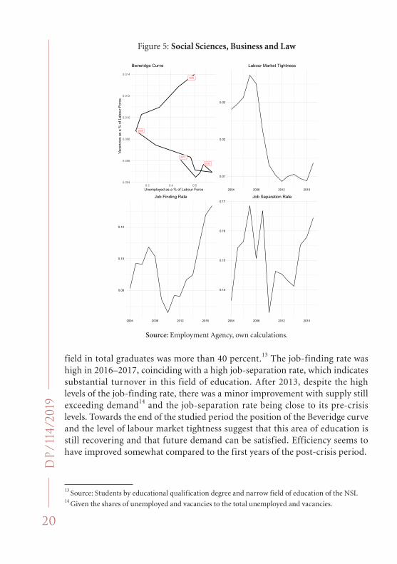
Over the pre-crisis period the Beveridge curve for this field of education (see Figure 5) was similar to that for the economy as a whole. With the onset of the global crisis the Beveridge curve took a downward course, indicating large-scale job destruction and rising unemployment. Labour market tightness was high in 2007–2008 and declined afterwards. However, the underlying factor was not lower labour supply. In the post-crisis period, demand (measured by the number of vacancies) was decreasing, while there was an increase in labour supply – in 2017 compared to 2008, the number of unemployed up to 39 years of age was nearly 140 percent higher and for those over the age of 40 there was a modest increase. The excess supply was due to the large flows of graduates for this fields of education: for the whole period the share of graduates in this

Figure 4: Humanities and Arts

comparatively low levels. This sector seems to be performing well toward theend of 2017 compared to the previous years, as there were still low levels oflabour market tightness and the job-finding rate stood at a historically highlevel, implying that efficiency in this field was relatively high. Also, theBeveridge curve began to move in a theoretically-consistent manner, withvacancies rising and unemployment declining.

Figure 4: Humanities and Arts

2004

2008

2013

2017

0.005

0.007

0.009

0.011


Vaca

ncie

s as

a %

of L

abou

r For

ce

Beveridge Curve

0.08

0.10

0.12

0.14

2004 2008 2012 2016

Job Finding Rate

0.04

0.05

0.06

0.07

0.08

0.09

2004 2008 2012 2016


0.16

0.18

0.20

0.22

2004 2008 2012 2016

Job Separation Rate


4.1.3. Specialists with education in “Social sciences, business and law”

Over the pre-crisis period the Beveridge curve for this field of education (seeFigure 5) was similar to that for the economy as a whole. With the onset of theglobal crisis the Beveridge curve took a downward course, indicating large-scalejob destruction and rising unemployment. Labour market tightness was high in2007 – 2008 and declined afterwards. However, the underlying factor was notlower labour supply. In the post-crisis period, demand (measured by the numberof vacancies) was decreasing, while there was an increase in labour supply – in 2017compared to 2008, the number of unemployed up to 39 years of age was nearly 140percent higher and for those over the age of 40 there was a modest increase. Theexcess supply was due to the large flows of graduates for this fields of education:

15


20

DP

/114

/201

9

field in total graduates was more than 40 percent.13 The job-finding rate was high in 2016–2017, coinciding with a high job-separation rate, which indicates substantial turnover in this field of education. After 2013, despite the high levels of the job-finding rate, there was a minor improvement with supply still exceeding demand14 and the job-separation rate being close to its pre-crisis levels. Towards the end of the studied period the position of the Beveridge curve and the level of labour market tightness suggest that this area of education is still recovering and that future demand can be satisfied. Efficiency seems to have improved somewhat compared to the first years of the post-crisis period.

13 Source: Students by educational qualification degree and narrow field of education of the NSI. 14 Given the shares of unemployed and vacancies to the total unemployed and vacancies.

Figure 5: Social Sciences, Business and Law

for the whole period the share of graduates in this field in total graduates wasmore than 40 percent13. The job-finding rate was high in 2016 – 2017, coincidingwith a high job-separation rate, which indicates substantial turnover in this fieldof education. After 2013, despite the high levels of the job-finding rate, there wasa minor improvement with supply still exceeding demand14 and the job-separationrate being close to its pre-crisis levels. Towards the end of the studied period theposition of the Beveridge curve and the level of labour market tightness suggestthat this area of education is still recovering and that future demand can besatisfied. Efficiency seems to have improved somewhat compared to the first yearsof the post-crisis period.

Figure 5: Social sciences, business and law

2004

2008

2013

2017

0.004

0.006

0.008

0.010

0.012

0.014

0.3 0.4 0.5Unemployed as a % of Labour Force

Vaca

ncie

s as

a %

of L

abou

r For

ce

Beveridge Curve

0.08

0.10

0.12

2004 2008 2012 2016

Job Finding Rate

0.01

0.02

0.03

2004 2008 2012 2016


0.14

0.15

0.16

0.17

2004 2008 2012 2016

Job Separation Rate


4.1.4. Specialists with education in “Education”

According to the Beveridge curve the rise of unemployment in this field ofeducation began in 2007 (see Figure 6), but due to the importance of the sector andits public funding, the curve moved inward relatively quickly in 2010. After that,

13Source: Students by educational qualification degree and narrow field of education of the NSI.14Given the shares of unemployed and vacancies to the total unemployed and vacancies.

16


21

DISC

USSIO

N PAPER

S

4.1.4. Specialists with education in “education”

According to the Beveridge curve the rise of unemployment in this field of education began in 2007 (see Figure 6), but due to the importance of the sector and its public funding, the curve moved inward relatively quickly in 2010. After that, job vacancies started to grow very fast without having a substantial impact on unemployment, most likely due to the limited labour supply. The main reason for the constrained supply seems to be the ageing of staff15 (over 50 percent of teachers are 50 years old or over) and the low number of new entrants in the system. After 2011, this field of education experienced high values of labour market tightness due both to higher labour demand and lower supply. According to the age structure of the unemployed, labour supply

15 Source: Teaching staff in general schools by age, NSI.

Figure 6: Education

job vacancies started to grow very fast without having a substantial impact onunemployment, most likely due to the limited labour supply. The main reason forthe constrained supply seems to be the ageing of staff15 (over 50 percent of teachersare 50 years old or over) and the low number of new entrants in the system. After2011, this field of education experienced high values of labour market tightness dueboth to higher labour demand and lower supply. According to the age structureof the unemployed, labour supply decreased on average by about 30 percent bothin the age group up to 39 and for those over 40 years of age. Despite the earliershift of the Beveridge curve and the fast increase of vacancies, the job-finding ratereached its pre-crisis levels only recently. The job-separation rate moved in linewith the Beveridge curve, with a spike in 2007. Toward the end of the periodanalysed this indicator stood at intermediate levels. The implications for labourmarket efficiency are not definitive, as the Beveridge curve moved inward andupward, indicating rising efficiency, while at the same time there was insufficientsupply according to the labour market tightness indicator.

Figure 6: Education

2004

2008

2013

2017

0.0075

0.0100

0.0125

0.0150

0.0175

0.075 0.100 0.125 0.150 0.175Unemployed as a % of Labour Force

Vaca

ncie

s as

a %

of L

abou

r For

ce

Beveridge Curve

0.10

0.12

0.14

0.16

2004 2008 2012 2016

Job Finding Rate

0.10

0.15

0.20

2004 2008 2012 2016


0.16

0.18

0.20

0.22

2004 2008 2012 2016

Job Separation Rate


15Source: Teaching staff in general schools by age, NSI.

17


22

DP

/114

/201

9decreased on average by about 30 percent both in the age group up to 39 and for those over 40 years of age. Despite the earlier shift of the Beveridge curve and the fast increase of vacancies, the job-finding rate reached its pre-crisis levels only recently. The job-separation rate moved in line with the Beveridge curve, with a spike in 2007. Toward the end of the period analysed this indicator stood at intermediate levels. The implications for labour market efficiency are not definitive, as the Beveridge curve moved inward and upward, indicating rising efficiency, while at the same time there was insufficient supply according to the labour market tightness indicator.

4.1.5. Specialists with education in “Health and welfare”

Over the period 2004–2007, the Beveridge curve in this field of education (see Figure 7) moved down and to the left, indicating a gradual filling of vacancies and a drop in unemployment. After 2008 there was a large fluctuation in

Figure 7: Health and WelfareFigure 7: Health and welfare

2004

2008

2013

2017

0.0030

0.0035

0.0040

0.0045


Vaca

ncie

s as

a %

of L

abou

r For

ce

Beveridge Curve

0.08

0.10

0.12

2004 2008 2012 2016

Job Finding Rate

0.05

0.06

0.07

0.08

0.09

2004 2008 2012 2016


0.14

0.15

0.16

2004 2008 2012 2016

Job Separation Rate


4.1.6. Specialists with education in “Science”

As evident from the Beveridge curve, unemployment started to increase in 2007(see Figure 8) and moved inward in 2012. The labour market tightness indicatorsuggests that there was enough labour supply in post-crisis period (mainly due tothe increase in the number of unemployed up to the age of 39), with the indicatorposting a rise only recently. The job-finding rate increased in upturns similarlyto other fields of education, and stood at a high level in 2017. The peak of thejob-separation rate in 2007 is in line with the dynamics of the Beveridge curve.Toward the end of the sample the job-separation rate stood at comparatively lowlevels. Given the higher unemployment rate and the lower level of vacancies, overthe post-crisis period labour market efficiency appears lower than in the pre-crisisperiod.

19


23

DISC

USSIO

N PAPER

Svacancies and a slight increase in unemployment. The much lower increase in unemployment compared to other fields of education even over the global crisis period reveals the inelastic demand for healthcare professionals. Starting in 2004 the labour market tightness in this field was on the rise, indicating insufficient labour supply, with a slight decrease between 2010 and 2014. According to the age structure of unemployed, in 2017 compared to 2008 the number of unemployed up to the age of 39 increased by 44 percent, while those over 40 years of age decreased by 25 percent. Despite the decrease, the number of persons in the second group was higher.

By 2017 job-finding and job-separation rates had reached historically high levels, suggesting high turnover in this field of education. Most likely this is due to the growing share of private healthcare spending.16 Additionally, it is likely that the establishment of a large number of private hospitals has contributed to the expanded pool of job opportunities for the healthcare professionals.

The relatively larger discrepancy between the shares of unemployed and vacancies as a percent of the total in the “Education” and “Health and welfare” fields compared to the other specializations may be due to the fact that these sectors have large public sector participation. The respective institutions (schools and hospitals) are obliged to post vacancies at the Employment Agency, while in the private sector this is optional and the decision to do so is usually related to applying for various subsidized employment schemes.

4.1.6. Specialists with education in “Science”

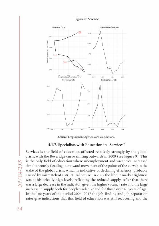
As evident from the Beveridge curve, unemployment started to increase in 2007 (see Figure 8) and moved inward in 2012. The labour market tightness indicator suggests that there was enough labour supply in post-crisis period (mainly due to the increase in the number of unemployed up to the age of 39), with the indicator posting a rise only recently. The job-finding rate increased in upturns similarly to other fields of education, and stood at a high level in 2017. The peak of the job-separation rate in 2007 is in line with the dynamics of the Beveridge curve. Toward the end of the sample the job-separation rate stood at comparatively low levels. Given the higher unemployment rate and the lower level of vacancies, over the post-crisis period labour market efficiency appears lower than in the pre-crisis period.

16 Source: System of Health Accounts, NSI.

24

DP

/114

/201

9Figure 8: ScienceFigure 8: Science

2004

2008

2013

2017

0.002

0.003

0.004

0.005


Vaca

ncie

s as

a %

of L

abou

r For

ce

Beveridge Curve

0.08

0.10

0.12

0.14

2004 2008 2012 2016

Job Finding Rate

0.025

0.050

0.075

0.100

0.125

2004 2008 2012 2016


0.15

0.18

0.21

0.24

2004 2008 2012 2016

Job Separation Rate


4.1.7. Specialists with education in “Services”

Services is the field of education affected relatively strongly by the global crisis,with the Beveridge curve shifting outwards in 2009 (see Figure 9). This is the onlyfield of education where unemployment and vacancies increased simultaneously(leading to outward movement of the points of the curve) in the wake of the globalcrisis, which is indicative of declining efficiency, probably caused by mismatch ofa structural nature. In 2007 the labour market tightness was at historically highlevels, reflecting the reduced supply. After that there was a large decrease in theindicator, given the higher vacancy rate and the large increase in supply bothfor people under 39 and for those over 40 years of age. In the last years ofthe period 2004 – 2017 the job-finding and job-separation rates give indicationsthat this field of education was still recovering and the unemployment rate wassubstantially above its 2008 levels. Given the level of vacancies, this points to anexisting mismatch and low efficiency.

20


4.1.7. Specialists with education in “Services”

Services is the field of education affected relatively strongly by the global crisis, with the Beveridge curve shifting outwards in 2009 (see Figure 9). This is the only field of education where unemployment and vacancies increased simultaneously (leading to outward movement of the points of the curve) in the wake of the global crisis, which is indicative of declining efficiency, probably caused by mismatch of a structural nature. In 2007 the labour market tightness was at historically high levels, reflecting the reduced supply. After that there was a large decrease in the indicator, given the higher vacancy rate and the large increase in supply both for people under 39 and for those over 40 years of age. In the last years of the period 2004–2017 the job-finding and job-separation rates give indications that this field of education was still recovering and the

25

DISC

USSIO

N PAPER

Sunemployment rate was substantially above its 2008 levels. Given the level of vacancies, this points to an

Figure 9: ServicesFigure 9: Services

2004

2008

20132017

0.015

0.020


Vaca

ncie

s as

a %

of L

abou

r For

ceBeveridge Curve

0.07

0.09

0.11

0.13

0.15

2004 2008 2012 2016

Job Finding Rate

0.05

0.10

0.15

0.20

0.25

2004 2008 2012 2016


0.175

0.200

0.225

2004 2008 2012 2016

Job Separation Rate


4.1.8. Specialists with education in “Engineering, manufacturing andconstruction”

Unemployed and vacancies for this educational field declined simultaneouslyover almost the entire period, with the Beveridge curve sloping upwards (seeFigure 10). The global crisis period was an exception to this pattern, and therewas another temporary outward shift in 2012, probably caused by thesovereign-debt crisis in Europe. With the onset of global crisis and theconcomitant contraction in construction activity, the demand for constructionspecialists dropped, which is a possible explanation for the declining vacancyrate in the post-crisis period. Tightness experienced a big drop in the post-crisisperiod and stood at relatively low levels toward the end of 2017. The dynamicsof the job-finding rate after 2015 imply a higher probability of finding a job forunemployed persons with such specialization, while the job-separation rate stoodat moderate levels. As far as the age structure of the unemployed is concerned,in the post-crisis period, the unemployed up to the age of 39 were increasing,and those over the age of 40 were on the decrease. The lower levels of vacanciesindicate depressed labour demand. Despite that, the unemployment rate and

21


4.1.8. Specialists with education in “engineering, manufacturing and construction”

Unemployed and vacancies for this educational field declined simultaneously over almost the entire period, with the Beveridge curve sloping upwards (see Figure 10). The global crisis period was an exception to this pattern, and there was another temporary outward shift in 2012, probably caused by the sovereign-debt crisis in Europe. With the onset of global crisis and the concomitant contraction in construction activity, the demand for construction specialists dropped, which is a possible explanation for the declining vacancy rate in the post-crisis period. Tightness experienced a big drop in the post-crisis period and stood at relatively low levels toward the end of 2017. The dynamics of the job-finding rate after

26

DP

/114

/201

9

2015 imply a higher probability of finding a job for unemployed persons with such specialization, while the job-separation rate stood at moderate levels. As far as the age structure of the unemployed is concerned, in the post-crisis period, the unemployed up to the age of 39 were increasing, and those over the age of 40 were on the decrease. The lower levels of vacancies indicate depressed labour demand. Despite that, the unemployment rate and labour market tightness were low, indicating high efficiency in this sector.

4.1.9. persons without educational Qualification Having primary education

The group of people with primary or lower education occupies the largest share among job-seekers registered at the Employment Agency. One possible explanation is that these people are experiencing greater difficulty finding a job and need an intermediary in this effort. There was no substantial rise in

Figure 10: Engineering, Manufacturing and Construction

labour market tightness were low, indicating high efficiency in this sector.

Figure 10: Engineering, manufacturing and construction

2004

2008

2013

2017

0.01

0.02

0.03


Vaca

ncie

s as

a %

of L

abou

r For

ce

Beveridge Curve

0.06

0.08

0.10

0.12

2004 2008 2012 2016

Job Finding Rate

0.01

0.02

0.03

0.04

2004 2008 2012 2016


0.13

0.14

0.15

0.16

2004 2008 2012 2016

Job Separation Rate


4.1.9. Persons without educational qualification having primary education

The group of people with primary or lower education occupies the largestshare among job-seekers registered at the Employment Agency. One possibleexplanation is that these people are experiencing greater difficulty finding a joband need an intermediary in this effort. There was no substantial rise inunemployment for this group after 2008 according to the Beveridge curve (seeFigure 11). The reasons for this could be the general decline in the number ofpersons with basic and lower education, and their transition to higherqualification groups, as well as the bigger propensity of these individuals to leavethe workforce. Age data confirms the above statement, with the unemployed upto 39 years of age declining by 24 percent in 2017 compared to 2008. Between2010 and 2015 vacancies rose without any response in unemployment, indicatingdeclining efficiency in this period. Toward the end of the 2017 the labour markettightness indicator for this field of education stood at its highest values, whichcan be interpreted as evidence of emerging labour shortages, which may haveforced entrepreneurs to recruit less educated workers. The job-finding rate was

22


27

DISC

USSIO

N PAPER

Sunemployment for this group after 2008 according to the Beveridge curve (see Figure 11). The reasons for this could be the general decline in the number of persons with basic and lower education, and their transition to higher qualification groups, as well as the bigger propensity of these individuals to leave the workforce. Age data confirms the above statement, with the unemployed up to 39 years of age declining by 24 percent in 2017 compared to 2008. Between 2010 and 2015 vacancies rose without any response in unemployment, indicating declining efficiency in this period. Toward the end of the 2017 the labour market tightness indicator for this field of education stood at its highest values, which can be interpreted as evidence of emerging labour shortages, which may have forced entrepreneurs to recruit less educated workers. The job-finding rate was consistent with the tightness indicator and started to recover after 2015. Firms laid off workers with primary education more intensively only in 2009 and toward the end of the period the indicator

Figure 11: Primary Education

consistent with the tightness indicator and started to recover after 2015. Firmslaid off workers with primary education more intensively only in 2009 and towardthe end of the period the indicator was at low levels. After 2015, unemploymentis declining with job-finding rate going up, which we interpret as rising efficiency.

Figure 11: Primary Education

2004

2008

2013

2017

0.16

0.20

0.24

3 4 5 6 7Unemployed as a % of Labour Force

Vaca

ncie

s as

a %

of L

abou

r For

ce

Beveridge Curve

0.03

0.04

0.05

2004 2008 2012 2016

Job Finding Rate

0.02

0.04

0.06

0.08

2004 2008 2012 2016


0.07

0.08

0.09

0.10

0.11

2004 2008 2012 2016

Job Separation Rate


4.1.10. Persons without educational qualification having secondaryeducation

This group was strongly affected by the global crisis. The Beveridge curveshifted its movement in 2009 and moved downward until 2012 (see Figure 12).With the increase of demand in the post-crisis period, labour market tightnessbegan to increase, reaching the highest values in 2016 – 2017. The recovery ofefficiency started in 2012 with an increase in the job-finding rate and the numberof vacancies, yet labour demand increased more than supply and theunemployment-vacancy points on the Beveridge curve began moving inward andup, i.e. there was a slight decrease in unemployment accompanied by a sharpincrease in vacancies. The job-separation rate reached its peak in 2007,accompanied by another one in 2009. Similar levels were recorded toward theend of the period under investigation. In 2017 compared to 2007 the number of

23


28

DP

/114

/201

9was at low levels. After 2015, unemployment is declining with job-finding rate going up, which we interpret as rising efficiency.

4.1.10. persons without educational Qualification Having Secondary education

This group was strongly affected by the global crisis. The Beveridge curve shifted its movement in 2009 and moved downward until 2012 (see Figure 12). With the increase of demand in the post-crisis period, labour market tightness began to increase, reaching the highest values in 2016–2017. The recovery of efficiency started in 2012 with an increase in the job-finding rate and the number of vacancies, yet labour demand increased more than supply and the unemployment-vacancy points on the Beveridge curve began moving inward and up, i.e. there was a slight decrease in unemployment accompanied by a

Figure 12: Secondary Education

unemployed persons with secondary education increased by 24 percent, probablyas a result of a general increase in the educational level of the population and, inparticular, of those with primary education. The position of the Beveridge curvewith respect to the axes suggests that in this group the labour market hasbecome less efficient, with a higher unemployment rate despite the largerdemand.

Figure 12: Secondary Education

2004

2008

2013

2017

0.08

0.12

0.16

0.20


Vaca

ncie

s as

a %

of L

abou

r For

ce

Beveridge Curve

0.06

0.08

0.10

0.12

2004 2008 2012 2016

Job Finding Rate

0.1

0.2

0.3

2004 2008 2012 2016


0.14

0.15

0.16

0.17

0.18

2004 2008 2012 2016

Job Separation Rate


4.1.11. Persons without educational qualification having workers’professions

Persons with workers professions constitute the second largest subgroup in theunemployment pool after primary education. The Beveridge curve moveddownward in pre-crisis period for this educational field, with 2009 being theturning point (see Figure 13). A process of recovery started in 2015 with theBeveridge curve reversing direction, yet a rise in vacancies was only observed in2017. Labour market tightness was relatively high in the pre-crisis period butwith falling demand after 2009 it rapidly decreased. The dynamics of thejob-finding rate were similar to those for the primary education field, with theexception that it reached its maximum in 2017. The job-separation rate peaked

24


29

DISC

USSIO

N PAPER

Ssharp increase in vacancies. The job-separation rate reached its peak in 2007, accompanied by another one in 2009. Similar levels were recorded toward the end of the period under investigation. In 2017 compared to 2007 the number of unemployed persons with secondary education increased by 24 percent, probably as a result of a general increase in the educational level of the population and, in particular, of those with primary education. The position of the Beveridge curve with respect to the axes suggests that in this group the labour market has become less efficient, with a higher unemployment rate despite the larger demand.

4.1.11. persons without educational Qualification Having workers’ professions

Persons with workers professions constitute the second largest subgroup in the unemployment pool after primary education. The Beveridge curve moved downward in pre-crisis period for this educational field, with 2009 being the turning point (see Figure 13). A process of recovery started in 2015 with the Beveridge curve reversing direction, yet a rise in vacancies was only observed in 2017. Labour market tightness was relatively high in the pre-crisis period but with falling demand after 2009 it rapidly decreased. The dynamics of the job-finding rate were similar to those for the primary education field, with the exception that it reached its maximum in 2017. The job-separation rate peaked in 2009, but stood at relatively low levels in the post-crisis period. In 2017, compared to 2008, there was an increase in the number of unemployed over the age of 40, while those up to the age of 39 remained almost unchanged, which can be interpreted as evidence of ageing in this group. Labour market efficiency in 2017 appears higher than pre-crisis period, reflecting almost the same unemployment rate as in 2007 and lower vacancy rate.

As a recapitulatory comment on the descriptive analysis by fields of education, the global financial crisis affected the different sectors across the board, but specific factors also had an impact. Labour market tightness peaked around 2008 for almost all fields of education, while post-crisis developments were more diverse and additional indicators suggest some heterogeneity of labour market outcomes across educational fields. During the 2015–2017 period there was declining efficiency in some fields of education, despite the increase in economic activity.

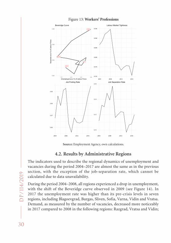
30

DP

/114

/201

9

4.2. results by administrative regionsThe indicators used to describe the regional dynamics of unemployment and vacancies during the period 2004–2017 are almost the same as in the previous section, with the exception of the job-separation rate, which cannot be calculated due to data unavailability.

During the period 2004–2008, all regions experienced a drop in unemployment, with the shift of the Beveridge curve observed in 2009 (see Figure 14). In 2017 the unemployment rate was higher than its pre-crisis levels in seven regions, including Blagoevgrad, Burgas, Sliven, Sofia, Varna, Vidin and Vratsa. Demand, as measured by the number of vacancies, decreased more noticeably in 2017 compared to 2008 in the following regions: Razgrad, Vratsa and Vidin;

Figure 13: Workers’ Professions

in 2009, but stood at relatively low levels in the post-crisis period. In 2017,compared to 2008, there was an increase in the number of unemployed over theage of 40, while those up to the age of 39 remained almost unchanged, which canbe interpreted as evidence of ageing in this group. Labour market efficiency in2017 appears higher than pre-crisis period, reflecting almost the sameunemployment rate as in 2007 and lower vacancy rate.

Figure 13: Workers’ Professions

2004

2008

2013

2017

0.02

0.04

0.06

0.08


Vaca

ncie

s as

a %

of L

abou

r For

ce

Beveridge Curve

0.06

0.07

0.08

0.09

2004 2008 2012 2016

Job Finding Rate

0.010

0.015

0.020

0.025

0.030

0.035

2004 2008 2012 2016


0.10

0.12

0.14

0.16

2004 2008 2012 2016

Job Separation Rate


As a recapitulatory comment on the descriptive analysis by fields of education,the global financial crisis affected the different sectors across the board, but specificfactors also had an impact. Labour market tightness peaked around 2008 foralmost all fields of education, while post-crisis developments were more diverseand additional indicators suggest some heterogeneity of labour market outcomesacross educational fields. During the 2015 – 2017 period there was decliningefficiency in some fields of education, despite the increase in economic activity.

4.2. Results by administrative regions

The indicators used to describe the regional dynamics of unemployment andvacancies during the period 2004 – 2017 are almost the same as in the previous

25


31

DISC

USSIO

N PAPER

Sin the latter two regions, unemployment was higher compared to 2008, which likely reflects labour demand problems in these regions.

Labour market tightness was rising during the 2004–2007 and 2013–2017 periods for almost all regions (see Figure 15). Administrative regions that did not reach the 2007–2008 levels of tightness by 2017 are located mostly in northern parts of the country (more noticeably in north-east and north-west), with the exception of Pernik, Sliven and Sofia, where tightness is also low. Labour market tightness is the lowest in the regions with the highest unemployment rates in the north-west and north-east part of the country.

The job-finding rate typically follows the dynamics of labour market tightness and this is the case for almost all regions (see Figure 16). In 2017 the job-finding rate recorded the maximum value for the period analysed in all regions of the country excluding Montana, Rouse, Shumen, Sofia, Vidin and Vratsa. This is consistent with the outcome for the tightness indicator, except for Rouse, where tightness was high in this period. Measured by the job-finding rate, the recovery started at the earliest in 2012 for the following regions: Gabrovo, Kyustendil, Plovdiv, Razgrad, Sofia, Sofia District, Stara Zagora, Targovishte, Varna and Veliko Tarnovo. In 2013, the job-finding rate in the regions of Burgas, Dobrich, Kardzhali, Lovech, Pazardzhik, Pernik, Rousse, Shumen, Silistra, Sliven, Smolyan and Yambol also responded, and in 2014 Haskovo and Pleven followed suit. The other four regions – Blagoevgrad, Montana, Vidin and Vratsa – underwent a rise and a sharp fall in the indicator over the period 2012–2014, probably linked to more extensive temporary employment schemes in these regions.

The implications of these facts for labour market efficiency are mixed, since regions with both higher levels of unemployment and job vacancies are expected to have, in principle, lower labour market efficiency in comparison to the pre-crisis period. Yet, for the big regional centres (Sofia, Burgas, Varna) this higher unemployment rate is due to the increased supply through the whole period, a direct consequence of substantial internal migration. For other regions (Vidin, Vratsa), where supply shrank, the higher level of unemployment is probably entrenched due to structural factors and may require specific policy actions in order to be resolved.

32

DP

/114

/201

9Figure 14: Beveridge Curve – Unemployed and Vacancies

as a Percent of Labour Force by RegionsFigure 14: Beveridge curve – unemployed and vacancies as a percent of labour

force by regions

2004

2008

20132017

2004

2008

20132017

2004

2008

2013

2017

2004

2008

2013

2017

2004

2008 2013

2017

2004

2008

20132017

2004

2008

20132017

2004

20082013

2017

2004

2008

2013

2017

2004

20082013

2017

2004

20082013

2017

2004

2008

20132017

2004

2008

20132017

2004

2008

2013

2017

2004

2008 2013

2017

2004

2008

20132017

2004

2008

20132017

2004

20082013

2017

2004

2008

20132017

2004

2008

20132017

2004

2008

2013

2017

2004

2008 2013

2017

2004

2008

20132017

2004

2008

2013

2017

2004

2008 2013

2017

2004

2008

2013

2017

2004

2008 2013

2017

2004

2008 2013

2017

Veliko Tarnovo Vidin Vratsa Yambol

Sofia District Stara Zagora Targovishte Varna

Silistra Sliven Smolyan Sofia

Plovdiv Razgrad Rousse Shumen

Montana Pazardjik Pernik Pleven

Haskovo Kardjali Kyustendil Lovetch

Blagoevgrad Burgas Dobrich Gabrovo

0.2 0.3 0.4 0.5 0.6 0.20 0.25 0.30 0.35 0.300.350.400.450.500.55 0.2 0.3

0.25 0.30 0.35 0.40 0.45 0.3 0.4 0.5 0.6 0.2 0.3 0.4 0.5 0.3 0.4 0.5 0.6

0.20 0.25 0.30 0.35 0.40 0.3 0.4 0.5 0.20 0.25 0.30 0.35 0.40 0.2 0.3 0.4 0.5 0.6 0.7

0.6 0.8 1.0 0.2 0.3 0.4 0.2 0.3 0.4 0.5 0.3 0.4 0.5

0.3 0.4 0.5 0.4 0.5 0.6 0.7 0.10 0.15 0.20 0.4 0.5 0.6 0.7

0.3 0.4 0.5 0.20 0.25 0.30 0.35 0.15 0.18 0.21 0.24 0.20 0.25 0.30

0.4 0.5 0.6 0.2 0.3 0.4 0.5 0.2 0.3 0.4 0.5 0.08 0.10 0.12 0.140.006

0.008

0.010

0.010

0.015

0.020

0.0150.0200.0250.0300.0350.040

0.015

0.020

0.025

0.030

0.04

0.05

0.06

0.07

0.02

0.03

0.04

0.05

0.010

0.015

0.020

0.010

0.015

0.020

0.025

0.030

0.012

0.016

0.020

0.0060.0080.0100.0120.014

0.02

0.03

0.016

0.020

0.024

0.028

0.005

0.010

0.015

0.020

0.025

0.01

0.02

0.03

0.010.020.030.040.05

0.009

0.012

0.015

0.0200.0250.0300.0350.040

0.0100.0150.0200.0250.030

0.012

0.016

0.020

0.0200.0250.0300.0350.040

0.010

0.015

0.020

0.025

0.024

0.028

0.032

0.036

0.010

0.015

0.020

0.025

0.0150.0200.0250.0300.035

0.03

0.04

0.05

0.06

0.010

0.015

0.020

0.02

0.03

0.04

0.02

0.03

Unemployed as a % of Labour Force

Vaca

ncie

s as

a %

of L

abou

r For

ce


27


33

DISC

USSIO

N PAPER

SFigure 15: Labour Market Tightness –

Ratio of Vacancies to Unemployed by RegionsFigure 15: Labour market tightness – ratio of vacancies to unemployed by regions








2004 2008 2012 2016 2004 2008 2012 2016 2004 2008 2012 2016 2004 2008 2012 2016

0.050

0.075

0.100

0.125

0.03

0.04

0.05

0.06

0.07

0.04

0.05

0.06

0.07

0.0350.0400.0450.0500.0550.0600.065

0.10

0.15

0.20

0.25

0.06

0.08

0.10

0.12

0.03

0.04

0.05

0.06

0.07

0.050

0.075

0.100

0.125

0.04

0.06

0.08

0.030.040.050.060.070.08

0.05

0.06

0.07

0.08

0.09

0.05

0.06

0.07

0.08

0.09

0.02

0.03

0.04

0.05

0.030.040.050.060.070.08

0.05

0.10

0.15

0.04

0.05

0.06

0.04

0.05

0.06

0.07

0.03

0.04

0.05

0.06

0.03

0.04

0.05

0.04

0.06

0.08

0.10

0.04

0.06

0.08

0.10

0.04

0.05

0.06

0.07

0.08

0.03

0.04

0.05

0.06

0.04

0.06

0.08

0.050

0.075

0.100

0.03

0.04

0.05

0.06

0.07

0.05

0.06

0.07

0.08

0.09

0.04

0.06

0.08

0.10


28


34

DP

/114

/201

9Figure 16: Job Finding Rate – Ratio of Job Starts to Unemployed

(End of Period) by RegionsFigure 16: Job finding rate – ratio of job starts to unemployed (end of period) byregions








2004 2008 2012 2016 2004 2008 2012 2016 2004 2008 2012 2016 2004 2008 2012 2016

0.05

0.07

0.09

0.11

0.13

0.04

0.05

0.06

0.07

0.08

0.04

0.05

0.06

0.07

0.04

0.05

0.06

0.07

0.09

0.12

0.15

0.18

0.07

0.09

0.11

0.04

0.05

0.06

0.07

0.08

0.06

0.08

0.10

0.12

0.06

0.08

0.10

0.06

0.07

0.08

0.09

0.10

0.05

0.06

0.07

0.08

0.09

0.06

0.07

0.08

0.09

0.03

0.04

0.05

0.06

0.04

0.05

0.06

0.07

0.08

0.09

0.06

0.08

0.10

0.12

0.03

0.04

0.05

0.06

0.04

0.05

0.06

0.035

0.040

0.045

0.050

0.055

0.060

0.03

0.04

0.05

0.06

0.06

0.08

0.10

0.04

0.05

0.06

0.07

0.08

0.09

0.05

0.06

0.07

0.08

0.04

0.05

0.06

0.07

0.04

0.05

0.06

0.07

0.08

0.04

0.05

0.06

0.07

0.08

0.04

0.05

0.06

0.06

0.07

0.08

0.09

0.06

0.08

0.10

0.12


29


35

DISC

USSIO

N PAPER

S5. econometric results

5.1. methodology

5.1.1. General Notes

Our approach to assessing the degree of labour market efficiency for the Bulgarian economy exploits the matching function as given by equation (1) and estimates it in a panel model framework. The matching function framework is a prominent approach to modelling labour market efficiency and constitutes a natural first step in studying these issues. Moreover, the available data is conducive to the application of this approach to the analysis of the Bulgarian labour market. The particular implementation works with a modification of equation (1) that was proposed by Barnichon and Figura (2011). The modification seeks to relax the assumption that transitions between employment and unemployment occur only within regions or fields of education that is implicit in the standard matching function approach. In cases where granular data on transitions between various forms of employment are unavailable, Barnichon and Figura (2011) suggest to use the specification

5. Econometric results

5.1. Methodology

5.1.1. General notes

Our approach to assessing the degree of labour market efficiency for theBulgarian economy exploits the matching function as given by equation (1) andestimates it in a panel model framework. The matching function framework is aprominent approach to modelling labour market efficiency and constitutes anatural first step in studying these issues. Moreover, the available data isconducive to the application of this approach to the analysis of the Bulgarianlabour market. The particular implementation works with a modification ofequation (1) that was proposed by Barnichon and Figura (2011). Themodification seeks to relax the assumption that transitions between employmentand unemployment occur only within regions or fields of education that isimplicit in the standard matching function approach. In cases where granulardata on transitions between various forms of employment are unavailable,Barnichon and Figura (2011) suggest to use the specification

jfit = miθζitθ

1−ζt , (4)

where the subscript i denotes the units (regions or fields of education) and theoverall tightness θt serves as a proxy for transitions between sectors (i.e. findingemployment in a different field of education or region). The termmi can be treatedas a slightly generalised version of the intercept ET (lnm0t) in equation (3).Taking logs in equation (4), we can estimate it and use the residuals as a measure

of the sectoral deviations of matching efficiency around the respective long-runlevel. Going along this route effectively means that one focuses on the dynamicsof efficiency for a specified sector without attempting comparisons of the level ofefficiency across units (fields of education or regions in our case). As a consequence,while we report the estimated intercepts for the random effects models that arepresented below, we do not attach any special significance to these values and treatthem merely as inputs for the computation of the matching efficiency deviationsfrom the long-run mean. However, in the discussion of the econometric analysisresults we still use the term “efficiency” as a shortcut in order to avoid cumbersomereferences to the deviations of efficiency from its long-run level.The above approach should not be treated as a strictly econometric one, since

it entails working with a fixed theoretical structure and therefore loses some ofthe flexibility associated with a purely statistical approach to estimating theassociation between the job-finding rate and tightness indicators. At the sametime, it is necessary to test and modify accordingly those aspects of theestimation procedure that are not affected by the constraints of the chosentheoretical framework. We outline the main steps of this approach in thefollowing paragraphs. The results reported relate to equation (4), transformed inlogarithmic form. Note that, since the coefficients for sectoral tightness andoverall tightness are constrained to sum to one, the coefficient for overalltightness can be treated as derivable from that for sectoral tightness, Thus, wecan equivalently estimate a transformed version of the logged equation (4), forwhich ζ is the coefficient multiplying the difference of the logarithms of sectoral

30

, (4)

where the subscript i denotes the units (regions or fields of education) and the overall tightness qt serves as a proxy for transitions between sectors (i.e. finding employment in a different field of education or region). The term mi

can be treated as a slightly generalised version of the intercept





Ut+1 = Ut −Mt + (1− Ut)λt,



At =

[λt

Ut

− λt

](Ut

Vt

)1−α





7

in equation (3).

Taking logs in equation (4), we can estimate it and use the residuals as a measure of the sectoral deviations of matching efficiency around the respective long-run level. Going along this route effectively means that one focuses on the dynamics of efficiency for a specified sector without attempting comparisons of the level of efficiency across units (fields of education or regions in our case). As a consequence, while we report the estimated intercepts for the random effects models that are presented below, we do not attach any special significance to these values and treat them merely as inputs for the computation of the matching efficiency deviations from the long-run mean. However, in the discussion of the econometric analysis results we still use the term “efficiency” as a shortcut in order to avoid cumbersome references to the deviations of efficiency from its long-run level.

The above approach should not be treated as a strictly econometric one, since it entails working with a fixed theoretical structure and therefore loses some

36

DP

/114

/201

9of the flexibility associated with a purely statistical approach to estimating the association between the job-finding rate and tightness indicators. At the same time, it is necessary to test and modify accordingly those aspects of the estimation procedure that are not affected by the constraints of the chosen theoretical framework. We outline the main steps of this approach in the following paragraphs. The results reported relate to equation (4), transformed in logarithmic form. Note that, since the coefficients for sectoral tightness and overall tightness are constrained to sum to one, the coefficient for overall tightness can be treated as derivable from that for sectoral tightness, Thus, we can equivalently estimate a transformed version of the logged equation (4), for which z is the coefficient multiplying the difference of the logarithms of sectoral and overall tightness. As this approach constitutes a technical detail of the implementation and does not have substantive implications, we retain the use of the terms “sectoral tightness” and “regional tightness” in all tables reporting the estimation results below.

Since our main approach follows the theoretical structure prescribed by (4) and therefore enforces a constraint of the constant returns to scale type, it is legitimate to ask to what extent the latter constraint impacts the results. To address this question, the appendix presents the results from testing and estimating an unconstrained version of equation (4), i.e.

and overall tightness. As this approach constitutes a technical detail of theimplementation and does not have substantive implications, we retain the use ofthe terms “sectoral tightness” and “regional tightness” in all tables reporting theestimation results below.Since our main approach follows the theoretical structure prescribed by (4)

and therefore enforces a constraint of the constant returns to scale type, it islegitimate to ask to what extent the latter constraint impacts the results. Toaddress this question, the appendix presents the results from testing andestimating an unconstrained version of equation (4), i.e. jfit = miθ

ζ1it θ

ζ2t . Overall,

these results provide some evidence in favour of a decreasing-returns-to-scalespecification of the matching function. The different methods (including theconstrained versions of the model with either individual or time effects) alsoexhibit sensitivity of the sectoral tightness estimates with respect to thespecification and the chosen estimation routine. Additionally, testing forautocorrelation in the residuals gives positive indications of autocorrelation,which can be anticipated in view of the monthly frequency of the sample data.Taken together, these findings suggest that in future research considerationneeds to be given to the tradeoff between adherence to an established theoreticalframework versus exploiting a more data-driven but potentially less interpretableapproach. The present work follows the first route, which can be interpreted asimposing a theory prior on the econometric analysis.Our current approach takes the following steps to check the validity of the

procedures employed and determine the details of the estimation method. First,we conduct a poolability test in order to establish whether using a panel estimationmethod holds any advantages over pooling the data and estimating an ordinaryregression. Second, we test the appropriateness of including individual, time ortwo-way effects. Third, we run a Hausman test to determine whether to use afixed-effect or random-effect estimation procedure. Following that, we estimatethe respective equations and extract the residuals to be used as a measure ofefficiency variation.The above steps were applied separately to the data by fields of education and by

regions. The next subsection reports the details for the two tracks of the analysis.

5.1.2. Testing and estimation results for the fields of education breakdown

The results of the poolability test for the fields of education data are presentedin Table 3 in the appendix. Based on the test we can reject the null hypothesisof identical coefficients at the 0.1% level, which implies that we can proceed withestimation in a panel data framework.Tables 4, 5 and 6 in the appendix report the results of testing for individual,

time and two-way effects. For our model there is evidence supporting the threetypes of effects. We can thus take the two-way effects as the main specification,with individual and time effects used for comparison purposes.To determine whether to estimate a fixed-effect or a random-effect model, we

run a Hausman test. The results, presented in Table 7 in the appendix, indicatethat random effects estimation is the appropriate route to take.Based on the above testing framework, we estimate a two-way effect model

based on equation (4). The results are provided in Table 1.

31

. Overall, these results provide some evidence in favour of a decreasing-returns-to-scale specification of the matching function. The different methods (including the constrained versions of the model with either individual or time effects) also exhibit sensitivity of the sectoral tightness estimates with respect to the specification and the chosen estimation routine. Additionally, testing for autocorrelation in the residuals gives positive indications of autocorrelation, which can be anticipated in view of the monthly frequency of the sample data. Taken together, these findings suggest that in future research consideration needs to be given to the tradeoff between adherence to an established theoretical framework versus exploiting a more data-driven but potentially less interpretable approach. The present work follows the first route, which can be interpreted as imposing a theory prior on the econometric analysis.

Our current approach takes the following steps to check the validity of the procedures employed and determine the details of the estimation method. First, we conduct a poolability test in order to establish whether using a panel estimation method holds any advantages over pooling the data and estimating an ordinary regression. Second, we test the appropriateness of including individual, time or two-way effects. Third, we run a Hausman test to determine whether to use a fixed-effect or random-effect estimation procedure. Following

37

DISC

USSIO

N PAPER

Sthat, we estimate the respective equations and extract the residuals to be used as a measure of efficiency variation.

The above steps were applied separately to the data by fields of education and by regions. The next subsection reports the details for the two tracks of the analysis.

5.1.2. testing and estimation results for the fields of education Breakdown

The results of the poolability test for the fields of education data are presented in Table 3 in the appendix. Based on the test we can reject the null hypothesis of identical coefficients at the 0.1% level, which implies that we can proceed with estimation in a panel data framework.

Tables 4, 5 and 6 in the appendix report the results of testing for individual, time and two-way effects. For our model there is evidence supporting the three types of effects. We can thus take the two-way effects as the main specification, with individual and time effects used for comparison purposes.

To determine whether to estimate a fixed-effect or a random-effect model, we run a Hausman test. The results, presented in Table 7 in the appendix, indicate that random effects estimation is the appropriate route to take.

Based on the above testing framework, we estimate a two-way effect model based on equation (4). The results are provided in Table 1.

Table 1: Restricted Matching Function Regression, Fields of Education Data, Two-way Effects

Dependent variable:

Job-finding rate

Sectoral tightness 0.032∗∗∗

(0.005)

Constant −2.431∗∗∗

(0.097)

Observations 1,848R2 0.018Adjusted R2 0.018F Statistic 34.686∗∗∗ (df = 1; 1846)

Note: ∗p<0.1; ∗∗p<0.05; ∗∗∗p<0.01

Table 1: Restricted matching function regression, fields of education data, two-wayeffects

For comparison, in the appendix we present the results from estimating anindividual effects model in Table 8 and those for a time effects model in Table 9.

5.1.3. Testing and estimation results for the regional breakdown

In parallel to the approach employed for the fields of education breakdown, wepresent the results of the poolability test for the regional data in Table 10 in theappendix. The null hypothesis of identical coefficients can be rejected at the 0.1%level, therefore estimation in a panel data framework is legitimate.Tables 11, 12 and 13 in the appendix report the results of testing for individual,

time and two-way effects. Again, evidence supporting the three types of effects isfound, mirroring results for the fields of education case. Correspondingly, we takethe two-way effects as the main specification and report the individual and timeeffects cases for comparison.The results of the Hausman test are reported in Table 14 in the appendix. They

indicate that employing fixed effects estimation is appropriate.At the estimation step, we estimate the two-way effect model and report the

results in Table 2. This compares with the results from estimating an individualeffects model as shown in Table 15 and those for a time effects model, which areprovided in Table 16, both presented in the appendix.

5.2. Estimated changes in labour market matching efficiencyacross fields of education

The dynamics of labour market matching efficiency vary across fields ofeducation (see Figure 17). The most significant improvement in comparison tothe pre-2008 period was recorded in the following fields of education:“Agriculture”, “Social science, business and law” and “Engineering,

32

38

DP

/114

/201

9For comparison, in the appendix we present the results from estimating an individual effects model in Table 8 and those for a time effects model in Table 9.

5.1.3. testing and estimation results for the regional Breakdown

In parallel to the approach employed for the fields of education breakdown, we present the results of the poolability test for the regional data in Table 10 in the appendix. The null hypothesis of identical coefficients can be rejected at the 0.1% level, therefore estimation in a panel data framework is legitimate.

Tables 11, 12 and 13 in the appendix report the results of testing for individual, time and two-way effects. Again, evidence supporting the three types of effects is found, mirroring results for the fields of education case. Correspondingly, we take the two-way effects as the main specification and report the individual and time effects cases for comparison.

The results of the Hausman test are reported in Table 14 in the appendix. They indicate that employing fixed effects estimation is appropriate.

At the estimation step, we estimate the two-way effect model and report the results in Table 2. This compares with the results from estimating an individual effects model as shown in Table 15 and those for a time effects model, which are provided in Table 16, both presented in the appendix.

5.2. estimated changes in Labour market matching efficiency across fields of education

The dynamics of labour market matching efficiency vary across fields of education (see Figure 17). The most significant improvement in comparison to the pre-2008 period was recorded in the following fields of education: “Agriculture”, “Social science, business and law” and “Engineering, manufacturing and construction”. Conversely, other fields, such as “Science”, “Primary Education” and “Services”, experienced a decline in efficiency.

39

DISC

USSIO

N PAPER

SFigure 17: Labour Market Efficiency Dynamics by Field of EducationFigure 17: Labour market efficiency dynamics by field of education

Social sciences, business and law Workers` Professions

Science Secondary Education Services

Health and welfare Humanities and Arts Primary Education

Agricultural Education Engineering, manufacturing & construction

2005 2010 2015 2005 2010 2015

2005 2010 2015 2005 2010 2015 2005 2010 2015

2005 2010 2015 2005 2010 2015 2005 2010 2015

2005 2010 2015 2005 2010 2015 2005 2010 2015

−0.1

0.0

0.1

−0.2

−0.1

0.0

0.1

0.2

−0.2

0.0

0.2

0.4

−0.2

−0.1

0.0

0.1

−0.1

0.0

0.1

−0.10

−0.05

0.00

0.05

0.10

−0.10

−0.05

0.00

0.05

0.10

0.15

−0.2

−0.1

0.0

0.1

−0.10

−0.05

0.00

0.05

0.10

−0.1

0.0

0.1

−0.2

−0.1

0.0

0.1

Source: Own calculations.

The rising efficiency in “Agriculture” is related to both lower demand andlower supply of labour, which is a direct consequence of the sector-specific factorsdiscussed in Section 4. The increase in supply for “Social science, business andlaw” from 2000 onwards has matched the rising demand over past years. Theimproved efficiency in the field of education “Engineering, manufacturing andconstruction” is associated with a reduction in the large labour supply observedbefore 2008 and the higher job-finding rate after 2012.In the field of education “Science” the efficiency started to recover from 2013 up

to 2015. After 2015 the efficiency in this field declined again. This can be relatedto the rising demand for specialists with education in sectors such as computerscience and communications, and the relatively slow response of supply.

34


40

DP

/114

/201

9Table 2: Restricted Matching Function Regression,

Regional Data, Two-way Effects

Dependent variable:

Job-finding rate

Regional tightness 0.055∗∗∗

(0.004)

Observations 4,676R2 0.032Adjusted R2 −0.010F Statistic 147.172∗∗∗ (df = 1; 4481)

Note: ∗p<0.1; ∗∗p<0.05; ∗∗∗p<0.01

Table 2: Restricted matching function regression, regional data, two-way effects

manufacturing and construction”. Conversely, other fields, such as “Science”,“Primary Education” and “Services”, experienced a decline in efficiency.

33

The rising efficiency in “Agriculture” is related to both lower demand and lower supply of labour, which is a direct consequence of the sector-specific factors discussed in Section 4. The increase in supply for “Social science, business and law” from 2000 onwards has matched the rising demand over past years. The improved efficiency in the field of education “Engineering, manufacturing and construction” is associated with a reduction in the large labour supply observed before 2008 and the higher job-finding rate after 2012.

In the field of education “Science” the efficiency started to recover from 2013 up to 2015. After 2015 the efficiency in this field declined again. This can be related to the rising demand for specialists with education in sectors such as computer science and communications, and the relatively slow response of supply.

Efficiency in the “Health and welfare” increased moderately for almost the entire period under investigation. A possible explanation for this development is provided by rising private expenditures in the healthcare system over the entire period. However, anecdotal evidence points to labour shortages in healthcare, even though according to healthcare data17 the number of physicians per 100 people in 2017 is higher compared to 10 years earlier.

A recovery in the efficiency of group “Primary Education” started in 2015, reinforced by the favourable economic situation and the increasing external and domestic demand. Active labour market policies have also played a significant role because they were targeted at vulnerable groups in the labour market.

17 Source: Population per physician and per dentist by statistical zones, statistical regions and districts of the NSI.

41

DISC

USSIO

N PAPER

SNotably, in the 2015–2017 period labour market efficiency seems to have declined somewhat in two thirds of the observed fields of education.

5.3. estimated changes in Labour market matching efficiency across regions

Our estimates reveal mixed dynamics of matching efficiency across regions (see Figure 18), confirming the conjectures in the descriptive analysis. The decline in labour market efficiency started in late 2007 and early 2008, with a slow recovery initiated in 2010. This efficiency recovery was subsequently halted by the sovereign debt crisis in Europe. In some regions the pickup in efficiency seems to have been postponed by one to two years, e.g. Sofia, Sofia District, Stara Zagora, Sliven, Vidin, Pernik and Haskovo. According to the labour market efficiency dynamics the global crisis continued around 16 quarters on average, while in the east part of the country about 20 quarters.

There emerge two groups of regions according to the difference in matching efficiency levels before and after 2008. There were substantial post-crisis improvements in some regions such as Veliko Tarnovo, Kyustendil, Plovdiv, Lovetch and Dobrich, where labour market efficiency increased compared to the levels before 2008. In other regions, such as Montana, Pazardjik, Rousse, Sofia, Sofia District, Vidin and Vratsa, efficiency was lower than its pre-crisis levels. As a whole, in the post-crisis period labour market efficiency declined to a greater extent in the northern part of the country compared to the south, probably due to internal migration to the larger regional centres offering more job opportunities.

It should be noted that some regions – Blagoevgrad, Rousse, Lovech, Montana, Pazardzhik, Silistra, Smolyan, Veliko Tarnovo, Vidin and Yambol – experienced a second decline in efficiency around 2010–2013. In these regions there was also a relatively large decline in the working age population.

The recovery of efficiency picked up pace in early 2014, with the indicator reaching its highest values in 2015, followed by a stabilization and a slight decline in 2017. We conjecture that this decline can be attributed to the negative demographic developments and, specifically, the high rates of external migration in the period immediately after the global crisis of predominantly young Bulgarians. While ageing and low birth rates are a global process observed in richer and highly educated societies, high levels of external emigration are usually seen in low-income countries with comparatively easy external labour mobility, and both processes are ongoing in Bulgaria.

42

DP

/114

/201

9Figure 18: Labour Market Efficiency Dynamics by RegionsFigure 18: Labour market efficiency dynamics by regions








2005 2010 2015 2005 2010 2015 2005 2010 2015 2005 2010 2015

2005 2010 2015 2005 2010 2015 2005 2010 2015 2005 2010 2015

2005 2010 2015 2005 2010 2015 2005 2010 2015 2005 2010 2015

2005 2010 2015 2005 2010 2015 2005 2010 2015 2005 2010 2015

2005 2010 2015 2005 2010 2015 2005 2010 2015 2005 2010 2015

2005 2010 2015 2005 2010 2015 2005 2010 2015 2005 2010 2015

2005 2010 2015 2005 2010 2015 2005 2010 2015 2005 2010 2015

−0.25

0.00

0.25

0.50

−0.3−0.2−0.1

0.00.10.2

−0.2

0.0

0.2

0.4

−0.3

0.0

0.3

0.6

0.9

−0.25

0.00

0.25

0.50

−0.2

0.0

0.2

0.4

−0.2−0.1

0.00.10.20.3

−0.4

0.0

0.4

−0.2

0.0

0.2

−0.4−0.2

0.00.20.40.6

−0.2−0.1

0.00.10.20.3

−0.4

−0.2

0.0

0.2

−0.50

−0.25

0.00

0.25

0.50

−0.250.000.250.500.75

−0.4

−0.2

0.0

0.2

−0.25

0.00

0.25

0.50

−0.1

0.0

0.1

0.2

−0.2

0.0

0.2

−0.2−0.1

0.00.10.2

−0.2

0.0

0.2

0.4

0.0

0.5

1.0

−0.2

0.0

0.2

−0.2

0.0

0.2

−0.2

0.0

0.2

0.4

−0.2−0.1

0.00.10.2

−0.2−0.1

0.00.10.20.3

−0.2

0.0

0.2

−0.2

0.0

0.2


There emerge two groups of regions according to the difference in matchingefficiency levels before and after 2008. There were substantial post-crisisimprovements in some regions such as Veliko Tarnovo, Kyustendil, Plovdiv,Lovetch and Dobrich, where labour market efficiency increased compared to thelevels before 2008. In other regions, such as Montana, Pazardjik, Rousse, Sofia,Sofia District, Vidin and Vratsa, efficiency was lower than its pre-crisis levels. Asa whole, in the post-crisis period labour market efficiency declined to a greaterextent in the northern part of the country compared to the south, probably dueto internal migration to the larger regional centres offering more jobopportunities.It should be noted that some regions – Blagoevgrad, Rousse, Lovech, Montana,

36


43

DISC

USSIO

N PAPER

S5.4. cyclically-adjusted measures of matching efficiency

The literature on matching efficiency identifies the existence of procyclical variation of the efficiency measures constructed in the above described manner (see Barnichon and Figura 2015 for a recent example). This implies that one could incorrectly attribute changes induced by the cyclical position of the economy to structural changes in the labour market. One strategy to disentangle cyclical from structural variation of our efficiency measure would be to regress it on an appropriately chosen output gap estimate and check whether the residuals from the secondary regression deviate substantially from the originally constructed efficiency measure.

In what follows we implement the above strategy by regressing each estimate of labour market efficiency by field of education or region on an output gap series constructed by using a production function approach. More precisely, the output gap is the difference between actual and potential output, where potential output is obtained by means of a fixed-share production function combining total factor productivity, capital and labour. Capital is constructed using a perpetual inventory method and the inputs to the production functions are the trend components resulting from applying the Hodrick-Prescott filter to the respective series.

The cyclically-adjusted labour market matching efficiency, as measured by the residuals of the regression of the (original) efficiency on the output gap, is presented on Figure 19 for the case of the fields of education breakdown and on Figure 20 for the regional breakdown. The results indicate that explicit adjustment for the cyclical position of the economy marginally affects the original efficiency estimates. While some variation inevitably exists for the different units analysed, it appears that the original measures of labour market efficiency exhibit a limited degree of procyclicality.

As a sanity check on the results, we can note that where there exist more substantial deviations of cyclically-adjusted efficiency from the unadjusted ones, the differences correspond to narrative evidence of the development of the Bulgarian economy over the sample period. At the same time, a limitation of the analysis stems from the fact that an aggregate output gap measure is applied to sector- or region-specific efficiency estimates. However, as a full-fledged decomposition of economic activity and potential output developments by regions or fields of education is infeasible due to data constraints, the current approach remains the most accessible mode of adjustment.

44

DP

/114

/201

9Figure 19: Cyclically-adjusted Labour Market Efficiency Dynamics

by Field of EducationFigure 19: Cyclically-adjusted labour market efficiency dynamics by field of

education

Social sciences, business and law Workers` Professions

Science Secondary Education Services

Health and welfare Humanities and Arts Primary Education

Agricultural Education Engineering, manufacturing & construction

2005 2010 2015 2005 2010 2015

2005 2010 2015 2005 2010 2015 2005 2010 2015

2005 2010 2015 2005 2010 2015 2005 2010 2015

2005 2010 2015 2005 2010 2015 2005 2010 2015

−0.1

0.0

0.1

−0.2

−0.1

0.0

0.1

−0.2

0.0

0.2

−0.2

−0.1

0.0

0.1

−0.10

−0.05

0.00

0.05

0.10

−0.10

−0.05

0.00

0.05

0.10

−0.10

−0.05

0.00

0.05

0.10

0.15

−0.2

−0.1

0.0

0.1

−0.10

−0.05

0.00

0.05

0.10

−0.1

0.0

0.1

−0.2

−0.1

0.0

0.1

Cyclically adjusted labour market efficiency Labour market efficiency


38


45

DISC

USSIO

N PAPER

SFigure 20: Cyclically-adjusted Labour Market Efficiency Dynamics by RegionsFigure 20: Cyclically-adjusted labour market efficiency dynamics by regions








2005 2010 2015 2005 2010 2015 2005 2010 2015 2005 2010 2015

2005 2010 2015 2005 2010 2015 2005 2010 2015 2005 2010 2015

2005 2010 2015 2005 2010 2015 2005 2010 2015 2005 2010 2015

2005 2010 2015 2005 2010 2015 2005 2010 2015 2005 2010 2015

2005 2010 2015 2005 2010 2015 2005 2010 2015 2005 2010 2015

2005 2010 2015 2005 2010 2015 2005 2010 2015 2005 2010 2015

2005 2010 2015 2005 2010 2015 2005 2010 2015 2005 2010 2015−0.3−0.2−0.1

0.00.10.2

−0.1

0.0

0.1

−0.10−0.05

0.000.050.100.15

−0.2−0.1

0.00.10.20.3

−0.25

0.00

0.25

−0.1

0.0

0.1

−0.2

−0.1

0.0

0.1

−0.2−0.1

0.00.1

−0.2−0.1

0.00.10.2

−0.2−0.1

0.00.10.2

−0.2−0.1

0.00.10.20.3

−0.2−0.1

0.00.10.2

−0.4

−0.2

0.0

0.2

−0.4−0.2

0.00.20.4

−0.3−0.2−0.1

0.00.1

−0.2

0.0

0.2

0.4

−0.1

0.0

0.1

0.2

−0.1

0.0

0.1

−0.2

−0.1

0.0

0.1

−0.1

0.0

0.1

0.2

0.0

0.5

1.0

−0.10.00.10.2

−0.2

−0.1

0.0

0.1

−0.2

0.0

0.2

0.4

−0.2

−0.1

0.0

0.1

−0.10.00.10.20.3

−0.10.00.10.2

−0.3−0.2−0.1

0.00.10.2

Labour market efficiency Cyclically adjusted labour market efficiency


As a sanity check on the results, we can note that where there exist moresubstantial deviations of cyclically-adjusted efficiency from the unadjusted ones,the differences correspond to narrative evidence of the development of theBulgarian economy over the sample period. At the same time, a limitation of theanalysis stems from the fact that an aggregate output gap measure is applied tosector- or region-specific efficiency estimates. However, as a full-fledgeddecomposition of economic activity and potential output developments byregions or fields of education is infeasible due to data constraints, the currentapproach remains the most accessible mode of adjustment.A possible explanation of the relatively low degree of procyclicality of the

estimated labour market efficiency is that labour market adjustment over the

39


46

DP

/114

/201

9A possible explanation of the relatively low degree of procyclicality of the estimated labour market efficiency is that labour market adjustment over the business cycle in Bulgaria was taking place predominantly on the extensive margin. This would imply that the tightness measures embedded in the matching function formulation already contain substantive information about cyclical developments in the Bulgarian economy, which lowers the explanatory power of the output gap measure.

6. conclusionOur analysis of labour market developments and the application of complementary approaches to measuring labour market efficiency point to several conclusions about the functioning of the Bulgarian labour market over the period 2004–2017.

Matching efficiency dynamics have been heterogeneous across fields of education and regions. While the global crisis clearly impacted efficiency, changes in efficiency over time exhibit a small degree of procyclicality. The period 2015–2017 is characterised by increased demand for labour, with evidence of lagging supply response in some regions and fields of education. While these processes are predominantly reflected in the behaviour of labour market tightness, there are indications of spillovers to matching efficiency, which has shown signs of deterioration towards the end of the period analysed. Additionally, there are regional differences in efficiency between the southern and northern parts of the country. Both descriptive and econometric analysis show that in general the northern parts of the country are more vulnerable to demand shocks, and there labour supply exceeds demand.

There are several possible factors that can explain these developments. First, demographic factors constrain the supply of labour. As pointed out in section 4, population dynamics in Bulgaria weigh heavily on the labour market, with persons under the age of 30 declining at the expense of those over the age of 55. This is the combined result of lower birth rates after 1990 and increased external labour migration in recent decades.

Second, and following up on the first factor, as a small open economy and an EU member state, Bulgaria is highly integrated with the European economy and dependent on developments there. As a result, labour market conditions in Bulgaria are both directly and indirectly affected by fluctuations in economic activity in the EU. Moreover, since Bulgaria joined the EU in 2007, member states have gradually phased out labour market constraints for Bulgarian

47

DISC

USSIO

N PAPER

Scitizens, with the last restrictions being lifted in 2014. According to the data on the migration of the OECD, the total inflows of Bulgarian citizens to EU Member States are three times greater for the period 2007–2015 compared to the period 2000–200618. This process affects both the quantity and the quality of labour supply in Bulgaria, and may be reflected in matching efficiency dynamics.

Third, excess supply in some fields of educations, such as “Social sciences, business and law” and “Services”, leads to higher unemployment rates within these groups in the absence of sufficient demand and may also have adverse impact on matching efficiency.

Analogously, uneven labour demand across regions worsens the functioning of the labour market and exacerbates matching efficiency. As discussed earlier, regions in the northern part of the country experience higher levels of unemployment and worse labour market indicators. This in turn is reflected in matching efficiency outcomes. A likely reason for that is the concentration of economic activity in large regional centres located mainly in the south and across the Black Sea, which attracts labour resources.

Finally, and on a more speculative note, factors such as digitalization, fast changes in consumer preferences, the emergence of new types of jobs and the demand for novel skills that can not be developed quickly under the current educational system also affect the Bulgarian labour market to some extent and may be manifested in lower efficiency outcomes.

It is noteworthy that there are indications of untapped potential labour supply outside the labour force: fields of education such as “Primary education” and “Secondary education” have relatively high labour market tightness while the Labour Force Survey of the NSI indicates that there are enough people with such qualification outside the labour force. Theoretically, as labour demand increases, the participation rate tends to rise, so these shortages should be filled by the natural functioning of the labour market. At the same time, the fact that a large share of the unemployment pool is concentrated in these sectors flags the potential existence of skills and qualification mismatches, which may require additional policy measures to help align the characteristics of this labour supply pool to demand requirements.

Furthermore, some of the narrow fields of specialization such as education and healthcare that exhibit relatively high tightness are amenable to direct government interventions because of the large share of public sector

18 For more information see International Migration Database of the OECD.

48

DP

/114

/201

9employment there. In a near term perspective, such interventions can take the form of monetary compensation to activate discouraged persons with appropriate skills or various forms of qualification and training, while safeguarding fiscal stability and observing spending efficiency considerations. More generally, appropriate active labour market policies can have a broader impact that covers a more diverse set of educational fields or regions. Over a longer time horizon, efforts to align the output of the educational system to labour market requirements should facilitate labour market matching and increase efficiency.

The present work can naturally be extended in a couple of directions. We make the assumption that there are only two states of the labour market, the unemployed and the employed, but in reality this is not the case. Future work may aim to include also the people outside the labour force in the calculation of the labour market efficiency. Another development may be to introduce adjustments that enhance the comparability between the data of the Employment Agency and the national accounts, which, for example, can assist the assessment of the impact of wage developments on labour market efficiency.

49

DISC

USSIO

N PAPER

Sreferences

arpaia, a., a. Kiss, and a. turrini. 2014. Is unemployment structural or cyclical? Main features of job matching in the EU after the crisis. Technical report. IZA Policy Paper.Barlevy, G. 2011. “Evaluating the role of labor market mismatch in rising unemployment.” Economic Perspectives.Barnichon, r., and a. figura. 2011. “Labor market heterogeneities, matching efficiency and the cyclical behavior of the job finding rate.” Unpublished manuscript, CREI.Barnichon, r., and a. figura. 2015. “Labor Market Heterogeneity and the Aggregate Matching Function.” American Economic Journal: Macroeconomics 7, no. 4 (October): 222–249.Blanchard, o. J., p. diamond, r. e. Hall, and J. Yellen. 1989. “The Beveridge curve.” Brookings Papers on Economic Activity 1989 (1): 1–76.davis, S. J., r. J. faberman, and J. Haltiwanger. 2012. “Labor market flows in the cross section and over time.” Journal of Monetary Economics 59 (1): 1–18.fujita, S., and G. ramey. 2009. “The cyclicality of separation and job finding rates.” International Economic Review 50 (2): 415–430.Hall, r. e. 2005. “Employment fluctuations with equilibrium wage stickiness.” American Economic Review 95 (1): 50–65.Hobijn, B., and a. Sahin. 2007. “Job-Finding and Separation Rates in the OECD.” Federal Reserve Bank of New York Staff Reports, no. 298.mortensen, d. t., and c. a. pissarides. 1994. “Job creation and job destruction in the theory of unemployment.” The Review of Economic Studies 61 (3): 397–415.petkov, p. 2011. “Regional analysis of the process of correspondence between supply and demand of labor in the Republic of Bulgaria.” (in Bulgarian), “Statistics” Journal 3–4 (January).pissarides, c. a. 2000. Equilibrium unemployment theory. MIT press.Sahin, a., J. Song, G. topa, and G. L. violante. 2011. “Measuring mismatch in the US labor market.” Manuscript, revised March.Shimer, r. 2005. “The cyclical behavior of equilibrium unemployment and vacancies.” American Economic Review 95 (1): 25–49.veracierto, m. 2011. “Worker flows and matching efficiency.” Economic Perspectives.

50

DP

/114

/201

9a. Selected results from the restricted versions

of the testing and estimation procedure for the fields of education and regional data

Table 3: Poolability Test (restricted version, null hypothesis: identical coefficients)

A. Selected results from the restricted versions ofthe testing and estimation procedure for thefields of education and regional data

Model 1F statistic 45.60∗∗∗

∗∗∗p < 0.001, ∗∗p < 0.01, ∗p < 0.05

Table 3: Poolability test (restricted version, null hypothesis: identical coefficients)

Model 1LM statistic 265.85∗∗∗

∗∗∗p < 0.001, ∗∗p < 0.01, ∗p < 0.05

Table 4: Lagrange Multiplier test – individual effects (Honda) for balanced panels


∗∗∗p < 0.001, ∗∗p < 0.01, ∗p < 0.05

Table 5: Lagrange Multiplier test - time effects (Honda) for balanced panels

43

Table 4: Lagrange Multiplier Test – Individual Effects (Honda) for Balanced Panels



∗∗∗p < 0.001, ∗∗p < 0.01, ∗p < 0.05



∗∗∗p < 0.001, ∗∗p < 0.01, ∗p < 0.05



∗∗∗p < 0.001, ∗∗p < 0.01, ∗p < 0.05


43

Table 5: Lagrange Multiplier Test – Time Effects (Honda) for Balanced Panels



∗∗∗p < 0.001, ∗∗p < 0.01, ∗p < 0.05



∗∗∗p < 0.001, ∗∗p < 0.01, ∗p < 0.05



∗∗∗p < 0.001, ∗∗p < 0.01, ∗p < 0.05


43

Table 6: Lagrange Multiplier Test – Two-way Effects (Honda) for Balanced Panels


∗∗∗p < 0.001, ∗∗p < 0.01, ∗p < 0.05

Table 6: Lagrange Multiplier test – two-way effects (Honda) for balanced panels

Model 1χ2 statistic 0.70∗∗∗p < 0.001, ∗∗p < 0.01, ∗p < 0.05

Table 7: Hausman test for fixed vs. random effects

Dependent variable:

Job-finding rate

Sectoral tightness −0.003(0.011)


(0.096)

Observations 1,848R2 0.00003Adjusted R2 −0.001F Statistic 0.054 (df = 1; 1846)

Note: ∗p<0.1; ∗∗p<0.05; ∗∗∗p<0.01

Table 8: Restricted matching function regression, fields of education data,individual effects

44

Table 7: Hausman Test for Fixed vs. Random Effects


∗∗∗p < 0.001, ∗∗p < 0.01, ∗p < 0.05




Dependent variable:

Job-finding rate



(0.096)


Note: ∗p<0.1; ∗∗p<0.05; ∗∗∗p<0.01


44

51

DISC

USSIO

N PAPER

STable 8: Restricted Matching Function Regression,

Fields of Education Data, Individual Effects


∗∗∗p < 0.001, ∗∗p < 0.01, ∗p < 0.05




Dependent variable:

Job-finding rate



(0.096)


Note: ∗p<0.1; ∗∗p<0.05; ∗∗∗p<0.01


44

Table 9: Restricted Matching Function Regression, Fields of Education Data, Time Effects

Dependent variable:

Job-finding rate


(0.007)


(0.014)


Note: ∗p<0.1; ∗∗p<0.05; ∗∗∗p<0.01

Table 9: Restricted matching function regression, fields of education data, timeeffects


∗∗∗p < 0.001, ∗∗p < 0.01, ∗p < 0.05

Table 10: Poolability test (restricted version, null hypothesis: identicalcoefficients)


∗∗∗p < 0.001, ∗∗p < 0.01, ∗p < 0.05



∗∗∗p < 0.001, ∗∗p < 0.01, ∗p < 0.05



∗∗∗p < 0.001, ∗∗p < 0.01, ∗p < 0.05


45

Table 10: Poolability Test (Restricted Version, Null Hypothesis: Coefficients)

Dependent variable:

Job-finding rate


(0.007)


(0.014)


Note: ∗p<0.1; ∗∗p<0.05; ∗∗∗p<0.01



∗∗∗p < 0.001, ∗∗p < 0.01, ∗p < 0.05



∗∗∗p < 0.001, ∗∗p < 0.01, ∗p < 0.05



∗∗∗p < 0.001, ∗∗p < 0.01, ∗p < 0.05



∗∗∗p < 0.001, ∗∗p < 0.01, ∗p < 0.05


45

52

DP

/114

/201

9Table 11: Lagrange Multiplier Test –

Individual Effects (Honda) for Balanced Panels

Dependent variable:

Job-finding rate


(0.007)


(0.014)


Note: ∗p<0.1; ∗∗p<0.05; ∗∗∗p<0.01



∗∗∗p < 0.001, ∗∗p < 0.01, ∗p < 0.05



∗∗∗p < 0.001, ∗∗p < 0.01, ∗p < 0.05



∗∗∗p < 0.001, ∗∗p < 0.01, ∗p < 0.05



∗∗∗p < 0.001, ∗∗p < 0.01, ∗p < 0.05


45

Table 12: Lagrange Multiplier Test – Time Effects (Honda) for Balanced Panels

Dependent variable:

Job-finding rate


(0.007)


(0.014)


Note: ∗p<0.1; ∗∗p<0.05; ∗∗∗p<0.01



∗∗∗p < 0.001, ∗∗p < 0.01, ∗p < 0.05



∗∗∗p < 0.001, ∗∗p < 0.01, ∗p < 0.05



∗∗∗p < 0.001, ∗∗p < 0.01, ∗p < 0.05



∗∗∗p < 0.001, ∗∗p < 0.01, ∗p < 0.05


45

Table 13: Lagrange Multiplier Test –Two-way Effects (Honda) for Balanced Panels

Dependent variable:

Job-finding rate


(0.007)


(0.014)


Note: ∗p<0.1; ∗∗p<0.05; ∗∗∗p<0.01



∗∗∗p < 0.001, ∗∗p < 0.01, ∗p < 0.05



∗∗∗p < 0.001, ∗∗p < 0.01, ∗p < 0.05



∗∗∗p < 0.001, ∗∗p < 0.01, ∗p < 0.05



∗∗∗p < 0.001, ∗∗p < 0.01, ∗p < 0.05


45


Model 1χ2 statistic 8.76∗∗

∗∗∗p < 0.001, ∗∗p < 0.01, ∗p < 0.05


Table 15: Restricted matching function regression, regional data, individual effects

Dependent variable:

Job-finding rate


(0.008)


Note: ∗p<0.1; ∗∗p<0.05; ∗∗∗p<0.01

Table 16: Restricted matching function regression, regional data, time effects

Dependent variable:

Job-finding rate


(0.006)


Note: ∗p<0.1; ∗∗p<0.05; ∗∗∗p<0.01

46

Table 15: Restricted Matching Function Regression, Regional Data, Individual Effects


∗∗∗p < 0.001, ∗∗p < 0.01, ∗p < 0.05



Dependent variable:

Job-finding rate


(0.008)


Note: ∗p<0.1; ∗∗p<0.05; ∗∗∗p<0.01


Dependent variable:

Job-finding rate


(0.006)


Note: ∗p<0.1; ∗∗p<0.05; ∗∗∗p<0.01

46

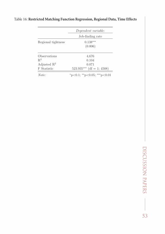
53

DISC

USSIO

N PAPER

STable 16: Restricted Matching Function Regression, Regional Data, Time Effects


∗∗∗p < 0.001, ∗∗p < 0.01, ∗p < 0.05



Dependent variable:

Job-finding rate


(0.008)


Note: ∗p<0.1; ∗∗p<0.05; ∗∗∗p<0.01


Dependent variable:

Job-finding rate


(0.006)


Note: ∗p<0.1; ∗∗p<0.05; ∗∗∗p<0.01

46

54

DP

/114

/201

9B. unrestricted versions of the testing

and estimation procedure for the fields of education and regional data

An unrestricted version of the testing and estimation procedure for the fields of education data is provided in Tables 17–23. This mirrors the structure presented in subsection 5.1.2. As the testing framework did not find evidence of time effects, the counterpart of Table 9 is not provided here.

Tables 24–29 present the unrestricted version of the testing and estimation procedure for the regional data that was outlined in subsection 5.1.3. The estimation of the overall tightness coefficient is unavailable for the case of time and two-way effects under fixed effects (within) estimation and the corresponding tables are not provided here. The estimated regional tightness coefficients for those two cases are respectively 0.14 and 0.05.

Table 17: Poolability Test (Unrestricted Version, Null Hypothesis: Identical Coefficients)

B. Unrestricted versions of the testing andestimation procedure for the fields of educationand regional data

An unrestricted version of the testing and estimation procedure for the fields ofeducation data is provided in Tables 17-23. This mirrors the structure presentedin subsection 5.1.2. As the testing framework did not find evidence of time effects,the counterpart of Table 9 is not provided here.Tables 24-29 present the unrestricted version of the testing and estimation

procedure for the regional data that was outlined in subsection 5.1.3. Theestimation of the overall tightness coefficient is unavailable for the case of timeand two-way effects under fixed effects (within) estimation and thecorresponding tables are not provided here. The estimated regional tightnesscoefficients for those two cases are respectively 0.14 and 0.05.


∗∗∗p < 0.001, ∗∗p < 0.01, ∗p < 0.05

Table 17: Poolability test (unrestricted version, null hypothesis: identicalcoefficients)


∗∗∗p < 0.001, ∗∗p < 0.01, ∗p < 0.05



∗∗∗p < 0.001, ∗∗p < 0.01, ∗p < 0.05


47






∗∗∗p < 0.001, ∗∗p < 0.01, ∗p < 0.05



∗∗∗p < 0.001, ∗∗p < 0.01, ∗p < 0.05



∗∗∗p < 0.001, ∗∗p < 0.01, ∗p < 0.05


47






∗∗∗p < 0.001, ∗∗p < 0.01, ∗p < 0.05



∗∗∗p < 0.001, ∗∗p < 0.01, ∗p < 0.05



∗∗∗p < 0.001, ∗∗p < 0.01, ∗p < 0.05


47

55

DISC

USSIO

N PAPER

STable 20: Lagrange Multiplier Test – Time Effects (Honda) for Balanced Panels

Model 1LM statistic −4.35∗∗∗p < 0.001, ∗∗p < 0.01, ∗p < 0.05




Dependent variable:

Job-finding rate

Sectoral tightness 0.015∗∗

(0.006)

Overall tightness 0.868∗∗∗

(0.014)

Constant 0.051(0.103)

Observations 1,848R2 0.718Adjusted R2 0.717F Statistic 2,343.540∗∗∗ (df = 2; 1845)

Note: ∗p<0.1; ∗∗p<0.05; ∗∗∗p<0.01

Table 22: Unrestricted matching function regression, fields of education data,individual effects

48






Dependent variable:

Job-finding rate


(0.006)


(0.014)

Constant 0.051(0.103)


Note: ∗p<0.1; ∗∗p<0.05; ∗∗∗p<0.01


48

Table 22: Unrestricted Matching Function Regression, Fields of Education Data, Individual Effects





Dependent variable:

Job-finding rate


(0.006)


(0.014)

Constant 0.051(0.103)


Note: ∗p<0.1; ∗∗p<0.05; ∗∗∗p<0.01


48

56

DP

/114

/201

9Table 23: Unrestricted Matching Function Regression,

Fields of Education Data, Two-way Effects

Dependent variable:

Job-finding rate


(0.005)


(0.027)

Constant 0.059(0.123)


Note: ∗p<0.1; ∗∗p<0.05; ∗∗∗p<0.01

Table 23: Unrestricted matching function regression, fields of education data, two-way effects


∗∗∗p < 0.001, ∗∗p < 0.01, ∗p < 0.05



∗∗∗p < 0.001, ∗∗p < 0.01, ∗p < 0.05



∗∗∗p < 0.001, ∗∗p < 0.01, ∗p < 0.05



∗∗∗p < 0.001, ∗∗p < 0.01, ∗p < 0.05


49

Table 24: Poolability Test (Unrestricted Version, Null Hypothesis: Identical Coefficients)

Dependent variable:

Job-finding rate


(0.005)


(0.027)

Constant 0.059(0.123)


Note: ∗p<0.1; ∗∗p<0.05; ∗∗∗p<0.01



∗∗∗p < 0.001, ∗∗p < 0.01, ∗p < 0.05



∗∗∗p < 0.001, ∗∗p < 0.01, ∗p < 0.05



∗∗∗p < 0.001, ∗∗p < 0.01, ∗p < 0.05



∗∗∗p < 0.001, ∗∗p < 0.01, ∗p < 0.05


49


Dependent variable:

Job-finding rate


(0.005)


(0.027)

Constant 0.059(0.123)


Note: ∗p<0.1; ∗∗p<0.05; ∗∗∗p<0.01



∗∗∗p < 0.001, ∗∗p < 0.01, ∗p < 0.05



∗∗∗p < 0.001, ∗∗p < 0.01, ∗p < 0.05



∗∗∗p < 0.001, ∗∗p < 0.01, ∗p < 0.05



∗∗∗p < 0.001, ∗∗p < 0.01, ∗p < 0.05


49


Dependent variable:

Job-finding rate


(0.005)


(0.027)

Constant 0.059(0.123)


Note: ∗p<0.1; ∗∗p<0.05; ∗∗∗p<0.01



∗∗∗p < 0.001, ∗∗p < 0.01, ∗p < 0.05



∗∗∗p < 0.001, ∗∗p < 0.01, ∗p < 0.05



∗∗∗p < 0.001, ∗∗p < 0.01, ∗p < 0.05



∗∗∗p < 0.001, ∗∗p < 0.01, ∗p < 0.05


49

57

DISC

USSIO

N PAPER

STable 27: Lagrange Multiplier Test –

Time Effects (Honda) for Balanced Panels

Dependent variable:

Job-finding rate


(0.005)


(0.027)

Constant 0.059(0.123)


Note: ∗p<0.1; ∗∗p<0.05; ∗∗∗p<0.01



∗∗∗p < 0.001, ∗∗p < 0.01, ∗p < 0.05



∗∗∗p < 0.001, ∗∗p < 0.01, ∗p < 0.05



∗∗∗p < 0.001, ∗∗p < 0.01, ∗p < 0.05



∗∗∗p < 0.001, ∗∗p < 0.01, ∗p < 0.05


49

Table 28: Hausman Test For Fixed vs. Random Effects


∗∗∗p < 0.001, ∗∗p < 0.01, ∗p < 0.05


Dependent variable:

Job-finding rate


(0.007)


(0.010)


Note: ∗p<0.1; ∗∗p<0.05; ∗∗∗p<0.01

Table 29: Unrestricted matching function regression, regional data, individualeffects

50

Table 29: Unrestricted Matching Function Regression, Regional Data, Individual Effects


∗∗∗p < 0.001, ∗∗p < 0.01, ∗p < 0.05


Dependent variable:

Job-finding rate


(0.007)


(0.010)


Note: ∗p<0.1; ∗∗p<0.05; ∗∗∗p<0.01

Table 29: Unrestricted matching function regression, regional data, individualeffects

50

Elements of the 1 lev banknote, issue 1999, are used in cover design.

ISBN 978-619-7409-15-4

labour market functioning and matching efficiency in

Documents