laboratory instruction manual -...

LABORATORY INSTRUCTION MANUAL

CIRCUIT THEORY & NETWORK LAB

EE 391

ELECTRICAL ENGINEERING DEPARTMENT

JIS COLLEGE OF ENGINEERING

(AN AUTONOMOUS INSTITUTE)

KALYANI, NADIA

CIRCUIT THEORY LAB. MANUAL EE 391

Page | 2

Stream: EE

Subject Name: CIRCUIT THEORY AND NETWORK LAB

Subject Code: EE391

LIST OF EXPERIMENTS

1. Transient response of R-L and R-C network: simulation with PSPICE/MATLAB

/Hardware

2. Transient response of R-L-C series and parallel circuit: Simulation with

PSPICE/MATLAB / Hardware

3. Study the effect of inductance on step response of series RL circuit in

MATLAB/HARDWARE.

4. Determination of Impedance (Z) and Admittance (Y) parameter of two port network:

Simulation / Hardware.

5. Frequency response of LP and HP filters: Simulation / Hardware.

6. Frequency response of BP and BR filters: Simulation /Hardware.

7. Generation of Periodic, Exponential, Sinusoidal, Damped Sinusoidal, Step, Impulse,

Ramp signal using MATLAB in both discrete and analog form.

8. Determination of Laplace transform and Inverse Laplace transform using MATLAB.

EE 391 CIRCUIT THEORY LAB. MANUAL

EE 391

Page | 3

EXPERIMENT NO : CKT /1

TITLE : TRANSIENT RESPONSE OF R-L AND R-C NETWORK: SIMULATION

WITH PSPICE/MATLAB /HARDWARE

OBJECTIVE : Study and obtain the transient response of a series R-C and series R-L circuit

using MATLAB.

THEORY:

Let us consider the R-C circuit as shown below:

Applying KVL, we obtain

1

( ) ( ) ( )v t Ri t i t dtC

Taking Laplace transform on both sides of the above equation,

1 ( ) (0 _)

( ) ( )I s q

V s RI sC s s

or, (0 _)( )

( ) ( ) CvI sV s RI s

sC s

Now as all initial conditions set equal to zero, i.e. (0 _) 0Cv , so the

equation becomes

( )

( ) ( )I s

V s RI ssC

or, 1

( ) ( )V s I s RsC


Page | 4

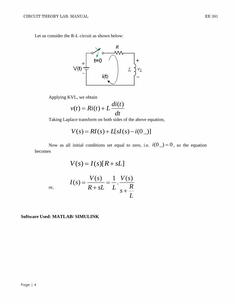
Let us consider the R-L circuit as shown below:


( )( ) ( )

di tv t Ri t L

dt


( ) ( ) [ ( ) (0_)]V s RI s L sI s i

Now as all initial conditions set equal to zero, i.e. (0 _) 0i , so the equation

becomes

( ) ( )[ ]V s I s R sL

or,

( ) 1 ( )( ) .

V s V sI s

RR sL Ls

L

Software Used: MATLAB/ SIMULINK


EE 391

Page | 5

Example 1: To simulate and study the transient response of a series R-C circuit using

MATLAB where R=200Ω, C=10µF for the following conditions:

1) source voltage is 40V DC with all initial conditions set equal to zero.

2) source voltage is a pulse signal with a period of 0s, width of 5ms, rise and fall

times of 1µs, amplitude of 20V and an initial value of 0V and all initial

conditions set equal to zero.

For Case - 1:-

( ) 40 ( )v t u t 40

( )V ss

Therefore,

40 40 1( ) . .

1 1( ) ( )

sCI s

s RRC s s

RC RC

Taking Inverse Laplace transform on both sides of the above equation,

1.40

( )t

RCi t eR

Putting 200R and 10C F , we get

500.40

( )200

ti t e

At 0t ,

40( ) A 200mA

200i t

At t , ( ) 0i t

At 2mst RC , ( ) 200 (37%) 74mAi t

Voltage drop across the resistor R is,

500. 500.40

( ) ( ) 200 . 40200

t tRV t Ri t e e

At 0t , ( ) 40VRV t

At t , ( ) 0RV t


Page | 6

The plot of ( )i t vs. t and ( )RV t vs. t are as follows:

Voltage drop across the capacitor C is,

500.( ) ( ) ( ) 40(1 )t

RCV t v t V t e

At 0t , ( ) 0CV t

At t , ( ) 40VCV t

The plot of ( )CV t vs. t is as follows:

For Case - 2:-

( ) 20[ ( ) ( 1)]v t u t u t

Therefore,

20( ) (1 )sV s e

s


EE 391

Page | 7

and,

20 (1 ) 1 20 1( ) . .

1 1 1( ) ( ) ( )

s ssC e eI s

s RsRC s s s

RC RC RC

Taking Inverse Laplace transform on both sides of the above equation,

1 1. .( 1)20

( ) ( ) ( 1)t t

RC RCi t e u t e u tR

Putting 200R and 10C F , we get

500. 500.( 1)20

( ) ( ) ( 1)200

t ti t e u t e u t

At 0t ,

20( ) A 100mA

200i t

At t , ( ) 0i t


500. 500.( 1)20

( ) 200 ( ) ( 1)200

( ) t t

RV Ri t e u t e u tt

or, 500. 500.( 1)20 ( ) ( 1)( ) t t

RV e u t e u tt

At 0t , ( ) 20VRV t

At t , ( ) 0RV t

Voltage drop across the capacitor C is,

500. 500.( 1)( ) ( ) ( ) 20(1 ) ( ) 20(1 ) ( 1)t t

RCV t v t V t e u t e u t

At 0t , ( ) 0CV t

At t , ( ) 0CV t

At 5mst T , ( ) 18.36VCV t


Page | 8

SIMULATION DIAGRAM:

For Case - 1:-

For Capacitor C1: IC=0V

For Analysis Setup:

Transient:-

Print Step : 0s

Final Time : 20ms

Simulate the individual circuits and draw the plot of ( )i t vs. t , ( )RV t vs. t and ( )CV t vs. t .

For Case - 2:-

For Capacitor C1: IC=0V

For source voltage VPULSE:

V1: 0V; V2: 20V

TD: 0s

TR: 1µs; TF: 1µs

PW: 5ms; PER: 0s

For Analysis Setup:

Transient:-

Print Step : 0s

Final Time : 16ms

Simulate the individual circuits and draw the plot of ( )i t vs. t , ( )RV t vs. t and ( )CV t vs. t .


EE 391

Page | 9

Example 2: To simulate and study the transient response of a series R-L circuit using

PSPICE where R=100Ω, L=10mH for the following conditions:

1) source voltage is 10V DC with all initial conditions set equal to zero.

2) source voltage is 10V DC with initial condition (0 _) 20mALi .

For Case - 1:-

)(10)( tutv 10

( )V ss

Therefore,

10

1 1 10 10 1 1( ) .

( )

sI sR R RL L R s

s s s sL L L

Taking inverse Laplace transform on both sides of the above equation,

.10( ) 1

Rt

Li t eR

Putting 100R and 10L mH , we get

41010

( ) 1100

ti t e

At 0t , ( ) 0i t

At t , 10

( ) A 100mA100

i t

At 100μsL

tR

, ( ) 100 (63%) 63mAi t


4 410 . 10 .10( ) 100 (1 ) 10(1 )

100( ) t t

RV Ri t e et

At 0t , ( ) 0RV t

At t , ( ) 10VRV t


Page | 10

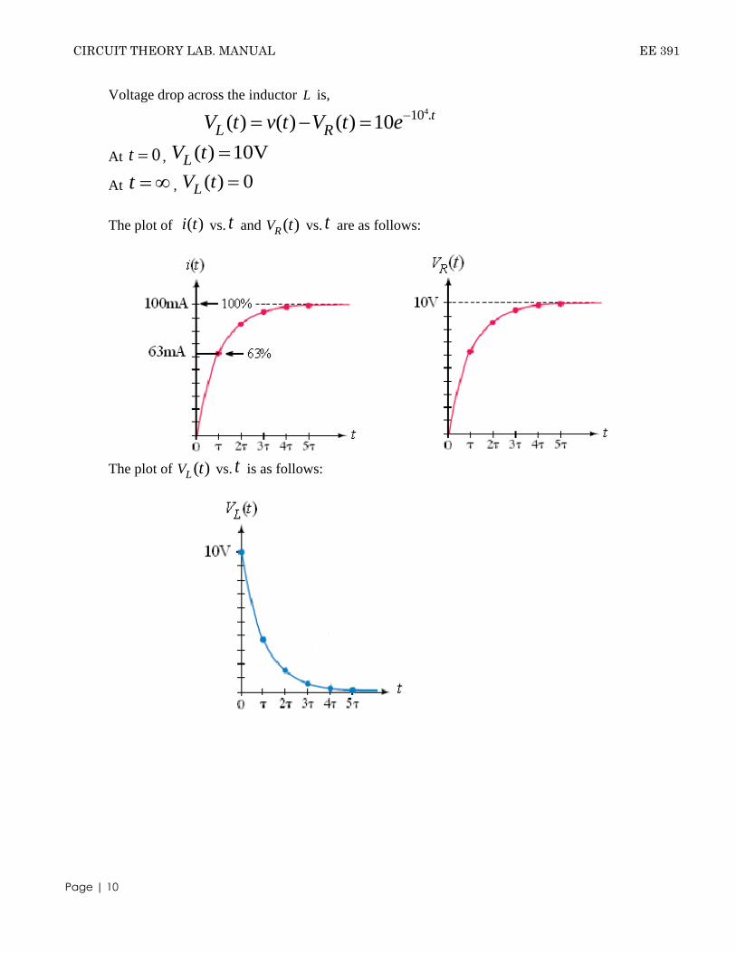
Voltage drop across the inductor L is,

410 .( ) ( ) ( ) 10 t

L RV t v t V t e

At 0t , ( ) 10VLV t

At t , ( ) 0LV t

The plot of ( )i t vs. t and ( )RV t vs. t are as follows:

The plot of ( )LV t vs. t is as follows:


EE 391

Page | 11

For Case - 2:-

)(10)( tutv and (0 _) 20mALi

10

( )V ss

3( ) ( ) [ ( ) 20 10 ]V s RI s L sI s

or, 41020 10 ( )

RLI s s

s L

or,

3

4 4

0.02 10( )

10 ( 10 )I s

s s s

Taking inverse Laplace transform on both sides of the above equation,

410 .( ) 0.1 0.08 ti t e

At 0t , ( ) 20mAi t

At t , ( ) 100mAi t


4 410 . 10 .( ) 100 ( ) 100(0.1 0.08 ) 10 8( ) t t

RV Ri t i t e et

At 0t , ( ) 2VRV t

At t , ( ) 10VRV t

Voltage drop across the inductor L is,

410 .( ) ( ) ( ) 8 t

L RV t v t V t e

At 0t , ( ) 8VLV t

At t , ( ) 0LV t


Page | 12

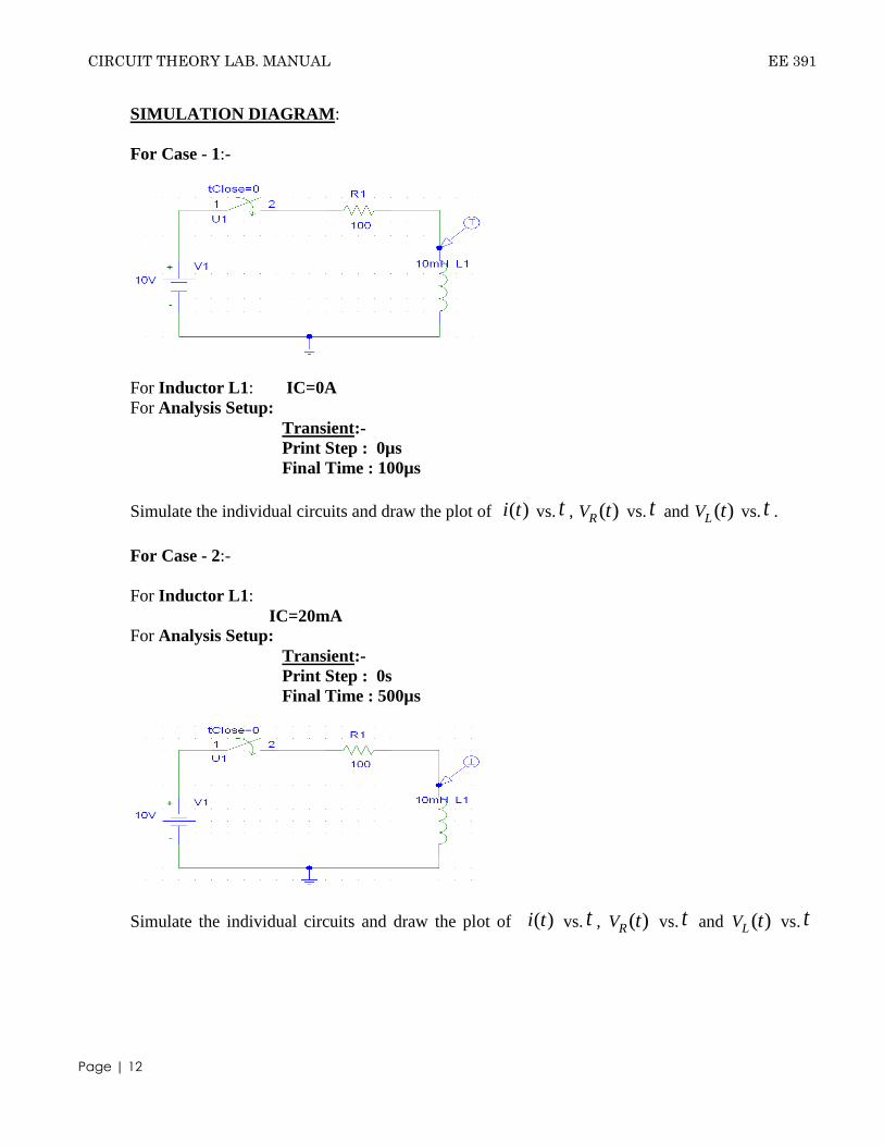
SIMULATION DIAGRAM:

For Case - 1:-

For Inductor L1: IC=0A

For Analysis Setup:

Transient:-

Print Step : 0µs

Final Time : 100µs

Simulate the individual circuits and draw the plot of ( )i t vs. t , ( )RV t vs. t and ( )LV t vs. t .

For Case - 2:-

For Inductor L1:

IC=20mA

For Analysis Setup:

Transient:-

Print Step : 0s

Final Time : 500µs

Simulate the individual circuits and draw the plot of ( )i t vs. t , ( )RV t vs. t and ( )LV t vs. t

EE 391 CIRCUIT THEORY LAB. MANUAL EE 391

Page | 13

EXPERIMENT NO : CKT/2

TILLE : TRANSIENT RESPONSE OF R-L-C SERIES AND PARALLEL

CIRCUIT SIMULATION WITH PSPICE/MATLAB / HARDWARE

OBJECTIVE : To determine

I. Transient response of a series R-L-C circuit, excited by a unit step input

using MATLAB.

II. Transient response of a R-L-C parallel circuit, excited by a unit step input

using MATLAB.

THEORY: Let us consider the R-L-C circuit as shown below:


( ) 1( ) ( ) ( )

di tv t Ri t L i t dt

dt C


(0 _)( )( ) ( ) [ ( ) (0 _)] CvI s

V s RI s L sI s isC s

Now as all initial conditions set equal to zero, i.e. (0 _) 0i and (0 _) 0Cv , so

the equation

becomes,

1( ) ( )V s I s R sL

sC


Page | 14

Here, ( ) ( )v t u t 1

( )V ss

Therefore,

1 1( )I s R sL

s sC

or, 2

1

( )1

LI sR

s L sL LC

The roots of the denominator polynomial of the above equation are,

2 10

Rs L s

L LC

or,

2

1 2

1

2 4

R Rs

L L LC

and

2

2 2

1

2 4

R Rs

L L LC

Let 0

1

LC

and 02

R

L

2

R C

L

Now,

1 2 2 1

1 2 1 2

1 11

( ) ( )( )

( )( ) ( ) ( )

L s s L s sLI ss s s s s s s s

or, 21 20

1 1 1( )

( ) ( )2 1I s

s s s sL


Page | 15

Taking inverse Laplace Transform on both sides,

2 20 0 0

2

0

1 11( )

2 1

t t ti t

Le e e

Case - 1:-

R 2L

C

i.e. 1

200

2

0

1( ) sin 1

1

ti t t

Le

The network is then said to be Under Damped or Oscillatory.

Case - 2:-

R 2L

C

i.e. 1

0

1( ) .

ti t t

Le

The network is then said to be Critically Damped.

Case - 3:-

R 2L

C

i.e. 1

200

2

0

1( ) sinh 1

1

ti t t

Le

The network is then said to be Over Damped.


Page | 16

The current response for the above three cases is shown in the figure below:


Page | 17

Example 1: Obtain the transient response of a series RLC circuit, excited by a unit step input,

using MATLAB where L 8mH and C 2 Fµ for the following conditions:

1) R 2L

C , under damped case where R 1

2) R 2L

C , critically damped case where R 4

3) R 2L

C , over damped case where R 6

SIMULATION DIAGRAM:

For Case - 1:-

For

Inductor L1: IC=0A

Capacitor C1: IC=0V

For Analysis Setup:

Transient:-

Print Step : 0µs

Final Time : 100µs

Simulate the circuit and draw the plot of ( )i t vs. t .

Note the value of the first peak of the current response.

For Case - 2:-

For

Inductor L1: IC=0A

Capacitor C1: IC=0V


Page | 18

For Analysis Setup:

Transient:-

Print Step : 0µs

Final Time : 50µs



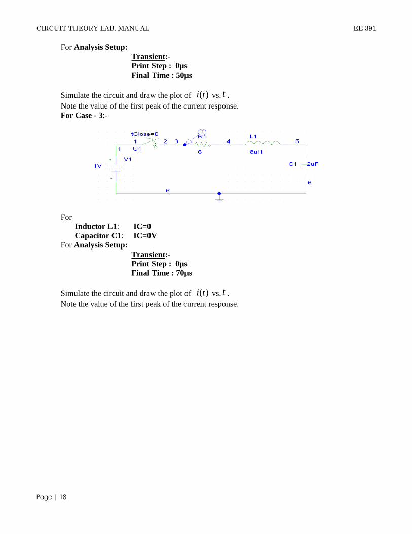
For Case - 3:-

For

Inductor L1: IC=0

Capacitor C1: IC=0V

For Analysis Setup:

Transient:-

Print Step : 0µs

Final Time : 70µs




Page | 19


TILLE : STUDY THE EFFECT OF INDUCTANCE ON STEP RESPONSE OF

SERIES RL CIRCUIT IN MATLAB/HARDWARE.


I. The effect of inductance on step response of series RL circuit.

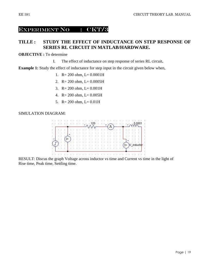
Example 1: Study the effect of inductance for step input in the circuit given below when,

1. R= 200 ohm, L= 0.0001H

2. R= 200 ohm, L= 0.0005H

3. R= 200 ohm, L= 0.001H

4. R= 200 ohm, L= 0.005H

5. R= 200 ohm, L= 0.01H

SIMULATION DIAGRAM:

RESULT: Discus the graph Voltage across inductor vs time and Current vs time in the light of

Rise time, Peak time, Settling time.


Page | 20


TILLE : DETERMINATION OF IMPEDANCE (Z) AND ADMITTANCE (Y)

PARAMETER OF TWO PORT NETWORK: SIMULATION /

HARDWARE.


I. The open circuit impedance parameters of the ‘T’ network.

II. The short circuit admittance parameters of the ‘π’ network

THEORY: Let us consider a linear passive two port network as shown in figure below:

We know, V1= Z11 I1 + Z12 I2 ……………(1)

V2= Z21 I1 + Z22 I2 ……………(2)

Z-parameters are obtained by making either terminals 11’ open circuited or terminals 22’

open circuited.

0

1

111 2 I

I

VZ

is called the input impedance or driving point impedance with output open circuited.

0

1

221 2 I

I

VZ

is called the forward transfer impedance with output open circuited.

0

2

112 1 I

I

VZ

is called the reverse transfer impedance with output open circuited.

0

2

222 1 I

I

VZ


Page | 21

is called the output impedance with input open circuited.

The Y-parameters of this network can be obtained by expressing I1 and I2 in terms of V1

and V2.

I1= Y11 V1 + Y12 V2 ……………(1)

I2= Y21 V1 + Y22 V2 ……………(2)

Y-parameters are obtained by making either terminals 11’ short circuited or terminals

22’ short circuited.

0

1

1

11 2 V

V

IY

is called the input admittance or driving point admittance with output short circuited.

0

1

2

21 2 V

V

IY

is called the forward transfer admittance with output short circuited.

0

2

112 1 V

V

IY

is called the reverse transfer admittance with input short circuited.

0

2

2

22 1 V

V

IY

is called the output admittance with input short circuited.


Page | 22

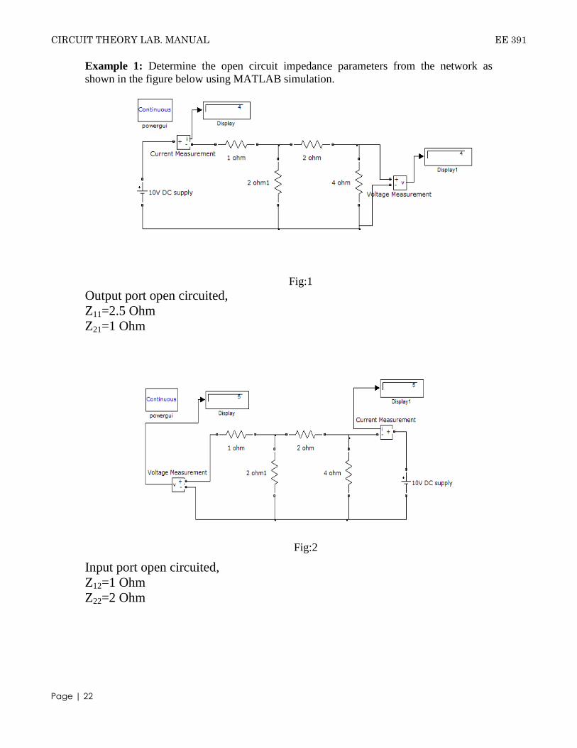
Example 1: Determine the open circuit impedance parameters from the network as

shown in the figure below using MATLAB simulation.

Fig:1

Output port open circuited,

Z11=2.5 Ohm

Z21=1 Ohm

Fig:2

Input port open circuited,

Z12=1 Ohm

Z22=2 Ohm


Page | 23

Example 2: Determine the short circuit admittance parameters from the network as

shown in the figure below using MATLAB simulation.

Applied voltage at output port is 10 V.

Fig:1

For the input port short circuited, we have

Y22=0.3125 mho

Y12=0.1875 mho

Applied voltage at input port is 10 V.

Fig:2

For the output port short circuited,

Y11=0.3125 mho

Y21=0.1875 mho


Page | 24

Example 3: Determine the short circuit admittance parameters from the network as shown in the figure

below using MATLAB simulation.

Applied voltage at input port is 10 V.

Fig:1

For the output port short circuited,

Y11=0.375 mho

Y21= 0.25 mho

Applied voltage at output port is 10 V.

Fig:2

For the input port short circuited,

Y22=1 mho

Y12= 0.25 mho


Page | 25


TILLE : FREQUENCY RESPONSE OF LP AND HP FILTERS: SIMULATION

/ HARDWARE.

OBJECTIVE : To study the frequency response of Low Pass and High Pass filter using MATLAB.

Example 1: Show the frequency response of a low pass filter.

Matlab Code : f=0:1:10^6

r1=10000

rf=1000

r=15900

c=0.01*10^-6

af=(1+rf/r1)

fc=1/(2*pi*r*c)

a=f/fc

acl_lp=af./sqrt(1+a.*a)

semilogx(acl_lp)

xlabel('frequency----->')

ylabel('gain--------->')

title('frequency response of low pass filter')

grid

Output :


Page | 26

Example 1: Show the frequency response of a high pass filter.

Matlab Code : f=[0:1:10^6]; r1=10000; rf=1000; r=15900; c=0.01*10^(-6); af=(1+rf/r1); fc=1/(2*pi*r*c); a=f/fc; acl_lp=af.*a./sqrt(1+a.*a); semilogx(acl_lp) xlabel('frequency----->') ylabel('gain--------->') title('frequency response of high pass filter') grid

Output :


Page | 27


TILLE : GENERATION OF PERIODIC, EXPONENTIAL, SINUSOIDAL,

DAMPED SINUSOIDAL, STEP, IMPULSE, RAMP SIGNAL USING

MATLAB IN BOTH DISCRETE AND ANALOG FORM.

OBJECTIVE : To generate

I. Normal sinusoidal signal

II. Under damped signal

III. Over damped signal

IV. Discrete sinusoidal signal

V. Discrete damped sinusoidal signal

VI. Unit step function-1

VII. Unit step function-2

VIII. Ramp wave

IX. Impulse wave

Example 1: Generate normal sinusoidal signal

Matlab Code:

f=input('enter the freq:'); n=input('enter the length:') w=2*pi*f; t=0:0.01:10 y=sin(w*t) plot(t,y); xlabel('time in sec...........>'); ylabel('amplitude in cm..........>'); title('NORMAL SINUSODIAL SIGNAL'); grid on;

Output :

Enter the frequency: 1 Enter the length: 10

0 1 2 3 4 5 6 7 8 9 10-1

-0.8

-0.6

-0.4

-0.2

0

0.2

0.4

0.6

0.8

1

time in sec...........>

amplitu

de in c

m.......

...>

NORMAL SINUSODIAL SIGNAL


Page | 28

Example 2: Generate Under damped signal

Matlab Code:

a=input('enter the damping costant:'); l=input('enter the length:'); t=0:0.1:10 y=exp(-a*t); plot(t,y); xlabel('time in sec'); ylabel('amplitude in cm.'); title(‘UNDER DAMPED SIGNAL'); grid on;

Output :

Enter the damping constant: 0.5 Enter the length: 10

0 1 2 3 4 5 6 7 8 9 100

0.1

0.2

0.3

0.4

0.5

0.6

0.7

0.8

0.9

1

time in sec

ampl

itude

in c

m.

UNDER DAMPED SIGNAL


Page | 29

Example 3: Generate Over damped signal

Matlab Code:

a=input('enter the damping costant:'); l=input('enter the length:'); y=exp(a*t); t=0:0.1:10 plot(t,y); xlabel('time in sec'); ylabel('amplitude in cm.'); title('OVER DAMPED SIGNAL'); grid on;

Output :

Enter the damping constant: 0.5 Enter the length: 10

0 1 2 3 4 5 6 7 8 9 100

50

100

150

time in sec

ampl

itude

in c

m.

OVER DAMPED SIGNAL


Page | 30

Example 4: Discrete Sinusoidal signal

Matlab Code:

f=input('enter the freq:'); n=input('enter the length:'); w=2*pi*f; t=0:0.1:10 y=sin(w*t) stem(t,y); xlabel('time in sec...........>'); ylabel('amplitude in cm.............>'); title('DISCRETE SINUSODIAL SIGNAL'); grid on;

Output :

Enter the frequency: 1 Enter the length: 10

0 1 2 3 4 5 6 7 8 9 10-1

-0.8

-0.6

-0.4

-0.2

0

0.2

0.4

0.6

0.8

1

time in sec...........>

am

plitu

de in c

m..

....

....

...>

DISCRETE SINUSODIAL SIGNAL


Page | 31

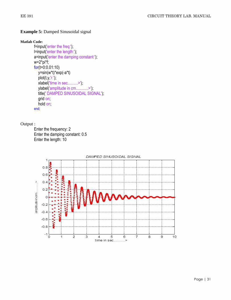
Example 5: Damped Sinusoidal signal

Matlab Code:

f=input('enter the freq:'); l=input('enter the length:'); a=input('enter the damping constant:'); w=2*pi*f; for(t=0:0.01:10) y=sin(w*t)*exp(-a*t) plot(t,y,'r.'); xlabel('time in sec..........>'); ylabel('amplitude in cm............>'); title(' DAMPED SINUSOIDAL SIGNAL'); grid on; hold on; end;

Output :

Enter the frequency: 2 Enter the damping constant: 0.5 Enter the length: 10


Page | 32

Example 6: Generate Unit step function

Matlab Code:

t=0:0.1:10; t0=2; y=0*(t<t0)+1*(t>=t0) plot(t,y); xlabel('time...............>'); ylabel('amplitude.............>'); title('UNIT STEP FUNCTION '); grid on;

Output :

0 1 2 3 4 5 6 7 8 9 100

0.1

0.2

0.3

0.4

0.5

0.6

0.7

0.8

0.9

1

time...............>

am

plit

ude..

....

....

...>

UNIT STEP FUNCTION


Page | 33

Example 7: Generate Unit step function 2

Matlab Code:

t=0:0.1:10; y=1*(t>=1)-1*(t>=3); plot(t,y); xlabel('Time'); ylabel('Amplitude'); title('UNIT STEP SIGNAL'); grid on;

Output :

0 1 2 3 4 5 6 7 8 9 100

0.1

0.2

0.3

0.4

0.5

0.6

0.7

0.8

0.9

1

Time

Am

plit

ude

UNIT STEP SIGNAL


Page | 34


TILLE : DETERMINATION OF LAPLACE TRANSFORM AND INVERSE

LAPLACE TRANSFORM USING MATLAB.

OBJECTIVE : To find the Laplace & Inverse Laplace transform by using Matlab commands.

THEORY:

The mathematical expression for Laplace transform is

0

*)()()( dtetfsFtLf st

The term “Laplace transform of f(t)” is used for the letter Lf(t). The time function f(t) is

obtained back from the Laplace transform by a process called inverse Laplace transformation

and denoted by L-1

thus

L-1

[Lf(t)]=L-1

[F(s)]=f(t). The time function f(t) and its Laplace transform F(s) are a transform pair.

Derivation of Laplace transform:-

Laplace transform of eat is

as

dtedteeeL tsastatat

1.][

0

)(

0

Now put a=jw

)(

1]sin[cos][

22

s

js

jstjtLeL tj

22][cos

s

stL & 22

][sin

stL

Now, )()]([ asFtfeL at

2

0

1.][

sdtettL st

as

dtedteeeL tsastatat

1.][

0

)(

0

)()]([ asFtfeL at , ttf )( & a= -3


Page | 35

2

1)(

ssF

2

3

)3(

1].[

steL t

]}[][]1[{1

]/)1[(2

2 atatatat teaLeLLa

aateeL

])(

11[

122 as

a

assa

)()]([ asFtfeL at , ttf sin)( , 3a & 10

22)(

ssF

100)3(

10]10sin.[

2

3

steL t

Derivation of inverse Laplace transform:-

)()]([1 tfsFL

ate

asL

]1

[1

1

112

1)1(

2)(

222

ssss

C

s

B

s

A

ss

ssF

)2

(2212)]([2/2/

2/1tt

tt eeetetsFL

)2/sinh(22 2/ tet t

3

116

5)(

sssF

tets

LLs

LsFL 31111 )(165]3

1[]16[]

5[)]([


Page | 36

Laplace Transform:

Example 1: f(t)=e-5t

Program:

Syms t s

ft=exp(-5*t)

fs=laplace(ft)

Output:

fs=1/(s+5)

Example 2: f(t)=e3t

Program:

Syms t s

ft=exp(3*t)

fs=laplace(ft)

Output:

fs=1/(s-3)

Example 3: f(t)=sin2t

Program:

Syms t s

ft=sin(2*t)

fs=laplace(ft)

output:

fs=2/(s2+4)

Example 4: f(t)=cos5t

Program:

Syms t s

ft=cos(5*t)

fs=laplace(ft)

Output:

fs=s/(s2+25)

Example 5: f(t)=t6

Program:

Syms t s

ft=t6

fs=laplace(ft)

output:

fs=720/s7


Page | 37

Example 6: f(t)=t2sin6t

Program:

Syms t s

ft=t^2*sin(6*t)

fs=laplace(ft)

output:

fs=36*(s^2-12)/(s^2+36)^3

Example 7: f(t)=e3tsin2t

Program:

Syms t s

ft=exp(3*t)*sin(2*t)

fs=laplace(ft)

output:

fs=2/(s^2-6*s+13)


cos7t

Program:

Syms t s

ft=exp(-3*t)*cos(7*t)

fs=laplace(ft)

output:

fs=(s+3)/(s^2+6*s+58)


sin4t

Program:

Syms t s

ft=exp(-2*t)*sin(4*t)

fs=laplace(ft)

output:

fs=4/(s^2+4*s+20)

Example 10: f(t)=e7tcos2t

Program:

Syms t s

ft=exp(7*t)*cos(2*t)

fs=laplace(ft)

output:

fs=(s-7)/(s^2-14*s+53)


Page | 38

Inverse Laplace Transform:

Example 1: f(s)=s+1/s(s+2)(s+3)

Program:

Syms t s

fs=(s+1)/(s^3+5*s^2+6*s)

ft=ilaplace(fs)

output:

ft=-2/3*exp(-3*t)+1/2*exp(-2*t)+1/6

Example 2: f(s)=(s3+3s

2+4s+4)/(s+1)(s+4)

Program:

Syms t s

fs=(s^3+3*s^2+4*s+4)/(s^2+5*s+4)

ft=ilaplace(fs)

output:

ft=dirac(1,T)-2*dirac(t)+2/3*exp(-t)+28/3*exp(-4*t)

Example 3: f(s)=3/s2+8s+25

Program:

Syms t s

fs=3/( s^2+8*s+25)

ft=ilaplace(fs)

output:

ft=exp(-4*t)*sin(3*t)

Example 4: f(s)=s/s2+a

2

Program:

Syms a t s

fs=s/(s^2+a^2)

ft=ilaplace(fs)

output:

ft=cos(a*t)

Example 5: f(s)=1/s+a

Program:

Syms a t s

fs=1/(s+a)

ft=ilaplace(fs)

output:

ft=exp(-a*t)


Page | 39

laboratory instruction manual -...

Documents