Laboratory class 5

Determination of thermal stability of dielectrics Aims of the class: 1. To study the method of determination thermal stability of different insu-

lating materials by means of Martens furnace. 2. To determine the grade of thermal stability of thermoplastic polymers.

Theoretical fundamentals of dielectrics thermal stability determination Thermal stability of a dielectric is its ability to withstand both short-term

and long-term effect of high temperature without significant reduction of its me-chanical and electrical properties.

Elevated value of a dielectrical artilce thermal stability permits to de-crease its overall dimensions, mass and cost. Especially it is important for air-craft and spacecraft equipment.

By there behavior at heating electrotechnical materials can be classified as thermoplastic, thermo-stable and thermosetting.

Thermoplastic materials are ones having linear or low-branched ar-rangement, which soften at heating and even can melt transferring to viscous state and then after cooling become solid. This behavior is repeated at multiple heating and consequent cooling.

Thermo-stable materials have cross-linked grid microstructure. They don’t soften at heating even up to decomposition (or burning) temperature lev-el. In process of decomposition they absorb relatively high heat quantity there-fore can be recommended for thermally-stable ablation coatings.

Thermosetting materials are ones having linear molecular arrangement, which soften at heating, melt, transfer to viscous state and then have obtained cross-linked molecular arrangement with thermo-stable macro properties due to irreversible chemical reaction.

Upper allowable level of operating temperature for above-mentioned materials is defined by temperature after which visible and significant reduction of electrical and mechanical properties can be observed.

International Electrical Commission (IEC) classifies dielectrics by upper level of operational temperature as following seven grades: Grade U Grade A Grade E Grade B Grade F Grade H Grade C

up to 90° up to 105° up to 120° up to 130° up to 155° up to 180° > 180° Lower allowable level of operating temperatures (below than zero) is

defined by conditions of required elasticity, viscosity, flexibility, mechanical strength and resistance to cracks appearing at bending.

Thermal resistance of thermosetting and non-organic dielectrics corre-sponds to temperatures of visible growth of tangent of dielectrical losses or de-creasing of specific volumetric electrical resistance.

Thermal resistance of liquid dielectrics is defined by either the tempera-ture of flashing (burning) of their vapor mixture with air or by the temperature of a liquid ignition.

Thermal resistance of thermoplastic dielectrics is defined by origination of mechanical strain at tension, bending or by special needle penetration inside of material.

Thermal resistance of low-melting materials (paraffin, ceresin, ozocerite, bitumen etc.) is defined by the method of “ring and ball”.

Allowable operational temperature of electrical-insulating materials has to be always less than the temperature of melting, softening of ignition of vapor to ensure required level of mechanical strength, long-term operation and durability of an article.

The important parameter of resistance to sharp temperature changing or “thermal impact” is used for characterization of brittle insulators thermal stability (inorganic glass, ceramics, sitals etc):

σ λα

b m

p

F=E C

, (7.1)

where α – thermal coefficient of linear expansion; σb– ultimate strength of a

material at tension; E– elasticity modulus; λm – thermal conductivity coefficient;

pC – specific heat capacity.

The aim of the work is to determine the thermal stability grade of different thermoplastic materials by means of Martens furnace. Thermal stability is de-fined by the temperature at which bending stress σ

bend=5 MPa (50 kg/cm2)

causes visible deformation of standard specimen and the rate of temperature

increasing equal to 1°C per minute. Martens furnace consists of loading panel and thermostat with tempera-

ture regulator (Fig. 7.1). Loading panel permits to load three specimens simul-taneously. It contains lower supporting devices for specimens clamping and upper fixtures for loading specimens with bending moment.

Figure 7.1 The scheme of dielectric specimen testing The distance between clamping screws and panel contacts has to be

equal to 6±1 mm. Then panel with specimens has to be placed inside of ther-mostat and connect contacts of sound and light signalization to each specimen. Thermostat is the furnace equipped with thermal insulation, two thermometers, door with transparent screen and auxiliary lamp. Thermal regulator works au-tomatically and is equipped with switcher and thermal gage. Thermal gage con-tains quartz rod placed inside copper tube. At heating copper tube expands and interacts with quartz rod. As a result of heating reversed piezo-effect occurs in

the rod permitting to regulate the rate of furnace heating – 50°C per hour.

Procedure of the work 1. Install specimens vertically in lower clamps of testing facility. 2. Join loading levers on the upper edges of specimens to guarantee

spacing between contacts equal to 6±1 mm. 3. Install panel with specimens to the furnace to create contact between

specimens and furnace. 4. Attach contacts of signalization to each specimen. 5. Install thermometers left (vertical) and right (sloped) in such way to at-

tach mercury balls in each thermometer: the first one – to the upper edge of a specimen, the second one – to the lower edge of specimen.

6. Close Martens furnace and switch it on. 7. Make reading of temperature level (from both thermometers) at the

moment of contacts attaching (this moment is accompanied with sound and light signals).

8. Calculate average temperature

cp 1 2+T =(T T ) / 2 . (7.2)

9. Determine the grade of testing materials thermal stability. 10. Insert results of testing to the table 7.1 Table 7.1 – Results of measuring Material

1T , °C

2T , °C cpT , °C Thermal stability grade

11. Make the sketch of specimens loading and calculate bending mo-ment.

The content of the report

1. The aim of the work.

2. Information about testing materials. 3. The scheme of dielectrics testing on thermal stability by Martens meth-

od. 4. Results of thermal stability measuring (table 7.1). 5. Conclusions.

Checking-up problems 1. What is the difference between thermoplastic and thermosetting dielec-

trics? 2. Give the definition of dielectric thermal stability. 3. How to determine thermal stability of a dielectric by Martens method? 4. How to determine thermal stability of thermosetting dielectrics? 5. Explain the difference in thermal stability of several tested materials.

Laboratory class 6

Studying influence of temperature on resistance of conductors and semi-conductors

Aims of the work: 1. To study methods of measuring resistance of conductors and semi-

conductors. 2. To determine dependence of conductors and semi-conductors re-

sistance on temperature. 3. To calculate value of thermal coefficient of resistance for conductors

and semi-conductors.

Theoretical fundamentals Conductors and semi-conductors are widely used in different radio-

technical devices of aircrafts, spacecrafts and other objects of national econo-my. The major field of their application is manufacturing of resistors, conduc-tors, electrical contacts, diodes, triodes, thermistors and other devices.

Main electrical characteristics of semi-conductors are specific resistance

ρ and thermal coefficient of specific resistance ρα .

Specific resistance ρ [Ohm·m] of a conductor having electrical resistance R, length ℓ and cross-section S can be calculated as

ρ�

S= R . (8.1)

It can be found from the electronic theory of metals that specific re-

sistance of metal conductor can be estimated by means of Zommerfeld’s for-mula:

2

2m *=

n e

µρ

�, (8.2)

where m * – electron mass; µ– average speed of electron movement inside

metal conductor; n– quantity of free electrons per unit volume of conductor; �– average free path length of electron.

For majority of conductors average speed of electron heat movement is approximately the same and concentrations of free electrons differs negligibly. This is why the value of specific resistance depends mainly of average free path length of electron in a conductor.

Total resistance of metals and alloys can be considered as a sum of two components:

ρ ρ ρht res= + , (8.3)

where ρht – resistance stipulated by electrons dispersion on heat oscillations of

crystalline lattice; ρres– residual resistance related to electrons dispersion on

structural imperfections. All pure metals with regular crystalline lattice have minimal specific re-

sistance ρ and all alloys always have elevated values of ρ comparing with al-

loy components. This fact can be explained as following: average free path of electrons in alloys becomes less due to distortions of crystalline lattice.

At conductors heating the amplitude of heating oscillations of crystalline lattice nodes increases creating more quantity of irregularities on electrons paths. Therefore the length of electron free path decreases. The electrons con-centration n doesn’t depend on conductor temperature. Finally in accordance with formula (8.2) a conductor specific resistance increases at heating.

For relatively narrow temperature ranges dependence of specific re-sistance on temperature can be considered as piecewise-linear one:

ρρ ρ α ∆t 0= (1+ T) , (8.4)

where ∆T – temperature range; ρ0 – specific resistance of a conductor at the

temperature range beginning. The value of ρα characterizes changing of specific resistance at tempera-

ture changing on one degree and is known as coefficient of specific electri-cal resistance (measuring units – degree-1):

ρ

ρ ρα

ρ ∆t 0

0

-=

T, (8.5)

Thermal coefficients for pure metals are always more than for their alloys and close to 1/273, i.e. ρα ≈ 0.004 1/K. Thermal coefficients for definite alloys

can be very low and even negative. Many chemical elements and compounds are semi-conductors and by

electrical conductivity occupy intermediate position between metals and dielec-

trics. The range of electrical conductivity changing for semi-conductors is quite wide ρ =10-5…107 Ohm·m. The distinctive feature of semi-conductors from oth-

er materials is their strong dependence of electrical resistance on both concen-tration and types of impurities and such external energy effects as temperature, illumination etc.

The conductivity of chemically pure semi-conductors is known as proper conductivity and such semi-conductors are called as proper semi-conductors. Examples of proper semi-conductors are chemically pure germa-nium, silicon, selenium and compounds PbS, InSb, GaAs, CdS.

Conductivity of semi-conductors is very sensitive even to small amount of impurities. For example, introduction of 0,001% of boron to the silicon increas-es its conductivity in 1000 times. Conductivity of semi-conductors stipulated by presence of impurities is known as impurity conduction (extrinsic conduction) and correspondent semi-conductors are known as impurity (extrinsic) semi-conductors.

For manufacturing of semi-conducting devices only impurity semi-conductors are used.

Let’s consider influence of temperature on electrical conductivity of impu-rity semi-conductor. Impurity atoms obtain auxiliary energy for their ionizing at semi-conductor heating. At impurity atoms ionizing concentration of n and p charge carriers becomes more (Fig. 8.1, a). As a result specific resistance de-creases (see formula (8.2)).

Further temperature elevation permits to reach such level of energy at which proper conduction of semi-conductor occurs (Fig. 8.1, b).

a b

Fig. 8.1. Energy diagram of a semi-conductor Strictly speaking at elevated temperature semi-conductor transfers to off-

nominal regime of operation. The temperature at which off-nominal regime oc-

curs depends on the width of restricted zone and limits the upper operating temperature of the semi-conductor device. For relatively narrow temperature ranges the exponential dependence of specific resistance of semi-conductor on temperature can be used:

∆

ρ

Elim2KT= Ae ,

where ∆ limE – the width of restricted zone; K– Boltzmann’s constant; T– tem-

perature, K; A– constant of a material. Thus majority of semi-conductors at heating loss electrical resistance due

to increasing of charge carriers concentration. The distinctive feature of semi-conductors to change resistance is used in

such devices as thermistors. Thermistors are volumetric semi-conducting re-sistance high negative thermal coefficient

ρα2

B= -

T, (8.6)

where B=∆

−lim 1 2 1

2 1 2

E T T R= ln

2K T T R; 1T , 2T – initial and final temperatures; 1R , 2R –

resistance at the beginning and at the end of temperature range. Generally thermal coefficient of semi-conductors is not constant.

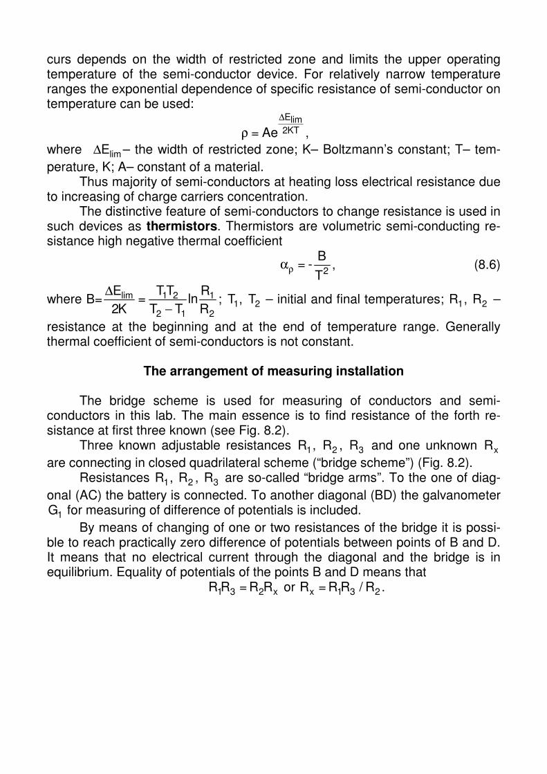
The arrangement of measuring installation

The bridge scheme is used for measuring of conductors and semi-

conductors in this lab. The main essence is to find resistance of the forth re-sistance at first three known (see Fig. 8.2).

Three known adjustable resistances 1R , 2R , 3R and one unknown xR

are connecting in closed quadrilateral scheme (“bridge scheme”) (Fig. 8.2). Resistances 1R , 2R , 3R are so-called “bridge arms”. To the one of diag-

onal (AC) the battery is connected. To another diagonal (BD) the galvanometer

1G for measuring of difference of potentials is included.

By means of changing of one or two resistances of the bridge it is possi-ble to reach practically zero difference of potentials between points of B and D. It means that no electrical current through the diagonal and the bridge is in equilibrium. Equality of potentials of the points B and D means that

1 3 2 xR R = R R or x 1 3 2R = R R / R .

Fig. 8.2. Bridge scheme of measuring

The task of the work

1. Measure the resistance of conductors and semi-conductors at tem-

peratures of 20°C, 40°C, 60°C, 80°C, 100°C. 2. Draw graphical dependencies of resistance of conductors and semi-

conductors on temperature 1R / R f(t)∆ = .

3. Determine average value of thermal coefficient of resistance ρα for

considered range of temperatures. Results of measuring have to be inserted to the table 8.1.

Procedure of the work

1. Prepare the bridge to the measuring (see recommendations on the

measuring facility). 2. To connect specimens of conductors and semi-conductors by means of

switch to measuring clamps of the bridge and determine their electrical re-sistance at room temperature.

Table 8.1 – Results of resistance measuring

Type of resistance

Temperature, °C ρα , degree-1

20 40 60 80 100 20…100

3. Turn on furnace and measure resistance of specimens at temperatures

40°C, 60°C, 80°C, 100°C. Insert results of measuring to the table 8.1.

4. Draw graphical dependencies of 1R / R f(t)∆ = . The axis of temperature

has to be horizontal one.

5. Determine coefficient ρα (degeree-1) for temperature range 20…60°C

and 80…100°C for conductors

ρ

−α

−2 1

1 2 1

R RI=

R t t (8.9)

and for semi-conductors

1 1

2 2 1 2

T R= ln

T (T T ) Rρα

− , (8.10)

where 1R – resistance (Ohm) at lower limits of temperatures 1t and 1T ; 2R – re-

sistance (Ohm) at upper limits of temperatures 2t and 2T .

Results of calculations have to be inserted to the table 8.1.

The content of the report 1. The aim of the work. 2. Brief characteristics of testing materials. 3. Principal testing scheme of conductors and semi-conductors. 4. Results of measuring resistance of conductors and semi-conductors. 5. Graphical dependencies 1R / R f(t)∆ = for all testing materials.

6. Results of calculation of thermal coefficient of resistance for all testing materials.

7. Conclusions.

Checking-up problems 1. What are main electrical characteristics of conductors and semi-

conductors? 2. Give the definition of specific electrical resistance of a material. In what

units is it measured? 3. How materials can be classified by their behavior in electrical field? 4. What is the physical essence of conductors resistance dependence on

temperature? 5. What is the thermal coefficient of resistance and in what units is it

measured? 6. What is the physical essence of semi-conductors resistance depend-

ence on temperature? 7. What is the chemical composition and structure of testing materials? 8. What are the fields of application of testing materials?

Laboratory class 7

Determination of ferroelectrics Curie point

Aims of the class:

1. To study “bridge” method of measuring capacity ε and tangent of die-

lectric loss tgδ.

2. To determine dependence of ε and tgδ of ferroelectric on temperature and to find Curie point.

3. To determine value of thermal coefficient of dielectric permeability αε .

Theoretical fundamentals

Ferroelectrics are dielectrics which show spontaneous polarization at

definite temperature range. Generally ferroelectric properties can be found in such crystalline an pol-

ycrystalline materials as Seignette salt (Rochelle salt), barium meta-titanate, lead zirconate, solid solutions of titanates and zirconates etc.

Ferroelectrics have domain arrangement. These domains are macroscop-ic zones having spontaneous polarization occurring in dielectric due to influ-ence of internal processes. The direction of electrical moments of each domain is different by sigh therefore total polarization of a specimen can be equal to ze-ro. At influence of external magnetic field the moments of domains consequent-ly orient in accordance with direction of the field. As a result very severe polari-zation occurs. This fact can explain quite high value of dielectric permeability

up to ε=50000 and such materials can be used for manufacturing of capacities with high charge-to-volume ratio.

Due to domain arrangement of ferroelectrics their electrical induction D depends non-linearly on the intensity E of electrical field (Fig. 9.1, curve 2).

Fig. 9.1 The loop of dielectric hysteresis (1)

and principal curve of ferroelectric polarization (2)

For relatively weak fields (section I of the curve 2) the dependence be-tween D and E is linear and is characterize by reversible displacement of do-mains boundaries. In presence of more intensive fields (section II of the curve 2) displacement of domain boundaries become irreversible, volumetric portion of domains having the vector of spontaneous polarization coinciding with the vector of a field becomes more. At the section III domains re-arrange in ac-cordance with external field vector therefore phenomenon of polarization in-creases. Finally at the section IV the process of polarization saturates inten-sively.

If fully polarized dielectric is removed from external field its intrinsic induc-tion decreases up to definite residual value rD (but not to zero level). If then

this dielectric is brought to the field with opposite vector of polarization the proper induction of dielectric decreases quickly changing the sign of intensity. Such behavior is known as hysteresis loop.

The phenomenon of dielectrical hysteresis can be explained by irreversi-ble displacements of domain boundaries under the influence of external field and permits to make conclusion about dielectrical losses inside a material re-lated to spending of internal energy on domains re-arrangement.

This phenomenon of ferroelectrics is used for manufacturing of varicaps

(i.e. voltage variable capacitor). Their dielectrical permeability ε depends on in-tensity of electrical field.

Majority of ferroelectrics also show well-defined piezo effect therefore they are used for making of ultrasonic generators, pressure gages, delay cir-cuits etc.

Very powerful mechanism of polarization is accompanied with high dielec-trical losses. Numerical value of these losses is estimated by means of tangent

of dielectrical losses tgδ. Special properties of ferroelectrics can be observed at definite tempera-

ture range only. If ferroelectric is heated over limited temperature its internal structure changes that leads to domains failure ferroelectric properties disap-pearing. This phenomenon of structural changes is known as the phase trans-formation of type II and above-mentioned limited temperature is known at fer-roelectric Curie point θK .

The influence of temperature on spontaneous polarization can be consid-ered by means of barium titanate BaO·TiO2. At temperature higher than Curie point it has cubic crystalline lattice of “perovskite” (Fig. 9.2, a).

The intensity of heat movement at T>θK is enough for transferring of tita-

nium ion from one oxygen ion to another. Moreover average by time position of titanium ion coincides with the center of a unit cell and its electrical moment is equal to zero.

At temperature T<θK the energy of heat movement is not enough for

transferring of titanium ion from one oxygen ion to another. It localizes near one of the oxygen ion. As a result the cubic symmetry is distorted. The shape of unit

cell becomes tetragonal (Fig. 9.2, b) and obtains electrical moment different from zero. Interaction between charged particles of neighboring cells occurs in the same direction that leads to domains creation.

a = b = c T>θK a = b # c T<θK

a b Fig. 9.2. Atomic structure of barium titanate BaO·TiO2

Presence of such phenomenon as Curie point permits to use ferroelec-

trics as a temperature gages. Finally ferroelectrics have further distinctive features as:

– high dielectric permeability (∼102…106); – sharp dependence of dielectric permeability on temperature; – sharp dependence of dielectric permeability on intensity of electrical

field; – presence of dielectrical hysteresis; – well-defined dependence of dielectrical permeability and dielectrical

loss on frequency of electrical field especially at super-high frequencies; – sharp changing of heat-capacity, linear expansion coefficient, elasticity

modulus at heating or cooling (in definite temperature range). Generally ferroelectrics can be divided on ionic and dipole crystals by

type of chemical bonding and physical properties. Ionic crystals have high me-chanical strength, insoluble in water, have high Curie point, high values of spontaneous polarization. Dipole crystals have low mechanical strength, solu-ble in water, their Curie point is generally less than room temperature.

The task of the work

1. To determine dielectric permeability of a ferroelectric.

2. To read thermal dependence of dielectric permeability ε=f(T) for given dielectric and find Curie point.

3. To draw thermal dependence of dielectric losses tgδ=f(T) on tempera-ture.

Procedure of the work 1. Measure diameter and thickness of the specimen, calculate capacity

0C of similar capacitor with vacuum between electrodes using formula

ε=

π

2

0

dC

4 h, (9.1)

where d– diameter of electrodes, cm; h– specimen thickness, cm; ε – dielectric permeability of vacuum (ε =1).

2. Calculate the dielectric permeability ε of a ferroelectric at normal tem-perature

ε = x 0C / C , (9.2)

where xC – the capacity of a specimen, measured by means of measuring

bridge, pF. 3. Place specimen to the furnace and find its Curie point by means of ca-

pacity measuring through each 20°C up to the moment of sharp changing of

xC . By means of controlling of bridge circuit disbalance find the moment of xC

sharp falling. Results of measuring have to be inserted to the Table 9.1. Meas-

uring of tangent of dielectric loss tgδ has to conducted on balanced bridge cir-cuit.

4. Draw dependencies of ε=f(T) and tgδ=f(T) by results of measuring. Table 9.1. – Results of dielectric properties measuring

Material Temperature, ºС εα , degree-1

20…60ºС 80…100ºС

xC

ε

tgδ

5. Find value of thermal coefficient of dielectric permeability by the formula

ε

ε − εα =

ε −2 1

2 2 1(t t ). (9.3)

The content of the report

1. The aim of the work. 2. The sketch of measuring scheme. 3. Brief characteristic of studying materials. 4. Results of measuring and calculations.

5. Graphical dependencies ε=f(T) and tgδ=f(T) all testing materials. 6. The value of Curie point and εα .

7. Conclusions.

Checking-up problems 1. What materials are considered as ferroelectrics? 2. What is the composition, structure and properties of the tested ferroe-

lectric? 3. What are main distinctive features od ferroelectrics? 4. How to determine dielectric permeability of a ferroelectrics? 5. What does it mean the ferro-electric Curie point? 6. What are main fields of ferroelectrics application in engineering?

Laboratory class 8

Influence of core material of induction coil on characteristics of oscillation circuit

Aims of the class: 1. To study resonance method for studying characteristics of oscillation

circuit. 2. To study influence of paramagnetic, diamagnetic and ferromagnetic

cores of induction coil on characteristics of oscillation circuit.

Theoretical fundamentals Oscillation circuit (oscillation contour) is major element of any trans-

mitter and receiver. It permits to realize high-frequency oscillations in transmit-ters and to select only definite signal from multiple ones received by antenna.

Oscillation circuit consists of inductance coil (inductor) L and capacity C (Fig. 10.1).

Fig. 10.1. The scheme of serial oscillation circuit Generally serial and parallel oscillation circuit can be considered. In serial

circuit the resonance of voltage occurs ( CU = LU ), in parallel – the resonance of

currents ( CI = LI ). The main characteristic of oscillation circuit is resonance

curve or dependence of outer voltage outU or outer current outI in the circuit on

frequency of electrical field (Fig. 10.2).

Fig. 10.2. Influence of a coil core on circuit parameters Resonance curve shows oscillation circuit selectivity, quality and

transmission band. Oscillation circuit selectivity is property of a circuit to select the single signal from multiple ones, the frequency of this signal is equal to the resonance frequency of a circuit. The quality Q of a circuit is a numeri-cal value showing how many times the inductive resistance of a coil = ωLX L or

capacity resistance of a capacitor = ωCX 1/ C is more than active resistance r

of a circuit, i.e. = ωQ L / r (10.1)

or = ωQ 1/ Cr . (10.2)

Quality of oscillation circuit characterizes the sharpness of a resonance curve. More circuit quality more sharp a curve is and oscillations in a contour occurs for a longer period. Circuits with quality 50…200 units are typically used in engineering.

Circuit selectivity band is a band of frequencies inside of which the voltage or current in a circuit is not less than 0.707 of correspondent resonance voltage or current. The width of selectivity band depends on its quality: less quality – more flat the resonance curve and wider the selectivity band but its selectivity. It can be seen from the consequent multiplication of formulas (10.1), (10.2) to each other that quality increases with increasing of induction L or with decreasing of capacity C:

=1 L

Qr C

. (10.3)

To change parameters of induction coils special core inserts are used. These inserts are generally made of materials with definite magnetic permea-bility µ . The ratio of induction coreL of a coil with core to induction of coil with-

out core 0L is known as effective permeability: µ =eff core 0L / L .

Different diamagnetics, ferromagnetics and paramagnetics are used for coils core. They differ by ability to be magnetized and effect on magnetic field of a coil.

Ferromagnetics are materials which have µ>>1 (generally hundreds and

thousands) and permeability strongly depends on intensity of magnetic field. Al-loys of Fe, Ni, Co, magneto-dielectrics, ferrites are used as ferromagnetics.

Magneto-dielectrics are produced by methods of forming or sintering of ferromagnetic powders with insulating organic or non-organic matrix (epoxy, phenol-formaldehyde resins, polyethylene). Such materials have high electrical resistance used at high frequency fields because of low losses on internal eddy currents. Magneto-dielectrics are used for manufacturing of magneto-conductors – cores of induction coils, antenna rods, rings for transformers op-erating at high-frequency magnetic fields. If used matrix has high elastic prop-erties such dielectric is called as ferro-elastic material. Ferro-elastics are used for magnetic screens of electrical cables.

Ferrites or oxi-ferites are materials obtained by method of powder met-allurgy from the mixture of oxides of univalent or bivalent metals with iron triox-ide 2 3Fe O . Generalized formula of ferrites is Me· 2 3Fe O . Powder-like metal ox-

ides are bonded by means of matrix (mainly polyvinyl spirit is used) and formed to ceramic-like substance which is consequently used for manufacturing of ring-shaped or round rod-shaped magnetic conductors. Further stage includes thermal treatment at room temperature and then in the furnace with oxygen-containing medium. Ferrite cores after inserting to a coil increase induction and quality of oscillation circuit. Ferrite cores can reduce total weight of coil up to 60%, reduce volume up to 80…90% and save the length of electrical wire (up to 60%).

Diamagnetics are materials which µ<1 and their properties don’t depend

on intensity of magnetic field. To this group majority of organic compounds, in-ert gases, hydrogen, copper and its alloys, gold, silver, mercury, zinc, bismuth, stibium are related.

Presence diamagnetic core in a coil reduces circuit quality, resonance curve becomes flat, transmitting band becomes wider. Brass (an alloy of cop-per and zinc) is the typical representative of diamagnetics.

In paramagnets µ>1 and properties don’t depend on intensity of magnet-

ic field. To this group air, oxygen, nitrogen oxide, salts of iron, nickel, cobalt, al-kali metals, aluminum, platinum are related.

The arrangement of measuring installation

and essence of measuring method

Laboratory measuring facility consists of generator of standard signals (GSS), oscillation circuit and millivoltmeter (Fig. 10 3).

Fig. 10.3. The scheme of measuring installation

Serial oscillation circuit is equipped with capacitor of variable capacity and

induction coil equipped with inner thread line for core screwing. The main essence of measuring is the method of circuit adjusting to the

resonance state. Input voltage inputU is applied to oscillation circuit by means

of GSS. The amplitude of the voltage is constant by variable by frequency. The voltage of oscillation circuit resonance resU is determined by means of inclina-

tion of millivoltmeter pointer. The frequency of resonance resf is determined by

means of GSS. Varying the frequency of input voltage to left and to right from the reso-

nance position up to the voltage on millivoltmeter corresponding to 0.7 resU and

0.3 resU it is possible to find transmitting band boundary frequencies 1f , 2f and

3f , 4f (Fig. 10.4).

Fig. 10.4. Resonance curve of oscillation circuit

Quality of oscillation circuit

= ∆resQ f / f , (10.4)

where resf – resonance frequency; ∆ = −2 1f f f – transmitting band width.

The task of the work 1. To draw dependencies Y=F(f) for all core types, where Y= outU / resU .

2. To calculate ∆f and Q after insertion of diamagnetic, paramagnetic and ferromagnetic cores to the induction coil.

3. To make conclusion about influence of dielectrics properties on reso-nance frequency resf , transmitting band ∆f and circuit quality.

Procedure of the work

1. Assemble the measuring installation and prepare it to work (see rec-

ommendations in the laboratory). 2. Adjust oscillation circuit to the resonance state using switch of bands

and manual adjusting of GSS frequency. Values of resonance frequency resf

and resonance voltage resU insert to the table 10.1.

Table 10.1. Results of measuring

Core material

Resonance Transmitting band 0.3 resU ,

V

f3, kHz

f4, kHz

Q

resf ,

kHz resU ,

V

0.7 resU ,

V

f1, kHz

f2, kHz

∆f, kHz

1 2 3

3. Determine frequencies 1f , 2f which correspond to output voltage

outU =0.7 resU from both sides of resonance position.

4. Determine frequencies 3f , 4f at the level outU =0.3 resU .

5. Find quality of the circuit Q= resf / ∆f .

6. Repeat operations of items 2-5 for coils with different cores. Core ma-terial has to be selected in accordance with given variant.

7. Draw in the SAME coordinate system graphical dependencies Y=F(f) for coils without cores and with cores. For the point of resonance Y=1, for fre-quencies 1f and 2f - Y=0.7, for frequencies 3f and 4f - Y=0.3.

The content of the report

1. The aim of the work. 2. The scheme of measuring. 3. General information about testing materials. 4. Table with results of measuring. 5. Graphical dependencies Y=F(f) for coils without cores and with cores. 6. Conclusions about core materials properties influence on resonance

frequency resf and transmission band ∆f .

Checking-up problems

1. Give the definition of resonance curve. 2. In what materials external magnetic field creates magnetic moment di-

rected opposite to the vector of external magnetic field? 3. What does it mean the quality of oscillation circuit and what are main

methods of quality increasing? 4. What materials are related to diamagnetics, paramagnetics and ferro-

magnetics? 5. What materials lead to narrowing of transmitting band and what to wid-

ening? 6. Why the circuit quality decreases at inserting to coil diamagnetic or

paramagnetic core? 7. What does it mean ferrite? 8. At what conditions in a oscillation circuit does resonance appear?

Laboratory class 9

Determination of dielectric permeability and tangent of dielectric loss of hard dielectrics

Aims of the class: 1. To study resonance method of determination dielectric permeability

and tangent of dielectric loss. 2. To study frequency dependences of dielectric permeability and tangent

of dielectric loss.

Theoretical fundamentals The phenomenon of polarization can be observed in dielectrics disposed

to electric field. Polarization is the process of orientation and movement of bonded charges under electric field influence. Positive Charges move in ac-cordance with field direction, negative ones – in opposite direction.

Ability of a material to polarization can be estimated by relative dielectric

permeability ε, which can be found as the following

d 0C / Cε = (ε>1), (11.1)

where dC – capacity of capacitor with current dielectric; 0C – capacity of a ca-

pacitor in vacuum. There are several mechanisms of polarization which can be divided on

momentary (elastic) and delayed (relaxation).

Momentary (electronic and ionic) are characterized with low (10-15…10-13 s) duration displacement (movement of electrical charges) and happen elas-tically without electrical energy loss.

Delayed (relaxation) types of polarization (dipole-relaxation, ionic-relaxation, electronic-relaxation) are always accompanied by energy dissipa-tion.

Dielectric with different types of polarization can be modelled as equiva-lent electrical scheme containing capacitors and resistors connected to the source of voltage U (Fig. 11.1).

Fig.11.1. Equivalent scheme of dielectric

Capacity 0C and charge 0Q correspond to proper field of electrodes

without dielectric between them. All other values of C and Q characterize dif-ferent mechanisms of polarization, resistors R are equivalence of losses in die-lectric disposed in alternative electrical field.

Dielectric permeability is one of the main electrical characteristics of in-sulating materials. Selection of exact dielectric depends on its permeability. To get high value of capacity in manufacturing of low-volume capacitors dielectrics

with maximum values of ε have to be selected. At the same time materials with low permeability are recommended for insulation of cables and wires to escape of high proper insulation capacity and parasitic capacity of connections.

Dielectric permeability of a dielectric depends on its chemical nature, structure, temperature, humidity and frequency of electrical field.

Fig. 11.2 shows typical frequency dependence of dielectric permeability.

Fig. 11.2. Frequency dependence of dielectric permeability

One can make conclusion that permeability decreases with frequency in-creasing. This phenomenon can be explained by variable relaxation time of dif-ferent polarization mechanisms and total relaxation time has become more than duration of electric field influence. Duration of relaxation is the character-istic duration in processing of which quantity of primarily oriented particles de-creases in e times.

Dielectric loss is energy dispersed in dielectric at influence of alternative electrical field and leading to material heating. Four main types of dielecric loss are known:

a) through electroconductivity stipulated by leakage currents due to pres-ence in dielectric low quantity of free charges;

b) polarization caused by delayed types of polarization; c) ionization which appear at ionization of gas inclusions in dielectric at

high values of electrical field intensity E corresponding to beginning of gas ioni-zation;

d) related to structural inhomogeneity, i.e. stipulated by presence of con-ductive and semi-conductive impurities (moisture, carbon, iron oxides etc) and leading to auxiliary electrocinductivity in dielectrics.

Dielectric loss are characterized by either value of dispersed power aP or

by angle of loss (or by its tangent tgδ ).

The angle of dielectric loss δ is the phase angle between current and voltage in capacity circuit (Fig. 11.3). In case of ideal dielectric the vector of

current in capacity circuit with pass ahead the vector of voltage on 90°, i.e. δ=0

(Fig. 11.3, a). More power dispersed in dielectric less phase angle ϕ and more

angle of loss δ (Fig. 11.3, b).

a b

Fig. 11.3. Vector diagram of ideal dielecric (a) and dielectric with loss (b) Dielectric loss in dielectric disposed in alternative electrical field can be

found as 2

aP U Ctg= ω δ , (11.2)

where aP – power dispersed in a dielectric, W; U– voltage, V; ω– angle frequen-

cy of electric field, s-1; C– capacity, F. Numerical value of tangent of dielectric loss can be found if active actI and

reactive cI components of current passing through a dielectric are known:

act ctg I / Iδ = . (11.3)

It can be seen from the vector diagram (see Fig. 11.3, b) that active com-ponent of entire current actI consists of current of through conductivity thrI and

active component of absorption current absI . Capacity component of a current cI

is equal to the sum of displacement current dispI and reactive component of ab-

sorption current absI . The current of through elctroconductivity thrI is created by

free charges which can pass through relatively long distances in total duration of constant or alternative field influence. Displaceemnt current is stipulated by orientation and displacement of electrical charges inside of atom, molecule or crystalline lattice range at electronic and ionic polarization. Delayed types of polarization lead to appearing of adsorption current absI .

Like dielectric conductivity the tgδ depends on dielectric structure, tem-

perature, humidity, frequency of applied voltage and other factors.

The arrangement of measuring installation and essence of measuring method

Dielectric permeability and angle of dielectric loss are determined at engi-

neering, sound and radio frequencies. Bridge circuit is generally use for meas-uring at engineering and radio frequencies. At high frequencies resonance methods are used. Resonance methods are based on changing of active and reactive resistance of a circuit adjusted to resonance state.

The method of reactive resistance variation is used in the lab. The meth-od is based on reading of two resonance curves U=f(C) of a circuit. The first stage is determination of resonance curve with reference capacity (Fig. 11.4, b). The second stage is determination of a circuit resonance with specimen of a materials connected in parallel mode to reference capacitor (Fig. 11.4, a).

At parallel connection of studying dielectric to oscillation circuit (curve b) the resonance curve changes and moves by axis of frequencies (see Fig.

11.4). If oscillation circuit without dielectric has proper resonance frequency 'resf

then resonance curve changes and becomes equal to ''resf (curve a) due to add-

ing auxiliary capacity at connecting dielectric to the circuit. As a result the width of pass band by level 0.7 resU becomes wider and maximum value of outer volt-

age decreases by the value U= res1U - res2U .

To determine maximum voltage in contour with dielectric at the same fre-quency of a field it is necessary to reduce reference capacity by the value xC ,

i.e. to apply method of capacity replacement. The value of ∆C depends to the pass band of a circuit expressed in units of capacity.

a b

Fig. 11.4. Resonace curves of a circuit: a– with studying specimen; b– with reference capacity

Values of ε and tgδ for studying specimen can be found by changing of resonance curve parameters.

The principal scheme of measuring installation is shown on the Fig. 11.5.

Fig. 11.5. Principal scheme of measuring installation

The block of measuring contour consist of variable capacity capacitor 0C ,

coupling capacity coupC , changeable induction coils L and capacity xC with

studying dielectric. Changeable induction coils permit to change frequency of a circuit and

read frequency dependence of ε and tgδ of studying dielectric. The input voltage to measuring circuit is given by standard generator of

signals. Output voltage is read by voltmeter.

The task of the work 1. To determine dielectric permeability and tangent of dielectric loss for

each range of frequencies.

2. To draw dependencies of ε=F(f) and tgδ=F(f).

Procedure of the work 1. Prepare measuring installation (look to the instructions on the working

place). 2. Turn on one of the induction coils by means of switch of measuring cir-

cuit. 3. Adjust variable capacity capacitor 1C to the middle position by scale.

Insert to the Table 11.1 the value of rotation angle 1α of a capacity regulator.

4. Adjust air gap between electrodes of a capacity xC equal to the thick-

ness of studying dielectric specimen. 5. Reach the resonance state of a circuit by means of variation of genera-

tor frequency and controlling voltage by output voltmeter. Results of resonance frequency resf and voltage resU measuring have to be inserted to the Table

11.1. Table 11.1. – Results of measuring

Induction coil Reso-nance fre-quency

resf ,

kHz

Without specimen With specimen

1α ,° res1U , V 0.7 res1U ,

V 2α ,° 3α ,° 4α ,° res2U ,

V

6. Determine voltage equal to 0.7 res1U and insert result to the table.

7. Determine value of 0.7 res1U by means of rotation of regulation screw

counter-clockwise from resonance state. Write the value of 2α angle to the ta-

ble. 8. Determine value of 0.7 res1U by means of rotation of regulation screw

clockwise from resonance state. Write the value of 3α angle to the table.

9. Insert studying dielectric between capacity electrodes. Adjust reso-nance state by means of changing capacity of variable capacitor (see Fig. 11.4,

b). The values of resonance voltage res2U and angle 3α have to be inserted to

the table. 10. By means of graphical dependence (presented near measuring instal-

lation) convert measured angles α to the correspondent values of capacity and write results to the Table 11.2.

Table 11.2 – Results of measuring Induction coil

С1 С2 С3 С4 ∆С= С2-С3

Сх= С1-С4

∆ U=

res1U - res2U ε tgδ

11. Repeat operations measured in items 3-10 for the rest of changeable

induction coils.

12. Calculate values of ε and tgδ for studying specimens by formulas

x2

C h14.4

dε = , (11.4)

res

x res2

C Utg 14.4

2C U

∆ ∆δ = , (11.5)

where xC , C∆ , resU∆ are experimental values (see Table 11.2); h and d are

the thickness and diameter of a specimen, cm.

13. Draw graphical dependences of ε and tgδ on frequency of applied voltage.

The content of the report

1. The aim of the work. 2. Principal scheme of measuring installation. 3. General information about studying dielectric. 4. Results of measuring and calculations (Table 11.1 and 11.2).

5. Graphical dependence ε=F(f) and tgδ=F(f). 6. Conclusions.

Checking-up questions 1. Describe the essence of polarization process. 2. How to estimate ability of dielectric to be polarized. 3. What is the function of separate elements of equivalent model of die-

lectric with different mechanisms of polarization? 4. What mechanisms of polarization are presented in studying dielectric? 5. Analyze mechanisms of dielectric loss in studying dielectric.

6. Describe the character of dependencies ε=F(f) and tgδ=F(f). 7. Give the definition of angle of dielectric loss.

8. What is the essence of resonance method of determination ε and tgδ.

Laboratory class 10

Studying properties of ferromagnetic materials by means of oscillograph

Aims of the class:

1. To study the drawing method of magnetization curve for ferromagnetics

and determination of magnetic losses. 2. To study dependence of main characteristics of magnetic materials on

intensity and frequency of magnetic field.

Theoretical fundamentals Ferromagnetics are used in engineering as magnetic materials for man-

ufacturing of magnetic cores and permanent magnets. Selection of exact fer-romagnetics are defined by their magnetic properties characterized by depend-ence of magnetic induction B or magnetization I on intensity of magnetic field H and loss on magnetization P on induction and frequency.

Ferromagnetics are materials having magnetic permeability µ>>1. Per-meability depends significantly on intensity of magnetic field. Ferromagnetics have internal ordering, i.e. existence of microscopic regions with parallel orient-ed magnetic moments of atoms. Properties of ferromagnetic are defined by their domain arrangement.

Domains are macroscopic regions magnetized practically up to maximum saturation even at absence of magnetic field. Linear dimensions of domains are from 10-3 up to 0,5 mm. Domains are restricted from each other by domain boundaries (with dimensions of several hundreds of interatomic spacing). Through the boundary thickness steady changing of magnetic moments orien-tation happens.

Dependence of magnetic induction of ferromagnetic on intensity of outer magnetic field is known as magnetizing curve. To obtain magnetizing curves the reference demagnetized state of material is considered. This state is char-acterized by zero induction and by absence of dominant directing of domains magnetizing.

There are three main types of dependences of specimens magnetizing: a) original magnetizing curve with monotonic increasing of H; b) hysteresisless magnetizing curve obtained at simultaneous action of

permanent and alternative field with amplitude decreasing up to zero; c) basic magnetizing curve, i.e. geometrical place of a pike points of hys-

teresis loops at cyclic magnetization reversal in alternative filed (Fig. 12.1). At cyclic magnetization reversal the magnetizing curve have the view of

hysteresis loop. Exact shape of the loop for current material depends on inten-sity H. For weak fields this dependence is ellipse-like, for more powerful a loop has “stretched noses”.

Fig. 12.1 Hysteresis cycle of magnetization reversal

In process of specimen magnetizing two main phenomena play the main

role: shifting of domain boundaries and rotation of magnetic moments of do-mains in direction of outer magnetic field.

In the zone of relatively weak fields (Fig. 12.1, section I) shifting of do-main boundaries is reversible. Besides domains having magnetic moments ap-plying minimal angle with direction of magnetic field increase their volume.

In the zone of more intensive fields (Fig. 12.1, section II) the shifting of domain boundaries has irreversible stick-slip character.

In the zone of very intensive fields (Fig. 12.1, section III) magnetic mo-ments of domains steadily rotate in accordance with outer field direction.

When all magnetic moments are oriented along field direction so-called technical saturation of magnetizing occurs. Negligible increasing of induction at zone of saturation is stipulated by increasing of domain magnetizing (Fig. 12.2).

Н=0 H<<Hmax H<Hmax H=Hmax

Fig. 12.2 Orientation of magnetic moments of domains at magnetizing At magnetization reversal of a material up to saturation sB and conse-

quent removal of outer magnetic field induction doesn’t decrease up to zero level but becomes equal to definite values of rB known as residual induction.

To reduce induction from rB up to zero it is necessary to apply magnetic

field of opposite direction. Intensity of demagnetizing field cH at which induction

in ferromagnetic (previously magnetized up to saturation) becomes to zero is known as coercive force.

The family of hysteresis loops can be obtained by means of variation of amplitude of magnetic field intensity.

Hysteresis loop corresponding to induction of saturation sB is known as

limit curve. Limit hysteresis curve defines main magnetic parameters sB , rB

and cH .

The set of loops pikes creates the reference magnetizing curve of a fer-romagnetic. Reference magnetizing curve for magnetic-soft materials practical-ly the same as original curve.

From the magnetizing curve of ferromagnetic one can follow dependence of magnetic permeability on intensity of magnetic field (Fig. 12.3). Magnetic permeability

0

Btg

Hµ = = α

µ (12.1)

and proportional to tangent of slope angle of secant line passed from the origin of coordinates and through correspondent point on the reference magnetizing curve.

Original magnetic permeability нµ corresponding to the section I (Fig.

12.1) and maximum permeability maxµ are considered on the graphical de-

pendence F(H)µ = .

Magnetizing reversal of ferromagnetics in alternative fields is accompa-nied by energy loss causing material heating.

Magnetic loss is very important characteristic of a material and is consist-ed of loss on hysteresis hP , on eddy currents ecP and on magnetic aftereffect

(magnetic viscosity) aftP :

h ec aftP P P P= + + . (12.2)

Loss on hysteresis at one cycle of magnetizing reversal related to the unit volume of a substance are defined by the area of hysteresis loop, J/m3,

hP HdB= ∫ . (12.3)

and usually can be determined by empirical formula 2

h maxP B fV= η , . (12.4)

where η– coefficient (depends on material properties); maxB – maximal in-

duction in the current cycle, T; f– frequency, Hz; V– specimen volume, m3.

Fig. 12.3. Dependence of magnetic permeability

on intensity of magnetic field

Loss on hysteresis is stipulated by irreversible processes of magnetizing reversal.

Loss on eddy currents can be estimated by following empirical formula 2 2 2

2 2 maxec max

1.64d f BP f B V= ξ =

γρ, . (12.5)

where ξ– coefficient (depends on material properties); γ – material density; d–

material thickness; ρ– specific electrical resistance. The most significant loss on eddy currents can be observed in alternative

fields because of dependence of a frequency in second degree (formula (12.5)). To reduce such loss it is recommended to use magnetic material with elevated specific electrical resistance or gather the core from the thin sheets insulated from each other.

Loss on aftereffect is stipulated by delaying of magnetic induction on changing of magnetic field intensity. The significance of aftereffect loss in fer-romagnetic heating is generally negligible and it can be excluded from consid-eration.

Magnetic materials used in electronic engineering can be divided on magnetic-soft and magnetic-hard.

The group of magnetic-soft materials includes materials with low coercive force and high magnetic permeability. They can be remagnetized easily, have narrow hysteresis loop and low loss of magnetizing reversal. Such materials are used as magnetic-conductors: cores of throttle, transformers, electric mag-

nets, magnetic systems of electro-measuring devices etc. The group of magnetic-hard materials includes ones with high coercive

force. They can be remagnetized only in very intensive magnetic fields and can be used for manufacturing of permanent magnets.

Conditionally to magnetic-soft materials one can relate one with cH <800

A/m, and to magnetic-hard – with cH > 4kA/m. In the best magnetic soft materi-

als (carbonyl iron, alsifer, permalloy) cH <1 A/m; in best magnetic-hard materi-

als (SmCo5) cH > 500 kA/m.

The arrangement of measuring installation

and essence of measuring method Closed torus-like specimens are used for studying magnetic properties of

ferromagnetics (Fig. 12.4). In such specimens intensity of magnetic field inside specimen corresponds to intensity of outer magnetic field. Installation consists of sound generator (SG) inputting to the primary coil 1n of specimen 2 an alter-

native current of definite frequency and oscillograph 3. Electromotive force (EMF) is induced in the secondary coil 2n . This EMF is shifted in time with re-

spect to the voltage in primary coil by angle of 90°. To input voltage (propor-tional to magnetic induction) to the plates of vertical displacement without shift-ing in time it is necessary in connect to the secondary coil so-called phase-shifting circuit 2r -C. As a result hysteresis signal can be read of the screen of

oscillograph.

Fig. 12.4. The scheme of measuring installation

The task of the work

1. To read reference magnetizing curves of ferromagnetics at three differ-

ent frequencies f and draw graphical dependencies B=F(H), µ=F(H).

2. Draw graphical dependencies of µ on frequency f at definite constant

value of intensity of magnetic field (H=const) using family of curves µ=F(H). 3. Calculate loss and show them as graphical dependencies P=F(f),

1P =F(f).

Procedure of the work

1. Prepare installation to measuring. 2. Determine scale along axes of oscillograph. Disconnect input contacts of oscillograph from the measuring scheme.

Input from the special transformer the voltage 2.4V consequently to inputs x and y of oscillograph and measure in mm the length of beams xI and yI on the

screen. Scales along axes xh and yh have to be calculated by formulas,

(A/m)/mm: 3

1x

1 av x

7.52 10 nh

r d I

⋅= , . (12.6)

82

y2 0 y

2.4 10 Crh

n S I

⋅= . . (12.7)

Coefficients 1n , 2n , 1r , 2r , avd , 0S , C are given near measuring installa-

tion. 3. Read reference magnetizing curves of specimen for three different fre-

quencies. Obtain hysteresis loop for definite frequency at maximum voltage of gen-

erator output. Draw hysteresis loop on the paper and determine inner area of the curve nS . Result insert to the Table 12.1. Adjust zero voltage at generator

output, then increase it steadily and observe on the screen of oscillograph at least of five hysteresis loops. Read coordinates ix and iy of loops pikes and in-

sert them to the table. Table 12. 1 – Parameters of hysteresis loops

Material Frequency, Hz f1= f2= f3= Area of hysteresis loop, mm2

Sn1= Sn2= Sn3=

Loop parameters хi Н уi Вi µi хi Н уi Вi µi хi Н уi Вi µi

4. Calculate values iH = ix xh , iB = iy yh , iµ = iB / iH and insert results to the

table.

5. Draw graphs B=F(H), µ=F(H) for three frequencies.

6. Draw dependencies µ=F(f) at selected H=const taken from the family

of curves µ=F(H). 7. Calculate magnetic loss for the period, J/kg,

n x y

6

S h hP

10=

ρ . (12.8)

and per second

1P Pf= . . (12.9)

Draw dependence P=F(f), 1P =F(f).

The content of the report 1. The aim of the work. 2. Principal scheme of measuring installation. 3. Brief information about studying materials. 4. table with experimental and calculated results. 5. Conclusions.

Checking-up questions 1. Main characteristics of magnetic materials. 2. Classification and application of magnetic materials. 3. Main types of magnetic losses. 4. How loss on eddy currents can be reduced. 5. What is the chemical composition and structure of studying material? 6. What are main fields of application of studying ferromagnetic.