Labor Market Effects of Credit Constraints: Evidence from a Natural Experiment

Anil Kumar and Che-Yuan Liang

Federal Reserve Bank of Dallas Research Department Working Paper 1810 https://doi.org/10.24149/wp1810 This paper has been revised. Please see: https://doi.org/10.24149/wp1810r1

1

Labor Market Effects of Credit Constraints: Evidence from a Natural Experiment

Anil Kumar* Federal Reserve Bank of Dallas

Che-Yuan Liang** Uppsala University

August 2018

Abstract

We exploit the 1998 and 2003 constitutional amendment in Texas—allowing home equity loans and lines of credit for non-housing purposes—as natural experiments to estimate the effect of easier credit access on the labor market. Using state-level as well as county-level data and the synthetic control approach, we find that easier access to housing credit led to a notably lower labor force participation rate between 1998 and 2007. We show that our findings are remarkably robust to improved synthetic control methods based on insights from machine-learning. We explore treatment effect heterogeneity using grouped data from the basic monthly CPS and find that declines in the labor force participation rate were larger among females, prime age individuals, and the college-educated. Analysis of March CPS data confirms that the negative effect of easier home equity access on labor force participation was largely concentrated among homeowners, with little discernible impact on renters, as expected. We find that, while the labor force participation rate experienced persistent declines following the amendments that allowed access to home equity, the impact on GDP growth was relatively muted. Our research shows that labor market effects of easier credit access should be an important factor when assessing its stimulative impact on overall growth.

Keywords: Credit Constraints and Labor Supply, Synthetic Control with Machine Learning

JEL Codes: J21 R23 E24 E65

*Economic Policy Advisor and Senior Economist, Research Department, Federal Reserve Bank of Dallas. **AssistantProfessor of Economics, Uppsala University, Sweden. We thank Carlos Zarazaga, Mike Weiss, Albert Zevelev,seminar participants at the Oklahoma State University, and conference participants at the Western EconomicAssociation International for helpful comments. We thank Nick Doudchenko and Guido Imbens for sharing the codefor synthetic control model estimation with elastic net penalty. The views expressed here are those of the authors anddo not necessarily reflect those of the Federal Reserve Bank of Dallas or the Federal Reserve System.

2

1. Introduction

Prevalence of household credit constraints can pose major challenges to the pace of

economic activity. Thus, easing such constraints and facilitating improved access to credit remains

a key public policy objective during economic slowdowns. Easier credit access can boost the

economy through consumer spending, as borrowing is an important vehicle of consumption

smoothing. But when credit is tight, households can alternatively smooth consumption by

increasing labor supply. Therefore, the net effect of easier credit access on economic activity

depends not only on its impact on consumer spending but also on its effect on labor supply. While

a large body of research has examined the effect of credit constraints on consumer spending and

saving, most assumed labor supply to be fixed (Athreya, 2008). Just a handful of recent papers

directly examined the impact of credit constraints on labor supply.

Using a standard life-cycle model of consumption and labor supply and data from the

Italian Survey of Households Income and Wealth (SHIW), Rossi and Trucchi (2016) found that

men facing binding liquidity constraints worked on average 4 hours more. More recently, using

staggered passage of branch-banking deregulation laws across U.S. states, Bui and Ume (2016)

found that, although weekly hours declined by 0.5 following branch-banking deregulation, the

effect on the extensive margin (i.e. labor force participation) was insignificant.1 To the best of our

knowledge, there exists no formal investigation of the effects on the U.S. labor market of policies

specifically restricting access to home equity borrowing—by far the dominant source of credit for

a vast majority of American households.

1Among somewhat older papers on credit constraint’s effect on the labor market, see Worswick (1999) and Del Boca and Lusardi (2003). A related strand of the literature found positive effects of mortgage debt on labor supply, but did not focus on credit constraints, per se. For other related research, see a brief literature review in section 2.

3

We extend the research on labor supply effects of credit constraints by exploiting the 1998

and 2003 constitutional amendments in Texas—allowing access to closed-end home equity loans

and lines of credit for non-housing purposes—as natural experiments and make three

contributions. First, to the best of our knowledge, we are the first to estimate the labor market

effects of such a large and plausibly exogenous shock to home equity borrowing constraints in the

U.S. In so doing, we focus on a broad measure of the state of the labor market—the labor force

participation rate (LFPR). Secondly, we extend the basic two-period theoretical model of (2016)

to a three-period setting and derive the implications of easier access to home equity for labor

supply. And finally, using the synthetic control methodology and its recent refinements based on

insights from machine learning, we shed light on the overall effect of the constitutional

amendments introducing home equity lending to Texas, not only on the LFPR, but also on GDP

growth.

By focusing on labor market effects, the paper complements a small set of recent papers

that have also exploited the Texas amendment as a source of exogenous shocks for outcomes other

than labor supply. Most notably, Abdallah and Lastrapes (2012) used the Texas amendment as a

source of exogenous variation in credit constraints to provide compelling evidence that increased

access to home equity borrowing spurred consumer spending.2 More recently, Zevelev (2016)

showed that by removing restrictions on home equity borrowing, the Texas amendment

contributed to a 3 to 5 percent increase in house prices over the 6 years following the law change.3

But the labor market effects of the amendment in Texas remain still unexplored.

2 Leth-Petersen (2010) used a home equity borrowing reform in Denmark to estimate its impact on consumer spending. 3 Stolper (2014) found that a 2003 law that opened up Home Equity Lines of Credit (HELOC) in Texas led to gains in access to higher education financed by home equity borrowing. Kumar (2018) shows that restricted access to home equity borrowing that limited excessive leverage during the housing boom in Texas relative to the nation lowered mortgage default rates.

4

Plotting weighted-averages of state-level LFPR using widely available BLS data, Figure 1

provides a first glimpse of the LFPR decline in Texas relative to the rest of U.S. after home equity

access became available in 1998. Access to home equity should clearly have meant more to

homeowners than renters, who did not have home equity. Therefore, strikingly different trends in

the LFPR after 1998 for homeowners (Appendix Figure A1) and renters (Appendix Figure A2) in

Texas vs. other states further reinforce the view that home equity access could have led to the

decline in the LFPR for homeowners in Texas relative to other states.

While informative, such simple comparisons between Texas and the U.S. could conflate

the impact of home equity access in Texas with the effects of other macroeconomic shocks and

state-level policies that may have changed concomitantly and affected Texas differently than other

states. For example, the period surrounding the Texas amendment saw sharp swings in oil prices

(Appendix Figure A3), and it is well-known that oil-price shocks affect Texas differently than

most other states (Murphy, Plante & Yücel, 2015). Furthermore, Texas could have reacted

differently to welfare policy changes and the Earned Income Tax Credit (EITC) expansions

implemented in the 1990s. We adopt a careful and comprehensive approach to address these

concerns.

Using aggregate state-level as well as county-level data, we find that, by opening the home

equity lending market to Texas’ homeowners, the 1998 and 2003 amendments led to persistent

declines in the LFPR between 1998 and 2007. We first show that conventional difference-in-

differences specifications comparing the LFPR in Texas with other states before and after the law

changes yield negative effects on the LFPR but may be subject to biases due to pre-existing

differential trends in the LFPR in Texas vis-à-vis the nation. We, therefore, employ synthetic

control methods that account for the potential violation of the common trends assumption. We

5

proceed by optimally weighting comparison states to construct a synthetic control group that has

pre-treatment LFPR trends almost identical to those in Texas (Abadie and Gardeazabal, 2003;

Abadie, Diamond, & Hainmueller, 2010; Abadie, Diamond, & Hainmueller, 2015).

While the synthetic control method remains overwhelmingly popular in settings with just

one treated unit, recent research has proposed important refinements that relax some of the

underlying restrictions in the traditional method and, using machine learning techniques, enhance

its suitability in situations with limited controls and a small number of pre-treatment periods. We

employ two such approaches to demonstrate the robustness of our baseline synthetic control

estimates: (1) the balancing method with elastic net penalty proposed in Doudchenko and Imbens

(2016) and (2) the matrix completion approach suggested in Athey et al. (2017).

Our preferred estimates suggest that access to home equity loans led to about 1 percent

average decline in the LFPR in the first 5 years between 1998 and 2002—an effect that subsided

after 2001, but almost doubled between 2004 and 2007, after Home Equity Lines of Credit

(HELOCs) became available. We find that easier access to home equity led to a 1.3 percentage

point average decline in LFPR over 10 years. We explore treatment effect heterogeneity across

demographic groups using basic monthly CPS data and find that easier credit access led to

relatively larger declines in LFPR of females, prime-age population, and the college-educated.

Finally, we use grouped data from the March CPS to find that there was a significant decline in

the LFPR of homeowners, but little discernible effect on renters—a group not directly affected by

the law change.4 Our findings are different from previous work that found labor supply effects of

credit constraints mainly on the intensive margin.

4 See Flood, King, Ruggles, & Warren (2015) for details on IPUMS-CPS.

6

While the Texas amendment spurred consumer spending (Abdallah and Lastrapes, 2012)

and supported house price growth (Zevelev, 2016), our estimates suggest it also reduced the LFPR,

eroding gains from easier credit access to the Texas’ economy. We confirm this intuition and find

that easier access to home equity did not affect real GDP growth in Texas.5 Our estimates have

implications for countries or regions where a significant part of housing wealth is locked up in

home equity that cannot be tapped, either due to regulations or because the financial markets aren’t

sufficiently developed to allow easy borrowing against housing collateral. To be sure, providing

households easier access to untapped home equity could boost consumer spending but may also

lower the LFPR. Thus, our estimates shed light on the effect of financial frictions on the labor

market. Our research also has implications for the labor market effects of easing restrictions on

other forms of borrowing against current wealth—for example 401(k) accounts.

The rest of the paper is organized as follows. Section 2 presents a brief review of the

previous literature on the labor market effects of credit constraints. Section 3 presents the

theoretical framework. Section 4 discusses the Texas 1997 amendment allowing home equity

access and section 5 describes the data. Econometric specifications and estimation results are

discussed in section 6, and section 7 concludes.

2. Previous Literature

Using a standard life-cycle model of consumption and labor supply, Rossi and Trucchi

(2016) showed that liquidity constraints negatively affect labor supply. They used data from Italian

Survey of Households Income and Wealth (SHIW) and found that men facing binding liquidity

5 While this may appear somewhat counter-intuitive at first, it is consistent with Jappelli and Pagano (1994), who showed that liquidity constraints may positively affect growth.

7

constraints—those with current income below their permanent income—worked on average 4

hours more. Lacking an exogenous shock to liquidity constraints through clear change in policy,

Rossi and Trucchi (2016) relied on fixed effects and plausible instrumental variables to deal with

endogeneity. More recently, using the staggered passage of branch banking deregulation laws

across U.S. states, Bui and Ume (2016) found that, although weekly hours declined by 0.5 after

bank branching deregulation eased credit access, the effect on the extensive margin (i.e. labor force

participation) was insignificant.6 Using a structural model of intertemporal labor supply and data

from the Canadian census, Worswick (1999) found that, immigrant households were more likely

to be credit-constrained during the first few years of their arrival in Canada and, therefore,

immigrant wives worked longer hours to support family consumption. While a positive

relationship between credit constraints and labor supply found in these three papers is consistent

with the standard life-cycle model’s prediction that credit-constrained households can smooth

consumption by increasing labor supply, it is also the case that higher debt due to easier credit

access would add to the household’s debt service commitments, requiring them to work more.

Del Boca and Lusardi (2003) used SHIW data from 1989–93 to estimate the effect of easier

availability of mortgages on LFP using plausibly exogenous variation from entry of foreign banks

and new banking legislation and found that, even as credit access increased through easier

mortgage availability, adding mortgage obligations to household debt positively affected wives'

LFP.

A related but somewhat separate strand of the literature focused primarily on the labor

supply effects of higher debt and found positive effects of mortgage debt commitments on labor

supply, mainly involving married females (Fortin, 1995; Aldershof, Alessie, & Kapteyn, 1997;

6 Using PSID from 1967-1970, Dau-Schmidt (1997) found that liquidity bound primary male workers (those with zero liquid assets) have 1% lower intertemporal labor supply response.

8

Bottazzi, 2004; Butricia and Karamcheva, 2013; Lusardi and Mitchell, 2017; Maroto, 2011;

Houdre, 2009; Cao 2017). But the evidence of a positive relationship between mortgage debt and

labor supply remains far from conclusive. Using British Household Panel Survey data from 2001–

06 Pizzinelli (2017), found that wives’ labor supply was negatively related with loan-to-value

(LTV) ratio, but positively related with husbands’ loan-to-income (LTI) ratio. High-LTV

households’ behavior appears more elastic on the extensive margin than low-LTV households.

Bernstein (2015) also found negative effects of being underwater on household labor supply.7

As is clear from this brief review, with the exception of Bui and Ume (2016), the previous

research generally lacked a clearly exogenous shock to credit constraints in order to disentangle

the aggregate impact of easier credit access on the labor market from other potentially confounding

macroeconomic shocks. Such a gap is particularly striking in research on labor market effects of

home equity borrowing constraints, where previous work focused almost exclusively on consumer

spending (e.g. Abdallah and Lastrapes, 2012); Leth-Petersen, 2010). Our paper fills this void by

estimating the labor market effects of easier access to home equity credit using plausibly

exogenous variation from the natural experiment in Texas, which for the first time in the state’s

history allowed home equity loans for non-housing purposes.

3. Theoretical Framework

7 A more distinct stream of research has explored the relationship between the broader housing market and labor supply, generally finding negative wealth effects of house price growth, consistent with leisure being a normal good (Atalay, Barrett, & Edwards, 2016; Disney and Gathergood, 2013; Milosch, 2014; Fu, Liao, & Zhang, 2016; Bottazzi, Trucchi, & Wakefield, 2017; Zhao and Burge, 2017). But a consensus on the effect of house price growth on labor supply remains elusive. Estimating heterogeneous effects, He (2015) found that younger age groups, being short on housing, increased LFP in response to an increase in house prices. For older households, however, a potential negative wealth effect on LFP was more than offset by a positive bequest motive. Yoshikawa and Ohtake (1989) also found a positive effect of an increase in house prices on married female’s LFP. Adding to the mixed evidence that exists in this literature, Johnson (2014) found little evidence of a positive effect of house prices on married women’s labor force participation but positive effect on female earnings.

9

We extend the standard two-period life-cycle model of (2016) to a three-period set-up and,

following Hurst and Stafford (2004) and Bhutta and Keys (2016), explicitly incorporate home

ownership, mortgage borrowing, house price appreciation, home equity extraction, and collateral

constraints to capture the key features of the Texas housing market. Additionally, we later allow

preferences to be present-biased (Laibson 1997; Fredrick, Loewenstein, and O’donoghue, 2002;

O’Donoghue and Rabin, 1999). In our model, the agent chooses consumption (𝑐𝑐𝑡𝑡) in the three

periods (𝑡𝑡 = 1,2,3), and leisure (𝑙𝑙𝑡𝑡), and home equity extraction (𝐸𝐸𝑡𝑡) in the first two periods to

maximize a three-period intertemporally separable utility function with 𝛿𝛿 the discount rate:

𝑈𝑈 = 𝑢𝑢(𝑐𝑐1, 𝑙𝑙1) + 𝛿𝛿𝑢𝑢(𝑐𝑐2, 𝑙𝑙2) + 𝛿𝛿2𝑈𝑈(𝑐𝑐3, 1)

subject to the budget constraints:

𝑐𝑐1 = 𝑤𝑤(1 − 𝑙𝑙1) + 𝐸𝐸1 − 𝑟𝑟𝑟𝑟𝐻𝐻0 − 𝐴𝐴1

𝑐𝑐2 = 𝐴𝐴1(1 + 𝑟𝑟) + 𝑤𝑤(1 − 𝑙𝑙2) + 𝐸𝐸2 − 𝑟𝑟𝐸𝐸1 − 𝑟𝑟𝑟𝑟𝐻𝐻0 − 𝐴𝐴2

𝑐𝑐3 = 𝑃𝑃 + (𝐴𝐴1 + 𝐴𝐴2)(1 + 𝑟𝑟) + [(1 + 𝑟𝑟𝐻𝐻)3𝐻𝐻0 − 𝑟𝑟𝐻𝐻0] − (𝐸𝐸1 + 𝐸𝐸2)(1 + 𝑟𝑟)

and the collateral constraints:

𝐸𝐸1 ≤ 𝑎𝑎[(1 + 𝑟𝑟𝐻𝐻)𝐻𝐻0 − 𝑟𝑟𝐻𝐻0]

𝐸𝐸2 ≤ 𝑎𝑎[(1 + 𝑟𝑟𝐻𝐻)2𝐻𝐻0 − 𝑟𝑟𝐻𝐻0] − 𝐸𝐸1

To keep the model simple we normalize total time endowment to 1, so that labor supply in

the first two periods are (1 − 𝑙𝑙𝑡𝑡) at wage rate (𝑤𝑤), and assume that the agent retires with retirement

income 𝑃𝑃 in the third period. Following Hurst and Stafford (2004), at the beginning of the first

period, the agent owns a home worth 𝐻𝐻0 with an initial LTV (𝑟𝑟) financed with an interest-only

mortgage that equals 𝑟𝑟𝐻𝐻0, with a fixed mortgage rate (𝑟𝑟). The interest-only mortgage payment

each period is 𝑟𝑟𝑟𝑟𝐻𝐻0 and the constant rate of house price appreciation is 𝑟𝑟𝐻𝐻. The agent chooses to

extract equity 𝐸𝐸𝑡𝑡 subject to the collateral constraint that total equity extraction cannot exceed some

10

fraction (𝑎𝑎) of home owner’s equity that is current home value minus the initial mortgage amount.

The parameter 𝑎𝑎 governs the ease of credit access. It equaled 1 in all other states throughout the

sample period from 1993 to 2007—households could borrow the entire home equity—but

switched from 0 to 0.8 in Texas after the 1997 amendment. 𝐴𝐴𝑡𝑡 represents savings in the first two

periods. The agent leaves no bequests and consumes the proceeds from home sale, (1 + 𝑟𝑟ℎ)3𝐻𝐻0,

after paying off the interest only mortgage (𝑟𝑟𝐻𝐻0) and borrowed equity (𝐸𝐸1 + 𝐸𝐸2)(1 + 𝑟𝑟).

The first order conditions derived in Appendix B imply that, if the collateral constraints do

not bind, which can be achieved, e.g., by allowing unlimited home equity extraction 𝐸𝐸1 and 𝐸𝐸2,

then 𝜇𝜇4 = 𝜇𝜇5 = 0. It follows that 𝑢𝑢𝑐𝑐2 = (1 + 𝑟𝑟)𝛿𝛿𝑢𝑢𝑐𝑐3 = 𝑢𝑢𝑙𝑙2 𝑤𝑤⁄ and 𝑢𝑢𝑐𝑐1 = 𝑟𝑟𝛿𝛿𝑢𝑢𝑐𝑐2 + (1 +

𝑟𝑟)𝛿𝛿2𝑢𝑢𝑐𝑐3 = (1 + 𝑟𝑟)2𝛿𝛿2𝑢𝑢𝑐𝑐3 = 𝑢𝑢𝑙𝑙1 𝑤𝑤⁄ . Thus:

𝑐𝑐1𝑁𝑁𝑁𝑁 = 𝑢𝑢𝑐𝑐1−1�(1 + 𝑟𝑟)2𝛿𝛿2𝑢𝑢𝑐𝑐3�

𝑙𝑙1𝑁𝑁𝑁𝑁 = 𝑢𝑢𝑙𝑙1−1�𝑤𝑤(1 + 𝑟𝑟)2𝛿𝛿2𝑢𝑢𝑐𝑐3�

𝑐𝑐2𝑁𝑁𝑁𝑁 = 𝑢𝑢𝑐𝑐2−1�(1 + 𝑟𝑟)𝛿𝛿𝑢𝑢𝑐𝑐3�

𝑙𝑙2𝑁𝑁𝑁𝑁 = 𝑢𝑢𝑙𝑙2−1�𝑤𝑤(1 + 𝑟𝑟)𝛿𝛿𝑢𝑢𝑐𝑐3�

The optimum is characterized by equal marginal utility of consumption and labor within as well

as between periods.

On the other hand, if one or several collateral constraints bind, then either 𝜇𝜇4 > 0 or 𝜇𝜇5 >

0, or both. This can be achieved, e.g., by prohibiting home equity extraction, i.e., 𝐸𝐸1 = 𝐸𝐸2 = 0. It

follows that 𝜇𝜇1 > 𝜇𝜇2𝑟𝑟 + (1 + 𝑟𝑟)𝜇𝜇3 or 𝜇𝜇2 > (1 + 𝑟𝑟)𝜇𝜇3. In this case, 𝑢𝑢𝑐𝑐1 = 𝑢𝑢𝑙𝑙1 𝑤𝑤⁄ > 𝑟𝑟𝛿𝛿𝑢𝑢𝑐𝑐2 +

(1 + 𝑟𝑟)𝛿𝛿2𝑢𝑢𝑐𝑐3 and thus 𝑐𝑐1𝑁𝑁 ≤ 𝑐𝑐1𝑁𝑁𝑁𝑁 and 𝑙𝑙1𝑁𝑁 ≤ 𝑙𝑙1𝑁𝑁𝑁𝑁. Both 𝑐𝑐1 and 𝑙𝑙1 are lower with collateral constraints

than without, as agents are unable to smooth consumption across periods by transferring future

consumption to period 1 through 𝐸𝐸1. Thus, first-period labor supply is higher with some binding

11

collateral constraints. On the other hand, the impact of binding collateral constraints on 𝑐𝑐2 (and 𝑙𝑙2)

are ambiguous, i.e., 𝑐𝑐2𝑁𝑁 ⋚ 𝑐𝑐2𝑁𝑁𝑁𝑁 (and 𝑙𝑙2𝑁𝑁 ⋚ 𝑙𝑙2𝑁𝑁𝑁𝑁). The agent is prevented from transferring third-

period consumption to period 2 through 𝐸𝐸2. However, the agent is also prevented from transferring

consumption from period 3 and period 2 to period 1 through 𝐸𝐸1. Since 𝐸𝐸1 entails interest payments

in periods 2 and 3 and a repayment in period 3, which has to be financed by lower consumption in

these future periods, the net effects on 𝑐𝑐2 and second-period labor supply is ambiguous.

Further insights can be gained by assuming an intertemporally separable log utility function

that is also separable in consumption and leisure. In this case, if the constraint binds, the optimal

solution for leisure in the first period is:

𝑙𝑙1∗ =𝑤𝑤 + 𝑎𝑎[(1 + 𝑟𝑟ℎ)𝐻𝐻0 − 𝑟𝑟𝐻𝐻0] − 𝑟𝑟𝑟𝑟𝐻𝐻0 − 𝐴𝐴1

2𝑤𝑤

𝑙𝑙1∗ varies positively with 𝑎𝑎 if homeowner’s equity, (1 + 𝑟𝑟ℎ)𝐻𝐻0 − 𝑟𝑟𝐻𝐻0, is positive. So as 𝑎𝑎 increases

and the collateral constraint becomes less binding, leisure increases and labor supply declines.

Therefore, as in a two-period model, this three-period life-cycle model with collateral constraints

and home equity extraction predicts that labor supply should have declined initially in Texas

relative to other states after 𝑎𝑎 increased from 0 to 0.8 and credit access improved. However, our

three-period model highlights that subsequent effects are ambiguous.

Implications of Present Bias

In Appendix B we show that 𝑐𝑐1𝑁𝑁𝑁𝑁,𝛽𝛽 = 𝑢𝑢𝑐𝑐1

−1�(1 + 𝑟𝑟)2𝛽𝛽𝛿𝛿2𝑢𝑢𝑐𝑐3� > 𝑐𝑐1𝑁𝑁𝑁𝑁, implying that both 𝑐𝑐1

and 𝑙𝑙1 are higher with present-biased preferences, as 𝛽𝛽 < 1. Thus, first-period labor supply is lower

and 𝐸𝐸1 higher. With at least one non-binding collateral constraint 𝑐𝑐1𝑁𝑁,𝛽𝛽 ≤ 𝑐𝑐1

𝑁𝑁𝑁𝑁,𝛽𝛽, i.e. the decrease

in 𝑐𝑐1 is similar to the case without present-bias. But enhanced consumption-shifting from the future

to period 1 through the increase in 𝐸𝐸1 leads to a stronger first-period labor supply decline. With

12

𝛽𝛽 < 1, the agent faces a greater incentive to move consumption from period 3 to 2 with present

bias than without, but the overshifting of consumption to period 1 leads to more borrowing.

Subsequent debt servicing requirements and the loan payoff in period 3 must be financed with

higher second-period labor supply. Thus, the impact of collateral constraints on the second-period

consumption and labor supply is still ambiguous, just like the case without present-bias. This

mechanism is consistent with previous evidence on a positive relationship between mortgage debt

and labor supply.

4. Texas 1997 Home Equity Amendment

Before 1998, the Texas constitution greatly restricted collateralized borrowing against

home equity. While home buyers could use their home as collateral to obtain mortgage to finance

the home purchase, subsequent home equity borrowing was severely limited. Aside from home

purchase, the Texas constitution allowed using the home as collateral primarily for just two other

purposes: (1) home improvements and (2) taxes (Graham, 2007). Almost all other forms of home

equity borrowing remained out of bounds for Texas homeowners.8 For example, cash-out

refinancing, a widely used form of home equity extraction in the rest of U.S., was not permitted.

While refinancing, home equity could be used only to cover the cost of refinancing. Home equity

loans through second mortgages or home equity line of credit remained off limits.

In November 1997, Texas’ voters ratified House Joint Resolution 31 (HJR 31), amending

Section 50, Article XVI of the Texas constitution to allow home equity loans through second

mortgages or cash-out refinancing but capping the borrowed amount to no more than 80 percent

8 Since 1995, in the event of divorce, jointly owned homes could be converted to full ownership through a home equity loan to pay off the joint owner’s share of home equity. For more details on the provisions of the constitutional amendment see Graham (2007), Abdallah and Lastrapes (2012), Zevelev (2016), and Kumar and Skelton (2013).

13

of a home’s appraised value.9 The amendment took effect on January 1, 1998. Although total

borrowing against home equity was capped in Texas, anecdotal reports indicate that access to home

equity loans and cash-out refinancing led to significant expansion of mortgage credit in Texas after

the amendment became law.

While authorizing home equity borrowing for non-housing purposes, the 1997 amendment

allowed only traditional closed-end home equity loans that must be repaid in “substantially equal

successive periodic instalments”, thus prohibiting HELOCs—revolving accounts with a maximum

credit limit available for use at the borrower’s discretion for a draw period of typically 10 years at

a variable rate of interest. A HELOC typically involves interest-only payments on the credit

accessed during the draw period; any outstanding balance must be paid off within a set repayment

period after the draw period expires. The 2003 amendment for the first time authorized HELOCs

in Texas, subject to the 80 percent limit on Combined-Loan-to-Value (CLTV) ratio and other

consumer protection limitations (Graham, 2007).

5. Data

Our baseline difference-in-differences and synthetic control estimates are based on state-

level data from 1992-2007 on 50 states, spanning 6 years before and 10 years after the amendment

that allowed home equity access in Texas. While we extend the pre-treatment period back to 1980

to explore robustness of our estimates to richer specifications and improved methodologies,

starting with 1992 helps us avoid differential trends in Texas vs. other states due the 1980’s

9 HJR 31 was presented to voters as Proposition 8. In addition to the cap on the home equity lending Texas also has some other provisions to curb predatory lending as summarized in (Graham, 2007). Additionally, the Texas law allows only one home equity loan at a time and in case of refinancing, only one refinancing per year. The 1997 constitutional amendment also prohibited home equity loans with balloon payments, negative amortization, and pre-payment penalties. Further, HELOCS remained prohibited until 2003.

14

recessions, the saving and loans crisis, and the 1991 recession. Our primary outcome variable is

the LFPR. State-level data on the LFPR is from the Local Area Unemployment Statistics (LAUS)

program of the Bureau of Labor Statistics (BLS). We use average hourly earnings of

manufacturing workers as the measure of hourly wages, also from the BLS. Both, the LFPR and

wages, are available at monthly frequencies, which we average at the annual level. The state-level

average income tax rate is calculated as the ratio of state-level income tax receipts to state-level

personal income, with data on both from the Bureau of Economic Analysis (BEA). We use annual

averages of quarterly state-level data on house prices from the Federal Housing Finance Agency

(FHFA). We then merge the state-level annual averages of demographic variables—age, race, sex,

marital status, presence of children in the household, and education—calculated from monthly

basic CPS data available from IPUMS-CPS.

We also test the robustness of our state-level estimates to use of county-level data. The

county-level LFPR is calculated as the county-level size of the labor force divided by county-level

population age 16 and older. Table 1 presents summary statistics for key variables from the state-

level data. Results using micro data to explore treatment effect heterogeneity are primarily based

on annual averages by demographic groups constructed using basic monthly CPS files from the

IPUMS CPS. Because basic monthly CPS lacks information on homeownership, we use March

supplements of the IPUMS-CPS to examine differences in estimated effects for homeowners vs.

renters.

6. Econometric Specification and Estimation Results

6.1 Difference-in-Differences Specifications

15

Using state-level data to estimate the effect of the Texas’ 1998 amendment, our benchmark

difference-in-differences (DID) specification with state and time-fixed effects is as follows:

𝑌𝑌𝑠𝑠𝑡𝑡 = 𝛽𝛽 𝐻𝐻𝐻𝐻𝐻𝐻𝐷𝐷𝑠𝑠𝑇𝑇𝑇𝑇 × 𝐷𝐷𝑡𝑡𝑃𝑃𝑃𝑃𝑠𝑠𝑡𝑡−1997 + 𝛽𝛽

𝐻𝐻𝐻𝐻𝐻𝐻𝐻𝐻𝑁𝑁𝐷𝐷𝑠𝑠𝑇𝑇𝑇𝑇 × 𝐷𝐷𝑡𝑡𝑃𝑃𝑃𝑃𝑠𝑠𝑡𝑡−2003 + 𝑿𝑿𝑠𝑠𝑡𝑡𝛾𝛾 + 𝛿𝛿𝑡𝑡 + 𝛼𝛼𝑠𝑠 + 𝜂𝜂𝑠𝑠𝑡𝑡 , (1)

where 𝑌𝑌𝑠𝑠𝑡𝑡 is the primary outcome variable (LFPR), 𝐷𝐷𝑠𝑠𝑇𝑇𝑇𝑇 is a dummy variable for the treated state

Texas, 𝐷𝐷𝑡𝑡𝑃𝑃𝑃𝑃𝑠𝑠𝑡𝑡−1997 is a dummy variable for the post-1997 period when home equity loans (HEL)

were allowed, 𝐷𝐷𝑠𝑠𝑇𝑇𝑇𝑇 × 𝐷𝐷𝑡𝑡𝑃𝑃𝑃𝑃𝑠𝑠𝑡𝑡−1997 is an indicator variable that equals 1 for the treated group (Texas)

in the post-treatment period from 1998 to 2007 and 0 otherwise. To allow the effect of access to

home equity lines of credit (HELOC) to differ from that of home equity loans (HEL), we

additionally include the interaction 𝐷𝐷𝑠𝑠𝑇𝑇𝑇𝑇 × 𝐷𝐷𝑡𝑡𝑃𝑃𝑃𝑃𝑠𝑠𝑡𝑡−2003 to capture the effect in the post-HELOC

period (2004-2007). 𝛼𝛼𝑠𝑠 are state fixed effects; 𝛿𝛿𝑡𝑡 the time effects; 𝑿𝑿𝑠𝑠𝑡𝑡 is a vector of economic and

demographic covariates that vary across states as well as over time, and 𝜂𝜂𝑠𝑠𝑡𝑡 are random state-by-

time effects. All states other than Texas serve as the control group. Coefficients on the policy

variables, 𝛽𝛽 𝐻𝐻𝐻𝐻𝐻𝐻 and 𝛽𝛽

𝐻𝐻𝐻𝐻𝐻𝐻𝐻𝐻𝑁𝑁, are the DID estimates of the effects of access to HEL and HELOC,

respectively.10

In this framework, the state fixed effects account for pre-existing differences in the LFPR

between Texas and the rest of U.S, while the year effects control for purely time-varying

differences due to other macroeconomic shocks common to the state as well as to the nation. The

DID identifying assumption is that state-by-time effects, 𝜂𝜂𝑠𝑠𝑡𝑡, are random and uncorrelated with

the policy variables (𝐷𝐷𝑠𝑠𝑇𝑇𝑇𝑇 × 𝐷𝐷𝑡𝑡𝑃𝑃𝑃𝑃𝑠𝑠𝑡𝑡−1997 and 𝐷𝐷𝑠𝑠𝑇𝑇𝑇𝑇 × 𝐷𝐷𝑡𝑡𝑃𝑃𝑃𝑃𝑠𝑠𝑡𝑡−2003) i.e., 𝐸𝐸[ 𝜂𝜂𝑠𝑠𝑡𝑡|𝐷𝐷𝑠𝑠𝑇𝑇𝑇𝑇 × 𝐷𝐷𝑡𝑡𝑃𝑃𝑃𝑃𝑠𝑠𝑡𝑡,𝑿𝑿𝑠𝑠𝑡𝑡] =

0. In other words, trends in Texas’ LFPR must be parallel to those in the rest of the nation in the

10 More specifically, 𝛽𝛽

𝐻𝐻𝐻𝐻𝐻𝐻 represents the DID effect for the period 1998-2003 relative to the pre-HEL period 1992-1998 and 𝛽𝛽

𝐻𝐻𝐻𝐻𝐻𝐻𝐻𝐻𝑁𝑁captures the effect during the post-HELOC period 2004-2007 relative to the pre-HELOC period 1998-2003.

16

absence of the intervention (access to home equity), so that the pre-treatment-path for the

remaining states can serve as valid counterfactuals for Texas’ LFPR in the post-treatment period.

Panel A of Table 2 reports results for the DID specification in (2). Column (1) shows

estimates from the DID model with just state and time-fixed effects, without other covariates.

Relative to the pre-treatment period (1992-1997), the LFPR in Texas declined about 1 percentage

point more than in the remaining states (�̂�𝛽 𝐻𝐻𝐻𝐻𝐻𝐻 = −1.08) after the 1997 amendment allowing HEL.

The impact of HELOC after 2003 (�̂�𝛽 𝐻𝐻𝐻𝐻𝐻𝐻𝐻𝐻𝑁𝑁 = −0.99) was roughly the same as that of HEL.

Although conventional standard errors reflect significance, Conley-Taber confidence intervals

include zero.11

The DID estimates subside in column (2), that adds key state-level economic covariates

consistent with theory and state-level demographic covariates12. Like column (2), Conley-Taber

confidence intervals suggest that estimates are not statistically significant. To account for region-

specific macro shocks, Column (3) includes census division-by-year effects and column (4) adds

state-specific linear time trends. They show that access to home equity lowered the LFPR in Texas

and that the effect of HELOC after 2003 (-0.8 to -1.2 percentage points) exceeded that of the HEL

after 1997 (-0.4 to -0.5 percentage points). Conley-Taber confidence intervals now reflect

statistical significance.

However, the excess sensitivity of DID estimates across specifications in Panel A suggests

that controlling for state-specific macro shocks remains a formidable challenge, particularly

because Texas reacts differently to swings in oil prices. To ease this concern, in Panel B we restrict

11 The standard errors are calculated using the procedure in Conley and Taber (2011), who showed that in DID applications with just one treated cluster, conventional standard errors are valid only under the assumption of normality of the error term. 12 Economic covariates are lagged log average hourly wage of manufacturing workers, lagged state income tax rates, lagged log house price and demographic covariates include average age, share female, share white, share black, share married, share of households with children, share with high school, and share with a college degree.

17

the sample to the 12 energy-intensive states with more than 1 percent of total employment in

mining in the pre-treatment period (1992 -1997). The DID estimates are qualitatively similar to

those in columns (3) and (4) of Panel A and are significantly more robust.

Table 3 explores heterogeneity in DID estimates using annual averages of basic monthly

CPS data by demographic groups. For the model with covariates and census division-by-year

effects, the DID estimates are larger for females vs. males, for the prime-age group relative to the

55+, and for the college-educated compared with those lacking college education. Although the

results are suggestive of a negative effect overall, given the noise in DID estimates, it is difficult

to draw any firm conclusions regarding the heterogeneity in the effect of HEL access relative to

HELOC. We revisit treatment effect heterogeneity using synthetic control methods later in the

paper.

Time-varying DID Estimates

Letting the DID coefficient be time-varying, we next estimate the following specification

to explore the dynamic effects of access to home equity:

𝑌𝑌𝑠𝑠𝑡𝑡 = � 𝛽𝛽𝑡𝑡 𝐷𝐷𝑠𝑠𝑇𝑇𝑇𝑇 × 𝐷𝐷𝑡𝑡

𝑡𝑡<1997

+ � 𝛽𝛽𝑡𝑡 𝐷𝐷𝑠𝑠𝑇𝑇𝑇𝑇 × 𝐷𝐷𝑡𝑡

𝑡𝑡>1997

+ 𝑿𝑿𝑠𝑠𝑡𝑡𝛾𝛾 + 𝛿𝛿𝑡𝑡 + 𝛼𝛼𝑠𝑠 + 𝜂𝜂𝑠𝑠𝑡𝑡 , (2)

where 𝐷𝐷𝑡𝑡 denotes an indicator variable for year 𝑡𝑡. We treat 1997—the year just before the policy

change—as the base year, so that 𝛽𝛽𝑡𝑡 can be interpreted as the effect of the amendment relative to

year 1997.

Time-varying DID coefficients on 𝐷𝐷𝑠𝑠𝑇𝑇𝑇𝑇 × 𝐷𝐷𝑡𝑡 are presented in Appendix Table A1 (using

state-level data) and Table A2 using (county-level data). If DID assumptions hold, then we should

see insignificant coefficients on 𝐷𝐷𝑠𝑠𝑇𝑇𝑇𝑇 × 𝐷𝐷𝑡𝑡 interactions before the law change in 1998. Plotting

time-varying DID coefficients from column (3) of Table A1 for the specification with covariates

and division-by-year effects, Figure 2 shows evidence broadly consistent with the DID

18

assumptions—estimates before 1997 are not statistically different from those in 1997, but in the

years after the law change they are mostly negative and statistically different from zero. Analogous

estimates using county-level data plotted in Appendix Figure A4 display a similar pattern; the only

difference is some evidence of pre-existing trends in outcomes.

Overall, Figures 2 and A3 provide evidence consistent with Table 2—that access to home

equity lowered the LFPR in Texas and that the effect with HELOC after 2003 exceeded that of the

HEL after 1997. Figure 2 also shows that the estimated effect weakened significantly 3 years after

the HEL access was allowed, but strengthened in the post-HELOC period.13 The richest

specification in columns (4) of Tables A1 and A2 include both census division-by-year effects and

state-specific linear time trends. They suggest that time-varying estimates are too noisy to infer

anything about the impact of access to home equity on LFPR in Texas. Such sensitivity to state-

specific trends can have two alternative interpretations.

First, in addition to imprecision stemming from the loss of several degrees of freedom, a

model with state-specific linear time trends may be ill-suited for applications where the law change

did not lead to an immediate discrete change in LFPR, but rather a gradually evolving effect not

only on the level of LFPR, but also on its growth (Meer and West, 2015; Wolfers, 2006; Lee and

Solon, 2011). If so, then DID estimates from specifications without state-specific time trends may

actually be more meaningful.

13 In results not presented due to space constraints we examined the robustness of the estimates from fixed effects specifications presented in Figure 2 to first-differenced specifications, specifications with lagged dependent variable using Arellano and Bond’s dynamic panel data model. The results were qualitatively similar. Using county-level data. Time-varying DID estimates using county-level data presented in Appendix Table A2 are also qualitatively similar to state-level estimates presented in Appendix Table A1.

19

The other interpretation is that the pre-treatment trends for Texas differ from the rest of the

nation and the parallel trends assumption is violated because, by equally weighting diverse states,

the DID approach is unable to generate a valid counterfactual for the treated state.

To circumvent this we next use the synthetic control method of Abadie et al. (2010) (henceforth

SCM-ADH).

6.2 Synthetic Control Estimates

Unlike DID, that requires time-constant state effects (𝛼𝛼𝑠𝑠), the SCM-ADH estimator allows

those to be time-varying. The no-treatment counterfactual follows an unobserved common factor

model:

𝑌𝑌𝑠𝑠𝑡𝑡𝑁𝑁 = 𝑿𝑿𝑠𝑠𝑡𝑡𝛾𝛾𝑡𝑡 + 𝛿𝛿𝑡𝑡 + 𝜇𝜇𝑡𝑡𝛼𝛼𝑠𝑠 + 𝜂𝜂𝑠𝑠𝑡𝑡 , (3)

where 𝜇𝜇𝑡𝑡 are common factors and 𝛼𝛼𝑠𝑠 their loadings. Let 𝑡𝑡 = 1 …𝑇𝑇0 denote the pre-treatment period

and 𝑡𝑡 = 𝑇𝑇0 + 1 …𝑇𝑇 the post-treatment. Using some weighted average of control states to estimate

𝑌𝑌�𝑇𝑇𝑇𝑇𝑡𝑡𝑁𝑁 (henceforth “synthetic Texas”), the treatment effect for Texas (𝑠𝑠 = 𝑇𝑇𝑇𝑇) is recovered as the

difference between the actual outcome for Texas minus “synthetic Texas”.

�̂�𝛽𝑇𝑇𝑇𝑇𝑡𝑡 = 𝑌𝑌𝑇𝑇𝑇𝑇𝑡𝑡 − 𝑌𝑌�𝑇𝑇𝑇𝑇𝑡𝑡𝑁𝑁 = 𝑌𝑌𝑇𝑇𝑇𝑇𝑡𝑡 − � 𝑤𝑤𝑠𝑠𝑠𝑠≠𝑇𝑇𝑇𝑇

𝑌𝑌𝑠𝑠𝑡𝑡 (4)

Subject to standard SCM-ADH assumptions, Texas minus “synthetic Texas” gap for 𝑡𝑡 > 𝑇𝑇0,

�̂�𝛽TXt,Post, yields an unbiased estimates of treatment effect. With the vector of pre-treatment

characteristics of the treated state, 𝐙𝐙𝐓𝐓𝐓𝐓Pre and the matrix for control states, 𝐙𝐙−𝐓𝐓𝐓𝐓Pre , the vector of weights

𝐖𝐖 are chosen to minimize �𝐙𝐙𝐓𝐓𝐓𝐓Pre − 𝐙𝐙−𝐓𝐓𝐓𝐓Pre 𝐖𝐖�, subject to the constraint that the weights are non-

negative and sum to 1.14

14 �𝐙𝐙𝐓𝐓𝐓𝐓Pre − 𝐙𝐙−𝐓𝐓𝐓𝐓Pre 𝐖𝐖� = �(𝐙𝐙𝐓𝐓𝐓𝐓Pre − 𝐙𝐙−𝐓𝐓𝐓𝐓Pre 𝐖𝐖)′𝐕𝐕(𝐙𝐙𝐓𝐓𝐓𝐓Pre − 𝐙𝐙−𝐓𝐓𝐓𝐓Pre 𝐖𝐖), where 𝐕𝐕 is chosen to minimize the Mean-Squared

Prediction error (MSPE) of the outcome variable for the treated state (Texas) in the pre-treatment period, i.e., the mean of the squared deviation between the observed outcome of the treated state (Texas) and its synthetic control. All

20

Although 𝐙𝐙𝐓𝐓𝐓𝐓Pre may include linear combinations of the outcome variable (LFPR) and other

covariates correlated with the LFPR, the most obvious choice is to use the entire path of pre-

treatment lags of the outcome variable (𝐘𝐘 Pre) and minimize �𝐘𝐘𝐓𝐓𝐓𝐓Pre − 𝐘𝐘−𝐓𝐓𝐓𝐓Pre 𝐖𝐖�, in which case other

covariates are redundant. This leads to the constrained regression model discussed in Doudchenko

and Imbens (2016).

Estimates from this model are presented in Figures 3A and 3B. Figure 3A shows that the

pre-treatment path of the LFPR for “synthetic Texas” is almost identical to that for Texas, yet the

post-treatment paths diverge significantly. Reporting estimated treatment effects, �̂�𝛽TXt,Post, column

(1) of Table 4 shows that the LFPR declined about 0.3 percentage points in 1998, i.e., the first year

of access to home equity. The gap widened to -0.8 percentage points 4 years after treatment and

then subsided to -0.5 percentage points by the sixth year, in 2003. The Texas minus “synthetic

Texas” gap increased further after HELOC became available in 2004 and reached 2.6 percentage

points 10 years after the 1997 amendment. Estimated weights (𝐖𝐖� ) for control states are reported in

Appendix Figure A5.

Since Texas was the only treated state with the law change, control states serve as placebos

and should not exhibit post-treatment gaps with respect to their synthetic counterparts that look

like Texas’. This forms the basis for informal placebo inference presented in Figure 3B. Plots of

�̂�𝛽PLt,Post for placebo states along with �̂�𝛽TX

t,Post plotted in solid bold, show that just a handful of placebo

states have differences as negative as Texas.

Match qualities of pre-treatment LFPR trends of states with respect to their synthetic

counterparts, �̂�𝛽PLt,Pre, differ widely across states. Comparing post-treatment trends for Texas with

analysis using synthetic control estimation is carried out using “Synth” package and “Synth Runner” packages (Abadie et al. 2014; Galiani and Quistorff, 2016).

21

those of placebo states may not yield the most valid inference and may be too conservative (Abadie

et al., 2015; Cavallo Galiani, Noy, & Pantano, 2013). Using pre-treatment Root Mean Squared

Prediction Error (RMSPE Pre), calculated as �1/𝑇𝑇0 ∑ �̂�𝛽

t,Pre2𝑡𝑡≤𝑇𝑇0 , as a measure of match quality,

one solution is to conduct inference based on standardized 2-sided p-values:

P-value𝑡𝑡std = Pr���̂�𝛽PL

t,Post�RMSPEPL

Pre ≥��̂�𝛽TX

t,Post�RMSPETX

Pre� (5)

Standardized p-values reported in square brackets in column (1) of Table 4 suggest that

standardized ��̂�𝛽TXPost� for Texas is the most extreme of all states, yielding p-values of zero. The

standardized p-value for the post-treatment average effect for Texas, �̂�𝛽TXPost������, reported in the bottom

panel of Table 4, also is an extreme outlier among all states.15 In contrast, the p-value calculated

similarly for the pre-treatment average effect, �̂�𝛽TXPre�����, equals 1, suggesting that the pre-treatment

difference in outcomes between Texas and its counterfactual is not significantly different from

those for other states.

To get a sense of the treatment effect for HELOC, separately from HEL, Figure 4A and 4B

plot SCM-ADH estimates analogous to Figures 3A and 3B, using 1998-2003 as the pre-treatment

and 2004-2007 as the post-treatment period. They show that the Texas vs. synthetic Texas LFPR

trends diverged even more markedly after HELOC became available in 2004 and �̂�𝛽TXt,Post lies further

into the bottom tail among placebo estimates.16

15 Standardized p-value for �̂�𝛽TX

Post������ are based on RMSPETXPost

RMSPETXPre , where RMSPE

Post = � 1𝑇𝑇−𝑇𝑇0

∑ �̂�𝛽 t,Post2

𝑇𝑇0+1≤𝑡𝑡≤𝑇𝑇 . Appendix

Figure A6 plots the normalized average post-RMSE for Texas along with that of other states and shows that Texas is an extreme outlier. 16 Analogous to Appendix Figures A5 and A6, Appendix Figures A7 and A8 plot weights and normalized post-RMSE, respectively, for the specification with 1998-2003 as the pre-treatment and 2004-2007 as the post-treatment period.

22

To address concerns that SCM-ADH specifications based on all pre-treatment lags may be

subject to overfitting, column (2) of Table 4 reports analogous SCM-ADH estimates from a

specification that generates synthetic counterfactuals based on using just three pre-treatment lags

of LFPR and other covariates guided by theory—the log of state-level average of wage rate,

average tax rate, and the log house price. Estimated treatment effects are larger than those from

the constrained regression model in column 1 and standardized p-values somewhat higher. The

10-year average post-treatment effect reported in the bottom panel is -1.6 percentage point, higher

than -1 percentage point in column (1) for the constrained regression model. The overall pattern

of estimated treatment effects plotted in Appendix Figure A9 is again qualitatively similar to those

in column (1) and the placebo estimates presented in Appendix Figure A10 show that �̂�𝛽TXt,Post are

unusually negative.

Robustness to Alternative Donor Pools

Column (3) of Table 4 reports SCM-ADH estimates with the donor pool limited to energy

states, to better control for differential trends due to oil price shocks. Once again, the overall pattern

of dynamic effects over time is similar to columns (1) and (2). The average post-treatment effect

in the bottom panel is -1.3 percentage points, which is significant at 10 percent level, with a p-

value of 0.09. We also considered alternative donor pools, limiting them to states that were similar

to Texas in terms of major factors affecting the labor market in the post-treatment period: (1) states

that did not change their minimum wage like Texas; (2) states that did not change their EITC; and

(3) states with similar welfare reform policies. Figure 5A shows that the estimated treatment effects

are qualitatively similar across alternative donor pools.

Treatment Effect Heterogeneity

23

The last two columns of Table 4 report SCM-ADH estimates for employment rate among

homeowners in column (4) and renters in column (5), using aggregate data from the March CPS,

which has information on homeownership. While the temporal pattern of treatment effect for

homeowners in column (4) is similar to those in columns (1)-(3), it is different for those not owning

homes in column (5). Appendix Figure A11 plots estimates reported in column (4) and column (5)

and shows that the effects for homeowners are consistently negative, but those for renters

fluctuated with no clear pattern; the average post-treatment average effect for homeowners was

-1.4 percentage points, substantially larger than just -0.2 percentage points for the renters.

Finally in Figure 5B we examine heterogeneity in SCM-ADH estimates across

demographic groups and show that the estimated treatment effect drifted in the negative territory

for almost all demographic groups, with the effects generally larger for females vs. males, for the

prime-age group relative to the 55+, and for the college-educated compared with those without

college education. The difference by gender is consistent with the previous labor supply literature

that found that females are more elastic than males, particularly on the participation margin. Credit

constraints are likely to be more binding on the prime-age group relative to older individuals.

Larger effect for the college-educated is somewhat surprising given that they are less credit-

constrained, but could stem from their higher borrowing ability.

6.3 SCM based on Machine Learning

Although the traditional SCM-ADH remains overwhelmingly popular in settings with just

one treated cluster, recent work has shown that relaxing some of its implicit restrictions can reduce

bias and incorporating insights from machine learning can alleviate concerns of overfitting. In a

recent paper Doudchenko and Imbens (2016) showed that both the DID and SCM-ADH estimators

are nested within a more general framework to estimate the treatment effect, 𝛽𝛽𝑇𝑇𝑇𝑇𝑡𝑡 = 𝑌𝑌𝑇𝑇𝑇𝑇𝑡𝑡 − 𝑌𝑌𝑇𝑇𝑇𝑇𝑡𝑡𝑁𝑁

24

by estimating the missing counterfactual (𝑌𝑌𝑇𝑇𝑇𝑇𝑡𝑡𝑁𝑁 ) using some weighted linear combination of pre-

treatment outcomes for all the control states:

𝑌𝑌�𝑇𝑇𝑇𝑇𝑇𝑇𝑁𝑁 = 𝜅𝜅 + ∑𝑤𝑤𝑖𝑖𝑌𝑌𝑖𝑖𝑇𝑇 (6)

The intercept (𝜅𝜅) and the weights (𝑤𝑤𝑖𝑖) can be thought of as estimates from an OLS regression of

pre-treatment outcomes for the treated group (Texas) on the pre-treatment outcomes of 49

remaining control states. If the number of pre-treatment periods is small relative to the number of

control states, as is typically the case, then such a regression must impose some restrictions for the

intercept and the weights to be even feasible. Identifying four such restrictions: (1) zero intercept

(𝜅𝜅 = 0), (2) adding up (∑𝑤𝑤𝑖𝑖 = 1), (3) non-negative weights (𝑤𝑤𝑖𝑖 > 0), and (4) constant weights

(𝑤𝑤𝑖𝑖 = 𝑤𝑤�), Doudchenko and Imbens (2016) showed that the DID imposes the last three restrictions

and the SCM-ADH imposes the first three. They argue that some of the restrictions may be

implausible and relaxing them may reduce bias.17

Model with Elastic Net Penalty

Doudchenko and Imbens (2016) proposed a comprehensive data-driven procedure to relax

these restrictions and estimate the intercept and weights using a regularized least-squares model

with elastic net shrinkage penalty to minimize the distance between the pre-treatment outcomes of

the treated unit and a linear combination of the control units. Letting 𝐘𝐘𝐓𝐓𝐓𝐓𝐩𝐩𝐩𝐩𝐩𝐩 denote the vector of pre-

treatment outcomes for the treated unit (Texas), 𝛋𝛋 the intercept, 𝐘𝐘−𝐓𝐓𝐓𝐓𝐩𝐩𝐩𝐩𝐩𝐩 the matrix of pre-treatment

17 For example, Imbens and Doudchenko (2016) noted that the no intercept restriction implies absence of any permanent differences between the treated group and the controls; the adding up constraint is implausible if the treated group is an outlier relative to the control units; and the non-negativity condition helps limit the units with positive weights but may affect out-of-sample predictive ability of the estimated weights and increase bias. Moreover, imposing the first three restrictions may result in non-unique solutions for the intercept and weights if the number of pre-treatment periods is significantly smaller than the number of units, requiring alternative procedures to select among the set of estimated weights.

25

outcomes for the control units, and 𝐖𝐖 a conformable state-specific vector of weights, the model

with elastic net penalty (henceforth SCM-Elastic Net) can be written as:

�𝐘𝐘𝐓𝐓𝐓𝐓𝐩𝐩𝐩𝐩𝐩𝐩 − 𝛋𝛋 − 𝐘𝐘−𝐓𝐓𝐓𝐓

𝐩𝐩𝐩𝐩𝐩𝐩𝐖𝐖� + 𝜆𝜆 �1 − 𝛼𝛼

2�|𝑤𝑤𝑖𝑖|𝑁𝑁

𝑖𝑖=1

+ 𝛼𝛼�𝑤𝑤𝑖𝑖2

𝑁𝑁

𝑖𝑖=1

� (7)

Over a grid of values for the tuning parameters (𝛼𝛼 and 𝜆𝜆), the optimal combination of 𝛼𝛼 and 𝜆𝜆 is

chosen to minimize the average of out-of-sample RMSPE across all control states, by estimating

the model over a training sample and calculating the RMSPE over a test sample for each control

state as a pseudo-treated unit. The training and test samples for each control state are formed by

splitting the pre-treatment sample into roughly two equal parts.

Matrix Completion Approach

In another recent paper, Athey et al. (2017) use insights from machine learning and treat

the problem of estimating the missing counterfactual for the treated group in the post-treatment

period as a matrix completion problem, where the objective is to optimally predict the missing

elements of the matrix of outcomes (𝒀𝒀) by minimizing a convex function of the difference between

the observed matrix and the unknown complete matrix using nuclear norm regularization. Letting

Ω denote the row and column indexes, (𝑖𝑖, 𝑗𝑗), of the observed entries of 𝒀𝒀, and the unknown

complete matrix 𝒁𝒁 to be estimated, the Matrix Completion with Nuclear Norm Minimization

(henceforth MC-NNM) objective function can be written as:

𝒁𝒁� = arg min𝒁𝒁

�(𝑌𝑌𝑖𝑖𝑡𝑡 − 𝑍𝑍𝑖𝑖𝑡𝑡)2

|Ω|(𝑖𝑖,𝑡𝑡)∈Ω

+ 𝜆𝜆‖𝑍𝑍‖∗, (8)

26

where ‖𝑍𝑍‖∗ is the nuclear norm (sum of singular values of 𝒁𝒁).18 The regularization parameter, 𝜆𝜆,

is chosen using 5-fold cross-validation. Athey et al. (2017) show that solving for the missing

counterfactual using this matrix completion problem exploits richer patterns in the data and using

extensive simulations show that the MC-NNM method outperforms both the SCM-ADH and the

SCM-Elastic Net estimators in terms of RMSPE.

Results from SCM-Elastic Net and MC-NNM

To implement the two new approaches and compare the results with DID and SCM-ADH,

we extend the pre-treatment period back to 1980, which also allows us to evaluate how the results

change relative to the shorter pre-treatment window used earlier in the paper. Table 5 summarizes

the main results and estimates plotted in Figure 6 show that their overall temporal pattern is

qualitatively similar to that from the traditional SCM-ADH approach, though there are subtle

differences. Particularly striking is the fact that, as suspected earlier, the equal weighting of control

states in the DID model is unable to generate parallel trends between Texas and the control states

and, therefore, DID estimates of the treatment effect are likely biased.

On the other hand, SCM-ADH, SCM-Elastic Net and MC-NNM approaches do a fairly

good job of eliminating pre-existing differences between Texas and “synthetic Texas”, except for

a brief period surrounding the 1991 recession; MC-NNM appears to perform the best. Appendix

figures A12, A13, and A14 plot the estimated effects for Texas together with those for the

18 Using the algorithm in Mazumder, Hastie, & Tibshirani (2010) MC-NNM starts with the observed matrix with zeros in place of missing entries and iteratively updates the missing entries until convergence, using its singular value decomposition (SVD) with the singular values shrunk by some regularization parameter (𝜆𝜆). Estimation was conducted using software code from https://github.com/susanathey/MCPanel.

27

remaining states as placebos and confirm that, while all three approaches yield largely similar

patterns post-treatment, MC-NNM appears to generate the closest counterfactuals.19

Pre-treatment RMSPEs reported in the bottom panel of Table 5 suggest that MC-NNM by

far has the lowest RMSPE for Texas (0.07) as well as the remainder of control states (0.1). The

average treatment effect of a 1.3 percentage point decline in LFPR is very similar to that from the

SCM-Elastic Net, although substantially larger than the 1 percentage point effect from SCM-ADH.

Standardized p-values are generally larger than those for the baseline SCM-ADH models reported

earlier, but estimates turn significant for periods after 2003. The p-value of 0.08 for the average

effect over 10 years post-treatment indicates that the impact of credit access was significant at 10

percent level. Appendix Figure A15 plots the empirical CDF of MC-NNM estimates of 10-year

average effects across states and shows that the -1.3 percentage point estimate for Texas clearly

stands out in the lower tail of that distribution.

Impact on GDP Growth

At the outset, we surmised that a potential negative effect of easier credit access on LFPR

should damp its stimulative effect on the overall economy. In Table 6 we show that the amendment

allowing access to home equity borrowing in Texas had a relatively small and insignificant impact

on real GDP growth. Table 6 is isomorphic to Table 5; it differs only in reporting results for the

annual real GDP growth as the outcome variable instead of the LFPR. Unlike results for the LFPR

in Table 5, Table 6 shows no clear pattern of an effect on real GDP growth in Texas relative to

“synthetic Texas”.

19 Figure A15 plots SCM-ADH estimates along with DID, SCM-Elastic Net, and MC-NNM for the donor pool of energy states and shows that the overall pattern and magnitude of estimated effects are very similar to Figure 10 for the all states sample. Placebo estimates corresponding to the MC-NNM estimates are plotted in Figure A16 and show that Texas’ MC-NNM estimates are is in the bottom tail among energy states.

28

Standardized p-values reflect statistical insignificance. The bottom panel suggests that the

post-treatment average effect differs widely across the four models. P-values for the significance

of the average post-treatment effect are close to 1. The best-performing model is the SCM-Elastic

Net followed by MC-NNM, and both suggest that the impact was negative and insignificant.

Figure 7 plots the estimated dynamic effects for the four models and, unlike Figure 6 for the LFPR,

reveals no clear evidence of an impact on real GDP growth. We conclude that the amendment

allowing easier access to HEL, which lowered LFPR by 1.3 percentage points, had a minimal

impact on real GDP growth.

7. Conclusion

We use a 1997 constitutional amendment that allowed access to home equity loans in Texas as

a natural experiment to estimate the effect of easier credit access on the labor market. Using

aggregate state- and county-level data, we find that easier access to housing credit led to a notable

decline in the LFPR between 1998 and 2007. Analysis of March CPS data confirms that the

negative effect of easier home equity access on labor force participation was concentrated among

homeowners, with little impact on renters—a group not directly affected by the reform. Employing

the synthetic control approach and its recent refinements based on insights from machine learning,

we find that the LFPR persistently declined following the amendment allowing home equity loans,

while real GDP growth remained largely unaffected. Our preferred estimates suggest that easier

access to home equity led to a -1.3 percentage point decline in the LFPR, on average, over 10

years. A key policy implication is that labor market effects of easier credit access should be an

important factor when assessing its stimulative impact on overall growth.

29

We show that our estimates are remarkably robust across different synthetic control methods

as well as across alternative donor pools. Nonetheless, we may not have captured all remaining

differences in LFPR trends between Texas and other states. To that extent, our estimates must be

used with caution. For example, complicated changes in means-tested program rules through

welfare-to-work reforms and major expansions of the EITC occurred between 1992 and 2007. If

other states responded differently to those changes than Texas and if the timing of those responses

were concomitant with the onset of easier home equity access, our estimates may be biased. Likely

differential impact of changes in oil prices on Texas vs. the rest of the nation is also a potential

concern, although our estimates are robust to restricting the analysis to the subsample of energy-

intensive states.

30

References Abadie, A., Diamond, A., & Hainmueller, J. (2010). Synthetic control methods for comparative

case studies: Estimating the effect of California’s tobacco control program. Journal of the American Statistical Association, 105(490), 493–505. https://doi.org/10.1198/jasa.2009.ap08746

Abadie, A., Diamond, A., & Hainmueller, J. (2014). Synth: Stata module to implement synthetic control methods for comparative case studies.

Abadie, A., Diamond, A., & Hainmueller, J. (2015). Comparative politics and the synthetic control method. American Journal of Political Science, 59(2), 495–510. https://doi.org/10.1111/ajps.12116

Abadie, A., & Gardeazabal, J. (2003). The economic costs of conflict: A case study of the Basque Country. American Economic Review, 93(1), 113–132. https://doi.org/10.1257/000282803321455188

Abdallah, C. S., & Lastrapes, W. D. (2012). Home equity lending and retail spending: Evidence from a natural experiment in Texas. American Economic Journal: Macroeconomics, 4(4), 94–125. https://doi.org/10.1257/mac.4.4.94

Aldershof, T., Alessie, R., & Kapteyn, A. (1997). Female labor supply and the demand for housing. Tilburg University, Center for Economic Research.

Atalay, K., Barrett, G., & Edwards, F. (2016). Housing wealth effects on labour supply: evidence from Australia. Mimeo, University of Sydney.

Athey, S., Bayati, M., Doudchenko, N., Imbens, G., & Khosravi, K. (2017). Matrix completion methods for causal panel data models. ArXiv Preprint ArXiv:1710.10251.

Athreya, K. (2008). Credit access, labor supply, and consumer welfare. Bernstein, A. (2015). Household Debt Overhang and Labor Supply. SSRN Electronic Journal.

https://doi.org/10.2139/ssrn.2700781 Bhutta, N., & Keys, B. J. (2016). Interest rates and equity extraction during the housing boom.

American Economic Review, 106(7), 1742–74. https://doi.org/10.1257/aer.20140040 Bottazzi, R. (2004). Labour market participation and mortgage-related borrowing constraints.

Working paper. https://doi.org/10.1920/wp.ifs.2004.0409 Bottazzi, R., Trucchi, S., & Wakefield, M. (2017). Labour supply responses to financial wealth

shocks: evidence from Italy. Working paper. Bui, K. D., & Ume, E. S. (2016). Credit Constraints and Labor Supply. Working paper. Butrica, B., & Karamcheva, N. (2013). Does household debt influence the labor supply and benefit claiming decisions of older Americans? SSRN Electronic Journal. https://doi.org/10.2139/ssrn.2368389 Cao, Y. (2017). Consumption Commitments and the Added Worker Effect. Working paper. Cavallo, E., Galiani, S., Noy, I., & Pantano, J. (2013). Catastrophic natural disasters and economic

growth. Review of Economics and Statistics, 95(5), 1549–1561. https://doi.org/10.1162/rest_a_00413

Conley, T. G., & Taber, C. R. (2011). Inference with “difference in differences” with a small number of policy changes. The Review of Economics and Statistics, 93(1), 113–125. https://doi.org/10.1162/rest_a_00049

Dau-Schmidt, K. (1997). An empirical study of the effect of liquidity and consumption commitment constraints on intertemporal labor supply.

Del Boca, D., & Lusardi, A. (2003). Credit Market Constraints and Labor Market Decisions. Labour Economics, 10(6), 681–703. https://doi.org/10.1016/s0927-5371(03)00048-4

31

Disney, R., & Gathergood, J. (2013). House prices, wealth effects and labour supply. Economica. 85(339), 449–478. https://doi.org/10.1111/ecca.12253

Doudchenko, N., & Imbens, G. W. (2016). Balancing, regression, difference-in-differences and synthetic control methods: A synthesis. NBER working paper, https://doi.org/10.3386/w22791

Flood, S., King, M., Ruggles, S., & Warren, J. R. (2015). Integrated Public Use Microdata Series, Current Population Survey: Version 4.0.[dataset]. Minneapolis: University of Minnesota.

Fortin, N. M. (1995). Allocation Inflexibilities, Female Labor Supply, and Housing Assets Accumulation: Are Women Working to Pay the Mortgage? Journal of Labor Economics, 13(3), 524–557. https://doi.org/10.1086/298384

Frederick, S., Loewenstein, G., & O’donoghue, T. (2002). Time discounting and time preference: A critical review. Journal of Economic Literature, 40(2), 351–401. https://doi.org/10.1257/002205102320161311

Fu, S., Liao, Y., & Zhang, J. (2016). The effect of housing wealth on labor force participation: Evidence from China. Journal of Housing Economics, 33, 59–69. https://doi.org/10.1016/j.jhe.2016.04.003

Galiani, S., & Quistorff, B. (2016). The synth_runner package: Utilities to automate synthetic control estimation using synth. Unpublished Paper, University of Maryland.

Graham, A. (2007). Where Agencies, the Courts, and the Legislature Collide: Ten Years of Interpreting the Texas Constitutional Provisions for Home Equity Lending. Texas Tech Administrative Law Journal, 9, 69–113.

He, Z. (2015). Estimating the impact of house prices on household labour supply in the UK. University of York Discussion Paper in Economics, (15/19).

Houdre, C. (2009). Labour Supply and First-Time Home Purchases: the Impact of Borrowing Constraints on Female Activity in France. Economie & Statistique.

Hurst, E., & Stafford, F. (2004). Home is where the equity is: mortgage refinancing and household consumption. Journal of Money, Credit and Banking, 985–1014. https://doi.org/10.1353/mcb.2005.0009

Jappelli, T., & Pagano, M. (1994). Saving, growth, and liquidity constraints. The Quarterly Journal of Economics, 109(1), 83–109. https://doi.org/10.2307/2118429

Johnson, W. R. (2014). House prices and female labor force participation. Journal of Urban Economics, 82, 1–11. https://doi.org/10.1016/j.jue.2014.05.001

Kumar, A. (2018). Do Restrictions on Home Equity Extraction Contribute to Lower Mortgage Defaults? Evidence from a Policy Discontinuity at the Texas Border. American Economic Journal: Economic Policy, 10(1), 268–97. https://doi.org/10.1257/pol.20140391

Kumar, A., & Skelton, E. C. (2013). Did home equity restrictions help keep Texas mortgages from going underwater? The Southwest Economy, (Q3), 3–7.

Laibson, D. (1997). Golden eggs and hyperbolic discounting. 112(2), The Quarterly Journal of Economics, 443–477. https://doi.org/10.1162/003355397555253

Lee, J. Y., & Solon, G. (2011). The fragility of estimated effects of unilateral divorce laws on divorce rates. The BE Journal of Economic Analysis & Policy, 11(1). https://doi.org/10.2202/1935-1682.2994

Leth-Petersen, S. (2010). Intertemporal consumption and credit constraints: Does total expenditure respond to an exogenous shock to credit? American Economic Review, 100(3), 1080–1103. https://doi.org/10.1257/aer.100.3.1080

32

Lusardi, A., & Mitchell, O. S. (2017). Older Women’s Labor Market Attachment, Retirement Planning, and Household Debt. In Women Working Longer: Increased Employment at Older Ages. University of Chicago Press. https://doi.org/10.7208/chicago/9780226532646.003.0006

Maroto, C. C. (2011). Female Labor Force Participation and Mortgage Debt. Working paper. Mazumder, R., Hastie, T., & Tibshirani, R. (2010). Spectral regularization algorithms for learning

large incomplete matrices. Journal of Machine Learning Research, 11(Aug), 2287–2322. Meer, J., & West, J. (2015). Effects of the minimum wage on employment dynamics. Journal of

Human Resources. 51(2), 500-522. https://doi.org/10.2139/ssrn.2654355 Milosch, J. (2014). House price shocks and labor supply choices. University of California

Unpublished Working Paper. O’Donoghue, T., & Rabin, M. (1999). Doing it now or later. American Economic Review, 89(1),

103–124. https://doi.org/10.1257/aer.89.1.103 Pizzinelli, C. (2017). Housing, borrowing constraints, and labor supply over the life cycle.

Working paper. Rossi, M., & Trucchi, S. (2016). Liquidity constraints and labor supply. European Economic

Review, 87, 176–193. https://doi.org/10.1016/j.euroecorev.2016.05.001 Stolper, H. (2014). Home Equity Credit and College Access: Evidence from Texas Home Lending

Laws. Retrieved from http://www.columbia.edu/~hbs2103/Harold_Stolper_-_Home_Equity_Draft_-_2014-08-06.pdf

Wolfers, J. (2006). Did unilateral divorce laws raise divorce rates? A reconciliation and new results. American Economic Review, 96(5), 1802–1820. https://doi.org/10.1257/aer.96.5.1802

Worswick, C. (1999). Credit constraints and the labour supply of immigrant families in Canada. Canadian Journal of Economics, 152–170. https://doi.org/10.2307/136400

Yoshikawa, H., & Ohtake, F. (1989). An Analysis of Female Labor Supply, Housing Demand and the Saving Rate in Japan. European Economic Review, 33(5), 997–1023. https://doi.org/10.1016/0014-2921(89)90010-x

Murphy, Anthony & Plante, Michael D. & Yücel, Mine K. (2015). Plunging oil prices: a boost for the U.S. economy, a jolt for Texas. Economic Letter, Federal Reserve Bank of Dallas, vol. 10(3), pages 1-4, April.

Zevelev, A. A. (2016). Does Collateral Value Affect Asset Prices? Evidence from a Natural Experiment in Texas. SSRN Electronic Journal. https://doi.org/10.2139/ssrn.2815609

Zhao, L., & Burge, G. (2017). Housing Wealth, Property Taxes, and Labor Supply among the Elderly. Journal of Labor Economics, 35(1), 227–263. https://doi.org/10.1086/687534

33

Figure 1

Notes: Using data from BLS-LAUS program, the figure plots state-level LFPR for Texas and the weighted-average LFPR (weighted by population) for the remaining states. Vertical dashed lines denote 1997 and 2003, the years of introduction of HEL and HELOC, respectively. Sources: BLS/LAUS; Authors’ calculations.

6566

6768

6970

71

1992 1995 1998 2001 2004 2007

Rest of US Texas

Labor Force Participation Rate Before and After Home Equity Access

34

Figure 2

Notes: Using state-level data, the figure plots coefficients on the interactions between the treatment dummy (an indicator for Texas) and dummies for each year from 1992 to 2007 from a regression of the LFPR on those interactions, state fixed effects, year fixed effects, key economic and demographic covariates, and census-division specific year effects (the specification reported in columns 3 of Appendix Table A1). 1997 is the omitted base year, with its interaction with the treatment dummy normalized to zero, so that estimates should be interpreted as the difference between Texas and rest of U.S. relative to the difference in year 1997—the year just before the law change. Vertical dashed lines denote 1997 and 2003, the years of introduction of HEL and HELOC, respectively. Sources: BLS/LAUS; Authors’ calculations.

-3-2

-10

12

0 1992 1993 1994 1995 1996 1998 1999 2000 2001 2002 2003 2004 2005 2006 2007

Dynamic DID Estimates of the Effect of Home Equity Access on LFPR

35

Figure 3A

Notes: The figure shows the pre-HEL (1992-1997) and post-HEL (1998-2007) LFPR path for the treatment group (Texas) and the weighted average of control states (synthetic-Texas) using the constrained regression model that uses all pre-treatment lags of the outcome variable (LFPR) to construct the synthetic control for Texas. Vertical dashed lines denote 1997 and 2003, the years of introduction of HEL and HELOC, respectively. The figure shows that the pre-treatment path of LFPR of Texas is almost identical to that for “synthetic Texas”, yet the post-treatment paths diverge significantly. Estimation carried out using “Synth” package and “Synth Runner” packages (Abadie at al. 2014, Galiani and Quistorff, 2016). Data Sources: BLS/LAUS; Haver Analytics; Basic CPS-IPUMS; Authors’ calculations.

Figure 3B

The figure plots the difference between LFPR paths of each state and its synthetic control for the specification described in notes to Figure 3A, with the difference between Texas and synthetic Texas presented in solid bold. The figure shows that just a handful of placebo states have post-treatment LFPR relative to their synthetic counterparts as negative as Texas. Data Sources: BLS/LAUS; Haver Analytics; Basic CPS-IPUMS; Authors’ calculations.

6667

6869

70

1992 1993 1994 1995 1996 1997 1998 1999 2000 2001 2002 2003 2004 2005 2006 2007

TX synthetic TX

LFPR in Texas vs. Synthetic Texas Before and After Home equity Access

-4-2

02

46

1992 1995 1998 2001 2004 2007

Synthetic Control Estimates of the Effect of Home Equity Access on LFPR in Texas vs. Placebo States

36

Figure 4A

The figure shows the pre-HELOC (1998-2003) and post-HELOC (2004-2007) LFPR path for the treatment group (Texas) and the control group (synthetic-Texas) using the constrained regression model that uses all pre-treatment lags of the outcome variable (LFPR) to construct the synthetic control for Texas. Vertical dashed line denotes 2003, the year of introduction of HELOC. The figure shows that the pre-HELOC path of LFPR of “synthetic Texas” is almost identical to that for Texas, yet the post-HELOC paths diverge significantly. Estimation carried out using “Synth” package and “Synth Runner” packages Abadie at al. (2014), Galiani and Quistorff (2016). Data Sources: BLS/LAUS; Haver Analytics; Basic CPS-IPUMS; Authors’ calculations.

Figure 4B

The figure plots the difference between LFPR paths of each state and its synthetic control for the specification described in notes to Figure 4A, with the difference between Texas and synthetic Texas presented in solid bold. The figure shows that just a handful of placebo states have post-treatment LFPR relative to their synthetic counterparts as negative as Texas. All analysis using synthetic control estimation is carried out using “Synth” package and “Synth Runner” packages (Abadie at al. 2014, Galiani and Quistorff, 2016). Data Sources: BLS/LAUS; Haver Analytics; Basic CPS-IPUMS; Authors’ calculations.

6566

6768

69

1998 1999 2000 2001 2002 2003 2004 2005 2006 2007

TX synthetic TX

LFPR in Texas vs. Synthetic Texas Before and After HELOC Access

-20

24

6

1998 2001 2004 2007

Synthetic Control Estimates of the Effect of HELOC Access on LFPR in Texas vs. Placebo States

37

Figure 5A

Notes: For alternative donor pools, the figure plots the difference between LFPR paths of Texas and synthetic Texas for the constrained regression model that uses all pre-treatment lags of the outcome variable (LFPR) to construct the synthetic control for Texas. Vertical dashed lines denote 1997 and 2003, the years of introduction of HEL and HELOC, respectively. The figure shows that the pre-treatment path of LFPR of “synthetic Texas” is almost identical to that for Texas, yet the post-treatment paths diverge significantly for all four alternative donor pools. Estimation carried out using “Synth” package and “Synth Runner” packages Abadie at al. (2014), Galiani and Quistorff (2016). Data Sources: BLS/LAUS; Haver Analytics; Basic CPS-IPUMS; Authors’ calculations.

Figure 5B

Notes: Using grouped basic monthly CPS data by state, year and demographic groups from 1992-2007, the figure plots the difference between LFPR paths of Texas and synthetic Texas for the constrained regression model that uses all pre-treatment lags of the outcome variable (LFPR) to construct the synthetic control for Texas. Vertical dashed lines denote 1997 and 2003, the years of introduction of HEL and HELOC, respectively. The figure shows that the pre-treatment path of LFPR of “synthetic Texas” is almost identical to that for Texas for all demographic groups, yet the post-treatment paths diverge significantly for most. All analysis using synthetic control estimation is carried out using “Synth” package and “Synth Runner” packages Abadie at al. (2014), Galiani and Quistorff (2016). Data Sources: Basic CPS-IPUMS; Authors’ calculations.

-3-2

-10

12

Gap

in L

FPR

(TX

min

us S

ynth

etic

TX)

1992 1995 1998 2001 2004 2007

Energy States No Minimum Wage Change

Similar Welfare Reform No State EITC Change

Robustness of SCM Estimates of the Effect on LFPR to Alternative Donor Pools

-3-2

-10

12

Gap

in L

FPR

(TX

min

us S

ynth

etic

TX)

1992 1995 1998 2001 2004 2007

Male Female

Prime Age 55+

No College Any College

Treatment Effect Heterogeneity Across Demographic Groups

38

Figure 6

Notes: The figure plots the pre-HEL (1980-1997) and post-HEL (1998-2007) difference between LFPR paths of the treatment group (Texas) and the weighted average of control states (synthetic-Texas) using the constrained regression model that uses all pre-treatment lags of the outcome variable (LFPR) to construct the synthetic control for Texas. The estimates plotted are for alternative synthetic control methods reported in Table 5. Vertical dashed lines denote 1997 and 2003, the years of introduction of HEL and HELOC, respectively. The figure shows that the pre-treatment path of LFPR of Texas is mostly identical to that for “synthetic Texas” for all synthetic control methods, except the DID, yet the post-treatment paths diverge significantly. Estimation carried out using software code for SCM with Elastic Net penalty available from Doudchenko and Imbens (2016) and DID/SCM-ADH/MC-NNM code from https://github.com/susanathey/MCPanel. Data Sources: BLS/LAUS; Haver Analytics; Basic CPS-IPUMS; Authors’ calculations.

-3-2

-10

1

1980 1983 1986 1989 1992 1995 1998 2001 2004 2007year

Matrix Completion Elastic NetDiff-in-Diff SCM-ADH

Estimated Impact of HEL access on the LFPR using Alternative Synthetic Control Methods

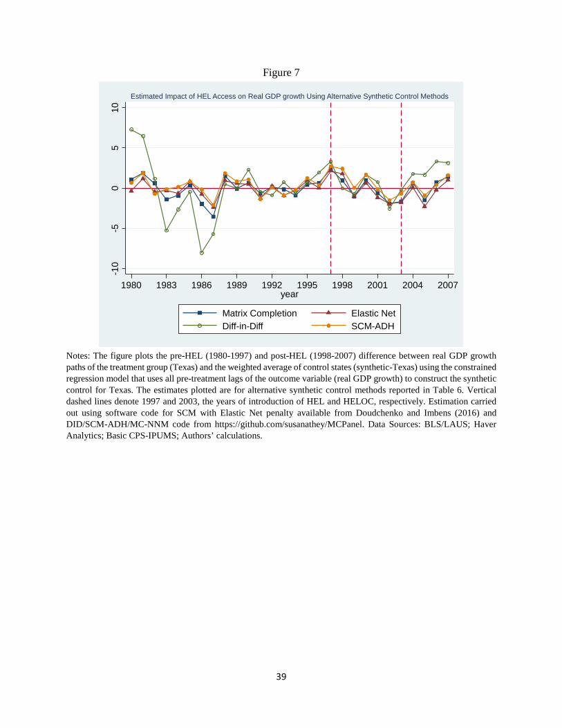
39

Figure 7

Notes: The figure plots the pre-HEL (1980-1997) and post-HEL (1998-2007) difference between real GDP growth paths of the treatment group (Texas) and the weighted average of control states (synthetic-Texas) using the constrained regression model that uses all pre-treatment lags of the outcome variable (real GDP growth) to construct the synthetic control for Texas. The estimates plotted are for alternative synthetic control methods reported in Table 6. Vertical dashed lines denote 1997 and 2003, the years of introduction of HEL and HELOC, respectively. Estimation carried out using software code for SCM with Elastic Net penalty available from Doudchenko and Imbens (2016) and DID/SCM-ADH/MC-NNM code from https://github.com/susanathey/MCPanel. Data Sources: BLS/LAUS; Haver Analytics; Basic CPS-IPUMS; Authors’ calculations.

-10

-50

510

1980 1983 1986 1989 1992 1995 1998 2001 2004 2007year

Matrix Completion Elastic NetDiff-in-Diff SCM-ADH

Estimated Impact of HEL Access on Real GDP growth Using Alternative Synthetic Control Methods

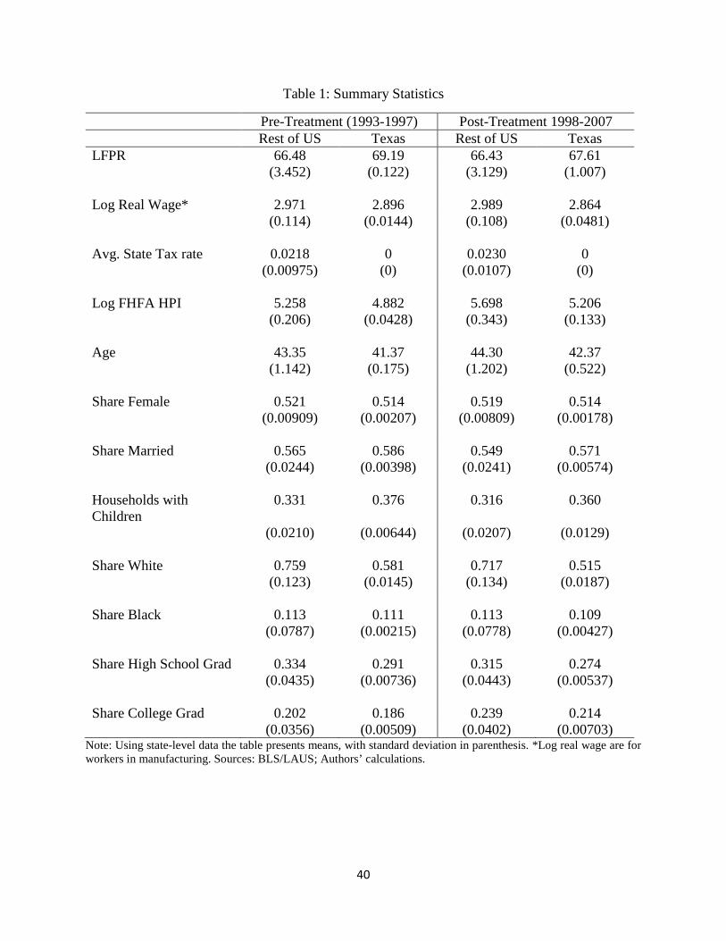
40

Table 1: Summary Statistics

Pre-Treatment (1993-1997) Post-Treatment 1998-2007 Rest of US Texas Rest of US Texas LFPR 66.48 69.19 66.43 67.61 (3.452) (0.122) (3.129) (1.007) Log Real Wage* 2.971 2.896 2.989 2.864 (0.114) (0.0144) (0.108) (0.0481) Avg. State Tax rate 0.0218 0 0.0230 0 (0.00975) (0) (0.0107) (0) Log FHFA HPI 5.258 4.882 5.698 5.206 (0.206) (0.0428) (0.343) (0.133) Age 43.35 41.37 44.30 42.37 (1.142) (0.175) (1.202) (0.522) Share Female 0.521 0.514 0.519 0.514 (0.00909) (0.00207) (0.00809) (0.00178) Share Married 0.565 0.586 0.549 0.571 (0.0244) (0.00398) (0.0241) (0.00574) Households with Children

0.331 0.376 0.316 0.360

(0.0210) (0.00644) (0.0207) (0.0129) Share White 0.759 0.581 0.717 0.515 (0.123) (0.0145) (0.134) (0.0187) Share Black 0.113 0.111 0.113 0.109 (0.0787) (0.00215) (0.0778) (0.00427) Share High School Grad 0.334 0.291 0.315 0.274 (0.0435) (0.00736) (0.0443) (0.00537) Share College Grad 0.202 0.186 0.239 0.214 (0.0356) (0.00509) (0.0402) (0.00703)

Note: Using state-level data the table presents means, with standard deviation in parenthesis. *Log real wage are for workers in manufacturing. Sources: BLS/LAUS; Authors’ calculations.

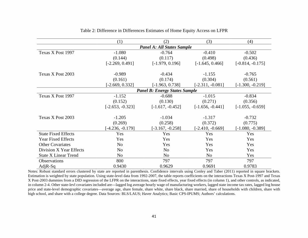
41

Table 2: Difference in Differences Estimates of Home Equity Access on LFPR

(1) (2) (3) (4) Panel A: All States Sample

Texas X Post 1997 -1.080 -0.764 -0.410 -0.502 (0.144) (0.117) (0.498) (0.436) [-2.269, 0.491] [-1.979, 0.196] [-1.645, 0.466] [-0.814, -0.175] Texas X Post 2003 -0.989 -0.434 -1.155 -0.765 (0.161) (0.174) (0.304) (0.561) [-2.669, 0.332] [-1.963, 0.738] [-2.311, -0.081] [-1.300, -0.219]

Panel B: Energy States Sample Texas X Post 1997 -1.152 -0.688 -1.015 -0.834 (0.152) (0.130) (0.271) (0.356) [-2.653, -0.323] [-1.617, -0.452] [-1.656, -0.441] [-1.055, -0.659] Texas X Post 2003 -1.205 -1.034 -1.317 -0.732 (0.269) (0.258) (0.372) (0.775) [-4.236, -0.179] [-3.167, -0.258] [-2.410, -0.669] [-1.080, -0.389] State Fixed Effects Yes Yes Yes Yes Year Fixed Effects Yes Yes Yes Yes Other Covariates No Yes Yes Yes Division X Year Effects No No Yes Yes State X Linear Trend No No No Yes Observations 800 797 797 797 AdjR-Sq 0.9430 0.9629 0.9691 0.9783

Notes: Robust standard errors clustered by state are reported in parenthesis. Confidence intervals using Conley and Taber (2011) reported in square brackets. Estimation is weighted by state population. Using state-level data from 1992-2007, the table reports coefficients on the interactions Texas X Post-1997 and Texas X Post-2003 dummies from a DID regression of the LFPR on the interactions, state fixed effects, year fixed effects (in column 1), and other controls, as indicated, in column 2-4. Other state-levl covariates included are—lagged log average hourly wage of manufacturing workers, lagged state income tax rates, lagged log house price and state-level demographic covariates—average age, share female, share white, share black, share married, share of households with children, share with high school, and share with a college degree. Data Sources: BLS/LAUS; Haver Analytics; Basic CPS-IPUMS; Authors’ calculations.

42

Table 3: Heterogeneity in Estimates of Home Equity Access on LFPR (1) (2) (3) (4) (5) (6) Male Female Prime-Age Age-55+ No-College Any-College Texas X Post 1997 -0.376 -0.639 -1.436 1.477 0.269 -1.886 (0.536) (0.802) (0.381) (0.890) (0.631) (0.745) [-1.748, 0.811] [-2.551, 1.347] [-3.522, -0.076] [-.658, 3.698] [-1.230, 1.979] [-3.970, -0.361] Texas X Post 2003 -0.789 -1.606 -0.383 -1.473 -1.565 -0.785 (0.442) (0.429) (0.403) (0.605) (0.673) (0.381) [-2.937, 0.488] [-3.713, -0.254] [-2.049, 0.919] [-.232, 1.570] [-3.764, 0.203] [-2.828, 0.478] State Fixed Effects Yes Yes Yes Yes Yes Yes Year Fixed Effects Yes Yes Yes Yes Yes Yes Demographic Controls Yes Yes Yes Yes Yes Yes Division X Year Effects Yes Yes Yes Yes Yes Yes Observations 63372 65417 48508 41464 67219 61570 AdjR-Sq 0.890 0.891 0.675 0.753 0.876 0.839 Notes: Robust standard errors clustered by state are reported in parenthesis. Confidence intervals using Conley and Taber (2011) reported in square brackets. Estimation is weighted by group-cell count. Using grouped basic CPS data by state, year and demographic groups from 1992-2007, the table reports coefficients on the interactions Texas X Post-1997 and Texas X Post-2003 dummies from a DID regression of the LFPR on the interactions, state fixed effects, year fixed effects, indicators for demographic groups as controls, and division X year effects. Data Sources: Basic Monthly CPS; Authors’ calculations.

43

Table 4: Synthetic Control Estimates with Standardized P-Values

Model with All Pre-Treatment

Lags

Model with

Covariates and Some

Lags

Model with All Pre-Treatment Lags:

Energy States

Model with All Pre-Treatment Lags:

Homeowners

Model with All Pre-Treatment Lags:

Renters

1998 -0.267 -0.527 -0.542 -1.354 0.337 [0.000] [0.163] [0.091] [0.082] [0.061] 1999 -0.545 -0.988 -1.032 -2.133 0.342 [0.000] [0.061] [0.091] [0.061] [0.061] 2000 -0.605 -1.566 -1.475 -1.383 -0.617 [0.000] [0.041] [0.091] [0.082] [0.082] 2001 -0.777 -1.804 -1.346 -2.061 2.598 [0.000] [0.082] [0.091] [0.061] [0.020] 2002 -0.565 -1.146 -0.569 -0.180 1.906 [0.000] [0.122] [0.091] [0.143] [0.020] 2003 -0.496 -1.181 -0.618 -1.267 0.879 [0.000] [0.163] [0.091] [0.082] [0.020] 2004 -0.869 -1.444 -1.003 -1.103 -0.935 [0.000] [0.061] [0.091] [0.102] [0.061] 2005 -1.459 -1.923 -1.477 -1.508 -3.320 [0.000] [0.041] [0.091] [0.102] [0.000] 2006 -1.985 -2.240 -1.816 -1.655 -2.865 [0.000] [0.020] [0.091] [0.082] [0.020]

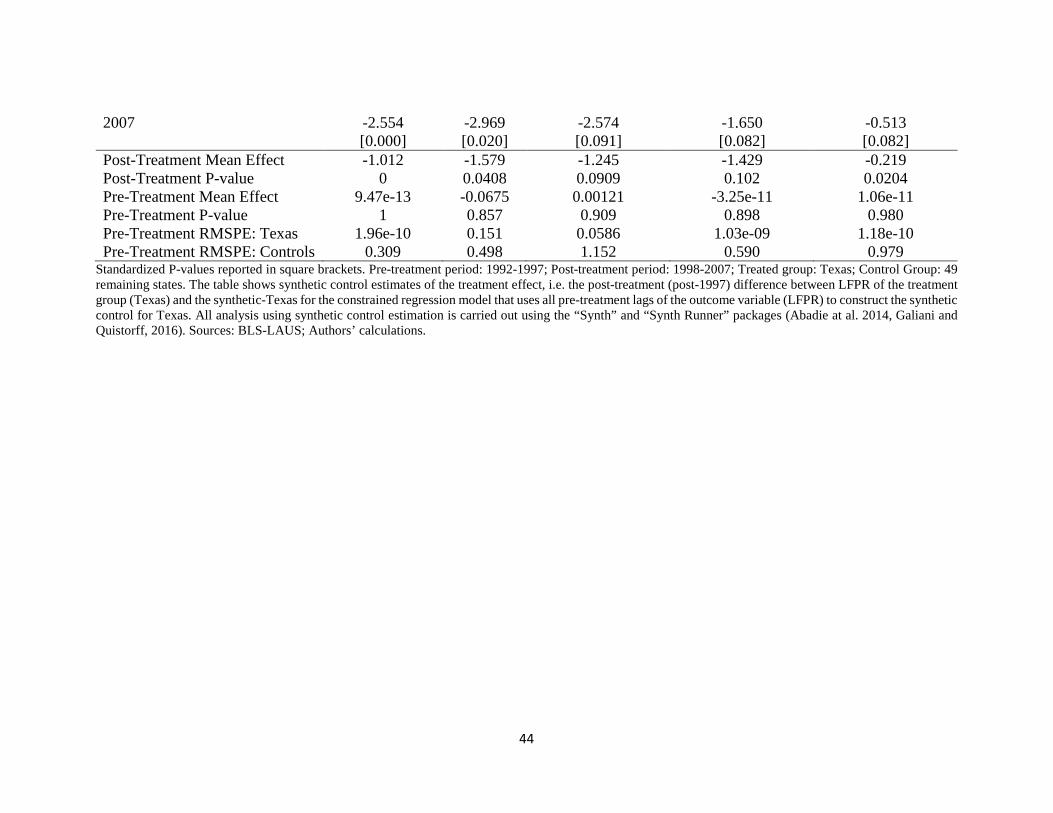
44

2007 -2.554 -2.969 -2.574 -1.650 -0.513 [0.000] [0.020] [0.091] [0.082] [0.082] Post-Treatment Mean Effect -1.012 -1.579 -1.245 -1.429 -0.219 Post-Treatment P-value 0 0.0408 0.0909 0.102 0.0204 Pre-Treatment Mean Effect 9.47e-13 -0.0675 0.00121 -3.25e-11 1.06e-11 Pre-Treatment P-value 1 0.857 0.909 0.898 0.980 Pre-Treatment RMSPE: Texas 1.96e-10 0.151 0.0586 1.03e-09 1.18e-10 Pre-Treatment RMSPE: Controls 0.309 0.498 1.152 0.590 0.979

Standardized P-values reported in square brackets. Pre-treatment period: 1992-1997; Post-treatment period: 1998-2007; Treated group: Texas; Control Group: 49 remaining states. The table shows synthetic control estimates of the treatment effect, i.e. the post-treatment (post-1997) difference between LFPR of the treatment group (Texas) and the synthetic-Texas for the constrained regression model that uses all pre-treatment lags of the outcome variable (LFPR) to construct the synthetic control for Texas. All analysis using synthetic control estimation is carried out using the “Synth” and “Synth Runner” packages (Abadie at al. 2014, Galiani and Quistorff, 2016). Sources: BLS-LAUS; Authors’ calculations.

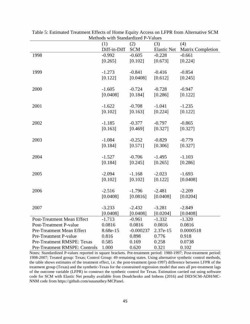
45

Table 5: Estimated Treatment Effects of Home Equity Access on LFPR from Alternative SCM Methods with Standardized P-Values

(1) (2) (3) (4) Diff-in-Diff SCM Elastic Net Matrix Completion 1998 -0.992 -0.605 -0.228 -0.661 [0.265] [0.102] [0.673] [0.224] 1999 -1.273 -0.841 -0.416 -0.854 [0.122] [0.0408] [0.612] [0.245] 2000 -1.605 -0.724 -0.728 -0.947 [0.0408] [0.184] [0.286] [0.122] 2001 -1.622 -0.708 -1.041 -1.235 [0.102] [0.163] [0.224] [0.122] 2002 -1.185 -0.377 -0.797 -0.865 [0.163] [0.469] [0.327] [0.327] 2003 -1.084 -0.252 -0.829 -0.779 [0.184] [0.571] [0.306] [0.327] 2004 -1.527 -0.706 -1.495 -1.103 [0.184] [0.245] [0.265] [0.286] 2005 -2.094 -1.168 -2.023 -1.693 [0.102] [0.102] [0.122] [0.0408] 2006 -2.516 -1.796 -2.481 -2.209 [0.0408] [0.0816] [0.0408] [0.0204] 2007 -3.233 -2.432 -3.281 -2.849 [0.0408] [0.0408] [0.0204] [0.0408] Post-Treatment Mean Effect -1.713 -0.961 -1.332 -1.320 Post-Treatment P-value 0.0816 0.0816 0.0816 0.0816 Pre-Treatment Mean Effect 8.68e-15 -0.000237 2.37e-15 0.0000518 Pre-Treatment P-value 0.816 0.898 0.776 0.918 Pre-Treatment RMSPE: Texas 0.585 0.169 0.258 0.0738 Pre-Treatment RMSPE: Controls 1.000 0.620 0.321 0.102

Notes: Standardized P-values reported in square brackets. Pre-treatment period: 1980-1997; Post-treatment period: 1998-2007; Treated group: Texas; Control Group: 49 remaining states. Using alternative synthetic control methods, the table shows estimates of the treatment effect, i.e. the post-treatment (post-1997) difference between LFPR of the treatment group (Texas) and the synthetic-Texas for the constrained regression model that uses all pre-treatment lags of the outcome variable (LFPR) to construct the synthetic control for Texas. Estimation carried out using software code for SCM with Elastic Net penalty available from Doudchenko and Imbens (2016) and DID/SCM-ADH/MC-NNM code from https://github.com/susanathey/MCPanel.

46

Table 6: Estimated Treatment Effects of Home Equity Access on Real GDP Growth with Standardized P-Values

(1) (2) (3) (4) Diff-in-Diff SCM Elastic Net Matrix Completion 1998 -0.0213 2.414 1.783 0.950 [1] [0.184] [0.429] [0.633] 1999 -0.734 0.0385 -1.024 -1.010 [0.714] [0.959] [0.490] [0.551] 2000 1.699 1.651 0.630 0.986 [0.571] [0.388] [0.755] [0.694] 2001 0.717 -0.148 -1.179 -0.623 [0.898] [0.918] [0.429] [0.857] 2002 -2.562 -1.502 -1.938 -1.935 [0.306] [0.408] [0.245] [0.224] 2003 -0.243 -0.685 -1.758 -1.662 [0.980] [0.571] [0.224] [0.388] 2004 1.771 0.713 0.0606 0.625 [0.612] [0.735] [0.959] [0.735] 2005 1.646 -0.922 -2.279 -1.485 [0.735] [0.694] [0.306] [0.490] 2006 3.339 0.399 -0.211 0.711 [0.429] [0.694] [0.918] [0.653] 2007 3.111 1.616 1.009 1.403 [0.510] [0.490] [0.612] [0.592] Post-Treatment Mean Effect 0.872 0.357 -0.491 -0.204 Post-Treatment P-value 0.959 0.837 0.837 0.959 Pre-Treatment Mean Effect 1.17e-16 0.337 3.70e-17 0.00304 Pre-Treatment P-value 0.143 0.429 0.429 0.367 Pre-Treatment RMSPE: Texas 3.741 1.218 1.017 1.386 Pre-Treatment RMSPE: Controls 2.980 1.541 1.119 1.328

Notes: Standardized P-values reported in square brackets. Pre-treatment period: 1980-1997; Post-treatment period: 1998-2007; Treated group: Texas; Control Group: 49 remaining states. Using alternative synthetic control methods, the table shows estimates of the treatment effect, i.e. the post-treatment (post-1997) difference between LFPR of the treatment group (Texas) and the synthetic-Texas for the constrained regression model that uses all pre-treatment lags of the outcome variable (real GDP growth) to construct the synthetic control for Texas. Estimation carried out using software code for SCM with Elastic Net penalty available from Doudchenko and Imbens (2016) and DID/SCM-ADH/MC-NNM code from https://github.com/susanathey/MCPanel.

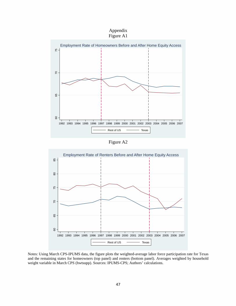
47

Appendix Figure A1

Figure A2

Notes: Using March CPS-IPUMS data, the figure plots the weighted-average labor force participation rate for Texas and the remaining states for homeowners (top panel) and renters (bottom panel). Averages weighted by household weight variable in March CPS (hwtsupp). Sources: IPUMS-CPS; Authors’ calculations.

6065

7075

1992 1993 1994 1995 1996 1997 1998 1999 2000 2001 2002 2003 2004 2005 2006 2007

Rest of US Texas

Employment Rate of Homeowners Before and After Home Equity Access

6065

7075

8085

1992 1993 1994 1995 1996 1997 1998 1999 2000 2001 2002 2003 2004 2005 2006 2007

Rest of US Texas

Employment Rate of Renters Before and After Home Equity Access

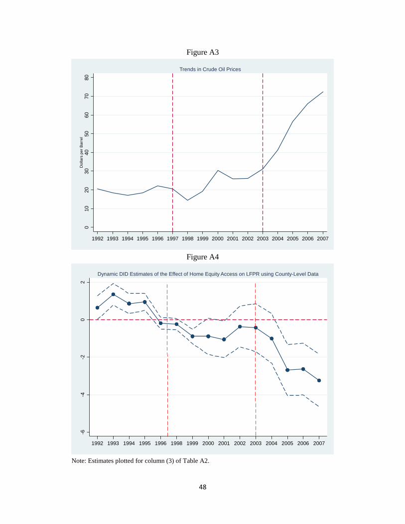
48

Figure A3

Figure A4

Note: Estimates plotted for column (3) of Table A2.

010

2030

4050

6070

80D

olla

rs p

er B

arre

l

1992 1993 1994 1995 1996 1997 1998 1999 2000 2001 2002 2003 2004 2005 2006 2007

Trends in Crude Oil Prices

-6-4

-20

2

1992 1993 1994 1995 1996 1998 1999 2000 2001 2002 2003 2004 2005 2006 2007

Dynamic DID Estimates of the Effect of Home Equity Access on LFPR using County-Level Data

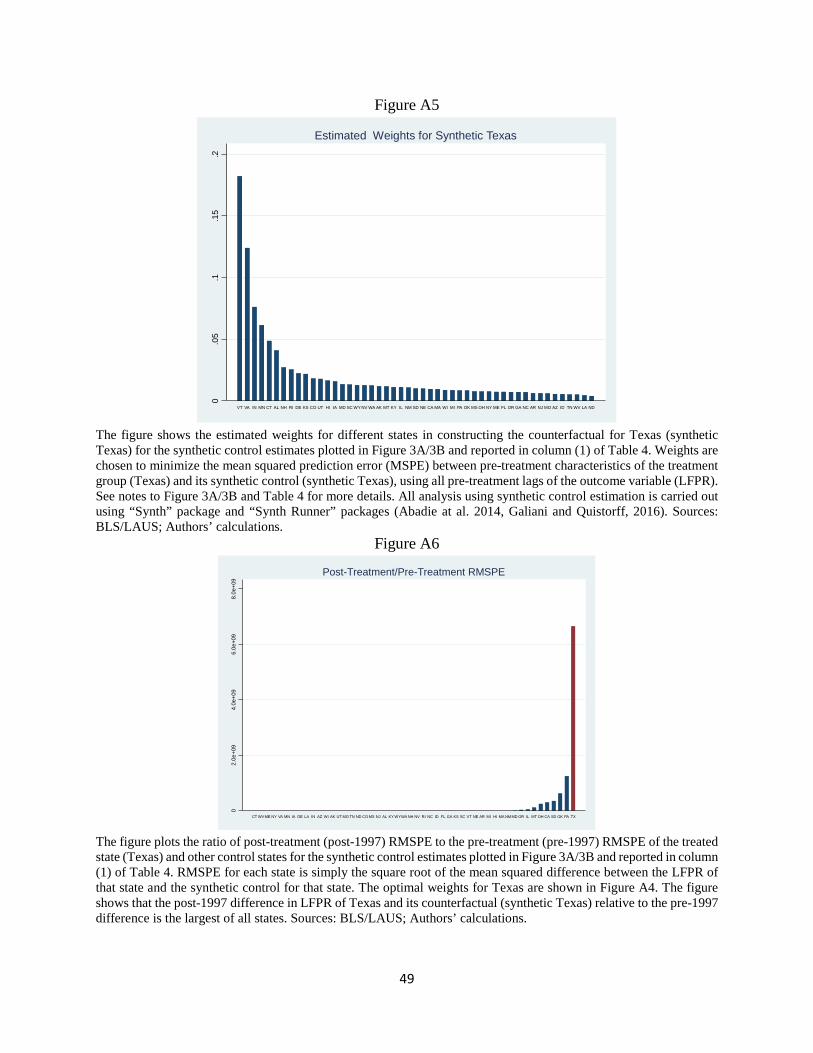
49

Figure A5

The figure shows the estimated weights for different states in constructing the counterfactual for Texas (synthetic Texas) for the synthetic control estimates plotted in Figure 3A/3B and reported in column (1) of Table 4. Weights are chosen to minimize the mean squared prediction error (MSPE) between pre-treatment characteristics of the treatment group (Texas) and its synthetic control (synthetic Texas), using all pre-treatment lags of the outcome variable (LFPR). See notes to Figure 3A/3B and Table 4 for more details. All analysis using synthetic control estimation is carried out using “Synth” package and “Synth Runner” packages (Abadie at al. 2014, Galiani and Quistorff, 2016). Sources: BLS/LAUS; Authors’ calculations.

Figure A6

The figure plots the ratio of post-treatment (post-1997) RMSPE to the pre-treatment (pre-1997) RMSPE of the treated state (Texas) and other control states for the synthetic control estimates plotted in Figure 3A/3B and reported in column (1) of Table 4. RMSPE for each state is simply the square root of the mean squared difference between the LFPR of that state and the synthetic control for that state. The optimal weights for Texas are shown in Figure A4. The figure shows that the post-1997 difference in LFPR of Texas and its counterfactual (synthetic Texas) relative to the pre-1997 difference is the largest of all states. Sources: BLS/LAUS; Authors’ calculations.

0.0

5.1

.15

.2

VT VA IN MN CT AL NH RI DE KS CO UT HI IA MD SC WY NV WA AK MT KY IL NM SD NE CA MA WI MI PA OK MS OH NY ME FL OR GA NC AR NJ MO AZ ID TN WV LA ND

Estimated Weights for Synthetic Texas

02.

0e+0

94.

0e+0

96.

0e+0

98.

0e+0

9

CT WVME NY VA MN IA DE LA IN AZ WI AK UT MO TN ND CO MS NJ AL KY WYWA NH NV RI NC ID FL GA KS SC VT NE AR MI HI MA NMMD OR IL MT OH CA SD OK PA TX

Post-Treatment/Pre-Treatment RMSPE

50

Figure A7

The figure shows the estimated weights for different states in constructing the counterfactual for Texas (synthetic Texas) for the synthetic control estimates plotted in Figure 4A/4B. The figure is analogous to Figure A4, except that it plots estimated weights for SCM-ADH estimated effects of HELOC in the post-2003 period. See notes to Figure A4 for more details.

Figure A8

The figure plots the ratio of post-HELOC (2004-2007) RMSPE to the pre-HELOC (1998-2003) RMSPE of the treatment state (Texas) vs. other states for the synthetic control estimates plotted in Figure 4A/4B. The figure is analogous to Figure A6, except that it uses SCM-ADH estimates of HELOC in the post-2003 period. See notes to Figure A6 for more details.

0.0

5.1

.15

.2

CO NM IA KS AR MS IN NY ND NJ RI CT MA MD VA CA GA TN OR VT OH MOWA SC PA AL MT OK AZ SD WI ME UT LA ID FL NC KY NE DE NH WV HI NV WY MI IL AK MN

Estimated Weights for Synthetic Texas (1998-2003)

01.

0e+0

92.

0e+0

93.

0e+0

94.

0e+0

95.

0e+0

9

MNWYSC VT WVNMWA DE ID SD KS CO IA MS PA ME AZ NE AK IL NV HI WI LA MO MI VA KY AR RI NC ND NY OR MD TN CA MA AL CT FL MT GA NJ OK IN OH NH UT TX

Post-Treatment/Pre-Treatment RMSPE for SCM Estimates of the Effect of HELOC

51

Figure A9

Figure A10

6667

6869

70

1992 1993 1994 1995 1996 1997 1998 1999 2000 2001 2002 2003 2004 2005 2006 2007

TX synthetic TX

LFPR in Texas vs. Synthetic Texas Before and After Home equity Access with Some Lags and Covariates-4

-20

24

6

1992 1995 1998 2001 2004 2007

Synthetic Control Estimates of the Effect of Home Equity Access on LFPR in Texas vs. Placebo States

52

Figure A11

Using grouped March CPS-IPUMS data for homeowners and renters, the figure plots the difference between LFPR paths of Texas and synthetic Texas for the constrained regression model that uses all pre-treatment lags of the outcome variable (LFPR) to construct the synthetic control for Texas. The figure shows that the pre-treatment path of LFPR of “synthetic Texas” is almost identical to that for Texas for both homeowners and renters, yet the post-treatment paths diverge significantly for homeowners and there is no clear trend for renters. The post-HEL mean effect is large for homeowners and relatively very small for renters. All analysis using synthetic control estimation is carried out using “Synth” package and “Synth Runner” packages Abadie at al. (2014), Galiani and Quistorff (2016). Data Sources: March CPS-IPUMS; Authors’ calculations.

-4-2

02

4G

ap in

LFP

R (T

X m

inus

Syn

thet

ic T

X)

1992 1995 1998 2001 2004 2007

Homeowners Post-HEL Mean Effect

Renters Post-HEL Mean Effect

SCM Estimates of the Effect on Employment Rate by Homeownership

53

Figure A12

Figure A13

-10

-50

5

1980 1983 1986 1989 1992 1995 1998 2001 2004 2007year

Estimates of the Effect of HEL Access on LFPR in Texas vs. Placebo States using SCM-4

-20

24

6

1980 1983 1986 1989 1992 1995 1998 2001 2004 2007

SCM Estimates of the Effect of HEL Access on LFPR in Texas vs. Placebo States using Elasticnet

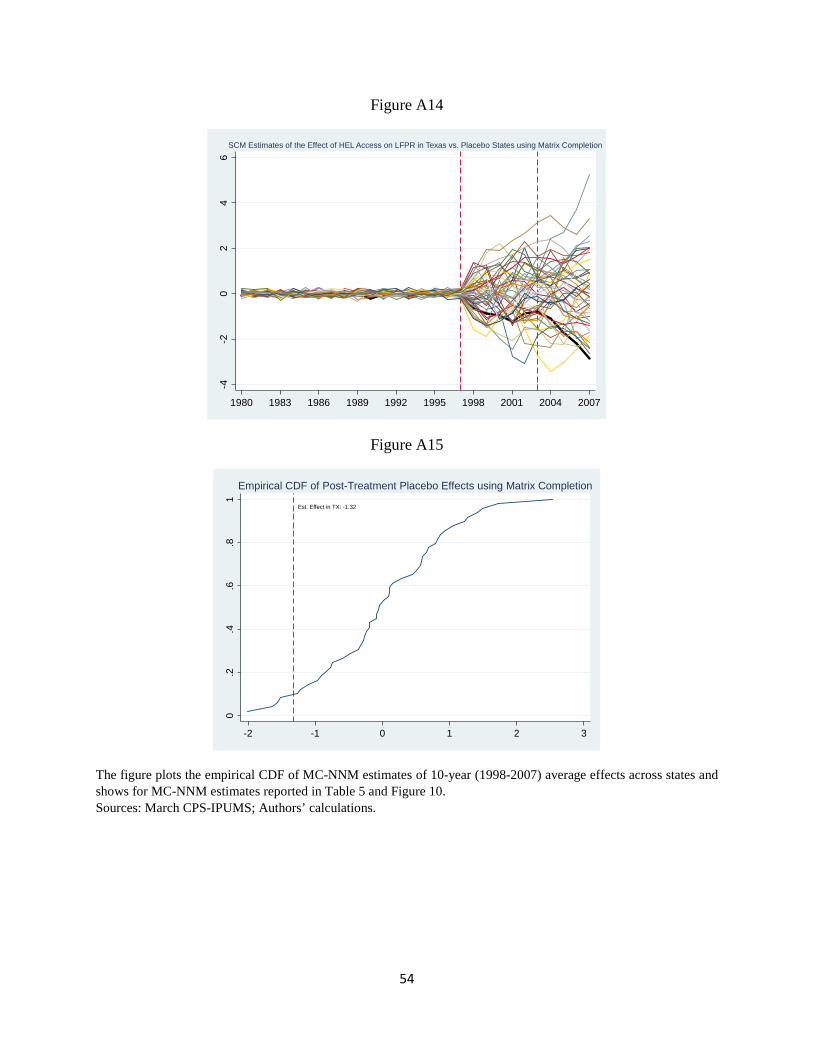
54

Figure A14

Figure A15

The figure plots the empirical CDF of MC-NNM estimates of 10-year (1998-2007) average effects across states and shows for MC-NNM estimates reported in Table 5 and Figure 10. Sources: March CPS-IPUMS; Authors’ calculations.

-4-2

02

46

1980 1983 1986 1989 1992 1995 1998 2001 2004 2007

SCM Estimates of the Effect of HEL Access on LFPR in Texas vs. Placebo States using Matrix Completion

Est. Effect in TX: -1.32

0.2

.4.6

.81

-2 -1 0 1 2 3

Empirical CDF of Post-Treatment Placebo Effects using Matrix Completion

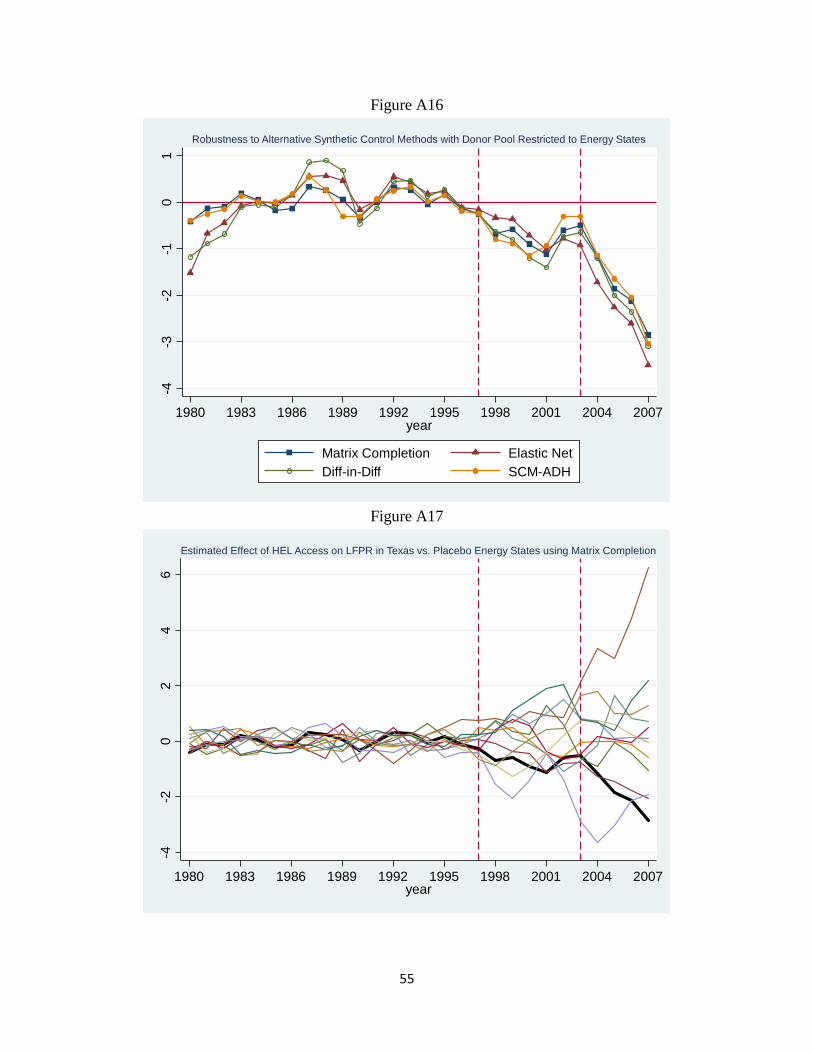
55

Figure A16

Figure A17

-4-3

-2-1

01

1980 1983 1986 1989 1992 1995 1998 2001 2004 2007year

Matrix Completion Elastic NetDiff-in-Diff SCM-ADH

Robustness to Alternative Synthetic Control Methods with Donor Pool Restricted to Energy States

-4-2

02

46

1980 1983 1986 1989 1992 1995 1998 2001 2004 2007year

Estimated Effect of HEL Access on LFPR in Texas vs. Placebo Energy States using Matrix Completion

56

Table A1: Time-varying Difference in Differences Estimates of Home Equity Access on LFPR using State-Level Data

(1) (2) (3) (4) 1992 0.63127 0.64802 -0.38987 (0.229) (0.159) (0.732) 1993 0.80334 0.69861 0.43466 (0.175) (0.142) (0.612) 1994 0.76639 0.65835 0.21006 (0.181) (0.152) (0.574) 1995 0.71015 0.72102 0.21365 (0.186) (0.169) (0.617) 1996 0.29280 0.17418 -0.19346 (0.111) (0.121) (0.354) 1998 -0.16751 -0.36178 -0.19037 -0.25411 (0.079) (0.107) (0.317) (0.494) 1999 -0.48739 -0.46684 -0.47751 -0.29827 (0.118) (0.098) (0.164) (0.418) 2000 -0.91417 -1.00487 -1.00895 -0.47769 (0.180) (0.163) (0.238) (0.492) 2001 -0.94969 -0.52108 -0.72776 -0.13961 (0.213) (0.156) (0.207) (0.471) 2002 -0.51978 -0.02806 -0.39678 0.27748 (0.214) (0.175) (0.168) (0.498) 2003 -0.27963 0.47036 0.66696 1.58027 (0.177) (0.181) (0.283) (0.705) 2004 -0.70975 -0.09650 -0.31473 0.73083 (0.195) (0.211) (0.206) (0.721) 2005 -1.23453 -0.51133 -1.75868 -0.47843 (0.218) (0.222) (0.419) (1.272) 2006 -1.68231 -0.92287 -1.77997 -0.32344 (0.227) (0.228) (0.629) (1.425)

57

2007 -2.48743 -1.42771 -2.10719 -0.30547 (0.269) (0.283) (0.414) (1.321) State Fixed Effects Yes Yes Yes Yes Year Fixed Effects Yes Yes Yes Yes Wage, Tax Rate, House Price No Yes Yes Yes Demographic Controls No Yes Yes Yes Division X Year Effects No No Yes Yes State X Linear Trend No No No Yes Observations 800 797 797 797 AdjR-Sq 0.9434 0.9635 0.9693 0.9788

Notes: Robust standard errors clustered by state are reported in parenthesis. Estimation is weighted by state population. Using state-level data from 1992-2007, the table reports coefficients on the interactions between the treatment dummy (an indicator for Texas) and dummies for each year from 1992 to 2007 from a regression of the LFPR on Texas X Year interactions, state effects, year effects (in column 1), and other controls, as indicated, in column 2-4. 1997 is the omitted base year, with its interaction with the treatment dummy normalized to zero, so that estimates should be interpreted as the difference between Texas and rest of U.S. relative to the difference in year 1997—the year just before the law change. See notes to Table 2 for details on additional covariates included in columns 2-4. Pre-treatment interactions are excluded in column 4 to identify state-specific linear time trends. Sources: BLS-LAUS; Authors’ calculations.

58

Table A2: Time-varying Difference in Differences Estimates of Home Equity Access on LFPR using County-Level Data

(1) (2) (3) (4) 1992 1.49834 1.40140 0.64306 (0.298) (0.310) (0.383) 1993 1.41529 1.28691 1.35349 (0.256) (0.267) (0.353) 1994 1.50619 1.34538 0.86031 (0.203) (0.211) (0.323) 1995 1.36632 1.23068 0.94277 (0.160) (0.166) (0.275) 1996 0.55892 0.47353 -0.18982 (0.122) (0.119) (0.192) 1998 0.35756 0.32645 -0.23817 -0.03937 (0.133) (0.144) (0.180) (0.256) 1999 -0.20908 -0.27384 -0.89012 -0.45954 (0.154) (0.166) (0.234) (0.305) 2000 -1.54467 -1.69093 -0.89118 -0.23172 (0.503) (0.511) (0.590) (0.621) 2001 -1.56809 -1.73809 -1.05306 -0.16359 (0.490) (0.493) (0.592) (0.678) 2002 -0.83465 -0.99346 -0.36736 0.75115 (0.529) (0.532) (0.660) (0.797) 2003 -0.58730 -0.77286 -0.42593 0.92125 (0.661) (0.655) (0.777) (0.953) 2004 -0.92318 -1.04746 -1.00133 0.57404 (0.694) (0.690) (0.804) (1.024) 2005 -1.63405 -1.60630 -2.69430 -0.89124 (0.693) (0.694) (0.827) (1.093) 2006 -2.48710 -2.33464 -2.64006 -0.60960 (0.679) (0.674) (0.839) (1.165)

59

2007 -3.13346 -2.96846 -3.24586 -0.98695 (0.671) (0.661) (0.856) (1.271) County Fixed Effects Yes Yes Yes Yes Year Fixed Effects Yes Yes Yes Yes House Price No Yes Yes Yes Division X Year Effects No No Yes Yes State X Linear Trend No No No Yes Observations 46672 33717 33717 33717 AdjR-Sq 0.8873 0.8931 0.9017 0.9069

Notes: Robust standard errors clustered by county are reported in parenthesis. Estimation is weighted by county population. Using county-level data from 1992-2007, the table reports coefficients on the interactions between the treatment dummy (an indicator for Texas) and dummies for each year from 1992 to 2007 from a regression of the LFPR on Texas X Year interactions, state effects, year effects (in column 1), and other controls, as indicated, in column 2-4. 1997 is the omitted base year, with its interaction with the treatment dummy normalized to zero, so that estimates should be interpreted as the difference between Texas and rest of U.S. relative to the difference in year 1997—the year just before the law change. Pre-treatment interactions are excluded in column 4 to identify state-specific linear time trends. Sources: BLS-LAUS; Authors’ calculations.

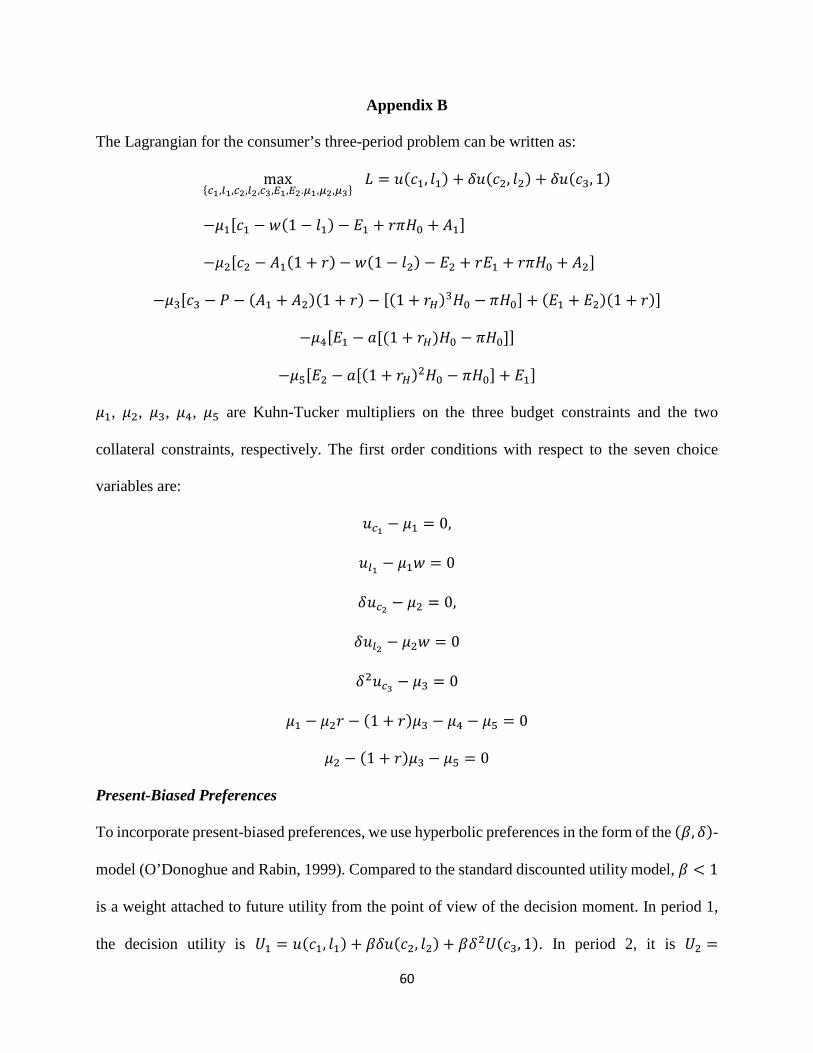
60

Appendix B

The Lagrangian for the consumer’s three-period problem can be written as:

max{𝑐𝑐1,𝑙𝑙1,𝑐𝑐2,𝑙𝑙2,𝑐𝑐3,𝐻𝐻1,𝐻𝐻2.𝜇𝜇1,𝜇𝜇2,𝜇𝜇3}

𝐿𝐿 = 𝑢𝑢(𝑐𝑐1, 𝑙𝑙1) + 𝛿𝛿𝑢𝑢(𝑐𝑐2, 𝑙𝑙2) + 𝛿𝛿𝑢𝑢(𝑐𝑐3, 1)

−𝜇𝜇1[𝑐𝑐1 − 𝑤𝑤(1 − 𝑙𝑙1) − 𝐸𝐸1 + 𝑟𝑟𝑟𝑟𝐻𝐻0 + 𝐴𝐴1]

−𝜇𝜇2[𝑐𝑐2 − 𝐴𝐴1(1 + 𝑟𝑟) − 𝑤𝑤(1 − 𝑙𝑙2) − 𝐸𝐸2 + 𝑟𝑟𝐸𝐸1 + 𝑟𝑟𝑟𝑟𝐻𝐻0 + 𝐴𝐴2]

−𝜇𝜇3[𝑐𝑐3 − 𝑃𝑃 − (𝐴𝐴1 + 𝐴𝐴2)(1 + 𝑟𝑟) − [(1 + 𝑟𝑟𝐻𝐻)3𝐻𝐻0 − 𝑟𝑟𝐻𝐻0] + (𝐸𝐸1 + 𝐸𝐸2)(1 + 𝑟𝑟)]

−𝜇𝜇4[𝐸𝐸1 − 𝑎𝑎[(1 + 𝑟𝑟𝐻𝐻)𝐻𝐻0 − 𝑟𝑟𝐻𝐻0]]

−𝜇𝜇5[𝐸𝐸2 − 𝑎𝑎[(1 + 𝑟𝑟𝐻𝐻)2𝐻𝐻0 − 𝑟𝑟𝐻𝐻0] + 𝐸𝐸1]

𝜇𝜇1, 𝜇𝜇2, 𝜇𝜇3, 𝜇𝜇4, 𝜇𝜇5 are Kuhn-Tucker multipliers on the three budget constraints and the two

collateral constraints, respectively. The first order conditions with respect to the seven choice

variables are:

𝑢𝑢𝑐𝑐1 − 𝜇𝜇1 = 0,

𝑢𝑢𝑙𝑙1 − 𝜇𝜇1𝑤𝑤 = 0

𝛿𝛿𝑢𝑢𝑐𝑐2 − 𝜇𝜇2 = 0,

𝛿𝛿𝑢𝑢𝑙𝑙2 − 𝜇𝜇2𝑤𝑤 = 0

𝛿𝛿2𝑢𝑢𝑐𝑐3 − 𝜇𝜇3 = 0

𝜇𝜇1 − 𝜇𝜇2𝑟𝑟 − (1 + 𝑟𝑟)𝜇𝜇3 − 𝜇𝜇4 − 𝜇𝜇5 = 0

𝜇𝜇2 − (1 + 𝑟𝑟)𝜇𝜇3 − 𝜇𝜇5 = 0

Present-Biased Preferences

To incorporate present-biased preferences, we use hyperbolic preferences in the form of the (𝛽𝛽, 𝛿𝛿)-

model (O’Donoghue and Rabin, 1999). Compared to the standard discounted utility model, 𝛽𝛽 < 1

is a weight attached to future utility from the point of view of the decision moment. In period 1,

the decision utility is 𝑈𝑈1 = 𝑢𝑢(𝑐𝑐1, 𝑙𝑙1) + 𝛽𝛽𝛿𝛿𝑢𝑢(𝑐𝑐2, 𝑙𝑙2) + 𝛽𝛽𝛿𝛿2𝑈𝑈(𝑐𝑐3, 1). In period 2, it is 𝑈𝑈2 =

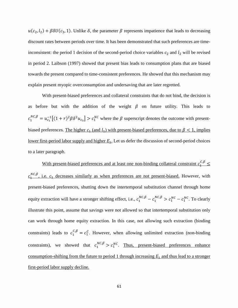
61

𝑢𝑢(𝑐𝑐2, 𝑙𝑙2) + 𝛽𝛽𝛿𝛿𝑈𝑈(𝑐𝑐3, 1). Unlike 𝛿𝛿, the parameter 𝛽𝛽 represents impatience that leads to decreasing

discount rates between periods over time. It has been demonstrated that such preferences are time-

inconsistent: the period 1 decision of the second-period choice variables 𝑐𝑐2 and 𝑙𝑙2 will be revised

in period 2. Laibson (1997) showed that present bias leads to consumption plans that are biased

towards the present compared to time-consistent preferences. He showed that this mechanism may

explain present myopic overconsumption and undersaving that are later regretted.

With present-biased preferences and collateral constraints that do not bind, the decision is

as before but with the addition of the weight 𝛽𝛽 on future utility. This leads to

𝑐𝑐1𝑁𝑁𝑁𝑁,𝛽𝛽 = 𝑢𝑢𝑐𝑐1

−1�(1 + 𝑟𝑟)2𝛽𝛽𝛿𝛿2𝑢𝑢𝑐𝑐3� > 𝑐𝑐1𝑁𝑁𝑁𝑁 where the 𝛽𝛽 superscript denotes the outcome with present-

biased preferences. The higher 𝑐𝑐1 (and 𝑙𝑙1) with present-biased preferences, due to 𝛽𝛽 < 1, implies

lower first-period labor supply and higher 𝐸𝐸1. Let us defer the discussion of second-period choices

to a later paragraph.

With present-biased preferences and at least one non-binding collateral constraint 𝑐𝑐1𝑁𝑁,𝛽𝛽 ≤

𝑐𝑐1𝑁𝑁𝑁𝑁,𝛽𝛽, i.e. 𝑐𝑐1 decreases similarly as when preferences are not present-biased. However, with

present-biased preferences, shutting down the intertemporal substitution channel through home

equity extraction will have a stronger shifting effect, i.e., 𝑐𝑐1𝑁𝑁𝑁𝑁,𝛽𝛽 − 𝑐𝑐1

𝑁𝑁𝑁𝑁,𝛽𝛽 > 𝑐𝑐1𝑁𝑁𝑁𝑁 − 𝑐𝑐1𝑁𝑁𝑁𝑁. To clearly

illustrate this point, assume that savings were not allowed so that intertemporal substitution only

can work through home equity extraction. In this case, not allowing such extraction (binding

constraints) leads to 𝑐𝑐1𝑁𝑁,𝛽𝛽 = 𝑐𝑐1𝑁𝑁 . However, when allowing unlimited extraction (non-binding

constraints), we showed that 𝑐𝑐1𝑁𝑁𝑁𝑁,𝛽𝛽 > 𝑐𝑐1𝑁𝑁𝑁𝑁. Thus, present-biased preferences enhance

consumption-shifting from the future to period 1 through increasing 𝐸𝐸1 and thus lead to a stronger

first-period labor supply decline.

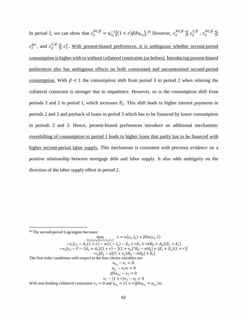
62

In period 2, we can show that 𝑐𝑐2𝑁𝑁𝑁𝑁,𝛽𝛽 = 𝑢𝑢𝑐𝑐2

−1�(1 + 𝑟𝑟)𝛽𝛽𝛿𝛿𝑢𝑢𝑐𝑐3�.20 However, 𝑐𝑐2

𝑁𝑁𝑁𝑁,𝛽𝛽 ⋚ 𝑐𝑐2𝑁𝑁,𝛽𝛽 , 𝑐𝑐2

𝑁𝑁𝑁𝑁,𝛽𝛽 ⋚

𝑐𝑐2𝑁𝑁𝑁𝑁, and 𝑐𝑐2𝑁𝑁,𝛽𝛽 ⋚ 𝑐𝑐2𝑁𝑁. With present-biased preferences, it is ambiguous whether second-period

consumption is higher with or without collateral constraints (as before). Introducing present-biased

preferences also has ambiguous effects on both constrained and unconstrained second-period

consumption. With 𝛽𝛽 < 1 the consumption shift from period 3 to period 2 when relaxing the

collateral constraint is stronger due to impatience. However, so is the consumption shift from

periods 3 and 2 to period 1, which increases 𝐸𝐸1. This shift leads to higher interest payments in

periods 2 and 3 and payback of loans in period 3 which has to be financed by lower consumption

in periods 2 and 3. Hence, present-biased preferences introduce an additional mechanism:

overshifting of consumption to period 1 leads to higher loans that partly has to be financed with

higher second-period labor supply. This mechanism is consistent with previous evidence on a

positive relationship between mortgage debt and labor supply. It also adds ambiguity on the

direction of the labor supply effect in period 2.

20 The second-period Lagrangian becomes:

max{𝑐𝑐2,𝑙𝑙2,𝑐𝑐3,𝐻𝐻2,𝜈𝜈1,𝜈𝜈2,𝜈𝜈3}

𝐿𝐿 = 𝑢𝑢(𝑐𝑐2, 𝑙𝑙2) + 𝛽𝛽𝛿𝛿𝑢𝑢(𝑐𝑐3, 1)

−𝜈𝜈1[𝑐𝑐2 − 𝐴𝐴1(1 + 𝑟𝑟) − 𝑤𝑤(1 − 𝑙𝑙2) − 𝐸𝐸2 + 𝑟𝑟𝐸𝐸1 + 𝑟𝑟𝑟𝑟𝐻𝐻0 + 𝐴𝐴2](𝐸𝐸1 + 𝐸𝐸2) −𝜈𝜈2[𝑐𝑐3 − 𝑃𝑃 − (𝐴𝐴1 + 𝐴𝐴2)(1 + 𝑟𝑟) − [(1 + 𝑟𝑟𝐻𝐻)3𝐻𝐻0 − 𝑟𝑟𝐻𝐻0] + (𝐸𝐸1 + 𝐸𝐸2)(1 + 𝑟𝑟)]

−𝜈𝜈3[𝐸𝐸2 − 𝑎𝑎[(1 + 𝑟𝑟𝐻𝐻)𝐻𝐻0 − 𝑟𝑟𝐻𝐻0] + 𝐸𝐸1] The first order conditions with respect to the four choice variables are:

𝑢𝑢𝑐𝑐2 − 𝜈𝜈1 = 0, 𝑢𝑢𝑙𝑙2 − 𝜈𝜈1𝑤𝑤 = 0 𝛽𝛽𝛿𝛿𝑢𝑢𝑐𝑐3 − 𝜈𝜈2 = 0

𝜈𝜈1 − (1 + 𝑟𝑟)𝜈𝜈2 − 𝜈𝜈3 = 0 With non-binding collateral constraints 𝜈𝜈3 = 0 and 𝑢𝑢𝑐𝑐2 = (1 + 𝑟𝑟)𝛽𝛽𝛿𝛿𝑢𝑢𝑐𝑐3 = 𝑢𝑢𝑙𝑙2 𝑤𝑤⁄ .