labor market and growth implications of emigration: cross...
TRANSCRIPT

BACKGROUND PAPER FOR THE
WORLD DEVELOPMENT REPORT 2013
Labor Market and Growth Implications of Emigration: Cross-Country Evidence
Shoghik Hovhannisyan The World Bank
Labor Market and Growth Implications of Emigration:
Cross-Country Evidence
Shoghik Hovhannisyan
Abstract
The number of migrants residing in 30 OECD countries increased from 42 million to nearly
59 million over 1990-2000. This paper studies the impact of emigrants with different education
levels on their home countries’ employment-population ratio, GDP per worker, and its factors
obtained by a production function decomposition. It uses migration data from 195 countries of
origin to 30 major destination OECD countries in 1990 and 2000 and applies two different econo-
metric approaches to estimate this impact. The first approach discusses how changes in native
population due to emigration affect the growth of macroeconomic variables and constructs an
instrument based on pull factors of migration and migrants’ networks to correct for endogene-
ity bias. The second approach estimates the elasticities of variables of interest with respect to
emigration rates and uses instruments widely discussed in the literature: dummy variables for
being in a colonial relationship; low-income countries; whether the migrant sending country’s
official language is English; distance; and country size. Estimation results across two economet-
ric approaches indicate that total emigration rates increase GDP per worker in all countries,
non-high income countries, and low and lower middle income countries, primarily driven by im-
provements in total factor productivity (TFP). In contrast, there is no robust significant impact
of emigration on the employment-population ratio across different specifications.
1

1 Introduction
Along with increased flows of capital, goods, and services, international labor mobility has become
an inseparable part of globalization, with enormous economic, social and cultural implications
in both countries of origin and destination. The number of foreign-born individuals residing in
30 OECD countries increased from 42 million to nearly 59 million over the period of 1990-2000.
This paper studies the impact of emigration for different education levels on GDP per worker, its
factors obtained by a production function decomposition, and the employment-population ratio in
migrant-sending countries. It uses data on emigration from 195 countries of origin to 30 OECD
destination countries which account for about 70 percent of total emigration and 90 percent of
skilled emigration in the world. Emigration can have both a negative and a positive impact on
migrant-sending countries. On one hand, these countries face deprivation of their labor force
especially the most educated, known in the literature as a brain drain phenomenon. On the other
hand they benefit from emigration in several ways. Migrants remit money home and these financial
flows account for a significant share of GDP in developing countries. Remittances relax financial
constraints of households which have a member or relative abroad and can increase not only their
consumption of goods and services, but also expenditures on health and education, thus having both
short-term and long-term effects on GDP. Emigration might also promote transfer of technology
and knowledge across countries by facilitating more foreign direct investment (FDI), trade, and
other partnerships through established diasporas abroad and their networks. Finally, the high
probability of emigration of educated labor raises returns to education and, therefore, might lead
to higher investments in education. As not everyone has a chance to migrate, this increases overall
human capital in the migrant-sending country.
There is a large empirical literature on emigration effects in migrant-sending countries and their
various transmission mechanisms. Macroeconomic studies using cross-country data provide mixed
evidence on the effects of emigration and remittances on growth and its drivers, with results highly
dependent on the econometric approaches and instruments used to control for endogeneity bias.
Estimations by Cartinescu et al. (2009) and Acosta et al. (2008) show an increase in growth due
to remittances, while Chami et al. (2009) find a negative effect of remittances on growth volatility.
However, Barajas et al. (2009) conclude that remittances have no impact on economic growth
2

in their cross-country analysis. At the same time, Easterly and Nyarko (2009) find no significant
impact of brain drain or outflow of high-skill migrants on GDP growth in African countries by
using distance from France, U.K., and U.S., and population as instruments to address endogeneity
issues. In addition, Gould (1994) shows that U.S. bilateral trade is larger with countries that send
more migrants to the U.S. and Head et al. (1998) estimate similar effects for Canada.
A significant fraction of the emigration literature discusses its impact on human capital of migrant-
sending countries. Papers by Beine et al. (2008), Docquier et al. (2008), Docquier et al. (2007), and
Easterly and Nyarko (2009) use a variety of instruments such as total population size; migration
stocks at the beginning of the period; geographical proximity to developed countries; dummy
variables for small islands, landlocked, least-developed, and oil exporting countries; former colonial
links; etc., to correct for endogeneity bias in estimating these effects. These papers find a positive,
significant impact of emigration on human capital formation in countries of origin due to a higher
propensity to migrate for more educated people, which increases investments in education.
Studies using household, firm, or individual-level data discuss various transmission mechanisms
of emigration impact on growth. Yang (2008) finds an increase in remittances to households in the
Philippines at the time of the Asian financial crisis, consistent with consumption smoothing. In
contrast, government transfers have no impact on remittances in Mexico, according to Teruel and
Davis (2000) or in Honduras and Nicaragua, according to Nielsen and Olinto (2007). Woodruff and
Zenteno (2006) find that migration is associated with higher investment levels and profits when
analyzing data on self-employed workers and small firm owners in urban areas of Mexico. Also,
using panel data from rural Pakistan, Adams (1998) shows that availability of remittances helps to
increase investment in rural assets by raising the marginal propensity to invest for migrant house-
holds. In addition, remittances increase households’ school attendance in El Salvador according
to Cox and Ureta (2003) and improve health outcomes in Mexico according to Hilderbrandt and
McKenzie (2005). Finally, a study by Saxenian (2002) concludes that emigration of India’s high-
skill labor to Silicon Valley increased trade with and investment from the U.S., promoting creation
of local high-technology industries. In terms of labor market outcomes, Mishra (2007), Aydemir
and Borjas (2007), and Hanson (2007) find a positive correlation between wages and emigration in
Mexico.
This paper contributes to the emigration literature by studying the growth and labor market im-
3

plications of emigration across different education groups of population, using a new econometric
approach. First, to address endogeneity and simultaneity bias in Ordinary Least Squares (OLS) es-
timation, it applies an Instrumental Variable (IV) approach with the following instruments adopted
from the literature: (i) a dummy variable for ever being in a colonial relationship, (ii) a dummy
variable for low-income countries, (iii) the average distance from migrant destination countries with
an exception of selective countries: Australia, Canada, and the U.S., (iv) a minimum distance from
selective countries, (v) country size in terms of population, including both residents and emigrants,
and (vi) a dummy variable if the migrant-sending country’s primary language is English. These
instruments are used to estimate elasticities of the variables of interest with respect to emigration
rates for different education groups. In addition, this study suggests a new instrument constructed
based on pull factors of migration and migrants’ networks to estimate how changes in population
due to emigration affect the growth of dependent variables. An increase in total immigration stocks
of destination countries is primarily driven by either changes in immigration policies or labor de-
mand, and is taken as exogenous to developments in countries of origin. At the same time, this
higher demand for immigrants in destination countries would be distributed proportionally across
countries of origin based on the size of their diasporas due to the importance of migrants’ networks
in the cross-country mobility of population.
Estimation results of emigration impact on different country groups based on their income levels
indicate that total emigration rates increase GDP per worker in all countries, all non-high income
countries, and all low and lower middle income countries. These results remain robust to the
inclusion of different control variables and across different econometric specifications. The growth
in GDP per worker is primarily driven by improvements in TFP. In contrast, emigration rates of
secondary and tertiary educated individuals have no consistent significant effects on the variables
of interest. Finally, there is no impact of emigration on the employment-population ratio.
The rest of the paper is organized as follows. Section 2 introduces the theoretical framework for
growth accounting. Section 3 discusses the estimation approach including two IV methods. Section
4 describes the data and construction of variables. Empirical results are presented in Section 5.
Finally, Section 6 concludes.
4

2 Theoretical Framework
This paper uses a growth accounting framework to analyze the impact of emigration on GDP per
worker in migrant-sending countries. To study the channels of emigration impact it decomposes the
GDP into three factors using the following Cobb-Douglas production function as in Caselli (2005):
Yit = AitKαit(Lithit)
1−α (1)
where Ait is TFP, Kit is an aggregate capital stock, α is a capital share in GDP, and (Lithit) is
a quality adjusted workforce, with the number of workers Lit multiplied by their average human
capital hit, in country i and period t. In per-worker terms the production function can be written
as:
yit = Aitkαit(hit)
1−α (2)
where kit is the capital-labor ratio (Kit/Lit). Kit is constructed using the perpetual inventory
method:
Kit = Iit + δKit−1 (3)
where Iit is investment in country i and period t and δ is a depreciation rate. The initial capital
stock K0it is obtained from the steady-state expression for capital stock in the Solow model:
K0it =
I0igi + δ
(4)
where I0i is a value of the investment series in the first available year and gi is an average geometric
growth rate for the investment series between the first available year and 2000 for country i. To
compute the time series for Kit, investment in respective years is added to the initial capital stock.
The average human capital hit is a function of average years of schooling in the population as
expressed in the following equation:
hit = eφ(sit) (5)
5
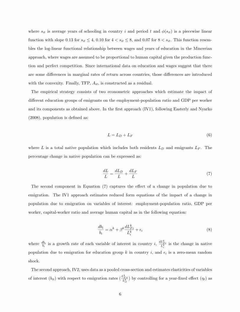
where sit is average years of schooling in country i and period t and φ(sit) is a piecewise linear
function with slope 0.13 for sit ≤ 4, 0.10 for 4 < sit ≤ 8, and 0.07 for 8 < sit. This function resem-
bles the log-linear functional relationship between wages and years of education in the Mincerian
approach, where wages are assumed to be proportional to human capital given the production func-
tion and perfect competition. Since international data on education and wages suggest that there
are some differences in marginal rates of return across countries, those differences are introduced
with the convexity. Finally, TFP, Ait, is constructed as a residual.
The empirical strategy consists of two econometric approaches which estimate the impact of
different education groups of emigrants on the employment-population ratio and GDP per worker
and its components as obtained above. In the first approach (IV1), following Easterly and Nyarko
(2008), population is defined as:
L = LD + LF (6)
where L is a total native population which includes both residents LD and emigrants LF . The
percentage change in native population can be expressed as:
dL
L=dLDL
+dLFL
(7)
The second component in Equation (7) captures the effect of a change in population due to
emigration. The IV1 approach estimates reduced form equations of the impact of a change in
population due to emigration on variables of interest: employment-population ratio, GDP per
worker, capital-worker ratio and average human capital as in the following equation:
dbibi
= αk + βkdLkF iLki
+ εi (8)
where dbibi
is a growth rate of each variable of interest in country i,dLk
Fi
Lki
is the change in native
population due to emigration for education group k in country i, and εi is a zero-mean random
shock.
The second approach, IV2, uses data as a pooled cross-section and estimates elasticities of variables
of interest (bit) with respect to emigration rates (LkFit
Lkit
) by controlling for a year-fixed effect (ηt) as
6

in the following equation:
ln bit = αk + ηt + γk lnLkF itLkit
+ εi (9)
3 Estimation Approach
This study estimates the impact of emigration on GDP per worker and its factors, obtained by a
production function decomposition and the employment-population ratio in migrant-sending coun-
tries using cross-country data over the period of 1990-2000. It analyzes the impact of emigration
for three different education groups of the native population: for all levels of education, those
with secondary and tertiary education, and those with tertiary education. Distinguishing across
these groups is important in understanding to what extent education of emigrants matters for de-
velopment of their home countries. Low-skill emigration can simply lead to a decline in labor or
influence countries of origin through remittances, promotion of FDI and trade, etc. In addition
to these channels, high-skill emigration directly reduces the level of human capital in the migrant-
sending countries but might contribute to investments in education, given a higher likelihood to
emigrate for individuals with more education, as emphasized in the literature.
Estimating these effects in reduced form equations in an Ordinary Least Squares (OLS) might
generate bias in the coefficients due to reverse causality or endogeneity. For example, emigration
of highly educated people might decrease GDP per worker in the source countries, given a higher
marginal productivity of high-skill labor compared to low-skill labor. At the same time, a low level
of GDP per worker might induce migration of more people both high-skilled and low-skilled to
higher-income countries with better standards of living. In terms of endogeneity, there might be
other factors driving both emigration and GDP per worker such as civil wars, weak institutions, etc.,
which might reduce GDP growth and increase emigration to countries with better opportunities.
To address these econometric problems this paper applies two different IV approaches. The first
approach introduces a new instrument, while the second approach uses conventional instruments
from the emigration literature. Comparing estimation results of these two approaches allows us to
test their robustness.
The first approach, IV1, studies how changes in native population due to emigration affect the
7

growth of the employment-population ratio, GDP per worker, capital-worker ratio, and average
human capital. Using this regressor helps to separate the impact of emigration from changes in
the structure of the domestic population. Migration to 30 OECD countries increased by 45 percent
over the period of 1990-2000 with similar trends observed across all education groups: primary (27
percent), secondary (51 percent), and tertiary (68 percent). However, these substantial changes in
absolute number of migrants had an insignificant impact on emigration rates in migrant sending
countries due to a rise in their population and education levels (Table 1). There was a 24.3
percent increase in the total population of migrant-sending countries with 19.6, 25.1, and 52.5
percent growth, respectively, in the number of primary, secondary, and tertiary educated people.
In addition, this approach estimates growth equations consisting of only time-variant variables,
thus eliminating countries’ fixed effects, omission of which can cause endogeneity bias.
Table 1: Emigration Rates in 1990 and 2000 by Education Groups1
Variable Mean Confidence Interval
Total Emigration Rate, 1990 .062 (0.047,0.077)
Total Emigration Rate, 2000 .067 (0.051,0.082)
Emigration Rate of Secondary and Tertiary Educated, 1990 .099 (0.078,0.120)
Emigration Rate of Secondary and Tertiary Educated, 2000 .101 (0.08,0.122)
Emigration Rate of Tertiary Educated, 1990 .208 (0.173,0.243)
Emigration Rate of Tertiary Educated, 2000 .194 (0.163,0.227)
The mean computed in the table is non-weighted arithmetic mean.
As OLS estimates of the reduced form equation (8) might be prone to simultaneity or omitted
variable bias, the IV technique is used to correct for this. Migrants’ networks and pull factors
of migration provide variations in emigration exogenous to migrant-sending countries’ conditions
and, therefore, can serve as a basis for constructing an instrument. There are economic incentives
for labor mobility between OECD countries and the rest of the world given a huge gap in income
levels. In these circumstances, migrants’ networks stimulate migration flows, as having individu-
als from the same countries of origin provides access to jobs and other information, substantially
reducing migration costs. Figure 1 in the Appendix depicts these network externalities, indicating
that countries with high emigration rates or with large diasporas in 1990 tend to have high emi-
1Emigration rates are computed for 195 migrant-sending countries in each year.
8
gration rates in 2000 as well. Each point on these graphs shows a share of emigrants in the total
native population in each migrant-sending country in 1990 and 2000 for three education levels:
all, secondary and tertiary, and tertiary, thus highlighting the key role of networks in a choice to
emigrate. In addition, Figure 2 illustrates the network effects for total emigration from India and
Philippines where distribution of migrants across major destination countries remains relatively
stable over time. Literature mostly discusses networks as a decisive factor in migrants’ location
choices in the context of subnational data and this study expands the existing literature by using
network effects for country level analysis. The growth in the total number of immigrants in each
of 30 destination countries, which might be a combination of different factors such as increases in
overall labor demand and changes in immigration policies, is also used to construct the instrument.
Assuming there are economic incentives for emigration from developing to developed countries, a
higher demand from destination countries triggers more emigration. At the same time, as migrants’
networks or diasporas play an important role in migrants’ destination choices, an increase in the
number of immigrants in the destination country from different countries of origin is likely to be
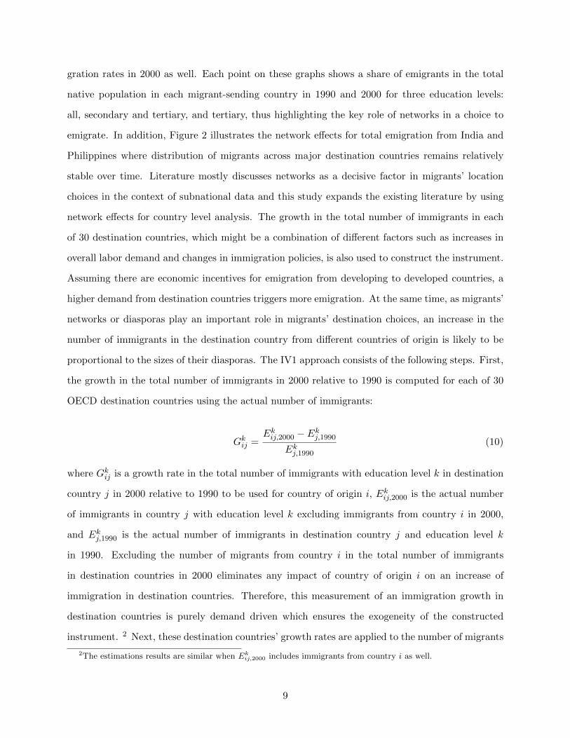
proportional to the sizes of their diasporas. The IV1 approach consists of the following steps. First,
the growth in the total number of immigrants in 2000 relative to 1990 is computed for each of 30
OECD destination countries using the actual number of immigrants:
Gkij =Ekij,2000 − Ekj,1990
Ekj,1990(10)
where Gkij is a growth rate in the total number of immigrants with education level k in destination
country j in 2000 relative to 1990 to be used for country of origin i, Ekij,2000 is the actual number
of immigrants in country j with education level k excluding immigrants from country i in 2000,
and Ekj,1990 is the actual number of immigrants in destination country j and education level k
in 1990. Excluding the number of migrants from country i in the total number of immigrants
in destination countries in 2000 eliminates any impact of country of origin i on an increase of
immigration in destination countries. Therefore, this measurement of an immigration growth in
destination countries is purely demand driven which ensures the exogeneity of the constructed
instrument. 2 Next, these destination countries’ growth rates are applied to the number of migrants
2The estimations results are similar when Ekij,2000 includes immigrants from country i as well.
9

from each country of origin i in the respective destination country j in 1990 in order to impute the
number of migrants in 2000:
Eki,j,2000 = Eki,j,1990 ×[1 +Gkij
](11)
where Eki,j,2000 is the imputed number of migrants from country of origin i in destination country j
with education level k in 2000, and Eki,j,1990 is the actual number of migrants from country of origin
i in destination country j with education level k in 1990. The imputed total number of emigrants
in each country of origin i is obtained by summing across the destination countries:
LkF,i,2000 =∑j
Eki,j,2000 (12)
Finally, the instrument for change in population due to emigration for each country i during the
period of 1990-2000 is constructed as:
dLk
F,i
Lki=LkF,i,2000 − LkF,i,1990
Lki,1990(13)
where LkF,i,1990 and Lki,1990 are respectively the actual number of emigrants and population in coun-
try i in 1990 with education level k. This instrument has a strong explanatory power for all
education levels of emigrants, as shown in Table 2.
Table 2: IV1, First-Stage Regression Results for Changes in Population due to Emigration byDifferent Education Groups
Dependent Variable Coefficient t-stat R-squared Observations
All Emigrants .940 16.06 0.572 195
Secondary and Tertiary Educated Emigrants .988 17.59 0.616 195
Tertiary Educated Emigrants 1.0 13.23 0.475 195
The second approach, IV2, uses data as a pooled cross-section for the years 1990 and 2000 and
studies the impact of emigration rates on the variables of interest for different education groups
as shown in equation (9). To address possible reverse causality and endogeneity issues, it applies
instruments selected from the emigration literature. The instruments for total emigration rates
10

include dummy variables for ever having been in a colonial relationship (Colony) and low-income
countries (Low Income); the average distance from destination countries, with the exception of
selective countries: Australia, Canada, and the U.S. (Distance); a minimum distance from selective
countries (Minimum Distance); and a country size, in terms of population including both residents
and emigrants (Population). Migrants are likely to face lower adjustment costs in the destination
country if the home country was its former colony due to similarity in institutions, language, and
stronger political ties. A dummy for low income countries is used as an instrument to capture
financial constraints of potential migrants which reduce their costly cross-country mobility. Also,
the physical distance between migrant-sending and receiving countries affects the travel costs for
the initial move and visits home. In addition, migrants are also better informed about neighboring
countries than distant ones. Distinguishing between selective and other countries is important in
the analysis of emigration by education groups, as around 63 percent of migrants with secondary
and tertiary education and 72 percent of migrants with tertiary education to 30 OECD countries
were hosted by selected countries in 2000. All destination countries with the exception of Australia,
Canada, the U.S., New Zealand and Mexico, are on the same continent and the average distance
is more indicative of migration costs. However, the minimum distance is more informative for
Australia, Canada and the U.S. given their highly dispersed locations. Finally, small countries
tend to be more open to emigration due to universal or nearly equal immigration quotas based
on countries of origin in migrant-receiving countries. The instruments for emigration rates of
secondary and tertiary educated groups vary. They include a dummy variable if the migrant-sending
country’s primary language is English (English), as it increases the transferability of migrants’ skills
for these education levels in the selective countries attracting most of them where English is an
official language. The dummy for low-income countries is dropped for these education groups since
emigrants with secondary and tertiary education are less financially constrained compared to the
emigrants with no formal education or only a primary education.
Tables 3 and 4 show the first-stage regression results for emigration rates by different education
groups with instruments discussed above for all countries and non-high-income countries. All in-
struments have the expected sign and significance. Emigration increases for all education groups
3In this and following tables the numbers in parentheses are standard errors of the coefficients and (*) indicatessignificance level at 10 percent, (**) at 5 percent, and (***) at 1 percent.
11

Table 3: IV2, First-Stage Regression Results for Emigration Rates by Education Groups: AllCountries
Instruments All Secondary and Tertiary Tertiary
Colony 0.582** (0.203) 3 0.723*** (0.21) 0.633** (0.203)
Low Income -0.932*** (0.195) -0.107 (0.176) 0.112 (0.169)
Distance -1.168*** (0.143) -0.680*** (0.117) -0.419*** (0.107)
Minimum Distance -1.252*** (0.237) -0.952*** (0.227) -0.583** (0.197)
Population -0.260*** (0.041) -0.254*** (0.037) -0.214*** (0.033)
English 0.431*** (0.125) 0.674*** (0.115)
Common Language 0.432** (0.15)
Observations 341 341 341
R-squared 0.458 0.383 0.354
Table 4: IV2, First-Stage Regression Results for Emigration Rates by Education Groups: Non-HighIncome Countries
Instruments All Secondary and Tertiary Tertiary
Colony 0.827*** (0.246) 0.913*** (0.241) 0.738** (0.232)
Low Income -0.666*** (0.189) 0.136 (0.162) 0.326* (0.158)
Distance -1.140*** (0.241) -0.796*** (0.176) -0.531*** (0.157)
Minimum Distance -2.007*** (0.2) -1.730*** (0.165) -1.216*** (0.142)
Population -0.195*** (0.046) -0.151*** (0.037) -0.120*** (0.034)
English 0.540*** (0.124) 0.828*** (0.114)
Common Language 0.076 (0.216)
Observations 247 247 247
R-squared 0.522 0.526 0.471
if a country has ever been in a colonial relationship (Colony). A dummy variable for low income
countries (Low Income) is significant and negative only for all emigrants, while it has no or low
explanatory power for higher education groups. The average distance to destination countries with
an exception of selected countries (Distance) and the minimum distance to selected emigration
countries (Minimum Distance) negatively affect emigration rates of all education groups. The re-
sults indicate that Mimium Distance is more important than Average Distance, given a high share
of migrants moving to selected destination countries and these estimates have overall lower mag-
nitudes for higher education levels. As expected, small countries are more open and emigration
rates decline with population (Population). To capture linguistic proximity and, therefore, lower
12
assimilation barriers, two variables are used: (i) a dummy variable if official or national languages
and languages spoken by at least 20 percent of the population of the country are spoken in the
destination country (Common Language) and (ii) a dummy variable if English is the official or
national language and language spoken at least by 20 percent of the population of the country (En-
glish). Using a dummy variable English instead of Common Language for more educated emigrants
is more relevant, as the majority of these emigrants are in three English-language destination coun-
tries: Australia, Canada and the U.S. and language is essential for skill transferability at higher
education levels. The results indicate that having a common language (Common Language) loses
significance when high-income countries are excluded from the sample, while the impact of variable
English remains positive and significant for both groups of countries and for both high education
levels. Based on these estimates, a dummy for low income countries (Low Income) is dropped from
the analysis of secondary and tertiary educated emigrants and tertiary educated emigrants, and
a dummy for commonly spoken language (Common Language) is removed from the list of instru-
ments for all emigrants. The remaining instruments have high explanatory power as can be seen
from the reported R2.
4 Data Description
This study uses the migration dataset by Docquier, Lowell, and Marfouk (2008) which provides
the number of migrants from 195 migrant-sending countries to 30 main destination OECD coun-
tries. These emigration stocks account for about 70 percent of total emigration and 90 percent
of skilled emigration in the world. The dataset classifies emigrants into three groups based on
education: high-skill, medium-skill, and low-skill emigrants with respectively a post-secondary, an
upper secondary, and a primary or no formal education. It also provides emigration rates for each
education group defined as a share of emigrants in the total native population including residents
and emigrants in the same education category.
Country-level aggregate variables including the employment-population ratio, GDP per worker,
capital per worker, and labor inputs are obtained from the Penn World Tables (PWT) by Heston,
Summers and Bettina (PWT 7.0). First, the number of workers in each country i and year t is
computed as (rgdpchit ∗ popit/rgdpwokit), where rgdpchit is a PPP converted GDP per capita
13

(Chain Series) at 2005 constant prices, popit is a population, and rgdpwokit is a PPP Converted
GDP Chain per worker at 2005 constant prices. To construct the employment-population ratio the
number of workers is divided by the population. The capital-worker rat io k is computed using the
perpetual inventory method:
Kit = Iit + δKit−1 (14)
where Iit is investment and δ is a depreciation rate. Iit is computed as (rgdplit ∗ popit ∗ kiit),
where rgdplit is a PPP converted GDP per capita (Laspeyres) at 2005 constant prices, popit is
population, and kiit is an investment share of PPP converted GDP per capita at 2005 constant
prices in country i and year t. The depreciation rate δ equals 0.06, which is a conventional value
used in the literature. In addition, PWT 7.0 provides data on several control variables discussed
below such as government size (kgit) and openness of the economy (openkit) measured respectively
as the shares of government expenditures and trade, including exports and imports, in GDP.
The average human capital hit is constructed using average years of schooling in the population
over 25 years old from the Barro - Lee dataset. As in Docquier and Marfouk (2006), human
capital indicators are replaced with those from De La Fuente and Domenech (2002) for OECD
countries. For countries where Barro and Lee measures are missing, the proportion of educated
individuals is predicted using the Cohen and Soto (2007) measures. In the result, there are 25
missing observations for 1990 and 35 for 2000 accounting respectively for 15 and 20 percent of
total observations, which are imputed using the GDP per worker. Finally, TFP is constructed as
a residual.
To obtain instruments for the IV2 approach, this study uses the GeoDist database by Mayer and
Zignago (2011), which provides information on colonial relationships, distance between countries
and countries’ spoken languages. Colonial relationship is defined as ever having been in a colonial
relationship. The distances are calculated following the great circle formula, which uses latitudes
and longitudes of the most important cities or agglomerations in terms of population. Finally,
spoken language is an official or national languages and languages spoken by at least 20 percent of
the population.
The control variables on legal origins of countries and political stability as described below are
14

taken from the Levine, Loayza and Beck (2000) dataset. The measurement of legal origins are
dummy variables for British, French, German and Scandinavian legal origins. The variables on
political stability include revolution and coups; assassinations; and ethnic fractionalization. A
revolution is defined as any illegal or forced change in the top governmental elite, any attempt
at such a change, or any successful or unsuccessful armed rebellion whose aim is independence
from the central government. Coup d’Etat is an extraconstitutional or forced change in the top
government elite and/or its effective control of the nation’s power structure in a given year. This
excludes unsuccessful coups, with data averaged over 1960-1990. The measurement of assassinations
is given by the average number of assassinations per thousand inhabitants over 1960-1990. Ethnic
fractionalization represents an average value of five indices of ethnolinguistic fractionalization with
values ranging from 0 to 1, where higher values denote higher levels of fractionalization.
5 Estimation Results
This paper studies emigrants’ impact on the GDP per worker and its production factors: capital-
worker ratio, average human capital, and TFP, and employment-population ratio. It estimates
equations (8) and (9) using the IV1 and IV2 econometric approaches described above for six country
groups based on the World Bank (WB) classification: (1) low income, (2) lower middle income,
(3) upper middle income, (4) all, (5) all non-high income, and (6) all low income and lower middle
income countries. To test the robustness of results, IV1 uses control variables adopted from Levine
et al. (2000) such as logarithms of the initial levels of the dependent variable and average human
capital in 1990. Next, it augments this list of regressors with growths in government size, measured
as a share of government expenditures in GDP and openness of the economy, computed as a trade
share in GDP. The IV2 approach first controls for logarithms of shares of government expenditures
and trade in GDP and then adds variables on financial development and political stability. Dummy
variables for British, French, German and Scandinavian legal origins exogenously drive differences
in the legal rules covering secured creditors, the efficiency of contract enforcement, and the quality
of accounting standards: hence, financial development. The number of revolutions and coups and
the number of assassinations per thousand of inhabitants averaged over 1960-1990 and an index of
ethnic fractionalization capture the variations in political stability.
15

Table 5 in the Appendix reports regression results of emigration impact on GDP per worker for
different education groups as in equations (8) and (9). In IV1 estimates, a one percent change
in native population due to total emigration increases GDP per worker for all countries by 2.1
percent at the 10 percent significance level; for all non-high income countries by 1.67 percent; and
for all low income and lower middle income countries by 1.88 percent at the 5 percent significance
level. These coefficients retain their significance and signs when adding control variables to the
regressions. Moreover, the signs and significance of these coefficients is consistent with the IV2
estimates, although their magnitudes differ. In particular, the GDP per worker grows in response
to an increase in total emigration rates for all countries by 0.69 percent; for all n’on-high income
countries by 0.46 percent; and for all low income and lower middle income countries by 0.45 percent.
The sensitivity analysis shows that this impact remains robust when control variables are included
in the regressions.
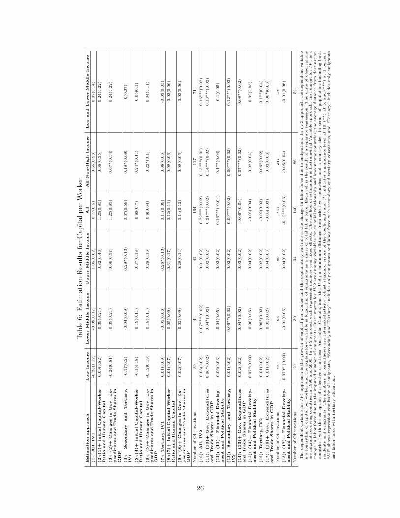
Decomposing the GDP per worker into capital per worker, human capital, and TFP helps to
understand the main channels of GDP growth driven by emigration. There is no robust significant
estimate of the impact of emigration on capital per worker across the IV1 and IV2 approaches
(Table 6). In the IV1 regressions, a change in population due to emigration of secondary and
tertiary educated individuals consistently raises capital per worker in all non-high income countries
with a magnitude in the range of 0.18-0.24 at the 10 percent significance level across different
specifications. In contrast, the results for IV2 indicate that there is an increase in capital per
worker in response to a one percent change in total emigration rates for all countries and all non-
high income countries across all estimates with a coefficient in the range of 0.1-0.22. There is no
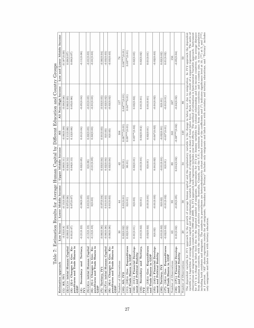
consistent significant estimate of emigration’s impact on human capital across different econometric
specifications in the IV1 approach (Table 7). In IV2, the only robust result is a positive impact of
total emigration rates on all countries with a coefficient in the range of 0.05-0.09. Table 8 reports
results for an impact of emigration rates for different education groups on the last component,
TFP. Similar to GDP per worker, TFP increases in all countries, all non-high income countries,
and all low and lower middle income countries in both IV1 and IV2 estimates. Thus, despite the
differences in IV1 and IV 2 estimation techniques and the inclusion of various control variables, some
results remain robust across all specifications. They indicate that migrant-sending countries’ GDP
per worker benefits from total emigration, mainly through improvements in TFP. These changes in
16

TFP might be a result of trade, FDI, and other cross-country partnerships facilitated by established
diasporas abroad which lead to a transfer of knowledge and technology.
This paper also studies the labor market implications of emigration for different education groups
by using both the IV1 and IV2 approaches to estimate the impact of emigration on the employment-
population ratio. Overall, there is no consistent significant estimate of this impact across differ-
ent education groups and specifications. The IV1 estimation results in Table 9 indicate that the
employment-population ratio declines by 0.17-0.21 percent in response to a one percent change in
population of secondary and tertiary educated due to emigration for upper middle income countries.
However, there is no significant change in the employment-population ratio of other income groups
across different education levels. The IV2 estimates produce no consistent significant results across
different specifications. In addition, the results for GDP per worker can serve as a basis for wage
analysis. In the conditions of perfect competition and constant returns to scale, wages are equal
to the marginal product of labor, expressed as (1 − α) YitLit. Therefore, wages rise in response to an
increase in total emigration rates in all countries, all non-high income countries, and all low and
lower middle income countries.
6 Conclusions
This paper studies the impact of emigration on several macroeconomic variables of migrant-sending
countries using 1990 and 2000 emigration data from 195 source countries to 30 OECD destination
countries. It applies two econometric approaches varying by the choice of instruments and specifica-
tions. The first approach studies the impact of changes in the native population due to emigration
on the growth of employment-population ratio, GDP per worker, and its components. To overcome
the endogeneity bias, it uses instruments based on migration pull factors and migrants’ networks.
The second approach estimates the elasticities of variables of interest with respect to emigration
rates, using conventional instruments from the literature such as colonial relationship, distance,
country size, country’s development level, and English as a primary language. Estimation results
indicate that total emigration rates increase GDP per worker in all countries, non-high income
countries, and low and lower middle income countries: an effect primarily driven by improvements
in TFP. These results are robust to both econometric approaches and inclusion of various con-
17

trol variables in the regressions. In addition, emigration has no consistent significant impact on
migrant-sending countries’ employment-population ratio across different specifications.
18

References
[1] Acosta, P., C. Calderon, P. Fajnzylber and H. Lopez (2008): What is the Impact of Interna-
tional Remittances on Poverty and Inequality in Latin America?, World Development, 36, 1:
89-114.
[2] Adams, R. H. Jr. (1998): Investment, and Rural Asset Accumulation in Pakistan, Economic
Development and Cultural Change, 47, 1: 155-173.
[3] Aydemir, A., and G. J. Borjas (2007): A comparative analysis of the labor market impact
of international migration: Canada, Mexico, and the United States, Journal of the European
Economic Association, 5, 4: 663-08.
[4] Barajas, A., R. Chami, C. Fullenkamp, M. Gapen and P. Montiel (2009): Do Workers’ Remit-
tances Promote Economic Growth?, IMF Working Paper, WP/09/153.
[5] Beine, M., F. Docquier and C. Oden-Defoort (2011): A Panel Data Analysis of The Brain
Gain, World Development, forthcoming.
[6] Beine, M., F. Docquier and C. Ozden (2011): Diasporas, Journal of Development Economics,
95, 1: 30-41.
[7] Beine, M., F. Docquier and H. Rapoport (2001): Brain drain and economic growth: theory
and evidence, Journal of Development Economics, 64, 1: 275-89.
[8] Beine, M., F. Docquier and H. Rapoport (2007): Measuring international skilled migration:
new estimates controlling for age of entry, World Bank Economic Review, 21, 2: 249-54.
[9] Beine, M., F. Docquier and H. Rapoport (2008): Brain drain and human capital formation in
developing countries: winners and losers, Economic Journal, 118: 631-652.
[10] Card, D. (2001): Immigrant Inflows, Native Outflows, and the Local Market Impacts of Higher
Immigration, Journal of Labor Economics 19: 22-64.
[11] Catrinescu, N., M. Leon-Ledesma, M. Piracha and B. Quillin (2009): Remittances, Institu-
tions, and Economic Growth, World Development 37, 1: 81-92.
19

[12] Caselli, F. (2005): Accounting for Cross-Country Income Differences, Handbook of Economic
Growth, in: Philippe Aghion and Steven Durlauf (ed.), Handbook of Economic Growth, edition
1, volume 1, chapter 9: 679-741. Elsevier.
[13] Chami, R., D. Hakura and P. Montiel (2009): Remittances: An Automatic Output Stabilizer?,
IMF Working Paper, WP/09/91.
[14] Cox, A. and M. Ureta (2003): International migration, remittances and schooling: evidence
from El Salvador, Journal of Development Economics, 72, 2: 429-461.
[15] Docquier, F., O. Faye and P. Pestieau (2008): Is migration a good substitute for subsidies,
Journal of Development Economics, 86, 2: 263-76.
[16] Docquier, F., O. Lohest and A. Marfouk (2007): Brain drain in developing countries, World
Bank Economic Review, 21, 2: 193-218.
[17] Docquier, F., B. L. Lowell and A. Marfouk (2009): A gendered assessment of the brain drain,
Population and Development Review, 35, 2: 297-321.
[18] Docquier, F. and A. Marfouk (2006): International migration by educational attainment (1990-
2000), in C. Ozden and M. Schiff (eds): International Migration, Remittances and Develop-
ment, Palgrave Macmillan: New York.
[19] Easterly, W. and Y. Nyarko (2009): Is the Brain Drain Good for Africa? Chapter 11 in J.
Bhagwati and G. Hanson (eds): Skilled immigration: problems, prospects and policies, Oxford
University Press: 316-60.
[20] Gould, D. M. (1994): Immigration links to the home country: Empirical implications for U.S.
bilateral trade flows, Review of Economics and Statistics, 76: 302-316.
[21] Grogger, J. and G. Hanson (2011): Income maximization and the selection and sorting of
international migrants, Journal of Development Economics, 95, 1: 42-57.
[22] Grubel, H. and A. Scott (1966): The international flow of human capital, American Economic
Review, 56: 268-74.
[23] Hanson, G. H. (2007): International Migration and the Developing World, Mimeo, UCSD.
20
[24] Head, K., J. Ries and D. Swenson (1998): Immigration and trade creation: Econometric
evidence from Canada, Canadian Journal of Economics, 31, 1: 47-62.
[25] Hildebrandt, N. and D. McKenzie (2005): The effects of migration on child health in Mexico,
World Bank Policy Research Working Paper, 3573.
[26] Levine, R., N. Loayza and T. Beck (2000): Financial intermediation and growth: Causality
and causes, Journal of Monetary Economics, 46: 31-77.
[27] Mayda, A.M. (2010): International migration: a panel data analysis of the determinants of
bilateral flows, Journal of Population Economics, 23, 4: 1249-74.
[28] Mishra, P. (2007): Emigration and wages in source countries: Evidence from Mexico, Journal
of Development Economics, 82, 1: 180-199.
[29] Nielsen, M. E., andP. Olinto (2007): Do Conditional Cash Transfers Crowd Out Private Trans-
fers? in P. Fajnzylber and H. Lopez (eds.): Remittances and Development: Lessons from Latin
America, The World Bank, Washington, DC: 253-298.
[30] Saxenian, A. (1999): Silicon Valley’s new immigrant entrepreneurs, Public Policy Institute of
California.
[31] Teruel, G. and B. Davis (2000): Final report: An evaluation of the impact of PROGRESA cash
payments on private inter-household transfers, International Food Policy Research Institute.
[32] Woodruff, C., and R. Zenteno (2007): Migration networks and microenterprises in Mexico,
Journal of Development Economics, 82, 2: 509-528.
[33] Yang, D. (2008): International migration, remittances, and household investment: Evidence
from Philippine migrants’ exchange rate shocks, Economic Journal, 118, 528: 591-630.
notes://NOTES303/85257726004C7554/38D46BF5E8F08834852564B500129B2C/2D7D81B0DD8ACA4F85257B9C007BD901
7 Appendix
21

Figure 1: Share of Emigrants in Native Population across Countries by Different Education Groupsin 1990 and 2000.
0%
10%
20%
30%
40%
50%
60%
0% 10% 20% 30% 40% 50%
2000
1990
All Emigrants
0%
10%
20%
30%
40%
50%
60%
70%
80%
90%
0% 10% 20% 30% 40% 50% 60% 70% 80%
2000
1990
Emigrants with Secondary and Tertiary Education
22

0%
10%
20%
30%
40%
50%
60%
70%
80%
90%
100%
0% 10% 20% 30% 40% 50% 60% 70% 80% 90% 100%
2000
1990
Emigrants with Tertiary Education
23

Figure 2: Total Number of Emmigrants in India and Philippines in 1990 and 2000 by MajorDestination Countries.
0
200,000
400,000
600,000
800,000
1,000,000
1,200,000
1,400,000
1,600,000
Philippines, 1990 Philippines, 2000 India, 1990 India, 2000
UK
Germany
USA
Canada
Australia
Italy
Japan
Peo
ple
24

Tab
le5:
Est
imat
ion
Res
ult
sfo
rG
DP
per
Wor
ker
Estim
atio
napproach
Low
Incom
eLower
Mid
dle
Incom
eU
pper
Mid
dle
Incom
eA
llA
llN
on-H
igh
Incom
eLow
and
Lower
Mid
dle
Incom
e
(1):
All,IV
10.0
7(2
.45)
1.6
51*(0
.66)
0.8
4(0
.89)
2.1
*(0
.81)
1.6
7**(0
.55)
1.8
8**
(0.6
)
(2):(1)+
initia
lG
DP
per
Worker
and
Hum
an
Capital
2.5
(2.2
4)
2.3
3***(0
.62)
0.9
1(0
.96)
2.1
5*(0
.96)
1.6
6**(0
.6)
2.1
5**(0
.67)
(3):
(2)+
Changes
inG
ov.
Ex-
pendituresand
Trade
Sharesin
GD
P
1.2
9(1
.62)
2.3
5***(0
.64)
0.3
7(0
.9)
2.1
7*(1
)1.5
8**(0
.59)
2.1
7**(0
.7)
(4):
Secondary
and
Tertia
ry,
IV
1-0
.57(0
.43)
0.9
*(0
.44)
0.0
1(0
.3)
1.2
2(0
.87)
0.4
9(0
.26)
0.8
(0.4
)
(5):(4)+
initia
lG
DP
per
Worker
and
Hum
an
Capital
-0.1
9(0
.53)
1.1
5*(0
.43)
0.2
(0.3
4)
1.2
7(0
.89)
0.4
7(0
.25)
0.8
1(0
.43)
(6):
(5)+
Changes
inG
ov.
Ex-
pendituresand
Trade
Sharesin
GD
P
-0.2
9(0
.47)
1.1
6*(0
.45)
0.0
1(0
.32)
1.1
9(0
.84)
0.4
2(0
.25)
0.8
(0.4
5)
(7):
Tertia
ry,IV
1-0
.07(0
.19)
0.5
8*(0
.28)
0.1
4(0
.22)
0.2
7(0
.18)
0.2
2(0
.16)
0.2
5(0
.23)
(8):(7)+
initia
lG
DP
per
Worker
and
Hum
an
Capital
0.0
4(0
.21)
0.6
6*(0
.31)
0.3
4(0
.3)
0.2
5(0
.15)
0.1
9(0
.15)
0.2
1(0
.22)
(9):
(8)+
Changes
inG
ov.
Ex-
pendituresand
Trade
Sharesin
GD
P
0.0
9(0
.22)
0.6
6*(0
.32)
0.2
(0.2
9)
0.2
9(0
.18)
0.1
8(0
.15)
0.2
3(0
.23)
Num
ber
of
Obse
rvati
ons
30
44
42
164
117
74
(10):
All,IV
20.1
6(0
.08)
0.1
7***(0
.04)
0.0
9(0
.05)
0.6
9***(0
.07)
0.4
6***(0
.05)
0.4
5***(0
.06)
(11):(10)+
Gov.Expenditures
and
Trade
Shares
inG
DP
0.1
8(0
.09)
0.1
5**(0
.04)
0.1
1(0
.07)
0.6
7***(0
.08)
0.4
4***(0
.05)
0.3
9***(0
.06)
(12):
(11)+
Fin
ancia
lD
evelo
p-
ment
and
Politic
alStabiity
0.2
1(0
.11)
0.2
5(0
.2)
0.0
3(0
.06)
0.5
1***(0
.13)
0.3
7*(0
.14)
0.4
4*(0
.19)
(13):
Secondary
and
Tertia
ry,
IV
20.0
2(0
.1)
0.1
6***(0
.05)
0.1
(0.0
6)
0.2
5**(0
.08)
0.2
7***(0
.05)
0.3
1***(0
.08)
(14):(13)+
Gov.Expenditures
and
Trade
Shares
inG
DP
0.0
3(0
.1)
0.1
3**(0
.04)
0.1
4(0
.07)
0.2
*(0
.09)
0.2
2***(0
.06)
0.2
2**
(0.0
8)
(15):
(14)+
Fin
ancia
lD
evelo
p-
ment
and
Politic
alStabiity
0.3
3**(0
.1)
0.2
8(0
.17)
0.0
5(0
.06)
-0.0
6(0
.14)
0.1
2(0
.14)
0.1
7(0
.18)
(16):
Tertia
ry,IV
2-0
.03(0
.09)
0.1
5*(0
.06)
0.1
(0.0
7)
-0.1
2(0
.09)
0.1
4(0
.07)
0.2
27*(0
.1)
(17):(16)+
Gov.Expenditures
and
Trade
Shares
inG
DP
-0.0
3(0
.09)
0.1
1*(0
.05)
0.1
5(0
.09)
-0.2
2*(0
.1)
0.0
7(0
.07)
0.1
5(0
.09)
Num
ber
of
Obse
rvati
ons
63
93
89
341
247
156
(18):
(17)+
Fin
ancia
lD
evelo
p-
ment
and
Politic
alStabiity
0.3
7**(0
.1)
0.1
4(0
.23)
0.0
5(0
.06)
-0.3
8**(0
.13)
-0.0
8(0
.16)
0.0
8(0
.22)
Num
ber
of
Obse
rvati
ons
20
30
34
140
86
50
The
dep
endent
vari
able
forIV
1appro
ach
isth
egro
wth
of
GD
Pp
er
work
er
and
the
expla
nato
ryvari
able
isth
echange
inla
bor
forc
edue
toem
igra
tion.
InIV
2appro
ach
the
dep
endent
vari
able
isa
logari
thm
of
GD
Pp
er
work
er
and
the
expla
nato
ryvari
able
islo
gari
thm
of
em
igra
nts
as
ash
are
of
tota
lla
bor
forc
e.
Each
cell
isth
ere
sult
of
ase
para
tere
gre
ssio
n.
The
unit
sof
obse
rvati
ons
are
mig
rant
receiv
ing
countr
ies
in1990
and
2000.
InIV
2appro
ach
each
regre
ssio
nin
clu
des
year
fixed
eff
ects
.T
he
meth
od
of
est
imati
on
isIn
stru
menta
lV
ari
able
appro
ach.
Inst
rum
ent
forIV
1is
achange
inla
bor
forc
edue
toth
eim
pute
dnum
ber
of
em
igra
nts
.In
stru
ments
forIV
2are
dum
my
vari
able
sfo
rcolo
nia
lre
lati
onsh
ipand
low
-incom
ecountr
ies;
the
avera
ge
dis
tance
from
dest
inati
on
countr
ies,
wit
hth
eexcepti
on
of
sele
cti
ve
countr
ies:
Aust
ralia,
Canada,
and
the
U.S
.;a
min
imum
dis
tance
from
sele
cti
ve
countr
ies;
and
acountr
ysi
ze,
inte
rms
of
popula
tion
inclu
din
gb
oth
resi
dents
and
em
igra
nts
.T
he
num
bers
inpare
nth
ese
sare
hete
rosk
edast
icit
yro
bust
standard
err
ors
of
the
coeffi
cie
nts
and
(*)
indic
ate
ssi
gnifi
cance
level
at
10,
(**)
at
5,
and
(***)
at
1p
erc
ent.
“A
ll”
show
sre
gre
ssio
nre
sult
sfo
rall
em
igra
nts
,“Secondary
and
Tert
iary
”in
clu
des
only
em
igra
nts
and
lab
or
forc
ew
ith
secondary
and
tert
iary
educati
ons,
and
“T
ert
iary
”in
clu
des
only
em
igra
nts
and
lab
or
forc
ew
ith
tert
iary
educati
on.
25
Tab
le6:
Est
imat
ion
Res
ult
sfo
rC
apit
alp
erW
orker
Estim
atio
napproach
Low
Incom
eLower
Mid
dle
Incom
eU
pper
Mid
dle
Incom
eA
llA
llN
on-H
igh
Incom
eLow
and
Lower
Mid
dle
Incom
e
(1):
All,IV
1-0
.23(1
.12)
-0.0
9(0
.17)
1.0
5(0
.62)
0.7
7(0
.5)
0.5
5(0
.28)
0.0
7(0
.14)
(2):(1)+
initia
lCapital-W
orker
Ratio
and
Hum
an
Capital
0.0
9(0
.82)
0.3
9(0
.21)
0.8
2(0
.46)
1.2
3(0
.85)
0.6
8(0
.35)
0.2
4(0
.22)
(3):
(2)+
Changes
inG
ov.
Ex-
pendituresand
Trade
Sharesin
GD
P
-0.2
4(0
.81)
0.3
9(0
.21)
0.6
6(0
.37)
1.2
2(0
.83)
0.6
7*(0
.34)
0.2
4(0
.22)
(4):
Secondary
and
Tertia
ry,
IV
1-0
.17(0
.2)
-0.0
4(0
.09)
0.2
9*(0
.13)
0.6
7(0
.59)
0.1
8*(0
.09)
0(0
.07)
(5):(4)+
initia
lCapital-W
orker
Ratio
and
Hum
an
Capital
-0.1
(0.1
8)
0.1
9(0
.11)
0.3
7(0
.18)
0.8
6(0
.7)
0.2
4*(0
.11)
0.0
5(0
.1)
(6):
(5)+
Changes
inG
ov.
Ex-
pendituresand
Trade
Sharesin
GD
P
-0.1
2(0
.19)
0.1
8(0
.11)
0.2
8(0
.16)
0.8
(0.6
4)
0.2
2*(0
.1)
0.0
4(0
.11)
(7):
Tertia
ry,IV
10.0
1(0
.09)
-0.0
5(0
.06)
0.2
6*(0
.13)
0.1
1(0
.09)
0.0
8(0
.06)
-0.0
3(0
.05)
(8):(7)+
initia
lCapital-W
orker
Ratio
and
Hum
an
Capital
0.0
1(0
.07)
0.0
5(0
.09)
0.3
1(0
.17)
0.1
2(0
.11)
0.0
8(0
.06)
-0.0
3(0
.06)
(9):
(8)+
Changes
inG
ov.
Ex-
pendituresand
Trade
Sharesin
GD
P
0.0
2(0
.07)
0.0
2(0
.09)
0.2
8(0
.14)
0.1
4(0
.12)
0.0
8(0
.06)
-0.0
3(0
.06)
Num
ber
of
Obse
rvati
ons
30
44
42
164
117
74
(10):
All,IV
20.0
5(0
.02)
0.0
7***(0
.02)
0.0
1(0
.02)
0.2
2***(0
.02)
0.1
5***(0
.01)
0.1
6***(0
.02)
(11):(10)+
Gov.Expenditures
and
Trade
Shares
inG
DP
0.0
6*(0
.02)
0.0
4*(0
.02)
0.0
2(0
.02)
0.2
1***(0
.02)
0.1
4***(0
.02)
0.1
3***(0
.02)
(12):
(11)+
Fin
ancia
lD
evelo
p-
ment
and
Politic
alStabiity
0.0
6(0
.03)
0.0
4(0
.05)
0.0
2(0
.02)
0.1
6***(-
0.0
4)
0.1
**(0
.04)
0.1
(0.0
5)
(13):
Secondary
and
Tertia
ry,
IV
20.0
1(0
.02)
0.0
6**(0
.02)
0.0
2(0
.02)
0.0
9***(0
.02)
0.0
9***(0
.02)
0.1
2***(0
.03)
(14):(13)+
Gov.Expenditures
and
Trade
Shares
inG
DP
0.0
2(0
.02)
0.0
4*(0
.02)
0.0
3(0
.02)
0.0
6*(0
.03)
0.0
7***(0
.02)
0.0
8**(0
.02)
(15):
(14)+
Fin
ancia
lD
evelo
p-
ment
and
Politic
alStabiity
0.0
7*(0
.03)
0.0
6(0
.05)
0.0
4(0
.02)
-0.0
3(0
.04)
0.0
2(0
.04)
0.0
2(0
.05)
(16):
Tertia
ry,IV
20.0
1(0
.02)
0.0
6*(0
.03)
0.0
2(0
.02)
-0.0
2(0
.03)
0.0
6*(0
.02)
0.1
**(0
.04)
(17):(16)+
Gov.Expenditures
and
Trade
Shares
inG
DP
0.0
1(0
.02)
0.0
3(0
.02)
0.0
4(0
.03)
-0.0
6(0
.03)
0.0
3(0
.03)
0.0
6*(0
.03)
Num
ber
of
Obse
rvati
ons
63
93
89
341
247
156
(18):
(17)+
Fin
ancia
lD
evelo
p-
ment
and
Politic
alStabiity
0.0
79*
(0.0
3)
-0.0
1(0
.05)
0.0
4(0
.02)
-0.1
2***(0
.03)
-0.0
5(0
.04)
-0.0
1(0
.06)
Num
ber
of
Obse
rvati
ons
20
30
34
140
86
50
The
dep
endent
vari
able
forIV
1appro
ach
isth
egro
wth
of
capit
al
per
work
er
and
the
expla
nato
ryvari
able
isth
echange
inla
bor
forc
edue
toem
igra
tion.
InIV
2appro
ach
the
dep
endent
vari
able
isa
logari
thm
of
capit
al
per
work
er
and
the
expla
nato
ryvari
able
islo
gari
thm
of
em
igra
nts
as
ash
are
of
tota
lla
bor
forc
e.
Each
cell
isth
ere
sult
of
ase
para
tere
gre
ssio
n.
The
unit
sof
obse
rvati
ons
are
mig
rant
receiv
ing
countr
ies
in1990
and
2000.
InIV
2appro
ach
each
regre
ssio
nin
clu
des
year
fixed
eff
ects
.T
he
meth
od
of
est
imati
on
isIn
stru
menta
lV
ari
able
appro
ach.
Inst
rum
ent
forIV
1is
achange
inla
bor
forc
edue
toth
eim
pute
dnum
ber
of
em
igra
nts
.In
stru
ments
forIV
2are
dum
my
vari
able
sfo
rcolo
nia
lre
lati
onsh
ipand
low
-incom
ecountr
ies;
the
avera
ge
dis
tance
from
dest
inati
on
countr
ies,
wit
hth
eexcepti
on
of
sele
cti
ve
countr
ies:
Aust
ralia,
Canada,
and
the
U.S
.;a
min
imum
dis
tance
from
sele
cti
ve
countr
ies;
and
acountr
ysi
ze,
inte
rms
of
popula
tion
inclu
din
gb
oth
resi
dents
and
em
igra
nts
.T
he
num
bers
inpare
nth
ese
sare
hete
rosk
edast
icit
yro
bust
standard
err
ors
of
the
coeffi
cie
nts
and
(*)
indic
ate
ssi
gnifi
cance
level
at
10,
(**)
at
5,
and
(***)
at
1p
erc
ent.
“A
ll”
show
sre
gre
ssio
nre
sult
sfo
rall
em
igra
nts
,“Secondary
and
Tert
iary
”in
clu
des
only
em
igra
nts
and
lab
or
forc
ew
ith
secondary
and
tert
iary
educati
ons,
and
“T
ert
iary
”in
clu
des
only
em
igra
nts
and
lab
or
forc
ew
ith
tert
iary
educati
on.
26
Tab
le7:
Est
imati
on
Res
ult
sfo
rA
ver
age
Hu
man
Cap
ital
by
Diff
eren
tE
du
cati
onan
dC
ountr
yG
rou
ps
Estim
atio
napproach
Low
Incom
eLower
Mid
dle
Incom
eU
pper
Mid
dle
Incom
eA
llA
llN
on-H
igh
Incom
eLow
and
Lower
Mid
dle
Incom
e
(1):
All,IV
1-0
.53(0
.8)
-0.1
5(0
.09)
0.0
9(0
.11)
-0.0
6(0
.09)
-0.0
9(0
.08)
-0.1
8*(0
.09)
(2):(1)+
initia
lH
um
an
Capital
-0.0
9(0
.48)
0.0
7(0
.06)
0.0
4(0
.14)
0.1
1(0
.06)
0.0
6(0
.05)
0.0
9(0
.07)
(3):
(2)+
Changes
inG
ov.
Ex-
pendituresand
Trade
Sharesin
GD
P
0.0
1(0
.47)
0.0
7(0
.07)
0.0
4(0
.13)
0.1
2(0
.06)
0.0
5(0
.06)
0.0
9(0
.07)
(4):
Secondary
and
Tertia
ry,
IV
1-0
.21(0
.22)
-0.0
8(0
.05)
0.0
2(0
.05)
0.0
1(0
.04)
-0.0
5(0
.04)
-0.1
1(0
.06)
(5):(4)+
initia
lH
um
an
Capital
-0.1
5(0
.18)
0.0
1(0
.03)
0(0
.06)
0.0
2(0
.03)
-0.0
1(0
.03)
-0.0
1(0
.03)
(6):
(5)+
Changes
inG
ov.
Ex-
pendituresand
Trade
Sharesin
GD
P
-0.1
5(0
.18)
0(0
.03)
-0.0
1(0
.05)
0.0
2(0
.03)
-0.0
1(0
.03)
-0.0
1(0
.03)
(7):
Tertia
ry,IV
1-0
.06(0
.06)
-0.0
7(0
.04)
0.0
3(0
.04)
0.0
1(0
.03)
-0.0
3(0
.03)
-0.0
6(0
.04)
(8):(7)+
initia
lH
um
an
Capital
-0.0
6(0
.06)
0.0
1(0
.03)
0.0
2(0
.04)
0(0
.03)
-0.0
2(0
.02)
-0.0
3(0
.03)
(9):
(8)+
Changes
inG
ov.
Ex-
pendituresand
Trade
Sharesin
GD
P
-0.0
6(0
.06)
0.0
1(0
.03)
0.0
2(0
.04)
0(0
.03)
-0.0
2(0
.02)
-0.0
3(0
.03)
Num
ber
of
Obse
rvati
ons
30
44
42
164
117
74
(10):
All,IV
20.0
2(0
.02)
0.0
1(0
.01)
0(0
.01)
0.0
8***(0
.01)
0.0
4***(0
.01)
0.0
4***(0
.01)
(11):(10)+
Gov.Expenditures
and
Trade
Shares
inG
DP
0.0
2(0
.02)
0(0
.01)
00.0
1)
0.0
9***(0
.01)
0.0
4***0.0
1)
0.0
3**(0
.01)
(12):
(11)+
Fin
ancia
lD
evelo
p-
ment
and
Politic
alStabiity
0.0
1(0
.01)
0(0
.03)
0.0
2(0
.01)
0.0
5**(0
.02)
0.0
3(0
.02)
0.0
2(0
.03)
(13):
Secondary
and
Tertia
ry,
IV
2-0
.01(0
.02)
0(0
.01)
-0.0
1(0
.01)
0.0
2(0
.012)
0.0
1(0
.01)
0.0
2(0
.02)
(14):(13)+
Gov.Expenditures
and
Trade
Shares
inG
DP
-0.0
2(0
.02)
-0.0
1(0
.01)
0(0
.01)
0.0
2(0
.01)
0.0
1(0
.01)
0.0
1(0
.01)
(15):
(14)+
Fin
ancia
lD
evelo
p-
ment
and
Politic
alStabiity
0(0
.02)
-0.0
1(0
.03)
0.0
1(0
.02)
-0.0
4*(0
.02)
-0.0
1(0
.02)
-0.0
2(0
.03)
(16):
Tertia
ry,IV
2-0
.01(0
.02)
0(0
.02)
-0.0
1(0
.01)
-0.0
2(0
.01)
0(0
.01)
0.0
2(0
.02)
(17):(16)+
Gov.Expenditures
and
Trade
Shares
inG
DP
-0.0
2(0
.02)
-0.0
1(0
.02)
0(0
.01)
-0.0
3*(0
.01)
-0.0
1(0
.01)
0.0
1(0
.02)
Num
ber
of
Obse
rvati
ons
63
93
89
341
247
156
(18):
(17)+
Fin
ancia
lD
evelo
p-
ment
and
Politic
alStabiity
0.0
1(0
.02)
-0.0
5(0
.05)
0.0
14(0
.02)
-0.0
8***(0
.02)
-0.0
4(0
.02)
-0.0
5(0
.04)
Num
ber
of
Obse
rvati
ons
20
30
34
140
86
50
The
dep
endent
vari
able
forIV
1appro
ach
isth
egro
wth
of
avera
ge
hum
an
capit
al
and
the
expla
nato
ryvari
able
isth
echange
inla
bor
forc
edue
toem
igra
tion.
InIV
2appro
ach
the
dep
endent
vari
able
isa
logari
thm
of
avera
ge
hum
an
capit
al
and
the
expla
nato
ryvari
able
islo
gari
thm
of
em
igra
nts
as
ash
are
of
tota
lla
bor
forc
e.
Each
cell
isth
ere
sult
of
ase
para
tere
gre
ssio
n.
The
unit
sof
obse
rvati
ons
are
mig
rant
receiv
ing
countr
ies
in1990
and
2000.
InIV
2appro
ach
each
regre
ssio
nin
clu
des
year
fixed
eff
ects
.T
he
meth
od
of
est
imati
on
isIn
stru
menta
lV
ari
able
appro
ach.
Inst
rum
ent
forIV
1is
achange
inla
bor
forc
edue
toth
eim
pute
dnum
ber
of
em
igra
nts
.In
stru
ments
forIV
2are
dum
my
vari
able
sfo
rcolo
nia
lre
lati
onsh
ipand
low
-incom
ecountr
ies;
the
avera
ge
dis
tance
from
dest
inati
on
countr
ies,
wit
hth
eexcepti
on
of
sele
cti
ve
countr
ies:
Aust
ralia,
Canada,
and
the
U.S
.;a
min
imum
dis
tance
from
sele
cti
ve
countr
ies;
and
acountr
ysi
ze,
inte
rms
of
popula
tion
inclu
din
gb
oth
resi
dents
and
em
igra
nts
.T
he
num
bers
inpare
nth
ese
sare
hete
rosk
edast
icit
yro
bust
standard
err
ors
of
the
coeffi
cie
nts
and
(*)
indic
ate
ssi
gnifi
cance
level
at
10,
(**)
at
5,
and
(***)
at
1p
erc
ent.
“A
ll”
show
sre
gre
ssio
nre
sult
sfo
rall
em
igra
nts
,“Secondary
and
Tert
iary
”in
clu
des
only
em
igra
nts
and
lab
or
forc
ew
ith
secondary
and
tert
iary
educati
ons,
and
“T
ert
iary
”in
clu
des
only
em
igra
nts
and
lab
or
forc
ew
ith
tert
iary
educati
on.
27

Tab
le8:
Est
imati
onR
esu
lts
for
TF
Pby
Diff
eren
tE
du
cati
onan
dC
ountr
yG
roup
sEstim
atio
napproach
Low
Incom
eLower
Mid
dle
Incom
eU
pper
Mid
dle
Incom
eA
llA
llN
on-H
igh
Incom
eLow
and
Lower
Mid
dle
Incom
e
(1):
All,IV
10.8
3(2
.17)
1.8
9**(0
.64)
-0.3
1(0
.57)
1.3
9**(0
.52)
1.2
1*(0
.49)
1.9
8**(0
.59)
(2):(1)+
initia
lTFP
and
Hu-
man
Capital
2.2
1(1
.84)
1.9
5**(0
.56)
-0.0
8(0
.49)
1.1
2*(0
.46)
1.0
7*(0
.47)
1.9
6**(0
.61)
(3):
(2)+
Changes
inG
ov.
Ex-
pendituresand
Trade
Sharesin
GD
P
1.4
(1.4
)1.9
6**(0
.57)
-0.4
9(0
.56)
1.0
6*(0
.47)
0.7
6*(0
.46)
1.9
7**(0
.62)
(4):
Secondary
and
Tertia
ry,
IV
1-0
.19(0
.4)
1.0
2*(0
.45)
-0.3
(0.2
6)
0.5
5(0
.34)
0.3
6(0
.26)
0.9
2*(0
.41)
(5):(4)+
initia
lTFP
and
Hu-
man
Capital
0.0
5(0
.44)
1*(0
.39)
-0.1
7(0
.19)
0.5
2(0
.32)
0.3
(0.2
3)
0.8
3*(0
.39)
(6):
(5)+
Changes
inG
ov.
Ex-
pendituresand
Trade
Sharesin
GD
P
0(0
.4)
1.0
2*(0
.38)
-0.2
8(0
.19)
0.4
6(0
.31)
0.2
6(0
.23)
0.8
2*(0
.4)
(7):
Tertia
ry,IV
1-0
.02(0
.16)
0.7
*(0
.27)
-0.1
4(0
.17)
0.1
5(0
.15)
0.1
6(0
.16)
0.3
4(0
.24)
(8):(7)+
initia
lTFP
and
Hu-
man
Capital
0.0
8(0
.18)
0.6
5*(0
.27)
-0.0
1(0
.14)
0.1
5(0
.12)
0.1
3(0
.14)
0.2
8(0
.21)
(9):
(8)+
Changes
inG
ov.
Ex-
pendituresand
Trade
Sharesin
GD
P
0.1
3(0
.21)
0.6
7*(0
.27)
-0.1
4(0
.15)
0.1
5(0
.13)
0.1
1(0
.13)
0.2
9(0
.21)
Num
ber
of
Obse
rvati
ons
30
44
42
164
117
74
(10):
All,IV
20.0
9(0
.08)
0.0
9**(0
.03)
0.0
8*(0
.04)
0.3
8***(0
.04)
0.2
6***(0
.03)
0.2
5***(0
.04)
(11):(10)+
Gov.Expenditures
and
Trade
Shares
inG
DP
0.1
(0.0
8)
0.1
1**(0
.03)
0.0
8(0
.05)
0.3
8***(0
.04)
0.2
6***(0
.03)
0.2
3***(0
.05)
(12):
(11)+
Fin
ancia
lD
evelo
p-
ment
and
Politic
alStabiity
0.1
3(0
.1)
0.2
1(0
.17)
-0.0
2(0
.05)
0.3
***(0
.09)
0.2
3*(0
.1)
0.3
3*(0
.13)
(13):
Secondary
and
Tertia
ry,
IV
20.0
2(0
.08)
0.0
9**(0
.03)
0.1
*(0
.04)
0.1
5**(0
.05)
0.1
6***(0
.03)
0.1
6***(0
.04)
(14):(13)+
Gov.Expenditures
and
Trade
Shares
inG
DP
0.0
3(0
.08)
0.1
**(0
.03)
0.1
1*(0
.05)
0.1
2*(0
.05)
0.1
4***(0
.04)
0.1
4**(0
.05)
(15):
(14)+
Fin
ancia
lD
evelo
p-
ment
and
Politic
alStabiity
0.2
5*(0
.09)
0.2
3(0
.14)
0(0
.05)
0.0
1(0
.09)
0.1
1(0
.09)
0.1
6(0
.11)
(16):
Tertia
ry,IV
2-0
.02(0
.07)
0.0
8*(0
.04)
0.1
*(0
.05)
-0.0
7(0
.05)
0.0
7(0
.04)
0.1
(0.0
5)
(17):(16)+
Gov.Expenditures
and
Trade
Shares
inG
DP
-0.0
1(0
.07)
0.0
8*(0
.04)
0.1
1(0
.07)
-0.1
2*(0
.06)
0.0
5(0
.05)
0.0
8(0
.05)
Num
ber
of
Obse
rvati
ons
63
93
89
341
247
156
(18):
(17)+
Fin
ancia
lD
evelo
p-
ment
and
Politic
alStabiity
0.2
8**(0
.08)
0.2
1(0
.22)
0(0
.04)
-0.1
7*(0
.08)
0.0
1(0
.11)
0.1
4(0
.15)
Adj.
R-s
quare
d
Num
ber
of
Obse
rvati
ons
20
30
34
140
86
50
The
dep
endent
vari
able
forIV
1appro
ach
isth
egro
wth
of
TF
Pand
the
expla
nato
ryvari
able
isth
echange
inla
bor
forc
edue
toem
igra
tion.
InIV
2appro
ach
the
dep
endent
vari
able
isa
logari
thm
of
TF
Pand
the
expla
nato
ryvari
able
islo
gari
thm
of
em
igra
nts
as
ash
are
of
tota
lla
bor
forc
e.
Each
cell
isth
ere
sult
of
ase
para
tere
gre
ssio
n.
The
unit
sof
obse
rvati
ons
are
mig
rant
receiv
ing
countr
ies
in1990
and
2000.
InIV
2appro
ach
each
regre
ssio
nin
clu
des
year
fixed
eff
ects
.T
he
meth
od
of
est
imati
on
isIn
stru
menta
lV
ari
able
appro
ach.
Inst
rum
ent
forIV
1is
achange
inla
bor
forc
edue
toth
eim
pute
dnum
ber
of
em
igra
nts
.In
stru
ments
forIV
2are
dum
my
vari
able
sfo
rcolo
nia
lre
lati
onsh
ipand
low
-incom
ecountr
ies;
the
avera
ge
dis
tance
from
dest
inati
on
countr
ies,
wit
hth
eexcepti
on
of
sele
cti
ve
countr
ies:
Aust
ralia,
Canada,
and
the
U.S
.;a
min
imum
dis
tance
from
sele
cti
ve
countr
ies;
and
acountr
ysi
ze,
inte
rms
of
popula
tion
inclu
din
gb
oth
resi
dents
and
em
igra
nts
.T
he
num
bers
inpare
nth
ese
sare
hete
rosk
edast
icit
yro
bust
standard
err
ors
of
the
coeffi
cie
nts
and
(*)
indic
ate
ssi
gnifi
cance
level
at
10,
(**)
at
5,
and
(***)
at
1p
erc
ent.
“A
ll”
show
sre
gre
ssio
nre
sult
sfo
rall
em
igra
nts
,“Secondary
and
Tert
iary
”in
clu
des
only
em
igra
nts
and
lab
or
forc
ew
ith
secondary
and
tert
iary
educati
ons,
and
“T
ert
iary
”in
clu
des
only
em
igra
nts
and
lab
or
forc
ew
ith
tert
iary
educati
on.
28

Tab
le9:
Est
imat
ion
Res
ult
sfo
rE
mp
loym
ent-
Pop
ula
tion
Rat
ioby
Diff
eren
tE
du
cati
onan
dC
ountr
yG
rou
ps
Estim
atio
napproach
Low
Incom
eLower
Mid
dle
Incom
eU
pper
Mid
dle
Incom
eA
llA
llN
on-H
igh
Incom
eLow
and
Lower
Mid
dle
Incom
e
(1):
All,IV
10.1
3(0
.31)
0.1
4(0
.1)
-0.5
2(0
.31)
0.1
3(0
.14)
0.0
1(0
.04)
0.2
2*(0
.09)
(2):(1)+
initia
lEm
plo
ym
ent-
Popula
tio
nR
atio
and
Hum
an
Capital
-0.0
5(0
.42)
0.0
3(0
.12)
-0.2
9(0
.22)
0.0
5(0
.12)
-0.0
9(0
.11)
0.0
4(0
.12)
(3):
(2)+
Changes
inG
ov.
Ex-
pendituresand
Trade
Sharesin
GD
P
0(0
.39)
0.0
3(0
.12)
-0.2
8(0
.24)
0.0
1(0
.12)
-0.1
1(0
.11)
0.0
3(0
.12)
(4):
Secondary
and
Tertia
ry,
IV
10.0
1(0
.07)
0.1
(0.0
5)
-0.2
1*(0
.09)
0.0
3(0
.06)
-0.0
2(0
.06)
0.1
1*(0
.05)
(5):(4)+
initia
lEm
plo
ym
ent-
Popula
tio
nR
atio
and
Hum
an
Capital
-0.0
1(0
.07)
0.0
5(0
.06)
-0.1
7*(0
.07)
-0.0
1(0
.05)
-0.0
6(0
.05)
0.0
4(0
.05)
(6):
(5)+
Changes
inG
ov.
Ex-
pendituresand
Trade
Sharesin
GD
P
-0.0
1(0
.08)
0.0
4(0
.06)
-0.1
7*(0
.07)
-0.0
2(0
.05)
-0.0
6(0
.05)
0.0
4(0
.05)
(7):
Tertia
ry,IV
1-0
.01(0
.03)
0.0
7*(0
.03)
-0.1
3(0
.08)
0.0
1(0
.04)
-0.0
3(0
.03)
0.0
3(0
.03)
(8):(7)+
initia
lEm
plo
ym
ent-
Popula
tio
nR
atio
and
Hum
an
Capital
-0.0
1(0
.02)
0.0
3(0
.04)
-0.0
9(0
.06)
0.0
1(0
.03)
-0.0
2(0
.03)
0.0
1(0
.02)
(9):
(8)+
Changes
inG
ov.
Ex-
pendituresand
Trade
Sharesin
GD
P
0(0
.02)
0.0
3(0
.04)
-0.0
9(0
.06)
0(0
.03)
-0.0
3(0
.03)
0.0
1(0
.02)
Num
ber
of
Obse
rvati
ons
30
44
42
164
117
74
(10):
All,IV
20.0
3(0
.02)
-0.0
2(0
.02)
-0.0
2(0
.02)
0.0
1(0
.01)
-0.0
2*(0
.01)
-0.0
3*(0
.01)
(11):(10)+
Gov.Expenditures
and
Trade
Shares
inG
DP
0.0
2(0
.02)
-0.0
2(0
.01)
-0.0
2(0
.02)
0.0
2*(0
.01)
-0.0
2*(0
.01)
-0.0
3*(0
.01)
(12):
(11)+
Fin
ancia
lD
evelo
p-
ment
and
Politic
alStabiity
0.0
2(0
.02)
0(0
.04)
-0.0
7*(0
.03)
0.0
1(0
.02)
-0.0
1(0
.02)
0.0
3(0
.02)
(13):
Secondary
and
Tertia
ry,
IV
20.0
3(0
.02)
-0.0
2(0
.02)
-0.0
2(0
.02)
-0.0
1(0
.01)
-0.0
3(0
.01)
-0.0
3(0
.02)
(14):(13)+
Gov.Expenditures
and
Trade
Shares
inG
DP
0.0
2(0
.02)
-0.0
2(0
.01)
-0.0
2(0
.02)
0(0
.01)
-0.0
2(0
.01)
-0.0
2(0
.02)
(15):
(14)+
Fin
ancia
lD
evelo
p-
ment
and
Politic
alStabiity
0.0
2(0
.02)
-0.0
2(0
.04)
-0.0
7*(0
.03)
-0.0
1(0
.02)
0(0
.01)
0.0
2(0
.01)
(16):
Tertia
ry,IV
20.0
4(0
.02)
-0.0
3(0
.02)
-0.0
1(0
.02)
-0.0
2(0
.02)
-0.0
3(0
.01)
-0.0
2(0
.02)
(17):(16)+
Gov.Expenditures
and
Trade
Shares
inG
DP
0.0
3(0
.02)
-0.0
3(0
.02)
-0.0
1(0
.03)
-0.0
1(0
.02)
-0.0
2(0
.02)
-0.0
1(0
.02)
Num
ber
of
Obse
rvati
ons
63
93
89
341
247
156
(18):
(17)+
Fin
ancia
lD
evelo
p-
ment
and
Politic
alStabiity
0.0
3(0
.02)
-0.0
3(0
.05)
-0.0
6(0
.03)
-0.0
3(0
.02)
-0.0
1(0
.02)
0.0
2(0
.02)
Num
ber
of
Obse
rvati
ons
20
30
34
140
86
50
The
dep
endent
vari
able
forIV
1appro
ach
isth
egro
wth
of
em
plo
ym
ent-
popula
tion
rati
oand
the
expla
nato
ryvari
able
isth
echange
inla
bor
forc
edue
toem
igra
tion.
InIV
2appro
ach
the
dep
endent
vari
able
isa
logari
thm
of
em
plo
ym
ent-
popula
tion
rati
oand
the
expla
nato
ryvari
able
islo
gari
thm
of
em
igra
nts
as
ash
are
of
tota
lla
bor
forc
e.
Each
cell
isth
ere
sult
of
ase
para
tere
gre
ssio
n.
The
unit
sof
obse
rvati
ons
are
mig
rant
receiv
ing
countr
ies
in1990
and
2000.
InIV
2appro
ach
each
regre
ssio
nin
clu
des
year
fixed
eff
ects
.T
he
meth
od
of
est
imati
on
isIn
stru
menta
lV
ari
able
appro
ach.
Inst
rum
ent
forIV
1is
achange
inla
bor
forc
edue
toth
eim
pute
dnum
ber
of
em
igra
nts
.In
stru
ments
forIV
2are
dum
my
vari
able
sfo
rcolo
nia
lre
lati
onsh
ipand
low
-incom
ecountr
ies;
the
avera
ge
dis
tance
from
dest
inati
on
countr
ies,
wit
hth
eexcepti
on
of
sele
cti
ve
countr
ies:
Aust
ralia,
Canada,
and
the
U.S
.;a
min
imum
dis
tance
from
sele
cti
ve
countr
ies;
and
acountr
ysi
ze,
inte
rms
of
popula
tion
inclu
din
gb
oth
resi
dents
and
em
igra
nts
.T
he
num
bers
inpare
nth
ese
sare
hete
rosk
edast
icit
yro
bust
standard
err
ors
of
the
coeffi
cie
nts
and
(*)
indic
ate
ssi
gnifi
cance
level
at
10,
(**)
at
5,
and
(***)
at
1p
erc
ent.
“A
ll”
show
sre
gre
ssio
nre
sult
sfo
rall
em
igra
nts
,“Secondary
and
Tert
iary
”in
clu
des
only
em
igra
nts
and
lab
or
forc
ew
ith
secondary
and
tert
iary
educati
ons,
and
“T
ert
iary
”in
clu
des
only
em
igra
nts
and
lab
or
forc
ew
ith
tert
iary
educati
on.
29