labeled faces in the wild: a survey - umass amherstelm/papers/lfw_survey.pdf · labeled faces in...

Labeled Faces in the Wild: A Survey

Erik Learned-Miller, Gary Huang, Aruni RoyChowdhury, Haoxiang Li, Gang Hua

Abstract In 2007, Labeled Faces in the Wild was released in an effort to spur re-search in face recognition, specifically for the problem of face verification with un-constrained images. Since that time, more than 50 papers have been published thatimprove upon this benchmark in some respect. A remarkably wide variety of inno-vative methods have been developed to overcome the challenges presented in thisdatabase. As performance on some aspects of the benchmark approaches 100% ac-curacy, it seems appropriate to review this progress, derive what general principleswe can from these works, and identify key future challenges in face recognition. Inthis survey, we review the contributions to LFW for which the authors have providedresults to the curators (results found on the LFW results web page). We also reviewthe cross cutting topic of alignment and how it is used in various methods. We endwith a brief discussion of recent databases designed to challenge the next generationof face recognition algorithms.

Erik Learned-MillerUniversity of Massachusetts, Amherst, Massachusetts, e-mail: [email protected]

Gary B. HuangHoward Hughes Medical Institute, Janelia Research Campus, e-mail: [email protected]

Aruni RoyChowdhuryUniversity of Massachusetts, Amherst, Massachusetts, e-mail: [email protected]

Haoxiang LiStevens Institute of Technology, Hoboken, New Jersey, e-mail: [email protected]

Gang HuaStevens Institute of Technology, Hoboken, New Jersey, e-mail: [email protected]

1

2 Erik Learned-Miller, Gary Huang, Aruni RoyChowdhury, Haoxiang Li, Gang Hua

1 Introduction

Face recognition is a core problem and popular research topic in computer visionfor several reasons. First, it is easy and natural to formulate well-posed problems,since individuals come with their own label, their name. Second, despite its well-posed nature, it is a striking example of fine-grained classification–the variation oftwo images within a class (images of a single person) can often exceed the variationbetween images of different classes (images of two different people). Yet humanobservers have a remarkably easy time ignoring nuisance variables such as pose andexpression and focusing on the features that matter for identification. Finally, facerecognition is of tremendous societal importance. In addition to the basic ability toidentify, the ability of people to assess the emotional state, the focus of attention,and the intent of others are critical capabilities for successful social interactions. Forall these reasons, face recognition has become an area of intense focus for the visioncommunity.

This article reviews research progress on a specific face database, Labeled Facesin the Wild (LFW), that was introduced to stimulate research in face recognition forimages taken in common, everyday settings. In the remainder of the introduction,we review some basic face recognition terminology, provide the historical settingin which this database was introduced, and enumerate some of the specific moti-vations for introducing the database. In Section 2, we discuss the papers for whichthe curators have been provided with results. We group these papers by the proto-cols for which they have reported results. In Section 3, we discuss alignment as across-cutting issue that affects almost all of the methods included in this survey. Weconclude by discussing future directions of face recognition research, including newdatabases and new paradigms designed to push face recognition to the next level.

1.1 Verification and identification

In this article, we will refer to two widely used paradigms of face recognition: iden-tification and verification. In identification, information about a specific set of in-dividuals to be recognized (the gallery) is gathered. At test time, a new image orgroup of images is presented (the probe). The task of the system is to decide whichof the gallery identities, if any, is represented by the probe. If the system is guaran-teed that the probe is indeed one of the gallery identities, this is known as closed setidentification. Otherwise, it is open set identification, and the system is expected toidentify when an image does not belong to the gallery.

In contrast, the problem of verification is to analyze two face images and decidewhether they represent the same person or two different people. It is usually assumedthat neither of the photos shows a person from any previous training set.

Many of the early face recognition databases and protocols focused on the prob-lem of identification. As discussed below, the difficulty of the identification problemwas so great that researchers were motivated to simplify the problem by controlling

Labeled Faces in the Wild: A Survey 3

the number of image parameters that were allowed to vary simultaneously. One ofthe salient aspects of LFW is that it focused on the problem of verification exclu-sively, although it was certainly not the first to do so.1 While the use of the imagesin LFW originally grew out of a motivation to study learning from one example andfine-grained recognition, a side effect was to render the problem of face recognitionin real-world settings signficantly easier–easier enough to attract the attention of awide range of researchers.

1.2 Background

In the early days of face recognition by computer, the problem was so dauntingthat it was logical to consider a divide-and-conquer approach. What is the best wayto handle recognition in the presence of lighting variation? Pose variation? Occlu-sions? Expression variation? Databases were built to consider each of these issuesusing carefully controlled images and experiments.2 One of the most comprehen-sive efforts in this direction is the CMU Multi-PIE3 database, which systematicallyvaries multiple parameters over an enormous database of more than 750,000 im-ages [38].

Studying individual sources of variation in images has led to some intriguing in-sights. For example, in their efforts to characterize the structure of the space of im-ages of an object under different lighting conditions, Belhumeur et al. [15] showedthat the space of faces under different lighting conditions (with other factors suchas expression and pose held constant) forms a convex cone. They propose doinglighting invariant recognition by examining the distance of an image to the convexcones defined for each individual.

Despite the development of methods that could successfully recognize faces indatabases with well-controlled variation, there was still a gap in the early 2000’s be-tween the performance of face recognition on these controlled databases and resultson real face recognition tasks, for at least two reasons:

• Even with two methods, call them A and B, that can successfully model twotypes of variation separately, it is not always clear how to combine these methodsto produce a method that can address both sources of variation. For example, amethod that can handle significant occlusions may rely on the precise registrationof two face images for the parts that are not occluded. This might render themethod ineffective for faces that exhibit both occlusions and pose changes. Asanother example, the method cited above to handle lighting variations [15] relieson all of the other parameters of variation being fixed.

1 Other well-known benchmarks had previously used verification. See, for example, this bench-mark [80].2 For a list of databases that were compiled before LFW, see the original LFW technical report [49].3 The abbreviation PIE stands for Pose, Illumination, and Expression.


• There is a significant difference between handling controlled variations of a pa-rameter, and handling random or arbitrary values of a parameter. For example, amethod that can address five specific poses may not generalize well to arbitraryposes. Many previously existing databases studied fixed variations of parame-ters such as pose, lighting, and decorations. While useful, this does not guaran-tee the handling of more general cases of these parameters. Furthermore, thereare too many sources of variation to effectively cover the set of possible obser-vations in a controlled database. Some databases, such as the ones used in the2005 Face Recognition Grand Challenge [77], used certain “uncontrolled set-tings” such as an office, a hallway, or outdoor environments. However, the factthat these databases were built manually (rather than mining previously existingphotos) naturally limited the number of settings that could be included. Hence,while the settings were uncontrolled in that they were not carefully specified,they were drawn from a small fixed set of empirical settings that were availableto the database curators. Algorithms tuned for such evaluations are not requiredto deal with a large amount of previously unseen variability.

In 2006, while results on some databases were saturating, there was still poor per-formance on problems with real-world variation.

1.3 Variations on traditional supervised learning and therelationship to face recognition

In parallel to the work in the early 2000’s on face identification, there was a growinginterest in the machine learning community in variations of the standard supervisedlearning problem with large training sets. These variations included:

• learning from small training sets [68, 35],• transfer learning–that is, sharing parameters from certain classes or distributions

to other classes or distributions that may have less training data available [76],and

• semi-supervised learning, in which some training examples have no associatedlabels (e.g. [73]).

Several researchers chose face verification as a domain in which to study thesenew issues [21, 30, 36]. In particular, since face verification is about decidingwhether two face images match (without any previous examples of those identities),it can be viewed as an instance of learning from a single training example. That is,letting the two images presented be I and J, I can be viewed as a single trainingexample for the identity of a particular person. Then the problem can be framed asa binary classification problem in which the goal is to decide whether image J is inthe same class as image I or not.

In addition, face verification is an ideal domain for the investigation of transferlearning, since learning the forms of variation for one person is important informa-


tion that can be transferred to the understanding of how images of another personvary.

One interesting paper in this vein was the work of Chopra et al. from CVPR2005 [30]. In this paper, a convolutional neural network (CNN) was used to learna metric between face images. The authors specifically discuss the structure of theface recognition problem as a problem with a large number of classes and smallnumbers of training examples per class. In this work, the authors reported results onthe relatively difficult AR database [66]. This paper was a harbinger of the recenthighly successful application of CNNs to face verification.

1.3.1 Faces in the Wild and Labeled Faces in the Wild

Continuing the work on fine-grained recognition and recognition from a small num-ber of examples, Ferencz et al. [57, 36] developed a method in 2005 for decidingwhether two images represented the same object. They presented this work on datasets of cars and faces, and hence were also addressing the face verification prob-lem. To make the problem challenging for faces, they used a set of news photoscollected as part of the Berkeley “Faces in the Wild” project [19, 18] started byTamara Berg and David Forsyth. These were news photos taken from typical newsarticles, representing people in a wide variety of settings, poses, expressions, andlighting. These photos proved to be very popular for research, but they were notsuited to be a face recognition benchmark since a) the images were only noisily la-beled (more than 10% were labeled incorrectly), and b) there were large numbersof duplicates. Eventually, there was enough demand that the data were relabeledby hand, duplicates were removed, and protocols for use were written. The datawere released as “Labeled Faces in the Wild” in conjunction with the original LFWtechnical report [49].

There were several goals behind the introduction of LFW. These included

• stimulating research on face recognition in unconstrained images;• providing an easy-to-use database, with low barriers to entry, easy browsing, and

multiple parallel versions to lower pre-processing burdens;• providing consistent and precise protocols for the use of the database to encour-

age fair and meaningful comparisons;• curating results to allow easy comparison, and easy replication of results in new

research papers.

In the following section, we take a detailed look at many of the papers that havebeen published using LFW. We do not review all of the papers. Rather we reviewpapers for which the authors have provided results to the curators, and which aredocumented on the LFW results web page.4 We now turn to describing results pub-lished on the LFW benchmark.

4 http://vis-www.cs.umass.edu/lfw/results.html.


2 Algorithms and methods

In this section, we discuss the progression of results on LFW from the time of itsrelease until the present. LFW comes with specific sets of image pairs that can beused in training. These pairs are labeled as “same” or “different” depending uponwhether the images are of the same person. The specification of exactly how thesetraining pairs are used is described by various protocols.

2.1 The LFW Protocols

Originally, there were two distinct protocols described for LFW, the image-restrictedand the unrestricted protocols. The unrestricted protocol allows the creation of ad-ditional training pairs by combining other pairs in certain ways. (For details, see theoriginal LFW technical report [49].)

As many researchers started using additional training data from outside LFW toimprove performance, new protocols were developed to maintain fair comparisonsamong methods. These protocols were described in a second technical report [47].

The current six protocols are:

1. Unsupervised.2. Image-restricted with no outside data.3. Unrestricted with no outside data.4. Image-restricted with label-free outside data.5. Unrestricted with label-free outside data.6. Unrestricted with labeled outside data.

In order to make comparisons more meaningful, we discuss the various protocols inthree groups.

In particular, we start with the two protocols allowing no outside data. We thendiscuss protocols that allow outside data not related to identity, and then outside datawith identity labels. We do not address the unsupervised protocol in this review.

2.1.1 Why study restricted data protocols?

Before starting on this task, it is worth asking the following question: Why mightone wish to study methods that do not use outside data when their performanceis clearly inferior to those that do use additional data? There are several possibleanswers to this question.

Utility of methods for other tasks. One reason to consider methods which uselimited training data is that they can be used in other settings in which training dataare limited. That is, it may be the case that in recognition problems other than facerecognition, there may not be available the hundreds of thousands or millions of


images that are available to train face recognizers. Thus, a method that uses lesstraining data is more transportable to other domains.

Statistical efficiency versus asymptotic optimality. It has been known since themid-seventies [87] that many methods, such as K–nearest neighbors (K-NN), con-tinue to increase in accuracy with increasing training data until they reach optimalperformance (also known as the Bayes error rate). In other words, if one only caresabout accuracy with unlimited training data and unlimited computation time, thereis no method better than K-NN.

Thus, we know not only that many methods will continue to improve as moretraining data is added, but that many methods, including some of the simplest meth-ods, will achieve optimal performance. This makes the question of statistical effi-ciency a primary one. The question is not whether we can achieve optimal accuracy(the Bayes error rate), but rather, how fast (in terms of training set size) we getthere. Of course, a closely related question is which method performs best with afixed training set size.

At the same time, using equivalent data sets for training removes the questionthat plagues papers trained on huge, proprietary data sets: how much of their perfor-mance is due to algorithmic innovation, and how much is simply due to the specificsof the training data?

Despite our interest in fixed training set protocols, at the same time, the practicalissues of how to collect large data sets, and find methods that can benefit from themthe most, make it interesting to push performance as high as possible with no ceilingon the data set size. The protocols of LFW consider all of these questions.

Human learning and statistical efficiency. Closely related to the previous pointis to note that humans solve many problems with very limited training data. Whilesome argue that there is no particular need to mimic the way that humans solveproblems, it is certainly interesting to try to discover the principles which allowthem to learn from small numbers of examples. It seems likely that these principleswill improve our ability to design efficient learning algorithms.

Allowedinformation→

Protocol ↓

Same/DifferentLabels forLFW trainingpairs allowed?

Identityinfo forLFW train-ing imagesallowed?

Annotationsfor LFWtraining dataallowed?

Non-LFWimagesallowed?

Non-LFWanno-tationsallowed?

Same/Differentlabels for non-LFW pairsallowed?

Identityinfo fornon-LFWimagesallowed?

Unsupervised no no yes yes yes no noImage-Restricted,No Outside Data yes no no no no no noUnrestricted,No Outside Data yes yes no no no no noImage-Restricted,Label-Free Outside Data yes no yes yes yes no noUnrestricted,Label-Free Outside Data yes yes yes yes yes no noUnrestricted,Labeled Outside Data yes yes yes yes yes yes yes

Table 1 This table summarizes the new LFW protocols. There are six protocols altogether, shownin the left column. The allowability for each category of data is shown to the right. The secondLFW technical report gives additional details about these protocols [47].


2.1.2 Order of discussion

Within each protocol, we primarily discuss algorithms in the order with which wereceived the results. Note that this order does not always correspond to the officialpublication order.5 We make every effort to remark on the first authors to use a par-ticular technique, and also to refer to prior work in other areas or on other databasesthat may have used similar techniques previously. We apologize for any oversightsin advance. Note that some methods, especially some of the commercial ones, do notgive much detail about their implementations. Rather than devoting an entire sectionto methods for which we have little detail, we summarize them in Section 2.5. Wenow start with protocols incorporating labeled outside data.

2.2 Unrestricted with labeled outside data

This protocol allows the use of same and different training pairs from outside ofLFW. The only restriction is that such data sets should not include pictures of peo-ple whose identities appear in the test sets. The use of such outside data sets hasdramatically improved performance in several cases.

2.2.1 Attribute and simile classifiers for face verification, 2009 [53]

Kumar et al. [53] present two main ideas in this paper. The first is to explore the useof describable attributes for face verification. For attribute classifiers 65 describablevisual traits such as gender, age, race, and hair color are used. At least 1000 positiveand 1000 negative pairs of each attribute were used for training each attribute clas-sifier. The paper gives the accuracy of each individual attribute classifier. Note thatthe attribute classifier does not use labeled outside data, and thus, when not usedin conjunction with the simile classifier, qualifies for the unlabeled outside dataprotocols.

The second idea develops what they call simile classifiers, in which various clas-sifiers are trained to rate face parts as “similar” or “not similar” to the face parts ofcertain reference individuals. To train these “simile” classifiers, multiple images ofthe same individuals (from outside of the LFW training data) are used, and thus thismethod uses outside labeled data.

The original paper [53] gives an accuracy of 85.29±1.23% for the hybrid system,and a follow-up journal paper [54] gives slightly higher results of 85.54±0.35%.

5 Some authors have sent results to the curators before papers have been accepted at peer-reviewedvenues. In these cases, as described on the LFW web pages, we highlight the result in our resultstable in red, indicating that it has not yet been published at a peer-reviewed venue. In most cases,the status of such results are updated once the work has been accepted at a peer-reviewed venue.However, we maintain the original order in which we received the results.


These numbers should be adjusted downward slightly to 84.52% and 84.78% sincethere was an error in how their accuracies were computed.6

This paper was also notable in that it gave results for human recognition on LFW(99.2%). While humans had an unfair advantage on LFW since many of the LFWimages were celebrities, and hence humans have seen prior images of many testsubjects, which is not allowed under any of the protocols, these results have never-theless been widely cited as a target for research. The authors also noted that humanscould do remarkably well using only close crops of the face (97.53%), and even us-ing only “inverse crops”, including none of the face, but portions of the hair, body,and background of the image (94.27%).

2.2.2 Face Recognition with Learning-Based Descriptor, 2010 [26]

Cao et al. [26] develop a visual dictionary based on unsupervised clustering. Theyexplore K-means, principal components analysis (PCA) trees [37] and random pro-jection trees [37] to build the dictionary. While this was a relatively early use oflearned descriptors, they were not learned discriminatively, i.e. to optimize perfor-mance.

One of the other main innovative aspects of this paper was building verificationclassifiers for various combinations of poses such as frontal-frontal, or rightfacing-leftfacing, to optimize feature weights conditioned on the specific combination ofposes. This was done by finding the nearest pose to training and test examples usingthe Multi-PIE data set [38]. Because the Multi-PIE data set uses multiple imagesof the same subject, this paper is put in the category with outside labeled data.However, it seems plausible that this method could be used on a subset of multi-PIEthat did not have images of the same person, as long there was a full range of labeledposes. Such a method, if pursued would qualify these techniques for the categoryimage-restricted with label-free outside data.

The highest accuracy reported for their method was 84.45±0.46%.

2.2.3 An Associate-Predict Model for Face Recognition, 2011 [110]

This paper was one of the first systems to use a large additional amount of outsidelabeled data, and was, perhaps not coincidentally, the first system to achieve over90% on the LFW benchmark.

The main idea in this paper (similar to some older work [13]) was to associatea face with one person in a standard reference set, and use this reference person topredict the appearance of the original face in new poses and lighting conditions.

6 The authors reported that their classifier failed to complete, due to a failed preprocessing step,in 53 out of 6000 cases. According to the footnote in their journal paper, they scored about 85%of these cases as correct. However, according to the protocol, if an answer is not given, the testsample must be considered incorrect.


Building on the previous work by one of the co-authors [26], this paper alsouses different strategies depending upon the relative poses of the presented facepair. If the poses of the two faces are deemed sufficiently similar, then the facesare compared directly. Otherwise, the associate-predict method is used to try to mapbetween the poses. The best accuracy of this system on the unrestricted with labeledoutside data was 90.57±0.56%.

2.2.4 Leveraging Billions of Faces to Overcome Performance Barriers inUnconstrained Face Recognition, 2011 [95]

This proprietary method from Face.com uses 3D face frontalization and illumina-tion handling along with a strong recognition pipeline and achieves 91.30±0.30%accuracy on LFW. They report having amassed a huge database of almost 31 billionfaces from over a billion persons.

They further discuss the contribution of effective 3D face alignment (or frontal-ization to the task of face verification, as this is able to effectively take care ofout-of-plane rotation, which 2D based alignment methods are not able to do. The3D model is then used to render all images into a frontal view. Some details aregiven about the recognition engine – it uses non-parametric discriminative modelsby leveraging their large labeled data set as exemplars.

2.2.5 Tom-vs-Pete Classifiers and Identity-Preserving Alignment for FaceVerification, 2012 [16]

This work presented two significant innovations. The first was to do a new type ofnon-affine warping of faces to improve correspondences while preserving as muchinformation as possible about identity. While previous work had addressed the prob-lem of non-linear pose-normalization (see, for example, the work by Asthana et al. [10,11]), it had not been successfully used in the context of LFW.

In particular, as the authors note, simply warping two faces to maximize simi-larity may reduce the ability to perform verification by eliminating discriminativeinformation between the two individuals. Instead, a warping should be done to max-imize similarity while maintaining identity information. The authors achieve thisidentity-preserving warping by adjusting the warping algorithm so that parts with in-formative deviations in geometry (such as a wide nose) are preserved better (see thepaper for additional details). This technique makes about a 2% (91.20% to 93.10%)improvement in performance relative to more standard alignment techniques.

This paper was also one of the first evaluated on LFW to use the approximatesymmetry of the face to its advantage. Since using the above warping proceduretends to distort the side of the face further from the camera, the authors reflect theface, if necessary, such that the side closer to the camera is always on the rightside of the photo. This results in the right side of the picture typically being morefaithful to the appearance of the person. As a result, the learning algorithm which is


subsequently applied to the flipped faces can learn to rely more on the more faithfulside of the face. It should be noted, however, that the algorithm pays a price when theperson’s face is asymmetric to begin with, since it may need to match the left sideof a person’s face to their own right side. Still this use of facial symmetry improvesthe final results.

The second major innovation was the introduction of so-called Tom-vs-Pete clas-sifiers as a new type of learned feature. These features were developed by usingexternal labeled training sets (also labeled with part locations) to develop binaryclassifiers for pairs of identities, such as two individuals named Tom and Pete. Foreach of the

(n2

)pairs of identities in the external training set, k separate classifiers

are built, each using SIFT features from a different region of the face. Thus, thetotal number of Tom-vs-Pete classifiers is k×

(n2

). A subset of these were chosen by

maximizing discriminability.The highest accuracy of their system was 93.10±1.35%. However, they increased

accuracy (and reduced the standard error) a bit further by adding attribute featuresbased upon their previous work, to 93.30±1.28%.

2.2.6 Bayesian Face Revisited: A Joint Formulation, 2012 [28]

One of the most important aspects of face recognition in general, viewed as a clas-sification problem, is that all of the classes (represented by individual identities)are highly similar. At the same time, within each class is a significant amount ofvariability due to pose, expression, and so on. To understand whether two imagesrepresent the same person, it can be argued that one should model both the distribu-tion of identities, and also the distribution of variations within each identity.

This basic idea was originally proposed by Moghaddam et al. in their well-knownpaper “Bayesian face recognition” [69]. In that paper, the authors defined a dif-ference between two images, estimated the distribution of these differences condi-tioned on whether the images were drawn from the same identity or not, and thenevaluated the posterior probability that this difference was due to the two imagescoming from different identities.

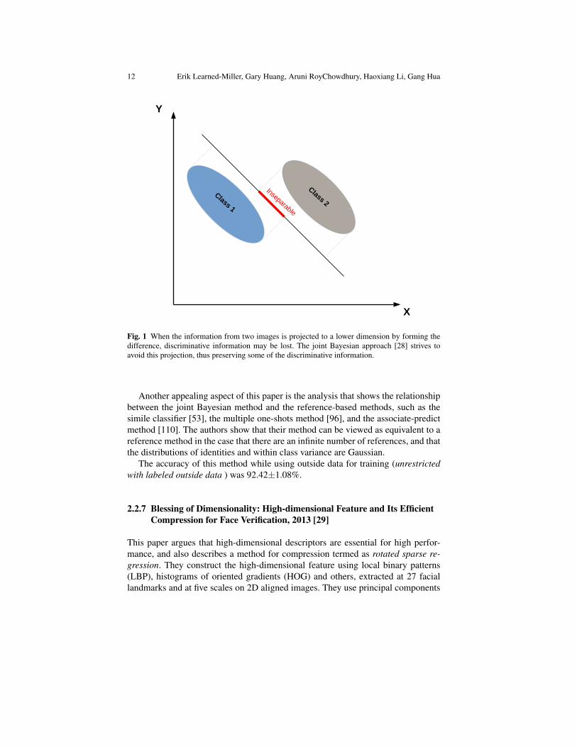
Chen et al. [28] point out a potential shortcoming of the probabilistic methodapplied to image differences. They note that by forming the image difference, infor-mation available to distinguish between two classes (in this case the “same” versus“different” classes of the verification paradigm) may be thrown out. In particular, ifx and y are two image vectors of length N, then the pair of images, considered as aconcatenation of the two vectors, contains 2N components. Forming the differenceimage is a linear operator corresponding to a projection of the image pair back to Ndimensions, hence removing some of the information that may be useful in decidingwhether the pair is “same” or “different”. This is illustrated in Figure 1. To addressthis problem, Chen et al. focus on modeling the joint distribution of image pairs(of dimension 2N) rather than the difference distribution (of dimension N). This isan elegant formulation that has had a significant impact on many of the follow-uppapers on LFW.


Class 1

Class 2

Inseparable

X

Y

Fig. 1 When the information from two images is projected to a lower dimension by forming thedifference, discriminative information may be lost. The joint Bayesian approach [28] strives toavoid this projection, thus preserving some of the discriminative information.

Another appealing aspect of this paper is the analysis that shows the relationshipbetween the joint Bayesian method and the reference-based methods, such as thesimile classifier [53], the multiple one-shots method [96], and the associate-predictmethod [110]. The authors show that their method can be viewed as equivalent to areference method in the case that there are an infinite number of references, and thatthe distributions of identities and within class variance are Gaussian.

The accuracy of this method while using outside data for training (unrestrictedwith labeled outside data ) was 92.42±1.08%.

2.2.7 Blessing of Dimensionality: High-dimensional Feature and Its EfficientCompression for Face Verification, 2013 [29]

This paper argues that high-dimensional descriptors are essential for high perfor-mance, and also describes a method for compression termed as rotated sparse re-gression. They construct the high-dimensional feature using local binary patterns(LBP), histograms of oriented gradients (HOG) and others, extracted at 27 faciallandmarks and at five scales on 2D aligned images. They use principal components


analysis (PCA) to first reduce this to 400 dimensions and use a supervised methodsuch as linear discriminant analysis (LDA) or a joint Bayesian model [28] to finda discriminative projection. In a second step, they use L1-regularized regression tolearn a sparse projection that directly maps the original high-dimensional featureinto the lower-dimensional representation learned in the previous stage.

They report accuracies of 93.18±1.07% under the unrestricted with label-freeoutside data protocol and 95.17±1.13% using their WDRef (99,773 images of 2,995subjects) data set for training following the unrestricted with labeled outside dataprotocol.

2.2.8 A Practical Transfer Learning Algorithm for Face Verification, 2013 [25]

This paper applies transfer learning to extend the high performing joint Bayesianmethod [28] for face verification. In addition to the data likelihood of the target do-main, they add the KL-divergence between the source and target domains as a reg-ularizer to the objective function. The optimization is done via closed-form updatesin an expectation-maximization framework. The source domain is the non-publicWDRef data set used in their previous versions [28, 29] and the target is set to beLFW. They use the high-dimensional LBP features from [29], reducing its size fromover 10,000 dimensions to 2,000 by PCA.

They report 96.33±1.08% accuracy on LFW in the unrestricted with labeledoutside data protocol, which improves over the results from using joint Bayesianwithout the transfer learning on high dimensional LBP features [29].

2.2.9 Hybrid Deep Learning for Face Verification, 2013 [91]

This method [91] uses an elaborate hybrid network of convolutional neural networks(CNNs) and a Classification-RBM (restricted Boltzmann machine), trained directlyfor verification. A pair of 2D aligned face images are input to the network. At thelower part, there are 12 groups of CNNs, which take in images each covering a par-ticular part of the face, some in colour and some in grayscale. Each group containsfive CNNs that are trained using different bootstrap samples of the training data. Asingle CNN consists of four convolutional layers and a max-pooling layer. Similarto [48], they use local convolutions in the mid- and high-level layers of the CNNs.There can be eight possible “input modes” or combinations of horizontally flippingthe input pair of images and each of these pairs are fed separately to the networks.The output from all these networks is in layer L0, having 8∗5∗12 neurons. The nexttwo layers average the outputs, first among the eight input modes and then the fivenetworks in a group. The final layer is a classification RBM (models the joint distri-bution of class labels, binary input vectors and binary hidden units) with two outputsthat indicate same or different class for the pairs, which is discriminatively trainedby minimizing the negative log probability of the target class given the input, usinggradient descent. The CNNs and the RBM are trained separately; then the whole


model is jointly fine-tuned using back-propagation. Model averaging is done bytraining the RBM with five different random sets of training data and averaging thepredictions. They create a new training data set, “CelebFaces”, consisting of 87,628images of 5,436 celebrities collected from the web. They report 91.75±0.48% ac-curacy on the LFW in the unrestricted with label-free outside data protocol and92.52±0.38% following the unrestricted with labeled outside data protocol.

2.2.10 POOF: Part-Based One-vs-One Features for Fine-GrainedCategorization, Face Verification, and Attribute Estimation, 2013 [17]

When annotations of parts are provided, this method learns highly discriminativefeatures between two classes based on the appearance at a particular landmark orpart that has been provided. They formulate face verification as a fine-grained clas-sification task, for which this descriptor is designed to be well suited.

For training a single “POOF” or Part-Based One-vs-One Feature, it is provided apair of classes to distinguish and two part locations - one for alignment and the otherfor feature extraction. All the images of the two classes are aligned with respectto the two locations using similarity transforms with 64 pixels horizontal distancebetween them. A crop of 64× 128 at the mid-point of the two locations is takenand grids of 8× 8 and 16× 16 are placed on it. Gradient direction histograms andcolor histograms are used as base features for each cell and concatenated. A linearsupport vector machine (SVM) is trained on these to separate the two classes. TheseSVM weights are used to find the most discriminative cell locations and a mask isobtained by thresholding these values. Starting from a given part location as a seed,its connected component is found in the thresholded mask. Base features from cellsin this connected component are concatenated and another linear SVM is used toseparate the two classes. The score from this SVM is the score of that part-basedfeature.

They learn a random subset of 10,000 POOFs using the database in [16], get-ting two 10,000-dimensional vectors for each LFW pair. They use both absolutedifference (| f (A)− f (B)|) and product ( f (A). f (B)) of these vectors to train a same-versus-different classifier on the LFW training set. They report 93.13±0.40% accu-racy on LFW following the unrestricted with labeled outside data protocol.

2.2.11 Learning Discriminant Face Descriptor for Face Recognition, 2014 [58]

This approach learned a “Discriminative Face Descriptor” (DFD) based upon im-proving the LBP feature (which are essentially differences in value of a particularpixel to its neighbours). They use the Fisher criterion for maximizing between classand minimizing within class scatter matrices to learn discriminative filters to ex-tract features at the pixel level as well as find optimal weights for the contributionof neighbouring pixels in computing the descriptor. K-means clustering is used to


find the most dominant clusters among these discriminant descriptors (typically oflength 20). They reported best performance using K=1024 or 2048.

They used the LFW-a images and cropped the images to 150×130. They furtherused a spatial grid to encode separate parts of the face separately into their DFD rep-resentation and also apply PCA whitening. The descriptors themselves were learnedusing the FERET data set (unrestricted with labeled outside data ), however the au-thors note that the distribution of images in FERET is quite different from that ofLFW – performance on LFW is an indicator of the generalizable power of theirdescriptor. They report an LFW accuracy of 84.02±0.44%.

2.2.12 Face++, 2014

We discuss two papers from the Face++/Megvii Inc. group here, both involvingsupervised deep learning on large labeled data sets. These, along with Facebook’sDeepFace [97] and DeepID[92], exploited massive amounts of labeled outside datato train deep convolutional neural networks (CNNs) and reach very high perfor-mance on LFW.

In the first paper from the Face++ group, a new structure, which they term thepyramid CNN [34] is used. It conducts supervised training of a deep neural net-work one layer at a time, thus greatly reducing computation. A four-level Siamesenetwork trained for verification was used. The network was applied on four facelandmarks and the outputs were concatenated. They report an accuracy of 97.3% onthe LFW unrestricted with labeled outside data protocol.

The Megvii Face Recognition System [113] was trained on a data set of 5 millionlabeled faces of around 20,000 identities. A ten-layer network was trained for iden-tification on this data set. The second-to-last layer, followed by PCA, was used asthe face representation. Face verification was done using the L2 norm score, achiev-ing 99.50±0.36% accuracy. With the massive training data set size, they argue thatthe advantages of using more sophisticated architectures and methods become lesssignificant. They investigate the long tail effect of web-collected data (lots of per-sons with very few image samples) and find that after the first 10,000 most frequentindividuals, including more persons with very few images into the training set doesnot help. They also show in a secondary experiment that high performance on LFWdoes not translate to equally high performance in a real-world security certificationsetting.

2.2.13 DeepFace: Closing the Gap to Human-Level Performance in FaceVerification, 2014 [97]

This paper from Facebook [97] has two main novelties - a method for 3D facefrontalization7 and a deep neural net trained for classification. The neural network

7 See Section 3 for a discussion of previous work on 3D frontalization.


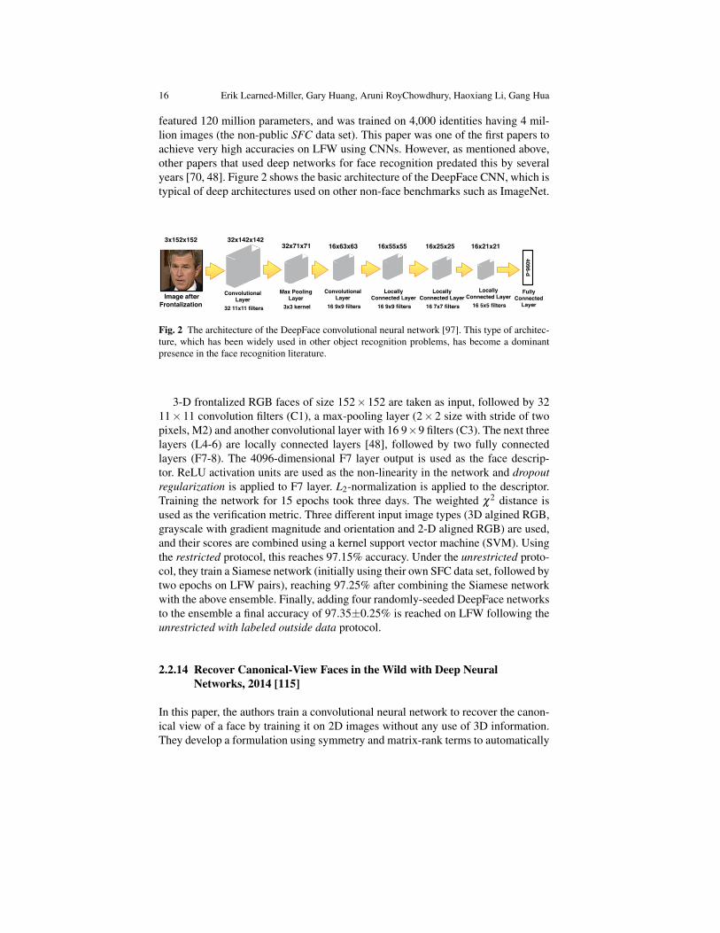
featured 120 million parameters, and was trained on 4,000 identities having 4 mil-lion images (the non-public SFC data set). This paper was one of the first papers toachieve very high accuracies on LFW using CNNs. However, as mentioned above,other papers that used deep networks for face recognition predated this by severalyears [70, 48]. Figure 2 shows the basic architecture of the DeepFace CNN, which istypical of deep architectures used on other non-face benchmarks such as ImageNet.

Image after Frontalization

3x152x152

32 11x11 filters

ConvolutionalLayer

3x3 kernel

Max PoolingLayer

16 9x9 filters

ConvolutionalLayer

16 9x9 filters

Locally Connected Layer

16 7x7 filters


16 5x5 filters


4096-d

Fully Connected

Layer

32x142x14232x71x71 16x63x63 16x55x55 16x25x25 16x21x21

Fig. 2 The architecture of the DeepFace convolutional neural network [97]. This type of architec-ture, which has been widely used in other object recognition problems, has become a dominantpresence in the face recognition literature.

3-D frontalized RGB faces of size 152×152 are taken as input, followed by 3211×11 convolution filters (C1), a max-pooling layer (2×2 size with stride of twopixels, M2) and another convolutional layer with 16 9×9 filters (C3). The next threelayers (L4-6) are locally connected layers [48], followed by two fully connectedlayers (F7-8). The 4096-dimensional F7 layer output is used as the face descrip-tor. ReLU activation units are used as the non-linearity in the network and dropoutregularization is applied to F7 layer. L2-normalization is applied to the descriptor.Training the network for 15 epochs took three days. The weighted χ2 distance isused as the verification metric. Three different input image types (3D algined RGB,grayscale with gradient magnitude and orientation and 2-D aligned RGB) are used,and their scores are combined using a kernel support vector machine (SVM). Usingthe restricted protocol, this reaches 97.15% accuracy. Under the unrestricted proto-col, they train a Siamese network (initially using their own SFC data set, followed bytwo epochs on LFW pairs), reaching 97.25% after combining the Siamese networkwith the above ensemble. Finally, adding four randomly-seeded DeepFace networksto the ensemble a final accuracy of 97.35±0.25% is reached on LFW following theunrestricted with labeled outside data protocol.

2.2.14 Recover Canonical-View Faces in the Wild with Deep NeuralNetworks, 2014 [115]

In this paper, the authors train a convolutional neural network to recover the canon-ical view of a face by training it on 2D images without any use of 3D information.They develop a formulation using symmetry and matrix-rank terms to automatically


select the frontal face image for each person at training time. Then the deep networkis used to learn the regression from face images in arbitrary view to the canonical(frontal) view.

After this canonical pose recovery is performed, they detect five landmarks fromthe aligned face and train a separate network for each patch at each landmark alongwith one network for the entire face. These small networks (two convolutional andtwo pooling layers) are connected at the fully connected layer and trained on theCelebFaces data set [91] with the cross-entropy loss to predict identity labels. Fol-lowing this, a PCA reduction is done, and an SVM is used for the verification task,resulting in an accuracy of 96.45±0.25% under the unrestricted with labeled outsidedata protocol.

2.2.15 Deep Learning Face Representation from Predicting 10,000 Classes,2014 [92]

In this approach, called “DeepID” [92], the authors trained a network to recognize10,000 face identities from the “CelebFaces” data set [91] (87,628 face images of5436 celebrities, non-overlapping with LFW identities). The CNNs had four convo-lutional layers (with 20, 40, 60 and 80 feature maps), followed by max-pooling, a160-dimensional fully-connected layer (DeepID-layer) and a softmax layer for theidentities. The higher convolutional layers had locally shared weights. The fully-connected layer was connected to both the third and fourth convolutional layers inorder to see multi-scale features, referred to as a “skipping” layer. Faces were glob-ally aligned based on five landmarks. The input to a network was one out of 60patches, which were square or rectangular and could be both colour or grayscale.Sixty CNNs were trained on flipped patches, yielding a 160∗2∗60 dimensional de-scriptor of a single face. PCA reduction to 150 dimensions was done before learningthe joint Bayesian model, reaching an accuracy of 96.05%. Expanding the data set(CelebFaces+ [88]) and using the joint Bayesian model for verification gives them afinal accuracy of 97.45±0.26% under the unrestricted with labeled outside data pro-tocol.

2.2.16 Surpassing Human-Level Face Verification Performance on LFW withGaussianFace, 2014 [65]

This method uses multi-task learning and the discriminative Gaussian process la-tent variable model (DGP-LVM) [55, 100] to be one of the top performers onLFW. The DGP-LVM [100] maps a high-dimensional data representation to a lower-dimensional latent space using a discriminative prior on the latent variables whilemaximizing the likelihood of the latent variables in the Gaussian process (GP)framework for classification. GPs themselves have been observed to be able to makeaccurate predictions given small amounts of data [55] and are also robust to situa-tions when the training and test data distributions are not identical. The authors


were motivated to use DGP-LVM over the more usual GPs for classifications as theformer, by virtue of its discriminative prior, is a more powerful predictor.

The DGP-LVM is reformulated using a kernelized linear discriminant analysisto learn the discriminative prior on latent variables and multiple source domainsare used to train for the target domain task of verification on LFW. They detailtwo uses of their Gaussian Face model - as a binary classifier and as a featureextractor. For the feature extraction, they use clustering based on GPs [51] on thejoint vectors of two faces. They compute first and second order statistics for inputjoint feature vectors and their latent representations and concatenate them to formthe final feature. These GP-extracted features are used in the GP-classifier in theirfinal model.

Using 200,000 training pairs, the “GaussianFace” model reached 98.52±0.66%accuracy on LFW under the unrestricted with labeled outside data protocol, sur-passing the recorded human performance on close-cropped faces (97.53%).

2.2.17 Deep Learning Face Representation by JointIdentification-Verification, 2014 [88]

Building on the previous model, DeepID [92], “DeepID2” [88] used both an iden-tification signal (cross-entropy loss) and a verification signal (L2 norm verificationloss between DeepID2 pairs) in the objective function for training the network, andexpanded the CelebFaces data set to “CelebFaces+”, which has 202,599 face imagesof 10,177 celebrities from the web. 400 aligned face crops were taken to train a net-work for each patch and a greedy selection algorithm was used to select the best 25of these. A final 4000 (25*160) dimensional face representation was obtained, fol-lowed by PCA reduction to 180-dimensions and joint Bayesian verification, achiev-ing 98.97% accuracy.

The network had four convolutional layers and max-pooling layers were usedafter the first three convolutional layers. The third convolutional layer was locallyconnected, sharing weights in 2× 2 local regions. As mentioned before, the lossfunction was a combined loss from identification and verification signals. The ratio-nale behind this was to encourage features that can discriminate identity, and alsoreduce intra-personal variations by using the verification signal. They show that us-ing either of the losses alone to train the network is sub-optimal and the appropriateloss function is a weighted combination of the two.

A total of seven networks are trained using different sets of selected patchesfor training. The joint Bayesian scores are combined using an SVM, achieving99.15±0.13% accuracy under the unrestricted with labeled outside data protocol.


2.2.18 Deeply Learned Face Representations are Sparse, Selective andRobust, 2014 [93]

Following on with the DeepID “family” of models, “DeepID2+” [93] increased thenumber of feature maps to 128 in the four convolutional layers, the DeepID sizeto 512 dimensions and expanded their training set to around 290,000 face imagesfrom 12,000 identities by merging the CelebFaces+ [88] and WDRef [29] data sets.Another interesting novelty of this method was the use of a loss function at multiplelayers of the network, instead of the standard supervisory signal (loss function) inthe top layer. They branched out 512-dimensional fully-connected layers at each ofthe 4 convolutional layers (after the max-pooling step) and added the loss function(a joint identification-verification loss) after the fully-connected layer for additionalsupervision at the early layers. They show that removal of the added supervisionlowers their performance, as well as some interesting analysis on the sparsity ofthe neural activations. They report that only about half the neurons get activatedfor an image, and each neuron activates for about half the images. Moreover theyfound a difference of less than 1% when using a binary representation by threshold-ing, which led them to state that the fact that a neuron is activated or not is moreimportant than the actual value of that activation.

This report an accuracy of 99.47±0.12% (unrestricted with labeled outside data )using the joint Bayesian model trained on 2000 people in their training set and com-bining the features from 25 networks trained on the same patches as DeepID2 [88].

2.2.19 DeepID3: Face Recognition with Very Deep Neural Networks, 2015 [89]

“DeepID3” uses a deeper network (10 to 15 feature extraction layers) with Inceptionlayers [94] and stacked convolution layers (successive convolutional layers with-out any pooling layer in between) on a similar overall pipeline to DeepID2+ [93].Similar to DeepID2+, they include unshared weights in later convolutional layers,max-pooling in early layers and the addition of joint identification-verification lossfunctions to branched-out fully connected layers from each pooling layer in the net-work.

They train two networks, one using the stacked convolution and the other usingthe recently-proposed Inception layer used in the GoogLeNet architecture, whichwas a top-performer in the ImageNet challenge in 2015 [94]. The two networksreduce the error rate of DeepID2+ by 0.81% and 0.26%, respectively.

The features from both the networks on 25 patches is combined into a vectorof about 30,000 dimensions. It is PCA reduced to 300 dimensions, followed bylearning a joint Bayesian model. It achieved 99.53±0.10% verification accuracy onLFW (unrestricted with labeled outside data ).


2.2.20 FaceNet: A unified embedding for face recognition and clustering,2015 [82]

This model from Google, called the FaceNet [82], uses 128-dimensional represen-tations from very deep networks, trained on a 260-million image data set using atriplet loss at the final layer - the loss separates a positive pair from a negative pairby a margin. An online hard negative exemplar mining strategy within each mini-batch is used in training the network. This loss directly optimizes for the verificationtask and so a simple L2 distance between the face descriptors is sufficient.

They use two variants of networks. In NN1, they add 1×1×d convolutional lay-ers between the standard Zeiler&Fergus CNN [112] resulting in 22 layers. In NN2,they use the recently proposed Inception modules from GoogLeNet [94] which ismore efficient and has 20 times lesser parameters. The L2-distance threshold forverification is estimated from the LFW training data. They report results, follow-ing the unrestricted with labeled outside data protocol, on central crops of LFW(98.87±0.15%) and when using a proprietary face detector (99.6±0.09%) using theNN1 model, which is the highest score on LFW in the unrestricted with labeledoutside data protocol. The scores from using the NN2 model were reported to bestatistically in the same range.

2.2.21 Tencent-BestImage, 2015 [8]

This commercial system followed the unrestricted with labeled outside data pro-tocol and built their system combining an alignment system, a deep convolutionalneural network with 12 convolution layers, and the joint Bayesian method for ver-ification. The whole system was trained on their data set - “BestImage CelebritiesFace” (BCF), which contains about 20,000 individuals and 1 million face imagesand is identity-disjoint with respect to LFW. They divided the BCF data into twosubsets for training and validation. The network was trained on the BCF training setwith 20 face patches. The features from each patch were concatentated, followedby PCA and the joint Bayesian model learned on BCF validation set. They reportan accuracy of 99.65±0.25% on LFW under the unrestricted with labeled outsidedata protocol.

2.3 Label-free outside data protocols

In this section, we discuss two of the LFW protocols together–image-restricted withlabel-free outside data and unrestricted with label-free outside data. While theseresults are curated separately for fairness on the LFW page, conceptually they arehighly similar, and are not worth discussing separately.

These protocols allow the use of outside data such as additional faces, landmarkannotations, part labels, and pose labels, as long as this additional information does


Method Net. Loss Outside data # models Aligned Verif. metric Layers Accu.DeepFace [97] ident. 4M 4 3D wt. chi-sq. 8 97.35±0.25

Canon. view CNN [115] ident. 203K 60 2D Jt. Bayes 7 96.45±0.25DeepID [92] ident. 203K 60 2D Jt. Bayes 7 97.45±0.26DeepID2 [88] ident. + verif. 203K 25 2D Jt. Bayes 7 99.15±0.13

DeepID2+ [93] ident. + verif. 290K 25 2D Jt. Bayes 7 99.47±0.12DeepID3 [89] ident. + verif. 290K 25 2D Jt. Bayes 10-15 99.53±0.10Face++ [113] ident. 5M 1 2D L2 10 99.50±0.36FaceNet [82] verif. (triplet) 260M 1 no L2 22 99.60±0.09Tencent [8] - 1M 20 yes Jt. Bayes 12 99.65±0.25

Table 2 CNN top results: As some of the highest results on LFW have been from using supervisedconvolutional neural networks (CNNs), we compare the details of the top-performing CNN meth-ods in a separate table. N.B. – unknown parameters that were not mentioned in the correspondingpapers are denoted with a “-”.

not contain any information that would allow making pairs of images labeled “same”or “different”. For example, a set of images of a single person (even if the personwere not labeled) or a video of a person would not be allowed under these protocols,since any pair of images from the set or from the video would allow the formationof a “same” pair.

Still, large amounts of information can be used by these methods to understandthe general structure of the space of faces, to build supervised alignment methods,to build attribute classifiers, and so on. Thus, these methods would be expected tohave a significant advantage over the “no outside data” protocols.

2.3.1 Face recognition using boosted local features, 2003 [50]

One of the earliest methods applied to LFW was developed at Mitsubishi ElectricResearch Labs (MERL) by Michael Jones and Paul Viola [50]. This work built onthe authors’ earlier work in boosting for face detection [101], adapting it to learna similarity measure between face images using a modified AdaBoost algorithm.They use filters that act on a pair of images as features, which are a set of linearfunctions that are a superset of the “rectangle” filters used in their face detectionsystem. A threshold on the absolute difference of the scalar values returned by afilter applied on a pair of faces can be used to determine valid or invalid variation ofa particular property or aspect of a face (the validity being with respect to whetherthe faces belong to the same identity).

The technical report was released before LFW, and so does not describe appli-cation to the database, but the group submitted results on LFW after publication,achieving 70.52±0.60%.


2.3.2 LFW Results Using a Combined Nowak Plus MERL Recognizer, 2008[46]

This early system combined the method of Nowak et al. [74] with an unpublishedmethod [46] from Mitsubishi Electric Research Laboratory (MERL), and thus tech-nically counts as a method whose full details are not published. However, somedetails are given in a workshop paper [46].

The MERL system initially detects a face using a Viola-Jones frontal face de-tector, followed by alignment based on nine facial landmarks (also detected usinga Viola-Jones detector). After alignment, some simple lightning normalization isdone. The score of the MERL face recognition system [50] is then averaged withthe score from the best-performing system of that time (2007), by Nowak and Ju-rie [74].

The accuracy of this system was 76.18±0.58%.

2.3.3 Is that you? Metric Learning Approaches for Face Identification, 2009[39]

This paper presents two methods to learn robust distance measures for face veri-fication, the logistic discriminant-based metric learning (LDML) and marginalizedK–nearest neighbors (MkNN) classifier. The LDML learns a Mahalanobis distancebetween two images to make the distances between positive pairs smaller than thedistances between negative pairs and obtain a probability that a pair is positive in astandard linear logistic discriminant model. The MkNN classifies an image pair be-longs to the same class with the marginal probability that both of them are assignedto the same class using a k–nearest neighbor classifier. In the experiments, theyrepresent the images as stacked multi-scale local descriptors extracted at nine faciallandmarks. The facial landmarks detector is trained with outside data. Without usingthe identify labels for the LFW training data, the LDML achieves 79.27±0.6% un-der the image-restricted with label-free outside data protocol. They obtain this accu-racy by fusing the scores from eight local features including LBP, TPLBP, FPLBP,SIFT and their element-wise square root variants with a linear combination. Thismultiple feature fusion method is shown to be effective in a number of literatures.Under the unrestricted with label-free outside data protocol, they show that the per-formance of LDML is significantly improved with more training pairs formed usingthe identity labels. And they obtain their best performance 87.50± 0.4% accuracyby linearly combining the 24 scores with the three methods LDML, large marginnearest neighbor (LMNN) [102] and MkNN over the eight local features.

2.3.4 Multiple One-Shots for Utilizing Class Label Information, 2009 [96]

The authors extend the one-shot similarity (OSS) introduced in [104] which wewill describe under the image-restricted, no outside data protocol. In brief, the OSS


for an image pair is obtained by training a binary classifier with one image in thepair as the positive sample and a set of pre-defined negative samples to classifythe other image in the pair. This paper extends the OSS to be multiple one-shotssimilarity vector by producing OSS scores with different negative sample sets. Eachset reflecting either a different subject or a different pose. In their face verificationsystem, the faces are firstly aligned with a commercial face alignment system. Thealigned faces are published as the “aligned” LFW data set or LFW-a data set. Theface descriptors are then constructed by stacking local descriptors extracted denselyover the face images. The information theoretic metric learning (ITML) methodis adopted to obtain a Mahalanobis matrix to transform the face descriptors and alinear SVM classifies a pair of faces to be matched or not based on the multipleOSS scores. They achieve their best result 89.50± 0.51% accuracy by combining16 multiple OSS scores including eight descriptors (SIFT, LBP, TPLBP, FPLBPand their square root variants) under two settings of the multiple OSS scores (thesubject-based negative sample sets and pose-based negative sample sets).

2.3.5 Attribute and Simile Classifiers for Face Verification. 2009 [53]

We discussed the attribute and simile classifiers for face verification [53] under theunrestricted with labeled outside data protocol. The authors’ result with the attributeclassifier qualifies for the unrestricted with label-free outside data protocol. Theyreported their result with the attribute classifier on LFW as 85.25±0.60% accuracyin their follow-up journal paper [54].

2.3.6 Similarity Scores based on Background Samples, 2010 [105]

In this paper, Wolf et al. [105] extend the one-shot similarity (OSS) introducedin [104] to the two-shot similarity (TSS). The TSS score is obtained by training aclassifier to classify the two face images in a pair against a background face set. Al-though the TSS score by itself is not discriminative for face verification, they showthat the performance is improved by combining the TSS scores with OSS scores andother similarity scores. They extend the OSS and TSS framework to use linear dis-criminant analysis instead of an SVM as the online trained classifier. In addition toOSS and TSS, they propose to represent each image in the pair with its rank vectorobtained by retrieving similar images from the background face set. The correla-tion between the two rank vectors provides another dimensionality of the similaritymeasure of the face pair. In their experiments, they use the LFW-a data set to handlealignment. Combining the similarities introduced above with eight variants of localdescriptors, they obtain an accuracy of 86.83± 0.34% under the image-restrictedwith label-free outside data protocol.


2.3.7 Rectified Linear Units Improve Restricted Boltzmann Machines, 2010[70]

Restricted Boltzmann machines (RBMs) are often formulated as having binary-valued units for the hidden layer and Gaussian units for the real-valued input layer.Nair and Hinton [70] modify the hidden units to be “noisy rectified linear units”(NReLUs), where the value of a hidden unit is given by the rectified output of theactivation and some added noise, i.e. max(0,x+N(0,V )), where x is the activation ofthe hidden unit given an input, and N(0,V ) is the Gaussian noise. RBMs with 4000NReLU units in the hidden layer are first pre-trained generatively, then discrimina-tively trained as a feed-forward fully-connected network using back-propagation (inthe latter case the Gaussian noise term is dropped in the rectification).

In order to model face pairs, they use a “Siamese” network architecture, wherethe same network is applied to both faces and the cosine distance is the symmetricfunction that combines the two outputs of the network. They show that that NRe-LUs are translation equivariant and scale equivariant(the network outputs changein the same way as the input), and combined with the scale invariance of cosinedistance the model is analytically invariant to the rescaling of its inputs. It is nottranslation invariant. LFW images are center-cropped to 144× 144, aligned basedon the eye location and sub-sampled to 32× 32 3-channel images. Image intensi-ties are normalized to be zero-mean and unit-variance. They report an accuracy of80.73±1.34% (image-restricted with label-free outside data ). It should be notedthat because the authors use manual correction of alignment errors, this paper doesnot conform to the LFW protocols, and thus need not be used as a comparisonagainst fully automatic methods.

2.3.8 Face Recognition with Learning-based Descriptor, 2010 [26]

This paper was discussed under the unrestricted with labeled outside data protocol.With the holistic face as the only component, the method qualifies for the image-restricted with label-free outside data protocol, under which the authors obtain anaccuracy of 81.22±0.35%.

2.3.9 Cosine Similarity Metric Learning for Face Verification, 2011 [72]

This paper proposes cosine similarity metric learning (CSML) to learn a transforma-tion matrix to project faces into a subspace in which cosine similarity performs wellfor verification. They define the objective function to maximize the margin betweenthe cosine similarity scores of positive pairs and cosine similarity scores of negativepairs while regularizing the learned matrix by a predefined transformation matrix.They empirically demonstrate that this straightforward idea works well on LFWand that by combining scores from six different feature descriptors their methodachieves an accuracy of 88.00± 0.38% under the image-restricted with label-free


outside data protocol. Subsequent communication with the authors revealed an errorin the use of the protocol. Had the protocol been followed properly, our experimentssuggest that the results would be about three percent lower, i.e., about 85%. Still,this method has played an important role in subsequent research as a popular choicefor the comparison of feature vectors.

2.3.10 Beyond Simple Features: A Large-Scale Feature Search Approach toUnconstrained Face Recognition, 2011 [31]

This method [31] uses the biologically-inspired V1-like features that are designedto approximate the initial stage of the visual cortex of primates. It is essentially acascade of linear and non-linear functions. These are stacked into two and threelayer architectures, HT-L2 and HT-L3 respectively. These models take in 100×100and 200× 200 grayscale images as inputs. A linear SVM is trained on a varietyof vector comparison functions between two face descriptors. Model selection isdone on 5,915 HT-L2 and 6,917 HT-L3 models before the best five were selected.Multiple kernels were used to combine data augmentations (rescaled crops of 250×250, 150× 150 and 125× 75), blend the top five models within each “HT class”,and also blend models across HT classes. The HT-L3 gives an accuracy of 87.8%while combining all of the models gives a final accuracy of 88.13±0.58% followingthe image-restricted with label-free outside data protocol.

2.3.11 Face Verification Using the LARK Representation, 2011 [84]

This work extends previous work [83] in which two images are represented as twolocal feature sets and the matrix cosine similarity (MCS) is used to separate facesfrom backgrounds. All kinds of visual variations are addressed implicitly in theMCS which is the weighted sum of the cosine similarities of the local features. Inthis work, the authors present the locally adaptive regression kernel (LARK) localdescriptor for face verification. LARK is defined as the self-similarity between acenter pixel and its surroundings. In particular, the distance between two pixels isthe geodesic distance. They consider an image as a 3D space which includes the2D coordinates and the gray-scale value at each pixel. The geodesic distance isthen the shortest path on the image surface. PCA is then adopted to reduce thedimensionality of the local features. They further apply an element-wise logisticfunction to generate a binary-like representation to remove the dominance of largerelative weights to increase the discriminative power of the local features. Theyconduct experiments on LFW under both the unsupervised protocol and the imagerestricted protocol.

In the unsupervised setting, they compute LARKs of size 7× 7 from each faceimage. They evaluate various combinations of different local descriptors and simi-larity measures and report that the LBP with Chi-square distance achieves the best69.54% accuracy among the baseline methods. Their method achieves 72.23% ac-


curacy. Under the image-restricted with label-free outside data protocol, they adoptthe OSS with LDA for face verification and achieve an accuracy of 85.10±0.59%by fusing scores from 14 combinations of local descriptors (SIFT, LBP, TPLBP andpcaLARK) and similarity measures (OSS, OSS with logistic function, MCS andMCS with logistic function).

2.3.12 Probabilistic Models for Inference About Identity, 2012 [62]

This paper presents a probabilistic face recognition method. Instead of representingeach face as a feature vector and measuring the distances between faces in the fea-ture space, they propose to construct a model in which identity is a hidden variablein a generative description of the image data. Other variations in pose, illumina-tion and etc., is described as noise. The face recognition is then framed as a modelcomparison task.

More concretely, they present a probabilistic latent discriminant analysis (PLDA)model to describe the data generation. In PLDA, the data generation depends on thelatent identity variable and an intra-class variation variable. This design helps fac-torize the identity subspace and within-individual subspace. The model is learnedby expectation-maximization (EM) and the face verification is conducted by look-ing at the likelihood ratio of an image pair generated by a similar pair model overa dissimilar pair model. The PLDA model is further extended to be a mixture ofPLDA models to describe the potential non-linearity of the face manifold. Extensiveexperiments are conducted to evaluate the PLDA and its variants in face analysis.Their face verification result on LFW is 90.07±0.51% under the unrestricted withlabel-free outside data protocol.

2.3.13 Large Scale Strongly Supervised Ensemble Metric Learning, withApplications to Face Verification and Retrieval, 2012 [43]

High-dimensional overcomplete representations of data are usually informative butcan be computationally expensive. This paper proposes a two-step metric learningmethod to enforce sparsity and to avoid features with little discriminability and im-prove computational efficiency. The two-step design is motivated by the fact thatstraightforwardly applying the group lasso with row-wise and column-wise L1 reg-ularization is very expensive in high-dimensional feature spaces. In the first step,they iteratively select µ groups of features. In each iteration, the feature group whichgives the largest partial derivative of the loss function is chosen and the Mahalanobismatrix of a weak metric for the selected feature group is learned and assembled intoa sparse block diagonal matrix A†. With an eigenvalue decomposition, they obtain atransformation matrix to reduce the feature dimensionality. After that, in the secondstep, another Mahalanobis matrix is learned to exploit the correlations between theselected feature groups in the lower-dimensional subspace. They adopt the projectedgradient descent method to iteratively learn the Mahalanobis matrix.


In their experiments, they use the LFW-a data set and center crop the face imagesto 110×150. By concatenating two types of features (covariance matrix descriptorsand soft local binary pattern histograms) after the first step, they achieve 92.58±1.36% accuracy under the image-restricted with label-free outside data protocol.

2.3.14 Distance Metric Learning with Eigenvalue Optimization, 2012 [111]

In this paper, the authors present an eigenvalue optimization framework for learninga Mahalanobis metric. They learn the metric by maximizing the minimal squareddistances between dissimilar pairs while maintaining an upper bound for the sum ofsquared distances between similar pairs. They further show that this is equivalent toan eigenvalue optimization problem. Similarly, the previous metric learning methodLMNN can also be formulated as a general eigenvalue decomposition problem.

They further develop an efficient algorithm to solve this optimization problem,which will only involve the computation of the largest eigenvector of a matrix. In theexperiments, they show that the proposed method is more efficient than other metriclearning methods such as LMNN and ITML. On LFW, they evaluate this methodwith both the LFW funneled data set and the LFW-a data set. They use SIFT featurescomputed at the fiducial points for faces on the funneled LFW data set and achieve81.27±2.30% accuracy. On the “aligned” LFW data set, they evaluate three types offeatures including concatenated raw intensity values, LBP and TPLBP. Combiningthe scores from the four different features with a linear SVM, they achieve 85.65±0.56% accuracy under the image-restricted with label-free outside data protocol.

2.3.15 Learning Hierarchical Representations for Face Verification withConvolutional Deep Belief Networks, 2012 [48]

In this work [48], a local convolutional deep belief network is used to generativelymodel the distribution of faces. Then, a discriminatively learned metric (ITML) isused for the verification task. The shared weights of convolutional filters (10× 10in size) in the CRBM (convolutional RBM) makes it possible to use high-resolutionimages as input. Probabilistic max-pooling is used in the CRBM to have local trans-lation invariance and still allow top-down and bottom-up inference in the model.

The authors argue that in images like faces, that exhibit clear spatial structure,the weights of a hidden unit being shared across the locations in the whole imageis not desirable. On the other hand, using a layer with fully-connected weights maynot be computationally tractable without either subsampling the input image or firstapplying several pooling layers. In order to exploit this structure, the image is di-vided into overlapping regions and the weight-sharing in the CRBM is restricted tobe local. Contrastive divergence is used to train the local CRBM. Two layers of theseCRBMs are stacked to form a deep belief network (DBN). The local CRBM is usedin the second layer of their network. In addition to using raw pixels, the uniformLBP descriptor is also used as input to the DBN. The two features are combined at


the score level by using a linear SVM. The LFW-a face images are used as input,with three croppings at sizes 150×150,125×75,100×100, resized to the same sizebefore input to the DBN. The deep learned features give competitive performance(86.88±0.62%) to hand-crafted features (87.18±0.49%), while combining the twogives the highest of 87.77±0.62% (image-restricted with label-free outside data ).

2.3.16 Bayesian Face Revisited: A Joint Formulation, 2012 [28]

We discussed this paper under the unrestricted with labeled outside data proto-col. The authors also present their result under the unrestricted with label-free out-side data protocol. Combining scores of four descriptors (SIFT, LBP, TPLBP andFPLBP), they achieve an accuracy of 90.90±1.48% on LFW.

2.3.17 Blessing of Dimensionality: High-dimensional Feature and Its EfficientCompression for Face Verification, 2013 [29]

We discussed this paper under the unrestricted with labeled outside data protocol.Without using the WDRef data set for training, they report an accuracy of 93.18±1.07% under the unrestricted with label-free outside data protocol.

2.3.18 Fisher Vector Faces in the Wild, 2013 [85]

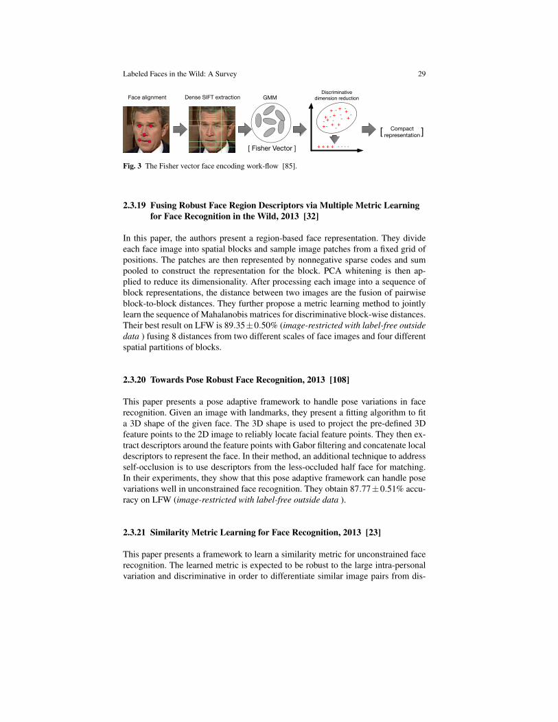
In this paper, Simonyan et al. [85] adopt the Fisher vector (FV) for face verification.The FV encoding had been shown to be effective for general object recognition.This paper demonstrates that this encoding is also effective for face recognition. Toaddress the potential high computational expense due to the high dimensionality ofthe Fisher vectors, the authors propose a discriminative dimensionality reduction toproject the vectors into a low dimensional subspace with a linear projection.

To encode a face image with FV, it is first processed into a set of densely extractedlocal features. In this paper, the dense local feature of an image patch is the PCA-SIFT descriptor augmented by the normalized image patch location in the image.They train a Gaussian mixture model (GMM) with diagonal covariance over allthe training features. As shown in Figure 3, to encode a face image with FV, theface image is first aligned with respect to the fiducial points. The Fisher vector isthen the stacked, average first and second order differences of the image featuresover each GMM component center. To construct a compact and discriminative facerepresentation, the authors propose to adopt a large-margin dimensionality reductionstep after the Fisher vector encoding.

In their experiments, they report their best result as 93.03± 1.05% accuracy onLFW under the unrestricted with label-free outside data protocol.


Face alignment Dense SIFT extraction GMM

[ Fisher Vector ]

Discriminativedimension reduction

+ ++++

++++

+

--- --- -

-

--

+ + + + - - - -

Compact representation[ ]

Fig. 3 The Fisher vector face encoding work-flow [85].

2.3.19 Fusing Robust Face Region Descriptors via Multiple Metric Learningfor Face Recognition in the Wild, 2013 [32]

In this paper, the authors present a region-based face representation. They divideeach face image into spatial blocks and sample image patches from a fixed grid ofpositions. The patches are then represented by nonnegative sparse codes and sumpooled to construct the representation for the block. PCA whitening is then ap-plied to reduce its dimensionality. After processing each image into a sequence ofblock representations, the distance between two images are the fusion of pairwiseblock-to-block distances. They further propose a metric learning method to jointlylearn the sequence of Mahalanobis matrices for discriminative block-wise distances.Their best result on LFW is 89.35±0.50% (image-restricted with label-free outsidedata ) fusing 8 distances from two different scales of face images and four differentspatial partitions of blocks.

2.3.20 Towards Pose Robust Face Recognition, 2013 [108]

This paper presents a pose adaptive framework to handle pose variations in facerecognition. Given an image with landmarks, they present a fitting algorithm to fita 3D shape of the given face. The 3D shape is used to project the pre-defined 3Dfeature points to the 2D image to reliably locate facial feature points. They then ex-tract descriptors around the feature points with Gabor filtering and concatenate localdescriptors to represent the face. In their method, an additional technique to addressself-occlusion is to use descriptors from the less-occluded half face for matching.In their experiments, they show that this pose adaptive framework can handle posevariations well in unconstrained face recognition. They obtain 87.77±0.51% accu-racy on LFW (image-restricted with label-free outside data ).

2.3.21 Similarity Metric Learning for Face Recognition, 2013 [23]

This paper presents a framework to learn a similarity metric for unconstrained facerecognition. The learned metric is expected to be robust to the large intra-personalvariation and discriminative in order to differentiate similar image pairs from dis-


similar image pairs. The robustness is introduced by projecting the face representa-tions into the intra-personal subspace, which is spanned by the top eigenvectors ofthe intra-personal covariance matrix after the whitening process. After mapping theimages to the intra-personal subspace, the discrimination is incorporated in learn-ing the similarity metric. The similarity metric is defined as the difference of theimage pair similarity against the distance measure, parameterized by two matricesrespectively. The matrices are learned by minimizing the hinge loss and regulariz-ing the two matrices to identity matrices. In their experiments, they use LBP andTBLBP descriptors on the LFW-a data set and SIFT descriptors on the LFW fun-neled data set computed at nine facial key points. Under the image-restricted withlabel-free outside data protocol, combining six scores from the three descriptorsand their square roots variants they achieve 89.73±0.38% accuracy. Under the un-restricted with label-free outside data protocol, they generate more training pairswith the identity labels and improve the accuracy to 90.75±0.64%.

2.3.22 Fast High Dimensional Vector Multiplication Face Recognition, 2013[12]

In this method, the authors propose the over-complete LBP (OCLBP) descriptor,which is the concatenation of LBP descriptors extracted with different block andradius sizes. The OCLBP based face descriptor is then processed by Whiten-PCAand LDA. They further introduce a non-linear dimensionality reduction techniqueDiffusion Maps (DM) with the proposed framework. Extensive experiments are con-ducted with different local features and dimensionality reduction methods combina-tions. They report 91.10± 0.59% accuracy under the image-restricted with label-free outside data protocol and 92.05±0.45% under the unrestricted with label-freeoutside data protocol.

2.3.23 Discriminative deep metric learning for face verification in the wild,2014 [41]

In this method, referred to as DDML, a verification loss between pairs of faces isdirectly incorporated into a deep neural network, resulting in a non-linear distancemetric that can be trained end-to-end using the back-propagation algorithm. Therationale for the verification loss is that the squared Euclidean distance betweenpositive pairs is smaller than that between negative pairs, formulated as a large mar-gin metric learning problem. The network is initialized randomly with three layersand tanh as the nonlinear activation function. They use 80×150 crops of the LFW-a(aligned) data set and extract Dense SIFT (45 SIFT descriptors from 16× 16 non-overlapping patches, resulting in a 5760-dimensional vector), LBP features (10×10non-overlapping blocks to get a 7080-dimensional vector) and Sparse SIFT (SIFTcomputed on 9 fixed landmarks at 3 scales on the funneled LFW images, resulting ina 3456-dimensional vector). These features are projected down to 500 dimensions


using PCA Whitening. Multiple features are fused at the score level by averag-ing. Their final accuracy is 90.68±1.41% (image-restricted with label-free outsidedata ).

2.3.24 Large Margin Multi-Metric Learning for Face and KinshipVerification in the Wild, 2014 [42]

In this paper, a large margin multi-metric learning (LM3L) method is proposed toexploit discriminative information from multiple features of the same face image.Extracting multiple features from the face images, the distance between two faceimages is the weighted sum of Mahalanobis distances in each image feature. LM3Ljointly learn the distance metrics in different features and the weights of the featuresby optimizing each distance metric to be discriminative while minimizing the dif-ference of distances in different features of the same image pair. They evaluate themethod on the LFW-a data set with SIFT, LBP and Sparse SIFT features. With allthe features, they achieve an accuracy of 89.57±1.53% under the image-restrictedwith label-free outside data protocol.

2.3.25 Effective Face Frontalization in Unconstrained Images, 2014 [40]

To show the importance of 3D frontalization to the task of face verification, in thispaper Hassner et al. [40] evaluate their alignment technique using an earlier facerecognition method [104], so that the impact of 3D alignment is not subsumed bythe representation power of a more powerful model like the deep network.

Prior work in 3D frontalization of faces [97] would try to reconstruct the 3Dsurface of a face and then use this 3D model to general views, usually of a canoni-cal pose. This paper explores the alternative of using a single 3D reference surface,without trying to modify the 3D head model to fit every query face’s appearance.Although the exact head shape of a query face would be containing discriminativeinformation regarding identity, the final 3D shape fitted to the query face would bean approximation largely dependent upon the accuracy of facial landmark localiza-tion. Solving the simpler problem by using an unmodified 3D shape model is shownto give qualitatively equivalent frontalization results, and performance improvementover 2D keypoint alignment methods is demonstrated on face verification and gen-der estimation tasks.

The frontalized faces of LFW, termed “LFW3D”, provided a 3% boost over theLFW-a aligned images. By combining multiple feature descriptors and models bystacking linear SVM scores, they reach an accuracy of 91.65±1.04% on the image-restricted with label-free outside data protocol of LFW.


2.3.26 Multi-scale Multi-descriptor Local Binary Features and ExponentialDiscriminant Analysis for Robust Face Authentication, 2014 [75]

In this paper, the authors represent an face image as the concatenation of regionbased descriptors which are stacked histograms of local descriptors over multiplescales. They further utilize the exponential discriminant analysis (EDA) to addressthe small-sample-size problem in LDA to learn a discriminative subspace for theface image feature. And they adopt the within class covariance normalization toproject the feature after EDA into a subspace, in which the directions contribute tolarge intra-class distances have lower weights. They obtain their best result 93.03±0.82% on LFW (image-restricted with label-free outside data ) by fusing scoresfrom three different local features.

2.4 No outside data protocols

The most restrictive LFW protocols are the “no outside data” protocols, includingimage restricted with no outside data and unrestricted with no outside data. Wepresent these results together as well.

2.4.1 Face Recognition Using Eigenfaces, 1991 [99]

Turk et al. [99] introduce the eigenpicture method by Sirovich [86] to face recogni-tion. The eigenfaces approach they developed is a very important face recognitionmethod in early years. The eigenfaces are the eigenvectors spanning the PCA sub-space of a set of training faces. To recognize the unseen face, it is projected to alow-dimensional subspace with the eigenfaces and compared to the average face ofeach person.

As an early work on face recognition, it is mainly for recognizing frontal faces.Because it assumes faces are well aligned, the PCA subspace keeps mostly varia-tions related to the identity which spans a good “face space”. And after projectingfaces into the “face space”, the representations are all low-dimensional weight vec-tors. As a result, they can build a near-real-time face recognition system with thiseigenface approach for both face detection and recognition. This is an impressiveprogress considering the limited computational power in early years.

The eigenface approach is designed for well-aligned frontal faces. For the real-world faces in LFW, it achieves 60.02± 0.79% verification accuracy in the image-restricted with no outside data protocol.


2.4.2 Learning visual similarity measures for comparing never seen objects,2007 [74]

Nowak et al. [74] present a method to recognize general objects. Without havingthe class labels in training stage, they present a method to learn to differentiate iftwo images are for the same object from training image pairs with only “same” and“different” labels. This is a typical setting for the image-restricted with no outsidedata protocol on LFW.

In the proposed method, they first extract corresponded image patches from theimage pair. Then the differences between the corresponded image patches are quan-tized with an ensemble of randomized binary trees to obtain a vectorized represen-tation for the image pair. A binary linear SVM is applied to the vectorized represen-tation to predict whether the image pair is the “same” or “different”.

This method achieves 72.45±0.40% accuracy on the original LFW data set and73.93±0.49% with the funneled LFW data set.

2.4.3 Unsupervised joint alignment of complex images, 2007 [45]

This is the method that generated the funneled LFW data set. In this paper, Huanget al. [45] present a method to align images unsupervisedly in the image-restrictedwith no outside data setting of LFW. It is observed that the face recognition accu-racy is improved when the recognition method is applied after an alignment stage.The method extends the congealing-style [56] method to handle real-world images.Compared with other domain specific alignment algorithms, congealing does notrequire manual labeling of specific parts of the object in the training stage. In con-gealing, a distribution field is defined as the sequence of feature values at a pixellocation across a sequence of images. The congealing process is to iteratively min-imize the entropy of the distribution field by applying affine transformations to theimages. In this work, they use soft quantized SIFT features in congealing.

It shows that with the images aligned by this proposed method, the verifica-tion accuracy is improved. For example, the method by Nowak et al. [74] achieves72.45± 0.40% accuracy on the original LFW data set but is improved to 73.93±0.49% after aligning images with the proposed method.

2.4.4 Descriptor Based Methods in the Wild, 2008 [104]

In this paper, Wolf et al. [104] evaluate the descriptor-based methods on LFW withLBP descriptor, Gabor filter and two variants of LBP descriptor named Three-PatchLBP (TPLBP) and Four-Patch LBP (FPLBP). The TPLBP and FPLBP are producedby comparing the values of three or four patches to produce a bit value in the codeassigned to each pixel. For each descriptor, they use both the euclidean distance andhellinger distance to evaluate the similarity of a face pair. Then they train a linear


SVM to fuse the 8 kinds of prediction scores and achieve an improved performanceafter fusion.

Besides the evaluation of these descriptor-based methods, they also adopt theone-shot learning for face verification. In this method, a binary classifier is learnedonline using one face in the given face pair as positive example with a set of negativeexamples. The binary classifier then evaluates the other face image to obtain the one-shot similarity (OSS). The same process is applied for each face in the pair to obtainan average similarity score of the face pair. They evaluate this method on LFW withthe four descriptors and their element-wise square root variants. Combining the 8scores also improve the accuracy.

Their best result on LFW is 78.47±0.51% by fusing all 16 scores with a linearSVM, under the image-restricted with no outside data protocol.

2.4.5 Multi-Region Probabilistic Histograms for Robust and Scalable IdentityInference, 2009 [81]

Sanderson et al. [81] present a region-based face representation. They divide eachface into several fixed regions. 2D DCT (Discrete Cosine Transform) features areextract densely from each region. Then a soft quantized histogram is constructedfor each region with a Gaussian mixture model as the visual dictionary. The distancebetween two faces are defined as the average L1 distances of the corresponded regionhistograms.

They also propose a two-step method in constructing the soft histogram for ac-celeration. The Gaussian components are clustered into K clusters. The K Gaussiancomponents nearest to the cluster center are evaluated first in the histogram con-struction to obtain K likelihoods Then the Gaussian components are evaluated clus-ter by cluster in the descending order with respect to the likelihoods until the totalnumber of evaluated Gaussian components exceeds the threshold.

The above distance between two faces is normalized by dividing the average pair-wise distance of the two faces and a set of cohort faces. They observe this distancenormalization method is effective that it brings additional 2.57% average accuracy.This work achieves 72.95±0.55% accuracy on LFW (image-restricted with no out-side data ).

2.4.6 How far can you get with a modern face recognition test set using onlysimple features?, 2009 [78]

Pinto et al. [78] present that it is possible to achieve a good recognition performanceon LFW by combining several low-level simple features. They extract 48 variants ofV1-like features by varying parameters such as the size of Gabor filters and spatialfrequencies. To combine the effectiveness of different features, they adopt the mul-tiple kernel learning (MKL) to jointly learn a weighted linear combination of the 48


kernels and the parameters of the kernel SVM for classification. Their best result onLFW is 79.35±0.55% following the image-restricted with no outside data protocol.

2.4.7 Probabilistic Elastic Matching for Pose Variant Face Verification, 2013[60]

Li et al. [60] present an elastic matching method to handle the pose variations in faceverification, reporting results under the image-restricted with no outside data proto-col of LFW. Without relying on a sophisticated face alignment system, they resortto identify the corresponded regions to compare with in matching two faces. Aslong as the selected corresponded regions are from a semantically consistent facepart, the matching could be invariant to pose variations. In their method, a set offace part models as a Gaussian mixture model (GMM) is learned over all trainingfeatures. The feature is densely extracted local descriptor augmented by the spa-tial locations of the image patch in the image. Incorporating the spatial informationat the feature-level make each Gaussian component of the GMM capture the jointspatial-appearance distribution of certain face structure. With this GMM, a face canbe represented as a sequence of features each of which induces the highest proba-bility on a Gaussian component of the GMM.

In the experiments, they center crop the face images to 150× 150 and denselyextract local descriptors. Given an image, they concatenate the selected sequenceof features to be its face representation. An image pair is then represented as theelement-wise difference of the two face representations. A SVM is trained frommatched and mismatched face pairs for face verification. In their following-up work,they name the GMM the Probabilistic Elastic Part (PEP) model and the face repre-sentation is named PEP-representation. The work-flow is illustrated in Figure 4. Thebest result reported in the paper is 84.08± 1.20% on the funneled LFW fusing theprediction scores obtained with the SIFT and LBP features with a linear SVM.

Training Corpus Training Features

(Showing Appearance) PEP-model Testing face pair PEP-representations Feature correspondences

A

B A B

Fig. 4 The training and testing work-flow of the probabilistic elastic matching [60].


2.4.8 Efficient Processing of MRFs for Unconstrained-Pose Face Recognition,2013 [9]

Arashloo et al. [9] present a method to handle the pose variations via dense pixelmatching across face images with MRFs. They propose to reduce the processingtime of inference in MRF-based image matching by parallelizing the computationon GPU cores. The major contribution of this paper is how it parallelizes the compu-tation on GPU cores. After adopting the dual decomposition for the MRF optimiza-tion, the original problem is decomposed into a set of subproblems. To efficientlysolve the subproblems, they further propose several techniques such as incrementalsubgradient updates and multi-resolution analysis. After obtaining the image match-ing, multi-scale LBP descriptors are extracted from matched image regions. Theystack the descriptors, apply PCA and use the cosine similarity score for face verifi-cation. Their best result on LFW is 79.08±0.14% under the image-restricted withno outside data protocol.

2.4.9 Fisher Vector Faces in the Wild, 2013 [85]

We discussed this paper under the unrestricted with label-free outside data proto-col. They also report their result under the restricted protocol, in which they obtain87.47±1.49% accuracy on LFW.

2.4.10 Eigen-PEP for Video Face Recognition, 2014 [61]

Li et al. [61] develop the Eigen-PEP method upon their early work [60]. With theprobabilistic elastic matching, a face image or a face track can be represented as a setof face parts. Since the faces are implicitly aligned in a part-based representation, thesimilar idea from the eigenfaces [99] is adopted here to build a low-dimensional facerepresentation. They use the joint Bayesian classifier [28] for verification. They con-struct a two-frame face track for each image by adding the mirrored face and achieve88.97± 1.32% accuracy on the funneled LFW in this paper (image-restricted withno outside data ).

2.4.11 Class-Specific Kernel Fusion of Multiple Descriptors for FaceVerification Using Multiscale Binarised Statistical Image Features,2014 [79]

In this paper, Arashloo et al. [79] address the pose variations via dense pixel match-ing with their prior work [9]. They then extract three kinds of descriptors, the multi-scale binarized statistical image feature, the multi-scale LBP and the multi-scalelocal phase quantization feature from the matched image regions. The image repre-sentations are embedded into a discriminative subspace with a class-specific kernel


discriminant analysis approach. Their best result on the funneled LFW data set is95.89±1.94% achieved by combining the results of the three image representations(image-restricted with no outside data ).

2.4.12 Hierarchical-PEP Model for Real-world Face Recognition, 2015 [59]

In this paper, Li et al. [59] present a Hierarchical-PEP model to hierarchically applythe probabilistic elastic part (PEP) model combined with a PCANet [27] to achievean improved face verification accuracy. They point out that the parts selected af-ter the elastic matching could still present significant visual appearance variationsdue to the pose variations of the faces. Applying the PEP model to the parts couldfurther introduce pose-invariance in the part representations. After that, the dimen-sionality of the part representation is discriminatively reduced by a net of PCA andLinear Discriminant Embedding (LDE). They achieve 91.10± 1.47% accuracy inthis paper on the funneled LFW data set under the image-restricted with no outsidedata protocol.

2.5 Other methods

Here we include those methods for which details are too brief to merit a separatesection. These are usually proprietary methods from commercial systems where in-depth detail is not available.

2.5.1 Colour & Imaging Technology (TCIT), 2014 [4]

TCIT calculates the average position of the facial area and judges the identical per-son or other person by face recognition using the facial area. Face Feature Position-ing is applied to get the face data template which is used to verify different faces.They report an accuracy of 93.33±1.24% (unrestricted with labeled outside data).

2.5.2 betaface.com, 2014 [1]

They have used original LFW images, converted to grayscale, auto-aligned withtheir alignment system and followed unrestricted protocol with labeled outsidedata. LFW data was not used for training or fine-tuning. Their reported accuracyis 98.08±0.16% (unrestricted with labeled outside data).


2.5.3 insky.so, 2015 [2]

They used original LFW images to run the test procedure, without doing any trainingon the LFW images. They report 95.51±0.13% accuracy (unrestricted with labeledoutside data).

2.5.4 Uni-Ubi, 2015 [5]

They used original LFW images, converted to grayscale, auto-aligned with theirface detector and alignment system. LFW was not used for training or fine-tuning.They report 99.00±0.32% accuracy (unrestricted with labeled outside data).

2.5.5 VisionLabs ver. 1.0, 2013 [6]

The method makes use of metric learning and dense local image descriptors. Exter-nal data is only used implicitly for face alignment. They report 92.90±0.31% ac-curacy for the unrestricted training setup (unrestricted with label-free outside data),using LFW-a aligned images.

2.5.6 Aurora Computer Services Ltd: Aurora-c-2014-1, 2014 [7]

The face recognition technology is comprised of Aurora’s proprietary algorithms,machine learning and computer vision techniques. They report results using theunrestricted with label-free outside data training protocol , achieving 93.24±0.44%.The aligned and funneled sets and some external data were used solely for alignmentpurposes.

3 Pose and Alignment

One of the most significant issues in face verification is how to address variations inpose. For instance, consider the restricted case in which both faces are guaranteedto be from the same pose, but the pose may vary. The most informative features forcomparison will likely change if presented with two profile faces versus two frontalfaces. An ideal verification system would presumably account for these differences.

Even more vexing than the above case of how to select features conditioned onpose, however, is the more general problem of how to compare two images thatexhibit significantly different poses. Many of the errors seen in the top systemsshow that these situations are among the most difficult to address (see Figure 5and Figure 6). Because pose is a cross-cutting issue that virtually every verificationsystem must address in some fashion, we treat it as a separate topic in this section.


LFW was designed to fit into what we call the Detection-Alignment-Recognitionpipeline. In particular, by including in LFW only images from the OpenCV Viola-Jones face detector, the designers facilitated the building of end-to-end face recog-nition systems. Given a recognizer that works well on LFW, the practitioner can pairthis with the Viola-Jones face detector to produce an end-to-end system with morepredictable performance.

A consequence of the decision to use only faces detected by this specific detector,however, is that most LFW faces are within 20 degrees of frontal, and just a smallpercentage show some greater degree of yaw angle. This makes addressing posein LFW a bit easier than it might be for databases with even greater pose variation,such as the recent IJB-A database [52]. Still, the techniques used on LFW to addresspose encompass a wide range of strategies and can be expected to be incorporatedinto systems designed for new and more difficult benchmarks.

There are many approaches to addressing pose in verification problems. Theseinclude

1. aligning the input images, either by transforming both to a canonical pose, or bytransforming one of them to the other;

2. building mappings that allow inference of what one view looks like given anotherview;

3. conditioning on pose, such as building separate classifiers for each category ofpose pairs;

4. having no explicit mechanism for addressing pose, but rather providing a learningalgorithm, and enough training data, so that a model can learn to compare imagesacross pose.

In this section, we review some of the mechanisms that authors have used toaddress pose variation in LFW, and their relative successes and drawbacks. Tables3 and 4 enumerate all of the alignment methods used in the papers reviewed in thissurvey. They are grouped by strategy of alignment (alignment type). The papersusing a specific method are given in the rightmost column of the tables.

3.1 Alignment, transformation, and part localization

Probably the most common way of addressing pose changes is to attempt to trans-form images to a canonical pose or position as a pre-processing step. Because LFWimages are the results of detections of the Viola-Jones face detector [101], they arealready roughly centered and scaled. However, it seems intuitive that improving theconsistency of the head position in preprocessing should improve verification per-formance. Huang et al. [45] were the first authors to show that alignment improvesverification performance on LFW, for at least two different alignment methods.

Landmark-based methods. One common way to align face images is to findlandmarks, such as the corners of the eyes and the mouth. Once the landmarks havebeen detected, one can either transform the image such that the landmarks are placed


Alignmenttype

Commonname

Brief Description Method reference Method usage in LFW

None - No pre-processing. Use of rawLFW images.

- Eigenfaces, 1991 [99],Nowak, 2007 [74],Multi-Region histograms, 2009 [81],Learning-based descriptor, 2010 [26](no global alignment, but parts aligned),Associate-predict, 2011 [110],FaceNet, 2015 [82]

Manual align-ment

- Used Machine PerceptionToolbox from MPLab, UCSDto detect eye location, manuallycorrected eye coordinates forworst 2000 detections, usedcoordinates to rotate and scaleimages.

Nair et al.,2010 [70]

NReLU, 2010 [70]

Congeal1 Funneling orSIFT-congealing

1) GMM on SIFT features.2) Jointly align images tominimize entropy of SIFTcluster IDs.

Huang et al.,2007 [45]

Nowak, 2007 [74],Funneling, 2007 [45],Hybrid descriptor-based, 2008 [104],HT Brain-inspired, 2009 [78],LDML-MkNN, 2009 [39],PEP, 2013 [60],Eigen-PEP, 2014 [61],POP-PEP, 2015 [59].

Congeal2 Deepfunneling ordeepcongealing

1) Boltzmann machine modelof unaligned face images.2) Adjust image to maximizeits likelihood under model.

Huang et al.,2012 [44]

-

MRF based MRF-basedalignment

MRF for matching is doneusing Daisy features andmulti-scale LBP histograms. Itstarts by using images fromLFW-a or LFW-funneled(Congeal1).

Arashloo et al.,2013 [9].

MRF-MLBP, 2013 [9],MRF-Fusion-CSKDA, 2014 [79].

Landmark1 Buffy 1) Build classifiers for each ofK different landmarks.2) Similarity transform ofdetected landmarks.

Everingham et al.,2006 [33].

SFRD + Multiple-metric, 2013 [32],Fisher Vector Faces, 2013 [85].

Landmark2 MERL Align-ment

1) Nine landmarks locatedusing Viola-Jones detector.2) Similarity transform putslandmarks in standard position.

Nowak-MERL,2008 [46].

Nowak-MERL, 2008 [46].

Landmark3 LFW-a This is a slightly modifiedversion of “Buffy” used byface.com

Wolf et al.,2011 [106]

Wolf et al., 2011 [106](Journal verson of [96] and [105]),Cosine, 2011 [72],Large scale feature search, 2011 [31],LARK, 2011 [84],DML-eigen, 2012 [111],Conv-DBN, 2012 [48],CMD (Ensemble metric), 2012 [43],LBP PLDA, 2012 [62],MRF-MLBP, 2013 [9],Pose-robust, 2013 [108],Similarity metric, 2013 [23],DFD, 2014 [58],VisionLabs [6],DDML, 2014 [41],Face and Kinship, 2014 [42],Multi-scale LBP, 2014 [75].

Landmark4 Component-baseddiscriminativesearch

1) Detect possible modes orpositions of face components.2) “Direction classifiers” usedto find best alignment directionbetween image patch and facecomponent.

Liang et al.,2008 [63]

Learning-based, 2010 [26],Joint-Bayesian, 2012 [28].

Landmark5 Explicit shaperegression (5landmarkrectification)

Coarse to fine regression.Note: the primary benefit ofthis method is not really to“align” the image but rather tofind landmarks which are usedas conditional feature locations.

Cao et al.,2014 [24]

“Blessing” of dimensionality, 2013 [29],TL-Joint Bayesian, 2013 [25].

Table 3 Alignment techniques: Part 1. This table and the one on the following page summarizethe various alignment techniques used in conjunction with LFW.


Alignmenttype

Commonname

Brief Description Method reference Method usage in LFW

Landmark6 Associate-Predict facealignment

Four landmarks are detected us-ing a standard facial point detec-tor and used to determine twelvefacial components.

Yin et al.,2011 [110].

Associate-Predict Model, 2011 [110].

Landmark7 Consensus ofexemplars

Performs the alignment basednot on the part locations in theimage itself, but on “generic”parts - where the parts wouldbe for an average person (us-ing 120 reference faces) withthe same pose and expressionas the test image. Avoids over-alignment which could distortidentity information.

Belhumeur et al.,2013 [14].

Tom-vs-Pete, 2012 [16],POOF, 2013 [17].

Landmark8 CNN forfaciallandmark

3-level cascaded CNN, with theinput as the face region froma face detector, and each levelregressing to the 5 output key-points.

Sun et al.,2013 [90].

Hybrid CNN-RBM, 2013 [91],DeepID, 2014 [92].

Landmark9 SDM(Intraface)

At training, SDM learns thesequence of descent directionsthat minimizes the mean ofsampled NLS (non-linear leastsquares) functions. At test time,these learned directions are usedinstead of the Jacobean or Hes-sian, which makes it much fastercomputationally.

Xiong et al.,2013 [107].

DeepID2, 2014 [88],DeepID2+, 2014 [93],DeepID3, 2015 [89]

Landmark10 TCIT Commercial system for facealignment

TCIT, 2014 [4] TCIT, 2014 [4]

Landmark11 betaface ” betaface.com,2014 [1]

betaface.com, 2014 [1]

Landmark12 Uni-Ubi ” Uni-Ubi, 2015 [5] Uni-Ubi, 2015 [5]Landmark13 Tencent-

BestImage” Tencent-BestImage,

2015 [8]Tencent-BestImage, 2015 [8]

Landmark14 OKAO Vision ” OMRON, 2009 [3] OMRON, 2009 [3]3D-1 3D pose nor-

malization.Uses a 3D head model for nor-malizing pose. Very similar tothe DeepFace approach.

3D posenormalization,2011 [11].

-

3D-2 DeepFace 1) Landmark-based 2d align-ment (6 landmarks)2) Dense landmark identifica-tion (67 landmarks)3) Iterative projection from 3-Dmask to estimate pose.4) Reproject landmarks and im-age from frontal pose.

Taigman et al.,2014 [97]

Billion Faces, 2011 [95],DeepFace, 2014 [97],Effective face frontalization, 2014 [40].

3D-3 Fast 3DModel Fitting

1) Detects landmarks using athree-view Active Shape Model.2) Solves for pose and shape bymatching 34 landmarks to 3Dvertex index on a deformableface model

Yi et al., 2013 [108]. Towards Pose Robust FR, 2013 [108].

3D-4 3DMorphableModel

1) Detects landmarks usingSDM (Landmark11) on image.2) Does pose-adaptive filteringof the 3DMM to handle non-correspondences between 2Dand 3D landmarks

Zhu et al.,2015 [114].

High-Fidelity Pose Normalization,2015 [114].

view RecoverCanonical-viewface

Recovers the canonical view ofa face using a deep neural net-work (commercial system).

Zhu et al,2014. [115].

CNN view-recovery, 2014 [115]

Table 4 Alignment techniques: Part 2. This table and the one on the previous page summarize thevarious alignment techniques used in conjunction with LFW.


into a standard position, or simply sample patches or features at the landmark loca-tions. This approach has been taken by many authors. These methods are shown inTables 3 and 4 under the alignment type of Landmark [33, 46, 106, 63, 26, 110, 14,90, 107, 4, 1, 5, 8, 3].

In particular, the LFW-a alignment [106] was widely used by many verificationsystems. These images were produced by aligning seven fiducial points to fixedlocations with a similarity transform. Subsequent methods explored improving theaccuracy of the landmark detectors. For instance, Sun et al. [90] performed detec-tion using a deep convolutional network cascade, which allowed for using largercontext and implicit geometric constraints, leading to better performance in difficultconditions due to factors such as occlusion and extreme pose angles. Other methodshave explored fitting a larger number of landmarks (generally more than 50) to faceimages, using techniques such as boosted regression in Cao et al. [24], or throughapproximate second order optimization in Xiong et al. [107].

As one moves from similarity transforms to more complex classes of transforma-tions for producing alignments, a natural question is whether discriminative verifi-cation information may be lost in the alignment process. For instance, if an individ-ual’s face has a narrow nose, and landmarks are placed at the extremes of the widthof the nose, then positioning these landmarks into a canonical position will removethis information.

Berg and Belhumeur [16] addressed this issue in the context of their piecewiseaffine alignment using 95 landmarks. In order to preserve identity information, theywarped the image not based on the detected landmarks themselves, but rather bythe inferred landmarks of a generic face in the same pose and expression as the testimage to be aligned. This is accomplished by using a reference data set contain-ing 120 individuals. For each individual, the image whose landmark positions mostclosely match the test image is found, and these landmark positions are then aver-aged across all the subjects to yield the generic face landmarks. By switching from aglobal affine alignment to a piecewise alignment, they increase the accuracy of theirsystem from 90.47% to 91.20%, and by additionally using their identity-preservinggeneric warp, they achieve a further increase in accuracy to 93.10%.

Note that since all of these landmark-based methods rely on the training of land-mark detectors, they require additional labeling beyond that provided by LFW, andhence require any verification methods which use them to abandon the category ofno outside data. The unsupervised methods, discussed next, do not have this prop-erty.

Two-dimensional unsupervised joint alignment methods (congealing). Incontrast to methods that rely on trained part localizers, other methods are unsu-pervised and attempt to align methods using image similarity. One group of suchmethods is known as congealing [68, 45, 44]. In congealing, a set of images arejointly aligned by transforming each image to maximize a measure of similarity tothe other images. This can be viewed as maximizing the likelihood of each imagewith respect to all of the others, or alternatively, as minimizing the entropy of thefull image set. Once a set of images has been aligned, it can be used to produce a“machine” that aligns new image samples efficiently. This new machine is called


a funnel. Thus, images aligned with congealing are referred to as funneled images.Since congealing can be done using only the training set images for a particular testset, it relies on no additional annotations, and is compatible with the no outside dataprotocols.

The LFW web site provides a two additional versions of the original LFW imagesthat have been aligned using congealing. The first is referred to as funneled. In thisversion of the database, each image was processed with the congealing method ofHuang et al. [45]. This method was shown to improve classification rates over someof the early landmark-based alignment methods, but was not as effective as some ofthe later landmark methods, such as the one used in LFW-a.

An improved version of congealing was developed [44], and was used to pro-duce another version of LFW, known as the deep-funneled version. This methodused a feature representation learned from a multi-layer Boltzmann machine to alignimages under the congealing framework. This unsupervised method appears to becomparable to most of the landmark-based methods with respect to the final classi-fication accuracy, and has the advantage of being unsupervised.

One other notable unsupervised method was presented by Arashloo et al. [79, 9]in two separate papers. They start from the funneled LFW images and use a Markovrandom field to further warp the images so that they are more similar.

Frontalization and other methods using 3D information. Another idea to han-dle differences in views is to attempt to transform views to a canonical frontal pose,sometimes known as frontalization. This is clearly beyond the abilities of methodswhich only perform affine or landmark-based alignment, since the process of trans-forming a profile face view to a frontal view requires an implicit understanding ofthe geometry of the head, occluded areas, and the way other features, such as hair,appear from different perspectives.

Early work along these lines was done at Mitsubishi [11, 10], although this didnot result in state-of-the-art results on LFW. More recently, Taigman et al. [97] de-veloped a frontalization method that contributed a modest improvement to accuracyon LFW, although most of their gains are attributable to their CNN architecture andthe large training sets. Finally, two other methods are essentially landmark-based,but used 3D models to fit 3D landmark coordinates to 2D images [108, 114].

3.2 Conditioning on pose explicitly

Rather than transforming images so that they are all approximately frontal, anotherapproach to dealing with pose variability is to apply strategies separately to differenttypes of image pairs. For example, if one classifies each input image as left-facing(A), frontal (B), or right-facing (C), then we can define nine types of input pairs: AA,AB, AC, BA, BB, BC, CA, CB, CC. One approach is to train separate classifiersfor each group of these images, focusing on the peculiarities of each group. Byreflecting right-facing images (C), to be left-facing (B), we can reduce the totalnumber of pair categories to just four: AA, AB, BA, BB, although doing this may


eliminate information about asymmetric faces. As mentioned in Section 2.2.2, thisapproach was used by Cao et al. [26].

The associate-predict model proposed by Yin et al. [110] uses the above strategyto separate pairs of test images into those pairs that have similar pose (AA, BB, andCC), which the authors refer to as comparable images, and those that do not havesimilar pose. For the comparable images, the authors run a straightforward compu-tation of an image distance. For the non-comparable images, the authors “associate”features of a face with the features of a set of reference faces, and “predict” the ap-pearance of the feature from a new viewpoint by using the feature appearance fromthe closest matching reference person, in the desired view.

3.3 Learning our way out of the pose problem

As discussed in Section 2, almost all of the current dominant methods use someCNN architecture and massive training sets. One of the original motivations forusing convolutional neural networks was to introduce a certain amount of invarianceto the position of the inputs. In addition, max-pooling operators, which take themaximum feature response over a neighborhood of filter responses, also introducesome invariance to position.

However, the invariance introduced by CNNs and max-pooling can also elimi-nate important positional information in many cases, and it may be difficult to an-alyze whether the subtle geometrical information required to discriminate amongfaces is preserved through these types of operations. While many deep learning ap-proaches have shown excellent robustness to small misalignments, all that we areaware of continue to show modest improvements by starting with aligned images.Even the highest performing system (FaceNet [82]) improves from 98.87% withoutexplicit alignment to 99.63% by using a trained alignment system. This seems tosuggest that a system dedicated to alignment may relieve a significant burder onthe discriminative system. Of course, given enough training data, such an advantagemay dissolve, but at this point it still seems worthwhile to produce alignments as aseparate step in the process.

4 The Future of Face Recognition

As this article is being written, the highest reported accuracy on LFW described bya peer-reviewed publication stands at 99.63± 0.09%, by Schroff et al. [82]. Thismethod reported only 22 errors on the entire test set of 6000 image pairs. Theseerrors are shown in Figure 5 and Figure 6. Furthermore, five of these 22 errors cor-respond to labeling errors in LFW, meaning that only 17 pairs represent real errors.Accounting for the five ground-truth errors in LFW, the highest accuracy shouldnot go above 5995

6000 ≈ 99.9%, so the results for the protocol unrestricted with labeled


outside data are very close to the maximum achievable by a perfect classifier.8 Withaccuracy rates this high, it is time to ask the question “What next?” High accuracyon verification protocols does not necessarily imply high accuracy on other com-mon face recognition protocols such as identification. In addition, some real-worldapplications of face recognition involve imaging that is significantly more challeng-ing than LFW. Next, we explore some aspects of face recognition that still need tobe addressed.

4.1 Verification versus identification

As discussed in Section 1, the LFW protocols are defined for the face verificationproblem. Even for such realistic images, the problem of verification, for some imagepairs, can often be quite easy. It is not uncommon that two random individuals havelarge differences in appearance. In addition, given two images of the same persontaken randomly from some distribution of “same” pairs, it is quite common thatsuch images are highly similar. Thus, verification is, by its nature a problem inwhich many examples are easy.

For identification, on the other hand, the difficulty of identifying a person is di-rectly related to the number of people in the gallery. With a small gallery, identi-fication can be relatively easy. On the other hand, with a gallery of thousands ormillions of people, identifying a probe image can be extremely difficult. The reasonfor this is simple and intuitive–the more people in a gallery, the greater the chancethat there are two individuals that are highly similar in appearance.

It is for this reason that many standard biometric benchmarks use evaluation cri-teria that are independent of the gallery size, using a combination of the true acceptrate (TAR) and false accept rate (FAR) for open set recognition. The true acceptrate is defined to be the percentage of probes which, when compared to the match-ing gallery identity, are identified as matches. The false accept rate is the percentageof incorrect identities to which a probe is matched. Because it is defined as a per-centage, it is independent of the gallery size. It is common to fix the FAR and reportthe TAR at this fixed FAR, as in “a TAR of 85% at a FAR of 0.1%”.

To understand the relationship between accuracies on verification and identifi-cation, it is instructive to consider how a high-accuracy verification system mightperform in a realistic identification scenario. In particular, consider a verificationsystem that operates at 99.0% accuracy. On average, for 100 matched pairs, and 100mismatched pairs, we would expect it to make only two errors. Now consider such

8 For a classifier to get more than 5,995 of the 6,000 test examples correct according to the bench-mark, it must actually report the wrong answer on at least one of the five incorrectly labeled exam-ples in LFW. Of course it is always possible that a classifier could get extremely lucky and “miss”just the right five examples that correspond to labeling errors in the database while getting all ofthe other examples, corresponding to correctly labeled test data, correct. However, a method thathas a very low error rate overall, and at the same time “accidentally” reports the correct answersfor the labeled errors, is likely to be fitting to the test data in some manner.


Fig. 5 All of the errors produced by the FaceNet verification algorithm [82] on matched pairs. Thepairs surrounded in red are labeling errors in LFW. Thus, while these were flagged as errors, theFaceNet system actually gave the correct answer (correctly identifying these pairs as mismatches).The remainder of the pairs (without red boxes) were identified incorrectly as mismatches. They arein fact matches. It is interesting to note that the rightmost pair in the third row shows the actressNicole Kidman, but in the rightmost image of this pair, she is wearing an artificial nose, in order toappear more like Virginia Woolf in the film The Hours [103]. Thus, this case represents an extremevariation of an individual that would not normally be encountered in everyday life, and it is notclear that one should train a system until this example is evaluated correctly.

a system used in a closed set identification scenario with 901 gallery subjects. Forexample, this might represent a security system in a large office building.

In a typical case of identification under these parameters, in addition to matchingthe correct subject, we would expect 1% of the 900 mismatched gallery identities tobe rated as a “match” with the probe image by the verification classifier. That is, wewould expect to have one correct identity and nine incorrect identities to be abovethe match threshold of our verification system. The job of the identification systemwould then be to sort these in the correct order by selecting the one true match as the“best match” from among the 10 that were above threshold. This is quite difficultsince by definition the 10 selected images look like the probe identity. If we aresuccessful at selecting the correct match from this set of 10 similar identities 50%


Fig. 6 All of the errors produced by the FaceNet verification algorithm [82] on mismatched pairs.These are the only pairs of mismatched images that were incorrectly reported as matched pairsby [82].

of the time, which is already quite impressive, then the total identification rate ismerely 50%.

In larger galleries, the problem of course becomes even more difficult. In a poolof 9901 gallery subjects, achieving 50% identification with a 99% accurate identifi-cation system would require finding the correct identity from among 100 examplesthat looked similar to the probe. This informal analysis demonstrates why identifi-cation can be so much harder than verification. In addition, these examples describeclosed set identification. Open set identification is even more difficult, as one musttry to determine whether the probe is in the gallery at all.

4.2 New databases and benchmarks

In order to study the identification problem with a gallery and probe images, oneneeds a data set established for this purpose. Some authors have developed proto-cols from the images in LFW for this purpose, e.g. [20], sometimes by augmentingLFW images with other image sets [64]. Other authors have augmented the imagesin LFW to study image retrieval with large numbers of distractors [22]. However,the time is ripe for new databases and benchmarks designed specifically for newproblems, especially identification problems. Several new databases aim to addressthese needs.

In this section, we discuss several new face recognition databases and bench-marks, and the new issues they allow researchers to address. We only include dis-cussions of publicly available databases. These include the CASIA database of


faces, the FaceScrub database, IJB-A database and benchmark from IARPA, andthe MegaFace database from the University of Washington.

4.2.1 IJB-A database and benchmark

The recently announced IJB-A database [52] is designed to study the problems ofopen set identification, verification, and face detection. It includes both images andvideos of each subject and establishes standard protocols.

The database includes images and videos from 500 subjects in unconstrainedenvironments, and all media have creative commons licensing. In order to get awider range of poses and other conditions than LFW, the images were identifiedand localized by hand, rather than using an automatic face detector (as with LFW)which is likely to be biased towards easier-to-detect faces.

One interesting element of the protocols provided with this database is that a dis-tinction is made (for identification protocols) about whether a classifier was trainedon gallery images or not. Another interesting aspect of this database is that probesare presented as media collections rather than single images. Thus, a probe mayconsist of a combination of individual images and video. Thus, this encourages ex-ploration of how to best use multiple probe images at the same time to increaseaccuracy.

4.2.2 The FaceScrub and CASIA data sets

This section describes two distinct databases known as FaceScrub and CASIA. TheFaceScrub data set [71] contains 107,818 images of celebrities automatically col-lected from the web, and verified using a semi-automated process. It contains 530different individuals, with an average of approximately 200 images per person. Assuch it is an important example of a deep data set, rather than a broad data set,meaning that it has a large number of images per individual. The data set is releasedunder a creative commons license, and the URLs, rather than the images themselvesare released.

The CASIA-WebFace data set, or simply CASIA, consists of 494,414 images,and is similar in spirit to the FaceScrub data set. It is described here [109].

The automatic processing of the images in these databases has two importantimplications:

• First, because images that are outliers are automatically rejected, there is a limitto the degree of variability seen in the images. For example, heavily occludedimages may be marked as outliers, even if they contain the appropriate subject.

• Second, it is difficult to know the percentage of correct labels in the database.While the authors could presumably estimate this fairly easily, they have notreported these numbers in either FaceScrub or CASIA.


Despite these drawbacks, these large and deep databases are two that are cur-rently available to researchers to train large face recognition systems with largenumbers of parameters, and because of that, they are valuable resources.

4.2.3 MegaFace

Another new database designed to study large scale face recognition is MegaFace [67],a database of one million face images derived from the Yahoo 100 Million Flickrcreative commons data set [98]. This database, which contains one image each ofone million different individuals, is designed to be used with other databases to allowthe addition of large numbers of distractors.

In particular, the authors describe protocols that are used in conjunction withFaceScrub, described in the previous section. All of the images in MegaFace are firstregistered in a gallery, with one image each. Then, for each individual in FaceScrub,a single image of that person is also registered in the gallery, and the remainingimages are used as test examples in an identification paradigm. That is, the goal isto identify the single matching individual from among the 1,000,001 identities inthe gallery.

The paradigms discussed in this work are important in addressing the abilityto identify individuals in very large galleries, or in the open set recognition prob-lem. The authors show that several methods that perform well on the standard LFWbenchmark quickly deteriorate as distractors are added. A notable exception is theFaceNet system [82], which shows remarkable robustness to distractors.

5 Conclusions

In this article, we have reviewed the progress on the Labeled Faces in the Wilddatabase from the time it was released until the current slew of contributions, whichare now coming close to the maximum possible performance on the database. Weanalyzed the role of alignment and noted that current algorithms can perform al-most as well without any alignment after the initial face detection, although mostalgorithms do get a small benefit from alignment preprocessing. Finally, we exam-ined new emerging databases that promise to take face recognition, including facedetection and multimedia paradigms, to the next level.

Acknowledgments

This research is based upon work supported in part by the Office of the Directorof National Intelligence (ODNI), Intelligence Advanced Research Projects Activ-ity (IARPA), via contract number 2014-14071600010. The views and conclusions


contained herein are those of the authors and should not be interpreted as necessar-ily representing the official policies or endorsements, either expressed or implied,of ODNI, IARPA, or the U.S. Government. The U.S. Government is authorizedto reproduce and distribute reprints for Governmental purpose notwithstanding anycopyright annotation thereon.

Research reported in this publication was also partly supported by the NationalInstitute Of Nursing Research of the National Institutes of Health under AwardNumber R01NR015371. The content is solely the responsibility of the authors anddoes not necessarily represent the official views of the National Institutes of Health.This work is also partly supported by US National Science Foundation Grant IIS1350763 and GH’s start-up funds from the Stevens Institute of Technology.

References

1. betaface.com. http://betaface.com.2. inksy.so. http://www.insky.so/.3. Omron from okao vision. http://www.omron.com/technology/index.html.4. Taiwan colour & imaging technology (tcit). http://www.tcit-us.com/.5. Uni-ubi. http://uni-ubi.com.6. Visionlabs ver. 1.0. http://www.visionlabs.ru/face-recognition.7. Aurora computer services ltd: Aurora-c-2014-1. http://www.facerec.com/, 2014.8. Tencent-bestimage. http://bestimage.qq..com, 2014.9. S. R. Arashloo and J. Kittler. Efficient processing of MRFs for unconstrained-pose face

recognition. In Biometrics: Theory, Applications and Systems (BTAS), 2013 IEEE Sixth In-ternational Conference on, pages 1–8. IEEE, 2013.

10. A. Asthana, M. J. Jones, T. K. Marks, K. H. Tieu, and R. Goecke. Pose normalization vialearned 2D warping for fully automatic face recognition. In BMVC. Citeseer, 2011.

11. A. Asthana, T. K. Marks, M. J. Jones, K. H. Tieu, and M. Rohith. Fully automatic pose-invariant face recognition via 3d pose normalization. In Computer Vision (ICCV), 2011IEEE International Conference on, pages 937–944. IEEE, 2011.

12. O. Barkan, J. Weill, L. Wolf, and H. Aronowitz. Fast high dimensional vector multiplicationface recognition. In Computer Vision (ICCV), 2013 IEEE International Conference on, pages1960–1967. IEEE, 2013.

13. E. Bart and S. Ullman. Class-based feature matching across unrestricted transformations.Pattern Analysis and Machine Intelligence, IEEE Transactions on, 30(9):1618–1631, 2008.

14. P. N. Belhumeur, D. W. Jacobs, D. J. Kriegman, and N. Kumar. Localizing parts of faces us-ing a consensus of exemplars. Pattern Analysis and Machine Intelligence, IEEE Transactionson, 35(12):2930–2940, 2013.

15. P. N. Belhumeur and D. J. Kriegman. What is the set of images of an object under all possibleillumination conditions? International Journal of Computer Vision, 28(3):245–260, 1998.

16. T. Berg and P. N. Belhumeur. Tom-vs-Pete classifiers and identity-preserving alignment forface verification. In BMVC, volume 2, page 7. Citeseer, 2012.

17. T. Berg and P. N. Belhumeur. POOF: Part-based one-vs.-one features for fine-grained cate-gorization, face verification, and attribute estimation. In Computer Vision and Pattern Recog-nition (CVPR), 2013 IEEE Conference on, pages 955–962. IEEE, 2013.

18. T. L. Berg, A. C. Berg, J. Edwards, and D. A. Forsyth. Whos in the picture? In NIPS, 2005.19. T. L. Berg, A. C. Berg, J. Edwards, M. Maire, R. White, Y.-W. Teh, E. Learned-Miller, and

D. A. Forsyth. Names and faces in the news. In Computer Vision and Pattern Recogni-tion, 2004. CVPR 2004. Proceedings of the 2004 IEEE Computer Society Conference on,volume 2, pages II–848. IEEE, 2004.


20. L. Best-Rowden, H. Han, C. Otto, B. F. Klare, and A. K. Jain. Unconstrained face recog-nition: Identifying a person of interest from a media collection. Information Forensics andSecurity, IEEE Transactions on, 9(12):2144–2157, 2014.

21. D. Beymer and T. Poggio. Face recognition from one example view. In Computer Vision,1995. Proceedings, Fifth International Conference on, pages 500–507. IEEE, 1995.

22. B. Bhattarai, G. Sharma, F. Jurie, and P. Perez. Some faces are more equal than others:Hierarchical organization for accurate and efficient large-scale identity-based face retrieval.In Computer Vision-ECCV 2014 Workshops, pages 160–172. Springer, 2014.

23. Q. Cao, Y. Ying, and P. Li. Similarity metric learning for face recognition. In ComputerVision (ICCV), 2013 IEEE International Conference on, pages 2408–2415. IEEE, 2013.

24. X. Cao, Y. Wei, F. Wen, and J. Sun. Face alignment by explicit shape regression. Interna-tional Journal of Computer Vision, 107(2):177–190, 2014.

25. X. Cao, D. Wipf, F. Wen, G. Duan, and J. Sun. A practical transfer learning algorithm forface verification. In Computer Vision (ICCV), 2013 IEEE International Conference on, pages3208–3215. IEEE, 2013.

26. Z. Cao, Q. Yin, X. Tang, and J. Sun. Face recognition with learning-based descriptor. InComputer Vision and Pattern Recognition (CVPR), 2010 IEEE Conference on, pages 2707–2714. IEEE, 2010.

27. T.-H. Chan, K. Jia, S. Gao, J. Lu, Z. Zeng, and Y. Ma. PCANet: A simple deep learningbaseline for image classification? ArXiv e-prints, 2014.

28. D. Chen, X. Cao, L. Wang, F. Wen, and J. Sun. Bayesian face revisited: A joint formulation.In Computer Vision–ECCV 2012, pages 566–579. Springer, 2012.

29. D. Chen, X. Cao, F. Wen, and J. Sun. Blessing of dimensionality: High-dimensional featureand its efficient compression for face verification. In Computer Vision and Pattern Recogni-tion (CVPR), 2013 IEEE Conference on, pages 3025–3032. IEEE, 2013.

30. S. Chopra, R. Hadsell, and Y. LeCun. Learning a similarity metric discriminatively, withapplication to face verification. In Computer Vision and Pattern Recognition, 2005. CVPR2005. IEEE Computer Society Conference on, volume 1, pages 539–546. IEEE, 2005.

31. D. Cox and N. Pinto. Beyond simple features: A large-scale feature search approach tounconstrained face recognition. In Automatic Face & Gesture Recognition and Workshops(FG 2011), 2011 IEEE International Conference on, pages 8–15. IEEE, 2011.

32. Z. Cui, W. Li, D. Xu, S. Shan, and X. Chen. Fusing robust face region descriptors via multiplemetric learning for face recognition in the wild. In Computer Vision and Pattern Recognition(CVPR), 2013 IEEE Conference on, pages 3554–3561. IEEE, 2013.

33. M. Everingham, J. Sivic, and A. Zisserman. Hello! My name is... Buffy”–Automatic namingof characters in TV video. In BMVC, volume 2, page 6, 2006.

34. H. Fan, Z. Cao, Y. Jiang, Q. Yin, and C. Doudou. Learning deep face representation. arXivpreprint arXiv:1403.2802, 2014.

35. L. Fei-Fei, R. Fergus, and P. Perona. One-shot learning of object categories. Pattern Analysisand Machine Intelligence, IEEE Transactions on, 28(4):594–611, 2006.

36. A. Ferencz, E. G. Learned-Miller, and J. Malik. Building a classification cascade for vi-sual identification from one example. In Computer Vision, 2005. ICCV 2005. Tenth IEEEInternational Conference on, volume 1, pages 286–293. IEEE, 2005.

37. Y. Freund, S. Dasgupta, M. Kabra, and N. Verma. Learning the structure of manifolds usingrandom projections. In Advances in Neural Information Processing Systems, pages 473–480,2007.

38. R. Gross, I. Matthews, J. Cohn, T. Kanade, and S. Baker. Multi-PIE. Image and VisionComputing, 28(5):807–813, 2010.

39. M. Guillaumin, J. Verbeek, and C. Schmid. Is that you? Metric learning approaches forface identification. In Computer Vision, 2009 IEEE 12th International Conference on, pages498–505. IEEE, 2009.

40. T. Hassner, S. Harel, E. Paz, and R. Enbar. Effective face frontalization in unconstrainedimages. arXiv preprint arXiv:1411.7964, 2014.

41. J. Hu, J. Lu, and Y.-P. Tan. Discriminative deep metric learning for face verification in thewild. In Computer Vision and Pattern Recognition (CVPR), 2014 IEEE Conference on, pages1875–1882. IEEE, 2014.


42. J. Hu, J. Lu, J. Yuan, and Y.-P. Tan. Large margin multimetric learning for face and kinshipverification in the wild. In Proc. ACCV, 2014.

43. C. Huang, S. Zhu, and K. Yu. Large scale strongly supervised ensemble metric learning, withapplications to face verification and retrieval. arXiv preprint arXiv:1212.6094, 2012.

44. G. Huang, M. Mattar, H. Lee, and E. G. Learned-Miller. Learning to align from scratch. InAdvances in Neural Information Processing Systems, pages 764–772, 2012.

45. G. B. Huang, V. Jain, and E. Learned-Miller. Unsupervised joint alignment of compleximages. In Computer Vision (ICCV), IEEE International Conference on, pages 1–8. IEEE,2007.

46. G. B. Huang, M. J. Jones, and E. Learned-Miller. LFW results using a combined Nowak plusMERL recognizer. In Workshop on Faces in’Real-Life’Images: Detection, Alignment, andRecognition, 2008.

47. G. B. Huang and E. Learned-Miller. Labeled faces in the wild: Updates and new report-ing procedures. Technical Report UM-CS-2014-003, University of Massachusetts, Amherst,May 2014.

48. G. B. Huang, H. Lee, and E. Learned-Miller. Learning hierarchical representations for faceverification with convolutional deep belief networks. In Computer Vision and Pattern Recog-nition (CVPR), 2012 IEEE Conference on, pages 2518–2525. IEEE, 2012.

49. G. B. Huang, M. Ramesh, T. Berg, and E. Learned-Miller. Labeled faces in the wild: Adatabase for studying face recognition in unconstrained environments. Technical Report 07-49, University of Massachusetts, Amherst, October 2007.

50. M. Jones and P. A. Viola. Face recognition using boosted local features. Technical ReportTR2003-25, Mitsubishi Electric Research Laboratory, 2003.

51. H.-C. Kim and J. Lee. Clustering based on Gaussian processes. Neural computation,19(11):3088–3107, 2007.

52. B. F. Klare, B. Klein, E. Taborsky, A. Blanton, J. Cheney, K. Allen, P. Grother, A. Mah, andA. K. Jain. Pushing the frontiers of unconstrained face detection and recognition: IARPAJanus benchmark A. In Computer Vision and Pattern Recognition (CVPR), 2015 IEEE Con-ference on, pages 1931–1939. IEEE, 2015.

53. N. Kumar, A. C. Berg, P. N. Belhumeur, and S. K. Nayar. Attribute and simile classifiers forface verification. In Computer Vision, 2009 IEEE 12th International Conference on, pages365–372. IEEE, 2009.

54. N. Kumar, A. C. Berg, P. N. Belhumeur, and S. K. Nayar. Describable visual attributesfor face verification and image search. Pattern Analysis and Machine Intelligence, IEEETransactions on, 33(10):1962–1977, 2011.

55. N. D. Lawrence. Gaussian process latent variable models for visualisation of high dimen-sional data. Advances in Neural Information Processing Systems, 16(3):329–336, 2004.

56. E. G. Learned-Miller. Data driven image models through continuous joint alignment. IEEETrans. Pattern Anal. Mach. Intell., 2006.

57. E. G. Learned-Miller, A. Ferencz, and J. Malik. Learning hyper-features for visual identifi-cation. In Advances in Neural Information Processing Systems 17: Proceedings of the 2004Conference, volume 17, page 425. MIT Press, 2005.

58. Z. Lei, M. Pietikainen, and S. Z. Li. Learning discriminant face descriptor. Pattern Analysisand Machine Intelligence, IEEE Transactions on, 36(2):289–302, 2014.

59. H. Li and G. Hua. Hierarchical-PEP model for real-world face recognition. In Proceedings ofthe IEEE Conference on Computer Vision and Pattern Recognition, pages 4055–4064, 2015.

60. H. Li, G. Hua, Z. Lin, J. Brandt, and J. Yang. Probabilistic elastic matching for pose variantface verification. In Computer Vision and Pattern Recognition (CVPR), 2013 IEEE Confer-ence on, pages 3499–3506. IEEE, 2013.

61. H. Li, G. Hua, X. Shen, Z. Lin, and J. Brandt. Eigen-PEP for video face recognition. AsianConference on Computer Vision (ACCV), 2014.

62. P. Li, Y. Fu, U. Mohammed, J. H. Elder, and S. J. Prince. Probabilistic models for inferenceabout identity. Pattern Analysis and Machine Intelligence, IEEE Transactions on, 34(1):144–157, 2012.

63. L. Liang, R. Xiao, F. Wen, and J. Sun. Face alignment via component-based discriminativesearch. In Computer Vision–ECCV 2008, pages 72–85. Springer, 2008.


64. S. Liao, Z. Lei, D. Yi, and S. Z. Li. A benchmark study of large-scale unconstrained facerecognition. In Biometrics (IJCB), 2014 IEEE International Joint Conference on, pages 1–8.IEEE, 2014.

65. C. Lu and X. Tang. Surpassing human-level face verification performance on LFW withGaussianface. arXiv preprint arXiv:1404.3840, 2014.

66. A. Martinez and R. Benavente. The AR face database. Technical Report CVC TechnicalReport 24, Ohio State University, 1998.

67. D. Miller, I. Kemelmacher-Shlizerman, and S. M. Seitz. MegaFace: A million faces forrecognition at scale. arXiv preprint arXiv:1505.02108, 2015.

68. E. G. Miller, N. E. Matsakis, and P. Viola. Learning from one example through shareddensities on transforms. In Computer Vision and Pattern Recognition, 2000. Proceedings.IEEE Conference on, volume 1, pages 464–471. IEEE, 2000.

69. B. Moghaddam, T. Jebara, and A. Pentland. Bayesian face recognition. Pattern Recognition,33(11):1771–1782, 2000.

70. V. Nair and G. E. Hinton. Rectified linear units improve restricted Boltzmann machines. InProceedings of the 27th International Conference on Machine Learning (ICML-10), pages807–814, 2010.

71. H.-W. Ng and S. Winkler. A data-driven approach to cleaning large face datasets. In ImageProcessing (ICIP), 2014 IEEE International Conference on, pages 343–347. IEEE, 2014.

72. H. V. Nguyen and L. Bai. Cosine similarity metric learning for face verification. In ComputerVision–ACCV 2010, pages 709–720. Springer, 2011.

73. K. Nigam, A. K. McCallum, S. Thrun, and T. Mitchell. Text classification from labeled andunlabeled documents using EM. Machine learning, 39(2-3):103–134, 2000.

74. E. Nowak and F. Jurie. Learning visual similarity measures for comparing never seen objects.In Computer Vision and Pattern Recognition, 2007. CVPR’07. IEEE Conference on, pages1–8. IEEE, 2007.

75. A. Ouamane, B. Messaoud, A. Guessoum, A. Hadid, and M. Cheriet. Multi scale multidescriptor local binary features and exponential discriminant analysis for robust face au-thentication. In Image Processing (ICIP), 2014 IEEE International Conference on, pages313–317. IEEE, 2014.

76. S. J. Pan and Q. Yang. A survey on transfer learning. Knowledge and Data Engineering,IEEE Transactions on, 22(10):1345–1359, 2010.

77. P. J. Phillips, P. J. Flynn, T. Scruggs, K. W. Bowyer, J. Chang, K. Hoffman, J. Marques,J. Min, and W. Worek. Overview of the face recognition grand challenge. In Computervision and pattern recognition, 2005. CVPR 2005. IEEE computer society conference on,volume 1, pages 947–954. IEEE, 2005.

78. N. Pinto, J. J. DiCarlo, and D. D. Cox. How far can you get with a modern face recognitiontest set using only simple features? In Computer Vision and Pattern Recognition, 2009.CVPR 2009. IEEE Conference on, pages 2591–2598. IEEE, 2009.

79. S. Rahimzadeh Arashloo and J. Kittler. Class-specific kernel fusion of multiple descriptorsfor face verification using multiscale binarised statistical image features. IEEE Transactionson Information, Forensics, and Security, 9(12):2100–2109, 2014.

80. S. A. Rizvi, P. J. Phillips, and H. Moon. The FERET verification testing protocol for facerecognition algorithms. In Automatic Face and Gesture Recognition, 1998. Proceedings.Third IEEE International Conference on, pages 48–53. IEEE, 1998.

81. C. Sanderson and B. C. Lovell. Multi-region probabilistic histograms for robust and scalableidentity inference. In Advances in Biometrics, pages 199–208. Springer, 2009.

82. F. Schroff, D. Kalenichenko, and J. Philbin. FaceNet: A unified embedding for face recog-nition and clustering. In Computer Vision and Pattern Recognition (CVPR), 2015 IEEEConference on, pages 815–823. IEEE, 2015.

83. H. J. Seo and P. Milanfar. Training-free, generic object detection using locally adaptiveregression kernels. IEEE Transactions on Pattern Analysis and Machine Intelligence, 32,2010.

84. H. J. Seo and P. Milanfar. Face verification using the LARK representation. InformationForensics and Security, IEEE Transactions on, 6(4):1275–1286, 2011.

85. K. Simonyan, O. M. Parkhi, A. Vedaldi, and A. Zisserman. Fisher vector faces in the wild.In BMVC, volume 60, 2013.


86. L. Sirovich and M. Kirby. Low-dimensional procedure for the characterization of humanfaces. Journal of the Optical Society of America A, 1987.

87. C. J. Stone. Consistent nonparametric regression. The Annals of Statistics, pages 595–620,1977.

88. Y. Sun, Y. Chen, X. Wang, and X. Tang. Deep learning face representation by jointidentification-verification. In Advances in Neural Information Processing Systems, pages1988–1996, 2014.

89. Y. Sun, D. Liang, X. Wang, and X. Tang. DeepID3: Face recognition with very deep neuralnetworks. arXiv preprint arXiv:1502.00873, 2015.

90. Y. Sun, X. Wang, and X. Tang. Deep convolutional network cascade for facial point detec-tion. In Computer Vision and Pattern Recognition (CVPR), 2013 IEEE Conference on, pages3476–3483. IEEE, 2013.

91. Y. Sun, X. Wang, and X. Tang. Hybrid deep learning for face verification. In ComputerVision (ICCV), 2013 IEEE International Conference on, pages 1489–1496. IEEE, 2013.

92. Y. Sun, X. Wang, and X. Tang. Deep learning face representation from predicting 10,000classes. In Computer Vision and Pattern Recognition (CVPR), 2014 IEEE Conference on,pages 1891–1898. IEEE, 2014.

93. Y. Sun, X. Wang, and X. Tang. Deeply learned face representations are sparse, selective, androbust. arXiv preprint arXiv:1412.1265, 2014.

94. C. Szegedy, W. Liu, Y. Jia, P. Sermanet, S. Reed, D. Anguelov, D. Erhan, V. Vanhoucke, andA. Rabinovich. Going deeper with convolutions. arXiv preprint arXiv:1409.4842, 2014.

95. Y. Taigman and L. Wolf. Leveraging billions of faces to overcome performance barriers inunconstrained face recognition. arXiv preprint arXiv:1108.1122, 2011.

96. Y. Taigman, L. Wolf, and T. Hassner. Multiple one-shots for utilizing class label information.In BMVC, pages 1–12, 2009.

97. Y. Taigman, M. Yang, M. Ranzato, and L. Wolf. Deepface: Closing the gap to human-levelperformance in face verification. In Computer Vision and Pattern Recognition (CVPR), 2014IEEE Conference on, pages 1701–1708. IEEE, 2014.

98. B. Thomee, D. A. Shamma, G. Friedland, B. Elizalde, K. Ni, D. Poland, D. Borth, andL.-J. Li. The new data and new challenges in multimedia research. arXiv preprintarXiv:1503.01817, 2015.

99. M. A. Turk and A. P. Pentland. Face recognition using eigenfaces. In Computer Vision andPattern Recognition, 1991. Proceedings CVPR’91., IEEE Computer Society Conference on,pages 586–591. IEEE, 1991.

100. R. Urtasun and T. Darrell. Discriminative Gaussian process latent variable model for clas-sification. In Proceedings of the 24th international conference on Machine learning, pages927–934. ACM, 2007.

101. P. Viola and M. Jones. Rapid object detection using a boosted cascade of simple features. InComputer Vision and Pattern Recognition, 2001. CVPR 2001. Proceedings of the 2001 IEEEComputer Society Conference on, volume 1, pages I–511. IEEE, 2001.

102. K. Q. Weinberger, J. Blitzer, and L. K. Saul. Distance metric learning for large margin nearestneighbor classification. In In NIPS, 2006.

103. Wikipedia. The Hours (film) — Wikipedia, The free encyclopedia, 2015. [Online; accessed30-June-2015].

104. L. Wolf, T. Hassner, and Y. Taigman. Descriptor based methods in the wild. In Workshop onFaces in’Real-Life’Images: Detection, Alignment, and Recognition, 2008.

105. L. Wolf, T. Hassner, and Y. Taigman. Similarity scores based on background samples. InComputer Vision–ACCV 2009, pages 88–97. Springer, 2010.

106. L. Wolf, T. Hassner, and Y. Taigman. Effective unconstrained face recognition by combin-ing multiple descriptors and learned background statistics. Pattern Analysis and MachineIntelligence, IEEE Transactions on, 33(10):1978–1990, 2011.

107. X. Xiong and F. De la Torre. Supervised descent method and its applications to face align-ment. In Computer Vision and Pattern Recognition (CVPR), 2013 IEEE Conference on,pages 532–539. IEEE, 2013.

108. D. Yi, Z. Lei, and S. Z. Li. Towards pose robust face recognition. In Computer Vision andPattern Recognition (CVPR), 2013 IEEE Conference on, pages 3539–3545. IEEE, 2013.


109. D. Yi, Z. Lei, S. Liao, and S. Z. Li. Learning face representation from scratch. arXiv preprintarXiv:1411.7923, 2014.

110. Q. Yin, X. Tang, and J. Sun. An associate-predict model for face recognition. In ComputerVision and Pattern Recognition (CVPR), 2011 IEEE Conference on, pages 497–504. IEEE,2011.

111. Y. Ying and P. Li. Distance metric learning with eigenvalue optimization. The Journal ofMachine Learning Research, 13(1):1–26, 2012.

112. M. D. Zeiler and R. Fergus. Visualizing and understanding convolutional networks. InComputer Vision–ECCV 2014, pages 818–833. Springer, 2014.

113. E. Zhou, Z. Cao, and Q. Yin. Naive-deep face recognition: Touching the limit of LFWbenchmark or not? arXiv preprint arXiv:1501.04690, 2015.

114. X. Zhu, Z. Lei, J. Yan, D. Yi, and S. Z. Li. High-fidelity pose and expression normalizationfor face recognition in the wild. In Proceedings of the IEEE Conference on Computer Visionand Pattern Recognition, pages 787–796, 2015.

115. Z. Zhu, P. Luo, X. Wang, and X. Tang. Recover canonical-view faces in the wild with deepneural networks. arXiv preprint arXiv:1404.3543, 2014.

labeled faces in the wild: a survey - umass amherstelm/papers/lfw_survey.pdf · labeled faces in...

Documents