lab practice 2014-javitas - pécsi...

Instrumental Analysis

Laboratory Practice

University of Pécs Faculty of Sciences

Department of Analytical and Environmental Chemistry

2014


Laboratory Practice

Editor: Balázs Csóka

Authors: Borbála Boros

Anita Bufa Balázs Csóka

Ágnes Dörnyei Csilla Fenyvesi-Páger

Anikó Kilár Ibolya Kiss

Lilla Makszin Tímea Pernyeszi

Reviewed: Attila Felinger Ferenc Kilár

DOI: 10.15170/TTK.2014.00001


3

Contents

CHAPTER 1 – SYLLABUS ------------------------------------------------------------------------------------------------- 5

ELECTROANALYSIS------------------------------------ ------------------------------------------------------------------- 8

CHAPTER 2 – POTENTIOMETRY-------------------------- ------------------------------------------------------------ 8

2.1 THEORY-----------------------------------------------------------------------------------------------------------------------8 Classification of Electrochemical Methods -------------------------------------------------------------------------- 8

2.2 PRACTICE ------------------------------------------------------------------------------------------------------------------- 12 Procedure 1 – Direct potentiometry – pH measurement of buffer solutions ----------------------------------- 12 Procedure 2 – Indirect potentiometry – Acid-base titration ----------------------------------------------------- 13

2.3 QUESTIONS----------------------------------------------------------------------------------------------------------------- 15 2.4 ABBREVIATIONS, DEFINITIONS ------------------------------------------------------------------------------------------ 15

CHAPTER 3 – CONDUCTOMETRY -------------------------- -------------------------------------------------------- 16

3.1 THEORY--------------------------------------------------------------------------------------------------------------------- 16 3.2 PRACTICE ------------------------------------------------------------------------------------------------------------------- 19

Procedure 1 – Acid-base titration using conductometric end-point detection--------------------------------- 19 Procedure 2 – Titration of weak bases with strong acid: determination of the temporary hardness of the drinking water---------------------------------------------------------------------------------------------------------- 20

3.3 QUESTIONS----------------------------------------------------------------------------------------------------------------- 21

CHAPTER 4 – SPECTROPHOTOMETRY--------------------------------------------------------------------------- 22

4.1 THEORY--------------------------------------------------------------------------------------------------------------------- 22 4.2 PRACTICE ------------------------------------------------------------------------------------------------------------------- 26

Procedure 1 – Determination of the concentration of NiSO4 solution by standard addition method------- 26 Procedure 2 – Determination of methylene blue concentration ------------------------------------------------- 28

4.3 QUESTIONS----------------------------------------------------------------------------------------------------------------- 28 4.4 ABBREVIATIONS, DEFINITIONS ------------------------------------------------------------------------------------------ 29

CHAPTER 5 – OPTICAL ATOMIC SPECTROSCOPY------------ ----------------------------------------------- 30

5.1 THEORY--------------------------------------------------------------------------------------------------------------------- 30 5.1.1 Atomic emission spectroscopy--------------------------------------------------------------------------------- 30 5.1.2 Atomic absorption spectroscopy ------------------------------------------------------------------------------ 32

5.2 PRACTICE ------------------------------------------------------------------------------------------------------------------- 35 Procedure 1 – Concentration determination of potassium ion (K+) solution by atomic emission spectroscopy (calibration curve method) --------------------------------------------------------------------------- 35 Procedure 2 – Concentration determination of copper ion (Cu2+) solution with atomic absorption spectroscopy (Standard addition experiment) --------------------------------------------------------------------- 36

5.3 QUESTIONS----------------------------------------------------------------------------------------------------------------- 37

CHAPTER 6 – INTRODUCTION TO CHROMATOGRAPHIC SEPARAT ION----------------------------- 38

6.1 GENERAL DESCRIPTION OF CHROMATOGRAPHY --------------------------------------------------------------------- 38 6.2 CLASSIFICATION OF CHROMATOGRAPHIC METHODS---------------------------------------------------------------- 38 6.3 ELUTION IN COLUMN CHROMATOGRAPHY---------------------------------------------------------------------------- 40 6.4 IMPORTANT CHROMATOGRAPHIC QUANTITIES AND RELATIONSHIPS--------------------------------------------- 41 6.5. KEYWORDS, ABBREVIATIONS ------------------------------------------------------------------------------------------- 44 6.4. QUESTIONS----------------------------------------------------------------------------------------------------------------- 44

CHAPTER 7 – GAS CHROMATOGRAPHY--------------------- ---------------------------------------------------- 45

7.1 THEORY--------------------------------------------------------------------------------------------------------------------- 45 The Kováts retention index ------------------------------------------------------------------------------------------- 47 7.1.1 The main parts of GC------------------------------------------------------------------------------------------- 47

7.2 PRACTICE ------------------------------------------------------------------------------------------------------------------- 49 Procedure 1 – Calculate the Kováts retention index of unknown components.-------------------------------- 51 Procedure 2 – Qualitative analysis by standard components. --------------------------------------------------- 51 Procedure 3 – The examination of temperature as a factor affecting separation. ---------------------------- 51


4

Procedure 4 – Characterize the separation of the components in the sample. -------------------------------- 51 Concepts and Abbreviations------------------------------------------------------------------------------------------ 52

7.3 QUESTIONS----------------------------------------------------------------------------------------------------------------- 52

CHAPTER 8 - HIGH-PERFORMANCE LIQUID CHROMATOGRAPHY (HPLC) ------------------------ 53

8.1 INTRODUCTION------------------------------------------------------------------------------------------------------------- 53 8.2 TYPES OF HPLC ----------------------------------------------------------------------------------------------------------- 53 8.3 THE HPLC INSTRUMENT ------------------------------------------------------------------------------------------------- 55

8.3.1 Flasks for the mobile phase storage -------------------------------------------------------------------------- 55 8.3.2 Pumps ------------------------------------------------------------------------------------------------------------ 55 8.3.3 Injectors ---------------------------------------------------------------------------------------------------------- 56 8.3.4 Columns ---------------------------------------------------------------------------------------------------------- 56 8.3.5 Detectors --------------------------------------------------------------------------------------------------------- 57

8.4. PRACTICE ------------------------------------------------------------------------------------------------------------------ 58 Quantitative analysis of active substances of Saridon analgetic by RP-HPLC-------------------------------- 58

8.5. KEYWORDS, ABBREVIATIONS ------------------------------------------------------------------------------------------- 61 8.6 QUESTIONS----------------------------------------------------------------------------------------------------------------- 61

CHAPTER 9 – MASS SPECTROMETRY ---------------------------------------------------------------------------- 62

9.1 THEORY--------------------------------------------------------------------------------------------------------------------- 62 9.1.1 Ion sources working under atmospheric pressure ---------------------------------------------------------- 63 9.1.2 Quadrupole mass analyzers----------------------------------------------------------------------------------- 64 9.1.3 Mass spectrum--------------------------------------------------------------------------------------------------- 66

9.2 PRACTICE ------------------------------------------------------------------------------------------------------------------- 68 Structural analysis of capsaicin and dihydrocapsaicin by electrospray – ion trap MS and MS/MS methods--------------------------------------------------------------------------------------------------------------------------- 68

9.3. KEYWORDS, ABBREVIATIONS ------------------------------------------------------------------------------------------- 70 9.4. QUESTIONS----------------------------------------------------------------------------------------------------------------- 71

CHAPTER 10 – CAPILLARY ELECTROPHORESIS ------------- ------------------------------------------------ 72

10.1 THEORY-------------------------------------------------------------------------------------------------------------------- 72 10.1.1 Introduction ---------------------------------------------------------------------------------------------------- 72 10.1.2 Instrumentation ------------------------------------------------------------------------------------------------ 73 10.1.3 Background----------------------------------------------------------------------------------------------------- 74 10.1.4 Electro-osmotic flow (EOF)---------------------------------------------------------------------------------- 74 10.1.5 Capillary zone electrophoresis ------------------------------------------------------------------------------ 76 10.1.6 Electropherogram --------------------------------------------------------------------------------------------- 77 10.1.7 Analytical parameters----------------------------------------------------------------------------------------- 77

10.2 PRACTICE------------------------------------------------------------------------------------------------------------------ 79 Measuring of preservatives and vitamin C in lime juice---------------------------------------------------------- 79

10.3 QUESTIONS---------------------------------------------------------------------------------------------------------------- 81

CHAPTER 11 – CALCULATIONS -------------------------- ----------------------------------------------------------- 82

ANSWERS TO PROBLEMS------------------------------------------------------------------------------------------------------ 87 CHEMICAL ELEMENTS LISTED BY ATOMIC MASS-------------------------------------------------------------------------- 89 STANDARD ELECTRODE POTENTIALS--------------------------------------------------------------------------------------- 89

BIBLIOGRAPHY --------------------------------------- -------------------------------------------------------------------- 90


5

Chapter 1 – Syllabus

These pages give a short description of the Instrumental Analysis laboratory practice.

Instructors: the instructors of the course are the staff member of the Analytical and

Environmental Chemistry Department.

Time and place of the course: the length of each lab is 180 min. The starting time and the

location will be decided during the first week of the semester.

Goals: The laboratory course aims the use of instrumental methods for chemical and

pharmaceutical analysis. By using different instrumentations, the students are able to learn the

basic methods in the chemical laboratory.

Attendance: obligatory. According to the “Academic and Examination Regulations of the

University of Pécs” Section 2, Annex 1/A (6 a, b)1 only two absences from the practical

course (by any reason) will be accepted.

Only 10 min. tardiness of the student can be accepted, arriving later is not acceptable and it

will be marked as absence.

Each week the lesson begins with a short test. Only those students are allowed to take part in

the practice, who reach a ‘pass’ grade.

Students are not allowed to attend the practical course of another group with the same topic.

Requirements: Oral examinations are only allowed if successful written tests in the practices

and max. one ‘fail’ grade to the exercises are reached. The grade obtained for the practical

course will give a 1/3 weight into the final grade.

1 Academic and Examination Regulations of the University of Pécs (Eff. from 18. Dec. 2008) (http://aok.pte.hu/docs/th/file/COS_090618.pdf) Annex 2. Rules pertaining to attending classes - Section 1/A (6) The rules of accepting absences are as follows: a) the student who has been absent from less than 15% of the classes of the course-unit cannot be condemned for absence. b) whose absence was between 15 and 25% (for any reason), the person responsible for the course-unit shall decide on accepting the semester by examining the particular case. His/her decision shall be indicated by signing or refusing to sign the ‘end-of-semester signature’ heading in the registration book. c) he/she whose absence reaches 25% (for any reason, with or without a certified excuse) cannot be granted entry to examination.


6

Homework: Every week the measured data need to be processed at home. Calculations,

graphs, theory of the measurements need to be written in the laboratory notebook. The

notebook - including all the necessary parts - should be handed over not later than 48 hours

after the lesson. Computerized methods (Excel, Origin, SPSS) are not accepted for

calculations. All the graphs should be made on millimeter squared (scale) paper.

The format of the homework should have a following layout and content.


7

Date Student’s name

Instructor’s name

Title of the practice, definition of the experiments

Group number

The laboratory notebook should contain the followings:

first page:

Main goal of the experiments, used methods, number of the samples (unknowns),

calculated results – all written into the suitable place

All the other pages:

Details of the experiments

Theory of the measurements, with necessary figures

Stepwise detailed description of the measurement

o Name and identification of the samples

o The analytical method used, reagents, sample pretreatment

o Details of the instrument used (name, type), settings, working parameters

o Measured data, direct measurement results

o Calculations, including intermediate and final results

o Any problems observed during the measurements

o Other notes

In the laboratory notebook all the results, graphs, drawing, documents etc.

obtained during the experiments should be fixed (e. g. glued in)!!

Sample number(s) of the

(unknown) measured

Experimental results Evaluation, grade

Instrumental Analysis Potentiometry

8

Electroanalysis

Electroanalytical methods deal with procedures where the analysis is done in an

electrochemical cell by measuring electrode potential and/or current flow. Several methods

can be distinguished depending on the parameter controlled or measured during the

electrochemical process. The three most important methods of electroanalysis are:

1 - potentiometry (measuring the electrode potential difference)

2 - coulometry (measuring the current flow through the cell as a function of time)

3 - voltammetry (the cell potential is regulated while the current is measured).

Depending of the measurements, 2-4 electrodes are immersed into the sample in the

measuring cell to do electroanalysis. Based on its functions they can be a) working (indicator)

b) reference and c) counter (auxiliary) electrodes.

Chapter 2 – Potentiometry

2.1 Theory

Classification of Electrochemical Methods

There are only three principal sources for the electroanalytical signal: potential, current,

and charge. These signals make a wide variety of experimental designs. The simplest division

of the method is between bulk methods, which measure properties of the whole solution, and

interfacial methods, in which the signal is a function of phenomena occurring at the interface

between an electrode and the solution in contact with the electrode. By measuring the

solution’s conductivity, (which is proportional to the total concentration of dissolved ions)

one is using a bulk electrochemical method. By determining the pH using a glass-electrode is

one example of an interfacial electrochemical method.

Interfacial Electrochemical Methods

Interfacial electrochemical methods can be divided into static methods and dynamic

methods. Static methods mean that no current passes between the electrodes and the

concentrations of species in the electrochemical cell does not change (static). Potentiometry is

one of the most important quantitative electrochemical methods, in which the potential of the


9

electrochemical cell is measured under static conditions. Because no (or only a negligible)

current flows while measuring an electrode’s potential, the composition of the solution

remains unchanged. For this reason, potentiometry is a useful quantitative method.

As the Nernst equation was formulated in 1889, the relation between the

electrochemical cell’s potential and the concentration of electroactive species in the cell had

been clear. The development of the pH sensitive glass electrode was based on the discovery of

Cremer in 1906. Cremer discovered that a potential difference exists between the two sides of

a thin glass membrane when opposite sides of the membrane are in contact with solutions

containing different concentrations of H3O+.

Potentiometric measurements are made using simple instrumentations: a potentiometer

to determine the difference in potential between an indicator electrode and the reference

electrode which supplying a reference potential.

Potential and Concentration - The Nernst Equation

The potential of a potentiometric electrochemical cell is given as

Ecell = Ec – Ea

where Ec and Ea are potentials for the reactions occurring at the cathode and anode. These

potentials are a function of the concentrations of analyte, as defined by the Nernst equation:

alnnFRT

EE += 0

where E° is the standard-state reduction potential, R is the gas constant, T is the temperature

in Kelvins, n is the number of electrons involved in the reduction reaction, F is Faraday’s

constant, and a is the activity of the measured species, which is identical with the

concentration of the species as the conc. is lower than 10-3 mol/ dm3 .

Under typical laboratory conditions (temperature of 25 °C or 298 K) the Nernst equation

becomes

clogn

.EE

05900 +=

where E is given in volts.


10

Reference Electrodes

Potentiometric electrochemical cells are constructed from two half-cells: one of the

half-cells produce a reference potential, and the potential of the other half-cell indicates the

analyte’s concentration. By convention, the reference electrode is taken to be the anode, and

the indicator electrode to the cathode.

The reference electrode’s potential must be stable so that any change in Ecell is attributed

to the indicator electrode, and, therefore, to a change in the analyte’s concentration. The most

common types of reference electrodes are: standard hydrogen electrode (SHE), saturated

calomel (Hg2Cl2) electrode (SCE) and silver/silver chloride electrode.

Silver/silver chloride electrode is based on the redox couple between

AgCl and Ag.

)aq(Cl)s(Age)s(AgCl −− +↔+

The potential of the Ag/AgCl electrode is determined by the

concentration of Cl– around the AgCl.

]Cllog[.EE AgCl/Ag−−= 05900 ( 0

AgCl/AgE = 0.222 V)

When prepared using a saturated solution of KCl, the Ag/AgCl

electrode has a potential of +0.197 V at 25 °C. As 3.5 M KCl is used

the electrode has a potential of +0.205V at 25 °C.

A typical Ag/AgCl electrode is shown in Figure 2-1. It is consists

of a silver wire, the end of which is coated with a thin film of AgCl.

The wire is immersed in a solution that contains the desired

concentration of KCl and that is saturated with AgCl. A porous plug

serves as the salt bridge.

Glass Ion-Selective Electrodes

Typical glass electrodes are manufactured of a glass with a composition of

approximately 22% Na2O, 6% CaO, and 72% SiO2. When immersed in an aqueous solution,

both the – approximately 10 nm thin – outer membrane layers become hydrated, while the

inner part is non-hydrated or dry. Hydration of the glass membrane results in the formation of

negatively charged sites (G-), formed by deprotonation of Si-OH sites of the glass

membrane’s silica framework. Sodium ions, which are able to move through the hydrated and

Figure 2 -1 Scheme of a Ag/AgCl reference

electrode


11

dry layer, serve as the counterions. Hydrogen ions from solution diffuse into the membrane

and, since they bind more strongly to the glass than does Na+, displace the sodium ions

)aq(Na)s(HG)s(NaG)aq(H ++−+−+ +−↔−+

The protonation or deprotonation of G- happens as the membrane is in contact with

solution having either lower or higher pH. Since the inner side of the glass is immersed into a

pH buffer, the outer side is attacked by different amount of H+ regarding the sample’s pH,

which results in a different amount of occupied charged sites, thus charge difference occurs

between the two boundaries of the membrane. The transport of charge across the membrane is

carried by the Na+ ions.

The potential of glass electrodes obeys the equation

]Hlog[.KEcell++= 0590

over a pH range of approximately 1–12 (K is a constant).

Above pH 12, the glass membrane shows higher response

(higher selectivity) to other cations, such as Na+ and K+.

Glass membrane electrodes have been usually

produced in a combination form that includes both the

indicator and the reference electrodes, which simplifies the

measurement of pH. An example of a typical combination

electrode is shown in Figure 2 - 2.

Since the usual thickness of the glass membrane in an

ion-selective electrode is about 50-100 µm, they must be

handled carefully to prevent breakage or cracks. Glass

electrodes should not be allowed to dry out, as this destroys

the membrane’s hydrated layer. The composition of a glass

membrane changes over time, affecting the electrode’s

performance. The average lifetime for a glass electrode is

several years.

Measurement of pH

Before measuring the pH of a solution, the glass-electrode should be calibrated with

buffers of known pH. Usually the calibration is carried out with 2 buffers, in which the

electrode is immersed and the electrode potential is measured. The measured values are then

Figure 2 -2 Scheme of combined glass electrode


12

used for extrapolating the pH–potential relation within the pH 1-12 working range, and by

measuring the electrode potential in an unknown solution, its pH can be calculated.

2.2 Practice

Summary

In these labs first you will get to know the instruments and method of pH

measurements. Then you will be given solutions to obtain their pH.

In the second part of the experiments, you will use a pH electrode to follow the course

of an acid-base titration. You will observe how pH changes slowly during most of the reaction

and rapidly near the equivalence point. You will compute the first and second derivatives of

the titration curve to locate the end point. From the mass of unknown acid or base and the

moles of titrant, you can calculate the molecular mass of the unknown. Sections 11-1 and 11-5

of the Harris book provide background for this experiment.

Reagents

Standard: standard 0.1 M HCl with known factor value

Methylred and phenolphthalein indicators

pH calibration buffers: pH 10 and pH 4

Unknowns of NaOH solution

Procedure 1 – Direct potentiometry – pH measurement of buffer solutions

1. Prepare the 3 buffer solutions selected by your instructor from the followings

compositions:

A (mL) : B (mL) 1. 10:40 2. 10:20 3. 20:30 4. 10:10 5. 30:20 6. 20:10 7. 40:10

Pipette the given volumes into a clean and dry 100 mL flask, and fill with water to the mark.

Take approx. 20 mL into a 50 mL beaker.


13

2. Following instructions for your particular pH meter, calibrate a meter and glass

electrode, using buffers with pH values near 10 and 4. Rinse the electrodes well with distilled

water and blot them dry with a tissue before immersing in any new solution.

3. Measure, and record the pH of the selected solutions. Rinse the electrode carefully

after all measurements.

Data analysis 1.

Calculate the concentration of the free [H+] or [OH-] in mol/1000 mL units.

Use the following formulas:

pH = -log [H+] ; pH + pOH = 14

Procedure 2 – Indirect potentiometry – Acid-base titration

1. Take one of the volumetric flasks with an unknown concentration of NaOH. Fill with

water to the mark.

2. Following instructions for your particular pH meter, calibrate a meter and glass

electrode, using buffers with pH values near 10 and 4. Rinse the electrodes well with distilled

water and blot them dry with a tissue before immersing in any new solution.

3. The first titration is intended to be rough, so that you will know the approximate end

point in the next titration. Pipette 10.0 mL of unknown into a 150-mL beaker containing a

magnetic stirring bar. Place the electrode(s) in the liquid so that the stirring bar will not strike

the electrode. Add approximately 70 mL water to it in order to reach the necessary level of the

solution, regarding the pH-electrode sensible part. Add 3 drops of any of the indicators and

titrate with standard 0.1 M HCl. Add 1.0 mL of titrant at a time so that you can estimate the

equivalence volume. Write down the pH values after every addition, and continue it till

adding 20 mL of titrant.

4. Now comes the careful titration. Pipette 10.0 mL of unknown solution into a 150-mL

beaker containing a magnetic stirring bar. Position the electrode(s) in the liquid so that the


14

stirring bar will not strike the electrode. If a combination electrode is used, the small hole near

the bottom on the side must be immersed in the solution. This hole is the salt bridge to the

reference electrode. Allow the electrode to equilibrate for 1 min with stirring and record the

pH.

5. Add 1 drop of indicator and begin the titration. Add 1.0 mL aliquots of titrant and

record the exact volume, the pH, and the color 30 s after each addition. When you are within 2

mL of the equivalence point, add titrant in 0.2 mL increments. The equivalence point has the

most rapid change in pH. Continue titrating beyond the equivalence point within the 2 mL

range by 0.2 mL. Then finish it by 1 mL steps and record the pH after each as you reach 20

mL aliquots of titrant added.

6. Repeat Steps 4 and 5, thus measure carefully two times. Data analysis 2.

1. Construct a graph of pH versus titrant volume.

Mark on your graph where the indicator colour change(s)

was (were) observed. Obtain the equivalence volume.

2. Fill in the data into the Table 2-1 below and

compute the first derivative (the slope, ∆pH/∆V) for each

data point. Draw the first derivative curve. From your

graph, estimate the equivalence volume as accurately as

you can, as shown in Figure 2-3.

3. Fill in the Table’s last column, compute the

second derivative (the slope of the slope, ∆(slope)/∆V).

Prepare a graph as before and locate the equivalence

volume as accurately as you can.

4. From the average of the equivalence volumes

and the molecular mass of unknown (NaOH), calculate the

mass of the unknown in mg/100 mL units.

Figure 2 -3 Titration curve and its derivatives of an acid-base titration


15

2.3 Questions

1. Draw a reference electrode, and show its working principles.

2. Give a brief classification of the electroanalytical methods.

3. How is a glass electrode sensing pH?

4. Why is a reference electrode needed for potentiometric measurements?

5. Show the connection between the concentration of a solution and the electrode’s potential

immersed into it.

6. Show the place of potentiometry within the electrochemical methods.

7. Write the steps of a potentiometric titration (roughly!).

2.4 Abbreviations, definitions

indicator electrode (also known as the working electrode).

An electrode; its potential is changing as a function of the analyte’s concentration

reference electrode

An electrode; its potential remains constant. Other potentials can be measured against it.

glass electrode

An ion-selective electrode made of a thin glass membrane. Its potential develops from an H+

ion-exchange reaction on the glass membrane’s surface.

V [mL] pH ∆∆∆∆pH / ∆∆∆∆V ∆∆∆∆2pH / ∆∆∆∆V2

Table 2-1 Sample table for collecting titration data

Instrumental Analysis Conductometry

16

Chapter 3 – Conductometry

3.1 Theory

One example of bulk electrochemical methods (see classification of the electrochemical

methods) is the measurement of the solution’s conductivity. The conductance depends

directly upon the number of charged particles in the solution. All ions individually contribute

to the conduction process, but the ratio of current carried by any species is determined by its

relative concentration and its inherent mobility. The application of direct conductance

measurements to analysis is limited because of the nonselective nature of the method. It is

mostly used for the determination of total electrolyte concentration, like as a criterion of

distilled water’s purity. Indirect conductance measurement, like conductometric titrations, can

be applied for the determination of numerous substances, while it is locating the end-point of

a titration.

Important relationships Conductance – G

The conductance of a solution (in ohm -1) is the reciprocal of the electrical resistance. That is,

G=1/R

where R is the resistance in ohms.

Specific Conductance – κ

Conductance is directly proportional to the cross-sectional area A and inversely proportional

to the length I of a uniform conductor; thus,

lA

G κ=

where κ is a proportionality constant called the specific conductance. These parameters are

based upon the centimeter, thus κ is the conductance of a 1 cm3 cube of solution. The

dimensions of specific conductance are then ohm-1 cm-1.

Dividing the specific conductance by the molar concentration of the solution (c

[mol/L]) one can obtain the molar conductivity.

Λm=κ/c


17

Based on Kohlrausch’ first law, the anions and cations are influencing the electric

conductivity independently, thus the molar conductivity is the sum of the molar conductivity

caused by the anions and cations separately. For strong electrolytes one can state:

Λm=Σλ++Σλ-

where

Σλ+= molar conductivity of the cations [cm2 /(Ω mol)]

Σλ-= molar conductivity of the anions [ cm2 /(Ω mol)]

Measurement of conductance A conductance measurement requires a cell to

contain the solution, the electrode and suitable

electricity to measure the resistance of the solution.

An alternating current source needs to apply in

order to eliminate the effect of electrolysis. However,

the suitable frequencies are limited to about 1000-

3000 Hz.

The conductivity electrode is build up from two

flat or cylindrical electrodes separated by a fixed

distance. The electrodes are made of platinum and to

increase their effective surface are usually platinized.

In Figure 3-1 you can find a scheme of an electrode,

and in Figure 3-2 the wiring diagram of the device.

Conductometry in practice

Conductometric measurements can be used in all type of chemical measurements, in

which the numbers of the charge transferring species are varying. These are the acid-base

reactions, reactions with precipitation or gas evaluation, complex formation etc.

In order to locate end points in titrations the conductance data are plotted as a function

of titrant volume. The two linear portions are then extrapolated, the point of intersection being

Pt plate

glass body

hole

conductomerticcell

R U

Figure 3-1 Scheme of a conductometric electrode

Figure 3-2 Schematic circuit diagram of a conductometric device


18

taken as the equivalence point. Sufficient number of measurements (four to six before and

after the equivalence point) is needed to define the titration curve.

Acid-Base Titration

Neutralization titrations are particularly well adapted to the conductometric end point

because of the large ionic conductances of hydrogen and hydroxide ions compared with the

conductances of the species that replace them in solution.

Titration curve of strong acid and

base is shown in Figure 3-3. The solid

line in Figure 3-3 represents a curve

obtained when sodium hydroxide is

titrated with hydrochloric-acid. Also

plotted are the calculated contributions of

the individual ions to the conductance of

the solution (broken lines). During

neutralization, hydroxide ions are

neutralized and also replaced by an

equivalent number of less mobile

chloride ions; the conductance changes to lower values as a result of this substitution. At the

equivalence point, the concentrations of hydrogen and hydroxide ions are at a minimum and

the solution exhibits its lowest conductance. A reversal of the slope occurs past the end point

as the hydrogen ion concentrations increase. With the exception of the immediate

equivalence-point region, an excellent linearity exists between conductance and the volume of

base added.

The percentage change in conductivity during the course of the titration of a strong acid

or base is the same regardless of the concentration of the solution. Thus, very dilute solutions

can be analyzed with accuracy comparable to more concentrated ones.

Figure 3-3 Titration curve of an acid-base titration with conductometric end-point detection


19

3.2 Practice

Procedure 1 – Acid-base titration using conductometric end-point detection

Reagents

standard 0.1 M HCl with known factor value

Materials

150-mL beaker, burette, magnetic stirrer, conductometer

Unknowns of NaOH solution

Procedure

1. Take one of the volumetric flasks with an unknown concentration of NaOH. Fill with

distilled water to the mark.

2. Pipette 10.0 mL of unknown into a 150-mL beaker containing a magnetic stirring bar.

Position the electrode(s) in the liquid so that the stirring bar will not strike the electrode. Add

approximately 70 mL water to it in order to reach the necessary level of the solution,

regarding the conductometric electrode sensible part. Titrate with standard 0.1 M HCl. Add

1.0 mL of titrant at a time so that you can estimate the equivalence volume. Write down the

conductivity values after every addition, and continue it till adding 20 mL of titrant.

3. Repeat the titration two times, using the same procedure as Step 2.

Data analysis

1. Construct a graph of conductance versus titrant volume. Determine the equivalence

points visually, calculate the average of the equivalence volume.

2. By using the “least squares method”, calculate the equations of the titration curve,

and calculate the point of intersection. (You will find some help at the end on this manual.)

3. From the average of the equivalence volumes and the molecular mass of unknown

(NaOH), calculate the mass of the dissolved unknown in mg/100 mL units.


20

Procedure 2 – Titration of weak bases with strong acid: determination of the temporary

hardness of the drinking water

Temporary hardness is due to the presence of calcium hydrogencarbonate Ca(HCO3)2(aq)

and magnesium hydrogencarbonate Mg(HCO3)2(aq). Both calcium hydrogencarbonate and

magnesium hydrogencarbonate decompose when heated and the water is boiled. The original

insoluble carbonate is reformed, and the precipitation of solid calcium carbonate or solid

magnesium carbonate is produced. This removes the calcium ions or magnesium ions from

the water, and so removes the hardness. Therefore, hardness due to hydrogencarbonates is

said to be temporary.

As hydrogencarbonates are titrated with HCl, the following reaction happens:

Ca(HCO3)2 + 2 H+(aq) + 2 Cl-(aq) = 2H2O + 2CO2 + Ca2+

(aq) + 2 Cl-(aq)

Mg(HCO3)2 + 2 H+(aq) + 2 Cl-(aq) = 2H2O + 2CO2 + Mg2+

(aq) + 2 Cl-(aq)

During these reactions the conductivity increases, before and after the equivalence too, but the

slopes are different. Before the equivalence the addition of Cl- and the reaction product

cations from the almost insoluble hydrogencarbonates cause it. After the equivalence the

excess of H+ and Cl- play the most important role in even more higher increase of

conductivity.

Reagents

0.1 M HCl standard with known factor value

Materials

150 mL beaker, burette, magnetic stirrer, conductometer

100 mL graduated cylinder

Procedure

1. Take the graduated cylinder and fill 100 mL tap water into it. Pour it into a 150 mL

beaker. You will titrate it without adding any more distilled water.

2. Put a magnetic stirrer bar into the water sample and begin to titrate with continuous

stirring. Position the electrode(s) in the liquid so that the stirring bar will not strike the

electrode. Titrate with standard 0.1 M HCl. Add 1.0 mL of titrant at a time so that you can


21

estimate the equivalence volume. Write down the conductivity values after every addition,

and continue it till adding 20 mL of titrant. You can use a similar table to collect the data.

V(mL) 0 1 2 3 4 5 6 7 8 9 10 … …

G (µS)

V – added HCl volume in mL unit G – measured conductivity

3. Repeat the titration two times, using the same procedure as Step 2.

Data analysis

1. Construct a graph of conductance versus titrant volume. Determine the equivalence

points visually; calculate the average of the equivalence volumes.

2. By using the “least squares method”, calculate the equations of the titration curve,

and calculate the point of intersection.

3. From the average of the equivalence volumes, supposing the only Ca(HCO3)2 was

present in the sample, calculate the weight of the Ca(HCO3)2 in 100 mL water sample. From

this value calculate the temporary hardness of the water sample in German Hardness Degree

(°dH) (1 unit equals to 10 mg CaO in 1000 mL sample).

Equations to use for calculating the regression equation (least squares method)

In case of linear regression:

baxy +=

where a and b can be obtained as follow:

∑∑

−−−

=2

i

ii

)xx(

)yy)(xx(a xay

n

xayb ii −=

−= ∑ ∑

3.3 Questions

1. What is the molar conductivity?

2. Give a short description about the direct and indirect conductometric methods.

3. Which chemical reactions can be measured by conductometry? Why?

4. Why can we use conductometry for end-point detection of the acid-base titrations?

Instrumental Analysis Spectrophotometry

22

Chapter 4 – Spectrophotometry

Spectro(photo)metry is a group techniques that uses electromagnetic radiation (light) to

measure concentrations.

4.1 Theory

The wavelength (or frequency) of electromagnetic radiation varies over many orders of

magnitude, this is called electromagnetic spectrum. This wide range is divided into different

spectral regions based on the type of atomic or molecular transition that gives rise to the

absorption or emission of photons.

The energy of a photon, in joules, is related to its frequency, wavelength, or

wavenumber by the following equations where h is Planck’s constant, (h=6.626×10–34 Js), c

is the speed of light (3×108 m/s in vacuum), λ is wavelength, ν is frequency.

λ=ν= hc

hE

In absorption spectroscopy the energy carried by a photon (= particle of electromagentic

radiation) is absorbed by the analyte, promoting the analyte from a lower-energy state to a

higher-energy (=excited) state. When a sample absorbs electromagnetic radiation, its energy

level increases, because the photon is “destroyed” and its energy acquired by the sample.

Electron can be excited only when the photon’s energy matches the difference in energy (∆E)

between two energy levels of the sample molecule. One can find on the electromagnetic

spectrum that absorbing a photon of visible light causes a valence electron in the analyte to

move to a higher-energy level.

As a result of absorption, the intensity of photons energy passing through a sample

containing the analyte is attenuated. This attenuation is called as absorbance, which is the

analytical signal. A plot of absorbance as a function of the photon’s energy is called an

absorbance spectrum.

Emission of a photon occurs when a molecule in a higher-energy state returns to a

lower-energy state. The higher-energy state can be achieved in several ways, including

thermal energy, radiant energy from a photon, or by a chemical reaction.

Sources of energy

In absorption spectroscopy the energy of photons is supplied to promote the analyte to a

higher energy (but less stable) state. The absorption of the photon (and thus the energy) is


23

used as analytical information. The electrons in molecules can be promoted by ultraviolet or

visible range radiation. The source of this energy is often a tungsten filament (300-2500 nm)

lamp, a deuterium arc lamp, which is continuous over the ultraviolet region (190-400 nm),

xenon arc lamps (160-2000 nm), or more recently, light emitting diodes (LED) for the visible

wavelengths.

Wavelength selection

In order to get high analytical performance, only a single wavelength needs to be used

for excitation where the analyte is the only absorbing species. Unfortunately, a single

wavelength of radiation from a continuum source cannot be isolated, however, by applying a

wavelength selector (=monochromator) solves this problem, because it allows the passing of

only a narrow band of radiation to the sample.

Very simple method is to selectively absorbing (=filtering) a narrow band of radiation

using an optical filter before the radiation reaches the sample. Unfortunately filtering is

possible only at one selected wavelength. If the wavelength should be selected continuously, a

monochromator with prism or grating needs to be used.

The construction of a typical monochromator with a grating is shown in Figure 4-1.

Radiation from the source enters the monochromator through an entrance slit. The radiation is

collected by a collimating mirror, which reflects a parallel beam of radiation to a diffraction

grating. The diffraction grating is an optically reflecting surface with a large number of

parallel grooves. Diffraction by the grating disperses the radiation in space, where a second

mirror focuses the radiation onto a planar

surface containing an exit slit. In some

monochromators, a prism is used in place of the

diffraction grating.

Radiation exits the monochromator and

passes to the detector. The choice of which

wavelength exits the monochromator is

determined by rotating the diffraction grating. A

narrower exit slit provides a smaller bandwidth

and better resolution, but allows a smaller

throughput of radiation.

As the grating is rotated manually it is

Entrance slit

Exit slit

MirrorsOptical grating

Figure 4-1 Scheme of a monochromator with optical grating


24

called as fixed-wavelength monochromator, while in a scanning monochromator a drive

mechanism continuously rotates the grating, allowing successive wavelengths to exit.

Detectors

The visible signal can be detected by the human eye, but it has a strong limitation in

accuracy and sensitivity. In the spectrometric devices, sensitive transducers are used to

convert a signal induced by photons into electrical signal. Phototubes and photomultipliers

contain a photosensitive surface that absorbs radiation in the ultraviolet, visible, and near

infrared (IR) range, producing an electric current proportional to the number of photons

reaching the transducer. Another class of photon detectors e.g. photodiodes uses a

semiconductor as the photosensitive surface.

Transmittance and absorbance

The attenuation of electromagnetic radiation – as it passes through a sample – is

described quantitatively by two separate but related terms: transmittance and absorbance.

Transmittance (T) is defined as the ratio of the electromagnetic radiation’s intensity exiting

the sample, IT, to that incident on the sample from the source, I0.

0

T

II

T =

Multiplying the transmittance by 100 gives the percent transmittance (%T), which varies

between 100% (no absorption) and 0% (complete absorption).

Attenuation of radiation as it passes through the sample leads to a transmittance of less

than T=1, because there are different ways in which the

attenuation occurs e.g. reflection and absorption by the

sample container, absorption by components of the

sample matrix other than the analyte, and the scattering

of radiation. To compensate for any loss of light

intensity the radiation’s intensity exiting from the blank

is taken to be I0.

The attenuation of the radiation is given as

absorbance, A, which is defined as Figure 4-2 Measuring sample and blank


25

T

0

I

IlogTlogA =−=

Absorbance is a linear function of the analyte’s concentration. The relationship between

absorbance and concentration is known as the Beer–Lambert law.

A = ε l c

When concentration (c) is expressed using molarity, (unit in mol L-1), effective light path

length, l (cm) and the molar absorptivity, ε (with units of cm–1 M–1) is used. Calibration

curves based on Beer–Lambert law are used routinely in quantitative analysis.

Limitations to Beer–Lambert law

deviations in absorptivity coefficients at high concentrations (>0.01M) due to

electrostatic interactions between molecules in close proximity

scattering of light due to particulates in the sample

fluorescence or phosphorescence of the sample

chemical reaction of the analyte

non-monochromatic radiation, deviations can be minimized using a relatively flat part

of the absorption spectrum such as the maximum of an absorption band

change of the solvent

Ultraviolet-Visible (UV-Vis) Spectrophotometry – Instrumentation

In absorbance spectroscopy, the instrument has a monochromator and is called

spectrophotometer. The simplest spectrophotometer is a single-beam instrument (Fig. 4-3)

equipped with a fixed wavelength monochromator, in which the light crosses through either

the sample or the blank.

Figure 4-3 Block diagram of a single-beam spectrophotometer


26

In a double-beam spectrometer (Fig.4-4) the chopper controls the radiation’s path,

alternating it between the sample and the blank. The signal reaching the detector is due to the

transmission of the blank (I0) and the sample (IT). A scanning monochromator allows for the

automated recording of spectra. Double-beam instruments are more versatile than single-beam

instruments, being useful for both quantitative and qualitative analyses.

4.2 Practice

Procedure 1 – Determination of the concentration of NiSO4 solution by standard

addition method

The standard addition is one of the calibration methods. The standard solution (solution

of known volume and concentration of analyte) is added to the unknown solution so any

impurities in the unknown are accounted for in the calibration. The operator does not know

how much analyte was in the solution initially but does know how much standard solution

was added, and knows how the readings changed before and after adding the standard

solution. Thus, the operator can extrapolate and determine the concentration initially in the

unknown solution.

Materials:

0.25 M NiSO4 solution

Equipments:

6 pcs. volumetric flask (100.00 mL)

pipettes

Figure 4-4 Block diagram of a double-beam spectrophotometer


27

Step 1. Take one of the unknown concentrations of NiSO4 solution in 100.00 mL volumetric

flask and fill to the mark with distilled water.

Step 2. Number 6 pcs 100.00 mL volumetric flasks from 1-6, and measure 10.00-10.00 mL

from solution prepared in Step 1. into them. Add different volume of NiSO4 standard

according to the table, and fill all to mark.

Step 3. Measure the absorbance at 390 nm, use water as blank. Calculate the concentration of

NiSO4 in each flask, excluding the unknown concentration.

Data analysis 1.

Step 1. Draw the concentration of the standard (in mg/100 mL units) as a function of

absorbance

Step 2. Extrapolate the regression line into the “negative concentration” region; obtain the

concentration of the unknown solution as the intercept of the regression line with the X-axis.

Step 3. Use the least-squares method to calculate linear regression. From y=ax+b you can get

the concentration, as 0=ax+b, where x will be the conc. value.

Step 4. Take care of the dilution and calculate the NiSO4 solution’s concentration in mg/100

mL units. (MNiSO4 = 155 g/mol)

Flask No.

Absorbance at

390 nm

1. 10 mL unknown sol. → fill to mark with dist. water

2. 10 mL unknown sol. + 3 mL 0.25 M NiSO4 sol. → fill to mark with dist. water






28

Procedure 2 – Determination of methylene blue concentration

Solution:

- 0.001 m/m% methylene blue stock solution

Equipment:

- test tubes

- pipettes (10 mL)

Step 1. At first determine the absorption spectra of the 0.001% methylene blue solution. Fill a

cuvette with the solution and measure its absorbance between 530 and 700 nm with 5 nm

steps, use water as blank.

Step 2. Prepare solutions for calibration. Take 6 test tubes and number them from 1 to 6. Fill

4 mL 0.001% methylene blue solution into the 1st, and fill to 10 mL (=add 6 mL water). Fill

5-5 mL water into all the other tubes. Add 5 mL solution from 1 to 2 and mix well. Take 5

mL solution from 2 to 3 and mix. Continue with all the tubes.

Step 3. Search for the highest absorbance value measured in Step 1. which will be the

absorption maximum. Measure the absorbance of all samples of the calibration and also the

unknown at the wavelength at the absorption maximum obtained in Step 1.

Data analysis 2.

Step 1. Draw the absorption spectrum (absorbance as a function of wavelength).

Step 2. Draw the calibration line from absorbance data obtained from calibration solutions.

Step 3. Calculate the regression line (least-squares method). Using the regression equation,

obtain the unknown methylene blue concentration (in m/m%) from its absorbance data.

4.3 Questions

1. What is a spectrum?

2. Write the steps for a calibration with standard addition method.

3. Which limitations does the Lambert-Beer law have?

4. Show the functions of the parts of a single/double beam spectrophotometer.

5. Give a rough description about the light sources/monochromators/detectors.


29

4.4 Abbreviations, definitions

intensity (I)

The flux of energy per unit time per area.

photon

A particle of light carrying an amount of energy equal to hν.

transmittance (T)

The ratio of the radiant power passing through a sample to that from the radiation’s

source.

absorbance (A)

The attenuation of photons as they pass through a sample

absorbance spectrum

A graph of a sample’s absorbance of electromagnetic radiation versus wavelength (or

frequency or wavenumber).

emission

The release of a photon when an analyte returns to a lower-energy state from a higher-

energy state.

continuum source

A source that emits radiation over a wide range of wavelengths.

monochromator

A wavelength selector that uses a diffraction grating or prism, and that allows for a

continuous variation of the nominal wavelength.

monochromatic

Electromagnetic radiation of a single wavelength.

spectrophotometer

An instrument for measuring absorbance that uses a monochromator to select the

wavelength.

Instrumental Analysis Atomic Spectroscopy

30

Chapter 5 – Optical Atomic Spectroscopy

5.1 Theory

Atomic spectroscopy is used for the determination of elemental composition. Analyte

can be measured at µg/g to pg/g levels, what is also called as ppm (parts per million) and ppb

(parts per billion).

The science of atomic spectroscopy includes three techniques: the atomic absorption

(need ground state atoms), the atomic emission (need excited state atoms) and the atomic

fluorescence. Either the energy absorbed, or the energy emitted is measured and used for

analytical purposes.

During atomic spectroscopy, the substances are examined in gas phase. So the first step

is the atomization, when the sample is vaporized at 2000-8000 K and decomposed into

gaseous atoms in a flame, furnace, or plasma. Concentrations of atoms in gas phase are

measured by emission or absorption of radiation at the wavelength of the element of interest.

The atomic spectroscopy is a principal tool of analytical chemistry, because it has high

sensitivity, it is able to distinguish one element from another in a complex sample.

5.1.1 Atomic emission spectroscopy

In atomic emission spectroscopy, samples are subjected to a high energy (in a flame, or

plasma) in order to produce excited state atoms, capable of emitting radiation. The emission

spectrum of an element consists of a collection of the allowable emission wavelengths. These

emission wavelengths are used as a characteristic for qualitative identification of the

examined element. For quantitative analysis, the intensity of light emitted is measured at the

characteristic wavelength of the element.

Flame emission spectrometry (FES)

The main parts of the flame atomic emission spectrometer are a nebulizer, air/acetylene

flame, and optical system (monochromator, detector) (Figure 5-1).

In flame emission spectrometry the atomiziation of the sample compounds and the

thermal excitation of the atoms happens in the flame. The sample solution goes into the

nebulizer by the flow of the oxidant. The nebulizer produces small droplets (an aerosol) from


31

the liquid sample. The fuel (usually acetylene), oxidant (usually air), and aerosol are mixed

thoroughly before introduction into the flame. In the spray chamber, the baffles block large

droplets of liquid. The excess sample solution (about 95% of the initial sample) flows out to a

drain.

The flame

The temperature of the flame depends on the fuel and the oxidant used. The

acetylene/air combination produces a flame temperature of 2400-2700 K. The flame profile

consists of four regions (cones) with different temperatures.

In the flame the small droplets evaporate and decompose into free atoms. Depending on

the energy of flame, the free atom can be in ground state, or in excited state, or it can be

ionized. In the atomic emission experiments excited state atoms should be formed from the

sample. Many metal atoms oxidized in the outer cone. In the presence of these molecules

(oxides and hydroxides), the intensity of atomic signal decreases. A “rich” flame (rich in

fuel), with excess carbon, tends to reduce metal oxides and hydroxides and thereby increases

sensitivity. However, “rich” flames are cooler, so the amount of the excited state atoms can be

Outer cone Interconal layer Blue cone Preheating region Burner head

To drain

Fuel and Oxidant

Sample

Spray cham

Flame

Aerosol

Liquid

Monochromator

Detector

Readout device

Sample

Flame

Figure 5 -1 Flame atomic emission spectrometer Figure 5 -2 Nebulizer

Figure 5 -3 Profile of flame


32

decreased. The choosing of the right flame condition (different flames for different elements)

is important for best analysis.

Monochromators

The monochromator selects the photons of desired energy passing through the flame

and prevents the scattered light of other wavelengths from passing from the flame towards the

detector.

Photomultiplier tube (detector)

The detector produces an electric signal when it is struck by photons exiting the

monochromator.

The photomultiplier tube is a very sensitive detector. This device consists of a cathode,

a number of dynodes and an anode. The electromagnetic radiation (photons) knocks out

electrons from the photosensitive surface of the cathode. Each photoelectron emitted from

cathode knocks out more than one electron from the first dynode. These new electrons knock

out even more electrons from the second dynode. This process is repeated several times, so

more than 106 electrons arise. The anode collects these electrons.

5.1.2 Atomic absorption spectroscopy

In atomic absorption spectrometry, ground state atoms are produced in the atom source.

If light of just the right wavelength impinges on a ground state atom, the atom may absorb the

light while it becomes excited state atom. The absorption spectrum (the absorbed radiation)

characterizes the element examined. The absorption wavelengths are used as a characteristic

Many electrons emitted from dynode

Anode Photoemissive

cathode

Photon

Photoelectrons emitted from cathode

Dynodes

Figure 5-4 Scheme of a photomultiplier tube


33

for qualitative identification of the element. For quantitative analysis, the amount of light

absorbed is measured at the wavelength of the element of interest.

Flame atomic absorption spectrometry (FAAS)

The main parts of the flame atomic absorption spectrometer are a hollow cathode lamp

(light source), nebulizer, air/acetylene flame, and optical system (Figure 5-5).

In flame atomic absorption spectrometry, the flame will be the atom source. The sample

solution is aspirated (sucked) into the flame, where the liquid evaporates and the remaining

solid is atomized. Light of the hollow-cathode lamp is emitted from excited atoms of the same

element which is to be analyzed. Thus the radiant energy corresponds directly to the

wavelength, which is absorbable by the atomized sample. The monochromator placed after

the flame selects one analytical line from the hollow-cathode lamp and rejects as much

emission from the flame as possible. The detector measures the amount of the light (the power

of the electromagnetic radiation) that passes through the sample (in the flame).

Hollow-cathode lamp (light source)

The absorption (or emission) spectrum of the gas phase atoms consists of sharp lines

with widths of ~0.001 nm. These narrow absorption lines require the use of special light

source (hollow-cathode lamp) for atomic absorption measurements. The hollow-cathode lamp

produces such sharp lines of the correct frequency that the examined element may absorb.

A hollow-cathode lamp is filled with inert gas (Ne or Ar) under reduced pressure. The

hollow cathode is coated (or made) with the same element as that being analyzed. The inert

gas is ionized applying a high voltage (about 500 V) between the anode and the cathode. The

produced positive ions (Ar+ or Ne+ ions) are accelerated toward the hollow cathode. As these

strike the cathode, free metal atoms are ejected into the gas phase from the cathode. Gaseous

Monochromator

Detector

Readout device

Sample

Flame

Hollow-cathode lamp

Figure 5 -5 Flame atomic absorption spectrometer


34

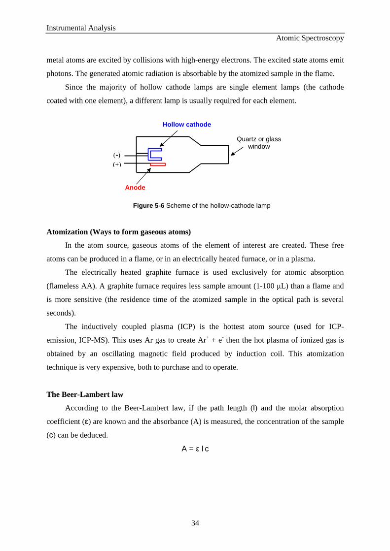
metal atoms are excited by collisions with high-energy electrons. The excited state atoms emit

photons. The generated atomic radiation is absorbable by the atomized sample in the flame.

Since the majority of hollow cathode lamps are single element lamps (the cathode

coated with one element), a different lamp is usually required for each element.

Atomization (Ways to form gaseous atoms)

In the atom source, gaseous atoms of the element of interest are created. These free

atoms can be produced in a flame, or in an electrically heated furnace, or in a plasma.

The electrically heated graphite furnace is used exclusively for atomic absorption

(flameless AA). A graphite furnace requires less sample amount (1-100 µL) than a flame and

is more sensitive (the residence time of the atomized sample in the optical path is several

seconds).

The inductively coupled plasma (ICP) is the hottest atom source (used for ICP-

emission, ICP-MS). This uses Ar gas to create Ar+ + e- then the hot plasma of ionized gas is

obtained by an oscillating magnetic field produced by induction coil. This atomization

technique is very expensive, both to purchase and to operate.

The Beer-Lambert law

According to the Beer-Lambert law, if the path length (l) and the molar absorption

coefficient (ε) are known and the absorbance (A) is measured, the concentration of the sample

(c) can be deduced.

A = ε l c

(-) (+)

Hollow cathode

Anode

Quartz or glass window

Figure 5 -6 Scheme of the hollow-cathode lamp


35

5.2 Practice

Procedure 1 – Concentration determination of potassium ion (K+) solution by atomic

emission spectroscopy (calibration curve method)

Materials: 50 ppm K+ stock solution (1 ppm = 10-6 g/cm3 = 10-6 g/mL)

Equipments: 6 pcs. volumetric flask (50.00 mL); automatic pipette

Step 1. Prepare five potassium ion solutions containing K+ in 1, 2, 3, 4 and 5 ppm

concentration from a 50 ppm K+ stock solution. Dilute the appropriate volumes of the stock

solution with distilled water in 50.00 mL volumetric flasks. (Fill 1, 2, 3, 4 and 5 mL 50 ppm

K+ stock solution into the flasks, and fill all to mark.) This will be the series of the calibration

solution.

Step 2. Measure (five times!) and record the emissions of the solutions at 766.5 nm.

Use distilled water for blank. Fill in the table.

E1 E2 E3 E4 E5 EAverage

EStandard

deviation

1 ppm 2 ppm 3 ppm 4 ppm 5 ppm Unknown

Data analysis

Step 1. Calculate the average and the standard deviation of the 5 emission data obtained

for each solution.

Step 2. Plot the averaged emission intensity versus the concentration of K+ on

millimeter squared paper. Draw a linear curve graphically on the data points.

Step 3. Use the least square method to calculate the regression line.

Step 4. Calculate the unknown potassium-ion concentration in parts per million (ppm)

according to the graphically fitted calibration curve and also from the calculated regression

equation. From y=ax+b you can get the concentration, as E unknown=ax+b, where x will be the

unknown concentration.


36

Procedure 2 – Concentration determination of copper ion (Cu2+) solution with atomic

absorption spectroscopy (Standard addition experiment)

Materials: 100 ppm Cu2+ solution; unknown Cu2+ solution

Equipments: 6 pcs. volumetric flask (25.00 mL); automatic pipette

Step 1. Prepare the following solutions in 25.00 mL volumetric flasks:

Absorbance

1. flask 0.25 mL of unknown Cu2+ solution → fill to the mark with distilled water and mix it

2. flask 0.25 mL of unknown Cu2+ solution + 0.25 mL 100 ppm Cu2+ solution → fill to the mark with distilled water and mix it





Step 2. Measure (five times!) and record the absorbance of the solutions at 324.8 nm.

The blank solution is the distilled water.

Data analysis

Step 1. Calculate the average and the standard deviation of the 5 absorbance data

obtained for each solution.

Step 2. Calculate the concentration of Cu2+ solutions in each flask, excluding the

unknown concentration of the sample solution. Prepare a table with concentration of Cu2+

solutions in the rows and 5 absorbance data; AAverage; AStandard deviation in the columns (similar

which was used in K+ concentration determination).

Step 3. Plot the averaged absorbance versus the concentration of Cu2+ on millimetre

paper. Fit a linear curve graphically on the data points.


37

Step 4. Calculate the unknown Cu2+ concentration in the solution in parts per million

(ppm) according to the graphically fitted curve. Extrapolate the regression line into the

“negative concentration” region; obtain the concentration of the unknown solution as the

intercept of the regression line with the X-axis.

5.3 Questions

1. What is the basis of the atomic emission spectroscopy/atomic absorption

spectroscopy?

2. Describe the functions of the parts of a flame atomic emission/atomic absorption

spectrometer.

3. What is the role of the monochromator?

4. How does the photomultiplier tube work?

5. How does the hollow-cathode lamp work?

6. What are the advantages of the graphite furnace comparing to the flame?

7. What is the Beer-Lambert law?

Instrumental Analysis Chromatographic Separation

38

Chapter 6 – Introduction to Chromatographic Separation

6.1 General Description of Chromatography

Chromatography is a widely used method for the separation, qualitative identification

and quantitative determination of the closely related chemical components of complex

mixtures. All chromatographic separations use a stationary phase and a mobile phase (solvent,

eluent). The samples are dissolved in a mobile phase, which may be a gas, a liquid, or a

supercritical fluid. The mobile phase is passing through the stationary phase carrying with it

the sample mixture. The stationary phase is a phase that is fixed in place in a column or on a

solid surface.

6.2 Classification of Chromatographic Methods

Chromatographic methods have two basic types. In column chromatography, the

stationary phase is held a narrow tube through which the mobile phase is forced through by

pressure. In planar chromatography, the stationary phase is supported on a flat surface or in

the pores of a paper, and the mobile phase passes through the stationary phase by capillary

action or under the influence of gravity.

A more fundamental classification of chromatographic separations is based on the types

of mobile and stationary phases and the kinds of equilibria involved in the transfer of solutes

between the phases. Table 6-1 shows three general categories of chromatography: gas

chromatography (GC), liquid chromatography (LC), and supercritical fluid

chromatography (SFC). The names imply that the mobile phases in the three techniques are

gases, liquids, and supercritical fluids. The second column of the table reveals the various

types of liquid chromatography and gas chromatography. They differ in the nature of the

stationary phase and the types of equilibra between the phases.


39

General Classification Specific Methods Stationary Phase Type of Equilibrium 1. Gas chromatography

(GC) a. Gas-liquid

(GLC) Liquid adsorbed or bonded to a solid surface

Partition between gas and liquid

b. Gas-solid Solid Adsorption 2. Liquid chromatography

(LC) a. Liquid-liquid,

or partition Liquid adsorbed or bonded to a solid surface

Partition between immiscible liquids

b. Liquid-solid, or adsorption

Solid Adsorption

c. Ion exchange Ion-exchange resin

Ion exchange

d. Size exclusion Liquid in interstices of a polymeric solid

Partition/sieving

e. Affinity Group specific liquid bonded to a solid surface

Partition between surface liquid and mobile liquid

3. Supercritical fluid chromatography (SFC), mobile phase: supercritical fluid

Organic species bonded to a solid surface

Partition between supercritical fluid and bonded surface

Chromatography is divided into categories on the basis of the mechanism of interaction

of the solute with the stationary phase:

Adsorption chromatography: a solid stationary phase and liquid or gaseous mobile

phase are used. Solute is adsorbed on the surface of the solid particles. The more strongly a

solute is adsorbed, the slower it travels through the column.

Partition chromatography: a liquid stationary phase is bonded to a solid surface, which

is typically inside the pores of porous of the silica (SiO2) chromatographic column in gas

chromatography. Solute equilibrates between the stationary liquid and the mobile phase,

which is a flowing gas in gas chromatography.

Ion-exchange chromatography: Anions such as –SO3- or cations such as –N(CH3)3

+ are

covalently attached to the stationary solid phase, usually a resin. Solute ions of the opposite

charge are attracted to the stationary phase. The mobile phase is a liquid.

Molecular exclusion chromatography: Also called size exclusion, gel filtration, or

gel permeation chromatography, this technique separates molecules by size, with no attractive

interaction between the stationary phase and solute. Rather, the liquid mobile phase passes

through a porous gel. The pores are small enough to exclude large solute molecules but not

Table 6-1 Classification of Column Chromatographic Methods


40

the small ones. Large molecules stream past the particles without entering the pores. Small

molecules take longer time to pass through the column because they enter the pore and

therefore must visit a larger volume before leaving the column.

Affinity chromatography: this most selective kind of chromatography employs

specific interactions between one kind of solute molecule and a second molecule that is

covalently attached (immobilized) to the stationary phase. For example, the immobilized

molecule might be an antibody to a particular protein. When a mixture containing a thousand

proteins is passed through the column, only the one protein that reacts with the antibody binds

to the column. After all other solutes have been washed from the column the desired protein is

dislodged by changing the pH or ionic strength.

6.3 Elution in Column Chromatography

Figure 6-1 shows how two components A and B of a sample are resolved in a packed

column by elution. Elution is a process in which solutes are washed through a stationary

phase by the movement of a mobile phase. Mobile phase, which entering the column called

eluent. Fluid which emerging from the end of the column is called eluate.

The chromatogram is a graph showing the detector response as a function of elution

time. The chromatogram is useful for both qualitative and quantitative analysis. The position

Figure 6 -1 Diagram showing the separation of a mixture of components A and B by column elution chromatography


41

of the peak maxima on the time axis can be used to identify the components of the sample.

The peak areas provide a quantitative measure of the amount of each species.

Figure 6-2 shows a simple chromatogram of a two-component mixture. The small peak

on the left is not retained by the stationary phase. The time tm after sample injection for this

peak to appear is sometimes called the dead or void time. The dead time (void time), tm, is the

time (min) it takes for an unretained species to pass through a chromatographic equipment

and column. The retention time, tr, for each component is the time (min) that elapses between

the injection of the sample onto the column and the arrival of the maximum concentration of

that component at the detector. Retention volume, Vr, is the volume (cm3) of mobile phase

required to elute a particular solute from the column.

6.4 Important Chromatographic Quantities and Relationships

The partition coefficient, K, is the ratio of concentrations of solute in the stationary and

mobile phases.

Partition coefficient: K = m

s

cc

where cs is the concentration of solute in the stationary phase, cm is the concentration of

solute in the mobile phase.

Figure 6-2 Chromatogram of a two-component mixtrue


42

The retention volume, Vr is the volume (cm3) of mobile phase required to elute a

particular solute from the column. The volume flow rate of the mobile phase is u (volume per

unit time).

Retention volume: Vr = tr u

The adjusted retention time, tr’, for a retained solute, is the additional time required to

travel the length of the column, beyond that required by solvent.

Adjusted retention time: tr’ = tr - tm

The adjusted retention volume, Vr’, is the volume (cm3) of the eluent that passed

through the column while the component was retained on the surface. These volumes are

different for every component of the sample. It takes volume Vm to push solvent from the

beginning of the column to the end of the column.

Adjusted retention volume: Vr’ = Vr - Vm

For each peak in the chromatogram, the retention factor, k, is calculated as adjusted

retention time normalized by tm.

Retention factor: k = m

mr

ttt −

= m

'r

tt

= mm

ss

Vc

Vc

where Vs is the volume of the stationary phase, Vm is the volume of the mobile phase.

For two components A and B, the relative retention (separation factor), α, is a ratio of

their adjusted retention time.

Relative retention: α= 'rA

'rB

tt

= A

B

kk

= A

B

KK

For component B eluted after component A, the unadjusted relative retention, γ, is the

ratio of their unadjusted retention times.

Unadjusted relative retention: γ = rA

rB

tt


43

In chromatography, the resolution, R, of two peaks is defined.

Resolution: R =

2BA

rArB

ww)t()t(

+−

=

2BA

rArB

ww)V()V(

+−

=

2

5890

2121 B/A/

rArB

)w()w()]t()t[(.

+−

where wA and wB are the width of A and B Gaussian peaks, and (w1/2)A and (w1/2)B are the

width at half-height of A and B Gaussian peaks.

The plate model supposes that the chromatographic column contains a large number of

separate layers, called theoretical plates. Separate equilibrations of the sample between the

stationary and mobile phases occur in these “plates”. The analyte moves down the column by

transfer of equilibrated mobile phase from one plate to the next. It is important to remember

that the plates do not really exist; they are a figment of the imagination that helps us

understand the processes at work in the column. They also serve as a way of measuring

column efficiency, either by stating the number of theoretical plates, N, in a column.

Number of theoretical plates: N=162

wt r = 5.54

2

21

/

r

wt

Plate height / Height Equivalent to a Theoretical Plate, H, is approximately the length

of column required for one equilibration of solute between mobile and stationary phases.

Figure 6-3 Resolution of some chromatographic peaks


44

Plate height: H = NL

where L is length of the column.

6.5. Keywords, abbreviations

eluent, elution, eluate, mobile phase, stationary phase, retention time, retention factor,

retention volume, relative retention, chromatogram, selectivity factor, plate height, column

resolution

6.4. Questions

1. What are the major differences between liquid-liquid and liquid-solid

chromatography?

2. What are the major differences between liquid-liquid and gas-liquid

chromatography?

3. Describe how the retention factor for a solute can be calculated?

4. Describe how the number of plates in a column can be calculated?

5. How can the selectivity factor be calculated in LC?

Instrumental Analysis Gas Chromatography

45

Chapter 7 – Gas Chromatography

Gas chromatography is a widely used analytical method, which can be used for the

analysis of thermally stable, volatile organic and inorganic compounds via a separation

procedure.

Gas chromatography (GC) can be used for example in environmental science,

brewing, food industry, perfumery and flavour analysis, petrochemical industry,

microbiological analyses, pharmaceutical industry and clinical biochemistry.

The advantages include high efficiency, selectivity, requirement for small volumes of

sample, and that the separation of the components are not destroyed during the separation

process, so with related techniques (e.g, with GC-MS) the analysis can be carried out further.

7.1 Theory

In order to get a full background to this chapter it is strongly advised first to study

Chapter 6 – Introduction to Chromatographic Separation.

Chromatography encompasses a diverse and important group of separation methods

that permit the scientist to separate, isolate, and identify closely related components of

complex mixtures; many of these separations are impossible by other means.

Chromatographic methods employ a stationary phase and a mobile phase. Components of a

mixture are carried through the stationary phase by the flow of the mobile one; separations are

based on differences in migration rates among the sample components.

Gas chromatography can be used for the separation of thermally stable, volatile

organic and inorganic compounds.

Two types of gas chromatography are encountered: gas-solid chromatography and

gas-liquid chromatography. Gas-solid chromatography employs a solid stationary phase, in

gas-liquid chromatography the stationary phase is a liquid.

In gas chromatography (Figure 7-1) the most common method of sample injection

involves the use of a microsyringe to inject a liquid or gaseous sample through a self-sealing,

silicone-rubber diaphragm or septum into a flash vaporizer port located at the head of

chromatographic column (capillary column) and separated analytes flow through a detector,

whose response is displayed on a computer. Injection of the sample may be made manually or

using an autosampler. Elution is brought about by the flow of an inert gaseous mobile phase


46

(helium, nitrogen and hydrogen). The choice of gases is often dictated by the type of detector

used. In contrast to most other types of chromatography, the mobile phase does not interact

with molecules of the analyte; its only function is to transport the analyte through the column.

When the chromatographic conditions are properly selected, the sample components

are separated on the stationary phase and they will reach the detector in the reverse order of

their interaction strength.

The chromatographic separation factors depend on the nature and velocity of the

carrier gas, the temperature, the length and internal diameter of column, the type and

thickness of stationary phase.

The detector senses the separated components, measuring some physical or chemical

properties. The detector signal can be employed for qualitative identification and quantitative

determination of separated components.

The chromatogram is a graph showing the detector response as a function of elution

time. It has two main parameters: the retention time (tR) and the peak area. Retention time is

used for the qualitative analysis of components. Quantitative analysis is based on the area of a

peak. In the linear response concentration range, the area of a peak is proportional to the

quantity of that component.

Kolonna Gáz

palack

Szűrő Áramlás és nyomás-

szabályozó

Injektor

Detektor Jelerősítő

Vezérlés

Gas Column

Filter Amplifier

Detector Injector Flow and pressure controller

Syringe

Computer

Figure 7-1 Schematic diagram of a capillary GC system


47

The Kováts retention index

The Kováts retention index (Ix) can be used for the identification of components. By

definition, the retention index for a normal alkane is equal to 100 times the number of carbon

atoms in the compound. For a homologous series, the plot of the logarithm of adjusted

retention time (tR’) versus the number of carbon atoms is linear, provided that the lowest

member of the series is excluded.

Retention index:

where n is the number of carbon atoms in the smaller alkane; n+1 is the number of carbon

atoms in the larger alkane; tR,n is the adjusted retention time of the smaller alkane; tR

,n+1 is the

adjusted retention time of the larger alkane; and tR,x is the adjusted retention time of the

unknown component (tR’n+1 > tR’x > tR’n ).

7.1.1 The main parts of GC

Gas Systems

The most common mobile phases for GC are helium, nitrogen and hydrogen, which

have the advantage of being chemically inert. The choice of gases is often dictated by the type

of detector used. The gases of flame ionization detector are hydrogen and air.

Injector

Several capillary injectors are available, the most common of which is a split / splitless

injector (Figure 7-2). Injection takes place into a heated glass or quartz liner rather than

directly onto the column.

In the split mode, the sample is split into two unequal portions the smaller of which

goes onto the column. This technique is used with concentrated samples.

In the splitless mode, the entire sample is introduced onto the column.

ntt

ttI

nn

nX

RR

RRx 100

lglg

lglg*100

''

''

1

+−−

=+


48

Column

Two general types of columns are encountered in gas chromatography, packed and

capillary. Capillary columns (Figure 7-3) are made from fused silica, usually coated on the

outside with polyimide to give the column flexibility. The wall of the column is coated with

the liquid stationary phase. The most common type of coating is based on organo silicone

polymers, which are chemically bonded to the silanol groups on the wall of the column and

the chains of the polymers are further cross-linked.

Important factors in the separation are the length and internal diameter of column, the

type and thickness of stationary phase.

The column is ordinarily housed in a thermostated oven. The optimum column

temperature depends upon the boiling point of the sample and the degree of separation

required. The ovens can be programmed to either produce a constant temperature, isothermal

conditions or a gradual increase in temperature.

Figure 7-2 A split / splitless injector

Figure 7-3 A capillary column


49

Detector

Detectors used in GC vary in nature depending upon the characteristics of the analyte

and the circumstances of its determination.

The flame ionization detector (Figure 7-4) is the most widely used and generally

applicable detector for gas chromatography. The eluent is mixed with hydrogen and then with

air. When solute molecules contained in the carrier gas elute from the column and pass into

the detector they are combusted in the flame and in doing so, generate ions which move to the

collector electrode, due to the potential difference between the jet and the electrode. The

resulting ionisation current is amplified and fed to the data system.

7.2 Practice

Conditions for Gas Chromatography

(Details of the instrument used, settings, working parameters, solvents and samples)

Gas chromatograph: Agilent Technologies 6890N GC (Figure 7-5)

Injector: split-splitless, manual and autosampler, T=270°C

Column: capillary column, Hp-1ms (25 m × 0.2 mm × 0.33 µm)

Detector: flame ionization detector (T=270°C)

Temperature program:

100°C (10 min)

100°C (0.5 min)→ 35°C /min →240°C (0 min)

Anode (+)

Air

Gasket

Hydrogen-air flame

Hydrogen

Column

Cathode (-)

Figure 7-4 A typical flame ionization detector


50

Carrier gas: helium, flow rate 1.5 mL/min

Injection volume: 1 µL

Injection mode: splitless, manual

Solvents and Samples:

n-alkanes (octane, decane and dodecane) dissolved in n-pentane

two unknown components dissolved in n-pentane

standard components dissolved in n-pentane

Manual Injection

After cleaning the syringe several times with solvent (n-pentane), take up 1 µL of

sample and 0.5 µL air then push the needle through the rubber septum into the heated

injection port of the chromatograph. Remove the syringe then start the measurement with start

button.

Capillary Column inside

Oven

Gas

Mass Selective Detector

Autoinjection System

Autosampler

Figure 7 -5 Agilent Technologies 6890N GC


51

Procedure 1 – Calculate the Kováts retention index of unknown components.

Inject the sample of n-alkanes dissolved in n-pentane and record the

chromatogram.

Inject the sample of unknown components dissolved in n-pentane and record

the chromatogram.

Calculate the Kováts retention index of unknown components.

Identify the components.

Procedure 2 – Qualitative analysis by standard components.

Inject the standard components dissolved in n-pentane and record the

chromatograms.

Procedure 3 – The examination of temperature as a factor affecting separation.

Inject the sample of known components dissolved in n-pentane, measure at a

temperature program and record the chromatogram.

Compare the chromatograms of isothermal and programmed temperature

measurements.

Procedure 4 – Characterize the separation of the components in the sample.

Calculate the k, α, R, N, H, R parameters with the help of the table and the

chromatogram recorded under the practice.

Parameter Report Component 1 Component 2 tM tR tR’ k’ w α N H R


52

Concepts and Abbreviations

Gas chromatography, GC, injector, stationary phase, mobile phase, capillary column, flame

ionisation detector, chromatogram, retention time, Kováts retention index.

7.3 Questions

What is the gas chromatography?

What are the main parts of the gas chromatograph?

What happens to be the principle of separation of components?

How does the flame ionization detector work?

What is the chromatogram?

What is the retention time?

List some factors affecting the separation and explain their effect.

Instrumental Analysis High Performance Liquid Chromatography

53

Chapter 8 - High-performance liquid chromatography (HPLC)

8.1 Introduction

In order to get a full background to this chapter it is strongly advised first to study

Chapter 6 – Introduction to Chromatographic Separation.

HPLC is an acronym, related to a separation technique; the most widely used

analytical method to separate the components of a complex mixture. The explanation of the

term HPLC is the following:

C – Chromatography: a group of separation techniques utilizing the mass-transfer between

a stationary and a mobile phase.

LC – Liquid Chromatography : one class of chromatography, the applied mobile phase is

in liquid state.

HPLC – High Performance Liquid Chromatography: high performance is the result

of many factors:

(1) very small particles of narrow distribution range,

(2) uniform pore size and pore size distribution,

(3) high pressure column slurry packing techniques,

(4) accurate low volume sample injectors,

(5) sensitive low volume detectors,

(6) high pressure pumping systems.

8.2 Types of HPLC

Based on the chemical nature of the stationary phase, and on the retention

mechanism, HPLC can be divided into three types, which cover almost 90% of all

chromatographic applications.

I. Adsorption chromatography: the stationary phase is an adsorbent, and the retention

mechanism is based on repeated adsorption and desorption steps.


54

• Normal-phase chromatography: in which the stationary phase or adsorbent is more

polar than the mobile phase or eluent. For example, the adsorbent can be silica or

alumina, and the solvent can be n-hexane or diethyl-ether.

• Reversed-phase chromatography: in which the stationary phase is nonpolar or

weakly polar and the solvent is more polar (just the opposite as in normal phase

chromatography). The stationary phases are usually chemically modified silicas,

during the modification using alkyl-chains the surface of the silica gel becomes apolar.

The mobile phases are usually polar mixtures of an organic component (methanol,

acetonitrile etc.) and water.

II . Ion-exchange chromatography: the stationary phase has a charged surface with

opposite charges on it compared to the sample ions. This technique is used almost only

for ionic or ionizable samples. The mobile phase is an aqueous buffer with controlled

pH and ionic strength.

III. Size exclusion chromatography: the stationary phase is made of a material with

precisely controlled pore size. The larger molecules rapidly pass the column, while the

smaller ones penetrate into the pores and washed out later by the mobile phase.

Figure 8-1 SEM-image of porous silica-gel particles Figure 8-2 Chemical modification of the silica using octadecyl ligands (C18)


55

8.3 The HPLC instrument

8.3.1 Flasks for the mobile phase storage

Using high- pressure pumps to deliver liquid, the solvents have to be gas-free in

HPLC experiments. The excess gas in the mobile phase causes several problems during the

analysis. Because of the compressibility of the gases, the pump pressure and the flow rate

will fluctuate, and it would cause significant disturbance in the detection and in the

repeatability of the chromatographic data. Due to those reasons, the mobile phase has to be

degassed. Degassing may be accomplished by one of the following methods or their

combination:

Degassing the liquid under vacuum – heavy-walled flask is really important, in this

case.

Heating the liquid until its boiling occurs.

Placing the container of liquid in an ultrasonic bath, or inserting an ultrasonic probe

in it.

Bubbling a fine stream of helium through the liquid; helium has the unique

ability to purge other gases out of solutions.

Some instruments are equipped with built-in degasser, but its capacity is not

enough in every case.

8.3.2 Pumps

The pumps applied in the practice of HPLC have to provide a constant and almost

pulse-free flow of the mobile phase through the system. If we use one pump, the

Figure 8-3 Typical HPLC instrument with computer data acquisition station


56

composition of the mobile phase is constant during the experiment, which is called isocratic

elution. With the aid of two or more pumps, using a time program, the composition of the

mobile phase is variable. When the mobile phase composition is changing during the

analysis, the technique is called gradient elution.

8.3.3 Injectors

Injectors for liquid chromatographic systems should provide the possibility of

injecting the liquid sample within a large volume range with high reproducibility and

under high pressure (up to 1200 bar). They should also produce minimum band broadening

and minimize possible flow disturbances. Generally, the most useful and widely used

sampling device for modern LC is the six-port Rheodyne valve.

In the six-port Rheodyne valve, the sample is introduced into the sample loop (in load

position) using a special syringe. A clockwise rotation of the valve rotor (inject position)

places the sample-filled loop into the mobile-phase stream, with subsequent injection of

the sample onto the top of the column through a low-volume, cleanly swept channel.

8.3.4 Columns

The column is the heart of the HPLC instrument, this is the part where the

stationary phase is immobilized, and the retentions of the compounds take place. Modern

HPLC column beds used in adsorption chromatography are small rigid porous particles with

high surface area.

Figure 8-4 Manual six-port injector with the two positions for sample introduction (E=eluent)


57

Nowadays, stainless steel is chosen for the material of the column housing because it

offers the best compromise of cost, workability, and corrosion resistance. Depending on the

chromatographic procedure, the column length and diameter can change in a wide range. In

modern instruments, a column thermostat is used to ensure the constant temperature in the

column during the separation.

8.3.5 Detectors

Detectors equipped with the flow-through cell were a major breakthrough in the

development of modern liquid chromatography. Such detection was first applied by the

group of Tiselius, in Sweden in 1940, by continuously measuring the refractive index of the

column effluent. Current LC detectors have wide dynamic range, and have high

sensitivities often allowing the detection of nanograms of material. A few types of

detectors:

Refractive index detector

UV/VIS detector

Fluorescence detector

Conductivity detector

Mass-spectrometric detector (MS)

In the last decade there has been a significant progress in the development of LC/MS

interfacing systems. MS as an on-line HPLC detector is said to be the most sensitive,

selective and in the same time the most universal detector. But it is still the most expensive

one.

Figure 8-5 LC columns with different lengths and diameters


58

8.4. Practice

Quantitative analysis of active substances of Saridon analgetic by RP-HPLC

Instrument

Glass flasks for the eluents

Degasser: DGU-14A VP (Shimadzu, Japan)

Pumps: LC-10AD VP (Shimadzu, Japan)

Injector: 7125 Rheodyne injector (Rheodyne, USA) with 2 µL sample loop

Diode Array Detector: SPD-M10A VP (Shimadzu, Japan)

System Controller: SCL-10A VP (Shimadzu, Japan)

PC with Labsolutions chromatographic software (Shimadzu, Japan)

Chromatographic conditions

Column: BDS Hypersil C18 (100×4.6 mm, 3µm, Thermo Scientific, USA)

Mobile phases (eluents):

o A: 0.1 v/v% trifluoroacetic acid in water

o B: 0.1 v/v% trifluoroacetic acid in methanol

Column temperature: ambient

Injection volume: 2 µL

Separation mode: for the separations different kind isocratic and gradient elution

modes will be set.

Detection wavelengths: depend on registered spectra.

Chemicals

water, methanol, thiourea, trifluoroacetic acid, paracetamol and caffeine standards, Saridon

tablet

Structural formula of paracetamol and caffeine

HO

N

H

O

N

NH3C

N

N

CH3

O

CH3

O

paracetamol caffeine


59

Step 1. Column characterization

Determine the dead or void time (tm) and the dead or void volume (Vm) of the column using

thiourea as nonretained marker.

Elution steps uv (mL/min)

tm (min)

Vm (mL)

Isocratic 1

Isocratic 2

Isocratic 3

Isocratic 4

Gradient 1

Gradient 2

Step 2. Qualitative analysis of the caffeine and paracetamol standards

Determine the retention time (tr ) of paracetamol and caffeine, by injecting standard

solutions.

Calculate the following chromatographic parameters from the chromatogram of

standard solutions for paracetamol and caffeine compounds:

o adjusted (reduced) retention time, tr’

o retention volume (Vr ),

o retention factor (k) of paracetamol and caffeine, by injecting standard

solutions. Repeat the injections at least three times.

Step 3. Effect of the experimental parameters on the retention volumes of paracetamol and

caffeine

Determine the effect of the methanol concentration under isocratic conditions on the

retention volumes of the studied compounds. Try the separation using different

gradient programs.

Table 8-1 Column characterization


60

Elution steps

uv (mL/min)

tp (min)

tp’

(min) Vp

(mL) Vp

’

(mL) wp

(min) Np Hp

(µm) k' p

Isocratic 1

Isocratic 2

Isocratic 3

Isocratic 4

Gradient 1

Gradient 2

Elution steps

uv (mL/min)

tc (min)

tc’

(min) Vc

(mL) Vc

’

(mL) wc

(min) Nc Hc

(µm) k' c

Isocratic 1

Isocratic 2

Isocratic 3

Isocratic 4

Gradient 1

Gradient 2

Elution steps R α

Isocratic 1

Isocratic 2

Isocratic 3

Isocratic 4

Gradient 1

Gradient 2

Step 4. Calibration curve

Dilute four times the standard solution, and measure the peak area of the standards

with five known concentrations. Construct a calibration curve of peak area versus

concentration. Calculate the peak areas from the average of the three injections.

Table 8-2 Effect of the experimental parameters on the retention volumes of paracetamol and caffeine


61

Step 5. Qualitative analysis

Inject the Saridon tablet solution and determine the concentration of caffeine and

paracetamol based on the measured peak areas, and the calibration curve.

Calculate the concentration of the pharmaceutically active compounds in one tablet.


theory of high-performance liquid chromatography,

detailed parts of the HPLC equipment,

detailed description of the measurements (HPLC equipment settings, eluents,

column, working parameters),

determined and calculated chromatographic parameters.


high-performance liquid chromatography, bonded stationary phase, dead volume,

derivatization, eluent strength, gradient elution, isocratic elution, guard column, porous

particle, normal-phase chromatography, reversed-phase chromatography, ultraviolet detector,

diode array detector,

LC, NP-HPLC, RP-HPLC, UV-Vis, DAD

8.6 Questions

1. What is the definition of chromatography?

2. What is liquid chromatography?

3. What is the difference between normal-phase and reversed-phase chromatography?

4. Define the retention volume, and the retention factor.

5. What is the chromatogram?

6. Define the main parts of an HPLC instrument.

7. What are the differences between isocratic and gradient elution?

8. Why is high pressure needed in HPLC?

9. How can the dead or void time be measured?

Instrumental Analysis Mass Spectrometry

62

Chapter 9 – Mass spectrometry

9.1 Theory

Mass spectrometry is a widely used technique in chemistry, biochemistry, pharmacy,

and medicine. It is also a high-performance analytical tool for structure analysis of organic

compounds. It has high sensitivity, low detection limits, high reproducibility, extremely low

sample consumption; and samples can be analyzed with different mass spectrometric

techniques even in gas, liquid or solid state. Mass spectrometry can be powerfully combined

with gas chromatography, liquid chromatography, and capillary electrophoresis.

The basic principle of mass spectrometry (MS) is to generate gas-phase ions from the

sample, to separate these ions by their mass-to-charge ratio (m/z) and to detect them

qualitatively and quantitatively by their respective m/z and abundance.

The general scheme of mass spectrometers is shown in Fig. 9-1. Basically a mass

spectrometer consists of an ion source, a mass analyzer and a detector. The mass analysis and

the detection of the ions take place under high vacuum conditions which are provided by the

vacuum system. Most of the ion sources are operated under high vacuum, although novel ion

sources have been introduced which work under atmospheric pressure. The properties of the

sample (e.g., it is in gas, liquid, or solid state, or its polarity, acidity, solubility in different

solvents, etc.) determine the sample inlet and ion source combination to be chosen for the

mass spectrometric analysis. Ion optics transfers the ions from atmospheric pressure of the ion

source to the high vacuum of mass analyzer via different vacuum stages. A data system is

used to collect and process data from the detector and, nowadays, it also controls all functions

of the instrument.

Vacuum system

Ion optics Mass analyzer Detector

Sample inlet

Data system

Ion source

Vacuum system

Ion optics Mass analyzer Detector

Sample inlet

Data system

Ion source

Figure 9-1 General scheme of a mass spectrometer


63

9.1.1 Ion sources working under atmospheric pressure

Electrospray (ESI): ionization process which uses an electrical field to generate

charged droplets and subsequent gas-phase analyte ions. In many conventional ESI sources,

nebulization of the liquid-phase sample is pneumatically assisted with the addition of a flow

of nebulizer gas (e.g. nitrogen) (see Fig. 9-2).

Briefly, the electrospray ionization comprises the following steps. Potential difference

is applied between the sample inlet capillary and the counter electrode (usually between 2-5

kV). The electric field causes electrophoretic charge separation in the solution at the capillary

tip and generates a mist of highly charged droplets. The charged droplets are attracted toward

the capillary sampling orifice through a counter flow drying gas (e.g. heated nitrogen), which

shrinks the droplets and carries away uncharged material. Thus the droplets reduce in size by

evaporation of the solvent or by ‘Coulomb explosion’ (droplet subdivision resulting from the

high charge density). Finally, fully desolvated ions result from complete evaporation of the

solvent.

Drying gas

Heated capillary

Nebulizer gas

Sample inlet

2-5 kV

Drying gas

Drying gas

Heated capillary

Nebulizer gas

Sample inlet

2-5 kV

Drying gas

Drying gas

Heated capillary

Heater

Nebulizer gas

Sample Inlet

Corona discharge

Drying gas

Drying gas

Heated capillary

Heater

Nebulizer gas

Sample Inlet

Corona discharge

Drying gas

Atmospheric Pressure Chemical Ionization (APCI): a corona discharge is used to

ionize the analytes and the species of the mobile phase or solvent in the gas phase (see Fig. 9-

3). Gas phase chemical ionization process takes place at atmospheric pressure where the

ionized solvent acts as reagent gas and ionizes the sample in gas-phase reactions.

Figure 9-2 An electrospray ion source Figure 9-3 An APCI ion source


64

Atmospheric Pressure Photoionization (APPI): ultraviolet light produced by an UV

lamp ionizes gas phase analytes or dopants added to the sample with subsequent gas-phase

reactions (see Fig. 9-4).

UV lamp

Dopant: e.g. toluene

Drying gas

Heated capillary

Drying gas

Heater

Nebulizer gas

Sample Inlet

UV lamp

Dopant: e.g. toluene

Drying gas

Heated capillary

Drying gas

Heater

Nebulizer gas

Sample Inlet

9.1.2 Quadrupole mass analyzers

Linear quadrupole (Q)

A linear quadrupole mass analyzer consists of four cylindrical metal rods set parallel

and mounted in a square configuration. The pairs of opposite rods are held at the same

potential which is composed of a direct voltage (U) and an alternating voltage component (V

amplitude with ω frequency); see Fig. 9-5. As an ion enters the quadrupole assembly, an

attractive force is exerted on it by the oppositely charged electrodes. Attraction and repulsion

are alternating in time, because the voltage applied to the rods and, thus, the sign of the

electric force also changes periodically. Only ions of a certain m/z value or m/z range pass the

quadrupole for a given set of voltages (U, V and ω). Overall, the analyzer acts as a mass filter.

The whole m/z range can be scanned with continuously varying the U, V voltages.

Figure 9-4 An APPI ion source


65

Quadrupole Ion Trap (QIT)

A quadrupole ion trap is a mass analyzer that uses an oscillating three-dimensional

quadrupole electric field to store and then eject ions. The ion trap consists of a ring electrode

between two hyperbolic endcap electrodes (see Fig. 9-6). As a high voltage RF potential is

applied to the ring electrode and the endcap electrodes are held at ground potential, an

oscillating three-dimensional quadrupole electric field is formed in the trap. This field can

keep ions of a particular m/z range within the ion trap during the ion accumulation period.

After trapping, the mass spectrum is recorded when the ions are consecutively ejected from

the analyzer by varying the three-dimensional quadrupole field.

The main advantage of an ion trap mass analyzer is the opportunity of tandem mass

spectrometric measurements in time. Tandem mass spectrometry or MS/MS, briefly, means

multiple mass analyses. After the first mass spectrometric analysis, a precursor ion is selected

Figure 9-5 A linear quadrupole mass analyzer

Figure 9-6 A quadrupole ion trap mass analyzer


66

for further analysis. It decomposes either spontaneously or as a result of additional activation

process yielding product ions or fragment ions. These ions are subjected to a second mass

spectrometric analysis, when a MS/MS spectrum is recorded.

Ion trap MS/MS is performed in one analyzer in a sequenced program of events:

1) Ion accumulation: The ion trap is loaded with ions until a maximum charge level or time

has been reached.

2) Isolation: Varying the three-dimensional quadrupole field keeps only one m/z ion, the

precursor ion, stable inside the trap.

3) Collision Induced Dissociation (CID): The precursor ion is resonantly excited to gain

energy for CID with the helium bath gas present inside the trap. The product ions are stored in

the trap. (Note step 2 and 3 can be repeated again for MS3 and so on.)

4) Scan: The product ions are mass analyzed by scanning the voltage on the ring electrode.

MSn analysis in an ion trap mass spectrometer permits multiple stages of precursor ion

isolation and fragmentation. This stepwise fragmentation permits individual fragmentation

pathways to be followed and provides extra structural information.

9.1.3 Mass spectrum

A mass spectrum is the two-dimensional representation of signal intensity or ion

abundance versus mass-to-charge ratio. The mass-to-charge ratio, m/z, is a dimensionless

quantity, because it is calculated from the dimensionless mass number, m, of a given ion, and

the number of its elementary charges, z. The most intense peak in a mass spectrum is called

base peak. In most representation the relative abundances of ions are plotted as a function of

their m/z values, i.e., the intensity of the base peak is normalized to 100 % relative intensity

and the intensities of other peaks are expressed as the percentages of the base peak intensity

(see Fig. 9-7).


67

Depending on the ionization process different ions appear in the mass spectrum. In case

of electron impact ionization mass spectrometry, the peak at highest m/z results from the

intact ionized molecule, the molecular ion (represented by M+•, e.g. C4H10+• for butane in Fig.

9-7). A molecular ion is formed by the removal of one electron from a molecule to form a

positive radical ion or the addition of one electron to form a negative radical ion. In Fig. 9-7,

the molecular ion peak at m/z 58 is accompanied by several peaks (so called fragment ion

peaks) at lower m/z caused by fragmentation or dissociation of the molecular ion. In case of

electrospray ionization mass spectrometry, different ions of the molecular species can be

detected (e.g. protonated or deprotonated molecules, adduct ions): Protonated or deprotonated

molecules, represented by [M+H]+ or [M−H]−, are ions resulting from the ionization of a

molecule by the addition or removal of a proton, respectively. A cationized molecule is an

adduct ion formed by the association of a cation with the molecule, e.g. [M+Na]+, [M+K] +.

An anionized molecule is an adduct ion formed by the association of an anion with the

molecule, e.g. [M−Cl]−.

Definitions

Average mass or chemical mass of an ion or molecule is calculated using a weighted

average of the natural isotopes for the atomic mass of each element. That is the mass

calculated from the relative atomic masses of the elements.

Figure 9-7 Electron impact ionization mass spectrum of butane


68

Nominal mass of an ion or molecule is calculated using the mass of the predominant

isotope of each element rounded to the nearest integer value and multiplied by the number of

atoms of each element.

Monoisotopic mass is the exact mass of an ion or molecule calculated using the exact

mass of the predominant isotope of each element.

Resolution: In a mass spectrum, the observed m/z value divided by the smallest

difference ∆(m/z) for two ions that can be separated: (m/z)/∆(m/z).

9.2 Practice

Structural analysis of capsaicin and dihydrocapsaicin by electrospray – ion trap MS and

MS/MS methods

Instrument:

Agilent 6300 LC/MSD Trap XCT Plus mass spectrometer equipped with

electrospray ion source and ion trap mass analyzer.

The sample solutions will be introduced into the ion source by direct infusion with a

syringe and a syringe pump.

Default MS parameters:

Drying gas (N2) flow rate: 4 L/min

Drying gas (N2) temperature: 325°C

Nebulizer gas (N2) pressure: 15 psi

High voltage: –3000 V or +3000 V

Mass-to-charge (m/z) range detected: 50-2200 m/z

Analysis speed (Ultra Scan mode): 26000 m/z/s

Other parameters of the ionization and mass analysis will be optimized during the

practice


69

Chemicals:

water, methanol, capsaicin, dihydrocapsaicin

Structural formula of capsaicin and dihydrocapsaicin:

Step 1.

Calculate the elemental formula of capsaicin and dihydrocapsaicin. Calculate the

nominal, monoisotopic and average masses of both compounds.

Atomic Symbol

Atomic Number

Mass Number

Isotopic Abundance

Isotopic Mass

Relative Atomic Mass

H 1 1 99.985 1.007825 1.00795 2 0.015 2.014101

C 6 12 98.90 12.000000 12.0108 13 1.10 13.003355

N 7 14 99.63 14.003070 14.00675 15 0.37 15.000109

O 8 16 99.76 15.994915 15.9994 17 0.04 16.999132 18 0.20 17.999116

Step 2.

Dilute the 1mg/mL stock solutions to 10 µg/mL concentration with methanol and

water. The solvent of the diluted solutions should be water−methanol 1:1 v/v.

Step 3.

Record the mass spectra of the samples in positive and negative ion modes.

Analyze the mass spectra. Based on the m/z of the ions describe ions observed in the

mass spectra.

OHN

HO

OO

HN

HO

O

capsaicin dihydrocapsaicin


70

Step 4.

Isolate the [M+H]+ and [M–H]– quasimolecular ions as precursor ions and fragment

them. Thus, record the MS/MS mass spectra for both compounds in positive and

negative ion modes.

Analyze the fragmentation mass spectra, suggest fragmentation sites of the precursor

ions and suggest empirical formula for the major fragment ions.


theory of mass spectrometry, parts of the mass spectrometer, details on electrospray

ionization, quadrupole mass analyzers, tandem mass spectrometry

detailed description of the measurements (settings, working parameters)

the elemental formula, and the calculated nominal, monoisotopic and average masses

of capsaicin and dihydrocapsaicin

(+)ESI-MS and (–)ESI-MS mass spectra with explanations of the ions

(+)ESI-MS/MS and (–)ESI-MS/MS mass spectra of the [M+H]+ and [M–H]– ions,

respectively

fragmentation sites indicated in the structural formula of the molecules

elemental formula suggested for the major fragment ions


mass spectrometer, ion source, mass analyzer, electrospray ionization, atmospheric pressure

chemical ionization, atmospheric pressure photoionization, linear quadrupole mass analyzer,

quadrupole ion trap mass analyzer, mass spectrum, mass-to-charge ratio, base peak, molecular

ion, ions of molecular species (protonated or deprotonated molecules and adduct ions),

tandem mass spectrometry, precursor ion, product ion or fragment ion, average mass or

chemical mass, nominal mass, monoisotopic mass, resolution

ESI, APCI, APPI, Q, QIT, MS/MS, MSn


71

9.4. Questions

1. What are the basic principles of mass spectrometry?

2. What are the main parts of a mass spectrometer?

3. What is a mass spectrum?

4. What are the tasks of ion sources? Name three ion sources.

5. What are the tasks of mass analyzers? Name two mass analyzers.

6. How does an electrospray ion source work?

7. Define tandem mass spectrometry.

8. Calculate the isotopic distribution of: (a) Br2, (b) Cl2.

9. Calculate the minimum resolution that is required from a mass analyzer to separate the

following isobaric species (i.e. species of the same nominal mass).

(a) CO (M=27.99491) and N2 (M=28.00615)

(b) 13CC6H7 (M=92.05813) and C7H8 (M=92.06260)

10. A protein (cytochrome C) electrospray – ion trap MS mass spectra is depicted on Fig. 8-

8. In the ESI-MS mass spectrum of a protein, normally a characteristic series of

multiply charged peaks present. In the positive ionization mode, the (M+zH)z+ ions are

formed in a multistep, consecutive protonation process. Thus each peak in the

following spectrum belongs to the same protein; the differences between the ions are

in their protonation and charge states.

(a) Calculate the molecular mass of the protein.

(b) Determine the charge number (z) of the ion corresponding to the base peak.

I [x10 6]

589.81 619.26

651.60

687.77

728.18

773.56

825.01

883.78

500 550 600 650 700 750 800 850 900 950 m/z 0.00

0.25

0.50

0.75

1.00

1.25

1.50

Figure 8-8 Electrospray mass spectrum of cytochrome C recorded in positive ion mode

Instrumental Analysis Capillary Electrophoresis

72

Chapter 10 – Capillary Electrophoresis

10.1 Theory

10.1.1 Introduction

Electrophoresis is the migration of electrically charged solute molecules (ions) in an

electric field. It can be performed in slab-gel format or in microfluidic capillary formats. In

capillary electrophoresis (CE), the electrophoretic separation of solutes is carried out in

narrow-bore tubes, typically 25 to 200 µm inner diameter (id), which are usually filled only

with buffer (electrolyte). Because of the high resistance of the electrolyte in the narrow-bore

capillary, very high electrical fields (100 to 500 V/cm) can be applied, which results in short

analysis times. The heat developed during electrophoresis is efficiently dissipated due to the

large surface area-to-volume ratio of the capillary.

Today, CE is a premier separation technique for the study of low molecular weight

substances (e.g., inorganic and organic ions, amino acids, purine and pyrimidine bases,

nucleosides, nucleotides, chiral drugs, vitamins etc.) as well as large structures (such as

proteins, nucleic acids, carbohydrates, oligonucleotides, DNA restriction fragments, virus

particles and even whole cells). Main advantages of CE include the extremely high separation

efficiency and resolution, minimal consumption of samples and buffers, on-capillary

detection, high speed of analysis, and the potential for quantitative analysis and automation.

In addition, the numerous operation modes offer different separation mechanisms and

selectivities (see table 10-1).

Mode Basis of separation

Capillary zone electrophoresis (CZE) Free solution mobility

Capillary isotachophoresis (CITP) Moving boundaries

Capillary isoelectric focusing (CIEF) Isoelectric point

Capillary gel electrophoresis (CGE) Size (mass)

Micellar electrokinetic chromatography (MEKC)

Hydrophobic / ionic interactions with micelle

Capillary electrochromatography (CEC) Chromatographic interactions

Table 10-1 Modes of capillary electrophoresis


73

10.1.2 Instrumentation

The commercial instrumentation of capillary electrophoresis is illustrated in Figure 10-

1. Typical CE systems use fused silica capillaries externally coated with polyimide, like those

applied in gas chromatography. The capillary is placed in buffer reservoirs and filled with

buffer from one of the buffer vials by applying external pressure. The sample (1-10 nL) is

introduced from the sample vial, by replacing one of the vials with the sample vial and

applying either low pressure (hydrodynamic injection) or low voltage (electrokinetic

injection). After replacing the buffer vial, the electric field is applied across the capillary by a

high voltage (HV) power supply (typically 10 to 30 kV), which connects the two electrodes

immersed in the buffer vials. The resulting electrophoretic current is usually 5 to 50 µA. The

analytes start to migrate in the capillary towards the detector and they separate by reason of

their electrophoretic mobility depending on their size and charge. Optical detection can be

made directly through the capillary. UV-Visible absorption is the most widely used detection

method. An optical window in the capillary is easily created by removal of a small (1-3 mm)

section of the protective polyimide coating. Other detectors are LIF (laser induced

fluorescence), conductivity detector, mass spectrometer, etc.

Modern CE devices also include an autosampler ideal for automation of measurement

series, and a temperature regulating unit (thermostat) ensuring constant temperature during

the separation process (observe that viscosity of the electrolytes depend on temperature).

Figure 10-1 Schematic of CE instrumentation


74

10.1.3 Background

Separation by electrophoresis is based on differences in solute velocity in an electric

field. The linear velocity of a migrating ion in an electrolyte solution is given by

v = µ E (1)

where v = ion velocity [cm/s]

µ = electrophoretic mobility [cm2/V⋅s]

E = applied electric field [V/cm]

Consequently, an increase in field strength increases the velocity. When an ion has been

accelerated to constant velocity in a constant electric field, the electric force (FE = q E) on the

ion is equal to the frictional force (FF = - 6 π η r v), which gives the relation:

qE = 6πηrv (2)

where q = ion charge

η = viscosity of electrolyte

r = solvated radius of ion

v = ion velocity

Solving for velocity and substituting equation (2) into equation (1) yields an equation

that describes the mobility in terms of physical parameters

r6q

e πη=µ

From this equation it is evident that small, highly charged ions have high mobilities

whereas large, minimally charged ions have low mobilities.

10.1.4 Electro-osmotic flow (EOF)

EOF is the bulk flow of liquid in the capillary at a constant speed induced by the electric

field. It results from the charge excess near the interior capillary wall. The inner surface of the

fused silica capillaries are covered by silanol groups (≡Si–OH), which start to dissociate to

negatively charged (≡Si–O-) groups in contact with solutions above pH 2.5. The immobilized

surface ions attract the mobile ions of opposite charge in the buffer solution (electrolyte) by


75

electrostatic forces, which arrange themselves into two layers called electrical double layer

(Figure 10-2). The net surface charge density and the thickness of the double layer are

affected by the pH and the ionic strength of the electrolyte, respectively.

The applied electric field forces the charge excess in the diffuse double layer to move

toward the cathode. The motion of these ions will draw the bulk liquid along with them,

creating a flat (plug-like) solvent flow termed electro-osmotic flow (EOF) (Figure 10-3). The

flat profile does not contribute (except in a thin layer close to the tube wall) to a broadening of

an analyte zone, as does a parabolic profile of hydrodynamic flow generated by pumps in an

open capillary, i.e., EOF only displaces the analytes. Peak efficiency in CE, often in excess of

105 theoretical plates.

The mobility of EOF is given by the Smoluchowski equation:

πηζεε

=µ4

0EOF

where µEOF = electro-osmotic mobility

ζ = zeta potential

ε = relative permittivity (dielectric constant of electrolyte)

εo = relative permittivity of the vacuum

η = viscosity of electrolyte

Figure 10-3 Plug-like flow profile of EOF

Figure 10-2 Representation of the double layer at the capillary wall


76

The zeta potential is the potential difference created close to the wall (Figure 10-4),

and is strongly dependent on the ionic strength and pH of the buffer.

10.1.5 Capillary zone electrophoresis

CZE is the simplest form of CE, because the capillary is only filled with buffer.

Separation occurs because analytes migrate in discrete zones and at different velocities, based

on their charge to size ratio. Separation of both anionic and cationic solutes is possible due to

the superposition of electro-osmotic flow on to analyte mobility (Figure 10-5).

As depicted in Figure 10-5, EOF causes movement of all species, regardless of charge,

in the same direction (from the anode to the cathode). The ions migrate with a resultant

migration velocity owing to their own electrophoretic mobility and the mobility of the EOF,

whereas neutral analytes are transported by the EOF. Cations migrate fastest as the

electrophoretic attraction towards the cathode and the EOF are in the same direction. Neutral

Figure 10-4 The electrostatic potential in the double layer

Figure 10-5 Migration order of ions in capillary zone electrophoresis in the presence of EOF


77

molecules are not separated from each other, and anions migrate slowest as they are attracted

to the anode but are still carried by the EOF toward the cathode (the magnitude of EOF can be

more than an order of magnitude greater than the electrophoretic mobilities of the analytes).

If the capillary wall is pre-treated (coated) with a neutral surfactant (either a viscous

polymer or a covalently attached polymer), the walls will be uncharged and the EOF will be

eliminated. In these circumstances, anions and cations can migrate in opposite directions.

When analyzing proteins, stable neutral coatings are needed to reduce effectively protein

adsorption onto the capillary wall.

10.1.6 Electropherogram

The result of an electrophoretic run is an electropherogram, where migration time is

plotted on the X axis and absorbance data are plotted on the Y axis (Figure 10-6). Qualitative

information of compounds is provided by the position of peaks (migration time), while

quantitative information (concentration of compounds) can be obtained from the peak height

or peak area.

10.1.7 Analytical parameters

Electrophoretic mobility

The mobility is characteristic constant for an ion in a given electrolyte, and it can be

determined from an electrophoresis experiment. Upon replacing v with l/t and E with U/L in

equation (1), the mobilities of the analytes can be determined by the following formula:

Figure 10-6 Electropherogram of benzyl derivatives


78

UtLl

a ⋅⋅=µ

where µa = apparent mobility

U = applied voltage

l = effective capillary length (from injection end to the detector)

L = total capillary length

t = migration time

In the presence of electro-osmotic flow, the measured mobility is called the apparent

mobility, µa = µe + µEOF. The effective mobility, µe, can be extracted from µa by

independently measuring the EOF using a neutral marker (e.g. acetone) that moves at a

velocity equal to the EOF.

Efficiency

In separation science, two related concepts for measuring the efficiency of separation

are widely used, the plate height (H) and the plate number (N). The theoretical plate number

for a Gaussian peak can be determined directly from an electropherogram, using the following

formula:

2

21

545

ω=

/

t.N

or

2

16

ω= t

N

where t = migration time

ω1/2 = temporal peak width at half peak height

ω = temporal peak width at the baseline

Theoretical plate number can be related to the HETP (height equivalent to a theoretical plate),

H, by

Nl

H =

where l = effective capillary length


79

Low values of H are favorable and are in the µm range for high-efficiency separation.

Resolution (R)

The resolution is a quantitative measure of the degree of separation of two sample

components and is defined as:

21

t2R

ω+ω∆=

where ∆t = difference between the migration times of the analytes

ω1 and ω2 = widths of the peaks at the baseline

10.2 Practice

Measuring of preservatives and vitamin C in lime juice

Running conditions:

Instrument:

Buffer:

Capillary length (total and effective):

Injection mode:

Temperature:

Voltage:

Polarity:

Detection wavelength:


80

Samples:

Benzoic acid, sorbic acid and ascorbic acid (vitamin C) of known concentration

(standard solutions). Lime juice.

CH3 OH

O

O

OH

O

OHOH

O

OH

OH

Sorbic acid (E200) Benzoic acid (E210) Vitamin C (E300)

MW = 112.12 g/mol MW = 122.12 g/mol MW = 174.14 g/mol

λmax = 255 nm λmax = 225 nm λmax = 265 nm

Tasks

1. Make the electrophoretic run of a mixture of standards.

2. Identify the peaks (compounds) according to their charge/mass ratio.

3. Determine t (migration time) and ω1/2 (peak width at half height) of the peaks.

4. Calculate µa (apparent mobility) of each compound.

5. Determine separation efficiency by the calculation of parameters N, H and R.

6. Make the electrophoretic run of lime juice.

7. Identify the peaks (qualitative analysis) and calculate the concentration of compounds

(quantitative analysis) by comparing the electropherogram to that of standard

mixture.


theory of the analytical method

parts of the CE

settings, working parameters

detailed description of the measurement

electropherograms

calculations

results


81

10.3 Questions

1. What is the principle of separation in capillary zone electrophoresis?

2. Define ion velocity and electrophoretic mobility.

3. What is electro-osmotic flow (EOF)? Describe its benefits and flow-profile.

4. What will be the order of migration of components in an uncoated capillary at pH 9?

5. What are the main parts of a CE instrument?

6. Name two injection modes in CE.

7. What kind of detectors can be applied in CE?

8. What is an electropherogram?

Instrumental Analysis Calculations

82

Chapter 11 – Calculations

1. Calculate the molarity of a potassium dichromate solution prepared by placing 10.3000 g

of K2Cr2O7 in a 50.00 mL volumetric flask, dissolving, and diluting to the calibration

mark.

2. Calculate the molar concentration of NaCl, to the correct number of significant figures,

if 2.1915 g of NaCl is placed in a beaker and dissolved in 50.00 mL of water measured

with a graduated cylinder. This solution is quantitatively transferred to a 300.00 mL

volumetric flask and diluted to volume. Calculate the concentration of this second solution

to the correct number of significant figures.

3. 50.00 mL of 0.200 mol/L NaOH solution is neutralized with 20.00 mL of sulfuric acid.

Determine the concentration of the acid in mol/L .

4. 20.00 mL HCl solution was titrated with 0.175 mol/L (f = 0.995) KOH solution. 17.23 mL

basic solution was added to reach the equivalence point. What was the concentration of

the sample in mol/L and mg/100 mL?

5. A sample of liquid containing phosphoric acid, it was completely neutralised by 21.60 mL

of 0.500 mol/L sodium hydroxide solution.

What mass (in milligrams) of phosphoric acid was in the sample?

OH3PONaNaOH3POH 24343 +⇔+

6. 60.00 mL of an acidified dichromate(VI) solution with a concentration 0.050 mol/L was

titrated against a 0.600 mol/L Fe2+ solution. What volume of Fe2+ solution would be

required to reach the end point of this titration?

OH7Cr2e6H14OCr 232

72 +⇔++ +−+−

7. A 0.1784 g sample of a monoprotic acid neutralizes 16.40 mL of 0.085 mol/L KOH

solution. Calculate the molar mass of the acid.

−++ +⇔ eFeFe 32


83

8. 0.3000 g of aspirin (an acid) was titrated with sodium hydroxide solution of concentration

0.100 mol/L. If the aspirin required 16.45 mL of the NaOH solution to neutralise it,

calculate the percent purity of the aspirin .

9. 150.00 mL of an aqueous sodium chloride solution contains 0.0045g NaCl.

Calculate the concentration of NaCl in parts per million (ppm).

(1 ppm =1µg/g or 1 µg/mL)

10. Using the systematic approach, calculate the pH of the following solutions

1. 0.050 mol/L HClO4;

2. 10–7 mol/L HCl;

3. 0.025 mol/L HI.

11. Consider the titration of 20.00 mL of 0.050 mol/L strong acid with 0.100 mol/L strong

base. Find the pH at the following volumes of base added and make a titration graph of

pH versus Vb.

Vb = 0.00, 1.00, 3.00, 5.00, 9.00, 9.50, 10.00, 10.50, 11.00, 12.00 and 15.00 mL.

12. What is the pH at the equivalence point when 0.100 mol/L acetic acid (pKs = 4.76) was

titrated with 0.050 mol/L NaOH solution?

13. What will be pH of the original and the final solutions as you mix 13.00 mL 0.200 mol/L

(f = 0.980) HCl solution and 20.00 mL 0.160 M (f = 0.948) KOH solution?

14. How the originally 12.50 pH of the 100.00 mL NaOH solution change after every

addition, as we add 5 times 2.00 – 2.00 mL of 0.100 mol/L HCl solution?

15. Calculate the potential of a copper electrode immersed in:

a. 0.035 mol/L Cu(NO3)2

b. 0.055 mol/L in NaCl and saturated with CuCl

c. 0.025 mol/L NaOH and saturated with Cu(OH)2.


84

16. Calculate the potential of a platinum electrode immersed in a solution that is

a. 0.0508 mol/L in K4Fe(CN)6 and 0.00548 mol/L K3Fe(CN)6;

b. 0.0360 mol/L in FeSO4 and 0.00725 mol/L Fe2(SO4)3;

c. Prepared by mixing 50.00 mL 0.075 mol/L Ce(SO4)2 with an equal volume of

0.125 mol/L FeCl2 (assume solutions were 1.000 mol/L in H2SO4 and use

formal potentials).

17. Calculate the theoretical cell potential of the following cells. If the cell is short-circuited,

indicate the direction of the spontaneous cell reaction.

a. Zn Zn2+ (0.200 mol/L) Co2+ (5.04·10-4 mol/L) Co

b. Pt Fe3+ (0.250 mol/L, Fe2+ (0.085 mol/L) Hg2+ (0.0412 mol/L) Hg.

18. Calculate the energy in joules of one photon of radiation with a wavelength of 15.00 µm.

19. Calculate the wavelength and the energy in joules associated with a signal at 280 MHz.

20. Prepare the solutions by diluting 4×10-2 w/w % FeSO4 solution. Take 2.50 mL of the

stock solution, and dilute to 15.00 mL with water. Then take 5.00 mL to the next and

dilute to 15.00 mL. Follow this 2nd sequence 3 times. What will be the concentration (in

% ) of the last (5th) solution?


85

21. You should make a calibration with standard addition. Calculate the standard

concentrations in each flasks in mol/1000 mL units.

You have a 0.150 mol/L standard ZnCl2 solution. The solutions were prepared according

this table:

22. A 6.25·10-5 mol/L solution of potassium permanganate has a transmittance of 37.5% when

measured in a 1.8 cm cell at a wavelength of 525 nm. Calculate the absorbance of this

solution and the molar absorptivity of KMnO4.

23. The logarithm of the molar absorptivity of phenol in aqueous solution is 3.812 at 211 nm.

Calculate the range of phenol concentration that can be used if the absorbance is to be

greater than 0.100 and less than 1.000 with 0.75 cm cell.

24. A typical simple infrared spectrophotometer covers a wavelength range from 5 µm to 35

µm. Express its range in wavenumbers and in hertz (Hz).

25. Consider a chromatography column in which Vs = Vm/3. Find the retention factor if K =

3 and K = 30.

26. The retention volume of a solute is 57.30 mL for a column with Vm = 15.70 mL and Vs =

11.40 mL. Calculate the retention factor and the partition coefficient for this solute.

Flask No.

mol/L

1. 10.00 mL unknown solution → fill to 100.00 mL with dist. Water

2. 10.00 mL unknown solution+ 4.00 mL standard solution → fill to 100.00 mL with dist. Water






86

27. Retention times in a gas chromatogram are 1.15 min for CH4, 7.35 min for pentane, 7.57

min for unknown, and 8.02 min for hexane. Find the Kováts retention index for the

unknown component.

28. The packed column in gas chromatography had an inside diameter 4.6 mm. The

measurement volumetric flow rate at the column outlet was 35.0 mL/min. If the column

porosity was 0.38, what was the linear flow velocity in cm/s?

29. Substances A and B have retention time of 16.25 min and 18.20 min, respectively, on a

25.0 cm column. An unretained species passes though the column in 1.35 min.

The peak widths (at base) for A and B are 1.21 and 1.33 min, respectively.

Calculate

a. The column resolution;

b. The average number of plates in the column;

c. The plate height.

30. A protein required 5.3 min to travel 80.0 cm to the detector in a 95.0 cm long capillary

tube with 31.2 kV between the ends. Find the apparent electrophoretic mobility.


87

Answers to problems

1. c = 0.700 mol/L;

2. c = 0.125 mol/L;

3. c = 0.250 mol/L;

4. c = 0.150 mol/L, m = 547.5 mg in 100.00 mL;

5. m = 0.3528 g;

6. V = 30.00 mL;

7. M = 127,9 g/mol, HI;

8. m = 296.1 mg, 98.7%;

9. 30 ppm;

10.

a. pH = 1.3;

b. pH = 7;

c. pH = 1.6;

11. pH = 1.30; pH = 1.37; pH = 1.52; pH = 1.70; pH = 2.46; pH = 2.77; pH = 7.00;

pH = 11.21; pH = 11.51; pH = 11.79; pH = 12.16

12. pH = 8.78;

13. pH = 12.17;

14. pH = 12.46; pH = 12.42; pH = 12.38; pH = 12.34; pH = 12.29;

15.

a. E = 0.294 V;

b. E = 0.199 V;

c. E = - 0.138 V;

16.

a. E = 0.303 V;

b. E = 0.723 V;

c. E = 0.690 V;

17.

a. E = - 0.409 V;

b. E = 0.0145 V;

18. E = 1.326·10-20 J;

19. E = 1.856·10-25 J; λ = 1.071 m;


88

20. c1 = 6.67·10-3 %; c2 = 2.22·10-3 %; c3 = 7.41·10-4 %; c4 = 2.47·10-4 %; c5 = 8.23·10-5 %;

21. c1 = 6.0·10-3; c2 = 1.2·10-2; c3 = 1.8·10-2; c4 = 2.4·10-2; c5 = 3.0·10-2;

22. A = 0.426, ε = 37.864 L/mol·cm;

23. c1 = 2.056·10-5 mol/L, c2 = 2.056·10-4 mol/L;

24. υ1 = 6·1013 s-1, υ2 = 8.57·1012 s-1;

25. k1 = 1.0, k2 = 10.0;

26. k = 2.65, K = 3.65;

27. I = 534;

28. uo = 9.237 cm/s

29. R = 1.535, NA = 2886, NB = 2996, N = 2941, H = 0.085 mm;

30. µo = 7.6·10-8 m2/·Vs;


89

Chemical elements listed by atomic mass

Name Symbol Atomic Mass

Hydrogen H 1.0079 Carbon C 12.0107 Nitrogen N 14.0067 Oxygen O 15.9994 Sodium Na 22.9897 Magnesium Mg 24.3050 Phosphorus P 30.9738 Sulfur S 32.0650 Chlorine Cl 35.4530 Potassium K 39.0983 Chromium Cr 51.9961 Manganese Mn 54.9380 Iron Fe 55.8450 Nickel Ni 58.6934 Cobalt Co 58.9332 Copper Cu 63.5460 Zinc Zn 65.3900 Tin Sn 118.7100 Iodine I 126.9045 Mercury Hg 200.5900 Lead Pb 207.2000

Standard Electrode Potentials

Half reaction Ered (V) Ce4+(aq) + e– → Ce3+(aq) in 1.000 M H2SO4 +0,680 Hg2+(aq) + 2e– → Hg(l) +0.854 Fe3+(aq) + e– → Fe2+(aq) +0.771 Cu+(aq) + e– → Cu(s) +0.521 Fe(CN)6

3–(aq) + e– → Fe(CN)64–(aq) +0.360

Cu2+(aq) + 2e– → Cu(s) +0.337 Co2+(aq) + 2e– → Co(s) –0.277 Zn2+(aq) + 2e– → Zn(s) –0.763


90

Bibliography

Daniel C. Harris – Quantitative Chemical Analysis

F. James Holler, Douglas A. Skoog and Stanley R. Crouch – Principles of


D. A. Skoog, D. M. West, F. J. Holler and S. R. Crouch – Fundamentals of

Analytical Chemistry

David Harvey – Modern Analytical Chemistry

David G. Watson – Pharmaceutical Analysis

Jürgen H. Gross – Mass Spectrometry – A Textbook

E. de Hoffmann and V. Stroobant – Mass Spectrometry Principle and Applications

David Heiger – High performance capillary electrophoresis

DOI: 10.15170/TTK.2014.00001

lab practice 2014-javitas - pécsi...

Documents