1

Orbit of Mercury Lab: Understanding planetary orbits and plotting the orbit of Mercury Author: Sean S. Lindsay Version 1.2 created October 2018 History: Version 1.1 created October 2017 Learning Goals

In this activity, the student will learn about planetary orbits. This includes understanding the connection between the planets position in the sky (versus the Sun in this case), and that planet’s orbital motion around the Sun.

• The elliptical shape of planetary orbits and application of Kelpler’s Laws • Characteristics related to planetary orbits: semi-major and semi-minor axes;

eccentricity; perihelion; aphelion; elongation; conjunction. • Orbital versus Synodic Period • How to determine inferior planet orbits • Error in measurements

Materials

• Protractor, straight edge, pencil, and a calculator

1. Background 1.1 Historical Perspective Since the time humans began recording their observations of the sky, it has been known that there are celestial objects that are different from the stars. The Sun, the Moon, and five other objects, which are now known as the naked-eye viewable planets Mercury, Venus, Mars, Jupiter, and Saturn did not move as the stars did. Uranus and Neptune, the other planets, are too faint to see with the unaided eye. While the daily and yearly motions of the stars behave in a relatively simple way, each star moving slightly westward by about one degree per day and remaining in a fixed pattern, the ancients identified five night-sky objects that did not follow this simple rule. These five objects displayed peculiar motions and appeared to “wander” with respect to the fixed pattern of stars earning them the name planhthV (planétés), or planets, meaning wanderer.

The planetary “wandering” behavior is characterized by: (1) most commonly moving slightly eastward relative to fixed pattern of stars night after night (prograde motion); (2) sometimes reversing their normal prograde motion and looping back in the opposite, westward, direction (retrograde motion) for a short period; (3) always appearing near to the ecliptic, the path the Sun traverses through the stars over the course of a year; and (4) moving at variable speeds. As you might imagine, creating a predictive model of our solar system that accurately accounts for these complex motions proved to be extraordinarily challenging. So much so, that understanding the orbital motion of the planets challenged astronomers for nearly 1,500 years. To describe the planetary motions, the world needed to wait for Nicolaus

2

Copernicus (1473 – 1543 CE) to begin to convince the world that the Earth was not the center of the Universe, and that the planets (including Earth) orbited the Sun.

The acceptance of Copernicus’s Sun-centered (or heliocentric) model was the cornerstone toward not only having a simple, elegant model for the structure of the solar system, but also the seed to our modern understanding of planetary orbits. While ingenious, the Copernican Model of the solar system was still plagued by lingering Aristotelean dogma that insisted that planetary orbits must be perfectly circular. It was not until the mid-17th century, with the contribution of many clever minds and the invention of the modern scientific method, that a more complete view of the structure of the solar system emerged. In the then emerging view that is now generally accepted, the orbits of the planets are not circular with the Sun at the center, but rather elliptical in shape with the Sun located at one of the two foci of the ellipse.

The first person to conceive of, and demonstrate mathematically, that orbits are elliptical in shape (See Fig. 1) was Johannes Kepler (1571 – 1630 CE). Using the data set of Tycho Brahe (1546 – 1601 CE) containing the largest number of and most accurate observations of planetary positions, Kepler formulated his three laws of planetary motion. Kepler’s Three Laws of Planetary Motion can be summarized as:

I. Elliptical Orbits (Kepler’s First Law of Planetary Motion): Planetary orbits are elliptical in shape with the Sun located at one of the foci of the ellipse.

II. Equal Time; Equal Areas: A line connecting the Sun to a planet will sweep out an equal area of the ellipse for equal time intervals.

III. Distance-Period Relation: The square of the orbital period, P, of a planet (measured in years) equals the semi-major axis, a, distance (measured in AU) cubed, or P2 = a3

These three laws of planetary motion gave an accurate mathematical description and predictive formulation to the planetary positions that could fully account for the “wandering” motion of the planets. However, they simply give mathematical legs that fit observational data, a so-called empirical solution; they do not provide the explanative how, i.e., the physics, of what governs the motions of the planets. The physical explanation for how the planets orbit the Sun in elliptical paths, such that sweep out equal areas in equal times and follow a period-squared equal semi-major axis-cubed relation requires an understanding provided by Isaac Newton (1643 – 1727 CE) of generalized laws of motion and a classical conception of gravity. Newton’s Laws of Motion and Newtonian Gravity are beyond the scope of this laboratory exercise. For additional information on Newtonian physics, see your course notes, textbook, or the immense resources of the internet.

1.2 The Elliptical Shape of Orbits To us in the modern era, it is remarkable how radical Kepler’s notion of ellipse-shaped orbits was. Any imperfect, i.e., non-circular, orbit was inconceivable. It took an enormous bending of ingrained philosophical thought for Kepler to let go of the notion of circular orbits, but in the light of Brahe’s data, it became apparent that Aristotelean ideals must be broken. However, Kepler did not immediately leap to the ellipse as the shape of orbits. Still adherent to the notion perfect forms and shapes, Kepler first tried a model for the solar system that was series of nested Platonic solids. When fine tuning of this model failed to fit Brahe’s data, Kepler finally made the leap away from ideal shapes, and tested the data against

3

orbits of “imperfect” circular shape: ellipses. The mental leap paid off, and relatively rapidly Kepler could make mathematical sense of Brahe’s data.

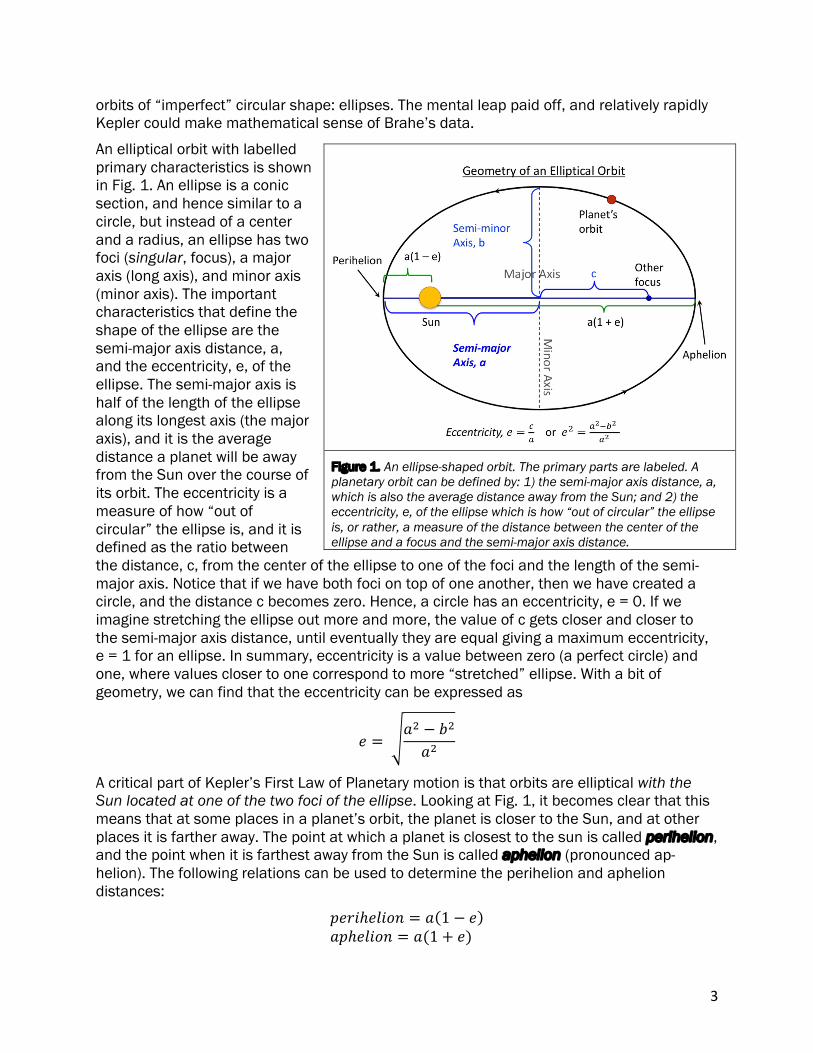
An elliptical orbit with labelled primary characteristics is shown in Fig. 1. An ellipse is a conic section, and hence similar to a circle, but instead of a center and a radius, an ellipse has two foci (singular, focus), a major axis (long axis), and minor axis (minor axis). The important characteristics that define the shape of the ellipse are the semi-major axis distance, a, and the eccentricity, e, of the ellipse. The semi-major axis is half of the length of the ellipse along its longest axis (the major axis), and it is the average distance a planet will be away from the Sun over the course of its orbit. The eccentricity is a measure of how “out of circular” the ellipse is, and it is defined as the ratio between the distance, c, from the center of the ellipse to one of the foci and the length of the semi-major axis. Notice that if we have both foci on top of one another, then we have created a circle, and the distance c becomes zero. Hence, a circle has an eccentricity, e = 0. If we imagine stretching the ellipse out more and more, the value of c gets closer and closer to the semi-major axis distance, until eventually they are equal giving a maximum eccentricity, e = 1 for an ellipse. In summary, eccentricity is a value between zero (a perfect circle) and one, where values closer to one correspond to more “stretched” ellipse. With a bit of geometry, we can find that the eccentricity can be expressed as

𝑒 = $𝑎& − 𝑏&

𝑎&

A critical part of Kepler’s First Law of Planetary motion is that orbits are elliptical with the Sun located at one of the two foci of the ellipse. Looking at Fig. 1, it becomes clear that this means that at some places in a planet’s orbit, the planet is closer to the Sun, and at other places it is farther away. The point at which a planet is closest to the sun is called perihelion, and the point when it is farthest away from the Sun is called aphelion (pronounced ap-helion). The following relations can be used to determine the perihelion and aphelion distances:

𝑝𝑒𝑟𝑖ℎ𝑒𝑙𝑖𝑜𝑛 = 𝑎(1 − 𝑒)𝑎𝑝ℎ𝑒𝑙𝑖𝑜𝑛 = 𝑎(1 + 𝑒)

Figure 1. An ellipse-shaped orbit. The primary parts are labeled. A planetary orbit can be defined by: 1) the semi-major axis distance, a, which is also the average distance away from the Sun; and 2) the eccentricity, e, of the ellipse which is how “out of circular” the ellipse is, or rather, a measure of the distance between the center of the ellipse and a focus and the semi-major axis distance.

4

A major goal of this lab will be to determine the semi-major axis distance and eccentricity of Mercury’s elliptical orbit.

1.3 Planetary Geometries

The planets Mercury and Venus are said to be inferior planets because they have orbits that are closer to the Sun than Earth’s. That is, the semi-major axes of Mercury and Venus are smaller than Earth’s semi-major axis. Mars, Jupiter, and Saturn (and Uranus and Neptune), on the other hand, orbit farther away from the Sun than Earth, and they are said to be superior planets. Since this laboratory exercise focuses on the orbit of Mercury, let us focus on a few distinct Earth, Sun, and inferior planet geometries as depicted in Figure 2. For inferior planets, when the Earth, planet, and Sun all form a straight line, the planet is said to be in conjunction because as viewed from Earth, the planet will appear close to the Sun. Note that this alignment is difficult to impossible to observe, except during total solar eclipses, since it occurs during the daylight hours of a day. When the planet is on the same side of the Sun as Earth, it is called inferior conjunction, and when it is on the opposite side of the Sun from Earth, it is called superior conjunction.

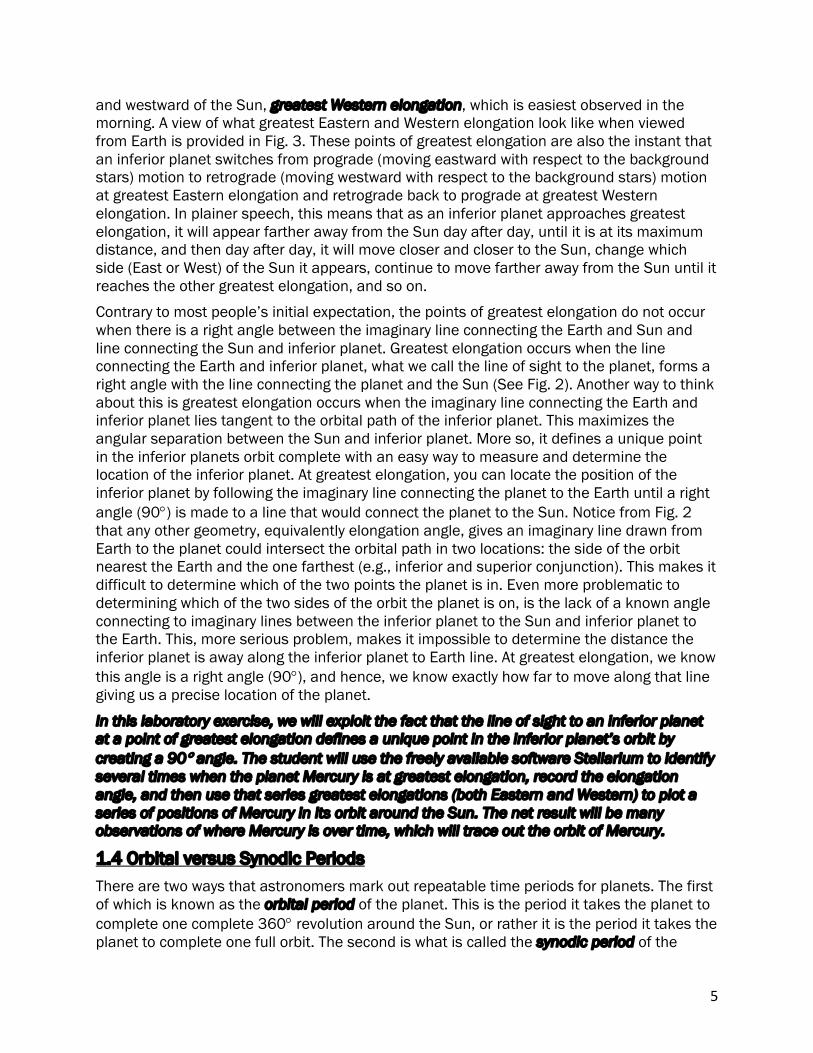
Two other important orbital geometries for the inferior planets are the two points where the planet appears as far away from the Sun as possible called greatest elongation. Elongation is the term astronomers use describe the angular separation between the Sun and the planet, and so greatest elongation occurs when the planet is as far away, angularly, from the Sun as it can be. There are two such elongations (see Fig. 2), where the planet is observed eastward of the Sun, greatest Eastern elongation, which is easiest observed in the evening,

Figure 2. Planetary geometries of note for inferior planets. The green circle represents Earth and the red circle the inferior planet. Their orbital paths and directions are indicated. The dashed gray lines represent arbitrary line of sight from Earth. The inferior planet appears farthest from the Sun (greatest elongation) at the indicated points.

Figure 3. Greatest Eastern and Western elongation as seen from an observer on Earth. When can be seen in the morning, it is West of the Sun, and when it seen in the evening it is East to the Sun. It’s maximum distance from the Sun marks greatest elongation.

5

and westward of the Sun, greatest Western elongation, which is easiest observed in the morning. A view of what greatest Eastern and Western elongation look like when viewed from Earth is provided in Fig. 3. These points of greatest elongation are also the instant that an inferior planet switches from prograde (moving eastward with respect to the background stars) motion to retrograde (moving westward with respect to the background stars) motion at greatest Eastern elongation and retrograde back to prograde at greatest Western elongation. In plainer speech, this means that as an inferior planet approaches greatest elongation, it will appear farther away from the Sun day after day, until it is at its maximum distance, and then day after day, it will move closer and closer to the Sun, change which side (East or West) of the Sun it appears, continue to move farther away from the Sun until it reaches the other greatest elongation, and so on.

Contrary to most people’s initial expectation, the points of greatest elongation do not occur when there is a right angle between the imaginary line connecting the Earth and Sun and line connecting the Sun and inferior planet. Greatest elongation occurs when the line connecting the Earth and inferior planet, what we call the line of sight to the planet, forms a right angle with the line connecting the planet and the Sun (See Fig. 2). Another way to think about this is greatest elongation occurs when the imaginary line connecting the Earth and inferior planet lies tangent to the orbital path of the inferior planet. This maximizes the angular separation between the Sun and inferior planet. More so, it defines a unique point in the inferior planets orbit complete with an easy way to measure and determine the location of the inferior planet. At greatest elongation, you can locate the position of the inferior planet by following the imaginary line connecting the planet to the Earth until a right angle (90°) is made to a line that would connect the planet to the Sun. Notice from Fig. 2 that any other geometry, equivalently elongation angle, gives an imaginary line drawn from Earth to the planet could intersect the orbital path in two locations: the side of the orbit nearest the Earth and the one farthest (e.g., inferior and superior conjunction). This makes it difficult to determine which of the two points the planet is in. Even more problematic to determining which of the two sides of the orbit the planet is on, is the lack of a known angle connecting to imaginary lines between the inferior planet to the Sun and inferior planet to the Earth. This, more serious problem, makes it impossible to determine the distance the inferior planet is away along the inferior planet to Earth line. At greatest elongation, we know this angle is a right angle (90°), and hence, we know exactly how far to move along that line giving us a precise location of the planet.

In this laboratory exercise, we will exploit the fact that the line of sight to an inferior planet at a point of greatest elongation defines a unique point in the inferior planet’s orbit by creating a 90° angle. The student will use the freely available software Stellarium to identify several times when the planet Mercury is at greatest elongation, record the elongation angle, and then use that series greatest elongations (both Eastern and Western) to plot a series of positions of Mercury in its orbit around the Sun. The net result will be many observations of where Mercury is over time, which will trace out the orbit of Mercury.

1.4 Orbital versus Synodic Periods There are two ways that astronomers mark out repeatable time periods for planets. The first of which is known as the orbital period of the planet. This is the period it takes the planet to complete one complete 360° revolution around the Sun, or rather it is the period it takes the planet to complete one full orbit. The second is what is called the synodic period of the

6

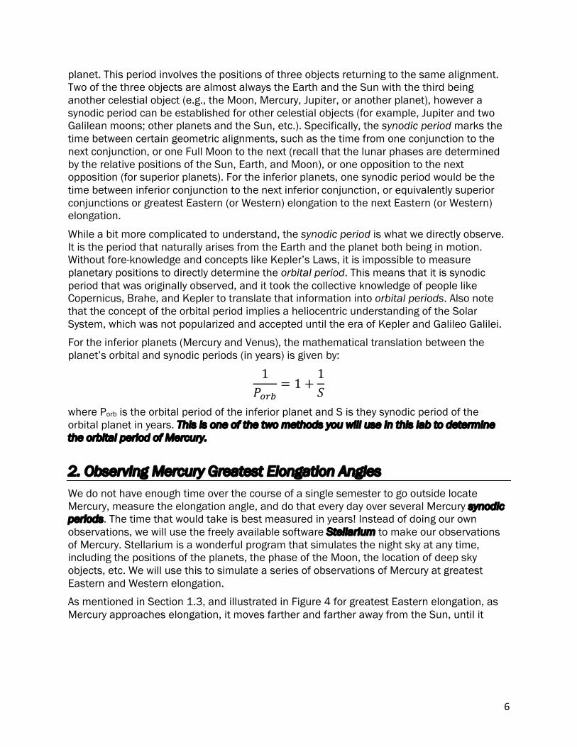
planet. This period involves the positions of three objects returning to the same alignment. Two of the three objects are almost always the Earth and the Sun with the third being another celestial object (e.g., the Moon, Mercury, Jupiter, or another planet), however a synodic period can be established for other celestial objects (for example, Jupiter and two Galilean moons; other planets and the Sun, etc.). Specifically, the synodic period marks the time between certain geometric alignments, such as the time from one conjunction to the next conjunction, or one Full Moon to the next (recall that the lunar phases are determined by the relative positions of the Sun, Earth, and Moon), or one opposition to the next opposition (for superior planets). For the inferior planets, one synodic period would be the time between inferior conjunction to the next inferior conjunction, or equivalently superior conjunctions or greatest Eastern (or Western) elongation to the next Eastern (or Western) elongation.

While a bit more complicated to understand, the synodic period is what we directly observe. It is the period that naturally arises from the Earth and the planet both being in motion. Without fore-knowledge and concepts like Kepler’s Laws, it is impossible to measure planetary positions to directly determine the orbital period. This means that it is synodic period that was originally observed, and it took the collective knowledge of people like Copernicus, Brahe, and Kepler to translate that information into orbital periods. Also note that the concept of the orbital period implies a heliocentric understanding of the Solar System, which was not popularized and accepted until the era of Kepler and Galileo Galilei.

For the inferior planets (Mercury and Venus), the mathematical translation between the planet’s orbital and synodic periods (in years) is given by:

1𝑃567

= 1 +1𝑆

where Porb is the orbital period of the inferior planet and S is they synodic period of the orbital planet in years. This is one of the two methods you will use in this lab to determine the orbital period of Mercury. 2. Observing Mercury Greatest Elongation Angles We do not have enough time over the course of a single semester to go outside locate Mercury, measure the elongation angle, and do that every day over several Mercury synodic periods. The time that would take is best measured in years! Instead of doing our own observations, we will use the freely available software Stellarium to make our observations of Mercury. Stellarium is a wonderful program that simulates the night sky at any time, including the positions of the planets, the phase of the Moon, the location of deep sky objects, etc. We will use this to simulate a series of observations of Mercury at greatest Eastern and Western elongation.

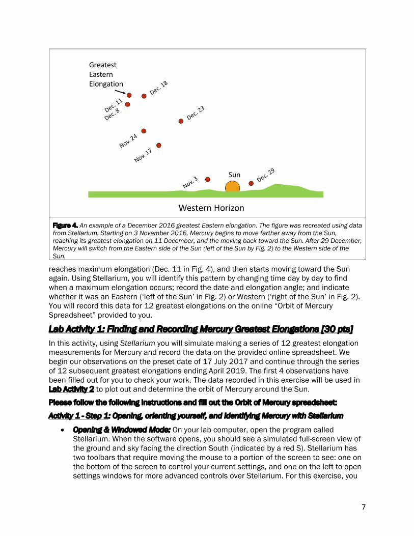
As mentioned in Section 1.3, and illustrated in Figure 4 for greatest Eastern elongation, as Mercury approaches elongation, it moves farther and farther away from the Sun, until it

7

reaches maximum elongation (Dec. 11 in Fig. 4), and then starts moving toward the Sun again. Using Stellarium, you will identify this pattern by changing time day by day to find when a maximum elongation occurs; record the date and elongation angle; and indicate whether it was an Eastern (‘left of the Sun’ in Fig. 2) or Western (‘right of the Sun’ in Fig. 2). You will record this data for 12 greatest elongations on the online “Orbit of Mercury Spreadsheet” provided to you.

Lab Activity 1: Finding and Recording Mercury Greatest Elongations [30 pts] In this activity, using Stellarium you will simulate making a series of 12 greatest elongation measurements for Mercury and record the data on the provided online spreadsheet. We begin our observations on the preset date of 17 July 2017 and continue through the series of 12 subsequent greatest elongations ending April 2019. The first 4 observations have been filled out for you to check your work. The data recorded in this exercise will be used in Lab Activity 2 to plot out and determine the orbit of Mercury around the Sun.

Please follow the following instructions and fill out the Orbit of Mercury spreadsheet:

Activity 1 - Step 1: Opening, orienting yourself, and identifying Mercury with Stellarium

• Opening & Windowed Mode: On your lab computer, open the program called Stellarium. When the software opens, you should see a simulated full-screen view of the ground and sky facing the direction South (indicated by a red S). Stellarium has two toolbars that require moving the mouse to a portion of the screen to see: one on the bottom of the screen to control your current settings, and one on the left to open settings windows for more advanced controls over Stellarium. For this exercise, you

Figure 4. An example of a December 2016 greatest Eastern elongation. The figure was recreated using data from Stellarium. Starting on 3 November 2016, Mercury begins to move farther away from the Sun, reaching its greatest elongation on 11 December, and the moving back toward the Sun. After 29 December, Mercury will switch from the Eastern side of the Sun (left of the Sun by Fig. 2) to the Western side of the Sun.

8

will want to work in a windowed-mode of Stellarium. Hover your mouse cursor over the bottom of the view to bring up Stellarium’s bottom toolbar. Click on the “Full-screen Mode” button to enter the windowed mode.

• Controlling Time: To keep all our observations at the same time of day, we need to pause Stellarium’s auto-advancing of time. Move your mouse to the bottom tool bar and click the 4button to pause time. Next move the mouse to the left of the screen to bring up the left toolbar. Select the “Date/Time” window to bring up the date and time controls. In the “Date and Time” window that opens, change the date to July 17, 2017 (2017/07/17) at noon-time (12:00:00). You should now be looking toward the South, and you should see bright blue skies. That daylight, however is blocking our view of Mercury.

• Turning Off the Atmosphere: To see Mercury during the daytime, we need to make use of Stellarium’s function that allows you to “turn off” Earth’s atmosphere. You can either press the letter ‘a’, or on the bottom toolbar, find and select the atmosphere toggle button (it looks like a cloud) and click on it to turn the effects of the atmosphere off. The sky should darken and you can now see the stars.

• Locating Mercury: The first step in finding Mercury is to turn on the planet labels in Stellarium. These might be already turned on depending on how your computer’s default settings are configured. If it is, the “Planet Labels” button on the bottom toolbar (it looks like Saturn) should be lit up. If they are not, however, click on the button to turn on the labels. Next, you need to locate Mercury. You can find Mercury one of two ways. You can locate Mercury by manually moving your view of the sky by clicking and holding down the left mouse button anywhere in the sky and moving the mouse to change your view. Hint: Mercury will be near the Sun (always less than 28 degrees). Once you locate Mercury, left-click on it to open the information display, which will be projected on the top left of the Stellarium window. Alternatively, you can find Mercury by opening the “Search Window” (or press F3) from the left toolbar, and searching for “Mercury”. The information display that appears contains a plethora of data on Mercury, including type of object, apparent magnitude, absolute magnitude, RA/Dec, phase, etc. We are only going to use a few of these pieces of information during this lab exercise, the most important of which is the elongation angle, which is the third piece of information from the bottom (above “illuminated” and “phase”).

Activity 1 - Step 2: Identifying and Recording Greatest Elongations

We are now ready to start measuring and finding the greatest elongations of Mercury. We are starting on July 17, 2017 at noon, which you will notice has Mercury on the Eastern side (“to the left of”; East is to the left of South) the Sun. Your elongation angle should read near to +23°34’17.6”, which reads as 23 degrees [°], 34 minutes [‘], and 17.6 seconds [“]. Recall from your lectures that there are 60 “minutes (of arc)” in one degree and 60 “seconds (of arc)” in one “minute.” We are now ready to advance time one day at a time to find the date when a greatest elongation occurs. In this case, we begin advancing toward greatest Eastern elongation.

9

• If you have closed your “Time and Date” window, reopen it. We will now advance time by one solar day at a time and watch for the time when Mercury reaches its farthest distance from the Sun, or greatest elongation. You can advance time by one solar day by either using the up arrow in the day part of the “Time and Date” window, or you can press the “=” key on your keyboard one time. When you advance time by one day to July 18, 2017 at noon, did Mercury move more eastward and a larger elongation angle or more westward, and to smaller elongation angle? If you are started at this lab’s default of July 17, 2017, moving forward by one day should have moved Mercury eastward to an elongation angle near +24°25’34.4”. Notice that the phase of Mercury slightly decreased as well, from 0.65 to 0.64, where phase equal to 1.0 is a “Full” Mercury and 0.0 is a “New” Mercury. Mercury is waning and heading toward its “New” phase.

• Continue to advance time one day at a time watching which direction Mercury is moving. Our goal is move one day at a time until we identify the day when maximum elongation occurs and then record that information on the “Orbit of Mercury Spreadsheet” provided to you for this lab. Pay careful attention to both Mercury’s location relative to the Sun and to the elongation angle data displayed in the information display. To find the greatest elongation will necessarily go past the date of greatest elongation, and need to go backwards in time by pressing the down button in the “Time and Date” window or pressing “-“ on your keyboard. Initially, we are heading toward our first greatest Eastern elongation, which will occur on July 30th with an elongation angle near +27°11’49.5”. Do you best to identify the day it occurs on your own because you will be responsible for independently identifying 8 greatest elongations on your own. The first four have been filled out for you so you can confirm your method of determining the time of greatest elongation.

• Record this date and elongation angle on your “Orbit of Mercury Spreadsheet.” The spreadsheet requires you to fill out the DATE column with the date that you observed greatest elongation; the ELONGATION ANGLE broken into three separate columns, DEG (degrees), MIN (minutes), and SEC (seconds), for easy conversion to degrees; and the DIRECTION of elongation as either E for greatest Eastern elongation and W for greatest Western elongation. All other columns will auto-populate as you record your data, including the calculation to determine: “Days Passed Since First Elongation”, “Days Since Last Elongation”, “Degrees Earth Moved Since Last Elongation”, and “Elongation in Degrees”. The first greatest elongation has been filled out for you as an example.

• Continue advancing time one day at a time (or perhaps one week at a time, by pressing “+”, once you are comfortable with identifying elongations). As you move through the days, take a few notes on how Mercury changes position from day to day, and compare that to the description in Section 1.3 and Fig. 4. Also, pay attention to how the angular size and phase of Mercury periodically change. Record the day and elongation angle of each of the next 14 greatest elongations on your “Orbit of Mercury Spreadsheet.” Pay attention to recording whether the greatest elongation is an Eastern (E) or a Western (W) elongation as this will be a critical piece of information for the next part of this lab exercise.

10

3. The Orbit of Mercury 3.1 Creating the Orbit of Mercury Lab Activity 2: Creating the Orbit of Mercury [30 pts]

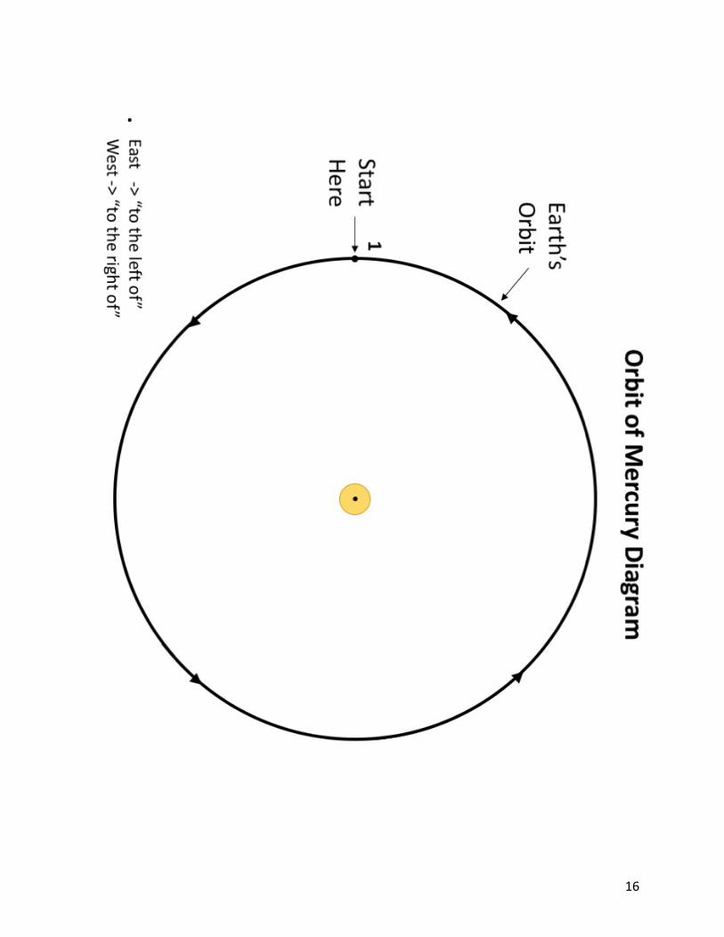
In this activity, you will use the data we recorded in your “Orbit of Mercury Spreadsheet” to plot out 12 positions of Mercury as it orbits the Sun on the “Orbit of Mercury Diagram” provided below on Page 17. To properly plot out the positions of Mercury to establish an estimate of its orbital path around the Sun, you will want to refer to Section 1.3 and Fig. 2 as we will be utilizing the unique geometric configuration between the Earth, Mercury, and the Sun to establish unique locations of Mercury in its orbit around the Sun.

This process is a repeatable algorithm of steps. If you keep each step of that algorithm in mind, and proceed one step at a time, you should be able to efficiently complete this exercise.

Activity 2 - Step 1: Draw a line connecting Earth to the Sun.

• The name of the instruction says it all. Beginning with our initial position of Earth indicated as point (1) and labeled with “Start Here” on your “Orbit of Mercury Diagram,” draw a line connecting the position of the Earth [point (1)] to the center of the Sun, indicated by the yellow sphere in the center of the diagram.

Activity 2 – Step 2: Note Eastern (E) or Western (W) elongation and draw a line of sight to Mercury

This step requires you to first note whether the greatest elongation you are dealing with is an Eastern (E) or a Western (W) one. As illustrated in Fig. 2, this will determine if you draw your line of sight along which Mercury falls “to the left of” in the case of greatest Eastern elongation, or “to the right of” in the case of greatest Western elongation.

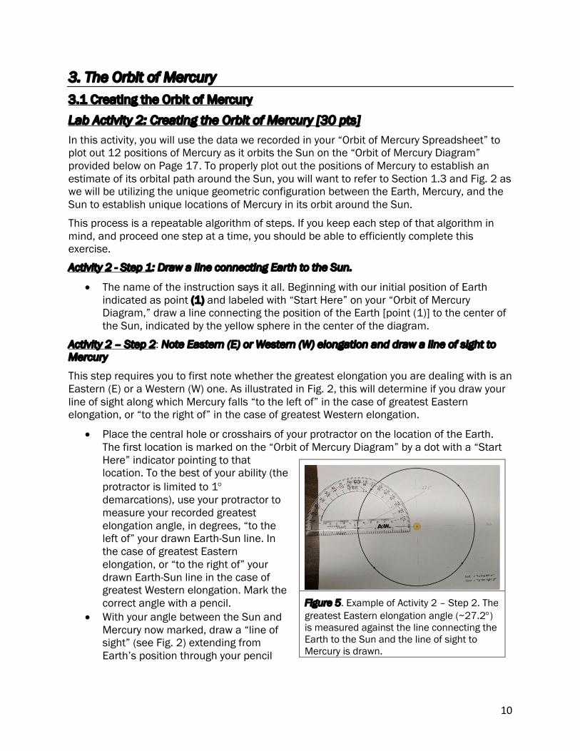
• Place the central hole or crosshairs of your protractor on the location of the Earth. The first location is marked on the “Orbit of Mercury Diagram” by a dot with a “Start Here” indicator pointing to that location. To the best of your ability (the protractor is limited to 1° demarcations), use your protractor to measure your recorded greatest elongation angle, in degrees, “to the left of” your drawn Earth-Sun line. In the case of greatest Eastern elongation, or “to the right of” your drawn Earth-Sun line in the case of greatest Western elongation. Mark the correct angle with a pencil.

• With your angle between the Sun and Mercury now marked, draw a “line of sight” (see Fig. 2) extending from Earth’s position through your pencil

Figure 5. Example of Activity 2 – Step 2. The greatest Eastern elongation angle (~27.2°) is measured against the line connecting the Earth to the Sun and the line of sight to Mercury is drawn.

11

mark that indicates the correct elongation angle. Due to the unique geometry related to greatest elongations, Mercury must lie somewhere along this line of sight!

• A picture demonstrating Activity 2 – Steps 1 & 2 is provided in Fig. 5.

Activity 2 – Step 3: Locating Mercury via a Right Angle

In this step, we will utilize the fact that during greatest elongation, there is a right angle (90°) between the line connecting Earth to Mercury and the line connecting Mercury to the Sun (See Fig. 2).

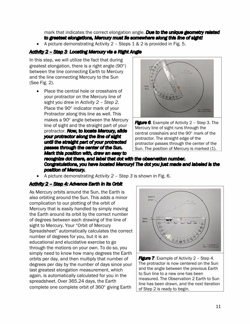
• Place the central hole or crosshairs of your protractor on the Mercury line of sight you drew in Activity 2 – Step 2. Place the 90° indicator mark of your Protractor along this line as well. This makes a 90° angle between the Mercury line of sight and the straight part of your protractor. Now, to locate Mercury, slide your protractor along the line of sight until the straight part of your protracted passes through the center of the Sun. Mark this position with, draw an easy to recognize dot there, and label that dot with the observation number. Congratulations, you have located Mercury! The dot you just made and labeled is the position of Mercury.

• A picture demonstrating Activity 2 – Step 3 is shown in Fig. 6.

Activity 2 – Step 4: Advance Earth in its Orbit

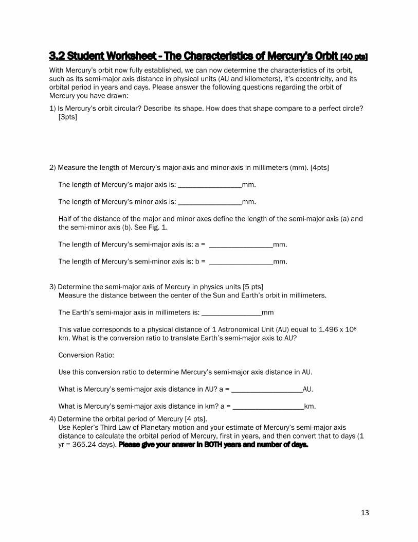
As Mercury orbits around the Sun, the Earth is also orbiting around the Sun. This adds a minor complication to our plotting of the orbit of Mercury that is easily handled by simply moving the Earth around its orbit by the correct number of degrees between each drawing of the line of sight to Mercury. Your “Orbit of Mercury Spreadsheet” automatically calculates the correct number of degrees for you, but it is an educational and elucidative exercise to go through the motions on your own. To do so, you simply need to know how many degrees the Earth orbits per day, and then multiply that number of degrees per day by the number of days since your last greatest elongation measurement, which again, is automatically calculated for you in the spreadsheet. Over 365.24 days, the Earth complete one complete orbit of 360° giving Earth

Figure 6. Example of Activity 2 – Step 3. The Mercury line of sight runs through the central crosshairs and the 90° mark of the protractor. The straight edge of the protractor passes through the center of the Sun. The position of Mercury is marked (1).

Figure 7. Example of Activity 2 – Step 4. The protractor is now centered on the Sun and the angle between the previous Earth to Sun line to a new one has been measured. The Observation 2 Earth to Sun line has been drawn, and the next iteration of Step 2 is ready to begin.

12

moving (360° ÷ 365.24 days) = 0.986 degrees per day. Hence, in a period of about 44 days, the Earth has revolved counter-clockwise around the Sun, 44 days ´ 0.986°/day = 43.37°, or about 43°, from its previous location.

On your “Orbit of Mercury Diagram” the Earth is orbiting the Sun in a counter-clockwise direction meaning we are looking down on the North pole of the Sun and Earth. This is the direction we need to move Earth to find the location of Earth at the next greatest Elongation of Mercury.

• Place the central hole or crosshairs of your protractor on the center of the Sun. Arrange the protractor such that the 0° mark passes through the previous Earth to Sun line you drew.

• To the best of your ability measure out the number of degrees the Earth has moved since the previous greatest Elongation of Mercury. This number is calculated and highlighted in blue text for you in the “Degrees Earth Moved Since Last Elongation” column of your “Orbit of Mercury Spreadsheet. Mark that angle on your “Orbit of Mercury Diagram”. Now use your straight edge to draw a line from the center of the Sun, though that mark, to the edge of Earth’s orbit. This indicates where Earth should be at the next greatest elongation of Mercury. LABEL THAT POINT WITH THE NUMBER OF THE OBSERVATION. For example, if this is your first advancement of Earth after starting at “Start Here”, then label this position of Earth as 2.

• The line you have just drawn between the Sun and the new position of the Earth is your new Earth to Sun line for your next elongation observation.

• A picture demonstrating Activity 2: Step 4 is provided in Fig. 7

Activity 2 – Repeat Steps 2 through 4

With the new position of Earth clearly marked and the new Earth to Sun line drawn (Step 1), you are now ready to repeat Steps 2 through 4 for all your observations on the “Orbit of Mercury Spreadsheet.” Each new round through Steps 2 – 4 will give you a new position of Mercury in its orbit giving you a total of 12 positions of Mercury, which is enough to establish the orbit of Mercury.

Activity 2 – Step 5: Tracing the and labeling the Orbit of Mercury

By this point, you should have marked and labeled 12 orbital positions of Mercury. Now all that is left to do to establish Mercury’s orbital path is to connect dots.

• To the best of your ability, connect dots 1 – 12 that indicate Mercury’s positions. This is tracing out the orbit of Mercury. Keep in mind that we know orbits are elliptical in shape, so your lines should be smooth and arc slightly between the points.

• Using your straight edge, search for the longest possible line that goes through the center of the Sun and connects two opposite edges of Mercury’s orbit. This line will be Mercury’s major axis (see Fig. 1). Record the length of this line on the answer in the answer sheet (Section 3.2: Student Worksheet) provided to you for this lab. Half of this value is Mercury’s semi-major axis length.

• At the center of your major axis, draw a line connecting opposite edges of Mercury’s orbit that is at a right angle to your semi-major axis. This is Mercury’s minor axis. Record the length of this line on the answer sheet provided to you for this lab. Half of this value is Mercury’s semi-minor axis length.

13

3.2 Student Worksheet - The Characteristics of Mercury’s Orbit [40 pts] With Mercury’s orbit now fully established, we can now determine the characteristics of its orbit, such as its semi-major axis distance in physical units (AU and kilometers), it’s eccentricity, and its orbital period in years and days. Please answer the following questions regarding the orbit of Mercury you have drawn:

1) Is Mercury’s orbit circular? Describe its shape. How does that shape compare to a perfect circle? [3pts]

2) Measure the length of Mercury’s major-axis and minor-axis in millimeters (mm). [4pts] The length of Mercury’s major axis is: _________________mm. The length of Mercury’s minor axis is: _________________mm. Half of the distance of the major and minor axes define the length of the semi-major axis (a) and the semi-minor axis (b). See Fig. 1. The length of Mercury’s semi-major axis is: a = _________________mm. The length of Mercury’s semi-minor axis is: b = _________________mm.

3) Determine the semi-major axis of Mercury in physics units [5 pts] Measure the distance between the center of the Sun and Earth’s orbit in millimeters. The Earth’s semi-major axis in millimeters is: ________________mm This value corresponds to a physical distance of 1 Astronomical Unit (AU) equal to 1.496 x 108 km. What is the conversion ratio to translate Earth’s semi-major axis to AU? Conversion Ratio: Use this conversion ratio to determine Mercury’s semi-major axis distance in AU. What is Mercury’s semi-major axis distance in AU? a = ___________________AU. What is Mercury’s semi-major axis distance in km? a = ___________________km.

4) Determine the orbital period of Mercury [4 pts]. Use Kepler’s Third Law of Planetary motion and your estimate of Mercury’s semi-major axis distance to calculate the orbital period of Mercury, first in years, and then convert that to days (1 yr = 365.24 days). Please give your answer in BOTH years and number of days.

14

5) Determine the eccentricity of Mercury [3 pts]. Use the equation for eccentricity given in Section 1.2 to calculate the eccentricity of Mercury’s orbit. You can use any measurement of semi-major and semi-minor axes that you have determined, but be sure to make sure the units match. The eccentricity of Mercury is, e = ____________________.

6) Determine the perihelion and aphelion distances [4 pts]. Use the equations for perihelion and aphelion distance given in Section 1.2. Please calculate these distances in AU and kilometers. Mercury’s aphelion distance is: aphelion distance = ______________________ AU

=______________________ km

perihelion distance = ______________________ AU

= ______________________ km

7) Determine the synodic period of Mercury using two different methods [4 pts].

Method 1: Use your “Orbit of Mercury Spreadsheet” to determine how days pass from each greatest Eastern elongation to the next. You should have 7 values. Average these 7 values together to determine an estimate of Mercury’s synodic value.

Write 7 independent estimates HERE:

What is the average of those 7 estimates? Your estimate of Mercury’s synodic period is…

Recall by definition, the synodic period of an object is the time it takes for it to return to the same geometric configuration (e.g., one greatest Eastern elongation to the next), so each one of the seven values is an independent estimation of the synodic period. While each independent estimate may have large error (be far from the true value), an average of many measurements will quickly approach the actual value of Mercury’s synodic period. Method 2: Use the equation in Section 1.4 that relates orbital period to synodic period to determine Mercury’s synodic period, S, using your determination of Mercury’s orbital period from Question 4. Note this equation requires the periods to be in years. You will have to convert to days.

Mercury’s synodic period is, S = _________________ days

15

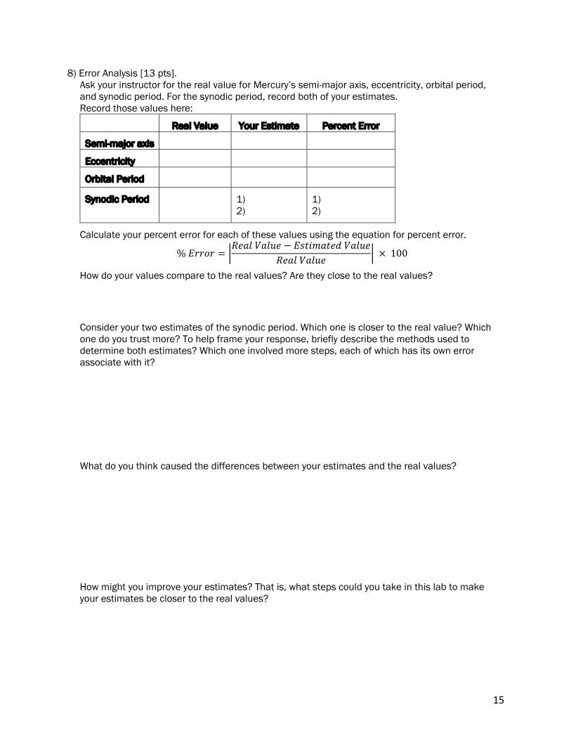
8) Error Analysis [13 pts]. Ask your instructor for the real value for Mercury’s semi-major axis, eccentricity, orbital period, and synodic period. For the synodic period, record both of your estimates. Record those values here:

Real Value Your Estimate Percent Error

Semi-major axis

Eccentricity

Orbital Period

Synodic Period 1) 2)

1) 2)

Calculate your percent error for each of these values using the equation for percent error.

%𝐸𝑟𝑟𝑜𝑟 = ;𝑅𝑒𝑎𝑙𝑉𝑎𝑙𝑢𝑒 − 𝐸𝑠𝑡𝑖𝑚𝑎𝑡𝑒𝑑𝑉𝑎𝑙𝑢𝑒

𝑅𝑒𝑎𝑙𝑉𝑎𝑙𝑢𝑒; × 100

How do your values compare to the real values? Are they close to the real values?

Consider your two estimates of the synodic period. Which one is closer to the real value? Which one do you trust more? To help frame your response, briefly describe the methods used to determine both estimates? Which one involved more steps, each of which has its own error associate with it?

What do you think caused the differences between your estimates and the real values?

How might you improve your estimates? That is, what steps could you take in this lab to make your estimates be closer to the real values?

16

.