LAKEHEAD UNIVERSITY

DEPARTMENT OF GEOGRAPHY

LAB MANUAL

for

GEOG/ENST 2331

CLIMATOLOGY

Fall 2015

Prepared by

Dr. Adam Cornwell

Jason Freeburn

Graham Saunders

Thunder Bay, Ontario

January, 2018

ii

Table of Contents

Winter 2018 Course Outline for GEOG/ENST 2331 .................................... 1

Section 1: Diagrams for Labs .......................................................................... 2

Exhibit 1: Geostrophic Winds ............................................................................................... 3

Exhibit 2: Gradient Winds ..................................................................................................... 4

Exhibit 3: Surface Winds ...................................................................................................... 5

Exhibit 4: Saturation Vapour Pressure .................................................................................. 6

Exhibit 5: Adiabatic Cooling .................................................................................................. 7

Exhibit 6: Saturated Adiabatic Lapse Rates .......................................................................... 8

Exhibit 7: Vertical Stability Analysis ...................................................................................... 9

Exhibit 8: Pressure Belts And Global Air Circulation Systems ............................................ 10

Exhibit 9: Cold Front ........................................................................................................... 11

Exhibit 10: Warm Front ....................................................................................................... 12

Exhibit 12: Warm Occluded Front ....................................................................................... 14

Exhibit 13: Mature Stage Cyclone ...................................................................................... 15

Exhibit 14: Cyclone Occlusion ............................................................................................ 16

Section 2: Lab Exercises ................................................................................ 17

Lab 0: Mathematics and Climatology .................................................................................. 18

0.1 Background ..................................................................................................................... 18

0.2 Significant digits and the use of scientific notation ........................................................ 18

0.3 Units and the SI system .................................................................................................. 19

0.4 Practice with digits and units .......................................................................................... 21

0.5 Arithmetic with large numbers ....................................................................................... 22

0.6 Practice with large numbers ............................................................................................ 23

0.7 Re-arranging equations to solve for unknowns .............................................................. 23

0.8 Practice solving equations with one unknown variable .................................................. 24

Lab 1: Global Energy Budgets ............................................................................................ 25

1.1 Background ............................................................................................................... 25

1.2 Objectives of this exercise ........................................................................................ 25

1.3 Calculating the Effective Radiative Temperature ..................................................... 25

iii

1.4 Exercises for Effective Radiative Temperatures ....................................................... 28

1.5 Incorporation of the Greenhouse Effect .................................................................... 29

1.6 Exercises for a Single Layer Atmosphere ................................................................. 31

Lab 2: Isotherms and Isobars ............................................................................................. 31

2.1 Isotherm background ................................................................................................ 32

2.2 Interpolation of isotherms ......................................................................................... 32

2.3 Isotherm exercises ..................................................................................................... 34

2.4 Isobar background ..................................................................................................... 34

2.5 Sea-level pressure ..................................................................................................... 34

2.6 Interpolation of isobars ............................................................................................. 35

2.7 Isobar Exercises ........................................................................................................ 36

Lab 3: Atmospheric Mechanics .......................................................................................... 37

3.1 Background ............................................................................................................... 37

3.2 Modelling atmospheric mechanics ........................................................................... 37

3.3 Exercises ................................................................................................................... 39

Lab 4: Adiabatic Lapse Rates ............................................................................................. 41

4.1 Types of adiabatic cooling and heating .................................................................... 41

4.2 Orographic rainfall and Chinooks ............................................................................. 41

4.3 DALR vs. SALR ....................................................................................................... 42

4.4 Data for demonstration: The following data are for class demonstration only ......... 43

LAB 4 – ADIABATIC LAPSE RATES................................................................... 44

4.5 Data for class assignment (will be provided) ............................................................ 45

Lab 5 Quiz: Atmospheric Stability ....................................................................................... 46

5.1 Meaning of stability .................................................................................................. 46

5.2 General criteria for determining atmospheric stability ............................................. 46

5.3 Stability analysis: Graphic method and calculation .................................................. 47

5.4 In-Class Test on an example of the above calculations of stability analysis ............ 52

Lab 6: Weather Observation............................................................................................... 54

6.1 Objective of the exercise ........................................................................................... 54

6.2 Data ........................................................................................................................... 54

iv

6.3 Collecting Observations and Performing Calculations in Excel ............................... 56

6.4 Tasks ......................................................................................................................... 58

6.5 Lab Report ................................................................................................................ 63

Lab 7: Slate Islands Tourism .............................................................................................. 64

7.1 Objective ......................................................................................................................... 64

7.2 Background: The Slate Islands ....................................................................................... 64

7.3 The Tour ......................................................................................................................... 68

P a g e | 1

Winter 2018 Course Outline for GEOG/ENST 2331

Instructor: Graham Saunders Office: TBA graham.saunders@lakeheadu.ca

Lab Instructor: Jason Freeburn Office: RC 2004 jason.freeburn@lakeheadu.ca

Course Objectives

This course gives a general introduction to meteorology and climatology. Meteorology topics include

energy balance in the atmosphere, moisture and cloud development in the atmosphere, atmospheric

dynamics, small and large scale circulations, storms and cyclones, and weather forecasting. Climatology

topics include the interaction between the atmosphere and oceans over long time periods, climate

classification, and the potential for climatic change.

Text: Ahrens, Jackson and Jackson, 2016.Meteorology Today, 2nd

Canadian Edition (Nelson Education).

Manual: Cornwell, Freeburn, and Saunders 2018. Climatology Manual.

Evaluation Scheme and Schedule:

Lab 0 Jan. 16/18 0

Lab 1 Jan. 23/25 5

Lab 2 Jan. 30/Feb. 1 5

Lab 3 Feb. 6/8 5

Midterm Feb. 14 20

Lab 4 Feb. 27/Mar. 1 5

Lab 5 – Lab Quiz Mar. 6/8 7

Lab 7 Mar. 13/15 8

Lab 6 – Group Project* Mar. 20/22 & Mar. 27/29 5

Final Examination TBA 40

Lecture Times and Place

Monday and Wednesday: 8:30 – 9:30 (RC 2003)

Lab Times and Place

Tuesday: 10:30 – 12:30 / Thursday: 2:30 – 4:30 (RC 2003)

*Lab 6 sessions will be in ATAC 3009

P a g e | 2

Section 1: Diagrams for Labs

The attached diagrams are intended as teaching/study aids for the lab exercises and should,

therefore, be used for developing your notes. You should consider making notes directly on the

spaces between the graphics and/or on the back pages. Some test questions may be based on

these diagrams, in addition to those used in lectures.

P a g e | 3

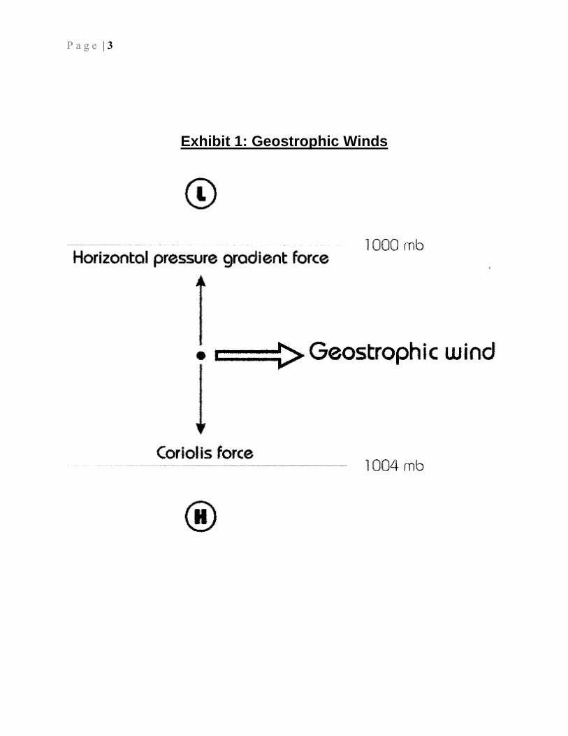
Exhibit 1: Geostrophic Winds

P a g e | 4

Exhibit 2: Gradient Winds

P a g e | 5

Exhibit 3: Surface Winds

P a g e | 6

Exhibit 4: Saturation Vapour Pressure

P a g e | 7

Exhibit 5: Adiabatic Cooling

P a g e | 8

Exhibit 6: Saturated Adiabatic Lapse Rates

P a g e | 9

Exhibit 7: Vertical Stability Analysis

P a g e | 10

Exhibit 8: Pressure Belts And Global Air Circulation Systems

P a g e | 11

Exhibit 9: Cold Front

P a g e | 12

Exhibit 10: Warm Front

P a g e | 13

Exhibit 11: Cold Occluded Front

P a g e | 14

Exhibit 12: Warm Occluded Front

P a g e | 15

Exhibit 13: Mature Stage Cyclone

P a g e | 16

Exhibit 14: Cyclone Occlusion

P a g e | 17

Section 2: Lab Exercises

P a g e | 18

Lab 0: Mathematics and Climatology

0.1 Background

The study of climatology is largely quantitative. While much can be learned from simple

comparative work (e.g. oceans warm and cool more slowly than continents, or mountains receive

more rainfall than plains), a thorough appreciation of the processes involved is best achieved by

working through mathematical models and arriving at conclusions that are quantitative as well as

qualitative. Several of the exercises in this manual, therefore, use mathematical equations to

model real processes from the physical world.

Not all students enrolled in 2331 have a strong background in math, and many are out of practice

in the techniques used in this manual. This lab exercise is intended to re-introduce techniques

that will be important for this course and provide a reference for later work.

0.2 Significant digits and the use of scientific notation

An important consideration in science is measurement accuracy. No measurement can possibly

be 100% precise. There must always be consideration for error and the physical limitations of the

measurement instrument. Therefore, it is important when we transform observations with

mathematical equations that we don’t end up pretending to suddenly have more accuracy than we

started with. Consider the following calculation:

52.1398002801.70.15

The input values (15.0 and 7.01) have clearly defined limits to their accuracy: three digits each.

The output, however, is proclaiming ten digits of accuracy. This is a lie. Strictly speaking, we

cannot know the result with any more accuracy than we know the input values. Therefore, we

should round the result to three significant digits: 2.14. To simplify things for this course, we

will assume that all calculations should be done with three significant digits.

P a g e | 19

The significant digits of a number are generally easy to count. There may be confusion, however,

in the case of ‘placeholder’ zeroes. The number 700, for example, would be generally considered

to have just one significant digit (the seven). The zeroes are only there to put the seven in the

hundreds column instead of the ones column. But what if we do know this result is accurate to

three digits; i.e. it is less than 701 and more than 699?

This is one reason that scientists often turn to scientific notation. Scientific notation uses powers

of 10 rather than zeros to indicate how far the significant digits are from the ones column. 700 in

decimal notation is written as 7102 in scientific notation. If the value is known with three digits

of accuracy, it can be written as 7.00102 with no ambiguity.

Scientific notation is also very useful in representing very large or very small numbers, where

there would otherwise be a lot of placeholder zeroes to count. For example, 6.5 billion can be

written either as 6500000000 or as 6.5109. Very small numbers can be represented by using

negative powers of 10 (note that multiplying by 10-2

is equivalent to dividing by 102), so six

millionths can be written as 0.000006 or 610-6

. Each power of 10 is referred to as an order of

magnitude.

0.3 Units and the SI system

Units are a key part of any measurement. Statements like “It’s thirty degrees out,” or “Gas is up

to one twenty-seven,” only make sense if there is a general convention that temperature is

measured in Celsius and gasoline is priced in cents/litre. In a scientific context like climatology

the units must be included with any quantity, as there is more than one unit commonly used for

many types of measurements. A number without a unit is just a number.

Most commonly in scientific applications, both in Canada and (to a great extent) the United

States, the units used are from the Système International (SI) standard. This standard is based on

the metric system and makes use of the metric prefixes for converting to larger and smaller

P a g e | 20

scales of measurement. Scientific notation becomes very useful for scale conversions in the SI

system, as shown in Table 0.1, and also Appendix A of Ahrens et al.

Table 0.1: Scale Prefixes in SI

Symbol Prefix Factor Number Description

n nano 10-9

0.000000001 One-billionth

micro 10-6

0.000001 One-millionth

m milli 10-3

0.001 One-thousandth

c centi 10-2

0.01 One-hundredth

d deci 10-1

0.1 One-tenth

None 100

1 One

h hecto 102

100 One hundred

k kilo 103

1 000 One thousand

M mega 106

1 000 000 One million

G giga 109

1 000 000 000 One billion

The ‘Factor’ column illustrates that scientific notation can make prefix conversions in SI very

simple. 6.7103 m is equal to 6.7 km.

In the SI system, there is a base unit with no prefix for each type of measurement; for example,

the base unit for mass is the gram. However, there is also a unit that, by convention, is the most

commonly used unit for physical equations. This is referred to as the MKS system, as it is based

around metres, kilograms, and seconds. Converting measurements to the MKS system before

plugging them into equations can save a lot of difficult work after the fact to figure out the

appropriate units of the solution. The MKS units for the quantities used in climatology are given

in Table 0.2, along with other units that are often encountered, and also Table A.1 of Ahrens et

al.

P a g e | 21

Table 0.2: SI units and their symbols

Quantity Name MKS Other common units

Length metre m km, cm, mm

Mass (m) kilogram kg tonne, gram

Time (t) second s hour, day, year

Temperature (T) kelvin K Celsius

Density () kilogram per cubic

metre

kg m-3

Force (F) newton N

Pressure (P) pascal Pa hPa, kPa, bar, mbar

Velocity (u,v) metre per second m s-1

km h-1

, knots

Energy (E) joule J N m

Power watt W J s-1

0.4 Practice with digits and units

1. Convert the following numbers to scientific notation:

a. 3200

b. 6574000

c. 0.0000325

2. Convert the following numbers to decimal notation:

a. 6.37106

b. 1.5×1011

c. 5.6710-8

P a g e | 22

3. Convert the following quantities to their MKS units, in both decimal and scientific

notation:

a. A wavelength of 0.5 m

b. A speed of 300000 km/s

c. Atmospheric pressure of 1000 hPa

d. Atmospheric pressure of 1 bar

e. 46 mm of precipitation

f. Air temperature of 30C

0.5 Arithmetic with large numbers

Scientific notation requires special rules for things like addition and multiplication.

Understanding these rules can make performing these operations on large numbers simpler and

reduce the chance of making mistakes.

Scientific notation represents a number in the form a 10b, where a is the coefficient and b is the

exponent. For addition and subtraction, both numbers must first be expressed with the same

exponent. Then, the coefficients can simply be added (or subtracted) with no further exponent

change. For example:

2109 + 210

9 = 410

9

51010

+ 4108 = 510

10 + 0.0410

10 = 5.0410

10

For multiplication, the coefficients are multiplied, and the exponents are added together. For

division, the coefficients are divided and the exponent in the denominator is subtracted from the

exponent in the numerator. For example:

2109 310

9 = 610

18 (2 3 = 6 and 9 + 9 = 18)

51010

/ 4108 = 1.2510

2 (5 / 4 = 1.25 and 10 – 8 = 2)

P a g e | 23

0.6 Practice with large numbers

1. Given that the radius of the Earth is r = 6.37 × 106 m, calculate the surface area of the

Earth using the formula Area = 4r2.

2. Find the pressure gradient between two locations by dividing the difference in pressure

(9.8102 Pa) by the horizontal distance (1.210

3 km). Then, put your answer in MKS

units of Pa/m.

0.7 Re-arranging equations to solve for unknowns

The unknown variable in an equation is solved for by re-arranging the equation to isolate that

variable. This is done using the principle that if both sides of the equation are equal, then they

will remain equal if the same operation is performed on both sides (addition, subtraction,

multiplication, division; even exponents or trigonometric functions). For example, consider the

Ideal Gas Law:

TCP (0.1)

If the pressure is P = 1.0105 Pa, the temperature is T = 285 K, and the gas constant for air is C =

287 N m kg-1

K-1

(all MKS units), then the density () can be calculated by dividing both sides

by TC, thereby isolating .

3-1

4

555

m kg 22.110122.0101795.8

1000.1

81795

1000.1

287285

1000.1

TC

P

TC

TC

TC

P

If you have two equations and two unknown variables, the same approach can be used –

although you will not need to do it for this course. The key is to find a way to isolate one

unknown variable into one equation. See Lab 1 for an example of this approach.

P a g e | 24

0.8 Practice solving equations with one unknown variable

1. If a net force (F) of 100 N is applied to an object with a mass (m) of 20 kg, find the

acceleration (a) of that object using Newton’s second law of motion:

maF

(note: for MKS units of acceleration, 1 N kg-1

= 1 m s-2

)

2. Solve for the temperature (T) in Wien’s equation:

Tm

2897 given that m = 10 m and the constant is 2897 m K.

3. Solve for the emissivity () in the Stefan-Boltzmann equation:

4TI I = 400 W m-2

= 5.6710-8

W m-2

K-4

T = 300 K

P a g e | 25

Lab 1: Global Energy Budgets

1.1 Background

Recommended reading: Ahrens et al. Chapter 2.

The climatology of our planet is driven by radiant energy received from the Sun (insolation). In a

steady state, Earth’s energy budget will be a balance between radiation received and radiation

emitted. The reflection, absorption and emission of radiation are complicated by the presence of

an atmosphere that participates in all three processes.

The clouds in the atmosphere contribute greatly to the planetary albedo, increasing the amount of

insolation that is reflected back into space. Clouds, along with greenhouse gases, also absorb

longwave radiation that is emitted from the surface, heating the atmosphere. In turn, the

atmosphere emits radiation, but it does so in both directions so that some of this energy is

returned to the surface rather than being lost to space.

1.2 Objectives of this exercise

In this lab exercise you will explore relationships in the planetary energy budget by examining

the effects of changes in the boundary conditions. Other planets, stars and earlier time periods on

Earth are examples of systems that are governed by the same physical theories but with very

different climatological results. Climatologists study these examples in order to gain a better

understanding of our own climate system and its sensitivity to changes in atmospheric

composition.

1.3 Calculating the Effective Radiative Temperature

Celsius to Kelvin conversion 0oC = 273.15 K

Stefan-Boltzmann Law I = εσT4 (1.1)

Stefan-Boltzmann constant σ = 5.67 x 10-8

Wm-2

K-4

Wien's Law λm = 2897 / T (1.2)

P a g e | 26

Wien’s constant 2897 m K-1

Temperature of Sun Ts = 5800 K

Radius of Sun rs = 6.96 × 108 m

Distance between Sun and Earth dse = 1.5 × 1011

m

Radius of Earth re = 6.37 × 106 m

Albedo of Earth A = 0.3

There are four steps to calculating Earth’s energy budget:

Step 1: The energy emitted by the Sun.

Step 2: The energy received by Earth.

Step 3: The energy absorbed by Earth.

Step 4: The energy emitted by Earth.

Step 1:

The total irradiance (in watts) coming from the Sun can be calculated as:

Rs = εσ Ts4 × 4πrs

2 (1.3)

= 3.91 × 1026

W

where Ts is the temperature of the Sun and rs is the radius of the Sun. The Sun is a blackbody, so

the emissivity = 1.

Step 2:

This solar radiation is spread out over a sphere at the distance of Earth’s orbit. Earth’s shadow

area (a circle with the planet’s radius) represents a tiny fraction of that sphere. This fraction of

the total irradiance is intercepted by Earth.

P a g e | 27

Figure 1.1: Diagram showing the shadow area of a spherical planet

The fraction is:

10

2

2

1051.4

4

se

e

d

rF

(1.4)

where re is the radius of Earth and dse is the distance from the Sun to the Earth (the radius of a

sphere at the distance of Earth’s orbit).

The amount of energy received by Earth is this fraction of the total irradiance:

Re = Rs × F (1.5)

= 1.76 × 1017

W

Step 3:

Total Solar Irradiance (S) is the intensity of radiation per square metre received by Earth:

2-

2

Wm1380

e

e

r

RS

(1.6)

The intensity of insolation absorbed by Earth is reduced by the albedo:

P a g e | 28

Iin = S(1 – A) (1.7)

= 967 Wm-2

Step 4:

Earth absorbs radiation across a circular area facing the Sun. It emits radiation across the entire

area of its surface. Therefore, the intensity of radiation emitted from Earth can be calculated

from:

2-

22

Wm 75.2414

4

inout

eoutein

II

rIrI

(1.8)

The Stefan-Boltzman Law can then be used to determine the effective radiative temperature of

Earth:

4

1

out

e

IT (1.9)

= 255 K

where Earth is also a blackbody with emissivity = 1.

1.4 Exercises for Effective Radiative Temperatures

For this assignment please use the attached worksheet at the back of the manual.

1. The radius of Earth is roughly four times as big as the Moon. Both bodies are the same

distance from the Sun and have similar effective radiative temperatures (For this question,

we’ll say 255 K for both). Consider equations (1.3) and (1.2):

a. Which celestial body emits more radiation, and by how much (as a relative value,

e.g., twice as much, ten times as much…you do not need to calculate the actual

amount to answer this question; just consider the equation carefully)?

P a g e | 29

b. What is the wavelength of peak emission for each?

2. The “Dog Star”, Sirius A, is the brightest star in the night sky. It is an ‘A-type’ star; a larger

and hotter star than our Sun. Its radius is 1.20109 m, and its effective surface temperature is

10000 K. Treat it as a blackbody.

a. Following Step 1 (above), what is the total irradiance for Sirius A (in W)?

b. If our Sun were replaced by Sirius A, what would the radius of Earth’s orbit need to

be in order to maintain the same effective radiative temperature that is has now, i.e.

255 K? Hint: for this to happen, the amount of incoming radiation, Re, needs to be

the same as in Step 2 (above).

1.5 Incorporation of the Greenhouse Effect

The average surface temperature of the planet is significantly warmer than the effective radiative

temperature; 288 K as compared to 255K. The 33 degree difference is the result of the

greenhouse effect of the atmosphere. Longwave radiation emitted by the surface is absorbed by

greenhouse gases and clouds, heating the atmosphere. The atmosphere then radiates both up to

space and back to the surface, and the portion that is returned to the surface is the cause of higher

temperatures.

A simple approach to incorporating the greenhouse effect is to consider a one layer model of the

atmosphere. We can assume that it absorbs 10% of the incoming solar (shortwave) radiation (so

90% passes through to the surface) and 80% of the outgoing terrestrial (longwave) radiation (so

20% passes through to space). Here we will use I as the intensity of total incoming and outgoing

radiation, spread over the surface area of the planet; x will be the intensity emitted from the

surface and y will be the intensity emitted from the atmosphere in each direction.

P a g e | 30

Figure 1.2: Single layer atmosphere energy balance.

Assuming a steady state, the transfers at the top and bottom of the atmosphere must both be in

balance. Assuming I = 241.75 Wm-2

, as calculated above, we can identify the following two

relationships:

Surface: 0.9I = x – y

Space: I = 0.2x + y

Since both of these must be true, we can add the left-hand and right-hand sides together and they

will still be equal:

xI

xI

x + y. x - y + I + I .

2.1

9.1

2.19.1

2090

Therefore 8.38275.2412.1

9.1x Wm

-2 and y = I – 0.2x = 165.2 Wm

-2.

P a g e | 31

Using the Stefan-Boltzmann Law (1.1) for surface temperature, 4

1

xTe = 286.6 K. This is a

much closer estimate to the observed average surface temperature.

1.6 Exercises for a Single Layer Atmosphere

3. It is believed that in the Archean eon (2.5 billion years ago) the Sun’s radiative output was

30% less than it is today. That is, the total solar irradiance was

Rs = (1 – 0.3) × 3.91 × 1026

= 2.73×1026

W (1.10)

It follows from Steps 2-4 in Section 1.3 (you can check it if you’d like) that the intensity of

incoming and outgoing radiation (spread over the planet’s surface) would be similarly

reduced so that

I = (1 – 0.3) 241.75 = 169.23 Wm-2

(1.11)

a. If we assume the radius of the Sun was the same, and that the Earth’s atmosphere

was the same as it is now, solve the equations in Section 1.5 with that old value of

I to estimate the average surface temperature of the Earth using a single layer

atmosphere.

b. In fact, the Earth’s atmosphere was drastically different during the Archean eon

(15-20% CO2, 0% O2). Adjust the model in Section 1.5 so that the single-layer

atmosphere absorbs 10% of incoming radiation but 99% of outgoing radiation.

Label the radiation fluxes in Figure 1.3. What would be the temperature of the

early Earth surface and its atmosphere?

Figure 1.3

P a g e | 32

Lab 2: Isotherms and Isobars

2.1 Isotherm background

Many of the significant changes in weather and climate are directly or indirectly the result of

heat or energy differences. The amount of heat energy that a given segment of the earth's surface

receives varies considerably. The geographical variation of temperature can be studied by using

isotherm maps, which show equal values of temperature along the isotherm lines (example:

Ahrens et al., Figure 3.19). The objective of this exercise is to show how these isotherms are

constructed, by interpolating selected numbers of isotherms of North America (using Manual

Figure 2.1).

2.2 Interpolation of isotherms

To construct an isotherm map, temperature data should be plotted first on a base map. Figure 2.1

is such a base map of North America on which daily temperature data (for a given date) have

already been plotted for major weather stations. You are asked to interpolate a selected number

of isotherms through the plotted points.

Please use the attached copy of Figure 2.1 in the back pocket

Interpolation is a technique of interpretation and is dependent on the interval values

between isotherms. The required interval (in C) between the isotherms will be announced

in the class and the method of interpretation will also be demonstrated. Briefly, the distance

between two given points should be divided into equally spaced divisions and marked lightly in

pencil on the map. Then, the required isotherms (line) should be plotted through the appropriate

division marks.

P a g e | 33

Figure 2.1: Temperature observations (in C)

Please use the attached copy of Figure 2.1 at the back of the manual.

P a g e | 34

2.3 Isotherm exercises

For these questions please use the attached copy of Lab 2 Questions provided at the back of

the manual.

1. What is the isotherm pattern across Canada and what might account for this overall

pattern?

2. Which of the four seasons do you think this map represents and why?

3. What pattern distortions occur in isotherms near the Pacific Coast and what geographic

features influence these changes compared to central Canada?

4. What pattern distortions occur in the isotherms surrounding the Great Lakes and what

geographic features account for these changes compared to central Canada?

2.4 Isobar background

Atmospheric temperature differences lead to pressure differences, and this sets the atmosphere in

motion by giving rise to winds. Observing the pressure distribution allows us to predict wind

speeds and directions, and locate high and low pressure systems. Surface pressure is measured

and recorded at major weather stations, just as temperature is, but relating the pressure from one

location to another is complicated by the effects of altitude. Vertical pressure gradients (changes

in pressure) are much stronger than horizontal ones. Before comparing the pressure at multiple

stations they must first be normalized to a common standard that corrects for the differences in

altitude.

2.5 Sea-level pressure

Sea-level pressure refers to the set of station pressure observations that have been normalized to

mean sea level (msl). In this lab, we will approximate this correction using a simple formula, as

described in Ahrens et al. (pp. 232-233). Near sea level, atmospheric pressure changes by

roughly 10 hPa for every 100 m in height. This leads us to the formula:

P a g e | 35

zPP 1.0msl (2.1)

where Pmsl is the sea-level pressure and P is the station pressure, both in hPa, and z is the

vertical distance from sea level, in metres.

2.6 Interpolation of isobars

To plot an isobar map, we must first approximate the station pressure at each location. Table 2.1

contains station pressure information from 19 stations in Northwestern Ontario. Find the sea-

level pressures for each station and plot them on the map in Figure 2.2.

Please use the attached copy of Table 2.1 and Figure 2.2 in the back pocket

Table 2.1: Station Pressures and Locations

Station Latitude Longitude Altitude Station Pressure (hPa)

Sea-Level Pressure (hPa)

ARMSTRONG 50.29 -88.91 322.5 967.2

ATIKOKAN 48.76 -91.63 389.3 963

BIG TROUT LAKE 53.82 -89.9 222.2 971.6

CHAPLEAU 47.82 -83.35 446.5 958.8

GERALDTON 49.78 -86.93 348.7 966.3

KAPUSKASING 49.41 -82.47 226.5 981.6

KENORA 49.79 -94.37 409.7 959

LANSDOWNE HOUSE 52.2 -87.94 253.4 971.3

MOOSONEE 51.29 -80.61 9.1 1003.3

PEAWANUCK 54.98 -85.43 52.7 987.2

PICKLE LAKE 51.45 -90.22 390.8 956.4

PUKASKWA 48.59 -86.29 207.6 985.8

RED LAKE 51.07 -93.79 385.6 959.1

ROYAL ISLAND 49.47 -94.76 329 968

SAULT STE MARIE 46.48 -84.51 192 993

SIOUX LOOKOUT 50.12 -91.9 383.4 960.4

THUNDER BAY 48.37 -89.33 199 987.5

TIMMINS 48.57 -81.38 294.7 974.8

UPSALA 49.03 -90.47 488.5 951.7

P a g e | 36

Next, interpolate the location of isobars on the map. The required interval (in hPa) between

the isobars will be announced in the class. Briefly, the distance between two given points

should be divided into equally spaced divisions and marked lightly in pencil on the map. The

required isobars should be plotted through the appropriate division marks.

Figure 2.2: Isobar map

2.7 Isobar Exercises

4. Based on your isobar map, where should you expect the strongest winds to be blowing? What

do you expect the wind direction to be in this region?

P a g e | 37

Lab 3: Atmospheric Mechanics

3.1 Background

Reading: Ahrens et al. Chapter 8.

The basic physics behind the formation of winds is pressure differences. Air has a natural

inclination to move from areas of high pressure to those of low pressure. The pressure

differences themselves are generally caused by unequal temperature distribution; land/sea

contrasts lead to temperature differences between land and water surface and influence wind.

Winds also vary with seasons. The movement of air is modified by several factors. The Earth’s

rotation causes the wind to deflect (to the right in the northern hemisphere and to the left in the

southern hemisphere). The Earth’s surface contributes friction which slows down and redirects

wind.

The pressure, temperature, and density of air can all be related using the Ideal Gas Law:

TCP (3.1)

where P is the air pressure, is the density, T is the temperature, and C is the gas constant for air

(roughly 287 J/kgK). If T is in kelvin and is in kg/m3 then P will be in pascals.

3.2 Modelling atmospheric mechanics

Mechanics requires that we define a frame of reference. We will define a set of perpendicular,

three-dimensional axes, where the x-axis will be in the East-West direction (positive East), the y-

axis will be in the North-South direction (positive North) and the z-axis will be the vertical

direction (positive up).

The Pressure Gradient Force can be calculated based on the difference in pressures between two

locations, and the distance between them (i.e. the pressure gradient).

P a g e | 38

d

PPGF

1 (3.2)

where is the density of the air, P is pressure, d is the distance between two points, and

represents a change in a quantity. Equation (3.2) gives us PGF as a force in units of N/kg. The

negative sign is necessary because the direction of the force is from high pressure to low

pressure.

Vertically, the pressure gradient force is opposed by the gravitational force, which is roughly

equal to 9.8 N/kg. In a steady state, the balance between these two forces is known as the

hydrostatic balance:

gz

P

(3.3)

where g is the force of gravity and z is the vertical distance between two points (see Ahrens, p.

218 for more details).

The hydrostatic balance opposes the vertical movement of air, but in the free atmosphere there is

little to prevent the air from moving horizontally. However, the rotating frame of reference we

get from standing on the Earth’s surface makes it appear as if an additional force acting on the

moving wind. This is known as the Coriolis Effect, and we model it as if there were a Coriolis

Force acting on moving air. The magnitude of CF can be calculated based on the speed of the

wind and the latitude (the Coriolis Effect is absent at the equator and maximal at the poles). The

direction of CF is always to the right of the direction of the velocity; in our frame of reference it

is convenient to break this down into x and y components; we can do this for PGF as well.

sin2f (3.4)

fufvCF , (3.5)

P a g e | 39

y

P

x

P

d

PPGF

1,

11 (3.6)

where is the rotation rate of the Earth (1/day or 7.29×10-5

s-1

), is the latitude, u is the wind

speed in the x direction, and v is the wind speed in the y direction. Note that this means the x

component of CF depends on the y component of velocity, and the y component of CF depends

on the x component of velocity. This is because CF is always perpendicular to the direction of

travel.

In the case of a geostrophic wind, PGF and CF have combined to accelerate the wind until the

two forces are opposite in direction and equal in magnitude (refer to Exhibit 1). It’s a balance of

forces, but unlike the hydrostatic balance the air is moving quite rapidly. The direction of

motion is always parallel to the isobars. Given our modelled forces in equations (3.5) and (3.6),

we can calculate the velocity of the resulting geostrophic wind, in both the x and y directions.

x

P

fv

y

P

fu

1,

1 (3.7)

Again, the x component of velocity depends on the pressure gradient in the y direction, and vice

versa. If the pressure gradient force is pulling due North, v will be zero and u will be positive; if

the pressure gradient force is pulling due West, u will be zero and v will be positive.

These equations do not hold near the surface. The surface roughness is sufficient to create a

significant force of friction in the direct opposite direction to the movement of the wind. This

leads to a three-way balance of forces and slower, non-geostrophic wind (Exhibit 3).

3.3 Exercises

Please use the attached copy of Lab 3 questions at the back of the manual

P a g e | 40

1. Consider two points A and B near the surface of the Earth. Point A is over land, while point

B is located 5.0 km away and over a lake. Both points initially have a temperature of 10.0C

and a pressure of 1000 hPa.

a. During the day, the Sun warms the land more than the lake, so that point A has a

temperature of 14.0C while point B is unchanged. If the pressure remains constant,

use equation (3.1) to determine the density of air at each location.

b. Air begins to leave the column at A, causing a drop in surface pressure to 998 hPa.

Using the density of air at B and equation (3.2), calculate the pressure gradient force

from A to B (d = 5.0 km). What kind of surface wind does this cause? In what

direction does it flow relative to our two points?

c. Using the density of air at B and equation (3.3), at what height in the column of air

over B is the pressure equal to 750 hPa?

2. Figure 3.1 is a diagram of isobars at approximately 6 km above the surface of the earth. Air

at this level has a density of approximately 0.650 kg/m3. "A" is located at 58N (i.e.

Churchill, Manitoba). The isobars are 200 km apart and temperature is -43C.

a. Use equations (3.7) to calculate the wind velocity at A and draw arrows indicating the

directions of the wind and of the relevant forces.

b. If this was occurring 20 m above the surface of the Earth (rather than 6 km) how

would the wind direction be modified? Illustrate your answer by indicating the wind

direction and vectors of relevant forces on Figure 3.2.

c. How would the wind in (a) be different if the rotation of Earth was twice as fast (two

rotations per day)?

3. Why would a wind pick up speed and turn to the right as it blows over a large lake?

P a g e | 41

Lab 4: Adiabatic Lapse Rates

4.1 Types of adiabatic cooling and heating

When a parcel of air rises, it expands and does work against the surrounding atmosphere. The

expenditure of energy causes the temperature of the parcel to fall (refer to Exhibit 5). The

temperature of the rising air parcel, as well as the static air surrounding it, both decrease with

increased altitude, but in general the temperature of the parcel falls more rapidly. This process of

cooling of air in the absence of condensation is called the dry adiabatic lapse rate (DALR):

10C for every kilometer of increasing altitude (-10C/km or -1C/100 m). Similarly, when a

parcel of air is compressed as it descends, the surrounding air does work pushing inward on the

parcel and the temperature of the parcel increases because of adiabatic heating at the same rate:

1C/100 m of drop in altitude (i.e., +1C/100 m drop). The rate of adiabatic cooling of air

following condensation is called saturated adiabatic lapse rate (SALR). This rate is not fixed,

but it can be calculated in Table 4.1 by matching air temperature against the relevant air pressure.

4.2 Orographic rainfall and Chinooks

Sometimes warm and moist air from the Pacific Ocean is forced to rise along the western slopes

of the coastal mountains. This orographic lifting of warm and moist air causes adiabatic cooling

of the air, leading to condensation and heavy precipitation along the western slopes of the

mountains. Vancouver, for example, receives a mean annual precipitation of 1250 mm (50

inches). After passing over the mountain peaks, the air begins to descend on the lee side of the

mountains and undergoes a warming through adiabatic heating (due to compression). Since most

of the humidity is exhausted on the western side of the mountains the eastern lee side receives

very little precipitation. Calgary, for example, receives a mean annual precipitation of only 435

mm (17.4 inches). The dry and warm air which occurs on the eastern side of the Rocky

Mountains is called Chinook.

Fig

ure

2.4

: W

orl

d D

istr

ibuti

on o

f O

cean

Curr

ents

P a g e | 42

4.3 DALR vs. SALR

The environmental lapse rate (ELR) does not imply vertical movement of air. The average

tropospheric lapse rate for the earth (0.65C/100 m) is calculated by subtracting the average

temperature at an altitude of 10 km (-50C) from the mean sea level temperature of 15C and

dividing this difference by changes in altitude (change of temperature / change of altitude). In

contrast, the adiabatic lapse rate applies to vertically moving air. The pre-condensation lapse

rate, even if the air has high vapour pressure (relative humidity), is called the dry adiabatic lapse

rate (DALR) and has a constant value: 1C/100 m.

The SALR is a post-condensation saturation lapse rate; it is always lower than the DALR

because the release of latent heat of condensation inside the rising parcel of cloud counteracts the

cooling process. Use Table 4.1 (below) or Exhibit 6 for calculating saturation adiabatic lapse

rates for different air temperatures and pressure.

Ahrens et al., Figure 4-10 relates air temperature to saturation vapour pressure. This curve can

be used for determining if a parcel of air is saturated or not at a given temperature and vapour

pressure. For example, at 20C the saturation vapour pressure is about 23 hPa. If the actual

vapour pressure at a given station is 10 hPa or even 20 hPa at 20C, then the air is not saturated,

and if the air is not saturated we would use the DALR. It will cool at this rate to the saturation

point (which is approximately the condensation point). After this, post-condensation SALR rates

have to be applied using the temperature and pressure data from Table 4.1.

P a g e | 43

Table 4.1: SATURATED ADIABATIC LAPSE RATES (SALR: C/100 m)

Temperature (C) Pressure (hPa)

1000 850 700 500 300

40 0.30 0.29 0.27

20 0.43 0.40 0.37 0.32

0 0.65 0.61 0.57 0.51 0.41

-20 0.86 0.84 0.81 0.76 0.68

-40 0.95 0.95 0.94 0.93 0.90

4.4 Data for demonstration: The following data are for class demonstration only

Draw a temperature-altitude curve using the following information and data. Complete the curve

starting from the beginning temperature on one side of a mountain (sea level = 0 m) to another

side (3690 m).

(a) A rising parcel of warm and moist air has a sea level temperature of 32C. Its first

condensation takes place at 1200 m, where air pressure is 850 hPa.

(b) Adjust the SALR at 6200 m where air pressure is 500 hPa.

(c) The mountain top is at 7200 m. Find out the temperature at the mountain top.

(d) The air parcel crosses the mountain reaching the ground at an altitude of 3690 m. Find

the final temperature at this level.

P a g e | 44

(e) Scales of drawing:

Show vertical scale from 0 m to 8000 m at a scale of 2 cm = 1000 m.

Show horizontal scale from 35C to -10C at a scale of 2 cm = 5C.

(f) Show each segment/slope of the curve by bold dots.

Label the lapse rate of each segment of the curve in acronym as well as with its actual

lapse rate (in parenthesis). An example: “SALR (0.52C/100 m)”.

Label both axes adequately.

LAB 4 – ADIABATIC LAPSE RATES

Table 4.2: Calculated Data on Lapse Rates (for demo data)

Lapse Rate

Plot Altitude Pressure From To Lapse Rate Actual Rate Temp

points (m) (hPa) (m) (m) Type (C/km) (C)

Starting

point 0 --- --- --- --- --- --- Initial Condensation point --- --- 0 --- --- --- --- Adjusted SALR point --- --- --- --- --- --- --- Mountain top --- --- --- --- --- --- --- Other side --- --- --- --- --- --- ---

P a g e | 45

4.5 Data for class assignment (will be provided)

On Manual Figure 4.1, draw a temperature-altitude curve using the following instructions and

data. Complete the curve starting from the beginning temperature on one side of a mountain (sea

level = 0 m) to another side (........ m).

(a) A rising parcel of warm and moist air has a sea level temperature of ..........C. Its first

condensation takes place at .......... m, where air pressure is .......... hPa.

(b) The second condensation takes place at .......... m where air pressure is .......... hPa.

(c) The mountain top is at .......... m. Find out the temperature at the mountain top.

(d) The air parcel crosses the mountain reaching the ground at an altitude of .......... m.

(e) Scales of drawing:

Show vertical scale from 0 m to .......... m at a scale of .......... cm = .......... m.

Show horizontal scale from .......... C to .......... C at a scale of ... cm = .... C.

(f) Show each segment/slope of the curve by bold dots. Label the lapse rate of each segment

of the curve in acronym as well as with its actual lapse rate (in parenthesis). An example

: “SALR (0.52C/100 m). Label both axes adequately.

For this assignment please use the attached copy of Table 4.2 at the back of the manual.

Figure 4.1: Adiabatic lapse rates

Using data from completed Manual Table 4.2 and the scales suggested in Section 4.5(e), draw a

temperature-altitude curve for the adiabatic lapse rates leading to a Chinook. Note that you are

plotting data from the second column (Altitude) and the last column (Temperature) of Table 4.2.

For this assignment please use the attached copy of Figure 4.1 at the back of the manual.

P a g e | 46

Lab 5 Quiz: Atmospheric Stability

5.1 Meaning of stability

The term atmospheric stability means refers to the resistance to vertical movement of air in the

atmosphere. In an unstable atmosphere, rising air will continue to rise; this leads to cloud

formations and, in extreme examples, the formation of thunderstorms. In a stable atmosphere,

rising air is pushed back down by the less dense surrounding air, and cloud formation is

inhibited.

In meteorology, atmospheric instability is determined routinely from thermodynamic graphs,

which display at least three sets of superimposed lines: isotherms, isobars, and adiabats. In this

exercise, however, we will take a much simpler approach in which we will determine

instability/stability of a rising parcel of air by superimposing two curves: (a) one for a rising

parcel of air at adiabatic lapse rates and (b) another for lower tropospheric environmental lapse

rates (ELR), which are normally obtained by actual “sounding” (such as by measuring from a

radiosonde balloon). You should note that the concept of a rising parcel of air is not a mere

assumption. Atmospheric instability always implies that there is a rising parcel of air. An

example of rising parcels (vertical movement) of air is the ‘turbulence’ felt by airplanes.

5.2 General criteria for determining atmospheric stability

For our purpose, the determination of stability/instability could be a relatively simple exercise if

we understand the following principles:

(a) Always use adiabatic lapse rates for a rising parcel of air. If the lapse rate is 1C/100 m, it

is DALR. If the rate is less than 1C/100 m, it is SALR.

P a g e | 47

(b) DALR and SALR are theoretical rates, i.e. these are derived from thermodynamic tables,

such as Manual Table 3.1 (which is a simplified version). However, you do not require a

table for DALR, it is constant at 1C/100 m. Only SALR is calculated from this table by

coordinating temperature against pressure.

(c) In contrast, the environmental lapse rates (ELR) are measured in the atmosphere by using

radiosonde or satellite data. The ELR is highly variable: it is never fixed. Ignore the

concept of average tropospheric lapse rate of 0.65C/100 m in this exercise.

(d) Determine atmospheric stability in a simplistic way. Ask yourself a question: is the rising

parcel temperature (i.e. temperature along the adiabatic lapse rate curve, be it DALR or

SALR) warmer than the ELR (observed) temperature? If the answer is yes, then the

atmosphere is unstable because warm air will continue to rise above colder air. If the rising

parcel temperature is colder than the ELR temperature, then the atmosphere is stable. If

both temperatures are equal (identical), then the atmosphere is in a neutral equilibrium

state.

5.3 Stability analysis: Graphic method and calculation

The following example demonstrates at least three distinct steps involved in stability analysis:

(a) Firstly, plot a set of given data (as under Section 5.3.1, below) as a graph (as Figure 5.1).

(b) Secondly, determine air temperatures at given altitudes by using the steps presented below

in 5.3.2.

(c) Thirdly, determine stability from interpreted data (as in Table 5.1).

The scales for plotting are indicated below the given data (under 5.3.1).

P a g e | 48

Your class test on this exercise will follow the same format as this example. Therefore, please

go through this example step by step at least once, and try to prepare a second solution (another

table) using temperatures at different altitudes. You are encouraged to ask us questions before

the class test on our example or on your own attempt. You may consider solving stability

analysis at different altitudes at this figure.

5.3.1 Data for plotting stability analysis graph

Data for the ELR:

Ground temperature = 24C

Temperature at 2 km = 0C

Temperature at 5 km = -18C

Data for the adiabatic lapse rates:

Ground temperature = 24C

Temperature at 2 km = 4C

Temperature at 5 km = -20C

Using the above data, draw two lapse rate curves (Figure 5.1), one showing ELR and the other

representing adiabatic lapse rates. Superimpose these two curves, one over the other, in a single

diagram (as has been done in Exhibit 7) at a scale of 2 cm = 1 km and 2 cm = 10C (from -20C

to +30C). Label lapse rates along each segment of the curves in Figure 5.1. Now analyze

atmospheric stability by completing Manual Table 5.1 (as has already been done).

P a g e | 49

Figure 5.1: Temperature-altitude curve for stability analysis

P a g e | 50

Table 5.1: Interpreted data for stability analysis

Altitude

(km)

Temperature along

ELR (C)

Temperature along adiabatic

lapse rates (C)

Atmospheric stability

(stable, unstable or

neutral)

1.5 6.0 9.0warmer than ELR(6C) Unstable

2.5 -3.0 0.0warmer than ELR(-3C) Unstable

4.5 -15.0 -16.0cooler than ELR Stable

5.3.2 Method of determining temperatures at selected altitudes

Data in Table 5.1 have been interpreted from Figure 5.1 by using the following steps.

(a) Equation for determining air temperature at a given altitude along a lapse rate curve:

T2 = T1 – (lapse rate × h), where

T2 = temperature at a given altitude (as in Table 5.1)

T1 = base temperature, either at the ground or at the break of a slope, whichever is applicable

h = difference in elevation, between the ground and the given altitude or between the break of a

slope and the given altitude, whichever is applicable (as in Figure 5.1)

(b) An example of the method of determining temperature at a given altitude along an ELR

curve:

Example 1: Temperature at 1.5 km?

T2 = T1 – (lapse rate × h)

T2 = 24 – (12 × 1.5) = 24 – 18 = 6C

Example 2: Temperature at 2.5 km?

T2 = T1 – (lapse rate × h)

P a g e | 51

T2 = 0C (at 2 km from data on ELR under 4.3.1) – (lapse rate × 0.5 km, i.e. the difference

between 2 km at the break of the slope and 2.5 km)

T2 = 0 – (6 × 0.5) = 0 – 3 = – 3C

Example 3: Temperature at 4.5 km?

T2 = T1 – (lapse rate × h)

T2 = 0C (at 2 km from data on ELR under 4.3.1) – (lapse rate × 2.5 km, i.e. the difference

between 2 km at the break of the slope and 4.5 km)

T2 = 0 – (6 × 2.5) = 0 – 15 = – 15C

(c) An example of the method of determining temperature at a given altitude along a DALR

/SALR curve:

Example 1: Temperature at 1.5 km?

T2 = T1 – (lapse rate × h)

T2 = 24 – (10 × 1.5) = 24 – 15 = 9C

Example 2: Temperature at 2.5 km?

T2 = T1 – (lapse rate × h)

T2 = 4C (at 2 km from data on adiabatic lapse rates under 4.3.1) – (lapse rate × 0.5 km, i.e.

the difference between 2 km at the break of the slope and 2.5 km)

T2 = 4 – (8 × 0.5) = 4 – 4 = – 0C

Example 3: Temperature at 4.5 km?

T2 = T1 – (lapse rate × h)

P a g e | 52

T2 = 4C (at 2 km from data on adiabatic lapse rates under 4.3.1) – (lapse rate × 2.5 km, i.e.

the difference between 2 km at the break of the slope and 4.5 km)

T2 = 4 – (8 × 2.5) = 4 – 20 = – 16C

5.4 In-Class Test on an example of the above calculations of stability analysis

5.4.1 Data for plotting stability analysis graph

These data will be provided. Copy them and fill in the blanks below.

(a) Data for the ELR:

Ground temperature (0 km) = C

Temperature at km = C

Temperature at km = C

Temperature at km = C

(b) Data for the adiabatic lapse rates:

Ground temperature (0 km) = C

Temperature at km = C

Temperature at km = C

Temperature at km = C

(c) Scale :

Temperature : cm = C (label at the interval of C)

Altitude : cm = km (label at the interval of km)

P a g e | 53

5.4.2 Construction of the graph

Using data and scale from above (under 5.4.1), draw two lapse rate curves superimposing one

over the other on Manual Figure 5.2. Label every slope (segment) of the curves, using

appropriate terminology of lapse rates, (ELR, DALR, SALR etc.), and the exact lapse rates in

parenthesis, (e.g. “SALR (0.8C/100 m)”), as you had done in Figure 5.1.

Now analyze atmospheric stability by completing Table 5.2.

Table 5.2

Interpreted data for stability analysis. Data for column 1 (altitude) will be given in the lab.

For this assignment please use the attached copy of Table 5.2 at the back of the manual.

Figure 5.2: Lapse rate curves for stability analysis

For this assignment please use the attached copy of Figure 5.2 at the back of the manual.

P a g e | 54

Lab 6: Weather Observation

6.1 Objective of the exercise

The objective of the group project is to acquire and analyze a set of hourly data from

Environment Canada for the city of Thunder Bay. Each group will analyze a different set of five

days. The group project will consist of:

a) A comprehensive report, based on the following tables and figures, which you will prepare

during a span of two lab periods plus additional time on your own.

b) A table of insolation, temperature, humidity and sky conditions.

c) A plot of theoretical insolation and observed air temperature.

d) A plot of observed air temperature and relative humidity.

e) A plot of wind speed and direction.

f) A weather report, similar to a common forecast, describing the five day period.

6.1.1 Groups

Each group will consist of three students. The project will be completed in two consecutive

labs. Each group will analyze five days from 2017.

6.2 Data

6.2.1 Insolation

The solar radiation incident at a given location at the Earth’s surface can be estimated using the

following information:

The Julian date, N, is the number of days since the beginning of the year. For example,

N = 1 at January 1, N = (31+1) = 32 at February 1, N = (31+28+1) = 60 at March 1, etc.

The latitude, , is the angle between the given location, the centre of the Earth, and a

point directly south (or north) on the equator.

P a g e | 55

The solar declination, , is the angle between the rays of the sun and the surface of the

Earth at the equator. Due to the axial tilt, varies over the course of a year (365 days) as

follows:

10

365

360cos45.23 N

(1)

The hour angle, h, is the angle between the Sun and the north-south plane at the given

location; the Earth rotates completely (360) once every 24 hours, so the hour angle

changes by 15 per hour. It can be approximated by:

h = 15(12 – hour) (2)

where ‘hour’ is the local standard time in hours (0 to 23). This is an approximation; we

should use the solar time (in minutes or seconds) to incorporate differences within a

given time zone, but it is not necessary for this assignment.

The zenith angle, Z, is the angle between the rays of the sun striking the location and a

vertical line going straight up into space. It is the combination of the previous three

angles. Its cosine can be calculated using the previous information:

cos(Z) = cos(h)×cos()×cos() + sin()×sin() (3)

Near noon on a day without clouds, roughly 25% of the incident radiation from the sun is

reflected or scattered away by the atmosphere. Therefore, we can make a ‘clear sky’

approximation of the direct normal irradiance of the Sun as 1000 W/m2 (roughly 75% of the

total solar irradiance S from Lecture 2). The incident solar irradiance, R, at the surface can

therefore be approximated as:

R = 1000 cos(Z) [Wm-2

] (4)

Note that the minimum value of R is zero. Negative values of cos(Z) imply that the sun has set

and no radiation will be received. You should not plot negative values.

P a g e | 56

This is a ‘clear sky’ approximation, and so it represents a maximum that is generally reduced by

cloud cover and air pollution.

The location we are interested in for this assignment is the City of Thunder Bay, at

approximately = 48. The days of the year 2013 that you have been assigned will be given to

you during the lab period. You should be able to convert these to Julian dates.

All of your plots must be marked with appropriate titles, axis labels and units. You should never

submit a figure for any course that does not have these elements.

6.3 Collecting Observations and Performing Calculations in Excel

6.3.1 Observations

Data from observations are available through Environment Canada’s Weather Office website.

Start at www.weatheroffice.gc.ca and go to “Past Weather”. Select “Hourly” data, select the

date you are interested in, and type “Thunder Bay A” for the location name. From here you can

either download the entire month of data in CSV format, or use Copy and Paste functions to

transfer the data you want into a spreadsheet program such as Microsoft Excel. With either

method you will have to ‘clean up’ the data by removing unwanted information.

The time is given in Local Standard Time and should not be converted to Daylight Savings

Time. Use it as provided by the Weather Office.

Data that is missing should be left blank in your tables and not plotted in your figures. Do not

treat missing data as zero.

6.3.2 Instructions for creating your Excel spreadsheet

1. Open a new, blank Excel spreadsheet

2. In Cell A1 enter the title ‘Date’. Underneath you should enter the dates of the five days

you’ve been given (dd/mm/yy). You will be working with hourly data, so there will be

24 rows for each date.

P a g e | 57

3. Enter the column titles below, to match the data you are retrieving from Environment

Canada, in cells B1-L1:

Time

Temp.

(°C)

Dew

Point

(C)

Relative

Humidity

Wind

Dir

(10ths)

Wind

Speed

(km/h) Vis

Station

Pressure

(kPa)

Hmdx

(°C)

Wind

Chill

(°C)

Weather

(Sky

Condition)

4. Copy the correct data for each day, in order, from the EC site to your spreadsheet. Check

over the data to ensure everything was pasted into the appropriate cells.

5. The wind direction data must be multiplied by 10 to get the values into degrees (0, 10,

20….350). Compute these values in column M. Enter ‘Wind Dir (°)’ in cell M1.

Populate the column with values representing ‘Wind Dir 10ths × 10.

E.g. In cell M2 enter: =F2*10

“Fill-down” the rest of column M (cell M3 should read =F3*10, cell M4 =F4*10, etc.).

The fill-down function allows values and/or formulas to be applied to multiple cells in a

column. To fill-down a column, make the cell with the value or formula to be copied the

active cell, then click on the bottom-right corner of that cell and drag it up/downward.

Always ensure appropriate values have been calculated once completed.

6. The time of day must be represented in hours after midnight. Enter ‘Hour’ in cell N1

and populate column N with the hour value corresponding to the time of day (i.e., you

should have values 0-23 repeated five times).

7. You will need the latitude of Thunder Bay. Enter ‘Lat. (°N)’ in cell O1 and populate

every cell in the column with the latitude rounded to the nearest degree.

8. Enter ‘Julian Date’ in cell P1. Calculate the day of year for each of your five days.

Recall that in 2013 February had 28 days, and that April, June, September, and

November always have 30 days.

9. Excel’s trigonometry functions require values in radians rather than degrees, so your data

should be converted into radians. Enter ‘DateRad’ in cell Q1. In cell Q2 enter:

=RADIANS(360/365*(P2+10)). Fill this down through the rest of column Q.

P a g e | 58

10. For the solar declination, enter ‘DecRad’ in cell R1, and use the formula

=RADIANS(-23.45*COS(Q2)) for column R.

11. The hour angle can be calculated from the hours we put in column N. Enter ‘HourRad’

in cell S1 and use the formula =RADIANS(15*(12-N2)) for column S.

12. The latitude from column O can be converted to radians in column T. Enter ‘LatRad’ in

cell T1 and use the formula =RADIANS(O2) for column T.

13. You now have the information you need to compute the cosine of the zenith angle. Enter

‘COS(Z)’ in cell U1 and use the formula

= COS(S2)*COS(R2)*COS(T2) + SIN(R2)*SIN(T2)

14. You can now compute the insolation (i.e. incident solar irradiance). Enter ‘InsoRaw’ in

cell V1, and use the formula =1000*U2 for column V.

15. Negative insolation values represent the absence of sunlight and should therefore be

corrected to zero. Enter ‘InsoCorr’ in cell W1. Populate column W with values from

column V, except change all the negative values to zero (0).

When you have completed all tasks, this table must be included with your report. When

including the table in your submission, change the formatting and/or font size to ensure all

columns fit on a single page. Presentation of your work in a readable format is an important

consideration.

6.4 Tasks

6.4.1 Surface energy

Follow the steps below to create a new table in your spreadsheet for theoretical insolation,

observed temperature, relative humidity and sky condition. The first column of the table should

provide the time of day for each set of data.

When you have completed all tasks, this table must also be included with your report.

P a g e | 59

1. Create a table in your spreadsheet that includes the information requested under the

following headings.

Date Time

Insolation

(Wm-2

)

Temperature

(°C)

Relative

Humidity

(%) Sky Condition

2. Copy the appropriate information, from your initial spreadsheet, to populate these

columns.

3. Save your Excel data!

6.4.2 Temperature vs. Insolation

1. Insert a line graph. Under the ‘Chart Tools’ menu ‘Design’ tab, choose “Select Data”.

Edit the ‘Horizontal Axis Labels’ to include the ‘Date’ column (i.e., cells A2-A121).

Edit the ‘Legend Entries’ to be the Insolation data. You will have to select both the title

(i.e., cell C1) and the data (i.e., cells C2-C121) separately. Add a second series to be the

temperature. The ‘Select Data Source’ window should look like the left picture below.

2. In the chart generated, right click the temperature data series, select “Format Data

Series”, and select “Secondary Axis” from the options (right picture above). Adjust axes

P a g e | 60

as needed to best display the data range, and add axes labels (from the ‘Layout’ tab of the

‘Chart Tools’ menu). Adjust the horizontal axis labels to display each date once.

3. Your first graph should appear similar to that below.

Compare these curves over the five days with the surface temperature plots presented in Ahrens

et al., Figure 3-13.

In your report, discuss this comparison, making reference to any relevant information in your

Surface Energy table.

6.4.3 Temperature vs. Relative humidity

On one figure, plot the temperature and (on the secondary axis) relative humidity for each hour

of the five days.

In your report explain, if you can, the correlation between the two series.

6.4.4 Wind speed and wind direction

On one figure, plot the wind direction and wind speed for the same five days.

The wind direction is given as angles on a compass, with North at 0, East at 90, South at 180,

and West at 270. Remember that the wind direction indicates where the wind is coming from.

-25

-20

-15

-10

-5

0

0

100

200

300

400

500

600

Tem

pe

ratu

re (

°C)

Inso

lati

on

(W

m-2

)

Insolation (Wm-2)

Temperature (°C)

P a g e | 61

The wind direction can be quite variable (and is often deliberately omitted by the Weather

Office) when the wind speed is very low.

Use the same procedures to create these graphs as in Section 6.4.2. To show wind direction,

change the display from a line to point symbols. Once finished, your graphs should appear

similar to those below.

6.4.5 Interpretation of wind directions

Answer the following questions. It will probably help if you also make a table that describes the

major direction of the wind; that is, N, NE, E, etc.

In what direction should surface winds be flowing according to the three cell model of

the global circulation? Is this prevailing wind dominant at any point in your five day

period?

Thunder Bay is north-west of Lake Superior. What would be the pattern of wind

direction for a land-lake breeze at this location? Do you see this anywhere in your five

day period?

Gradient winds flow counter-clockwise around areas of low pressure. In this region these

cyclones generally flow from west to east. Consider how the wind direction would

change over time as a cyclone passed directly overhead, or passed by to the north, or

P a g e | 62

passed by to the south. Do you see any evidence of these patterns in the wind direction in

your data? Also consider anticyclones (high pressure, clockwise rotation).

Example: If a cyclone passes to the north of Thunder Bay, you would expect to see

winds from the S/SE, then W/SW, then N/NW. If a cyclone passes directly over Thunder

Bay, you would expect to see S or SE winds, then a period of relative calm, then N or

NW winds.

In your report, describe the five days in a similar fashion to a meteorologist’s five-day forecast.

Identify, for example, the daily high and low temperatures, and include any other information

that the general public would like to know about the weather conditions on those days. You have

a lot of available information so you must carefully choose what is appropriate and summarize it

in a way that would be accessible to people who know less about climatology than you do.

P a g e | 63

6.5 Lab Report

Your lab report should be written in plain English, with full paragraph structure and complete

sentences. The tables and figures you have created must be included, and you should make

direct reference to them in your text when you write up your answers to the questions in Section

6.4. Your report should have a structure similar to the following:

1. Introduction (what are you going to do, in 2-4 paragraphs)

2. Weather Report (as per Section 6.4.v; this should not be longer than 2-3 pages)

3. Analysis of Hourly Data (based on answers to questions from Section 6.4)

4. Conclusions (what have you learned, and how successful do you think you were)

P a g e | 64

Lab 7: Slate Islands Tourism

7.1 Objective

The objective of this group exercise is to apply information on weather conditions to the

practical purpose of organizing and leading a kayak tour on Lake Superior. Weather conditions

on the lake can be quite variable and sometimes dangerous, so this could be quite the adventure.

Unfortunately we cannot go on the tour during the lab period so we will need to use our

imagination.

During the exercise, your group will plan an itinerary that fits the capabilities of your imaginary

group as well as realistic weather scenarios. As with a real tour, you will need to be flexible and

plan to adjust that itinerary as conditions change.

7.2 Background: The Slate Islands

The Slate Islands are located 13 km off the shore of Terrace Bay and accessible by boat or plane,

usually from Terrace Bay or Rossport. The Slates are composed of seventeen islands. The two

largest, Patterson and Mortimer Island surround protected waters with coves, bays, and smaller

islands. There are many fishing spots and old fishing camps can be used by visitors on a first

come, first served basis. In 1985, the Township of Terrace Bay turned the Slate Islands over to

the Ontario Ministry of Natural Resources and were designated as a Provincial Park.

Woodland Caribou

On a clear day, the Slate Islands dominate the horizon from mainland Terrace Bay. The

concentrated presence of woodland caribou, according to the Ontario Ministry of Natural

Resources (MNR), is the largest herd in the “south”. The caribou arrived on the Slate Islands in

1907, when Lake Superior froze over. The strait between the islands and the mainland rarely

freezes over and the caribou are essentially stranded. For 30 years, teams have been going out

there to collect information and keep statistics on the caribou population. The maximum number

of caribou on the islands varies from 200-600 specimens (15 caribou per square kilometre); the

P a g e | 65

population collapses every 4-5 years, due to a combination of factors including depleted food

resources and harsh winters.

Babies are born in May (in swampy areas) and are usually the first to die in the winter. Caribou

do well on the Slate Islands due to lack of natural predators, such as wolves and lynx, and lack of

deer and moose who compete for food and carry a parasite that is lethal to caribou. Caribou can

frequently be seen swimming between islands or walking along the shore.

Average weight: Males - 320 lbs. Female - 250 lbs.

Average height: Males - 1.3m, Females – somewhat smaller.

Average life span: Males -11 years Females - 15 years

Rare Plant Life

Slate Island is home to species of plant life more commonly found in the Arctic.

Dryasdrummondii is an arctic species which is usually found 1600 km to the north. This species

was found on the southwest coast of the islands primarily in rock pools. The second rare find was

the Polygonunviviporum commonly known as smart weed. This species is considered a delicacy

to the Inuit people and is normally found in the high Arctic areas. The plant grows in low lying

mossy rock, and can usually be found on the northern shores of Greenland, Ellesmere Island and

here on the Slate Islands.

Slate Islands Lighthouse

The Slate Islands Lighthouse was constructed in 1903, on the south coast of Patterson Island, to

assist sailors in locating Jackfish Bay. Jackfish Bay at the time was the drop off point where

freighters would unload coal for the CPR Steam Engines. The first lighthouse keeper, Mr. Peter

King, used to row a small boat 23 km from the town of Jackfish to the lighthouse. At first the

beacon was a large coal oil light that did not even rotate. Sailors said that at night, the light was

difficult to distinguish between the evening stars. Only a keen knowledge of celestial navigation

enabled sailors to distinguish between the lighthouse and stars in the night sky.

P a g e | 66

Formation Theory

Scientists believe that the Islands were created in an explosive event, most likely the impact of a

large meteorite. By this theory, developed in the 1970s, the Slate Islands represent a small part of

a much larger impact crater beneath the surface of Lake Superior, representing the bullseye of

the cosmic event. The islands rise to nearly 120 m above lake level.

A team of six National Aeronautics and Space Administration (NASA) geological scientists

spent three weeks in 1995 examining the land and rock formations of the Slate Islands. The

islands provide one of the world's best sites to study meteorite impacts.

One of the most startling discoveries was a 10 m long shattercone – a cone-like rock fracture

created by a shock waves. Shattercones are often found around sites of nuclear explosions but are

typically no larger than a few centimetres – the one found on the Slate Island is 10 m high and

may be the world’s largest.

Buck Sharpton, staff scientist at NASA's Lunar and Planetary institute, says that the meteor or

asteroid that created the Slate Islands was about 30 km in diameter.

The asteroid plunged 3 km inside the earth. The meteorite, moving up to 20 km per second,

vapourized in a blast equal to more than one million megatonnes (megatonne = 1 million tonnes)

of TNT. The Slate Islands are a tremendous resource for scientists to understand the science of

asteroids collisions with plants and to offer clues about the next "Dinosaur Killer" meteor in the

earth's future.

A stereotypical bowl-shape crater is not visible; however, mapping of Lake Superior's floor has

revealed a submerged trough and ridge encircling the islands in a configuration resembling

known "hypervelocity impact" craters. With complex craters from powerful meteor impacts, an

uplifted central peek is formed - in this case the Slate Islands group.

P a g e | 67

The meteorite strike left the Slates with valuable and accessible mineral potential. Gold and other

mineral deposits, present in theory, will never be mined because of the Provincial Park status.

The Slate Islands offer potential for ecotourism and scientific research.

Logging

Logging activities took place on the Slate Islands in the 1930s. Prior to 1935, timber harvesting

was carried out, and camps were established on the islands. Before 1935 several companies

operated. The Pigeon Timber Company towed logs from the Little Pic River to the islands and

separated saw logs from pulpwood at the Slates for transshipment to the United States and a

sawmill in Fort William. They used a "sorting-jack", a raft towed by a small tug that facilitated

separation of logs into two booms. At McGreevy Harbour about 50-60 men lived and worked on

the pulpwood-loading machine. The pulpwood-loading machine was a boat with a conveyor belt

used for lifting logs from the water into freighters for shipment to Detroit mills. The coal that

was used to fuel boats, and loading machines were stored at McColl Island. After 1935, the

islands were used as booming grounds for the trans-shipment of timber to the United States. The

campsite, remains of an old barge, coal docks, and an old road are evidence of this era.

Mining

Two mining adits from the early twentieth century can be investigated. The MNR cautions that

the adits are hazardous areas which “could result in injury to unsuspecting park visitors”.

Consequently, steps such a fencing and/or signage are taken to warn people of potential hazards.

The Slate Islands are a Natural Environment Provincial Park. There are still signs of abandoned

mine adits, decaying lumber camps and iron hooks drilled into rock to attach giant log booms.

Attribution

The above was compiled using MNR and NASA reports, plus personal experience.

P a g e | 68

7.3 The Tour

You are tour leaders leading a tour by kayak of these islands in Lake Superior. There is no easy

access to food, medical assistance and rescue in emergency situations. There is no “911” that

could respond in a timely manner.

Prior preparation

You have prepared for transport to the islands and brought enough food, clothing and camping

gear (one hopes). You have:

You have taken first aid training and prepared a well-stocked medical kit, studied the natural

features of the islands, researched climate information, and packed a map and a compass. And a

weather radio, of course.

Notes:

Incidentally – No typhoons or really nasty weather take place on this day. Promise.

Read instructions carefully. There is other reading material

Significant Waves – and be aware of the relationship between forecast and reported wave

heights.

Read about some of the highlights of the Slate Island in the Background section

Local time difference from UCT is minus 4 hours, therefore 00 UCT = 8 PM

By the time you reach “Good night” at the end of Day 1 you need to have your planned

course for Day 2 marked on the map provided and ready for departure

Have fun on your tour!

Natural features and landmarks on the islands

The islands have features that range from notable to remarkable. The formation of the islands is

connected to a meteorite impact one million year ago. Evidence of this event and some

geological features are marked on the map. These include

P a g e | 69

caves and abandoned mines

historical logging camps

a lighthouse that towers over the landscape

rock and sand beaches of various colours. Lady Slipper Beach, for example, features purple

and other coloured boulders emerging from the golden sand.

caribou in considerable numbers

eagles, blue herons, hawks

The Slates are on a migration route for monarch butterflies.

Weather/climate information

The tour takes place in August. Lake Superior water temperatures are typically warmest at this

time; the surface temperature is about 14°C, rising to 20-22°C in sheltered bays. Winds and

resulting waves are generally at their minimum at this time of year; though, according to your

research, gale force winds (34 to 47 knots) may be encountered. Higher winds are possible but

you have enough “weather smarts” to be off the Lake before that would take place.

With the worst combination of wind speed, fetch (distance over open water), and duration

(hours of sustained winds), waves well in excess of 3 metres could result from the middle range

of gale force winds.

Day 1

You cross the Jackfish Channel and set up camp.

Discuss plans for the Day 2. Keep in mind the weather conditions:

Current Conditions Observed on August 22, at 00:00 UTC

Air Temp.

17°C

Pressure

101.3kPa

Wave Height

0.3m

Wave Period

4sec

Sea Temp.

17°C

Wind

SSW 4knots

It feels warmer at the campsite, there is almost no wind and the sunset is quite beautiful. Good

night!

P a g e | 70

Day 2

The group arises [note the time], has breakfast and studies the latest marine weather forecast:

Marine Forecast issued for Eastern Lake Superior.

Issued: 3.00 AM EDT on 22 August.

Forecast:

Wind northerly 10 to 15 knots veering to northeast near noon and

diminishing to light and variable. Winds becoming southwest 10 knots

late in the afternoon. Fair. Waves 1 metre or less.

Outlook: Light winds increasing to moderate to strong southerlies.

Current Conditions

Observed on August 22, at 07:00 UTC

Air Temp.

14°C

Pressure

101.2kPa

Wave Height

0.2m

Wave Period

5sec

Sea Temp.

17°C

Wind

NE 4knots

Ready for departure

Note items on a separate sheet that it would be wise to bring on this day trip – a compass, for

example.

Boats in the water - depart

Note your departure time on the provided map and chart your course, indicating locations of

stopovers. Note times of arrival and departure at stopovers as you proceed.

Occasionally you will receive updates of weather information. A new forecast will be available

at 10:30 AM. Try to time a stop on land between 10:30 and 11 AM. Your group should discuss

at this time if this latest forecast changes your plans for the day.

Updated weather conditions (via your weather radio) will be provided during the lab.

P a g e | 71

Put additional remarks and highlights of decision-making on the separate sheet.

Please hand in the following (be sure to have all your names recorded)

Map with route and details of stops

A check list of essential items

Assessments of weather conditions as they are updated

Group decisions, including explanations of how changing weather conditions affect your

plans.

P a g e | 72

HAND-IN COPIES

OF TABLES AND FIGURES FOR

LAB ASSIGNMENTS

P a g e | 73

LAB 1 – GLOBAL ENERGY BUDGET

1. The radius of the Earth is roughly four times as big as the Moon. Both bodies are the

same distance from the Sun and have similar effective radiative temperatures (For this

question, we’ll say 255 K). Consider equations (1.3) and (1.2):

a. Which celestial body emits more radiation, and by how much (as a relative value,

e.g., twice as much, ten times as much…you do not need to calculate the actual

amount to answer this question; just consider the equation carefully)?

b. What is the wavelength of peak emission for each?

P a g e | 74

2. The “Dog Star”, Sirius A, is the brightest star in the night sky. It is an ‘A-type’ star; a

larger and hotter star than our Sun. Its radius is 1.20109 m, and its effective surface

temperature is 10000 K. Treat it as a blackbody.

a. Following Step 1 (above), what is the total irradiance for Sirius A (in W)?

b. If our Sun were replaced by Sirius A, what would the radius of Earth’s orbit need

to be in order to maintain the same effective radiative temperature that is has now,

i.e. 255 K? Hint: for this to happen, the amount of incoming radiation, Re, needs

to be the same as in Step 2 (above).

P a g e | 75

3. It is believed that in the Archean eon (2.5 billion years ago) the Sun’s radiative output was

30% less than it is today. That is, the total solar irradiance was:

Rs = (1 – 0.3) × 3.91 × 1026

= 2.73×1026

W

It follows from Steps 2-4 in Section 1.3 (you can check it if you’d like) that the intensity of

incoming and outgoing radiation (spread over the planet’s surface) would be similarly

reduced so that

I = (1 – 0.3) 241.75 = 169.23 Wm-2

a. If we assume the radius of the Sun was the same, and that the Earth’s atmosphere

was the same as it is now, solve the equations in Section 1.5 with that old value of

I to estimate the average surface temperature of the Earth using a single layer

atmosphere.

P a g e | 76

b. In fact, the Earth’s atmosphere was drastically different during the Archean eon

(15-20% CO2, 0% O2). Adjust the model in Section 1.5 so that the single-layer

atmosphere absorbs 10% of incoming radiation but 99% of outgoing radiation.

Label the radiation fluxes in Figure 1.3. What would be the temperature of the

early Earth surface and its atmosphere?

Figure 1.3

P a g e | 77

LAB 2 – ISOTHERMS AND ISOBARS

Figure 2.1 – Temperature observations (in C)

P a g e | 78

Table 2.1: Station Pressures and Locations

Station Latitude

Longitude

Altitude

Station Pressure

(hPa)

Sea-Level Pressure

(hPa)

ARMSTRONG 50.29 -88.91 322.5 967.2 ATIKOKAN 48.76 -91.63 389.3 963

BIG TROUT LAKE 53.82 -89.9 222.2 971.6 CHAPLEAU 47.82 -83.35 446.5 958.8

GERALDTON 49.78 -86.93 348.7 966.3 KAPUSKASING 49.41 -82.47 226.5 981.6

KENORA 49.79 -94.37 409.7 959

LANSDOWNE HOUSE 52.2 -87.94 253.4 971.3

MOOSONEE 51.29 -80.61 9.1 1003.3 PEAWANUCK 54.98 -85.43 52.7 987.2

PICKLE LAKE 51.45 -90.22 390.8 956.4 PUKASKWA 48.59 -86.29 207.6 985.8

RED LAKE 51.07 -93.79 385.6 959.1 ROYAL ISLAND 49.47 -94.76 329 968

SAULT STE MARIE 46.48 -84.51 192 993

SIOUX LOOKOUT 50.12 -91.9 383.4 960.4 THUNDER BAY 48.37 -89.33 199 987.5

TIMMINS 48.57 -81.38 294.7 974.8 UPSALA 49.03 -90.47 488.5 951.7

P a g e | 79

Figure 2.2: Isobar map

P a g e | 80

Lab 2 Exercises:

1. What is the isotherm pattern across Canada and what accounts for this overall pattern?

______________________________________________________________________________

______________________________________________________________________________

______________________________________________________________________________

______________________________________________________________________________

______________________________________________________________________________

______________________________________________________________________________

______________________________________________________________________________

2. Which of the four seasons do you think this map represents and why?

______________________________________________________________________________

______________________________________________________________________________

______________________________________________________________________________

______________________________________________________________________________

______________________________________________________________________________

______________________________________________________________________________ 3. What pattern changes occur to isotherms near the Pacific Coast and what geographic features

influence these changes compared to central Canada?

______________________________________________________________________________

______________________________________________________________________________

______________________________________________________________________________

______________________________________________________________________________

______________________________________________________________________________

4. What pattern changes occur to the isotherms surrounding the Great Lakes and what

geographic features account for these changes compared to central Canada?

______________________________________________________________________________

______________________________________________________________________________

______________________________________________________________________________

______________________________________________________________________________

______________________________________________________________________________

______________________________________________________________________________

5. Based on your isobar map, where should you expect the strongest winds to be blowing? What

do you expect the wind direction to be in this region?

______________________________________________________________________________

______________________________________________________________________________

______________________________________________________________________________

______________________________________________________________________________

______________________________________________________________________________

P a g e | 81

LAB 3 – ATMOSPHERIC MECHANICS 1. Consider two points A and B near the surface of the Earth. Point A is over land, while

point B is located 5.0 km away and over a lake. Both points initially have a temperature

of 10.0C and a pressure of 1000 hPa.

a. During the day, the Sun warms the land more than the lake, so that point A has a

temperature of 14.0C while point B is unchanged. If the pressure remains

constant, use equation (3.1) to determine the density of air at each location.

b. Air begins to leave the column at A, causing a drop in surface pressure to 998

hPa. Using the density of air at B and equation (3.6), calculate the pressure

gradient force from A to B (d = 5.0 km). What kind of surface wind does this

cause? In what direction does it flow relative to our two points?

c. Using the density of air at B and equation (3.2), at what height in the column of

air over B is the pressure equal to 750 hPa?

P a g e | 82

2. Figure 3.1 is a diagram of isobars at approximately 6 km above the surface of the earth.

Air at this level has a density of approximately 0.650 kg/m3. "A" is located at 48N (i.e.

Thunder Bay, Ontario). The isobars are 200 km apart and temperature is -43C.

a. Use equations (3.6) to calculate the wind velocity at A and draw arrows indicating

the directions of the wind and of the relevant forces. Figure 3.1

700 hPa

A* 704 hPa

708 hPa

712 hPa

b. If this was occurring 20 m above the surface of the earth (rather than 6 km) how

would the wind direction be modified? Illustrate your answer by indicating the

wind direction and vectors of relevant forces on Figure 3.2. Figure 3.2

692 hPa

A* 696 hPa

700 hPa

704 hPa

P a g e | 83

c. How would the wind in (a) be different if the rotation of Earth was twice as fast

(two rotations per day)?

3. Why would a wind pick up speed and turn to the right as it blows over a large lake?

P a g e | 84

LAB 4 – ADIABATIC LAPSE RATES

Table 4.2: Calculated Data on Lapse Rates (for class assignment)

Lapse Rate

Plot Altitude Pressure From To Lapse Rate Actual Rate Temp

points (m) (hPa) (m) (m) Type (C/km) (C)

Starting

point 0 --- --- --- --- --- --- Initial Condensation point --- --- 0 --- --- --- --- Adjusted SALR point --- --- --- --- --- --- --- Mountain top --- --- --- --- --- --- --- Other side --- --- --- --- --- --- ---

P a g e | 85

Figure 4.1: Adiabatic lapse rates

Using data from completed Manual Table 4.2 and the scales suggested in Section 4.5(e) draw

a temperature-altitude curve for the adiabatic lapse rates leading to a Chinook. Note that you

are plotting data from the second column (Altitude) and the last column (Temperature) of

Table 4.2.

P a g e | 86

LAB 5 - QUIZ

Interpreted data for stability analysis

Data for column 1 (altitude) will be given in the lab

Table 5.2

Altitude Temperature Temperature Atmospheric (km) along ELR along adiabatic stability

(C) lapse rate curves (stable, or

(C) unstable, or

neutral)

----- ----- ----- -----

----- ----- ----- -----

----- ----- ----- -----

----- ----- ----- -----

P a g e | 87

Figure 5.2: Lapse rate curves for stability analysis