lab exercises - rwth aachen university · lab exercises modules: ... a way that attenuation across...

Lab Exercises

Modules:

Communications Engineering

andComputer Engineering

Experiment at :

Implementing an OFDM Transceiver by

Software Defined Radio

Location: Seminar room 24 A 407, Walter-Schottky-Haus, Sommerfeldstraße 24, 52074 Aachen, at TI

Contact: [email protected]

Name of the student:

Important remark:Before coming to lab, students should read the script and solve the

preparatory exercises in Chapter 5.

Institute for TheoreticalInformation TechnologyUniv.-Prof. Dr. rer. nat. Rudolf Mathar

Contents

1 Introduction 3

2 OFDM Basics 52.1 Discrete-time OFDM System Model . . . . . . . . . . . . . . . . . . . . . . . . . . . . . . 62.2 OFDM System Impairments . . . . . . . . . . . . . . . . . . . . . . . . . . . . . . . . . . . 7

2.2.1 Effects of Frequency Offset . . . . . . . . . . . . . . . . . . . . . . . . . . . . . . . 82.2.2 Effects of Timing Offset . . . . . . . . . . . . . . . . . . . . . . . . . . . . . . . . . 102.2.3 Equalization . . . . . . . . . . . . . . . . . . . . . . . . . . . . . . . . . . . . . . . 11

2.3 Digital Modulations Used in OFDM Systems . . . . . . . . . . . . . . . . . . . . . . . . . 122.3.1 Phase Shift Keying (PSK) . . . . . . . . . . . . . . . . . . . . . . . . . . . . . . . . 122.3.2 Quadrature Amplitude Modulation (QAM) . . . . . . . . . . . . . . . . . . . . . . 14

3 Software Defined Radio and GNU Radio Framework 173.1 Ideal Software Defined Radio and Practical Limitations . . . . . . . . . . . . . . . . . . . 173.2 GNU Radio Architecture . . . . . . . . . . . . . . . . . . . . . . . . . . . . . . . . . . . . . 18

3.2.1 Gnu Radio Framework . . . . . . . . . . . . . . . . . . . . . . . . . . . . . . . . . . 193.2.2 An Example: Wireless Channel Simulation . . . . . . . . . . . . . . . . . . . . . . 21

4 GNU Radio OFDM Transceiver Implementation 23

5 Preparatory Exercises 255.1 Exercise: System Performance in an AWGN Channel . . . . . . . . . . . . . . . . . . . . . 255.2 Exercise: SNR Loss due to Frequency Offset . . . . . . . . . . . . . . . . . . . . . . . . . . 26

6 Laboratory Exercises 296.1 Description . . . . . . . . . . . . . . . . . . . . . . . . . . . . . . . . . . . . . . . . . . . . 296.2 Lab 1: AWGN Channel . . . . . . . . . . . . . . . . . . . . . . . . . . . . . . . . . . . . . 29

6.2.1 Local Environment . . . . . . . . . . . . . . . . . . . . . . . . . . . . . . . . . . . . 296.2.2 Real-time Transmission . . . . . . . . . . . . . . . . . . . . . . . . . . . . . . . . . 30

6.3 Lab 2: Multipath Channel . . . . . . . . . . . . . . . . . . . . . . . . . . . . . . . . . . . . 316.4 Lab 3: Frequency Offset Analysis . . . . . . . . . . . . . . . . . . . . . . . . . . . . . . . . 33

6.4.1 Local Environment . . . . . . . . . . . . . . . . . . . . . . . . . . . . . . . . . . . . 336.4.2 Real-time Transmission . . . . . . . . . . . . . . . . . . . . . . . . . . . . . . . . . 35

A Scripts Manipulation 39A.1 Useful Linux Commands and Hints . . . . . . . . . . . . . . . . . . . . . . . . . . . . . . . 39A.2 OFDM System Scripts Manipulation . . . . . . . . . . . . . . . . . . . . . . . . . . . . . . 39A.3 GUI Scripts Manipulation . . . . . . . . . . . . . . . . . . . . . . . . . . . . . . . . . . . . 42

Glossary 44

Index 45

Bibliography 47

2 Contents

1 Introduction

Current broadband wireless standards are based on Orthogonal Frequency Division Multiplexing(OFDM), a multi-carrier modulation scheme which provides strong robustness against intersymbol inter-ference (ISI) by dividing the broadband channel into many orthogonal narrowband subchannels in sucha way that attenuation across each subchannel stays flat. Orthogonalization of subchannels is performedwith low complexity by using the fast Fourier transform (FFT), an efficient implementation of discreteFourier transform (DFT), such that the serial high-rate data stream is converted into multiple parallellow-rate streams, each modulated on a different subcarrier.

There is a variety of systems using OFDM already as WLAN (Wireless LAN, IEEE 802.11), WiMAX(Worldwide Interoperability for Microwave Access, IEEE 802.16), DAB (Digital Audio Broadcasting),DVB (Digital Video Broadcasting), DSL (Digital Subscriber Line), etc. Beside the existing systems thereis active research on future systems, e.g. LTE (Long Term Evolution), enhancing the existing standardsto improve system performance. The investigation and assessment of information theoretic concepts forwireless resource management of those new systems in real-world scenarios requires flexible testbeds witha wide range of reconfigurable parameters. This functionality is currently offered in Software DefinedRadio (SDR) technology based on general purpose hardware only.

We designed a modular, SDR based and reconfigurable framework which treats the OFDM transmissionlink as a black box. The given framework contains transmitter and receiver nodes that are composedof a host commodity computer and a general purpose radio frequency (RF) hardware, namely UniversalSoftware Radio Peripheral (USRP). Baseband OFDM signal processing at host computers is implementedin the GNU Radio framework, an open source, free software toolkit for building SDRs [GNUac].

The control and feedback mechanisms provided by the given framework allow for reconfigurable assign-ments of predefined transmission parameters at the input and estimation of link quality at the output.High flexibility, provided by a large set of reconfigurable parameters, which are normally static in realsystems, enables implementation and assessment of different signal processing and resource allocationalgorithms for various classes of system requirements.

During this lab exercises the SDR concept will be studied. Insight into the high flexibility in systemdesign offered by SDR or comparable systems and corresponding architectural constraints will be gained.Within the framework, high reconfigurability of transmission parameters allows for easy assessment andevaluation of OFDM system performance in real wireless channel conditions and for comparison withtheoretically derived results.

This script is organized as follows. An introduction to basic OFDM system’s characteristics is givenin Chapter 2. In Section 2.1, a corresponding discrete-model is introduced and applied for analyticalassessment of the influence of system impairments which are discussed in Section 2.2. A short surveyof coherent modulation techniques commonly used in OFDM systems and their performance evaluationin additive white Gaussian noise (AWGN) channels are presented in Section 2.3. Basic principles, archi-tectural concepts of SDR and an introduction to GNU Radio framework are pictured in Chapter 3. InSection 3.1, system benefits and practical limitations of SDR are addressed. Deeper insight into GNURadio architecture and an example of wireless channel simulation within a given framework can be gainedin Section 3.2. In Chapter 4, a detailed system description of the SDR framework, which will be used forlab exercises, is given. Finally, the preparatory and lab exercises are described and corresponding tasksare depicted in Chapters 5 and 6.

4 1 Introduction

2 OFDM Basics

In this chapter the basic principles of OFDM baseband signal processing are given and an appropriatediscrete-time OFDM system model is introduced. In the following section impact and prevention ofsynchronization errors and equalization are explained. Finally, digital modulations commonly used inwireless transmission standards are described in Section 2.3.

OFDM is a multi-carrier modulation scheme that is widely adopted in many recently standardized broad-band communication systems due to its ability to cope with frequency selective fading [PMK07]. Theblock diagram of a typical OFDM system is shown in Fig. 2.1. The main idea behind OFDM is to dividea high-rate encoded data stream (with symbol rate TS) into N parallel substreams (with symbol rateT = NTS) that are modulated onto N orthogonal carriers (referred to as subcarriers). This operationis easily implemented in the discrete time domain through an N -point inverse discrete Fourier trans-form (IDFT) unit and the result is transmitted serially. At the receiver, the information is recovered byperforming a DFT on the received block of signal samples. The data transmission in OFDM systems

. . . , Ci−1(N − 1), Ci(0), . . . ,

Ci(N − 1), Ci+1(0), . . . Serial\

Ts

T = NTs

ri(k)

ri(N − 1)

Ci(N − 1)

CPDiscard

ci(N − 1)

Ci(0) ci(0)

ri(0) Ri(0)

Ri(N − 1)

Ci(0)

Ci(N − 1)

. . . , Ci−1(N − 1), Ci(0), . . . ,

Ci(N − 1), Ci+1(0), . . .

parallelconvertor

Serial\parallelconvertor

IDFT

DFT EqualizerParallel\

convertorserial

Parallel\ ci(k)

TT = T + TG

InsertCP

convertorserial

Figure 2.1: Block diagram of a typical OFDM system

is accomplished in a symbolwise fashion, where each OFDM symbol conveys a number N of samples of(possibly coded) complex data symbols. As a consequence of the time dispersion associated with thefrequency-selective channel, contiguous OFDM symbols may partially overlap in the time-domain. Thisphenomenon results into inter symbol interference ISI, with ensuing limitations of the system perfor-mance. The common approach to mitigate ISI is to introduce a guard interval of appropriate lengthamong adjacent symbols. In practice, the guard interval is obtained by duplicating the last NG samplesof each IDFT output and, for this reason, is commonly referred to as cyclic prefix (CP). As illustrated inFig. 2.2, the CP is appended in front of the corresponding IDFT output. This results into an extendedOFDM symbol consisted of NT = N + NG samples which can totally remove the ISI as long as NG isproperly designed according to the channel delay spread.

Referring to Fig. 2.1, it can be seen that the received samples are divided into adjacent segments of lengthNT , each corresponding to a different transmitted OFDM symbol. Without loss of generality, lets con-centrate on the ith OFDM symbol at the receiver. The first operation is the CP removal, which is simplyaccomplished by discarding the first NG samples of the considered segment. The remaining N samplesare fed to a DFT and the corresponding output is subsequently passed to the channel equalizer. Assumingthat synchronization has already been established and the CP is sufficiently long to eliminate the ISI,only a one-tap complex-valued multiplier is required to compensate for the channel distortion over each

6 2 OFDM Basics

subcarrier, which will be further described in Subsection 2.2.3. To better understand this fundamentalproperty of OFDM, however, we need to introduce the mathematical model of the communication schemedepicted in Fig. 2.1.

��

��

��

��

��

��

��

��

...CP

Channel impulse response

T = NTS

TT = NT TS

TG = NGTS

Symbol i − 1 Symbol i Symbol i + 1

time

Figure 2.2: Structure of an OFDM symbol

2.1 Discrete-time OFDM System Model

Since OFDM is a block based communication model, a serial data stream is converted into parallel blocksof size N and IDFT is applied to obtain time-domain OFDM symbols. Complex data symbols Ci(n), forn = 0, . . . , N − 1, within the ith OFDM symbol are taken from either a Phase Shift Keying (PSK) orQuadrature Amplitude Modulation (QAM) constellation. Then, time domain representation of the ithOFDM symbol after IDFT and CP insertion is given by

ci(k) =

{

∑N−1n=0 Ci(n)ej2πkn/N , −NG ≤ k ≤ N − 1

0, else, (2.1)

where NG is the length of the CP which is an important design parameter of the OFDM system thatdefines the maximum acceptable length of channel impulse response. Furthermore, the transmitted signalcan be obtained by concatenating OFDM symbols in time domain as

c(k) =∑

i

ci(k − iNT ). (2.2)

In wireless communication systems transmitted signals are typically reflected, diffracted, and scattered,arriving at the receiver along multiple paths with different delays, amplitudes, and phases as illustratedin Fig 2.3. This leads to an overlapping of different copies of the same signal on the receiver side differingin their amplitude, time of arrival and phase. A common model to describe the wireless channel makesuse of the channel impulse response, written as h(l) = α(l)ejθ(l), for l = 0, . . . , L − 1, where L presentsthe total number of received signal paths, while α(l) and θ(l) are attenuation and phase shift of thelth path, respectively. The differences in the time of arrival are eliminated by the cyclic prefix whichis described in the next section. In addition to multipath effects, additive noise is introduced to thetransmitted signal. The main sources of additive noise are thermal background noise, electrical noise inthe receiver amplifiers, and interference [LS06]. The noise decreases the signal-to-noise ratio (SNR) of thereceived signal, resulting in a decreased performance. The total effective noise at the receiver of an OFDMsystem can be modeled as AWGN with a uniform spectral density and zero-mean Gaussian probabilitydistribution. The time domain noise samples are represented by w(k) ∼ SCN(0, σ2

w), where σ2w denotes

the noise variance. Therefore, the discrete-time model of received OFDM signals can be written as

y(k) =

L−1∑

l=0

h(l)c(k − l) + w(k). (2.3)

Multipath propagation and additive noise affect the signal significantly, corrupting the signal and oftenplacing limitations on the performance of the system.

2.2 OFDM System Impairments 7

multipath propagation

Tx Rx

Transmitted signal Received signal

t t

Figure 2.3: The basic principle of multipath propagation

2.2 OFDM System Impairments

Since timing and frequency errors in multi-carrier systems destroy orthogonality among subcarriers whichresults in large performance degradations, synchronization of time and frequency plays a major role inthe design of a digital communication system. Essentially, this function aims at retrieving some referenceparameters from the received signal that are necessary for reliable data detection. In an OFDM system,the following synchronization tasks can be identified [PMK07]:

• sampling clock synchronization: in practical systems the sampling clock frequency at the receiveris slightly different from the corresponding frequency at the transmitter. This produces intercarrierinterference (ICI) at the output of the receiver’s DFT with a corresponding degradation of thesystem performance. The purpose of a sampling clock synchronization is to limit this impairmentto a tolerable level.

• timing synchronization: the goal of this operation is to identify the starting point of each receivedOFDM symbol in order to find the correct position of the DFT window. In burst-mode transmissionstiming synchronization is also used to locate the start of the frame (frame synchronization) whichis a collection of OFDM symbols.

• frequency synchronization: a frequency error between the local oscillators at the transmitter andreceiver results in a loss of orthogonality among subcarriers with ensuing limitations of the systemperformance. Frequency synchronization aims at restoring orthogonality by compensating for anyfrequency offset caused by oscillator inaccuracies.

The block diagram of the receiver is depicted in Fig. 2.4. In the analog frontend, the incoming waveformrRF (t) is filtered and down-converted to baseband using two quadrature sinusoids generated by a localoscillator (LO). The baseband signal is then passed to the analog-to-digital converter (ADC), where it issampled with frequency fs = 1/Ts. Due to Doppler shifts and/or oscillator instabilities, the frequencyfLO of the DFT is not exactly equal to the received carrier frequency fc. The difference fd = fc − fLO isreferred to as carrier frequency offset (CFO), or shorter frequency offset, causing a phase shift of 2πkfd.Therefore, the received baseband signal can be expressed as

r(k) = y(k)ej2πεk/N (2.4)

where

ε = NfdTs (2.5)

is the frequency offset normalized to subcarrier spacing ∆f = 1/(NTs). In addition, since the time scalesat the transmitter and the receiver are not perfectly aligned, at the start-up the receiver does not knowwhere the OFDM symbols start and, accordingly, the DFT window will be placed in a wrong position. Asit will be shown later, since small (fractional) timing errors do not produce any degradation of the systemperformance, it suffices to estimate the beginning of each received OFDM symbol within one samplingperiod. Let ∆k denotes the number of samples by which the receive time scale is shifted from its ideal

8 2 OFDM Basics

estimation

frontendAnalog

FrequencyNCOestimation

Timing

S/P DFTdetection

DataEqualization

ej2πfLOt

rRF (t) r(k)

∆k e−j2πεk/N

ε

fS = 1/TS

LO

Ri(n) Ci(n)Yi(n)

ADC

Figure 2.4: Block diagram of a basic OFDM receiver

setting. The samples from ADC are thus expressed by

r(k) = ej2πεk/N y(k − ∆k) + w(k). (2.6)

Replacing (2.2) and (2.3) in (2.6), samples are given as

r(k) = ej2πεk/N∑

i

L−1∑

l=0

h(l)ci(k − l − ∆k − iNT ) + w(k). (2.7)

The frequency and timing synchronization units shown in Fig. 2.4 employ the received samples r(k) to

compute estimates of ε and ∆k, noted as ε and ∆k. The former is used to counter-rotate r(k) at anangular speed 2πεk/N (frequency correction) using numerically controlled oscillator (NCO), while thetiming estimate is exploited to achieve the correct position of the received signal within the DFT window(timing correction). Specifically, the samples r(k) with indices iNT + ∆k ≤ k ≤ iNT + ∆k + N − 1 arefed to the DFT device and the corresponding output is used to detect the data symbols conveyed by theith OFDM block.

2.2.1 Effects of Frequency Offset

In order to assess the impact of a frequency error on the system performance, we assume ideal timingsynchronization and let ∆k = 0 and Ng ≥ L − 1. At the receiver, the DFT output for the ith OFDMsymbol is computed as

Ri(n) =1

N

N−1∑

k=0

r(k + iNT )e−j2πkn/N , 0 ≤ n ≤ N − 1 (2.8)

Substituting (2.7) into (2.8) we get

Ri(n) =1

N

N−1∑

k=0

[

ej2πε(k+iNT )/NL−1∑

l=0

h(l)ci(k − l) + w(k)

]

e−j2πkn/N

=1

Nejϕi

N−1∑

k=0

ej2πk(ε−n)/NL−1∑

l=0

h(l)N−1∑

m=0

Ci(m)ej2π(k−l)m/N + Wi(n)

=1

Nejϕi

N−1∑

m=0

{

L−1∑

l=0

h(l)ej2πlm/N

}

Ci(m)N−1∑

k=0

e−j2πk(m+ε−n)/N + Wi(n)

=1

Nejϕi

N−1∑

m=0

H(m)Ci(m)

N−1∑

k=0

ej2πk(m+ε−n)/N + Wi(n)

(2.9)

where ϕi = 2πiεNT /N , Wi(n) is Gaussian distributed thermal noise with variance σ2w derived as

Wi(n) =1

N

N−1∑

k=0

w(k)e−j2πkn/N , 0 ≤ n ≤ N − 1 (2.10)


and H(m) is channel frequency response defined as DFT of channel impulse response given as

H(m) =

L−1∑

l=0

h(l)e−j2πlm/N , 0 ≤ m ≤ N − 1. (2.11)

Performing standard mathematical manipulations (2.9) is derived to

Ri(n) = ejϕi

N−1∑

m=0

H(m)Ci(m)fN (ε + m − n)ejπ(N−1)(ε+m−n)/N + Wi(n), (2.12)

where

fN (x) =sin(πx)

N sin(πx/N)

≈ sin(πx)

πx

(2.13)

can be derived using the standard approximation sin(t) ≈ t for small values of argument t.

In the case when the frequency offset is a multiple of subcarrier spacing ∆f , i.e., ε is integer-valued,(2.12) reduces to

Ri(n) = ejϕiH(|n − ε|N )Ci(|n − ε|N ) + Wi(n), (2.14)

where |n − ε|N is the value of n−ε reduced to interval [0, N − 1). This equation indicates that an integerfrequency offset does not destroy orthogonality among subcarriers and only results into ashift of the subcarrier indices by a quantity ε. In this case the nth DFT output is an attenuatedand phase-rotated version of Ci(|n − ε|N ) rather than of Ci(n). Otherwise, when ε is not integer-valuedthe subcarriers are no longer orthogonal and ICI does occur. In this case it is convenient to rewrite (2.12)like

Ri(n) = ej[ϕi+πε(N−1)/N ]H(n)Ci(n)fN (ε) + Ii(n, ε) + Wi(n), (2.15)

where Ii(n, ε) accounts for ICI and is given as

Ii(n, ε) = ejϕi

N−1∑

m=0,m 6=n

H(m)Ci(m)fN (ε + m − n)ejπ(N−1)(ε+m−n)/N . (2.16)

From (2.15) it follows that non-integer normalized frequency offset ε influences the received signal onnth subcarrier twofold. Firstly, received signals on all subcarriers are equally attenuated by f2

n(ε) andphase shifted by (ϕi + πε(N − 1)/N), while the second addend in (2.15) presents interference from othersubcarriers (ICI).

Letting E{

|H(n)|2}

= 1 and assuming independent and identically distributed data symbols with zero

mean and power S = E{

|Ci(n)|2}

= 1, the interference term Ii(n, ε) can reasonably be modeled as aGaussian zero-mean random variable with variance (power) defined as

σ2i (ε) = E

{

|Ii(n)|2}

= S

N−1∑

m=0m 6=n

f2N (ε + m − n). (2.17)

Under assumption that all subcarriers are used and by means of the identity

N−1∑

m=0

f2N (ε + m − n) = 1, (2.18)

which holds true independently of ε, interference power (2.17) can be written as

σ2i (ε) = S

[

1 − f2N (ε)

]

. (2.19)

10 2 OFDM Basics

A useful indicator to evaluate the effect of frequency offset on the system performance is the loss in SNR,which is defined as

γ(ε) =SNR(ideal)

SNR(real), (2.20)

where SNR(ideal) is the SNR of a perfectly synchronized system given as

SNR(ideal) = S/σ2w = ES/N0, (2.21)

where ES is the average received energy over each subcarrier while N0/2 is the two-sided power spectraldensity of the ambient noise, while

SNR(real) = Sf2N(ε)/

[

σ2w + σ2

i (ε)]

, (2.22)

is the SNR in the presence of a frequency offset ε. Substituting (2.21) and (2.22) into (2.20), it becomes

γ(ε) =1

f2N (ε)

[

1 +ES

N0(1 − f2

N (ε))

]

. (2.23)

For small values of ε (2.23) can be simplified using the Taylor series expansion of f2N (ε) around ε = 0,

resulting in

γ(ε) = 1 +1

3

ES

N0(πε)

2. (2.24)

It can be seen that the SNR loss is approximately proportional to the square of the normalized frequencyoffset ε.

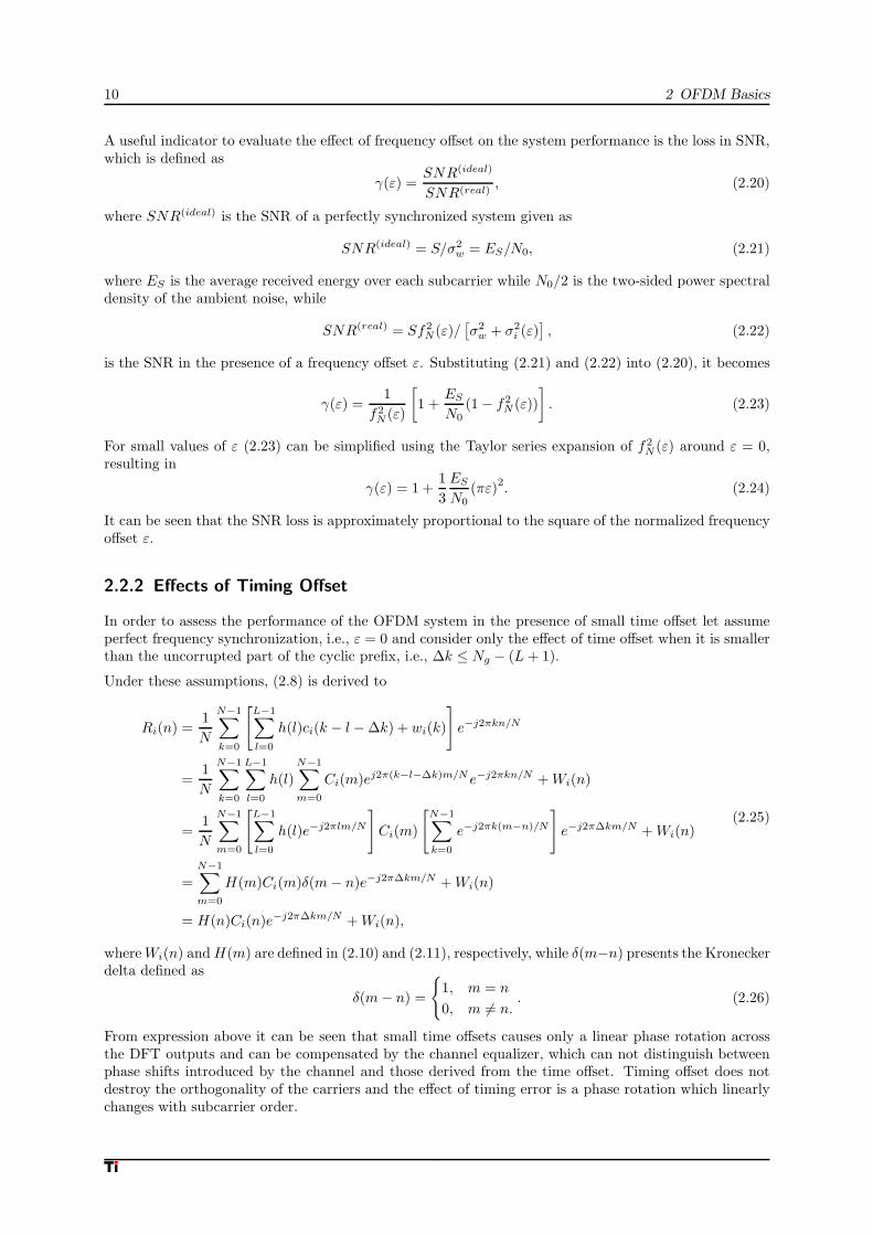
2.2.2 Effects of Timing Offset

In order to assess the performance of the OFDM system in the presence of small time offset let assumeperfect frequency synchronization, i.e., ε = 0 and consider only the effect of time offset when it is smallerthan the uncorrupted part of the cyclic prefix, i.e., ∆k ≤ Ng − (L + 1).

Under these assumptions, (2.8) is derived to

Ri(n) =1

N

N−1∑

k=0

[

L−1∑

l=0

h(l)ci(k − l − ∆k) + wi(k)

]

e−j2πkn/N

=1

N

N−1∑

k=0

L−1∑

l=0

h(l)

N−1∑

m=0

Ci(m)ej2π(k−l−∆k)m/N e−j2πkn/N + Wi(n)

=1

N

N−1∑

m=0

[

L−1∑

l=0

h(l)e−j2πlm/N

]

Ci(m)

[

N−1∑

k=0

e−j2πk(m−n)/N

]

e−j2π∆km/N + Wi(n)

=N−1∑

m=0

H(m)Ci(m)δ(m − n)e−j2π∆km/N + Wi(n)

= H(n)Ci(n)e−j2π∆km/N + Wi(n),

(2.25)

where Wi(n) and H(m) are defined in (2.10) and (2.11), respectively, while δ(m−n) presents the Kroneckerdelta defined as

δ(m − n) =

{

1, m = n

0, m 6= n.. (2.26)

From expression above it can be seen that small time offsets causes only a linear phase rotation acrossthe DFT outputs and can be compensated by the channel equalizer, which can not distinguish betweenphase shifts introduced by the channel and those derived from the time offset. Timing offset does notdestroy the orthogonality of the carriers and the effect of timing error is a phase rotation which linearlychanges with subcarrier order.


2.2.3 Equalization

Channel equalization is the process through which a coherent receiver compensates for any distortioninduced by frequency-selective fading. For the sake of simplicity, ideal timing and frequency synchro-nization is considered throughout this subsection. The channel is assumed static over each OFDM block,but can vary from block to block. Under these assumptions, and assuming that the receiver is perfectlysynchronized, i.e, ε = 0 and ∆k = 0, the output of the receiver’s DFT unit during the ith symbol is givenby

Ri(n) = Hi(n)Ci(n) + Wi(n), 0 ≤ n ≤ N − 1 (2.27)

where Ci(n) is the complex data symbol and Wi(n) as well as H(m) are defined in (2.10) and (2.11),respectively. An important feature of OFDM is that channel equalization can independently be performedover each subcarrier by means of a bank of one-tap multipliers. As shown in Fig. 2.5, the nth DFT outputRi(n) is weighted by a complex-valued coefficient Pi(n) in order to compensate for the channel-inducedattenuation and phase rotation. The equalized sample Yi(n) = Pi(n)Ri(n) is then subsequently passed tothe detection unit, which delivers final decisions Ci(n) on the transmitted data. Intuitively, the simplest

channelequalization

decisiondevice

Ri(n) Yi(n) Ci(n)

Pi(n)

Figure 2.5: Block diagram of an OFDM receiver

method for the design of the equalizer coefficients, is to perform a pure channel inversion, know asZero-Forcing (ZF) criterion. The equalizer coefficients are then given by

Pi(n) =1

Hi(n), (2.28)

while the DFT output takes the form

Yi(n) =Ri(n)

Hi(n)= Ci(n) +

Wi(n)

Hi(n), 0 ≤ n ≤ N − 1. (2.29)

From (2.29) it can be noticed that ZF equalization is capable of totally compensating for any distortioninduced by the wireless channel. However, the noise power at the equalizer output is given by σ2

w/|Hi(n)|2and may be excessively large over deeply faded subcarriers characterized by low channel gains.

Inherent system requirement for ZF equalizer is the knowledge of the channel transfer function Hi(n).Therefore, in many wireless OFDM systems, sequence of data symbols is preceded by several referenceOFDM symbols (preambles) known to the receiver, forming the OFDM frame. Typical frame structureis shown in Fig. 2.6 where preambles are typically used for synchronization and/or channel estimationpurposes. In typical fixed wireless standards as WLAN, it can be assumed that the channel remains staticover frame duration, i.e., Hi(n) = H(n) for i = 1, . . . , I, where I is the total number of OFDM symbolswithin one frame. Then, channel estimates obtained from the preambles can be used to coherently detectthe entire payload.

Assuming that the OFDM frame has one preamble with index i = p = 1, the output of the DFT block(2.27) can be written as

Rp(n) = H(n)Cp(n) + Wp(n), 0 ≤ n ≤ N − 1 (2.30)

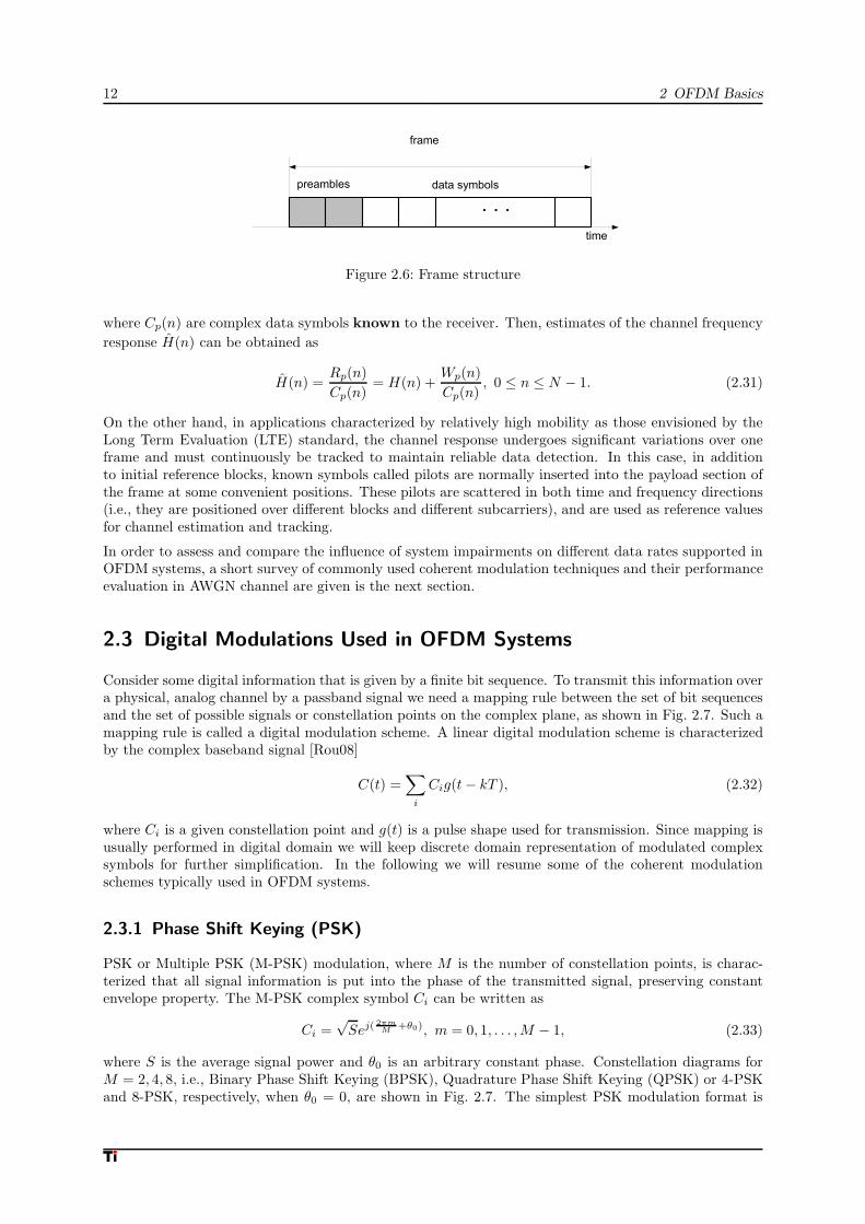
12 2 OFDM Basics

Figure 2.6: Frame structure

where Cp(n) are complex data symbols known to the receiver. Then, estimates of the channel frequency

response H(n) can be obtained as

H(n) =Rp(n)

Cp(n)= H(n) +

Wp(n)

Cp(n), 0 ≤ n ≤ N − 1. (2.31)

On the other hand, in applications characterized by relatively high mobility as those envisioned by theLong Term Evaluation (LTE) standard, the channel response undergoes significant variations over oneframe and must continuously be tracked to maintain reliable data detection. In this case, in additionto initial reference blocks, known symbols called pilots are normally inserted into the payload section ofthe frame at some convenient positions. These pilots are scattered in both time and frequency directions(i.e., they are positioned over different blocks and different subcarriers), and are used as reference valuesfor channel estimation and tracking.

In order to assess and compare the influence of system impairments on different data rates supported inOFDM systems, a short survey of commonly used coherent modulation techniques and their performanceevaluation in AWGN channel are given is the next section.

2.3 Digital Modulations Used in OFDM Systems

Consider some digital information that is given by a finite bit sequence. To transmit this information overa physical, analog channel by a passband signal we need a mapping rule between the set of bit sequencesand the set of possible signals or constellation points on the complex plane, as shown in Fig. 2.7. Such amapping rule is called a digital modulation scheme. A linear digital modulation scheme is characterizedby the complex baseband signal [Rou08]

C(t) =∑

i

Cig(t − kT ), (2.32)

where Ci is a given constellation point and g(t) is a pulse shape used for transmission. Since mapping isusually performed in digital domain we will keep discrete domain representation of modulated complexsymbols for further simplification. In the following we will resume some of the coherent modulationschemes typically used in OFDM systems.

2.3.1 Phase Shift Keying (PSK)

PSK or Multiple PSK (M-PSK) modulation, where M is the number of constellation points, is charac-terized that all signal information is put into the phase of the transmitted signal, preserving constantenvelope property. The M-PSK complex symbol Ci can be written as

Ci =√

Sej( 2πmM +θ0), m = 0, 1, . . . , M − 1, (2.33)

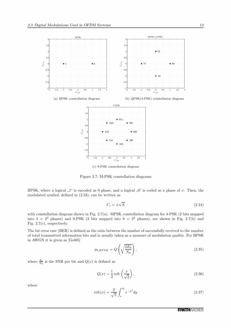
where S is the average signal power and θ0 is an arbitrary constant phase. Constellation diagrams forM = 2, 4, 8, i.e., Binary Phase Shift Keying (BPSK), Quadrature Phase Shift Keying (QPSK) or 4-PSKand 8-PSK, respectively, when θ0 = 0, are shown in Fig. 2.7. The simplest PSK modulation format is

2.3 Digital Modulations Used in OFDM Systems 13

−2 −1.5 −1 −0.5 0 0.5 1 1.5 2−2

−1.5

−1

−0.5

0

0.5

1

1.5

2

Ci,Re

Ci,

Im

BPSK

1 0

(a) BPSK constellation diagram

−2 −1.5 −1 −0.5 0 0.5 1 1.5 2−2

−1.5

−1

−0.5

0

0.5

1

1.5

2

Ci,Re

Ci,

Im

QPSK (4-PSK)

10

01

0011

(b) QPSK(4-PSK) constellation diagram

−2 −1.5 −1 −0.5 0 0.5 1 1.5 2−2

−1.5

−1

−0.5

0

0.5

1

1.5

2

Ci,Re

Ci,

Im

8-PSK

000

101

111

110

010

100

001

011

(c) 8-PSK constellation diagram

Figure 2.7: M-PSK constellation diagrams

BPSK, where a logical”1“ is encoded as 0 phase, and a logical

”0“ is coded as a phase of π. Then, the

modulated symbol, defined in (2.33), can be written as

Ci = ±√

S (2.34)

with constellation diagram shown in Fig. 2.7(a). MPSK constellation diagram for 4-PSK (2 bits mappedinto 4 = 22 phases) and 8-PSK (3 bits mapped into 8 = 23 phases), are shown in Fig. 2.7(b) andFig. 2.7(c), respectively.

The bit error rate (BER) is defined as the ratio between the number of successfully received to the numberof total transmitted information bits and is usually taken as a measure of modulation quality. For BPSKin AWGN it is given as [Gol05]

pb,BPSK = Q

(

√

2Eb

N0

)

, (2.35)

where Eb

N0is the SNR per bit and Q(x) is defined as

Q(x) =1

2erfc

(

x√2

)

, (2.36)

where

erfc(x) =2√π

∫ ∞

x

e−y2

dy (2.37)

14 2 OFDM Basics

is the complementary error function (erfc). For higher order M-PSK, where M > 4, the symbol errorrate (SER) can be expressed as

ps,M−PSK = 2Q

(

√

2Eb log2 M

N0sin

π

M

)

, (2.38)

where Es

N0= Eb log2 M

N0is the SNR per symbol. For Gray-coded modulations, i.e., when adjacent constel-

lation points differ in one bit as in Fig. 2.7, the BER in the high SNR regime for each modulation isapproximately

pb,M−PSK ≈ ps,M−PSK

log2 M.

2.3.2 Quadrature Amplitude Modulation (QAM)

−2 −1.5 −1 −0.5 0 0.5 1 1.5 2−2

−1.5

−1

−0.5

0

0.5

1

1.5

2

Ci,Re

C i,I

m

4-QAM

(a) 4-QAM constellation diagram

−2 −1.5 −1 −0.5 0 0.5 1 1.5 2−2

−1.5

−1

−0.5

0

0.5

1

1.5

2

Ci,Re

C i,I

m

16-QAM

(b) 16-QAM constellation diagram

−2 −1.5 −1 −0.5 0 0.5 1 1.5 2−2

−1.5

−1

−0.5

0

0.5

1

1.5

2

Ci,Re

C i,I

m

64-QAM

(c) 64-QAM constellation diagram

−2 −1.5 −1 −0.5 0 0.5 1 1.5 2−2

−1.5

−1

−0.5

0

0.5

1

1.5

2

Ci,Re

C i,I

m

256-QAM

(d) 256-QAM constellation diagram

Figure 2.8: QAM constellation diagrams

QAM is a bandwidth efficient signaling scheme that, unlike M-PSK does not possess a constant envelopeproperty, thus offering higher bandwidth efficiency, i.e., more bits per second (bps) can be transmittedin a given frequency bandwidth. QAM modulated signals for M constellation points can be written as

Ci =√

SK(Xi + jYi),

where Xi, Yi ∈{

±1,±3, . . . ,√

M − 1}

and K is a scaling factor for normalizing the average power for

all constellations to S. The K value for various constellations is shown in Table 2.1. CorrespondingQAM constellation diagrams for 4-QAM (2 bits mapped into 4 = 22 points), 16-QAM (4 bits mappedinto 16 = 24 points), 64-QAM (6 bits mapped into 64 = 26 points), and 256-QAM (8 bits mapped into

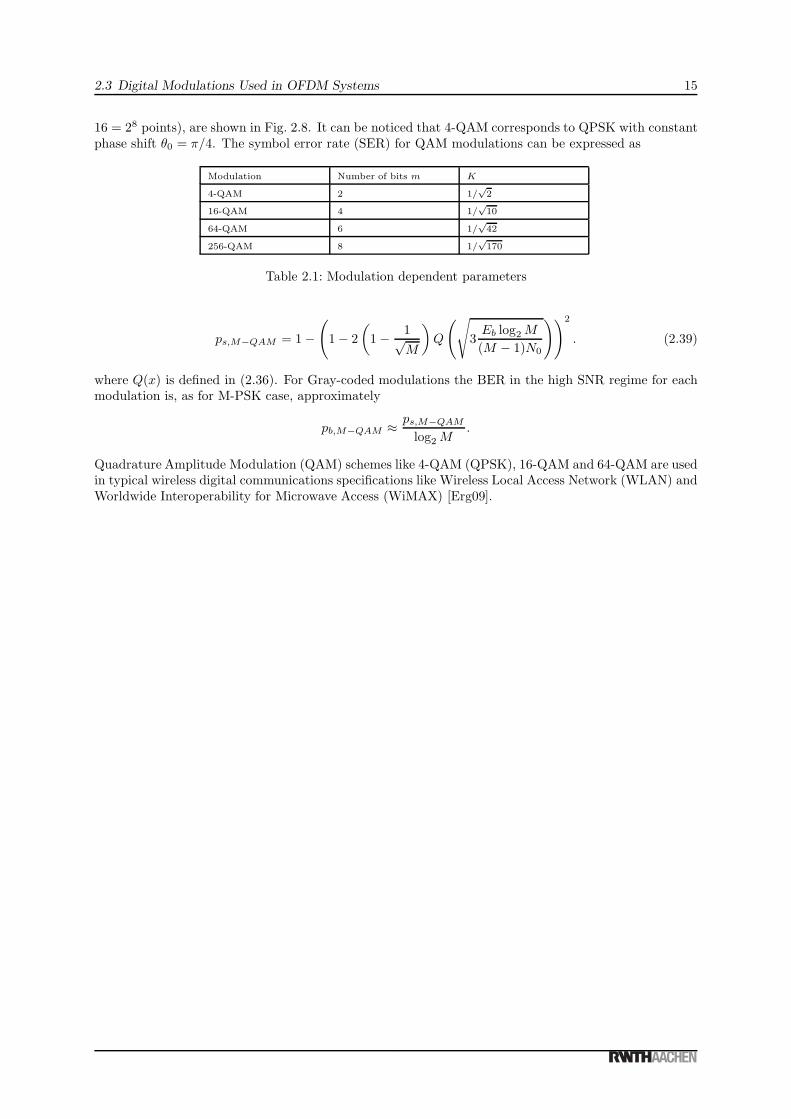
2.3 Digital Modulations Used in OFDM Systems 15

16 = 28 points), are shown in Fig. 2.8. It can be noticed that 4-QAM corresponds to QPSK with constantphase shift θ0 = π/4. The symbol error rate (SER) for QAM modulations can be expressed as

Modulation Number of bits m K

4-QAM 2 1/√

2

16-QAM 4 1/√

10

64-QAM 6 1/√

42

256-QAM 8 1/√

170

Table 2.1: Modulation dependent parameters

ps,M−QAM = 1 −(

1 − 2

(

1 − 1√M

)

Q

(√

3Eb log2 M

(M − 1)N0

))2

. (2.39)

where Q(x) is defined in (2.36). For Gray-coded modulations the BER in the high SNR regime for eachmodulation is, as for M-PSK case, approximately

pb,M−QAM ≈ ps,M−QAM

log2 M.

Quadrature Amplitude Modulation (QAM) schemes like 4-QAM (QPSK), 16-QAM and 64-QAM are usedin typical wireless digital communications specifications like Wireless Local Access Network (WLAN) andWorldwide Interoperability for Microwave Access (WiMAX) [Erg09].

16 2 OFDM Basics

3 Software Defined Radio and GNU RadioFramework

In this chapter a general introduction to the SDR concept is given. Additionally, advantages of SDRsand given hardware limitations are addressed. Here, the GNU Radio SDR framework is presented givinginsight into the basic architectural features.

A SDR is a radio that is built entirely or in large parts in software, which runs on a general purposecomputer. A more extensive definition is given by Joseph Mitola, who established the term SoftwareRadio [Mit06]:

”A software radio is a radio whose channel modulation waveforms are defined in software. That is,

waveforms are generated as sampled digital signals, converted from digital to analog via a wideband digital-to-analog converter (DAC) and then possibly upconverted from intermediate frequency (IF) to RF. Thereceiver, similarly, employs a wideband ADC that captures all of the channels of the software radio node.The receiver then extracts, downconverts and demodulates the channel waveform using software on ageneral purpose processor. Software radios employ a combination of techniques that include multi-bandantennas and RF conversion; wideband ADC and DAC; and the implementation of IF, baseband andbitstream processing functions in general purpose programmable processors. The resulting software definedradio (or

”software radio“) in part extends the evolution of programmable hardware, increasing flexibility

via increased programmability.“

This means, that instead of using analog circuits or a specialized Digital Signal Processor (DSP) toprocess radio signals, the digitized signals are processed by architecture independent, and high levelsoftware running on general purpose processors. The term radio designates any device, that transmitsand/or receives radio waves. While most modern radios contain firmware that is written in some kind ofprogramming language, the important distinction in a software radio is that it is not tailored to a specificchip or platform, and it is therefore possible to reuse its code across different underlying architectures[Mue08].

3.1 Ideal Software Defined Radio and Practical Limitations

In the ideal case, the only hardware that is needed besides a computer is an antenna and an ADC for thereceiver, as well as a digital-to-analog converter (DAC) for the transmitter. A SDR would thus look asdepicted in Fig. 3.1. In the receiver, a transmitted radio signal is picked up by an antenna, and then fedinto an ADC to sample it. Once digitized, the signal is sent to some general purpose computer (e.g. anembedded PC) for processing. The transmitter looks very similar, except that the signal is sent in thereverse direction, and a DAC is used instead of an ADC. In a complete transceiver, the processing unitand the antenna may be shared between receiver and transceiver.

While the approach presented in the previous section is very simple and (in the ideal case) extremelyversatile, it is not practical, due to limitations in real hardware. However, various solutions have beensuggested to overcome these problems. A quick look at the different hardware limitations is given below.For better readability, only the receiving side is discussed. The transmitting side is symmetrical.

• Analog-Digital Converters : According to sampling theorem, the sampling rate of ADC must be atleast twice as high as the bandwidth of received signal which limits the maximum bandwidth of thereceived signal. Current ADCs are capable of sampling rates in the area of 100 Mega Samples PerSecond (MSPS), which translates to a bandwidth of 50 MHz. While this bandwidth is enough formost current applications, the carrier frequency is usually higher than 50 MHz. In practice, a RF

18 3 Software Defined Radio and GNU Radio Framework

PC PCADCDAC

Figure 3.1: Ideal SDR transmission

frontend is therefore usually required, to convert the received signal to an intermediate frequency(IF).

The second parameter, the ADC resolution influences the dynamic range of the receiver. As eachadditional bit doubles the resolution of the sampled input voltage, the dynamic range can be roughlyestimated as R = 6dB × n where R is the dynamic range and n the number of bits in the ADC.As ADCs used for SDR usually have a resolution of less than 16 bits, it is important to filter outstrong interfering signals, such as signals from mobile phones, before the wideband ADC. This isusually done in the RF frontend.

• Bus Speed : Another problem lies in getting the data from the ADC to the computer. For anypractical bus, there is a maximum for the possible data rate, limiting the product of sample rateand resolution of the samples. The speed of common buses in commodity PCs ranges from a fewMbps to several Gbps as an example, the Peripheral Component Interconnect (PCI) 2.2 bus has atheoretical maximum speed of 4256 Mbps.

• Performance of the Processing Unit : For real-time processing, the performance of the CentralProcessing Unit (CPU)and the sample rate limit the number of mathematical operations that canbe performed per sample, as samples must be processed as fast as they arrive. In practice, thismeans that fast CPUs, clever programming and possibly parallelization is needed. If this does notsuffice, a compromise must be found, to use a less optimal but faster signal processing algorithm.

• Latency: Since general purpose computers are not designed for real-time applications, a rather highlatency can occur in practical SDRs. While latency is not much of an issue in transmit-only orreceive-only applications, many wireless standards, such as Global System for Mobile communi-cations (GSM) or Wireless Metropolitan Access Network (DECT) require precise timing, and aretherefore very difficult to implement in an SDR.

Because of the use of general purpose processing units, an implementation of a given wireless applicationas an SDR is likely to use more power and occupy more space than a hardware radio with analog filteringand possibly a dedicated signal processor. Because an SDR contains more complex components than ahardware radio, it will likely be more expensive, given a large enough production volume.

Nevertheless, SDR concepts carry the flexibility of software over to the radio world and introduces anumber of interesting possibilities. For example, very much the same way as someone may load a wordprocessor or an Internet browser on a PC, depending on the task at hand, a SDR could allow its userto load a different configuration, depending on whether the user wants to listen to a broadcast radiotransmission, place a phone call or determine the position via Global Positioning System (GPS). A newapplication may even be added after the device is finished. Since the same hardware can be used forany application, a great reuse of resources is possible. Another interesting possibility enabled by SDRis the creation of a cognitive radio, which is aware of its RF environment and adapts itself to changesin the environment. By doing this, a cognitive radio can use both the RF spectrum and its own energyresources more efficiently. As a cognitive radio requires a very high degree of flexibility, the concept ofSDR is very convenient for its practical realization.

3.2 GNU Radio Architecture

GNU Radio is an open source, free software toolkit for building SDRs [GNUac]. It is designed to runon personal computers and (PC) combined with minimal hardware allowing the construction of simple

3.2 GNU Radio Architecture 19

software radios [Mue08]. The project was started in early 2000 by Eric Blossom and has evolved intoa mature software infrastructure that is used by a large community of developers. It is licensed underthe GNU General Public License (GPL), thus anyone is allowed to use, copy and modify GNU Radiowithout limits, provided that extensions are made available under the same license. While GNU Radiowas initially started on a Linux platform, it now supports various Windows, MAC and various Unixplatforms.

GNU Radio architecture consists of two components. The first component is the set of numerous buildingblocks which represents C++ implementations of digital signal processing routines such as (de)modulation,filtering, (de)coding and I/O operations such as file access. For further information about C++ program-ming see for example [Mey98, Mey99, Mey01, Str00, SA07]. The second component is a framework tocontrol the data flow among blocks, implemented as Python scripts enabling easy reconfiguration andcontrol of various system functionalities and parameters. For further studies on Python see e.g. [Mar03].By

”wiring“ together such building blocks, a user can create a software defined radio, similar to connecting

physical RF building blocks to create a hardware radio. An RF interface for GNU Radio architectureis realized by USRP boards, a general purpose RF hardware, which performs computationally intensiveoperations as filtering, up- and down-conversion. The USRP and its recent version USRP2 are connectedto PC over a USB 2.0 and Ethernet cable, respectively, and are controlled through a robust applicationprogramming interface (API) provided by GNU Radio.

3.2.1 Gnu Radio Framework

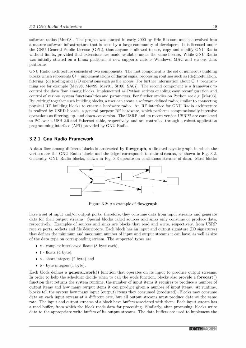
A data flow among different blocks is abstracted by flowgraph, a directed acyclic graph in which thevertices are the GNU Radio blocks and the edges corresponds to data streams, as shown in Fig. 3.2.Generally, GNU Radio blocks, shown in Fig. 3.3 operate on continuous streams of data. Most blocks

Figure 3.2: An example of flowgraph

have a set of input and/or output ports, therefore, they consume data from input streams and generatedata for their output streams. Special blocks called sources and sinks only consume or produce data,respectively. Examples of sources and sinks are blocks that read and write, respectively, from USRPreceive ports, sockets and file descriptors. Each block has an input and output signature (IO signatures)that defines the minimum and maximum number of input and output streams it can have, as well as sizeof the data type on corresponding stream. The supported types are

• c - complex interleaved floats (8 byte each),

• f - floats (4 byte),

• s - short integers (2 byte) and

• b - byte integers (1 byte).

Each block defines a general work() function that operates on its input to produce output streams.In order to help the scheduler decide when to call the work function, blocks also provide a forecast()function that returns the system runtime, the number of input items it requires to produce a number ofoutput items and how many output items it can produce given a number of input items. At runtime,blocks tell the system how many input (output) items they consumed (produced). Blocks may consumedata on each input stream at a different rate, but all output streams must produce data at the samerate. The input and output streams of a block have buffers associated with them. Each input stream hasa read buffer, from which the block reads data for processing. Similarly, after processing, blocks writedata to the appropriate write buffers of its output streams. The data buffers are used to implement the


GNU RadioBlock

GNU RadioBlock

C++ class

Figure 3.3: GNU Radio blocks

edges in the flowgraph: the input buffers for a block are the output buffers of the upstream block inthe flowgraph. GNU Radio buffers are single writer, multiple reader FIFO (First in First Out) buffers.Several blocks are connected in Python forming a flowgraph using the connect function which specifies

Hierarchical block

Sink

Source

DSP

Sink

Figure 3.4: An example of a flowgraph with a hierarchical block

how the output stream(s) of a processing block connects to the input stream of one or more downstreamblocks. The flowgraph mechanism then automatically builds the flowgraph; the details of this processare hidden from the user. A key function during flowgraph construction is the allocation of data buffersto connect neighboring blocks. The buffer allocation algorithm considers the input and output blocksizes used by blocks and the relative rate at which blocks consume and produce items on their input andoutput streams. Once buffers have been allocated, they are connected with the input and output streamsof the appropriate block.

Several blocks can also be combined in a new block, named hierarchical block, as shown in Fig. 3.4.Hierarchical blocks are implemented in Python and together with other blocks can be combined intonew hierarchical blocks. Input and output ports of hierarchical blocks have same constraints as thoseof terminal blocks.

The GNU Radio scheduler executes the graph that was built by the flowgraph mechanism. During theexecution, the scheduler queries each block for its input requirements and it uses the above-mentionedforecast functions to determine how much data the block can consume from its available input. If sufficientdata is available in the input buffers, the schedule calls the block’s work function. If a block does nothave sufficient input, the scheduler simply moves on to the next block in the graph. Skipped blocks willbe executed later, when more input data is available. The scheduler is designed to operate on continuousdata streams.

in FIR

NCO

Mult outAdd

Noise

Figure 3.5: Wireless communication channel simulation model

3.2 GNU Radio Architecture 21

3.2.2 An Example: Wireless Channel Simulation

It will be shown how a model for a static wireless channel can be implemented as a GNU Radio hier-archical block. The channel is affected by multipath propagation, frequency offset and additive noise.Fig. 3.5 shows a model with internal blocks and corresponding ports [Aur09].

Multipath effects are modeled using a FIR-filter where complex filter coefficients are taken from anarbitrary channel model, e.g. Rayleigh channel model. The signal from an input port is derived to thecorresponding GNU Radio block gr.fir filter ccc. The suffix ccc denotes that the input stream, outputstream and filter coefficients are of complex data types.

According to (2.4), the frequency offset is modeled as a sinus wave with fixed frequency and is multipliedwith the incoming signal. The corresponding GNU radio blocks are the complex sine signal sourcegr.sig source c and the multiplicator with complex inputs and outputs gr.multiply cc, respectively.

Finally, complex additive Gaussian noise generated by gr.noise source c is added to the incoming signalin the gr.add cc block and the result is directed to the output port.

The initial parameters of a given hierarchical block, named simple channel, are additive noise standardvariance, frequency offset normalized to sampling frequency and complex FIR-filter coefficients. IOsignatures of input and output ports are identical and in the framework there is minimum one port andmaximum one port for both input and output.

During runtime, internal blocks are initialized and connected to the flowgraph. The corresponding pythonscript is shown below.

Program 1 Python script for simulation of a wireless communication channel

class simple_channel(gr.hier_block2):

def __init__(self, noise_rms, frequency_offset, channel_coefficients):

gr.hier_block2.__init__(self, "simple_channel", # Blocktype Identifier

gr.io_signature(1,1,gr.sizeof_gr_complex), # incoming

gr.io_signature(1,1,gr.sizeof_gr_complex)) # outgoing

# for example channel_coefficients = [0.5+0.1j, 0.2-0.01j]

multipath_sim = gr.fir_filter_ccc(1, channel_coefficients)

# frequency_offset normalized to sampling frequency

# amplitude = 1.0, DC offset = 0.0

offset_src = gr.sig_source_c(1, gr.GR_SIN_WAVE, frequency_offset, 1.0, 0.0)

mix = gr.multiply_cc()

# noise_rms -> var(noise) = noise_rms**2

noise_src = gr.noise_source_c(gr.GR_GAUSSIAN, noise_rms/sqrt(2))

add_noise = gr.add_cc()

# describe signal paths

self.connect(self, multipath_sim) # incoming port

self.connect(multipath_sim, (mix,0))

self.connect(offset_src, (mix,1))

self.connect(mix, (noise_add,0))

self.connect(noise_src, (noise_add,1))

self.connect(noise_add, self) # outgoing port

4 GNU Radio OFDM TransceiverImplementation

This chapter gives an introduction to an SDR based GNU Radio OFDM transceiver implemented in ourinstitute [ZAM09]. A system diagram of our OFDM framework is shown in Fig. 4.1. Transmitter and

��

��

��

��

��

��

��

��

��

��

CORBA consumer CORBA supplier

Demapper BER, CSI, SNRestimates

CORBA supplier CORBA consumer

Static Tx Mapper

Rx USRPTx USRP

Rx nodeTx node

QoS (BER)requirement

Resource

manager

parameters (variable rate/power) (variable rate/power)

Tx/Rx GUI

Wireless link

Event Channel

Figure 4.1: The system overview

receiver node are composed of a host commodity computer and general purpose RF hardware, USRP.The baseband signal processing at the host computers is implemented in the GNU Radio framework.Within the framework, additional OFDM specific GNU Radio blocks are implemented, particularly atreceiver’s synchronization stage, since OFDM systems are highly sensitive to time offsets and oscillators’mismatch between transmitter and receiver due to necessity for subchannel orthogonality, see Section 2.2.The main adaptive and capacity achieving functionality is performed in blocks for adaptive mapping anddemapping of various rates (taken from the set of available modulations given in Table 4.1) and powerlevels across subchannels.

Algorithms for estimation of link quality, expressed through average SNR and channel state information(CSI) over subchannels, are extensively studied and implemented at the receiver. Furthermore, in orderto assess system performance, the receiver implementation contains blocks for BER measurements.

The communication between transmitter and receiver node is organized as a reconfigurable continuousone-way transmission of OFDM symbol frames. As shown in Table 4.1, the set of input configurationparameters can be divided into two classes. The set of static parameters containing FFT, number ofsubchannels, frame size, etc., is initialized at transmission start and is known to both nodes. The set ofdynamic parameters which are reconfigurable at runtime includes total transmit power and allocatedrate and power over subchannels.

The backbone of the system is realized over a local Ethernet network by a Common Object RequestBroker Architecture (CORBA) event service [GNUrg], a distributed communication model that allowsan application to send an event that will be received by any number of objects located in different logicaland/or physical entities. For more information on CORBA see [MR97, OHE97]. Estimated parametersthat indicate link quality (average SNR, CSI, and BER) and current static transmitter’s parameters are

24 4 GNU Radio OFDM Transceiver Implementation

(a) The transmitter’s GUI (b) The receiver’s GUI with interactive control interface

Figure 4.2: The framework’s GUI with interactive control interface

supplied as CORBA events to the event channel which allows other components (consumers) withinthe system to register their interests in events. The central control unit that determines optimal inputtransmission parameters for given requirements is called resource manager. Controlled by an interactivegraphical user interface (GUI) it consumes supplied events forwarded from the event channel, performsallocation in an optimal manner, and supplies new transmission parameters, i.e., total transmit powerand power/rate per subchannel, which are finally consumed by other components in the system. The

Carrier frequency (static) 2400 − 2483 MHzBandwidth (static) Variable, up to 2 MHzFFT length (static) 64 − 1024Frame length (static) VariableModulations (dynamic) BPSK, QPSK, 8-PSK, 16-QAM, 32-QAM,

64-QAM, 128-QAM, 256-QAMPower (dynamic) Up to 20 mW

Table 4.1: OFDM symbol parameters

GUI, facilitating the demonstration, is developed in Qt/C++ framework. The transmitter’s GUI containsstatic transmission parameters and current allocation of rate and power over subchannels, as shown inFig. 4.2(a). Furthermore, the receiver’s GUI, given in Fig. 4.2(b), dynamically shows estimated channelparameters (average SNR, CSI, BER) and contains an interactive interface for controlling allocationstrategies and transmission parameters in the resource manager.

The system can also run in simulation mode on a single PC, without the RF interface (USRP boards),where transmitter and receiver

”communicate“ over an artificial channel. A set of channel models available

through IT++ libraries [GNUpp] is ported to GNU Radio framework in order to evaluate the systemperformance excluding hardware impairments.

Due to the high modularity and distributed nature of the system supported by a generalized interface,the dedicated resource manager can be easily reconfigured for different classes of given requirementsand various sets of controllable parameters.

5 Preparatory Exercises

5.1 Exercise: System Performance in an AWGN Channel

Note: For this exercise SNR values are given in decibel (dB). The relation to the linear value is given by

SNR[dB] = 10 · log10(SNR). (5.1)

1. Determine the missing BER entries pb in Table 5.1 for given values of received SNR and variousmodulation schemes using (2.35) and (2.39).Hints: For calculating the missing entries of Table 5.1 use the erfc function which is a member ofthe standard Matlab library. Calculated values should be rounded to two digits, e.g., if the calculatedvalue is 0.001234 write it as 1.23 · 10−3.

Table 5.1: BER pb to SNR [dB] dependencies for various modulation schemes

ES/N0 [dB] 0 5 10 15 20 25 30

BERBP SK

BER4−QAM

BER16−QAM

BER64−QAM

BER256−QAM

2. Draw graphs for the BER pb depending on the SNR ES/N0 into Fig. 5.1. Sketch the graphs forall modulation schemes given in Table 5.1 using all entries from this table. Give an appropriatelegend.

0 5 10 15 20 25 3010

−4

10−3

10−2

10−1

100

ES/N

0 [dB]

p b

Figure 5.1: The BER over SNR performance for various modulation schemes

26 5 Preparatory Exercises

3. Using the results from Fig. 5.1, determine the required SNR ES/N0 values for achieving a BERof 10−3. What are the differences of the determined SNRs for BPSK, 16-QAM, and 256-QAM?

5.2 Exercise: SNR Loss due to Frequency Offset

1. Determine the missing SNR loss entries and fill in the Table 5.2 for different frequency offsets andSNRs using (2.23).Notes: Calculate SNR losses in decibel (dB). The relation to the linear value is given by

γ(ε)[dB] = 10 · log10(γ(ε)). (5.2)

Assume that π εN is small.

Table 5.2: SNR losses for different values of frequency offsets and SNRs

ε 10−2 2 · 10−2 5 · 10−2 10−1 2 · 10−1 4 · 10−1

γ(ε)|ES/N0=5[dB][dB]




2. Draw curves for the SNR loss γ(ε) in dependency of the frequency offset ε into Fig. 5.2. Draw thegraphs to all SNRs given in Table 5.2 taking all entries from this table. Give an appropriate legend.

10−2

10−1

0

1

2

3

4

5

6

7

8

ε

γ(ε)

[dB

]

Figure 5.2: SNR loss over frequency offsets for different SNRs

3. Using the results from Fig. 5.2, determine the maximum tolerable frequency offsets ε for preservinga SNR loss below 1 [dB].

4. Using (2.5), for system bandwidth of 1TS

= 2 MHz and DFT length of N = 256, calculate themaximum tolerable frequency offset fd in Hz for preserving the same SNR losses as in 3.

5.2 Exercise: SNR Loss due to Frequency Offset 27

5. For the same value of frequency offset fd in Hz as in 4., what is the SNR loss for 1TS

= 5 MHz andN = 256?

6. For the same value of frequency offset fd in Hz as in 4., what is the SNR loss for 1TS

= 2 MHz andN = 64?

7. Describe the observed influence of signal bandwidth as well as the DFT length on the SNR loss.

28 5 Preparatory Exercises

6 Laboratory Exercises

6.1 Description

The goal of these lab exercises is to evaluate the system performance of a given SDR framework in real-time transmission conditions and compare them with previously obtained analytical results. The highflexibility of the developed framework allows for high reconfigurability of transmission signal parametersand easy monitoring of the desired performance.

During the exercises there will be up to 5 groups of 2-3 students working with 2 PCs equipped with USRPs.Exercises 6.2.1, 6.3 and 6.4.1 should be done on a single PC and each group should be appropriatelydivided. For exercises 6.2.2 and 6.4.2 the whole group should use 2 PCs in order to perform real-timetransmission.

Before beginning to work on the following exercises you need to start CORBA’s nameand event service and set appropriate configurations as it is described in tasks 1-8 in Ap-pendix A.2.

6.2 Lab 1: AWGN Channel

Firstly, the analytical results obtained in the preparatory exercises of Section 5.1 will be verified inlocal environment by means of a simulated AWGN channel. Afterwards, the system performance in areal-time transmission with USRP boards will be evaluated and compared to the analytical results.

6.2.1 Local Environment

This task needs to be performed on a single PC. Given an AWGN simulation model as shown in Fig. 6.1transmitter and receiver communicate over the channel which is realized using a FIFO pipe file.

Add

Noise

Tx Rx

Figure 6.1: AWGN channel model

1. Open six terminal windows which will be used for system’s manipulation.

2. In the first and the second terminal start the transmitter and the receiver, respectively, working inlocal environment for particular SNR values given in Table 6.1 by executing following scripts inseparate terminal windows:./usrp_tx --to-file ~/omnilog/channel --bandwidth=1M --fft-length=256 --subcarriers=200

--station-id=100 --nameservice-ip=your comp --awgn --snr=snr valueand./usrp_rx --from-file ~/omnilog/channel --bandwidth=1M --fft-length=256 --subcarriers=200

--station-id=1 --nameservice-ip=your comp --scatterplot

where your comp denotes the operating PC hostname and snr value is the simulated SNR value.

30 6 Laboratory Exercises

3. • To set the transmit amplitude for obtaining the desired SNR, in the third terminal start thecalibration resource manager by executing:./run_script ../python/rm_calibrate.py

• In order to monitor the system performance start the transmitter’s and the receiver’s GUIs inthe fourth and the fifth terminal, respectively, as it is described in Appendix A.3.

• At the receiver’s GUI, fit the values of estimated SNR to the values given in Table 6.1 bychanging transmission amplitude (changing the values in textfield Constraint). The selectedtransmission amplitude will be used further on for actual simulations.

• Stop the calibration script in the third terminal.

4. Start the appropriate resource manager in the third terminal by executing:./run_script ../python/rm_exercise_1_1.py -a tx amplitude --snr=snr valuewhere snr value denotes the nominal SNR value given in Table 6.1 and tx amplitude is thepreviously calibrated transmission amplitude.

5. In the sixth terminal start the constellation diagrams as it is described in Appendix A.3.

6. During simulation, read measured SNR and BER from the resource manager terminal or from thelog file located in ˜/omnilog/ and fill in the Table 6.1. When measurement is over stop the resourcemanager in the third terminal.

7. Repeat the steps 2, 4-6 for all SNR values given in Table 6.1.

Table 6.1: The BER for various measured SNRs and modulation schemes in local environment

Nominal Es/N0 [dB] 5 10 15 20 25 30

Measured Es/N0 [dB]

BERBPSK

Measured Es/N0 [dB]

BER4−QAM

Measured Es/N0 [dB]

BER16−QAM

Measured Es/N0 [dB]

BER64−QAM

Measured Es/N0 [dB]

BER256−QAM

8. Add the BER curves from Table 6.1 to Fig. 5.1 and complete the legend.

9. Compare the obtained curves.

6.2.2 Real-time Transmission

This task needs to be performed on two PCs. For real-time transmission in realistic channel conditionsthe channel and AWGN blocks shown in Fig. 6.1 are replaced by the real channel between two USRPboards.

1. On the transmitter’s PC in the first terminal start the transmitter by executing:./usrp_tx -f frequency --bandwidth=1M --fft-length=256

--subcarriers=200 --station-id=100 --nameservice-ip=comp 1where comp 1 is the name of the transmitting PC while transmission frequency depends on thedaughterboard type of your USRP. It will be given to you by the supervisors.

2. In order to use the same name service which runs on a transmitter’s PC, on a receiver’s PC makea omniorb configuration file which will be stored in ˜/omnilog/ by executing./mk_configuration comp 1

3. On the receiver’s PC set the omniorb configuration fileexport OMNIORB_CONFIG=~/omnilog/omniORB-comp 1.cfg

6.3 Lab 2: Multipath Channel 31

Note: this action should be performed in all active terminal windows on the receiver’sPC.

4. On the receiver’s PC start the receiver in the first terminal by executing:./usrp_rx -f frequency --bandwidth=1M --fft-length=256 --subcarriers=200

--station-id=1 --nameservice-ip=comp 1 --scatterplot

5. To set the transmit amplitude for obtaining the desired SNR value, on transmitter’s PC in thesecond terminal start the calibration resource manager by executing:./run_script ../python/rm_calibrate.py

6. In order to monitor the system performance start the transmitter’s GUI in the third terminal ontransmitter’s PC and the receiver’s GUIs in the second terminal receiver’s PC, as it is described inAppendix A.3, using the transmitter’s PC hostname for nameservice argument.

7. At the receiver’s GUI, fit the values of estimated SNR to the values given in Table 6.2 by changingtransmission amplitude (changing the values in textfield Constraint and rx gain). The selectedtransmission amplitude will be used further on for actual simulations.

8. Stop the calibration script.

9. Start the appropriate resource manager in the second terminal on transmitter’s PC by executing:./run_script ../python/rm_exercise_1_2.py -a tx amplitude --snr=snr valuewhere snr value denotes the nominal SNR value given in Table 6.2 and tx amplitude is thepreviously calibrated transmission amplitude.

10. In the third terminal on receiver’s PC start the constellation diagrams as it is described in Ap-pendix A.3.

11. During simulation, read measured SNR and BER from the resource manager terminal or from thelog file located in ˜/omnilog/ and fill in the Table 6.2. When measurement is over stop the resourcemanager.

12. Repeat the steps 5-9, 11 for all SNR values given in Table 6.2.

Table 6.2: The BER for various measured SNRs and modulation schemes during real-time transmission

Nominal Es/N0 [dB] 5 10 15 20 25 30

Measured Es/N0 [dB]

BERBPSK

Measured Es/N0 [dB]

BER4−QAM

Measured Es/N0 [dB]

BER16−QAM

Measured Es/N0 [dB]

BER64−QAM

Measured Es/N0 [dB]

BER256−QAM

13. Add the BER curves from Table 6.2 to Fig. 5.1 and complete the legend.

14. Compare the curves of Fig. 5.1.

6.3 Lab 2: Multipath Channel

This task needs to be performed on a single PC. The goal of this lab exercise is to observe the influence ofa frequency selective channel on the system performance. The experiment will be conducted in local en-vironment since the real channel environment for the given transmission bandwidth does not experiencemultipath propagation. A corresponding simulation model is shown in Fig. 6.2.

1. Open six terminal windows which you will need for system’s manipulation.


Add

Noise

FIRTx Rx

Figure 6.2: Multipath channel model


--station-id=100 --nameservice-ip=your comp --awgn --freq-sel --snr=snr valueand./usrp_rx --from-file ~/omnilog/channel --bandwidth=1M --fft-length=256 --subcarriers=200


where your comp denotes the operating PC hostname and snr value is the simulated SNR value.

3. • To set the transmit amplitude for obtaining the desired SNR, in the third terminal start thecalibration resource manager by executing:./run_script ../python/rm_calibrate.py

• In order to monitor the system performance start the transmitter’s and the receiver’s GUIs inthe fourth and the fifth terminal, respectively, as it is described in Appendix A.3.





6. During simulation, read measured SNR and BER from the resource manager terminal or from thelog file located in ˜/omnilog/ and fill in the Table 6.3. When measurement is over stop the resourcemanager in the third terminal.

7. Repeat the steps 2, 4-6 for all SNR values given in Table 6.3.

Table 6.3: The BER for various SNRs and modulation schemes in a frequency selective channel withequalizationNominal Es/N0 [dB] 5 10 15 20 25 30

Measured Es/N0 [dB]

BERBPSK

Measured Es/N0 [dB]

BER4−QAM

Measured Es/N0 [dB]

BER16−QAM

Measured Es/N0 [dB]

BER64−QAM

Measured Es/N0 [dB]

BER256−QAM

8. Repeat the previous experiment, now disabling the equalization block at the receiver. Write theresults into the Table 6.4.

6.4 Lab 3: Frequency Offset Analysis 33

Table 6.4: The BER for various SNRs and modulation schemes in a frequency selective channel withoutequalizationNominal Es/N0 [dB] 5 10 15 20 25 30

Measured Es/N0 [dB]

BERBPSK

Measured Es/N0 [dB]

BER4−QAM

Measured Es/N0 [dB]

BER16−QAM

Measured Es/N0 [dB]

BER64−QAM

Measured Es/N0 [dB]

BER256−QAM

9. Draw graphs for the BER pb in dependency of the SNR ES/N0 into Fig. 6.3. Sketch the curves toall modulations given in Table 6.3 for all entries of this table. Give an appropriate legend.

0 5 10 15 20 25 3010

−4

10−3

10−2

10−1

100

ES/N

0 [dB]

p b

Figure 6.3: The BER over SNR performance for various modulation schemes

10. Compare the obtained curves for the case with and without equalization.

6.4 Lab 3: Frequency Offset Analysis

The goal of this lab exercise is to examine the influence of frequency offset on system performance.Without loss of generality, the experiment will be conducted only for QPSK modulation scheme.

6.4.1 Local Environment

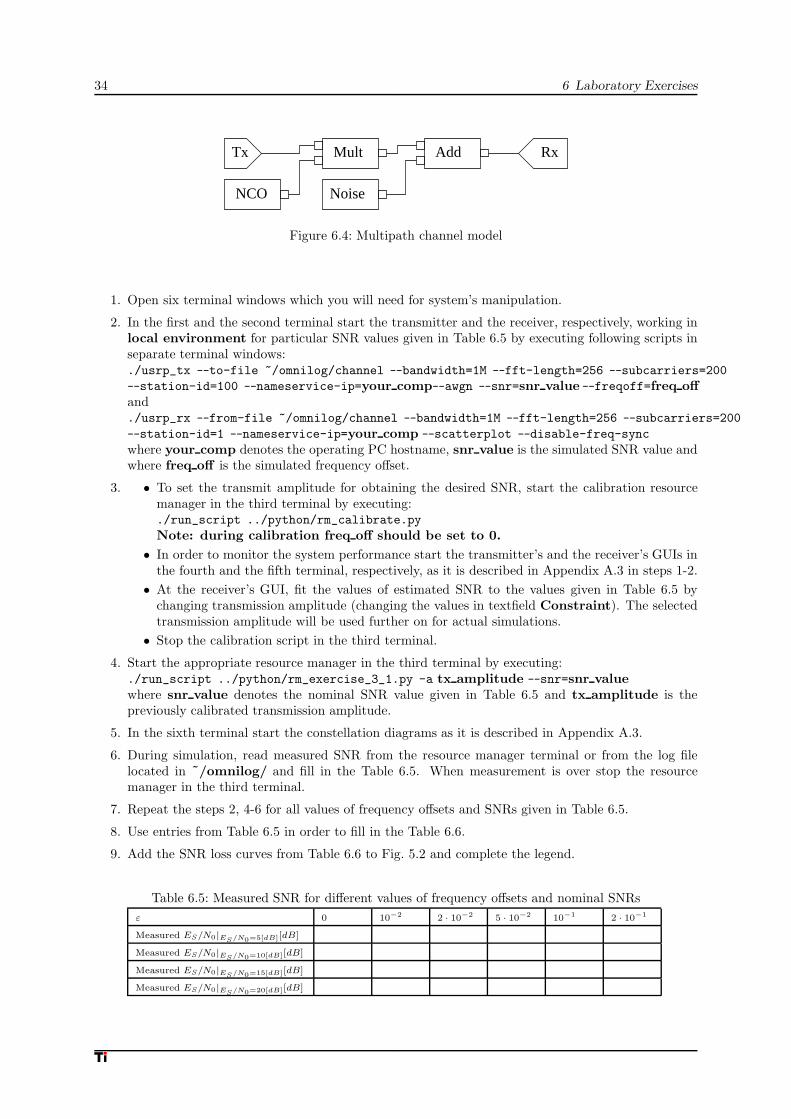
This task needs to be performed on a single PC. The corresponding simulation model of wireless channelin the presence of AWGN and CFO is shown in Fig. 6.4.


NCO

Mult Add

Noise

Tx Rx

Figure 6.4: Multipath channel model

1. Open six terminal windows which you will need for system’s manipulation.


--station-id=100 --nameservice-ip=your comp--awgn --snr=snr value --freqoff=freq offand./usrp_rx --from-file ~/omnilog/channel --bandwidth=1M --fft-length=256 --subcarriers=200

--station-id=1 --nameservice-ip=your comp --scatterplot --disable-freq-sync

where your comp denotes the operating PC hostname, snr value is the simulated SNR value andwhere freq off is the simulated frequency offset.

3. • To set the transmit amplitude for obtaining the desired SNR, start the calibration resourcemanager in the third terminal by executing:./run_script ../python/rm_calibrate.py

Note: during calibration freq off should be set to 0.

• In order to monitor the system performance start the transmitter’s and the receiver’s GUIs inthe fourth and the fifth terminal, respectively, as it is described in Appendix A.3 in steps 1-2.





6. During simulation, read measured SNR from the resource manager terminal or from the log filelocated in ˜/omnilog/ and fill in the Table 6.5. When measurement is over stop the resourcemanager in the third terminal.

7. Repeat the steps 2, 4-6 for all values of frequency offsets and SNRs given in Table 6.5.

8. Use entries from Table 6.5 in order to fill in the Table 6.6.

9. Add the SNR loss curves from Table 6.6 to Fig. 5.2 and complete the legend.

Table 6.5: Measured SNR for different values of frequency offsets and nominal SNRs

ε 0 10−2 2 · 10−2 5 · 10−2 10−1 2 · 10−1

Measured ES/N0|ES/N0=5[dB][dB]





Table 6.6: SNR losses for different values of frequency offsets and nominal SNRs

ε 10−2 2 · 10−2 5 · 10−2 10−1 2 · 10−1





10. Compare the obtained curves to those derived from the analytical model. How much do they differand why?

6.4.2 Real-time Transmission

This task needs to be performed on two PCs.

1. On transmitter’s PC in the first terminal start the transmitter by executing:./usrp_tx -f frequency --bandwidth=1M --fft-length=256

--subcarriers=200 --station-id=100 --nameservice-ip=comp 1where comp 1 is the name of the transmitting PC while transmission frequency depends on thedaughterboard type of your USRP. It will be given to you by the supervisors.

2. In order to use a name service which runs on a transmitter’s PC, on a receiver’s PC make a omniorbconfiguration file which will be stored in ˜/omnilog/ by executing./mk_configuration comp 1

3. On receiver’s PC set the omniorb configuration fileexport OMNIORB_CONFIG=~/omnilog/omniORB-comp 1.cfgNote: this action needs to be repeated in all active terminal windows on the receiver’sPC.

4. On the receiver’s PC start the receiver in the first terminal by executing:./usrp_rx -f frequency --bandwidth=1M --fft-length=256 --subcarriers=200

--station-id=1 --nameservice-ip=comp 1 --scatterplot --log-freq-off

5. To set the transmit amplitude for obtaining the desired SNR value, on transmitter’s PC in thesecond terminal start the calibration resource manager by executing:./run_script ../python/rm_calibrate.py

6. In order to monitor the system performance start the transmitter’s GUI in the third terminal ontransmitter’s PC and the receiver’s GUIs in the second terminal receiver’s PC, as it is described inAppendix A.3.

7. At the receiver’s GUI, fit the values of estimated SNR to 10 dB by changing transmission amplitude(changing the values in textfield Constraint and rx gain). The selected transmission amplitudewill be used further on for actual simulations.

8. Stop the calibration script.

9. Start the appropriate resource manager in the second terminal on transmitter’s PC by executing:./run_script ../python/rm_exercise_3_2.py -a tx amplitude --snr=10

where tx amplitude is the previously calibrated transmission amplitude.

10. In the third terminal on receiver’s PC start the constellation diagrams as it is described in Ap-pendix A.3.

11. Stop the receiver after about ten seconds and open the log file by executing:gr_plot_float.py ~/omnilog/freq off.float

12. Read the estimated frequency offset ε from the figure and calculate frequency offset fd in Hz using(2.5). Note that the bandwidth you use as transmission parameter corresponds to 1/Ts.

13. Add measured frequency offset fd to frequency previously used for real-time transmission and startthe receiver with the new corrected frequency.


14. Stop the receiver after about ten seconds and open the log file by executing:gr_plot_float.py ~/omnilog/freq off.float

15. What is the new value of the estimated frequency offset?

16. Conclude the results.

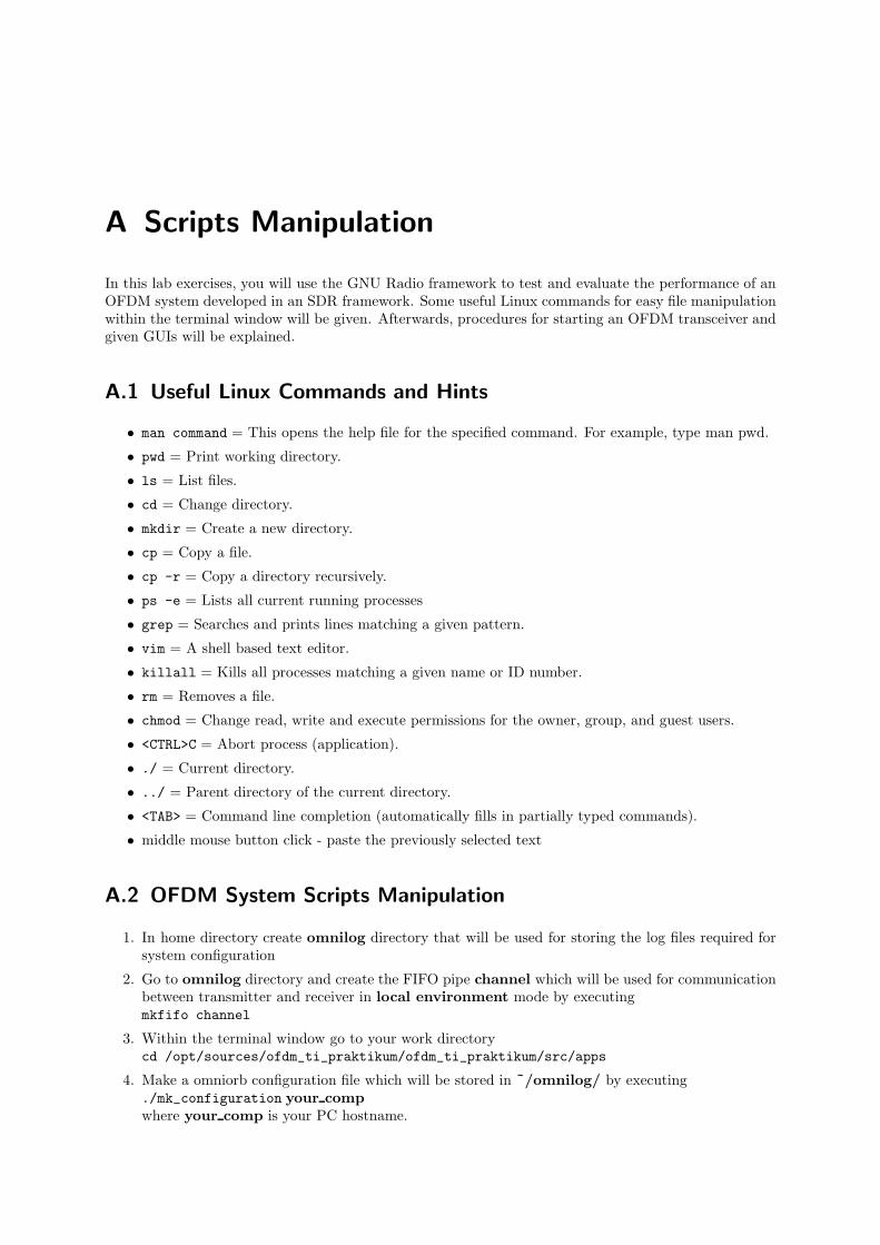
A Scripts Manipulation

In this lab exercises, you will use the GNU Radio framework to test and evaluate the performance of anOFDM system developed in an SDR framework. Some useful Linux commands for easy file manipulationwithin the terminal window will be given. Afterwards, procedures for starting an OFDM transceiver andgiven GUIs will be explained.

A.1 Useful Linux Commands and Hints

• man command = This opens the help file for the specified command. For example, type man pwd.

• pwd = Print working directory.

• ls = List files.

• cd = Change directory.

• mkdir = Create a new directory.

• cp = Copy a file.

• cp -r = Copy a directory recursively.

• ps -e = Lists all current running processes

• grep = Searches and prints lines matching a given pattern.

• vim = A shell based text editor.

• killall = Kills all processes matching a given name or ID number.

• rm = Removes a file.

• chmod = Change read, write and execute permissions for the owner, group, and guest users.

• <CTRL>C = Abort process (application).

• ./ = Current directory.

• ../ = Parent directory of the current directory.

• <TAB> = Command line completion (automatically fills in partially typed commands).

• middle mouse button click - paste the previously selected text

A.2 OFDM System Scripts Manipulation

1. In home directory create omnilog directory that will be used for storing the log files required forsystem configuration

2. Go to omnilog directory and create the FIFO pipe channel which will be used for communicationbetween transmitter and receiver in local environment mode by executingmkfifo channel

3. Within the terminal window go to your work directorycd /opt/sources/ofdm_ti_praktikum/ofdm_ti_praktikum/src/apps

4. Make a omniorb configuration file which will be stored in ˜/omnilog/ by executing./mk_configuration your compwhere your comp is your PC hostname.

40 A Scripts Manipulation

5. Start the CORBA name and event service by executing the script./Setup_Local_Environment

Note: ignore the warning messages.

6. Export environment variables. /opt/gnuradio/bin/environment

7. In order to set OMNIORB configuration file typeexport OMNIORB_CONFIG=~/omnilog/omniORB-your comp.cfgNote: last two actions need to be repeated in all active terminals.

8. To check if name service is correctly running typenameclt list

and the list of initiated name clients should be shown in the terminal window.

9. Transmitter (Tx) is started by typing./usrp_tx

Prior to actually execute the script, take a look at options that can be configured from commandline by typing./usrp_tx --help

Here is the list of options:

• h, --help show this help message and exit

• -f FREQ, --freq=FREQ set Tx and/or Rx frequency to FREQ [default=none]

• -which-usrp=WHICH_USRP select USRP box to use

• --from-file=FROM_FILE Sent recorded stream with USRP

• --to-file=TO_FILE Record transmitter to disk, not being sent to USRP

• -e INTERFACE, --interface=INTERFACE select Ethernet interface, default is eth0

• -m MAC_ADDR, --mac-addr=MAC_ADDR select USRP by MAC address, default is auto-select

• --usrp2 Use USRP2 Interface

• --fft-length=FFT_LENGTH set the number of FFT bins [default=512]

• -a AMPL, --rms-amplitude=AMPL set total bandwidth. [default=500k]

• --tx-freq=FREQ set transmit frequency to FREQ [default=none]

• --snr=SNR Simulate AWGN channel

• --freqoff=FREQOFF Simulate frequency offset [default=none]

• --samplingoffset=SAMPLINGOFFSET Simulate sampling frequency offset [default=none]

• --awgn Enable static AWGN power for BER measurement

• --data-blocks=DATA_BLOCKS Set the number of data blocks per OFDM frame [default=9]

• --subcarriers=SUBCARRIERS Set the number of occupied FFT bins. Default: FFT windowsize - Pilot Subcarriers

• --cp-length=CP_LENGTH Set the unique ID number for each node within the system

• --station-id=STATION_ID Set IP address or hostname that hosts the CORBA NameService

• --nameservice-ip=NAMESERVICE_IP

• --nameservice-port=NAMESERVICE_PORT Set access port to NameService

• --log enable file logs [default=False]

• --debug Enable debugging mode [default=False]

10. For example, in order to start transmission over USRP, execute the script with following parameters./usrp_tx -f 2.45G --bandwidth=2M --fft-length=256 --subcarriers=200

--station-id=100 --nameservice-ip=your comp

11. Similarly, in order to start transmission in local environment in AWGN channel with SNR = 20dB, execute the script with following parameters./usrp_tx --to-file channel --bandwidth=2M --fft-length=256 --subcarriers=200

--station-id=100 --nameservice-ip=your comp --awgn --berm --snr=20.

A.2 OFDM System Scripts Manipulation 41

12. Receiver (Rx) is started by typing./usrp_rx

Prior to actually execute the script, take a look at options that can be configured from commandline by typing./usrp_rx --help

Here is the list of options:

• h, --help show this help message and exit

• -f FREQ, --freq=FREQ set Tx and/or Rx frequency to FREQ [default=none]

• --which-usrp=WHICH_USRP select USRP box to use

• --rx-gain=GAIN set receiver gain in dB [default=midpoint]. See also --show-rx-gain-range

• --show-rx-gain-range print min and max Rx gain available on selected daughterboard

• --from-file=FROM_FILE Run Receiver on recorded stream

• --to-file=TO_FILE Record stream from USRP to disk, no processing

• -e INTERFACE, --interface=INTERFACE select Ethernet interface, default is eth0

• -m MAC_ADDR, --mac-addr=MAC_ADDR select USRP by MAC address, default is auto-select

• --usrp2 Use USRP2 Interface

• --event-rxbaseband Enable RX baseband via event channel alps

• --fft-length=FFT_LENGTH set the number of FFT bins [default=512]

• --disable-ctf-enhancer Disable Enhancing the MSE of CTF

• --scatterplot Enable the GUI interface for showing constellation diagrams of the receivedsignal

• --bandwidth=BANDWIDTH set total bandwidth. [default=500k]

• --rx-freq=FREQ set receive frequency to FREQ [default=none]

• --online-work Force the OFDM receiver to work during file record [default=False]

• --data-blocks=DATA_BLOCKS set the number of data blocks per OFDM frame [default=9]

• --subcarriers=SUBCARRIERS set the number of occupied FFT bins. Default: FFT windowsize - Pilot Subcarriers

• --cp-length=CP_LENGTH set the number of bits in the cyclic prefix. Default: 12.5

• --station-id=STATION_ID Set the unique ID number for each node within the system

• --nameservice-ip=NAMESERVICE_IP Set IP address or hostname that hosts the CORBANameService

• --nameservice-port=NAMESERVICE_PORT Set access port to NameService

• --log Enable file logs [default=False]

• --log-freq-off Enable log of frequency offset estimation

• --debug Enable debugging mode [default=False]

• --disable-freq-sync Disabling frequency synchronization stage

• --disable-equalization Disabling equalization stage

• --disable-phase-tracking Disabling phase tracking stage

• --disable-time-sync Disabling time synchronization stage

13. For example, in order to start reception over USRP, execute the script with following parameters./usrp_rx -f 2.45G --bandwidth=2M --fft-length=256 --subcarriers=200


14. Similarly, in order to start transmission in local environment in AWGN channel, execute the scriptwith following parameters./usrp_rx --from-file channel --bandwidth=2M --fft-length=256 --subcarriers=200


15. Resource manager (that will be implements in different scripts for different exercises) is started byexecuting the script./run_script ../python/exercise_x_x.py

42 A Scripts Manipulation

A.3 GUI Scripts Manipulation

1. In order to start system’s GUIs docd /opt/sources/ofdm_ti_praktikum/ofdm_ti_praktikum/src/qt/gui

2. Tx’s GUI is started by executing./qtgui --tx --nameservice=your comp

3. Rx’s GUI is started by executing./qtgui --rx --nameservice=your comp

4. Constellation plots can be observed by going into directorycd /opt/sources/ofdm_ti_praktikum/ofdm_ti_praktikum/src/qt/scatterplot

and executing the script./scatterplot-gui

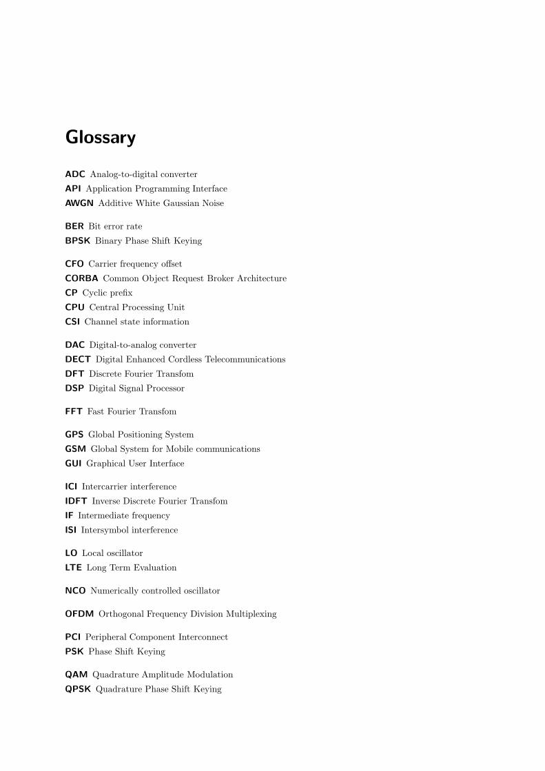
Glossary

ADC Analog-to-digital converter

API Application Programming Interface

AWGN Additive White Gaussian Noise

BER Bit error rate

BPSK Binary Phase Shift Keying

CFO Carrier frequency offset

CORBA Common Object Request Broker Architecture

CP Cyclic prefix

CPU Central Processing Unit

CSI Channel state information

DAC Digital-to-analog converter

DECT Digital Enhanced Cordless Telecommunications

DFT Discrete Fourier Transfom

DSP Digital Signal Processor

FFT Fast Fourier Transfom

GPS Global Positioning System

GSM Global System for Mobile communications

GUI Graphical User Interface

ICI Intercarrier interference

IDFT Inverse Discrete Fourier Transfom

IF Intermediate frequency

ISI Intersymbol interference

LO Local oscillator

LTE Long Term Evaluation

NCO Numerically controlled oscillator

OFDM Orthogonal Frequency Division Multiplexing

PCI Peripheral Component Interconnect

PSK Phase Shift Keying

QAM Quadrature Amplitude Modulation

QPSK Quadrature Phase Shift Keying

44 Glossary

RF Radio frequency

SDR Software Defined Radio

SER Symbol error rate

SNR Signal-to-noise ratio

USRP Universal Software Radio Peripheral

WiMAX Worldwide Interoperability for Microwave Access

WLAN Wireless Local Access Network

Index

ADC, 7, 17API, 19AWGN, 3, 6, 12, 13, 29, 30, 34

BER, 13–15, 23, 24BPSK, 12, 13

CFO, 7, 34Channel frequency response, 9, 12Channel impulse response, 6CORBA, 23, 24, 29CP, 5, 6CSI, 23, 24

DAC, 17DECT, 18DFT, 3, 5, 7, 8DSP, 17

FFT, 3, 23Frequency offset, 7, 9, 10, 21, 26, 27, 33, 34, 36

GNU Radio, 3, 18–21, 23, 24, 39GPS, 18GSM, 18GUI, 24

ICI, 7IDF, 5IDFT, 5, 6ISI, 3, 5

LO, 7LTE, 12

OFDM, 3, 5–7, 10–12, 23, 39

PSK modulation, 6, 12–14Python, 20, 21

QAM modulation, 6, 14, 15QPSK modulation, 12, 15

SDR, 3, 17, 18, 23, 39SER, 14, 15SNR, 6, 10, 13, 14, 23–26, 29–32, 34, 35SNR loss, 10

Time offset, 10, 23

USRP, 3, 19, 23, 24, 29, 30, 35

WiMAX, 15WLAN, 15

46 Index

Bibliography

[Aur09] Dominik Auras. GNU Radio Implementierungen zur Synchronisierung von OFDM-Systemen.Studienarbeit, RWTH Aachen, 2009.

[Erg09] Mustafa Ergen. Mobile Broadband - Including WiMAX and LTE. Springer Publishing Com-pany, Incorporated, 2009.

[GNUrg] ”Object Management Group”, http://www.omg.org/.

[GNUpp] IT++, http://sourceforge.net/apps/wordpress/itpp.

[GNUac] ”GNU Radio”, http://gnuradio.org/trac.

[Gol05] Andrea Goldsmith. Wireless Communications. Cambridge University Press, New York, NY,USA, 2005.

[LS06] Ye Li and Gordon L. Stuber. Orthogonal Frequency Division Multiplexing for Wireless Commu-nications (Signals and Communication Technology). Springer-Verlag New York, Inc., Secaucus,NJ, USA, 2006.

[Mar03] Alex Martelli. Python in a Nutshell. A Desktop Quick Reference. O’Reilly & Associates, 1edition, 2003.

[Mey98] Scott Meyers. Effektiv C++ programmieren. Addison Wesley, 1998.

[Mey99] Scott Meyers. Mehr Effektiv C++ programmieren. Addison Wesley, 1999.

[Mey01] Scott Meyers. Effective STL. Addison Wesley, 2001.

[Mit06] Joseph III Mitola. Cognitive Radio Architecture: The Engineering Foundations of Radio Xml.Wiley-Interscience, New York, NY USA, 2006.

[MR97] Thomas J. Mowbray and William A. Ruh. Inside CORBA. Addison Wesley, 1997.

[Mue08] Andreas Mueller. DAB, Software Receiver Implementation. Semester Thesis, ETH Zurich,2008.

[OHE97] Robert Orfali, Dan Harkey, and Jeri Edwards. Instant CORBA. John Wiley & Sons, 1997.

[PMK07] Man-on Pun, Michele Morelli, and C. C. Jay Kuo. Multi-Carrier Techniques For BroadbandWireless Communications: A Signal Processing Perspectives. Imperial College Press, London,UK, UK, 2007.

[Rou08] Tony J. Rouphael. RF and Digital Signal Processing for Software-Defined Radio: A Multi-Standard Multi-Mode Approach. Newnes, Newton, MA, USA, 2008.

[SA07] Herb Sutter and Andrei Alexandrescu. C++ Coding Standards. Addison Wesley, Boston, Mas-sachusetts, USA, 5 edition, July 2007.

[Str00] Bjarne Stroustrup. Die C++ Programmiersprache. Addison Wesley, 2000.

[ZAM09] Milan Zivkovic, Dominik Auras, and Rudolf Mathar. Reconfigurable framework for adaptiveofdm transmission. In WINTECH ’09: Proceedings of the 4th ACM international workshop onExperimental evaluation and characterization, pages 91–92, New York, NY, USA, 2009. ACM.

lab exercises - rwth aachen university · lab exercises modules: ... a way that attenuation across...

Documents