lab 2: modern legos and tinkertoys - harvard universitysites.fas.harvard.edu/~lsci1a/lab2.pdf ·...

Life Sciences 1a Laboratory – Fall 2006

34

Lab 2: Modern Legos and Tinkertoys (AKA Computer Modeling with PyMol #1) Goals: The objective of this lab is to provide you with an understanding of:

1. How to use PyMol at a basic level. 2. The different representations used by scientists when working with

biological polymers. 3. How biological polymers assemble and fold to form distinct

macromolecules. 4. The variety of macromolecular shapes that is possible through the use of

a finite number of building blocks. 5. The key structural features of DNA and proteins, and how they enable

each macromolecule’s respective functions. Introduction: As you have learned in the lectures, some of the most important molecules associated with life are polymers. Polymers are chains composed of many repeating units called monomers, which act as the basic chemical building blocks. By stringing together a variety of these monomeric molecules into a specific sequence, one can generate a macromolecule that is capable of performing specific functions that are essential to maintaining life. Some key functions include storing genetic information, converting genetic information into useful structures, regulating cellular function, and accelerating otherwise slow chemical reactions.

Biological Polymer: Monomer: Nucleic Acids (DNA, RNA) Nucleotides Protein Amino acids Carbohydrates Saccharides Considering the relatively small quantity of available building blocks, it is astonishing to reflect on the seemingly endless number of distinct and otherwise amazing functions that these macromolecules perform! In order to understand how these biological macromolecules are able to accomplish these feats, we must first understand how these polymers fold and assemble into functional shapes. Using a variety of modern methods (which are beyond the scope of this course), scientists are able to determine the distinct 3-D molecular shape of a macromolecule. Scientists can then make educated guesses about how they function, based on the location of key molecular components. This information is vital to improving our understanding of diseases at a molecular level, and for identifying potential drug targets.


35

A prime example of the cooperative nature of science, the Protein Data Bank (“PDB”) http://www.rcsb.org/pdb/Welcome.do is an online repository of 3-D biological structural data; anytime the 3-D structure of a biological molecule is solved, its coordinates are promptly deposited into this database, where it is made available to all researchers. All that is required is a simple computer program to enable scientists to manipulate the coordinates in a clear and useful manner. We will be using a new program called PyMol to examine some of these remarkable 3-D structures. PyMol is a free software tool that allows researchers to download PDB files and work with them in a variety of representations, so that they are able to manipulate the structures easily and extract useful information for their research. We have generated specific scripts for you to work with. Procedures: The lab is composed of six sections; each section will utilize a PDB coordinate file and an accompanying script. The questions will be due one week from the day of the lab. Section 1: Introduction to PyMol a. Basic Manipulations

• To begin using PyMol, open up the folder titled “1_Intro,” then double-click on the PyMol file labeled “Intro.pml.” This will automatically open up the PyMol program, and load up the coordinates for the DNA structure.

At this point, PyMol should have loaded up into two windows: an “external” interface on top, and a larger “viewer” window below it. For our needs, we will focus exclusively on the “viewer” window. You can maximize this window if you choose (this can be done by clicking the grey “+” button at the top left corner of the window). In the viewer window, you will see your first structure; it should look something like this:


36

This image represents the structure of B-DNA in what we call “sticks” form; each of the lines represents a covalent bond. Each element is also colored differently. We will discuss different representations shortly.

• Try manipulating the DNA molecule by clicking on it with your mouse; the basic controls are as follows:

• To “Move” an object, you must click on the object using the wheel as a button. Rotating the wheel simply controls the “Z-axis clipping plane” for the viewer (this feature allows you to control how much thick your viewing plane is… helpful for looking at larger structures).

• Double-clicking the Move button will re-center the viewer on the clicked point.

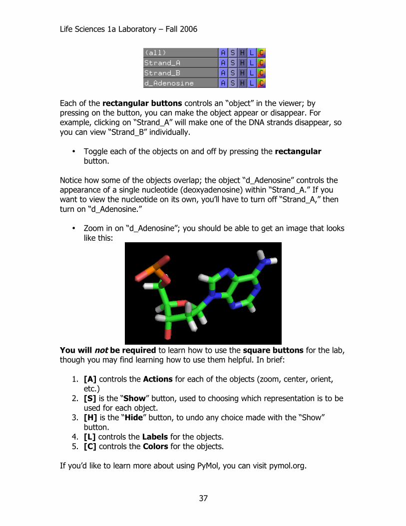
Practice using all three functions; once you have a feel for how to manipulate each object, you can move on to the next section. b. Turning on / off the Objects On the right side of the viewer window, you will notice a series of rectangular buttons with names in them, as well as a series of square buttons ([A], [S], [H], [L], and [C]) for each rectangular button:


37

Each of the rectangular buttons controls an “object” in the viewer; by pressing on the button, you can make the object appear or disappear. For example, clicking on “Strand_A” will make one of the DNA strands disappear, so you can view “Strand_B” individually.

• Toggle each of the objects on and off by pressing the rectangular button.

Notice how some of the objects overlap; the object “d_Adenosine” controls the appearance of a single nucleotide (deoxyadenosine) within “Strand_A.” If you want to view the nucleotide on its own, you’ll have to turn off “Strand_A,” then turn on “d_Adenosine.”

• Zoom in on “d_Adenosine”; you should be able to get an image that looks like this:

You will not be required to learn how to use the square buttons for the lab, though you may find learning how to use them helpful. In brief:

1. [A] controls the Actions for each of the objects (zoom, center, orient, etc.)

2. [S] is the “Show” button, used to choosing which representation is to be used for each object.

3. [H] is the “Hide” button, to undo any choice made with the “Show” button.

4. [L] controls the Labels for the objects. 5. [C] controls the Colors for the objects.

If you’d like to learn more about using PyMol, you can visit pymol.org.


38

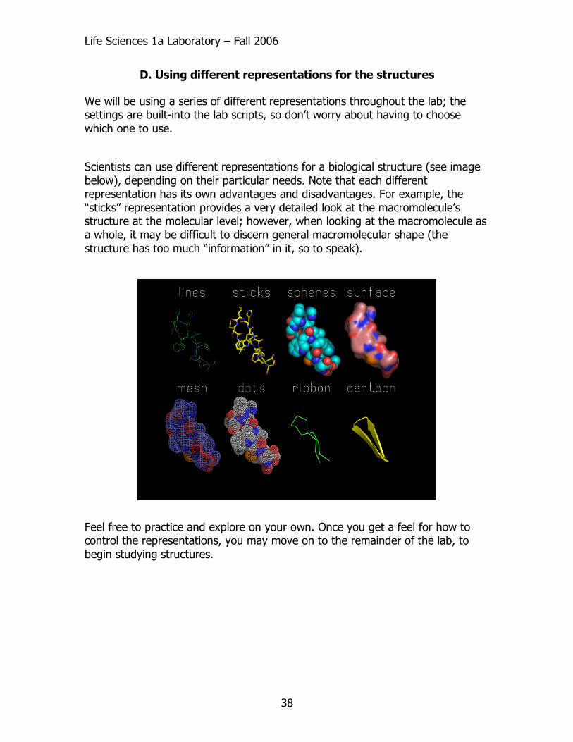
D. Using different representations for the structures We will be using a series of different representations throughout the lab; the settings are built-into the lab scripts, so don’t worry about having to choose which one to use.

Scientists can use different representations for a biological structure (see image below), depending on their particular needs. Note that each different representation has its own advantages and disadvantages. For example, the “sticks” representation provides a very detailed look at the macromolecule’s structure at the molecular level; however, when looking at the macromolecule as a whole, it may be difficult to discern general macromolecular shape (the structure has too much “information” in it, so to speak).

Feel free to practice and explore on your own. Once you get a feel for how to control the representations, you may move on to the remainder of the lab, to begin studying structures.


39

Section 2: Nucleic Acids Basics

• Open up the folder titled “2_Nucleic_Acids_Basics,” then double-click on the PyMol file labeled “NucleicAcids.pml.” This will automatically open up the PyMol program, and load up the coordinates for the DNA structure.

The first image you will see is that of 2’ deoxyribose, a derivative of the sugar ribose.

• Try orienting the PyMol image so that the perspective aligns with those shown in the drawings. The numbering of the carbons is shown:

O

HO

OHHO

2' deoxyribose

5'4'

2'3'

1' O

HO

OHHO

ribose

5'4'

2'3'

1'

OH

Note the basic structure of the sugar; this acts as the backbone of DNA. Notice how the hydrogens are omitted in the program, similar to how hydrogens are typically omitted in organic structures.

As a convention, oxygen is colored red. Carbon, in this case, is colored green, though the color for carbon will vary throughout the lab, in order to allow for differentiation between structures.

• Turn off “Deoxyribose” and turn on “Nitrogen_Base.”

This will give you a basic view of adenine, one of the four nitrogen bases. Note that it is essentially planar in shape. You’ll also note that nitrogen is colored blue, another convention we’ll use throughout the lab. We’ll discuss the different nitrogen bases of DNA in detail shortly.

N

NNH

N

NH2

adenine

• Turn off “Nitrogen_Base” and turn on “d_Nucleoside.”

This will illustrate for you now nucleosides are assembled from a sugar and a nitrogen base. Since there are four available nitrogen bases for DNA, there are


40

four corresponding nucleosides for DNA. The “d” denotes that the sugar is 2’ deoxy.

1) At which carbon on deoxyribose did the nitrogen group substitute for one of the sugar oxygens?

• Turn off “d_Nucleoside” and turn on “d_Nucleotide.”

At this point, a 5’ phosphate group will be added onto the 5’ oxygen of the nucleoside. This unit is called the nucleotide, which is the basic building block (the “monomer”) of a nucleic acid. This particular one is deoxyadenosine, since adenine is used as the nitrogen base. Also note that phosphorous is colored orange.

O

PO

O

Ophosphate

• Turn off “d_Nucleotide” and turn on “Dinucleotide.”

You will see now how two nucleotides are strung together.

2) Which sugar oxygens do the phosphates link?

• Turn off “Dinucleotide” and turn on “Strand_A.”

Now that you have a basic understanding of how nucleotides are linked together, one can imagine linking several of them together for form a long, polymeric nucleic acid. Notice that, as the strand length increases, the strand begins to take on a rather helical shape. Also note that the nitrogen bases all point towards the “inside” of the helix. This forms the interface for the second strand of DNA.

• Turn on “Strand_B” (leave “Strand_A” on).

As you’ll recall from lecture, DNA is double stranded; the helical nature of the strands accommodates two strands running together.


41

3) Are the strands parallel, or anti-parallel? Identify the 5’ and 3’ ends of each strand.

• Turn on “Cartoon” (leave “Strand_A” and “Strand_B” on).

To simplify the backbone structure, scientists often use a representation called a “cartoon.” This makes the general structure of the DNA more easily discernable. Notice that the lines that appear along the sugar-phosphate backbone.

Cartoons are particularly useful for viewing larger structures, when “sticks” can get too cumbersome.

• Turn off “Strand_A,” “Strand_B,” and “Cartoon,” then turn on “Helix.”

To clarify the structure of the double helix, here is a “spheres” representation of the DNA strands, where we’ve colored one strand blue, and the other red. This makes the general shape of the helix easier to see.

4) Is the helix right-handed or left-handed?

Since there are two strands in a DNA helix, you’ll also notice that there are two “grooves” (the spaces between the two strands) that run the length of the DNA helix. Due to the asymmetry of the DNA backbone, one of these grooves is larger than the other. We call the larger groove the “major” groove, and the smaller one the “minor” groove.

As a general rule of thumb, small molecules that bind to DNA typically bind via the minor groove; proteins that bind to DNA typically bind through the major groove.

5) Identify the major and minor groove:


42

• Turn off “Helix” and turn on “Backbone.”

To clarify the structure of the DNA backbone, we’ve eliminated the bases, and have colored all the oxygens red, to emphasize their solvent accessibility.

• Turn on “Bases” (leave “Backbone” on).

Here, we see how the nitrogen bases fill out the interior of the DNA double helix. We’ve colored each of the four bases a different color (one color for each of the four bases).

N

NN

N

N

adenosine(dark blue)

N

NN

N

O

guanosine(light blue)

H

NH

H

H H

N

N

H

O

O

CH3thymidine(magenta)

N

N

N

O

cytidine(pink)

H H

We will be discussing the nature of this pairing in greater detail in the next section.

Also, take time to notice the stacking between the bases in the center of the helix. Note how closely the planar bases are oriented alongside each other; this is an important feature of the double helix, in relation to the hydrophobic effect we have discussed in lecture.


43


44

Section 3: DNA Hydrogen Bonding Basics

• Open up the folder titled “3_DNA_H_Bonding,” then double-click on the PyMol file labeled “H_Bonding.pml.” This will automatically open up the PyMol program, and load up the coordinates for the DNA structure.

The program will start with an image of DNA (“Strand_A” and “Strand_B”), just as you saw in the previous lab. There is, however, one significant difference. In this structure, we’ve included the hydrogens (white) into the structure, against convention. These hydrogens will allow us to see hydrogen bonding patterns more clearly. Take a moment to view DNA with the hydrogens represented.

• Turn off “Strand_A” and “Strand_B,” and turn on “d_Adenosine” and “d_Thymidine.”

Note how these two nucleotides, deoxyadenosine and deoxythymidine, always pair opposite each other (you can check this using “Strand_A” and “Strand_B” to view the entire DNA strand). This is abbreviated as an AT base pair. 6) Draw the base-pairing orientations of the nitrogen bases.

• Turn on “AT_H_Bonds”

This should add the hydrogen bonds into the image, represented as dotted yellow lines. 7) In this structure, how many hydrogen bonds are there between adenosine and thymidine? 8) Draw in the hydrogen bonds on your base-pairing drawing. Now let’s look at the base-pairing for the other set of nucleotides:

• Turn off “d_Adenosine,” “d_Thymidine,” and “AT_H_Bonds,” then turn on “d_Guanosine,” “d_Cytidine,” and “GC_H_Bonds.”

9) Draw the base-pairing orientations for guanosine and cytidine, including the hydrogen bonds. A and T are called complementary to each other. G and C are thus complements as well. Thus, a complementary strand is one that has perfect base complementation for each base of the original strand. Remember, DNA binds


45

antiparallel, so if both strands are written from a 5’ to 3’ direction, you must remember to account for the reverse in direction. For example, the complement of: 5’-GTTACGC-3’ would be 5’-GCGTAAC-3’.

10) What is the complement of the following strand: 5’-GACTAACTAG-3’? Before the structure of DNA was known, a scientist named Erwin Chargaff observed that, within an organism’s nucleus, the chemical content of A was always equal to the content of T, and the content of G was always equal to the content of C. However, the relative amount of A-T and G-C varied between organisms. This became known as “Chargaff’s Rule.” 11) In light of what you know, explain this observed phenomenon (in brief).


46

Section 4: Protein Basics

• Open up the folder titled “4_Protein_Basics,” then double-click on the PyMol file labeled “Protein_Basics.pml.” This will automatically open up the PyMol program, and load up the coordinates for Hemoglobin.

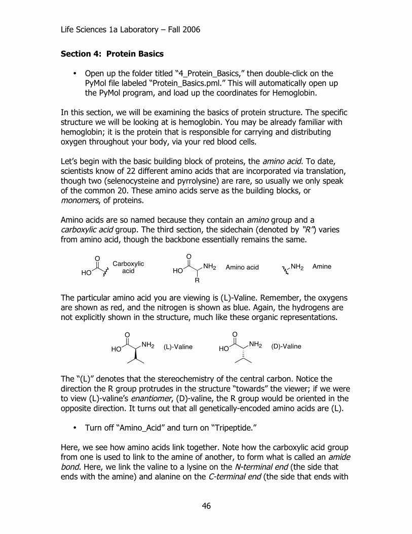
In this section, we will be examining the basics of protein structure. The specific structure we will be looking at is hemoglobin. You may be already familiar with hemoglobin; it is the protein that is responsible for carrying and distributing oxygen throughout your body, via your red blood cells. Let’s begin with the basic building block of proteins, the amino acid. To date, scientists know of 22 different amino acids that are incorporated via translation, though two (selenocysteine and pyrrolysine) are rare, so usually we only speak of the common 20. These amino acids serve as the building blocks, or monomers, of proteins. Amino acids are so named because they contain an amino group and a carboxylic acid group. The third section, the sidechain (denoted by “R”) varies from amino acid, though the backbone essentially remains the same.

HO

O

NH2HO

OCarboxylic

acidAmineNH2Amino acid

R

The particular amino acid you are viewing is (L)-Valine. Remember, the oxygens are shown as red, and the nitrogen is shown as blue. Again, the hydrogens are not explicitly shown in the structure, much like these organic representations.

HO

O

NH2 (L)-Valine HO

O

NH2 (D)-Valine

The “(L)” denotes that the stereochemistry of the central carbon. Notice the direction the R group protrudes in the structure “towards” the viewer; if we were to view (L)-valine’s enantiomer, (D)-valine, the R group would be oriented in the opposite direction. It turns out that all genetically-encoded amino acids are (L).

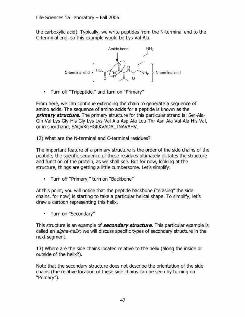
• Turn off “Amino_Acid” and turn on “Tripeptide.” Here, we see how amino acids link together. Note how the carboxylic acid group from one is used to link to the amine of another, to form what is called an amide bond. Here, we link the valine to a lysine on the N-terminal end (the side that ends with the amine) and alanine on the C-terminal end (the side that ends with


47

the carboxylic acid). Typically, we write peptides from the N-terminal end to the C-terminal end, so this example would be Lys-Val-Ala.

NH

OHN

OO

HONH2

NH2Amide bond

N-terminal endC-terminal end

• Turn off “Tripeptide,” and turn on “Primary” From here, we can continue extending the chain to generate a sequence of amino acids. The sequence of amino acids for a peptide is known as the primary structure. The primary structure for this particular strand is: Ser-Ala-Gln-Val-Lys-Gly-His-Gly-Lys-Lys-Val-Ala-Asp-Ala-Leu-Thr-Asn-Ala-Val-Ala-His-Val, or in shorthand, SAQVKGHGKKVADALTNAVAHV. 12) What are the N-terminal and C-terminal residues? The important feature of a primary structure is the order of the side chains of the peptide; the specific sequence of these residues ultimately dictates the structure and function of the protein, as we shall see. But for now, looking at the structure, things are getting a little cumbersome. Let’s simplify:

• Turn off “Primary,” turn on “Backbone” At this point, you will notice that the peptide backbone (“erasing” the side chains, for now) is starting to take a particular helical shape. To simplify, let’s draw a cartoon representing this helix.

• Turn on “Secondary” This structure is an example of secondary structure. This particular example is called an alpha-helix; we will discuss specific types of secondary structure in the next segment. 13) Where are the side chains located relative to the helix (along the inside or outside of the helix?). Note that the secondary structure does not describe the orientation of the side chains (the relative location of these side chains can be seen by turning on “Primary”).


48

• Turn off “Backbone” and “Secondary,” turn on “Tertiary.” Now, if we combine an entire series of secondary elements, we get a large, compact structure called the tertiary structure of the protein. At this level of resolution, you’ll notice the shape of the protein is somewhat irregular. It is this shape that allows each protein to carry out its particular function with great efficiency; the shape provides an optimal scaffold for the required job.

• Turn on “Full_Backbone.” Notice how well the cartoon aligns with the “cartoon” of the tertiary structure; again, the cartoon is a convenient simplification of the overall structure of the protein. Let’s see what the protein looks like without simplification:

• Turn off “Full_Backbone” and “Tertiary,” turn on “Sticks_Rep” 14) Why is this a poor representation to use when analyzing the structure of an entire protein? Let’s examine another type of representation.

• Turn on “Surface_Rep” This is called a surface representation. This represents the actual volume and net shape the protein occupies… what the solvent “sees,” if you will. It provides a great sense of what the actual surface of the protein is like in any given area. 15) In what situations would a surface representation be optimal to use? Explain.

• Turn off “Surface_Rep” and “Sticks_Rep,” turn on “Tertiary.” Now, what happens if multiple domains work in concert?

• Turn off “Tertiary,” and turn on “Quaternary” Each of these domains (differently colored) are virtually identical in structure and sequence; sometimes, protein structures are bound together to form a single, functionally redundant unit. 16) How many polypeptide chains comprise a complete hemoglobin molecule? As we’ve mentioned earlier, hemoglobin acts as an oxygen carrier. But where does it carry the oxygen? Sometimes, proteins need additional structural units to perform their duties, if the standard battery of amino acid sidechains isn’t


49

adequate. At this point, proteins utilize a small molecule, called a cofactor, to assist.

• Turn on “Cofactor” In this particular case, the cofactor is a porphyrin ring, a large ring with a metal ion in the center (here, iron is used as the central ion). Notice that each chain gets its own cofactor. To see where the oxygen gets bound to the ring, turn on “oxygen”

• Turn on “Oxygen” At this point, we want to stress that the ability of hemoglobin to bind these cofactors, and thus oxygen, is dependent on the structure of the protein itself. And, as you’ve seen, this structure is determined by the sequence of amino acids that combine in a distinct order to form the protein. Again, it is the sequence of amino acids that dictates the properties and functions of a protein.


50

Section 5: Protein Secondary Structure

• Open up the folder titled “5_Secondary_Structure,” then double-click on the PyMol file labeled “Secondary_Structure.pml.” This will automatically open up the PyMol program, and load up the coordinates for Top7.

In this brief section, we will be examining the different basic varieties of protein secondary structure, and how cartoons are used to simplify proteins. This particular protein that you are looking at, in glorious stick form, is called Top7. This is actually not a natural protein, but rather a protein that was designed by computational scientists in the David Baker group. As you might have guessed, predicting the structure of a protein from its full primary sequence (or designing a primary sequence that will fold into a desired structure) is very difficult to do. So difficult, in fact, that scientists are only now just starting to have success, with the help of powerful computers. Stick representation is a bit noisy, so let’s simplify the protein to its backbone, as we’ve done previously.

• Turn off “Protein_Sticks,” turn on “Backbone.” Already, you can start to see some of the basic motifs of secondary structure; eliminating the side groups alone does much to simplify a structure. Let’s examine each of these motifs in greater detail.

• Turn on “Helix_Sticks” Now, these particular amino acids form rather helical secondary structures, exactly like those we saw in hemoglobin. Thus, we will simplify them in cartoon mode as helices. These structures are called alpha-helices, and are quite common in proteins. Here, we’ve colored them magenta for clarity.

• Turn off “Helix_Sticks,” turn on “A_Helix.” 17) Are these helices right-handed or left-handed? So what causes these peptides to take on a helical shape? Of course, the answer is very complex, but it turns out that, by forming an alpha helix, the amino acids are able to form a series of hydrogen bonds that help to stabilize the structure. Certain amino acids favor this secondary structure more than others.


51

18) Why might the incorporation of the amino acid proline disrupt helix formation? Now, for the straight sections in the back

• Turn on “Sheet_Sticks” These strands take on a slightly different shape than those seen in helices; rather than curling, these peptidic strands form long, straight sheets when aligned with each other. Thus, we simplify them in cartoon mode as beta-strands, which combine to form beta-sheets. We’ve illustrated the sheets here in blue.

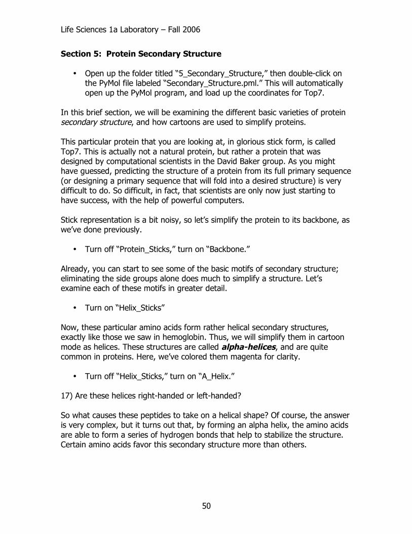
• Turn off “Sheet_Sticks,” turn on “B_Sheet.” Notice how sheets are represented in cartoon mode using long, flattened arrows; the arrows provide directionality for the sheets. Since amino acids, by convention, are written from N-terminal end to C-terminal end, the arrows point in the C-terminal direction of the peptide strands. Similarly to alpha-helices, the driving force for formation of beta-sheets is the formation of stabilizing hydrogen bonds between the neighboring strands. Again, certain amino acids favor beta-sheet formation over other types of secondary structure.


52

In order for a beta-sheet to form, it needs several flat peptide strands to align together to form a flat sheet. Since aligned sheets can run “in the same direction” or “in the opposite direction,” we describe beta sheets as being either parallel or anti-parallel. 19) Are the beta-sheets in this structure parallel or anti-parallel? Now, what about the protein segments that connect these secondary structure elements?

• Turn on “Loop_Sticks.” These segments do not exhibit a uniform structure, as seen in the previous two motifs; rather, they serve simply to connect the other motifs together. In some protein structures, these segments are so “disordered” that they do not even appear in the crystal structure at all.

• Turn off “Loop_Sticks” and turn on “Loops.” Thus, we simplify these as loops, which are depicted as simple ribbons (in this case, yellow).

• Turn on “C_Term_Sticks” and “N_Term_Sticks.” In addition to loops, the N-terminal and C-terminal ends of the peptide strand are often lacking in definite structure as well; these segments are also often missing in many crystal structures due to their wealth of disorganization. These termini are generally depicted in a similar manner as loops, though they don’t actually connect anything. Rather, they signify the “beginning” and “end” of the protein.


53

• Turn off “C_Term_Sticks” and “N_Term_Sticks,” turn on “C_Term” and N_Term.”

And here, we now see we have our entire protein represented in secondary structure elements, via a cartoon representation. To see the protein as a single cartoon, turn off all the other elements, and turn on “Protein.”

• Turn off all elements by hitting the “(all)” button at the top; turn on “Protein.”

Notice how the secondary motifs combine to generate a unique tertiary structure for the protein.


54

Section 6: Bulk Water

• Open up the folder titled “6_Bulk_Water,” then double-click on the PyMol file labeled “Water.pml.” This will automatically open up the PyMol program, and load up the coordinates for bulk water.

When scientists use the phrase “bulk water,” we are describing the behavior of water in absence of any other molecules to interact with. Of course, the “structure” of water is somewhat hard to define; since it is composed of a multitude of free molecules, water is a highly dynamic system, meaning it is rapidly changing between different states. To reduce bulk water to a single static image may belie many of the complexities that are important when considering the properties of a solvent. The simplification that results from converting any dynamic system (proteins included) into a single static image is something that must always be considered when viewing any crystal structure. As you might have already guessed, this particular set of coordinates is not from an x-ray crystal structure, but rather, a “simulation” of how bulk water is structured at any given instant. The exact nature of bulk water is still under debate in theoretical physical chemistry circles; here we present one representation. Here we can see an aliquot of water represented in “sticks” form. We’ve chosen to include the hydrogens in the representation. Otherwise, we wouldn’t be able to show water in sticks format at all, since the oxygen would appear to have nothing bonded to it! At first approximation, it may be difficult to see any kind of organization; remember, this is liquid water that is being represented, and thus the water is not in fully crystalline form. The molecules in a liquid are able to fully rotate around each other, resulting in the amorphous physical properties of a liquid. Let’s view how these molecules primarily interact with each other:

• Turn on “H_Bonds” As you may recall, water is a unique solvent, in that it is able to hydrogen bond to itself. Hydrogen bonds are similar in nature to normal dipole-dipole interactions, but are considerably stronger. Since water is able to bond to itself very strongly, it is said to have very strong “intermolecular forces.”


55

20) How does hydrogen bonding explain water’s unusually high boiling point? Its unusually high melting point?

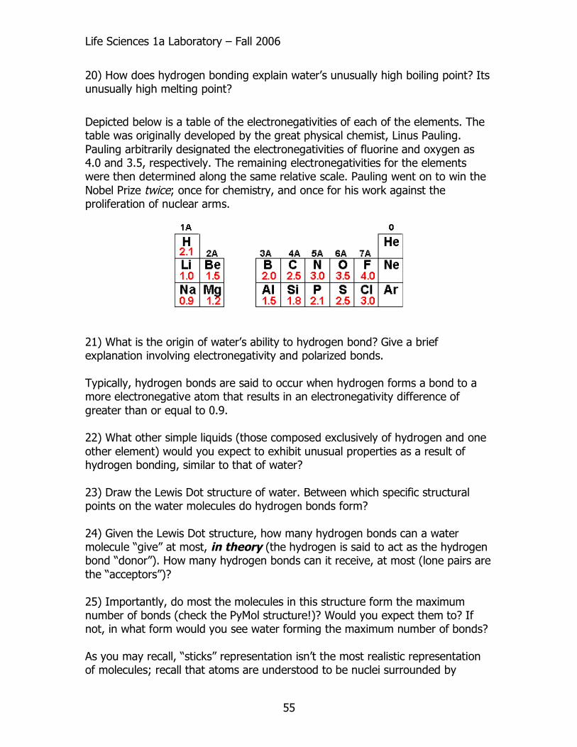
Depicted below is a table of the electronegativities of each of the elements. The table was originally developed by the great physical chemist, Linus Pauling. Pauling arbitrarily designated the electronegativities of fluorine and oxygen as 4.0 and 3.5, respectively. The remaining electronegativities for the elements were then determined along the same relative scale. Pauling went on to win the Nobel Prize twice; once for chemistry, and once for his work against the proliferation of nuclear arms.

21) What is the origin of water’s ability to hydrogen bond? Give a brief explanation involving electronegativity and polarized bonds. Typically, hydrogen bonds are said to occur when hydrogen forms a bond to a more electronegative atom that results in an electronegativity difference of greater than or equal to 0.9. 22) What other simple liquids (those composed exclusively of hydrogen and one other element) would you expect to exhibit unusual properties as a result of hydrogen bonding, similar to that of water? 23) Draw the Lewis Dot structure of water. Between which specific structural points on the water molecules do hydrogen bonds form? 24) Given the Lewis Dot structure, how many hydrogen bonds can a water molecule “give” at most, in theory (the hydrogen is said to act as the hydrogen bond “donor”). How many hydrogen bonds can it receive, at most (lone pairs are the “acceptors”)? 25) Importantly, do most the molecules in this structure form the maximum number of bonds (check the PyMol structure!)? Would you expect them to? If not, in what form would you see water forming the maximum number of bonds? As you may recall, “sticks” representation isn’t the most realistic representation of molecules; recall that atoms are understood to be nuclei surrounded by


56

“electron clouds.” Thus, it is sometimes helpful to view molecules from a “spheres” representation, to get a better view of how the molecules fit together.

• Turn off “Sticks” and “H_Bonds,” turn on “Spheres” Notice how closely packed in molecules are, from this perspective.

• Turn back on “H_Bonds” In this representation, the molecules are so tightly packed, you can’t even see the hydrogen bonds in the structure! Here, we can see how dense solvents can be! Keep in mind that, in liquid form, the molecules are in constant motion, rotating freely around each other. This “free motion” is associated with the water’s “entropy.” However, when water encounters a hydrophobic surface, the water quickly forms a rigid “ice-like” structure that maximizes bonding (increasing enthalpy), but decreases the ability of the water molecules to move, thus decreasing the entropy. Thus, the “hydrophobic effect” is an entropically-driven feature of water; the aggregation of hydrophobic surfaces liberate more water molecules, thus favorably increasing the entropy of the system. Of course, this occurs with a loss of enthalpy, resulting from the break up of the “ice” like lattices.

lab 2: modern legos and tinkertoys - harvard universitysites.fas.harvard.edu/~lsci1a/lab2.pdf ·...

Documents