lab 10 fr3131-5131 - paul bolstad buffering.… · web viewlesson 9: buffering and overlay in...

GIS Fundamentals Lesson 9: Buffering and Overlay

Lesson 9: Buffering and Overlay in ArcGIS - ArcMAP

What You’ll Learn: to apply the concepts of buffering and overlay, two common cartographic operations. You should read chapter 9 in the GIS Fundamentals textbook.

Data: All data are in \L9 subdirectory, including lakes.shp, roads.shp, and public lands in public_Hugo.shp. All distance units are meters.

What You’ll Produce: Three maps, 1) map of lake variable distance buffer zones, 2) map of suitable recreation areas, and 3) map of suitable recreation areas on private land only.

Part One: Buffer ZonesBuffering and overlay are two of the most common operations in cartographic modeling. A buffer zone is an area that is within a given distance from a map feature. Points, lines, or polygons can be buffered. Buffers are used to identify areas surrounding geographic features. For example, you may wish to keep septic systems over 100 meters away from streams, locate housing within a quarter mile of existing roads, keep hiking trails away from seasonally flooded rivers, or make sure most of your city is within some maximum distance from a fire station or school.

When you buffer on a set of features, the output is a set of polygons. (Buffering points or lines creates a new polygon layer). These polygons define an inside region, an area less than the specified buffer distance from the features of interest (e.g., less than 300 meters from a stream), and an outside region, an area more than the specified buffer distance from the features of interest.

These inside and outside regions are typically distinguished by different codes in an attribute table. You should know the specific codes assigned for the software system you use.

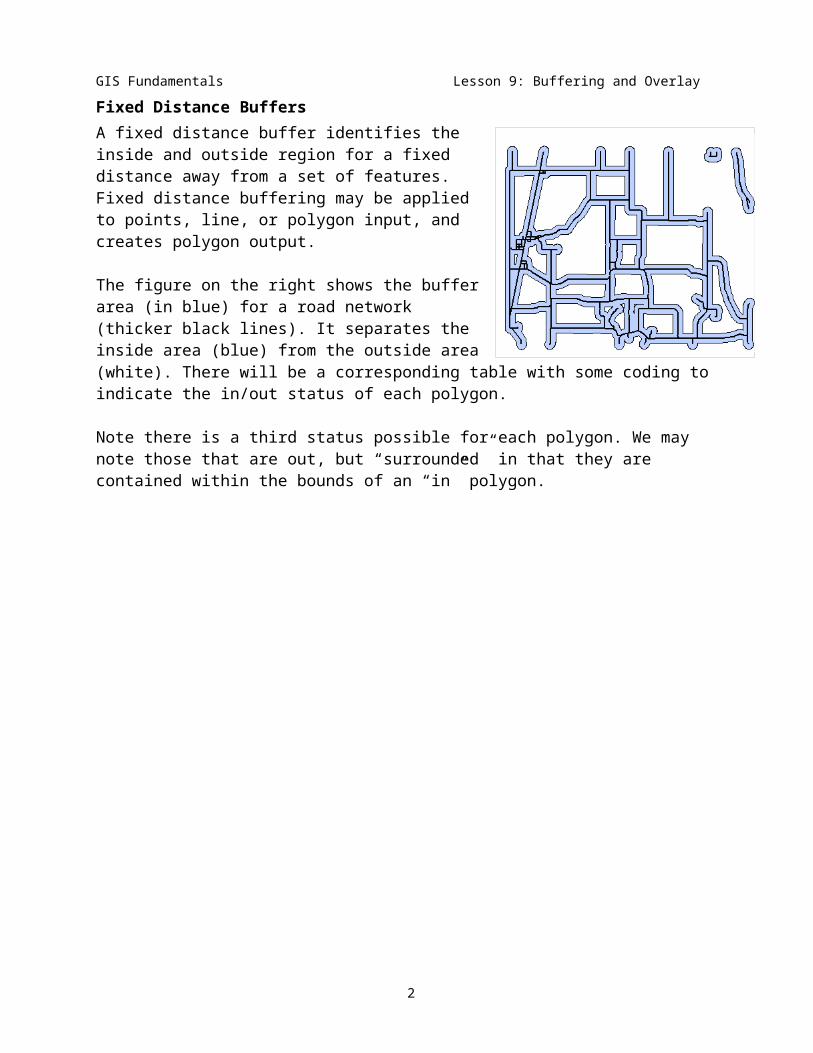
Fixed Distance BuffersA fixed distance buffer identifies the inside and outside region for a fixed distance away from a set of features. Fixed distance buffering may be applied to points, line, or polygon input, and creates polygon output.

The figure on the right shows the buffer area (in blue) for a road network (thicker black lines). It separates the inside area (blue) from the outside area (white). There will be a corresponding table with some coding to indicate the in/out status of each polygon.

Note there is a third status possible for each polygon. We may note those that are out, but “surrounded” in that they are contained within the bounds of an “in” polygon.

1

1

2

3

This item, named dist here, is used to specify the buffer distance.


Variable BuffersAnother variation on buffering will change the buffer distance depending on feature attributes (see the figure, below).

A GIS project may require buffering those lakes to map a minimum distance from shore for installing septic systems. However, the acceptable distance for septic systems may depend on lake size. A large lake could have a system within 100 meters of lakeshore, but a small lake needs a setback of 25 meters.

A variable distance buffer could buffer the lakes coverage by using an attribute that specifies the size class. Different sized buffers would be applied to each lake depending on the size class attribute.

You will create a variable distance buffer in this lab, with the buffer distance defined by lake size.

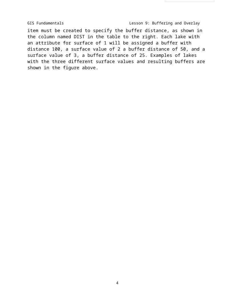
Variable distance buffering requires some way of specifying the distance. This is most often done with an attribute in a table. The buffering operation uses the table entry to determine buffer distance around a feature. A numeric data item must be created to specify the buffer distance, as shown in the column named DIST in the table to the right. Each lake with an attribute for surface of 1 will be assigned a buffer with distance 100, a surface value of 2 a buffer distance of 50, and a surface value of 3, a buffer distance of 25. Examples of lakes with the three different surface values and resulting buffers are shown in the figure above.

2


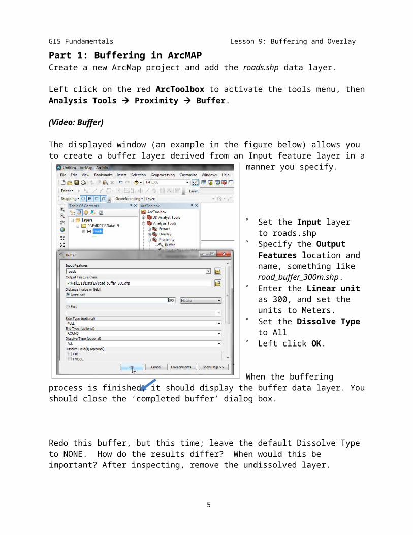
Part 1: Buffering in ArcMAPCreate a new ArcMap project and add the roads.shp data layer.

Left click on the red ArcToolbox to activate the tools menu, then Analysis Tools Proximity Buffer.

(Video: Buffer)

The displayed window (an example in the figure below) allows you to create a buffer layer derived from an Input feature layer in a manner you specify.

Set the Input layer to roads.shp

Specify the Output Features location and name, something like road_buffer_300m.shp.

Enter the Linear unit as 300, and set the units to Meters.

Set the Dissolve Type to All Left click OK.

When the buffering process is finished, it should display the buffer data layer. You should close the ‘completed buffer’ dialog box.

Redo this buffer, but this time; leave the default Dissolve Type to NONE. How do the results differ? When would this be important? After inspecting, remove the undissolved layer.

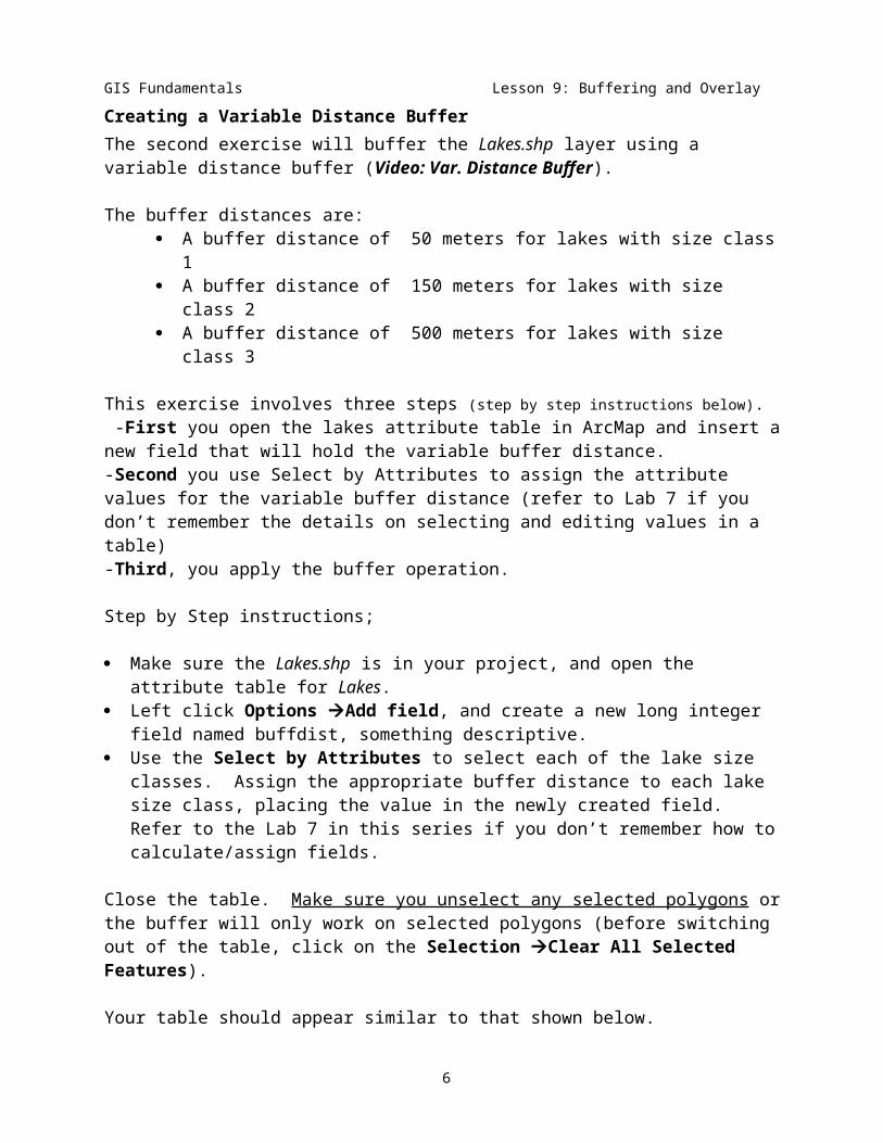
Creating a Variable Distance BufferThe second exercise will buffer the Lakes.shp layer using a variable distance buffer (Video: Var. Distance Buffer).

The buffer distances are: A buffer distance of 50 meters for lakes with size class 1 A buffer distance of 150 meters for lakes with size class 2 A buffer distance of 500 meters for lakes with size class 3

3


This exercise involves three steps (step by step instructions below). -First you open the lakes attribute table in ArcMap and insert a new field that will hold the variable buffer distance.-Second you use Select by Attributes to assign the attribute values for the variable buffer distance (refer to Lab 7 if you don’t remember the details on selecting and editing values in a table)-Third, you apply the buffer operation.

Step by Step instructions;

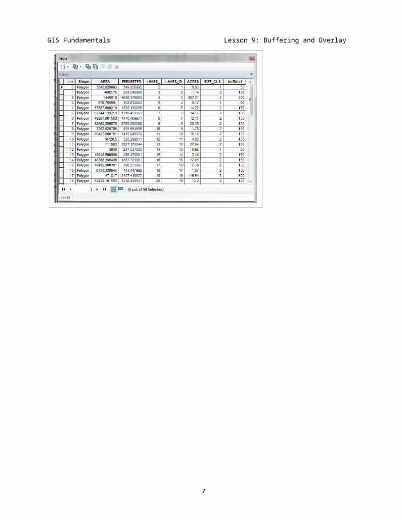
Make sure the Lakes.shp is in your project, and open the attribute table for Lakes. Left click Options Add field, and create a new long integer field named buffdist,

something descriptive. Use the Select by Attributes to select each of the lake size classes. Assign the

appropriate buffer distance to each lake size class, placing the value in the newly created field. Refer to the Lab 7 in this series if you don’t remember how to calculate/assign fields.

Close the table. Make sure you unselect any selected polygons or the buffer will only work on selected polygons (before switching out of the table, click on the Selection Clear All Selected Features).

Your table should appear similar to that shown below.

4


Now create the variable distance buffer:

Left click in the ArcToolbox Analysis Tools Proximity Buffer.

Make sure the Lakes.shp layer is Input.

Name the Output Features something logical, such as Var_Lake_Buffer.shp.

Select the Field (not Distance Unit) radio button.

Specify the field you created in the previous step, buffdist.

Select Dissolve Type as ALL.

When the buffering process is finished, it should display the buffer data layer, close the ‘completed buffer’ dialog box.

Arrange the roads, dissolved fixed distance road buffer, lakes, and dissolved variable distance lake buffer layers so that you can see all three, as in the figure below.

Create and print/export a layout with the roads, lakes, and their buffers, as in the view shown here. Make sure the order is as shown here, so you may see most of each layer. The order is, from the top, 1) roads, 2) road buffer, 3) lakes, 4) lake buffer.

Your data view should look something like the figure at right.

Create a layout, and label each layer with descriptive text in the TOC/legend, and include a scale bar, north arrow, and title.

5


Part Two: Overlay in ArcMAPOverlays are another common cartographic modeling operation. An overlay is the primary way to combine information from two separate themes. Overlays are most common for polygonal data, and perform a geometric intersection, which results in a new layer with the combined attributes of both initial layers.

Our goal in this exercise is to find potential campgrounds sites for a State Park. The campground needs to be within the buffer zone created for the lakes. However, these will be ‘drive in’ sites and they must also be within the buffer zone of the roads. The final map will show locations that are both within 50, 150 or 500 meters of a lake (depending on the size of the lake) and within 300 meters of a road. We have already created our starting Layers. These are the variable distance lakes buffer, and the fixed distance roads buffer from the previous exercise.

In ArcMap we must modify input layers prior to overlay so that we may easily interpret the results after overlay. We add a field to each input data layer that specifies the factors we wish to use later in our analysis.

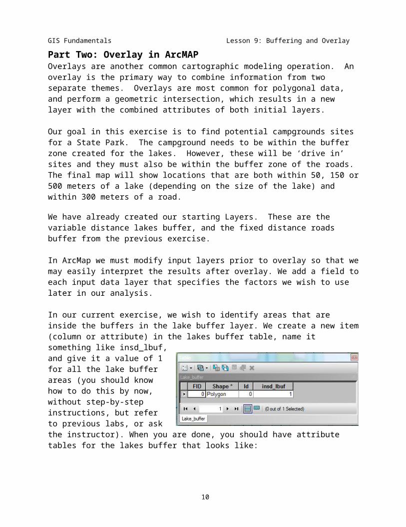
In our current exercise, we wish to identify areas that are inside the buffers in the lake buffer layer. We create a new item (column or attribute) in the lakes buffer table, name it something like insd_lbuf, and give it a value of 1 for all the lake buffer areas (you should know how to do this by now, without step-by-step instructions, but refer to previous labs, or ask the instructor). When you are done, you should have attribute tables for the lakes buffer that looks like:

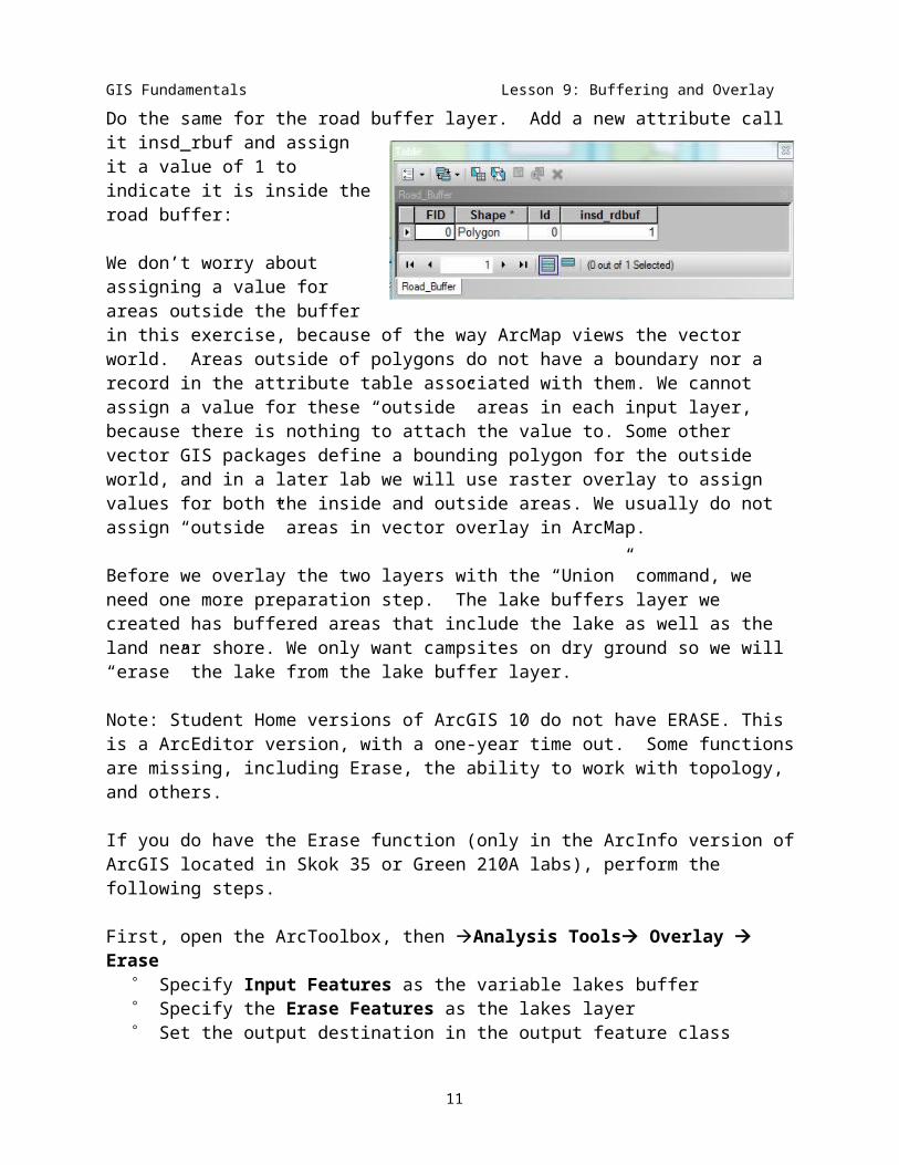
Do the same for the road buffer layer. Add a new attribute call it insd_rbuf and assign it a value of 1 to indicate it is inside the road buffer:

We don’t worry about assigning a value for areas outside the buffer in this exercise, because of the way ArcMap views the vector world. Areas outside of polygons do not have a boundary nor a record in the attribute table associated with them. We cannot assign a value for these “outside” areas in each input layer, because there is nothing to attach the value to. Some other vector GIS packages define a bounding polygon for the outside world, and in a later lab we will use raster overlay to assign values for both the inside and outside areas. We usually do not assign “outside” areas in vector overlay in ArcMap.

6


Before we overlay the two layers with the “Union” command, we need one more preparation step. The lake buffers layer we created has buffered areas that include the lake as well as the land near shore. We only want campsites on dry ground so we will “erase” the lake from the lake buffer layer.

Note: Student Home versions of ArcGIS 10 do not have ERASE. This is a ArcEditor version, with a one-year time out. Some functions are missing, including Erase, the ability to work with topology, and others.

If you do have the Erase function (only in the ArcInfo version of ArcGIS located in Skok 35 or Green 210A labs), perform the following steps.

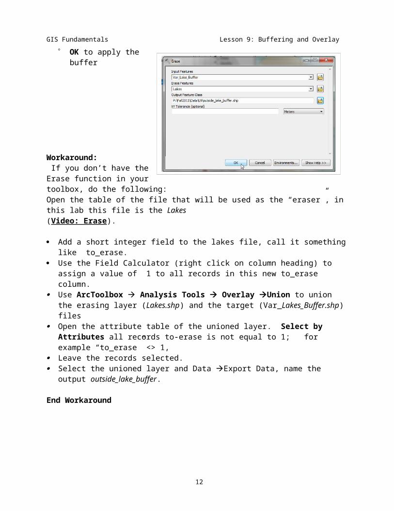
First, open the ArcToolbox, then Analysis Tools Overlay Erase Specify Input Features as the variable lakes buffer Specify the Erase Features as the lakes layer Set the output destination in the output feature class OK to apply the buffer

Workaround: If you don’t have the Erase function in your toolbox, do the following:Open the table of the file that will be used as the “eraser”, in this lab this file is the Lakes (Video: Erase).

Add a short integer field to the lakes file, call it something like to_erase. Use the Field Calculator (right click on column heading) to assign a value of 1 to all

records in this new to_erase column. Use ArcToolbox Analysis Tools Overlay Union to union the erasing layer

(Lakes.shp) and the target (Var_Lakes_Buffer.shp) files Open the attribute table of the unioned layer. Select by Attributes all records to-

erase is not equal to 1; for example “to_erase” <> 1, Leave the records selected. Select the unioned layer and Data Export Data, name the output

outside_lake_buffer.

End Workaround

7


The final step is to overlay the two buffer layers (Video: Union). Select ArcToolbox Analysis Tools Overlay Union Specify the input layers – outside_lake_buffer and road_buffer_300m. Specify the output layer Union_Lk_Rd. Press OK.

Examine the “unioned” layer and open the attribute table for this layer. Select the polygons that meet both the within the roads buffer and the within the lakes buffer criteria (see the figure below for some hints).

Note the number of records selected.

Why do you have only 3 records? You can see more polygons on the screen.

ArcMap groups polygons in the data files when performing analysis. When we are finished with our analysis we will “ungroup” polygons in the file, creating a table row for each polygon.

Open the attribute table for the roadbuffer outside Lake buffer union, and create a new field named something like in_both to identify those areas that meet both the inside road buffer and inside lake buffer criteria (refer to previous exercises).

Use Select by Attributes to find those areas with insd_lbuf=1 and insd_rbuf = 1, and assign them the number 1 using the Field Calculator (previous exercises, or see graphic below).

8


Close the attribute table, make sure the Union_Lk_Rd layer is selected and right click on the layer name in the TOC. Right click on the Union_Lk_Rd layer in the table of contents, and select Data Export Data and export only the selected (where in_both =1) to a file called Acceptable_Areas.

9


Select Toolbox Data Base Management Features Multipart to Singlepart. (Video: Multipart). This will ungroup the combined polygons to and create a table row for each. You should have 32 records in the table for the singlepart file.

Display the roads, singlepart acceptable areas, and lakes in the view. It should look something like the figure at right.

Now before you print/export the map you need to determine the size (in acres or hectares) of your acceptable sites. (Video: Area).

Open the attribute table and add a float or double field named “Hectares” with a precision of at least 12, scale of 1 or 2. Verify that there are 32 records in the table.

Right click on the column heading for the Hectares column, and left click on Calculate Geometry in the dropdown menu.

Specify Area in the Property drop down box, the default coordinate system, and Hectares, then O.K.:

The new Hectares column should be populated with numbers, with values between 0 and 300.

Right click on the Hectares column, and then left click on Statistics: This should display a set of summary statistics.

Count should be 32. If it isn’t, perhaps you selected the wrong layer, or made a mistake in the processing chain.

The total area should be over 1000, but below 1200. If it is way off, perhaps you selected incorrect units in calculating geometry.

10


Create a second .pdf as suggested below:

11


PART 3 Estimate the amount of Private (non-public) land in your proposed Campsites locations.

Create a new project or data frame, and add the layers roads.shp, Lakes.shp, acceptable areas.shp, and Public_Hugo.shp (see figure below).

Open the ArcToolbox, then Analysis Overlay Erase

Remember, if you have the ArcMap Student (or ArcView) edition, you do not have the Erase tool, and should use the Workaround described earlier.

From the acceptable areas layer, use the Public_Hugo as the Erase Features Layer. This removes the publicly owned land in Hugo from your Acceptable Areas.

Name you new layer; in the Output Feature Class to ‘Campgrounds_on_Private_Land’. This is the land that would need to be acquired if the community wants to build campsites.

Recalculate the area of Campground_on_Private Land and note it size in hectares. Subtract it from your previous area calculation (the total Acceptable Areas from Part 2).

Create a Layout that includes roads, lakes, and Campgrounds on Private Land. (see below).

12


Label each layer with descriptive text in the legend, and include a scale bar, north arrow, and title.

Make sure you add the area measurement of the suitable for campground on private land, in hectares.

Print or Export a map from this layout, your third and final map for this lesson.

13

lab 10 fr3131-5131 - paul bolstad buffering.… · web viewlesson 9: buffering and overlay in...

Documents