1

LAB 1 – The Scientific Method

Objectives

1. Apply the basic principles of the scientific method. 2. Generate testable hypotheses. 3. Identify the components of an experiment. 4. Design an experiment. 5. Graph experimental results.

Lab Safety Before you begin this laboratory it is essential that we address lab safety. You first will watch a brief video on the importance of laboratory safety which will also introduce you to various safety items in the laboratory (e.g., fire extinguisher, eyewash, broken glass disposal). Your instructor will then review the Lab Safety Rules (a copy of which can be found at the beginning of the lab manual) which must be followed throughout this course for your own safety and the safety of others.

Part 1: The Scientific Method

The field of science is based on observation and measurement. If a scientist cannot observe and measure something that can be described and repeated by others, then it is not considered to be objective and scientific. In general, the scientific method is a process composed of several steps:

1. observation – a certain pattern or phenomenon of interest is observed which leads to a question such as “What could explain this observation?”

2. hypothesis – an educated guess is formulated to explain what might be happening

3. experiment – an experiment or study is carefully designed to test the hypothesis, and the resulting data are presented in an appropriate form

4. conclusion – the data is concluded to “support” or “not support” the hypothesis To illustrate the scientific method, let’s consider the following observation:

A scientist observes that the addition of Compound X appears to increase plant growth, which leads to the question: “Does the addition of Compound X really increase plant growth?”

2

Hypotheses

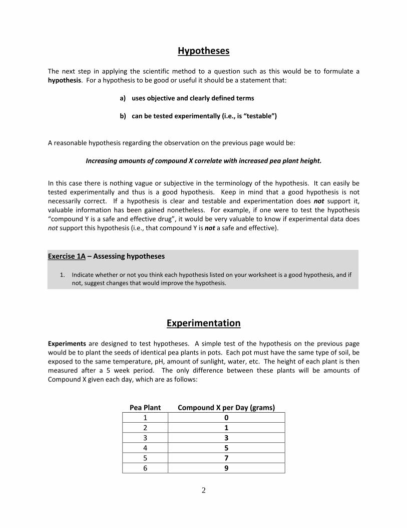
The next step in applying the scientific method to a question such as this would be to formulate a hypothesis. For a hypothesis to be good or useful it should be a statement that:

a) uses objective and clearly defined terms

b) can be tested experimentally (i.e., is “testable”) A reasonable hypothesis regarding the observation on the previous page would be:

Increasing amounts of compound X correlate with increased pea plant height.

In this case there is nothing vague or subjective in the terminology of the hypothesis. It can easily be tested experimentally and thus is a good hypothesis. Keep in mind that a good hypothesis is not necessarily correct. If a hypothesis is clear and testable and experimentation does not support it, valuable information has been gained nonetheless. For example, if one were to test the hypothesis “compound Y is a safe and effective drug”, it would be very valuable to know if experimental data does not support this hypothesis (i.e., that compound Y is not a safe and effective). Exercise 1A – Assessing hypotheses

1. Indicate whether or not you think each hypothesis listed on your worksheet is a good hypothesis, and if not, suggest changes that would improve the hypothesis.

Experimentation

Experiments are designed to test hypotheses. A simple test of the hypothesis on the previous page would be to plant the seeds of identical pea plants in pots. Each pot must have the same type of soil, be exposed to the same temperature, pH, amount of sunlight, water, etc. The height of each plant is then measured after a 5 week period. The only difference between these plants will be amounts of Compound X given each day, which are as follows:

Pea Plant Compound X per Day (grams) 1 0 2 1 3 3 4 5 5 7 6 9

3

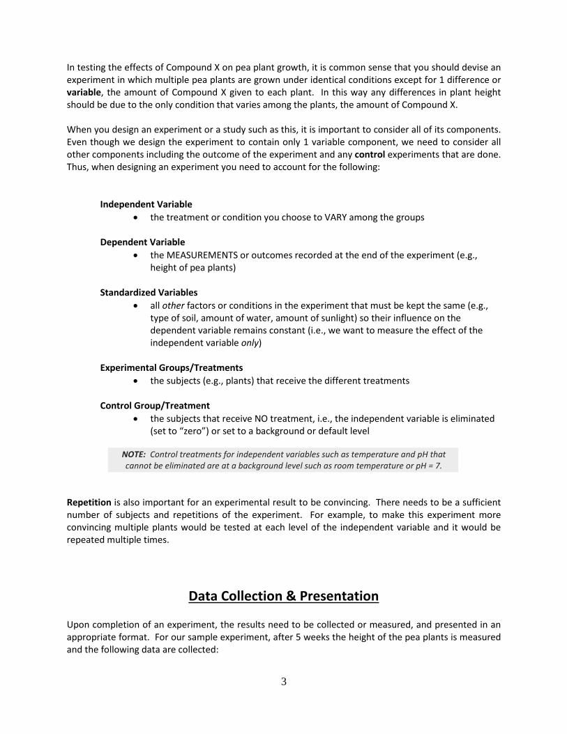
In testing the effects of Compound X on pea plant growth, it is common sense that you should devise an experiment in which multiple pea plants are grown under identical conditions except for 1 difference or variable, the amount of Compound X given to each plant. In this way any differences in plant height should be due to the only condition that varies among the plants, the amount of Compound X. When you design an experiment or a study such as this, it is important to consider all of its components. Even though we design the experiment to contain only 1 variable component, we need to consider all other components including the outcome of the experiment and any control experiments that are done. Thus, when designing an experiment you need to account for the following:

Independent Variable • the treatment or condition you choose to VARY among the groups

Dependent Variable

• the MEASUREMENTS or outcomes recorded at the end of the experiment (e.g., height of pea plants)

Standardized Variables

• all other factors or conditions in the experiment that must be kept the same (e.g., type of soil, amount of water, amount of sunlight) so their influence on the dependent variable remains constant (i.e., we want to measure the effect of the independent variable only)

Experimental Groups/Treatments

• the subjects (e.g., plants) that receive the different treatments

Control Group/Treatment • the subjects that receive NO treatment, i.e., the independent variable is eliminated

(set to “zero”) or set to a background or default level

NOTE: Control treatments for independent variables such as temperature and pH that cannot be eliminated are at a background level such as room temperature or pH = 7.

Repetition is also important for an experimental result to be convincing. There needs to be a sufficient number of subjects and repetitions of the experiment. For example, to make this experiment more convincing multiple plants would be tested at each level of the independent variable and it would be repeated multiple times.

Data Collection & Presentation Upon completion of an experiment, the results need to be collected or measured, and presented in an appropriate format. For our sample experiment, after 5 weeks the height of the pea plants is measured and the following data are collected:

4

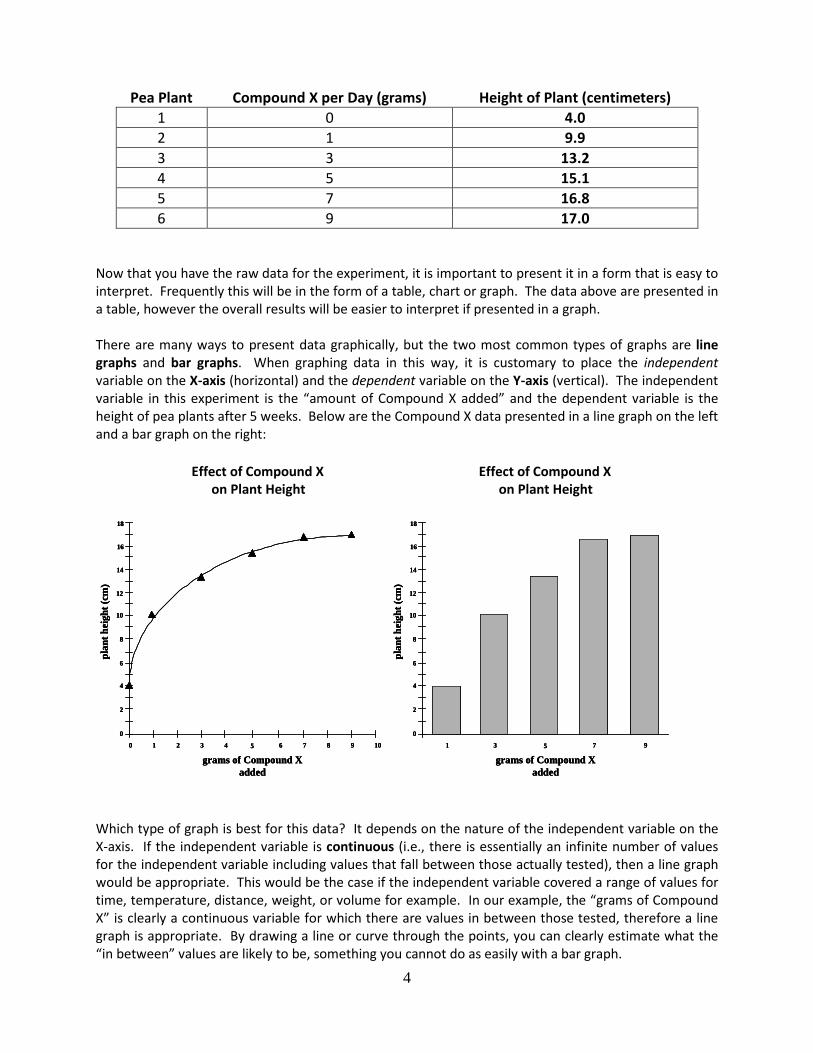
Pea Plant Compound X per Day (grams) Height of Plant (centimeters) 1 0 4.0 2 1 9.9 3 3 13.2 4 5 15.1 5 7 16.8 6 9 17.0

Now that you have the raw data for the experiment, it is important to present it in a form that is easy to interpret. Frequently this will be in the form of a table, chart or graph. The data above are presented in a table, however the overall results will be easier to interpret if presented in a graph. There are many ways to present data graphically, but the two most common types of graphs are line graphs and bar graphs. When graphing data in this way, it is customary to place the independent variable on the X-axis (horizontal) and the dependent variable on the Y-axis (vertical). The independent variable in this experiment is the “amount of Compound X added” and the dependent variable is the height of pea plants after 5 weeks. Below are the Compound X data presented in a line graph on the left and a bar graph on the right: Effect of Compound X Effect of Compound X on Plant Height on Plant Height

Which type of graph is best for this data? It depends on the nature of the independent variable on the X-axis. If the independent variable is continuous (i.e., there is essentially an infinite number of values for the independent variable including values that fall between those actually tested), then a line graph would be appropriate. This would be the case if the independent variable covered a range of values for time, temperature, distance, weight, or volume for example. In our example, the “grams of Compound X” is clearly a continuous variable for which there are values in between those tested, therefore a line graph is appropriate. By drawing a line or curve through the points, you can clearly estimate what the “in between” values are likely to be, something you cannot do as easily with a bar graph.

14

6

0

2

4

8

10

12

5 6 7 8 9 101 2 3 40

plan

t hei

ght (

cm)

grams of Compound Xadded

16

18

14

6

0

2

4

8

10

12

5 7 91 3

plan

t hei

ght (

cm)

grams of Compound Xadded

16

18

14

6

0

2

4

8

10

12

5 6 7 8 9 101 2 3 40

plan

t hei

ght (

cm)

grams of Compound Xadded

16

18

14

6

0

2

4

8

10

12

5 6 7 8 9 101 2 3 40

plan

t hei

ght (

cm)

grams of Compound Xadded

16

18

14

6

0

2

4

8

10

12

5 7 91 3

plan

t hei

ght (

cm)

grams of Compound Xadded

16

18

14

6

0

2

4

8

10

12

5 7 91 3

plan

t hei

ght (

cm)

grams of Compound Xadded

16

18

5

If the independent variable is discontinuous or discrete (i.e., there are very limited or finite values for the independent variable), then a bar graph would be appropriate. For example, if you wanted to graph the average GPA of students at each of the nine LACCD community colleges, the independent variable would be the specific school (the dependent variable would be the average GPA). There are only nine possible “values” for the independent variable, so in this case a bar graph would be most appropriate. When you’re ready to create a graph, you need to determine the range of values for each axis and to scale and label each axis properly. It is also important to give your graph a title. Notice that the range of values on each axis of these graphs is slightly larger than the range of values for each variable. As a result little space is wasted and the graph is well spread out and easy to interpret. It is also essential that the units (e.g., grams or centimeters) for each axis be clearly indicated, and that each interval on the scale represents the same quantity. By scaling each axis regularly and evenly, each value plotted on the graph will be accurately represented in relation to the other values.

Conclusions

Once the data from an experiment are collected and presented, a conclusion is made with regard to the original hypothesis. Based on the graph on the previous page it is clear that all of the plants that received Compound X grew taller than the control plant which received no Compound X. In fact, there is a general trend that increasing amounts of Compound X cause the pea plant to grow taller (except for plants 5 and 6 which are very close). These data clearly support the hypothesis, but they by no means prove it. In reality, you can never prove that a hypothesis is correct, you can only accumulate experimental data that support it. However if you consistently produce experimental data that do not support a hypothesis, you should discard it and come up with a new hypothesis to test. Exercise 1B – Effect of distance on shooting accuracy In this exercise, you will design an experiment to determine the effect of distance on the accuracy of shooting paper balls into a beaker (and also determine which person in your group is the best shot!). Each student will attempt to throw small paper balls into a large beaker at 3 different distances in addition to the control (which should be 0 cm, i.e., a slam dunk!). You will measure each distance using the metric system and determine how many attempts are made out of 10 total attempts at each distance.

1. State your hypothesis and identify your independent and dependent variables.

2. Place the large beaker on your lab table at each test distance and record how many attempts out of 10 you make.

3. Graph the data for each member of your group on a single graph (use different curves for each person)

and answer the corresponding questions on your worksheet.

4. Conclude whether or not the data support your hypothesis and answer the associated questions on your worksheet.

6

Exercise 1C – Graphing practice

1. On your worksheet, use the grids provided to graph the three sets of data provided. As you do so, refer to the previous section to ensure you set up and label your graphs properly.

NOTE: Your instructor may ask you to do this on your own time in which case you should move on to the next section.

Designing an Experiment

In the final exercise for this lab you will work together with the members of your group to apply all the principles you have just learned to come up with a hypothesis and design an experiment to test this hypothesis. Let’s go through an example just to make sure everything is clear. Let’s assume your group is interested in the following question:

Does a car get better gas mileage with the windows open or the windows closed? Based on this question your group would come up with a testable hypothesis such as the following:

Cars get better gas mileage with the windows closed than with the windows open. Your group would then plan an experiment to test this hypothesis. As you did so you would realize that such an experiment is not so straightforward. There are many different types of cars (sedans, vans, pickups, SUVs) and they may not all give the same result. Plus some cars have 4 adjustable windows and others only 2, and windows can be partially open as well. To keep the experiment simple you might choose to test one type of car that seems “typical” such as a 4-door sedan, and you might limit the windows to being completely open or completely closed. Based on this you might plan an experiment such as this:

1) Fill the gas tank of the 4-door sedan to be tested and drive it on a 100 mile circular route with all the windows closed.

2) Once the route is complete, fill the gas tank to determine the amount of gas burned and divide by the miles traveled on the route to calculate the gas mileage with the windows closed.

3) Repeat the experiment with the same car under the same conditions (i.e., same driver, traffic conditions, etc) with all 4 windows completely open.

4) Compare the gas mileage in each case to see if your hypothesis is supported.

Before doing the experiment you would analyze the experimental plan to make sure it contains all the necessary components: Dependent Variable

• the gas mileage (i.e., miles per gallon or MPG) One Independent Variable

• the state of the car’s windows – open or closed

7

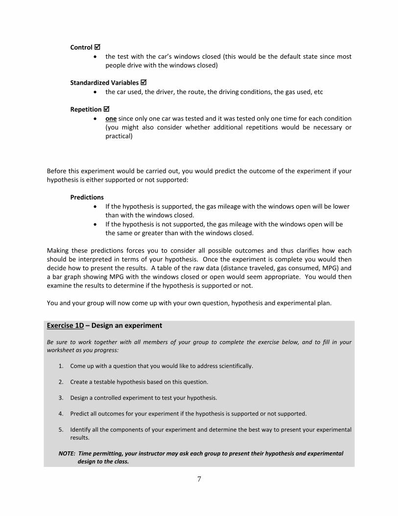
Control • the test with the car’s windows closed (this would be the default state since most

people drive with the windows closed)

Standardized Variables • the car used, the driver, the route, the driving conditions, the gas used, etc

Repetition

• one since only one car was tested and it was tested only one time for each condition (you might also consider whether additional repetitions would be necessary or practical)

Before this experiment would be carried out, you would predict the outcome of the experiment if your hypothesis is either supported or not supported: Predictions

• If the hypothesis is supported, the gas mileage with the windows open will be lower than with the windows closed.

• If the hypothesis is not supported, the gas mileage with the windows open will be the same or greater than with the windows closed.

Making these predictions forces you to consider all possible outcomes and thus clarifies how each should be interpreted in terms of your hypothesis. Once the experiment is complete you would then decide how to present the results. A table of the raw data (distance traveled, gas consumed, MPG) and a bar graph showing MPG with the windows closed or open would seem appropriate. You would then examine the results to determine if the hypothesis is supported or not. You and your group will now come up with your own question, hypothesis and experimental plan.

Exercise 1D – Design an experiment Be sure to work together with all members of your group to complete the exercise below, and to fill in your worksheet as you progress:

1. Come up with a question that you would like to address scientifically.

2. Create a testable hypothesis based on this question.

3. Design a controlled experiment to test your hypothesis.

4. Predict all outcomes for your experiment if the hypothesis is supported or not supported.

5. Identify all the components of your experiment and determine the best way to present your experimental results.

NOTE: Time permitting, your instructor may ask each group to present their hypothesis and experimental

design to the class.

8

Before you leave, please make sure your table is clean, organized, and contains all supplies listed below so that the next lab will be ready to begin. Thank you!

Supply List

• 1000 ml Beaker

• Metric Ruler

• Newspaper for making balls (do not use paper towels for the balls!)

9

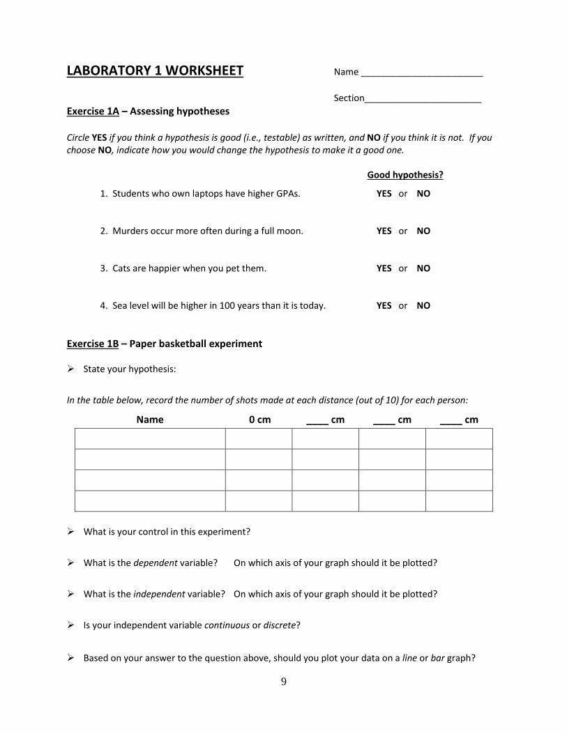
LABORATORY 1 WORKSHEET Name ________________________ Section_______________________ Exercise 1A – Assessing hypotheses Circle YES if you think a hypothesis is good (i.e., testable) as written, and NO if you think it is not. If you choose NO, indicate how you would change the hypothesis to make it a good one. Good hypothesis?

1. Students who own laptops have higher GPAs. YES or NO

2. Murders occur more often during a full moon. YES or NO

3. Cats are happier when you pet them. YES or NO

4. Sea level will be higher in 100 years than it is today. YES or NO

Exercise 1B – Paper basketball experiment State your hypothesis:

In the table below, record the number of shots made at each distance (out of 10) for each person:

Name 0 cm ____ cm ____ cm ____ cm

What is your control in this experiment?

What is the dependent variable? On which axis of your graph should it be plotted?

What is the independent variable? On which axis of your graph should it be plotted?

Is your independent variable continuous or discrete?

Based on your answer to the question above, should you plot your data on a line or bar graph?

10

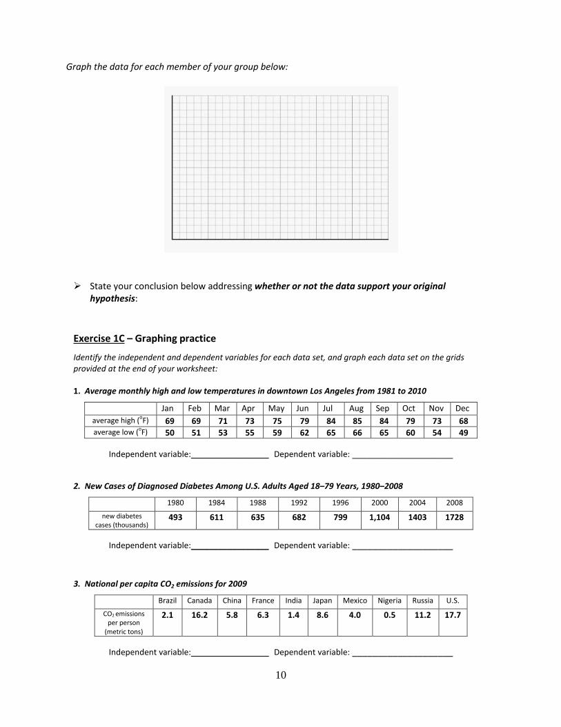
Graph the data for each member of your group below:

State your conclusion below addressing whether or not the data support your original

hypothesis: Exercise 1C – Graphing practice

Identify the independent and dependent variables for each data set, and graph each data set on the grids provided at the end of your worksheet: 1. Average monthly high and low temperatures in downtown Los Angeles from 1981 to 2010

Jan Feb Mar Apr May Jun Jul Aug Sep Oct Nov Dec average high (oF) 69 69 71 73 75 79 84 85 84 79 73 68 average low (oF) 50 51 53 55 59 62 65 66 65 60 54 49

Independent variable:_________________ Dependent variable: ____________________

2. New Cases of Diagnosed Diabetes Among U.S. Adults Aged 18–79 Years, 1980–2008

1980 1984 1988 1992 1996 2000 2004 2008

new diabetes cases (thousands)

493 611 635 682 799 1,104 1403 1728

Independent variable:_________________ Dependent variable: ____________________

3. National per capita CO2 emissions for 2009

Brazil Canada China France India Japan Mexico Nigeria Russia U.S. CO2 emissions

per person (metric tons)

2.1 16.2 5.8 6.3 1.4 8.6 4.0 0.5 11.2 17.7

Independent variable:_________________ Dependent variable: ____________________

11

Exercise 1D – Design an experiment

Write the question your group has chosen to address scientifically below: State your hypothesis based on the question above: Outline your experimental plan to test this hypothesis: Identify the following components of your experimental plan: Dependent Variable – Independent Variable – Control – Standardized Variables – Repetition – Predict the possible outcomes of your experiment by completing the following sentences: If the hypothesis is supported… If the hypothesis is not supported… Indicate below how you would present your experimental results (e.g., type of graph):

12

13

14

15

16

17

18