lab 1 interfacing with other programming languages … · lab 1 interfacing with other programming...
TRANSCRIPT

Lab 1
Interfacing With OtherProgramming LanguagesUsing Cython
Lab Objective: Learn to interface with object files using Cython. This lab should
be worked through on a machine that has already been configured to build Cython
extensions using gcc or MinGW.
Suppose you are writing a program in Python, but would like to call code written
in another language. Perhaps this code has already been debugged and heavily
optimized, so you do not want to simply re-implement the algorithm in Python or
Cython. In technical terms, you want Python to interface (or communicate) with
the other language. For example, NumPy’s linear algebra functions call functions
from LAPACK and BLAS, which are written in Fortran.
One way to have Python interface with C is to write a Cython wrapper for the
C function. The wrapper is a Cython function that calls the C function. This is
relatively easy to do because Cython compiles to C. From Python, you can call the
wrapper, which calls the C function (see Figure TODO). In this lab you will learn
how to use Cython to wrap a C function.
Wrapping with Cython: An Overview
When you use Cython to wrap a C function, you just write a Cython function that
calls the C function. To actually do this, we need to understand a little bit more
about how C works.
After you write a program in C, you pass it to a compiler. The compiler turns
your C code into machine code, i.e., instructions that your computer can read. The
output of the compiler is an object file.
In our scenario, we have C code defining a single function that we would like
to wrap in Cython. This C code has already been compiled to an object file. The
protocol for calling the C code from Cython is similar to calling it from C:
1. we need to include a header file for the C code in our Cython code, and
2. we must link to the object file compiled from the C code when we compile the
Cython code.
1

2 Lab 1. Interfacing With Other Programming Languages Using Cython
ctridiag.hdeclare ctridiag()
ctridiag.cdefine ctridiag()
COMPILE
ctridiag.oobject file callable
from C
cython ctridiag.pyxdefine cytridiag()
COMPILE
ctridiag.soobject file callable
from Python
INCLUDE
LINK
Figure 1.1: This diagram shows the relationships between the files used to write
a Cython wrapper for ctridiag(). In fact, the Cython file cython ctridiag.pyx
compiles first to C code and then to the shared object file, but we have omitted this
step from the diagram.
A header for a file contains the declaration of the function defined in the file.
We include the header in the Cython code so that the compiler can check that
the function is called with the right number and types of arguments. Then, when
we tell the compiler to link to the object file, we simply tell it where to find the
instructions defining the function declared in the header.
The Cython code will compile to a second object file. This object file defines a
module that can be imported into Python. See Figure 1.1.
Wrapping with Cython: An Example
As an example, we will wrap the C function ctridiag() below. This function
computes the solution to a tridiagonal system Av = x. Its parameters are pointers
to four 1-D arrays, which satisfy the following:
• Arrays a and c have length n-1 and contain the first subdiagonal and super-
diagonal of A, respectively.
• Arrays b and x have length n and represent the main diagonal of A and x,
respectively.
The array c is used to store temporary values and x is transformed into the solution
of the system.
1 void ctridiag(double *a, double *b, double *c, double *x, int n){

3
2 // Solve a tridiagonal system inplace.
// Initialize temporary variable and index.
4 int i;
double temp;
6 // Perform necessary computation in place.
// Initial steps
8 c[0] = c[0] / b[0];
x[0] = x[0] / b[0];
10 // Iterate down arrays.
for (i=0; i<n-2; i++){
12 temp = 1.0 / (b[i+1] - a[i] * c[i]);
c[i+1] = c[i+1] * temp;
14 x[i+1] = (x[i+1] - a[i] * x[i]) * temp;
}
16 // Perform last step.
x[n-1] = (x[n-1] - a[n-2] * x[n-2]) / (b[n-1] - a[n-2] * c[n-2]);
18 // Perform back substitution to finish constructing the solution.
for (i=n-2; i>-1; i--){
20 x[i] = x[i] - c[i] * x[i+1];
}
22 }
ctridiag.c
This terminal command tells the C-compiler gcc to compiles ctridiag.c to an
object file ctridiag.o.
$ gcc -fPIC -c ctridiag.c -o ctridiag.o
The -fPIC option is required because we will later link to this object file when
compiling a shared object file. The -c flag prevents the compiler from raising an
error even though ctridiag.c does not have a main function.
Write a Header For ctridiag.c
The header file essentially contains a function declaration for ctridiag(). It tells
Cython how to use the object file ctridiag.o.
1 extern void ctridiag(double* a, double* b, double* c, double* x, int n);
2 // This declaration specifies what arguments should be passed
// to the function called `ctridiag.'
ctridiag.h
Write a Cython Wrapper
Next we write a Cython file containing a function that “wraps” ctridiag(). This file
must include the header we wrote in the previous step.
1 # Include the ctridiag() function as declared in ctridiag.h
2 # We use a cdef since this function will only be called from Cython
cdef extern from "ctridiag.h":
4 void ctridiag(double* a, double* b, double* c, double* x, int n)
6 # Define a Cython wrapper for ctridiag().

4 Lab 1. Interfacing With Other Programming Languages Using Cython
# Accept four NumPy arrays of doubles
8 # This will not check for out of bounds memory accesses.
cpdef cytridiag(double[:] a, double[:] b, double[:] c, double[:] x):
10 cdef int n = x.size
ctridiag(&a[0], &b[0], &c[0], &x[0], n)
cython ctridiag.pyx
Some comments on this code are in order. First, including the header for ctridiag
() allows us to call this function even though it was not defined in this file. This is
a little like importing NumPy at the start of your Python script.
Second, the arguments of the Cython function cytridiag() are not in bijection
with the arguments of ctridiag(). In fact, Cython does not need to know the size
of the NumPy arrays it accepts as inputs because these arrays are objects that
carry that information with them. We extract this information and pass it to the
C function inside the Cython wrapper.
However, it is possible to unintentionally access memory outside of an array by
calling this function. For example, suppose the input arrays a, b, c, and x are of
sizes 4, 5, 3, and 5. Since x is used to determine the size of the system, the function
ctridiag() will expect c to have length 4. At some point, ctridiag() will likely try
to read or even write to the 4th entry of c. This address does exist in memory,
but it does not contain an entry of c! Therefore, this function must be called by a
responsible user who knows the sizes of her arrays. Alternatively, you could check
the sizes of the arrays in the Cython wrapper before passing them to the C function.
Finally, the C function expects a parameter double* a, meaning that a is a pointer
to (i.e., the address of) a double. The funtion ctridiag() expects this double to be
the first entry of the array a. So instead of passing the object a to ctridiag(), we
find the first entry of a with a[0], and then take its address with the & operator.
Compile the Cython Wrapper
Now we can compile cython ctridiag.pyx to build the Python extension. The
following setup file uses distutils to compile the Cython file, and may be run on
Windows, Linux, or Macintosh-based computers. Notice that in line 28, we link to
the existing object file ctridiag.o.
1 # Import needed setup functions.
2 from distutils.core import setup
from distutils.extension import Extension
4 # This is part of Cython's interface for distutils.
from Cython.Distutils import build_ext
6 # We still need to include the directory
# containing the NumPy headers.
8 from numpy import get_include
# We still need to run one command via command line.
10 from os import system
12 # Compile the .o file we will be accessing.
# This is independent building the Python extension module.
14 shared_obj = "gcc -fPIC -03 -c ctridiag.c -o ctridiag.o"
print shared_obj
16 system(shared_obj)

5
18 # Tell Python how to compile the extension.
ext_modules = [Extension(
20 # Module name:
"cython_ctridiag",
22 # Cython source file:
["cython_ctridiag.pyx"],
24 # Other compile arguments
# This flag doesn't do much this time,
26 # but this is where it would go.
extra_compile_args=["-fPIC", "-O3"],
28 # Extra files to link to:
extra_link_args=["ctridiag.o"])]
30
# Build the extension.
32 setup(name = 'cython_ctridiag',cmdclass = {'build_ext': build_ext},
34 # Include the directory with the NumPy headers when compiling.
include_dirs = [get_include()],
36 ext_modules = ext_modules)
ctridiag setup distutils.py
This setup file can be called from the command line with the following command.
python ctridiag_setup_distutils.py build_ext --inplace
The --inplace flag tells the script to compile the extension in the current directory.
The optional section at the end of this lab contains setup files that build the Python
extension by hand on various operating systems.
Warning
If at any point you need to make a change to the source file (in this case
ctridiag.c) it is wise to delete all files that are generated in the build process
to guarantee you have a clean build.
Test the Python Extension
After running the setup file, you should have a Python module called cython_cytridiag
that defines a function cytridiag(). You can import this module into IPython as
usual. However, if you modify ctridiag() and then try to recompile the extension,
you may get an error if the module is currently in use. Hence, if you are frequently
recompiling your extension, it is wise to test it with a script.
The following script tests the module cython_cytridiag.
1 import numpy as np
2 from cython_ctridiag import cytridiag as ctri
4 def init_tridiag(n):
a = np.random.random_integers(-9,9,n).astype("float")
6 b = np.random.random_integers(-9,9,n).astype("float")
c = np.random.random_integers(-9,9,n).astype("float")
8

6 Lab 1. Interfacing With Other Programming Languages Using Cython
A = np.zeros((b.size,b.size))
10 np.fill_diagonal(A,b)
np.fill_diagonal(A[1:,:-1],a)
12 np.fill_diagonal(A[:-1,1:],c)
return a,b,c,A
14
if __name__ == "__main__":
16 n = 10
a,b,c,A = init_tridiag(n)
18 d = np.random.random_integers(-9,9,n).astype("float")
dd = np.copy(d)
20
ctri(a,b,c,d)
22
if np.abs(A.dot(d) - dd).max() < 1e-12:
24 print "Test Passed"
else:
26 print "Test Failed"
ctridiag test.py
Warning
When passing arrays as pointers to C or Fortran functions, be absolutely sure
that the array being passed is contiguous. This means that the entries of the
array are stored in adjacent entries in memory. Passing one of these functions
a strided array will result in out of bounds memory accesses and could crash
your computer. You can check if U is C-contiguous with the flags dictionary
associated with any NumPy array. The code U.flags["C_CONTIGUOUS"] returns a
boolean.
Problem 1. Following the process described above, compile the shared ob-
ject file corresponding to ctridiag.c. In your Cython wrapper, add a check
to make sure all the inputed arrays are C contiguous. If one of these arrays
is not C contiguous, raise a ValueError.
Another Example
The C function cssor() below implements the Successive Over Relaxation algorithm
for solving Laplace’s equation, which in two dimensions is
∂2F
∂x2+
∂2F
∂y2= 0.
In the Successive Over Relaxation algorithm, an input array is iteratively modified
until it converges to the solution F (x, y).
1 void cssor(double* U, int m, int n, double omega, double tol, int maxiters, int* ←↩info){

7
2 // info is passed as a pointer so the function can modify it as needed.
// Temporary variables:
4 // 'maxerr' is a temporary value.
// It is used to determine when to stop iteration.
6 // 'i', 'j', and 'k' are indices for the loops.
// lcf and rcf will be precomputed values
8 // used on the inside of the loops.
double maxerr, temp, lcf, rcf;
10 int i, j, k;
lcf = 1.0 - omega;
12 rcf = 0.25 * omega;
for (k=0; k<maxiters; k++){
14 maxerr = 0.0;
for (j=1; j<n-1; j++){
16 for (i=1; i<m-1; i++){
temp = U[i*n+j];
18 U[i*n+j] = lcf * U[i*n+j] + rcf * (U[i*n+j-1] + U[i*n+j+1] + U[(i←↩-1)*n+j] + U[(i+1)*n+j]);
maxerr = fmax(fabs(U[i*n+j] - temp), maxerr);}}
20 // Break the outer loop if within
// the desired tolerance.
22 if (maxerr < tol){break;}}
// Here we have it set status to 0 if
24 // the desired tolerance was attained
// within the the given maximum
26 // number of iterations.
if (maxerr < tol){*info=0;}
28 else{*info=1;}}
cssor.c
The function cssor() accepts the following inputs.
• U is a pointer to a C-contiguous 2-D array of double precision numbers.
• m is an integer storing the number of rows of U .
• n is an integer storing the number of columns of U .
• ω is a double precision floating point value between 1 and 2. The closer this
value is to 2, the faster the algorithm will converge, but if it is too close the
algorithm may not converge at all. For this lab just use 1.9.
• tol is a floating point number storing a tolerance used to determine when the
algorithm should terminate.
• maxiters is an integer storing the maximum allowable number of iterations.
• info is a pointer to an integer. This function will set info to 0 if the algorithm
converged to a solution within the given tolerance. It will set info to 1 if it
did not.
Problem 2. Wrap cssor() so it can be called from Python, following these
steps:
1. Write a C header for cssor.c.

8 Lab 1. Interfacing With Other Programming Languages Using Cython
2. Write a Cython wrapper cyssor() for the function cssor() as follows:
(a) Have cyssor() accept parameters tol and maxiters that default to
10−8 and 10,000, respectively. What other arguments does cyssor
() need to accept?
(b) Check that the input U is a C-contiguous array (this means that
the array is stored in a certain way in memory). If U is not C-
contiguous, raise a ValueError.
raise ValueError('Input array U is not C-contiguous')
(c) Raise a ValueError if cssor() fails to converge—i.e., if cssor() sets
info to 1.
3. Compile cssor.c to an object file and compile your Cython wrapper to
a Python extension. Be aware that you may compile cssor.c correctly
and still receive warnings from the compiler.
4. Write a test script for your Cython function.
(a) You can run the function with the following code.
import numpy as np
from cython_fssor import cyssor
resolution = 501
U = np.zeros((resolution, resolution))
X = np.linspace(0, 1, resolution)
U[0] = np.sin(2 * np.pi * X)
U[-1] = - U[0]
cyssor(U, 1.9)
(b) Have your test script run the code above and plot the modified
array U on the domain [0, 1] × [0, 1]. Note that U is a 501 × 501
array. Your plot should look like Figure 1.2.

9
Figure 1.2: Correct output for the test script of Problem 2.
Wrapping a C Function from an Existing Library
The example we just discussed one way to wrap a C function if you have the source
code. You can also wrap functions that are found inside C libraries.
The following example wraps the sin function found inside math.h that comes
standard with the GNU C library. The same principles can be applied to any C
library with which you wish to interface.
# sin_func.pyx
cdef extern from "math.h":
double sin(double arg)
cpdef sin_func(arg):
return sin(arg)
Since the sin function is found inside the math.h file of the GNU C library, we do
not need the source and header files in the same directory as the Cython Wrapper.
# sin_func_setup.py
from distutils.core import setup
from distutils.extension import Extension
from Cython.Distutils import build_ext
setup(
cmdclass={'build_ext':build_ext},ext_modules=[Extension("cos_module", ["cos_module.pyx"])]

10 Lab 1. Interfacing With Other Programming Languages Using Cython
)
The syntax for compiling this wrapper is identical to the previous example.
Problem 3. Create and compile a Cython wrapper for the sqrt function
from the math.h header file of the GNU C Library.
Wrapping a C Function using the Python-C-API (Optional)
If you know the C programming language, you can bypass Cython and write your
wrapper directly in C. This will provide faster results than using Cython. If you are
interested in learning more about how to wrap functions using the Python-C-API,
see https://docs.python.org/2/c-api/ or http://www.scipy-lectures.org/
advanced/interfacing_with_c/interfacing_with_c.html
Compiling C Extensions For Python (Optional)
If you know more about compilers, you may find it enlightening to manually compile
a C extension for Python. Here we show how to manually compile cython ctridiag.pyx
on Windows, Linux, and Macintosh machines.
On Windows, using the compiler MinGW (a version of gcc for windows), the
compilation can be performed by running the following setup file.
1 # The system function is used to run commands
2 # as if they were run in the terminal.
from os import system
4 # Get the directory for the NumPy header files.
from numpy import get_include
6 # Get the directory for the Python header files.
from distutils.sysconfig import get_python_inc
8 # Get the directory for the general Python installation.
from sys import prefix
10
# Now we construct a string for the flags we need to pass to
12 # the compiler in order to give it access to the proper
# header files and to allow it to link to the proper
14 # object files.
# Use the -I flag to include the directory containing
16 # the Python headers for C extensions.
# This header is needed when compiling Cython-made C files.
18 # This flag will look something like: -Ic:/Python27/include
ic = " -I" + get_python_inc()
20 # Use the -I flag to include the directory for the NumPy
# headers that allow C to interface with NumPy arrays.
22 # This is necessary since we want the Cython file to operate
# on NumPy arrays.
24 npy = " -I" + get_include()
# This links to a compiled Python library.
26 # This flag is only necessary on Windows.
lb = " \"" + prefix + "/libs/libpython27.a\""

11
28 # This links to the actual object file itself
o = " \"ctridiag.o\""
30
# Make a string of all these flags together.
32 # Add another flag that tells the compiler to
# build for 64 bit Windows.
34 flags = "-fPIC" + ic + npy + lb + o + " -D MS_WIN64"
36 # Build the object file from the C source code.
system("gcc ctridiag.c -fPIC -c -o ctridiag.o")
38 # Compile the Cython file to C code.
system("cython -a cython_ctridiag.pyx --embed")
40 # Compile the C code generated by Cython to an object file.
system("gcc -c cython_ctridiag.c" + flags)
42 # Make a Python extension containing the compiled
# object file from the Cython C code.
44 system("gcc -shared cython_ctridiag.o -o cython_ctridiag.pyd" + flags)
ctridiag setup windows64.py
The following file works on Linux and Macintosh machines using gcc.
1 # The system function is used to run commands
2 # as if they were run in the terminal.
from os import system
4 # Get the directory for the NumPy header files.
from numpy import get_include
6 # Get the directory for the Python header files.
from distutils.sysconfig import get_python_inc
8
# Now we construct a string for the flags we need to pass to
10 # the compiler in order to give it access to the proper
# header files and to allow it to link to the proper
12 # object files.
# Use the -I flag to include the directory containing
14 # the Python headers for C extensions.
# This header is needed when compiling Cython-made C files.
16 ic = " -I" + get_python_inc()
# Use the -I flag to include the directory for the NumPy
18 # headers that allow C to interface with NumPy arrays.
# This is necessary since we want the Cython file to operate
20 # on NumPy arrays.
npy = " -I" + get_include()
22 # This links to the actual object file itself
o = " ctridiag.o"
24
# Make a string of all these flags together.
26 # Add another flag that tells the compiler to make
# position independent code.
28 flags = ic + npy + o + " -fPIC"
30 # Build the object file from the C source code.
system("gcc ctridiag.c -c -o ctridiag.o -fPIC")
32 # Compile the Cython file to C code.
system("cython -a cython_ctridiag.pyx --embed")
34 # Compile the C code generated by Cython to an object file.
system("gcc -c cython_ctridiag.c" + flags)
36 # Make a Python extension containing the compiled
# object file from the Cython C code.
38 system("gcc -shared cython_ctridiag.o -o cython_ctridiag.so" + flags)

12 Lab 1. Interfacing With Other Programming Languages Using Cython
ctridiag setup linux.py

Lab 2
Profiling and OptimizingPython Code
Lab Objective: Identify which portions of the code are most time consuming
using a profiler. Optimize Python code using Cython and Numba and other tools.
The best code goes through multiple drafts. In a first draft, you should focus
on writing code that does what it is supposed to and is easy to read. After writing
a first draft, you may find that your code does not run as quickly as you need it
to. Then it is time to optimize the most time consuming parts of your code so that
they run as quickly as possible.
In this lab we will optimize the function qr1() that computes the QR decom-
position of a matrix via the modified Gram-Schmidt algorithm (see Lab ??).
import numpy as np
from scipy import linalg as la
def qr1(A):
ncols = A.shape[1]
Q = A.copy()
R = np.zeros((ncols, ncols))
for i in range(ncols):
R[i, i] = la.norm(Q[:, i])
Q[:, i] = Q[:, i]/la.norm(Q[:, i])
for j in range(i+1, ncols):
R[i, j] = Q[:, j].dot(Q[:, i])
Q[:,j] = Q[:,j]-Q[:, j].dot(Q[:, i])*Q[:,i]
return Q, R
What to Optimize
Python provides a profiler that can identify where code spends most of its runtime.
The output of the profiler will tell you where to begin your optimization efforts.
In IPython1, you can profile a function with %prun. Here we profile qr1() on a
random 300 × 300 array.
1If you are not using IPython, you will need to use the cProfile module documented here:https://docs.python.org/2/library/profile.html.
13
14 Lab 2. Profiling
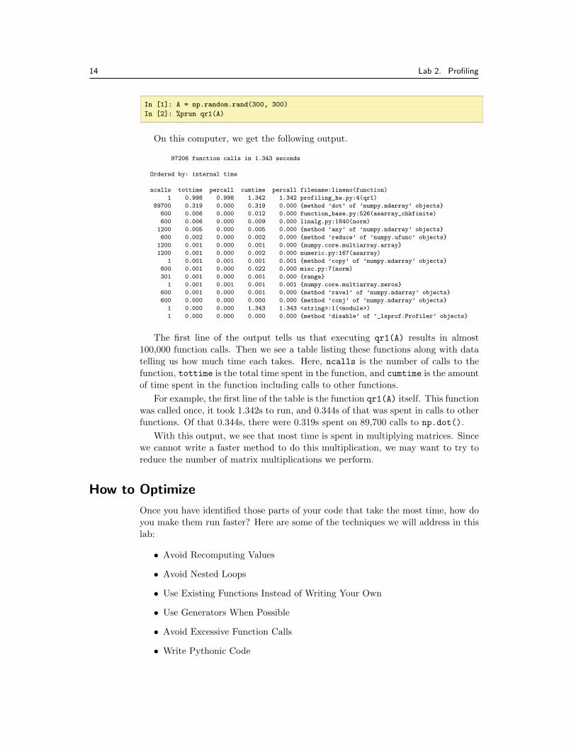
In [1]: A = np.random.rand(300, 300)
In [2]: %prun qr1(A)
On this computer, we get the following output.
97206 function calls in 1.343 seconds
Ordered by: internal time
ncalls tottime percall cumtime percall filename:lineno(function)
1 0.998 0.998 1.342 1.342 profiling_hw.py:4(qr1)
89700 0.319 0.000 0.319 0.000 {method ’dot’ of ’numpy.ndarray’ objects}
600 0.006 0.000 0.012 0.000 function_base.py:526(asarray_chkfinite)
600 0.006 0.000 0.009 0.000 linalg.py:1840(norm)
1200 0.005 0.000 0.005 0.000 {method ’any’ of ’numpy.ndarray’ objects}
600 0.002 0.000 0.002 0.000 {method ’reduce’ of ’numpy.ufunc’ objects}
1200 0.001 0.000 0.001 0.000 {numpy.core.multiarray.array}
1200 0.001 0.000 0.002 0.000 numeric.py:167(asarray)
1 0.001 0.001 0.001 0.001 {method ’copy’ of ’numpy.ndarray’ objects}
600 0.001 0.000 0.022 0.000 misc.py:7(norm)
301 0.001 0.000 0.001 0.000 {range}
1 0.001 0.001 0.001 0.001 {numpy.core.multiarray.zeros}
600 0.001 0.000 0.001 0.000 {method ’ravel’ of ’numpy.ndarray’ objects}
600 0.000 0.000 0.000 0.000 {method ’conj’ of ’numpy.ndarray’ objects}
1 0.000 0.000 1.343 1.343 <string>:1(<module>)
1 0.000 0.000 0.000 0.000 {method ’disable’ of ’_lsprof.Profiler’ objects}
The first line of the output tells us that executing qr1(A) results in almost
100,000 function calls. Then we see a table listing these functions along with data
telling us how much time each takes. Here, ncalls is the number of calls to the
function, tottime is the total time spent in the function, and cumtime is the amount
of time spent in the function including calls to other functions.
For example, the first line of the table is the function qr1(A) itself. This function
was called once, it took 1.342s to run, and 0.344s of that was spent in calls to other
functions. Of that 0.344s, there were 0.319s spent on 89,700 calls to np.dot().
With this output, we see that most time is spent in multiplying matrices. Since
we cannot write a faster method to do this multiplication, we may want to try to
reduce the number of matrix multiplications we perform.
How to Optimize
Once you have identified those parts of your code that take the most time, how do
you make them run faster? Here are some of the techniques we will address in this
lab:
• Avoid Recomputing Values
• Avoid Nested Loops
• Use Existing Functions Instead of Writing Your Own
• Use Generators When Possible
• Avoid Excessive Function Calls
• Write Pythonic Code

15
• Use Cython or Numba
• Use a More Efficient Algorithm
You should always use the profiling and timing functions to help you decide when
an optimization is actually useful.
Avoid Recomputing Values
In our function qr1(), we can avoid recomputing R[i,i] in the outer loop and
R[i,j] in the inner loop. The rewritten function is as follows:
def qr2(A):
ncols = A.shape[1]
Q = A.copy()
R = np.zeros((ncols, ncols))
for i in range(ncols):
R[i, i] = la.norm(Q[:, i])
Q[:, i] = Q[:, i]/R[i, i]
for j in range(i+1, ncols):
R[i, j] = Q[:, j].dot(Q[:, i])
Q[:,j] = Q[:,j]-R[i, j]*Q[:,i]
return Q, R
Profiling qr2() on a 300 × 300 matrix produces the following output.
48756 function calls in 1.047 seconds
Ordered by: internal time
ncalls tottime percall cumtime percall filename:lineno(function)
1 0.863 0.863 1.047 1.047 profiling_hw.py:16(qr2)
44850 0.171 0.000 0.171 0.000 {method ’dot’ of ’numpy.ndarray’ objects}
300 0.003 0.000 0.006 0.000 function_base.py:526(asarray_chkfinite)
300 0.003 0.000 0.005 0.000 linalg.py:1840(norm)
600 0.002 0.000 0.002 0.000 {method ’any’ of ’numpy.ndarray’ objects}
300 0.001 0.000 0.001 0.000 {method ’reduce’ of ’numpy.ufunc’ objects}
301 0.001 0.000 0.001 0.000 {range}
600 0.001 0.000 0.001 0.000 {numpy.core.multiarray.array}
600 0.001 0.000 0.001 0.000 numeric.py:167(asarray)
300 0.000 0.000 0.012 0.000 misc.py:7(norm)
1 0.000 0.000 0.000 0.000 {method ’copy’ of ’numpy.ndarray’ objects}
300 0.000 0.000 0.000 0.000 {method ’ravel’ of ’numpy.ndarray’ objects}
1 0.000 0.000 1.047 1.047 <string>:1(<module>)
300 0.000 0.000 0.000 0.000 {method ’conj’ of ’numpy.ndarray’ objects}
1 0.000 0.000 0.000 0.000 {numpy.core.multiarray.zeros}
1 0.000 0.000 0.000 0.000 {method ’disable’ of ’_lsprof.Profiler’ objects}
Our optimization reduced almost every kind of function call by half, and reduced
the total run time by 0.295s.
Some less obvious ways to eliminate excess computations include moving compu-
tations out of loops, not copying large data structures, and simplifying mathematical
expressions.
Avoid Nested Loops
For many algorithms, the temporal complexity of an algorithm is determined by the
loops. Nested loop quickly increase the temporal complexity. The best way to avoid

16 Lab 2. Profiling
nested loops is to use NumPy array operations instead of iterating through arrays.
If you must use nested loops, focus your optimization efforts on the innermost loop,
which gets called the most times.
Use Existing Functions Instead of Writing Your Own
If there is an intuitive operation you would like to perform on an array, chances
are that NumPy or another library already has a function that does it. Python
and NumPy functions have already been optimized, and are usually many times
faster than the equivalent you might write. We saw an example of this in Lab ??
where we compared NumPy array multiplication with our own matrix multiplication
implemented in Python.
Use Generators When Possible
When you are iterating through a list, you can often replace the list with a generator.
Instead of storing the entire list in memory, a generator computes each item as it
is needed. For example, the code
>>> for i in range(100):
... print i
stores the numbers 0 to 99 in memory, looks up each one in turn, and prints it. On
the other hand, the code
>>> for i in xrange(100):
... print i
uses a generator instead of a list. This code computes the first number in the
specified range (which is 0), and prints it. Then it computes the next number
(which is 1) and prints that.
It is also possible to write your own generators. See https://docs.python.org/
2/tutorial/classes.html#generators and https://wiki.python.org/moin/Generators
for more information.
In our example, replacing each range with xrange does not speed up qr2() by
a noticeable amount.
Avoid Excessive Function Calls
Function calls take time. Moreover, looking up methods associated with objects
takes time. Removing “dots” can significantly speed up execution time.
For example, we could rewrite our function to reduce the number of times we
need to look up the function la.norm().
def qr2(A):
norm = la.norm
ncols = A.shape[1]
Q = A.copy()
R = np.zeros((ncols, ncols))
for i in range(ncols):

17
R[i, i] = norm(Q[:, i])
Q[:, i] = Q[:, i]/R[i, i]
for j in range(i+1, ncols):
R[i, j] = Q[:, j].dot(Q[:, i])
Q[:,j] = Q[:,j]-R[i, j]*Q[:,i]
return Q, R
Once again, an analysis with %prun reveals that this optimization does not help
significantly in this case.
Write Pythonic Code
Several special features of Python allow you to write fast code easily. First, list
comprehensions are much faster than for loops. These are particularly useful when
building lists inside a loop. For example, replace
>>> mylist = []
>>> for i in xrange(100):
... mylist.append(math.sqrt(i))
with
>>> mylist = [math.sqrt(i) for i in xrange(100)]
When it can be used, the function map() is even faster.
>>> mylist = map(math.sqrt, xrange(100))
The analog of a list comprehension also exists for generators, dictionaries, and sets.
Second, swap values with a single assignment.
>>> a, b = 1, 2
>>> a, b = b, a
>>> print a, b
2 1
Third, many non-Boolean objects in Python have truth values. For example,
numbers are False when equal to zero and True otherwise. Similarly, lists and
strings are False when they are empty and True otherwise. So when a is a number,
instead of
>>> if a != 0:
use
>>> if a:
Problem 1. Using the profiling techniques discussed in this lab, find out
which portions of the code below require the most runtime. Then, rewrite
the function using some of the optimization techniques we have discussed
thus far.
18 Lab 2. Profiling
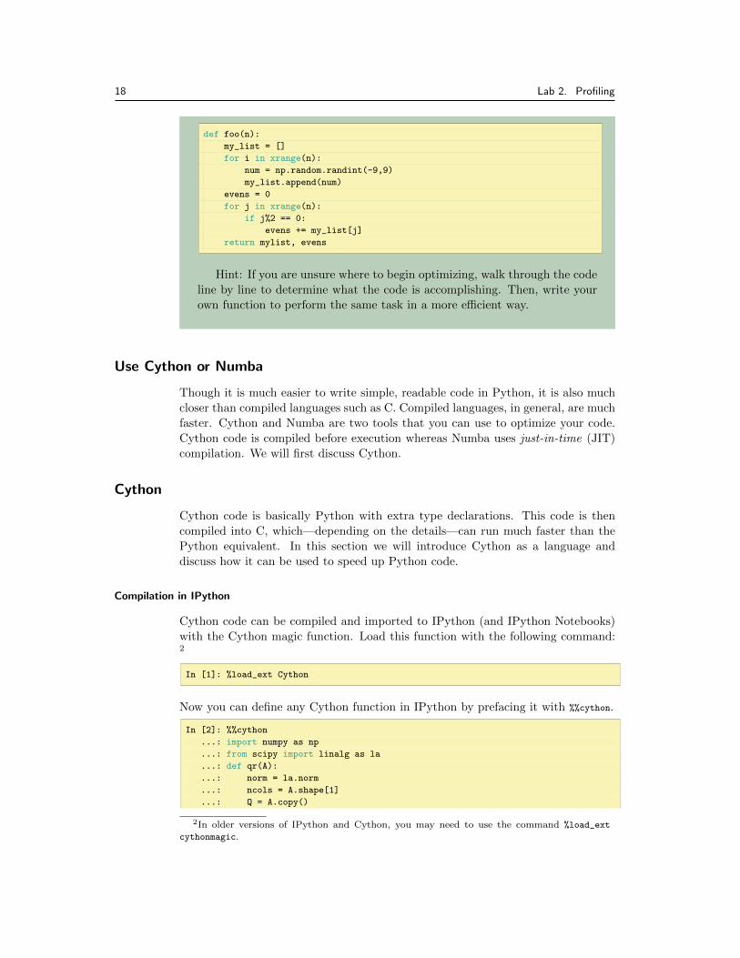
def foo(n):
my_list = []
for i in xrange(n):
num = np.random.randint(-9,9)
my_list.append(num)
evens = 0
for j in xrange(n):
if j%2 == 0:
evens += my_list[j]
return mylist, evens
Hint: If you are unsure where to begin optimizing, walk through the code
line by line to determine what the code is accomplishing. Then, write your
own function to perform the same task in a more efficient way.
Use Cython or Numba
Though it is much easier to write simple, readable code in Python, it is also much
closer than compiled languages such as C. Compiled languages, in general, are much
faster. Cython and Numba are two tools that you can use to optimize your code.
Cython code is compiled before execution whereas Numba uses just-in-time (JIT)
compilation. We will first discuss Cython.
Cython
Cython code is basically Python with extra type declarations. This code is then
compiled into C, which—depending on the details—can run much faster than the
Python equivalent. In this section we will introduce Cython as a language and
discuss how it can be used to speed up Python code.
Compilation in IPython
Cython code can be compiled and imported to IPython (and IPython Notebooks)
with the Cython magic function. Load this function with the following command:2
In [1]: %load_ext Cython
Now you can define any Cython function in IPython by prefacing it with %%cython.
In [2]: %%cython
...: import numpy as np
...: from scipy import linalg as la
...: def qr(A):
...: norm = la.norm
...: ncols = A.shape[1]
...: Q = A.copy()
2In older versions of IPython and Cython, you may need to use the command %load_ext
cythonmagic.

19
...: R = np.zeros((ncols, ncols))
...: for i in range(ncols):
...: R[i, i] = norm(Q[:, i])
...: Q[:, i] = Q[:, i]/R[i, i]
...: for j in range(i+1, ncols):
...: R[i, j] = Q[:, j].dot(Q[:, i])
...: Q[:,j] = Q[:,j]-R[i, j]*Q[:,i]
...: return Q, R
...:
Note the import statements on lines 2 and 3. Even if these modules were already
loaded in the current IPython session, these lines would still be necessary. Now the
qr() function has been compiled in Cython and can be called from IPython just as
any other function.
It is best to use this method of compilation if you are only using your optimized
funcion once or you are in the stages of developing your optimized algorithm. It can
be a little frustrating to fix errors in your function if you are using the IPython shell.
The IPython Notebook interface is much easier to use for these types of problems.
Compilation from the Command Line
Compiling Cython from the command line is particularly useful if you need an
optimized module that you will use over and over again. As we will discuss in this
section, once a function is written and compiled in Cython, it can be imported as
a module.
Cython code is usually written in a .pyx file, which is then compiled to C. Next
the C is compiled to a Python extension written in machine code. Figure ?? shows
how Cython code is compiled and called.
These two compilations (first to C and then to a Python extension) are accom-
plished by the script setup.py discussed earlier in this lab.
1 from distutils.core import setup
2 from Cython.Build import cythonize
4 setup(name="cymodule", ext_modules=cythonize('cymodule.pyx'))
setup.py
The call to cythonize() compiles cymodule.pyx to C, and the call to setup()
converts the C code to a Python extension.
Note
You can learn more about the Python/C balance in your Cython file with the
following line.
$ cython -a cymodule.pyx

20 Lab 2. Profiling
Compiled to runusing Python objects
Run withoutPython objects
Function callto compiled
C code
RunPythonCode
CythonCompiler
C Compiler
Python Code
Python VirtualMachine
Actual HardwareC Code Compiled
Into a Python-CompatibleExtension Module
Cython Code
C Code GeneratedFrom Cython Code
Figure 2.1: A diagram showing how Cython code is compiled and called. The path
from calling a Cython function in a Python file to its evaluation is shown in red.
This will generate a html file that you can open with your web browser. It will
show the lines that use Python in bright yellow and lines that use C in white.
Speeding up Cython with Type Declarations
So far, our Cythonized qr() function does not run any faster than the Python
version.3 The simplest way to take advantage of the C-compilation is to declare
data types, as you would in a C program. All Cython data types and their NumPy
equivalents are listed in Table ??.
Warning
Unlike Python integers, which can be arbitrarily large, Cython integers can
overflow.
In our example, when we declare the index j to be an int, the inner for loop
is pushed into C (instead of Python), speeding up our code immensely. We do this
by modifying cymodule.pyx as follows.
...
def qr():
cdef int j
ncols = A.shape[1]
Q = A.copy()
...
3Sometimes you will see speedup immediately after Cythonizing a Python function.

21
Cython Type NumPy Type Description
float float32 32 bit floating point number
double float64 64 bit floating point number
float complex complex64 64 bit floating point complex number
double complex complex128 128 bit floating point complex number
char int8 8 bit signed integer
unsigned char uint8 8 bit unsigned integer
short int16 16 bit signed integer
unsigned short uint16 16 bit unsigned integer
int int32 32 bit signed integer
unsigned int uint32 32 bit unsigned integer
long int32 or int64 32 or 64 bit signed integer (depends on
platform)
unsigned long uint32 or uint64 32 or 64 bit unsigned integer (depends
on platform )
long long int64 64 bit signed integer
unsigned long long uint64 64 bit unsigned integer
Table 2.1: Numeric types available in Cython.
We could also declare i to be an int, but the effect of doing so is negligible.After modifying cymodule.pyx, we must recompile it by running the script
setup.py, and then re-import it into Python. When we profile this function, wesee that it is indeed a good deal faster than its Python cousin, and all the speed upis in the function itself (where the for loops are).
...
ncalls tottime percall cumtime percall filename:lineno(function)
1 0.949 0.949 0.961 0.961 {cymodule.qr}
...
Similarly, you can speed up function calls in Cython by declaring the types of
some or all of the arguments.
def myfunction(double arg1, int arg2, arg3):
...
Arrays in Cython
You can also declare types for arrays. Doing so produces a typed memoryview, or
Cython array. As with ordinary variables, typed memoryviews can be initialized
when they are declared or later.
# Define a NumPy array
A = np.linspace(0,1,6)
# Create typed memoryviews on A and B
cdef double[:] cA = A
cdef int[:,:] cB
22 Lab 2. Profiling
# Initialize cB
cB = np.array([[1,2],[3,4],[5,6]], dtype=np.dtype("i"))
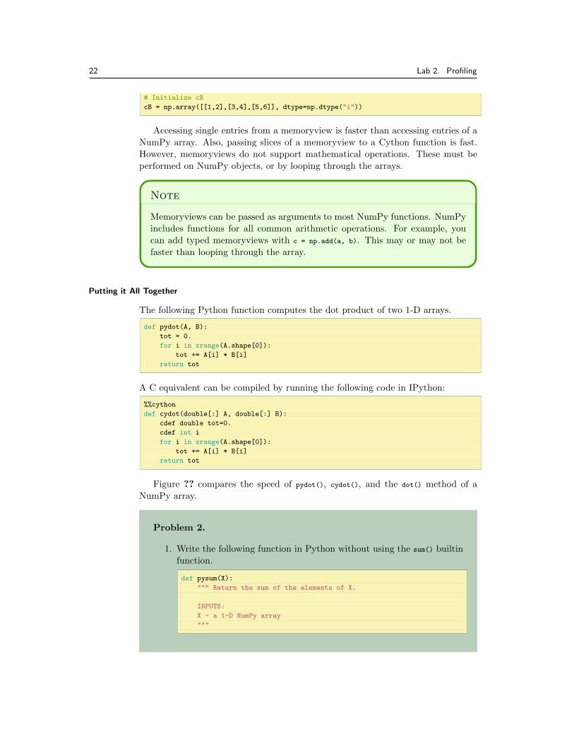
Accessing single entries from a memoryview is faster than accessing entries of a
NumPy array. Also, passing slices of a memoryview to a Cython function is fast.
However, memoryviews do not support mathematical operations. These must be
performed on NumPy objects, or by looping through the arrays.
Note
Memoryviews can be passed as arguments to most NumPy functions. NumPy
includes functions for all common arithmetic operations. For example, you
can add typed memoryviews with c = np.add(a, b). This may or may not be
faster than looping through the array.
Putting it All Together
The following Python function computes the dot product of two 1-D arrays.
def pydot(A, B):
tot = 0.
for i in xrange(A.shape[0]):
tot += A[i] * B[i]
return tot
A C equivalent can be compiled by running the following code in IPython:
%%cython
def cydot(double[:] A, double[:] B):
cdef double tot=0.
cdef int i
for i in xrange(A.shape[0]):
tot += A[i] * B[i]
return tot
Figure ?? compares the speed of pydot(), cydot(), and the dot() method of a
NumPy array.
Problem 2.
1. Write the following function in Python without using the sum() builtin
function.
def pysum(X):
""" Return the sum of the elements of X.
INPUTS:
X - a 1-D NumPy array
"""

23
Figure 2.2: The running times of pydot(), cydot(), and the dot() method of a NumPy
array on vectors of length “Array Size.” The Cython version runs almost as fast as
the version built into NumPy.
2. Rewrite the same function in Cython using a typed for-loop, and a
typed memoryview of X. Call this function cysum(). Assume the input
array X is an array of double precision floating point numbers.
3. Compare the pysum() function, the cysum(), the Python builtin sum()
function, and the np.sum() function. Print the results to the terminal.
Problem 3. In the Affine Transformations Lab (Lab ??) you wrote a func-
tion to compute the LU decomposition of a matrix. One possible implemen-
tation is found in the following code:
def LU(A):
"""Returns the LU decomposition of a square matrix."""
n = A.shape[0]
U = np.array(np.copy(A), dtype=float)
L = np.eye(n)
for i in xrange(1,n):
for j in xrange(i):

24 Lab 2. Profiling
L[i,j] = U[i,j]/U[j,j]
U[i,j:] -= L[i,j]*U[j,j:]
return L,U
1. Cython does not recognize NumPy array slicing. To be able to optimize
this function using Cython, all array slicing must be removed. Rewrite
the LU decomposition function so it performs every operation element-
by-element instead of using NumPy array operations.
2. Port your function from Part 1 to Cython. Use typed for-loops and
typed memoryviews. You may assume that you are only dealing with
real arrays of double precision floating point numbers.
3. Compare the speeds of the original code, your solution to Part 1, and
your solution to Part 2. Print the results to the terminal.
Numba
As mentioned before, Numba relies on a just-in-time (JIT) compiler. This means
that the code is compiled right before it is executed. We will discuss this process
a bit later in this section. The API for using Numba is incredibly simple. All one
has to do is import Numba and add the @jit function decorator to your function.
The following code would be a Numba equivalent to Problem ??.
from numba import jit
@jit
def numba_sum(A):
total = 0
for i in xrange(len(A)):
total += A[i]
return total
Though this code looks very simple, a lot is going on behind the scenes. As
we saw with Cython, our code will run faster if datatypes are assigned to all our
variables. With Cython, we had to explicitly definte the datatypes of each variable.
Rather than requiring us to define the datatypes explicitly, Numba attempts to
infer the correct datatypes based on the datatypes of the input.
In the code above, for example, say that our array A was full of integers. Though
we have not explicitly defined a datatype for the variable total, Numba will infer
that the datatype for total should also be an integer.
Once all the datatypes have been inferred and assigned, the code is translated
to machine code by the LLVM library. Numba will then cache this compiled version
of our code. This means that we can bypass this whole inference and compilation
process the next time we run our function.

25
More Control Within Numba
Though the inference engine within Numba does a good job, it’s not always perfect.
If you would like to have more control, you may specify datatypes explicity as
demonstrated in the code below.
Also, if you add the keyword argument, nopython=True to the jit decorator, an
error will be raised if Numba was unable to convert everything to explicit datatypes.
In this example, we will assume that the input will be doubles. Note that is
necessary to import the desired datatype from the Numba module.
from numba import double
@jit(nopython=True, locals=dict(A=double[:], total=double))
def numba_sum(A):
total = 0
for i in xrange(len(A)):
total += A[i]
return total
Notice that the jit function decorator is the only thing that changed. Note also that
this means that we will not be allowed to pass an array of integers to this function.
If we had not specified datatypes, the inference engine would allow us to pass arrays
of any numerical datatype. In the case that our function sees a datatype that it has
not seen before, the inference and compilation process would have to be repeated.
As before, the new version will also be cached.
If your function is running slower than you would expect, you can find out what
is going on under the hood by calling the inspect_types() method of the function.
# Due to the length of the output, we will leave it out of the lab text.
>>> numba_sum.inspect_types()
If you are trying to achieve the fastest runtimes possible, it will be worth trying
both Numba and Cython. Since Numba relies on an LLVM compiler and Cython
relies on a C compiler, it is possible that these two techniques will produce different
results.
Problem 4. The code below defines a Python function which takes a matrix
to the nth power.
def pymatpow(X, power):
""" Return X^{power}.
Inputs:
X (array) - A square 2-D NumPy array
power (int) - The power to which we are taking the matrix X.
Returns:
prod (array) - X^{power}
"""
prod = X.copy()
temparr = np.empty_like(X[0])
size = X.shape[0]
for n in xrange(1, power):
for i in xrange(size):

26 Lab 2. Profiling
for j in xrange(size):
tot = 0.
for k in xrange(size):
tot += prod[i,k] * X[k,j]
temparr[j] = tot
prod[i] = temparr
return prod
1. Port pymatpow() to Cython using typed for-loops and typed memo-
ryviews. Call your function cymatpow().
2. Create a compiled version of pymatpow() using Numba. Call this function
numbamatpow().
3. Compare the speed of pymatpow(), cymatpow(), numbamatpow() and the np.
dot() function. Remember to time numbamatpow() on the second pass so
the compilation process is not part of your timing. Print your results
to the terminal.
NumPy takes products of matrices by calling BLAS and LAPACK, which
are heavily optimized linear algebra libraries written in C, assembly, and
Fortran.
A Caution
NumPy’s array methods are often faster than a Cython or Numba equivalent you
could code yourself. If you are unsure which method is fastest, time them.
Moreover, a good algorithm written with a slow language (like Python) is faster
than a bad algorithm written in a fast language (like C). Hence, focus on writing
fast algorithms with good Python code, and only use Cython or Numba when and
where it is necessary.
Use a More Efficient Algorithm
The optimizations discussed thus far will speed up your code at most by a constant.
They will not change the complexity of your code. In order to reduce the complexity
(say from O(n2) to O(n log(n))), you typically need to change your algorithm. We
will address the benefits of using more efficient algorithms in Problem ??.
The correct choice of algorithm is more important than a fast implementation.
For example, suppose you wish to solve the following tridiagonal system.
b1 c1 0 0 · · · · · · 0
a1 b2 c2 0 · · · · · · 0
0 a2 b3 c3 · · · · · · 0...
......
.... . .
. . ....
......
......
. . .. . . cn−1
0 0 0 0 · · · an−1 bn
x1
x2
x3
...
...
xn
=
d1d2d3......
dn

27
One way to do this is with the general solve method in SciPy’s linalg module.
Alternatively, you could use an algorithm optimized for tridiagonal matrices. The
code below implements one such algorithm in Python. This is called the Thomas
algorithm.
The final result is stored in x, and c is used to store temporary values.
def pytridiag(a, b, c, x):
'''Solve the tridiagonal system Ad = x where A has diagonals a, b, and c.
INPUTS:
a, b, c, x - All 1-D NumPy arrays.
NOTE:
The final result is stored in `x` and `c` is used to store temporary values.
'''n = x.size
temp = 0.
c[0] /= b[0]
x[0] /= b[0]
for i in xrange(n-2):
temp = 1. / (b[i+1] - a[i] * c[i])
c[i+1] *= temp
x[i+1] = (x[i+1] - a[i] * x[i]) * temp
x[n-1] = (x[n-1] - a[n-2] * x[n-2]) / (b[n-1] - a[n-2] * c[n-2])
for i in xrange(n-2, -1, -1):
x[i] = x[i] - c[i] * x[i+1]
Problem 5.
1. Port the above code to Cython using typed for-loops, typed memo-
ryviews and appropriate compiler directives.
2. Compare the speed of your new function with pytridiag() and scipy.
linalg.solve(). To compare the first two functions, start with 1000000×1000000 sized systems. When testing the SciPy algorithm, start with
1000 × 1000 systems. You may use the code below to generate the
arrays, a, b, and c, along with the corresponding tridiagonal matrix A.
def init_tridiag(n):
"""Initializes a random nxn tridiagonal matrix A.
Inputs:
n (int) : size of array
Returns:
a (1-D array) : (-1)-th diagonal of A
b (1-D array) : main diagonal of A
c (1-D array) : (1)-th diagonal of A
A (2-D array) : nxn tridiagonal matrix defined by a,b,c.
"""
a = np.random.random_integers(-9,9,n).astype("float")
b = np.random.random_integers(-9,9,n).astype("float")
c = np.random.random_integers(-9,9,n).astype("float")

28 Lab 2. Profiling
A = np.zeros((b.size,b.size))
np.fill_diagonal(A,b)
np.fill_diagonal(A[1:,:-1],a)
np.fill_diagonal(A[:-1,1:],c)
return a,b,c,A
3. What do you learn about good implementation versus proper choice of
algorithm?
Note that an efficient tridiagonal matrix solver is implemented by scipy.
sparse.linalg.spsolve().
When to Stop Optimizing
You don’t need to apply every possible optimization to your code. When your code
runs acceptably fast, stop optimizing. There is no need spending valuable time
making optimizations once the speed is sufficient.
Moreover, remember not to prematurely optimize your functions. Make sure
the function does exactly what you want it to before worrying about any kind of
optimization.
More on Cython (Optional)
This section has a more complete introduction to Cython. For another reference,
see http://docs.cython.org/src/tutorial/cython_tutorial.html.
More on Type Declarations
Type declarations make Cython faster than Python because a computer can process
numbers faster when it knows ahead of time what type they are. Declaring a variable
type in Cython makes the variable a native machine type instead of a Python object.
You can initialize a variable when it is declared or afterwards. It is possible to
initialize several variables at once, as demonstrated below.
# Declare integer variables i, j, and k.
# Set k equal to 2.
cdef int i, j, k=2
cdef:
# Declare and initialize m equal to 4 and n equal to 5.
int m=4, n=5
# Declare and initialize e equal to 2.71.
double e = 2.71
# Declare a double precision complex number a.
double complex a

29
Compiler Directives
When you access elements of an array, Cython checks that the indices are within
bounds. Cython also allows negative indexing the same way Python does. These
features slow down code execution. After a program has been carefully debugged,
they may be removed via compiler directives.
Compiler directives in Cython can be included as comments or function deco-
rators. Directives included in comments will apply to the whole file, while function
decorators will only apply to the function immediately following. The comments to
turn off bounds checking and negative indices are
# cython: boundscheck=False
# cython: wraparound=False
To use the function decorators, first import the cython module by including the line
cimport cython in your import statements. The decorators are
cimport cython
@cython.boundscheck(False)
@cython.wraparound(False)
Cython has many other compiler directives, including cdivision. When cdivision
is set to True, the % operator returns a number with the sign of the first argument
(like in C). Also, division by 0 will no longer raise a ZeroDivisionError, which will
increase the speed of your program.
More on Functions in Cython
Speed up function calls in Cython by declaring the types of some or all of the
arguments.
def myfunction(double[:] X, int n, double h, items):
...
If we pass in a NumPy array for the argument X, Cython will convert it to a typed
memoryview before it enters the function. However, if we pass in a NumPy array
for items, it will remain a NumPy array in the function. Both typed and untyped
arguments can be made into keyword arguments.
Cython also allows you to make C functions that are only callable within the C
extension you are currently building. They are not ported into the Python names-
pace. These functions are declared using the same syntax as in Python, except the
keyword def is replaced with cdef. The keyword cpdef combines def and cdef by
creating two versions of the function: one for Python and one for C.
You can also specify the return type for functions declared using cdef and cpdef,
as in the code below.
cpdef int myfunction(double[:] X, int n, double h, items):
...
30 Lab 2. Profiling
More Examples
For another example, we will write functions which compute AAT from A. That is,
given A, these functions compute B where B[i,j] = dot(A[i],A[j]).
Here is the Python solution.
def pyrowdot(A):
B = np.empty((A.shape[0], A.shape[0]))
for i in xrange(A.shape[0]):
for j in xrange(i):
B[i,j] = pydot(A[i], A[j])
B[i,i] = pydot(A[i], A[i])
for i in xrange(A.shape[0]):
for j in xrange(i+1, A.shape[0]):
B[i,j] = B[j,i]
return B
Here is the Cython solution. We changed the function cydot() to a C function
since it will only be called by cyrowdot(). Also, the Cython solution uses a typed
memoryview of its input.
import numpy as np
cimport cython
# cython: boundscheck=False
# cython: wraparound=False
cpdef double cydot(double[:] A, double[:] B):
cdef double tot=0.
cdef int i, n=A.shape[0]
for i in xrange(n):
tot += A[i] * B[i]
return tot
def cyrowdot(double[:,:] A):
cdef double[:,:] B = np.empty((A.shape[0], A.shape[0]))
cdef int i, j, n=A.shape[0]
for i in xrange(n):
for j in xrange(i):
B[i,j] = cydot(A[i], A[j])
B[i,i] = cydot(A[i], A[i])
for i in xrange(n):
for j in xrange(i+1, n):
B[i,j] = B[j,i]
return np.array(B)
This can also be done in NumPy by running A.dot(A.T). The timings of pyrowdot
(), cyrowdot(), and the NumPy command A.dot(A.T) are shown in Figure ??.
In both of these examples, NumPy’s implementation was faster than the version
we wrote in Cython.

31
Figure 2.3: The timings of pyrowdot(), cyrowdot(), and the NumPy command A.dot(
A.T). The arrays used for testing were n× 3 where n is shown along the horizontal
axis.