l8 - db performance features - dit school of computing - db performance...create index emp_lastname...
TRANSCRIPT
16/10/16
1
Database Performance Features
Brendan Tierney
Database Performance Features/Issues
– Indexes – Parallel Queries – Par;;oning – Materialised Views
These are the main ones for DWs
There are lots of other DB Performance Features

16/10/16
2
How does the database retrieve the data • The important part of ROWID is the Data Block
• The data retrieves records in units of blocks • How does the data process the following query
SELECT * FROM Customers
• What about SELECT * FROM Customers WHERE County = ‘DUBLIN’
• Which is the most efficient / How many blocks does the queries return?
3
How does the database retrieve the data § Need to be able to locate the data
§ Need an address (loca;on on disk) § Reach record has a ROWID
SELECT ROWID, <column name list> FROM <table name> ROWID LAST_NAME -‐-‐-‐-‐-‐-‐-‐-‐-‐-‐-‐-‐-‐-‐-‐-‐-‐-‐ -‐-‐-‐-‐-‐-‐-‐-‐-‐-‐ AAAAaoAATAAABrXAAA BORTINS AAAAaoAATAAABrXAAE RUGGLES AAAAaoAATAAABrXAAG CHEN AAAAaoAATAAABrXAAN BLUMBERG
§ A ROWID has a four-‐piece format, OOOOOOFFFBBBBBBRRR: § OOOOOO: The data object number that iden;fies the database
segment (AAAAao in the example). Schema objects in the same segment, such as a cluster of tables, have the same data object number.
§ FFF: The tablespace-‐rela;ve datafile number of the datafile that contains the row (file AAT in the example).
§ BBBBBB: The data block that contains the row (block AAABrX in the example). Block numbers are rela;ve to their datafile, not tablespace. Therefore, two rows with iden;cal block numbers could reside in two different datafiles of the same tablespace.
§ RRR: The row in the block.
4

16/10/16
3
Suppor;ng Database Structures • Need to avoid full table scans
• Are there situa;ons when you need to do full scans
• Methods to improve performance • Clustering • Indexing
– B-‐tree – Func;on – Index Organised – Par;;oning – Bit Mapped
• Are there situa;ons when you need to do full scans • Situa;ons when using an index is not efficient • If so you will need to by-‐pass indexes
5
• What is an Index in a Database ?
• How does it work ?

16/10/16
4
Indexing § SELECT name § FROM student § WHERE student_id = ‘s123456789’
§ Need to look for an load every data block into memory § Then check to see if each record matches the WHERE clause
§ What if the table has 10, 100, 10000, 1000000 records
§ Need some way to easily identify the location of records for STUDENT_ID => ROWIDs needed § This mapping is called an Index
CREATE INDEX <Index Name> on <Table Name> (<Attribute List>)
§ Works in the same was as an index to a book
§ They also support referential integrity § When inserting a row into a table only need check the index on the table (PK Index) § To ensure FK to PK integrity § Much quicker than checking the table
7
Indexing – How are they created
8
§ Index consists of Afribute Value and ROWID
Sequential Indexing
16/10/16
5
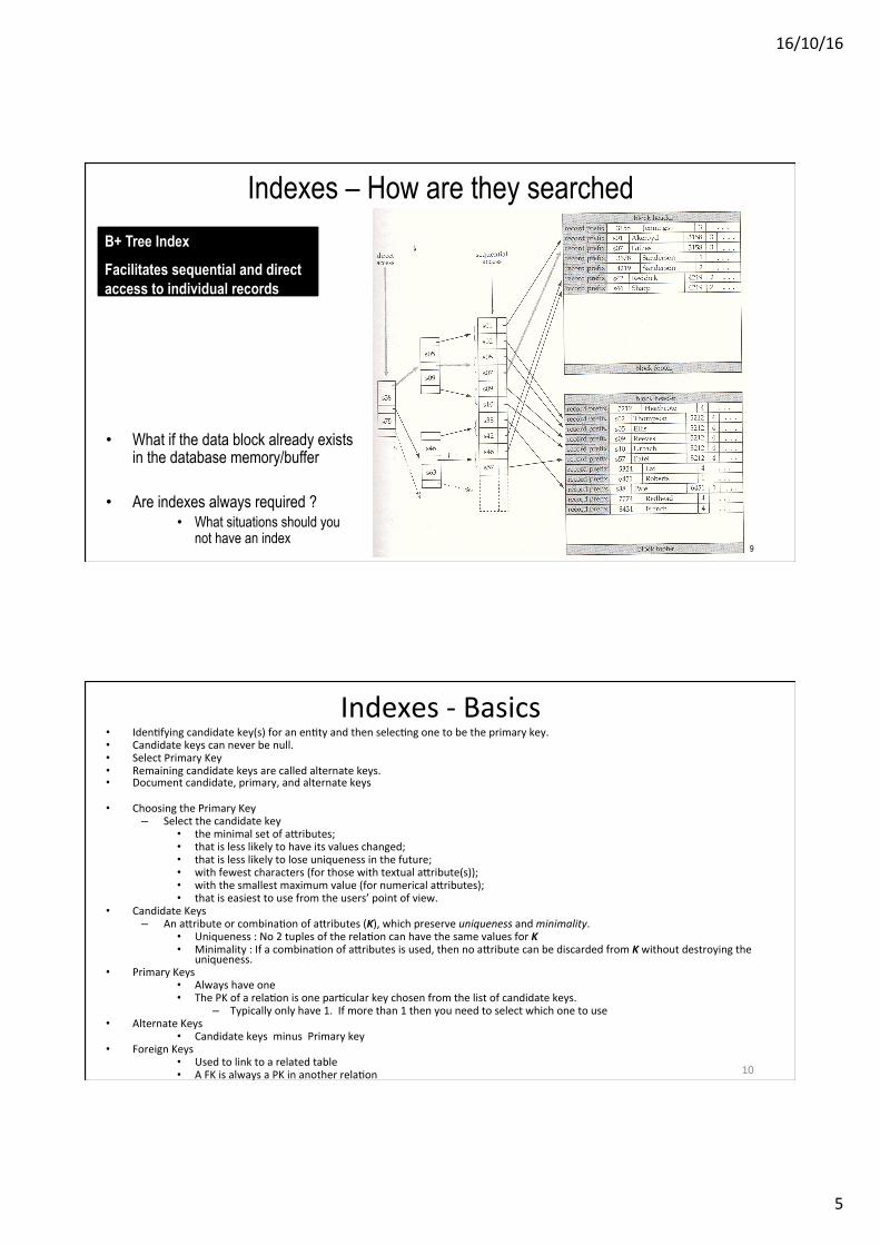
Indexes – How are they searched
9
• What if the data block already exists in the database memory/buffer
• Are indexes always required ? • What situations should you
not have an index
B+ Tree Index
Facilitates sequential and direct access to individual records
Indexes -‐ Basics • Iden;fying candidate key(s) for an en;ty and then selec;ng one to be the primary key. • Candidate keys can never be null. • Select Primary Key • Remaining candidate keys are called alternate keys. • Document candidate, primary, and alternate keys
• Choosing the Primary Key – Select the candidate key
• the minimal set of afributes; • that is less likely to have its values changed; • that is less likely to lose uniqueness in the future; • with fewest characters (for those with textual afribute(s)); • with the smallest maximum value (for numerical afributes); • that is easiest to use from the users’ point of view.
• Candidate Keys – An afribute or combina;on of afributes (K), which preserve uniqueness and minimality.
• Uniqueness : No 2 tuples of the rela;on can have the same values for K • Minimality : If a combina;on of afributes is used, then no afribute can be discarded from K without destroying the
uniqueness. • Primary Keys
• Always have one • The PK of a rela;on is one par;cular key chosen from the list of candidate keys.
– Typically only have 1. If more than 1 then you need to select which one to use • Alternate Keys
• Candidate keys minus Primary key • Foreign Keys
• Used to link to a related table • A FK is always a PK in another rela;on
10
16/10/16
6
Indexes -‐ Basics • Have to balance overhead in maintenance and use of secondary indexes against performance
improvement gained when retrieving data.
• This includes: – adding an index record to every secondary index whenever record is inserted; – upda;ng a secondary index when corresponding record is updated; – increase in disk space needed to store the secondary index; – possible performance degrada;on during query op;miza;on to consider all secondary indexes.
• General guidelines – (1) Do not index small tables. – (2) Index PK & FKs of a table – (3) Add secondary index to any column that is heavily used as a secondary key. – (4) Add secondary index on columns that are involved in: selec;on or join criteria; ORDER BY;
GROUP BY; and other opera;ons involving sor;ng (such as UNION or DISTINCT).
11
Indexes
• What should be indexed ? – If a column might be used as a predicate or join, then index it. – This probably means that nearly every column is going to be indexed. • You might be able to eliminate metric columns from considera;on if you are sure that no one is going to want to get a list of all retail transac;ons of greater than €1,000 for example.
• In a data warehouse, B-‐tree indexes should be used only for unique columns or other columns with very high cardinali;es
16/10/16
7
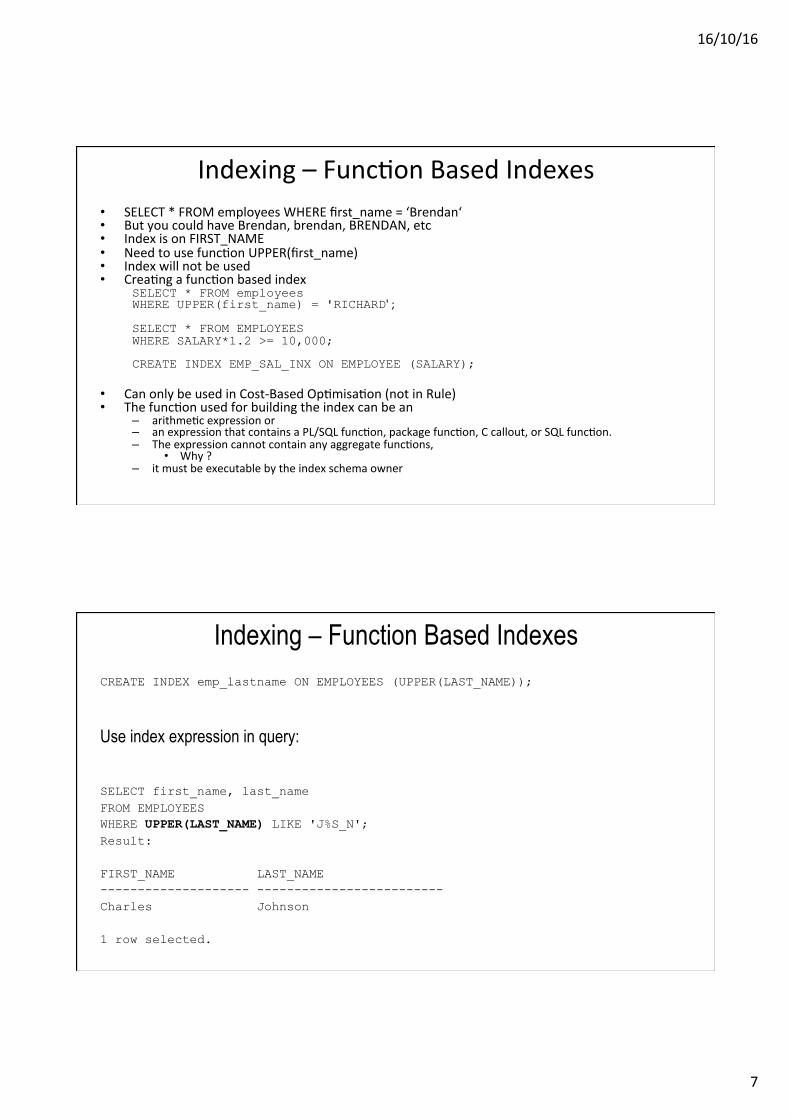
Indexing – Func;on Based Indexes • SELECT * FROM employees WHERE first_name = ‘Brendan‘ • But you could have Brendan, brendan, BRENDAN, etc • Index is on FIRST_NAME • Need to use func;on UPPER(first_name) • Index will not be used • Crea;ng a func;on based index
SELECT * FROM employees WHERE UPPER(first_name) = 'RICHARD' ; SELECT * FROM EMPLOYEES WHERE SALARY*1.2 >= 10,000; CREATE INDEX EMP_SAL_INX ON EMPLOYEE (SALARY);
• Can only be used in Cost-‐Based Op;misa;on (not in Rule) • The func;on used for building the index can be an
– arithme;c expression or – an expression that contains a PL/SQL func;on, package func;on, C callout, or SQL func;on. – The expression cannot contain any aggregate func;ons,
• Why ? – it must be executable by the index schema owner
Indexing – Function Based Indexes CREATE INDEX emp_lastname ON EMPLOYEES (UPPER(LAST_NAME));
Use index expression in query:
SELECT first_name, last_name FROM EMPLOYEES WHERE UPPER(LAST_NAME) LIKE 'J%S_N'; Result: FIRST_NAME LAST_NAME -------------------- ------------------------- Charles Johnson 1 row selected.
16/10/16
8
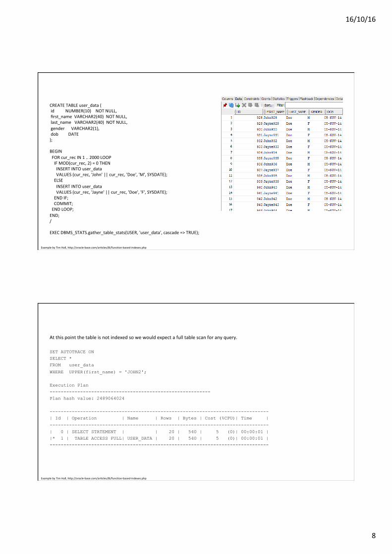
CREATE TABLE user_data ( id NUMBER(10) NOT NULL, first_name VARCHAR2(40) NOT NULL, last_name VARCHAR2(40) NOT NULL, gender VARCHAR2(1), dob DATE ); BEGIN FOR cur_rec IN 1 .. 2000 LOOP IF MOD(cur_rec, 2) = 0 THEN INSERT INTO user_data VALUES (cur_rec, 'John' || cur_rec, 'Doe', 'M', SYSDATE); ELSE INSERT INTO user_data VALUES (cur_rec, 'Jayne' || cur_rec, 'Doe', 'F', SYSDATE); END IF; COMMIT; END LOOP; END; / EXEC DBMS_STATS.gather_table_stats(USER, 'user_data', cascade => TRUE);
Example by Tim Hall, hfp://oracle-‐base.com/ar;cles/8i/func;on-‐based-‐indexes.php
At this point the table is not indexed so we would expect a full table scan for any query. SET AUTOTRACE ON
SELECT *
FROM user_data
WHERE UPPER(first_name) = 'JOHN2';
Execution Plan
----------------------------------------------------------
Plan hash value: 2489064024
-------------------------------------------------------------------------------
| Id | Operation | Name | Rows | Bytes | Cost (%CPU)| Time |
-------------------------------------------------------------------------------
| 0 | SELECT STATEMENT | | 20 | 540 | 5 (0)| 00:00:01 |
|* 1 | TABLE ACCESS FULL| USER_DATA | 20 | 540 | 5 (0)| 00:00:01 |
-------------------------------------------------------------------------------
Example by Tim Hall, hfp://oracle-‐base.com/ar;cles/8i/func;on-‐based-‐indexes.php

16/10/16
9
Build Regular Index
If we now create a regular index on the FIRST_NAME column we see that the index is not used. CREATE INDEX first_name_idx ON user_data (first_name); EXEC DBMS_STATS.gather_table_stats(USER, 'user_data', cascade => TRUE); SET AUTOTRACE ON SELECT * FROM user_data WHERE UPPER(first_name) = 'JOHN2'; Execution Plan ---------------------------------------------------------- Plan hash value: 2489064024 ------------------------------------------------------------------------------- | Id | Operation | Name | Rows | Bytes | Cost (%CPU)| Time | ------------------------------------------------------------------------------- | 0 | SELECT STATEMENT | | 20 | 540 | 5 (0)| 00:00:01 | |* 1 | TABLE ACCESS FULL| USER_DATA | 20 | 540 | 5 (0)| 00:00:01 | -------------------------------------------------------------------------------
Example by Tim Hall, hfp://oracle-‐base.com/ar;cles/8i/func;on-‐based-‐indexes.php
Build Func:on Based Index If we now replace the regular index with a func;on based index on the FIRST_NAME column we see that the index is used. DROP INDEX first_name_idx; CREATE INDEX first_name_idx ON user_data (UPPER(first_name)); EXEC DBMS_STATS.gather_table_stats(USER, 'user_data', cascade => TRUE); SET AUTOTRACE ON SELECT * FROM user_data WHERE UPPER(first_name) = 'JOHN2'; Execution Plan ---------------------------------------------------------- Plan hash value: 1309354431 ---------------------------------------------------------------------------------------------- | Id | Operation | Name | Rows | Bytes | Cost (%CPU)| Time | ---------------------------------------------------------------------------------------------- | 0 | SELECT STATEMENT | | 1 | 36 | 2 (0)| 00:00:01 | | 1 | TABLE ACCESS BY INDEX ROWID| USER_DATA | 1 | 36 | 2 (0)| 00:00:01 | |* 2 | INDEX RANGE SCAN | FIRST_NAME_IDX | 1 | | 1 (0)| 00:00:01 | ----------------------------------------------------------------------------------------------
Example by Tim Hall, hfp://oracle-‐base.com/ar;cles/8i/func;on-‐based-‐indexes.php

16/10/16
10
Concatenated Columns This method works for concatenated indexes also. DROP INDEX first_name_idx; CREATE INDEX first_name_idx ON user_data (gender, UPPER(first_name), dob); EXEC DBMS_STATS.gather_table_stats(USER, 'user_data', cascade => TRUE); SET AUTOTRACE ON SELECT * FROM user_data WHERE gender = 'M' AND UPPER(first_name) = 'JOHN2'; Execution Plan ---------------------------------------------------------- Plan hash value: 1309354431 ---------------------------------------------------------------------------------------------- | Id | Operation | Name | Rows | Bytes | Cost (%CPU)| Time | ---------------------------------------------------------------------------------------------- | 0 | SELECT STATEMENT | | 1 | 36 | 3 (0)| 00:00:01 | | 1 | TABLE ACCESS BY INDEX ROWID| USER_DATA | 1 | 36 | 3 (0)| 00:00:01 | |* 2 | INDEX RANGE SCAN | FIRST_NAME_IDX | 1 | | 2 (0)| 00:00:01 | ----------------------------------------------------------------------------------------------
Example by Tim Hall, hfp://oracle-‐base.com/ar;cles/8i/func;on-‐based-‐indexes.php
Indexing – Index Organised Tables • Storage organiza;on is a variant of a primary B-‐tree.
– Unlike an ordinary table whose data is stored as an unordered collec;on, data for an index-‐organized table is stored in a B-‐tree index structure in a primary key sorted manner. – Besides storing the primary key column values of an index-‐organized table row, each index entry in the B-‐tree stores the non-‐key column values as well.
– An index-‐organized table configura;on is similar to an ordinary table and an index on one or more of the table columns – but instead of maintaining two separate storage structures
• one for the table and one for the B-‐tree index – The database system maintains only a single B-‐tree index. – The ROWID is not stored in the index entry, the non-‐key column values are stored. – An Index Organised Table consists of an index that contains
• <primary_key_value, non_primary_key_column_values>.

16/10/16
11
Indexing – Index Organised Tables
Ordinary Table Index-‐Organised Table
ROWID uniquely iden;fies a row. Primary Key uniquely iden;fies rows
Access based on ROWID Access based on logical ROWID
Sequen;al scan returns all rows Full index scan returns all rows
21
Indexes – Bitmap Indexes
• Bitmap Indexes – The advantages of using bitmap indexes are greatest for columns in which the
ra;o of the number of dis;nct values to the number of rows in the table is small.
– This ra;o as the degree of cardinality – For example, on a table with one million rows, a column with 10,000 dis;nct
values is a candidate for a bitmap index. – A bitmap index on this column can outperform a B-‐tree index, par;cularly
when this column is oyen queried in conjunc;on with other indexed columns. – A bitmap index can be considered for any non-‐unique column.
• B-‐tree indexes are most effec;ve for high-‐cardinality data: that is, for data with many possible values, such as customer_name or phone_number
• Primary Keys
16/10/16
12
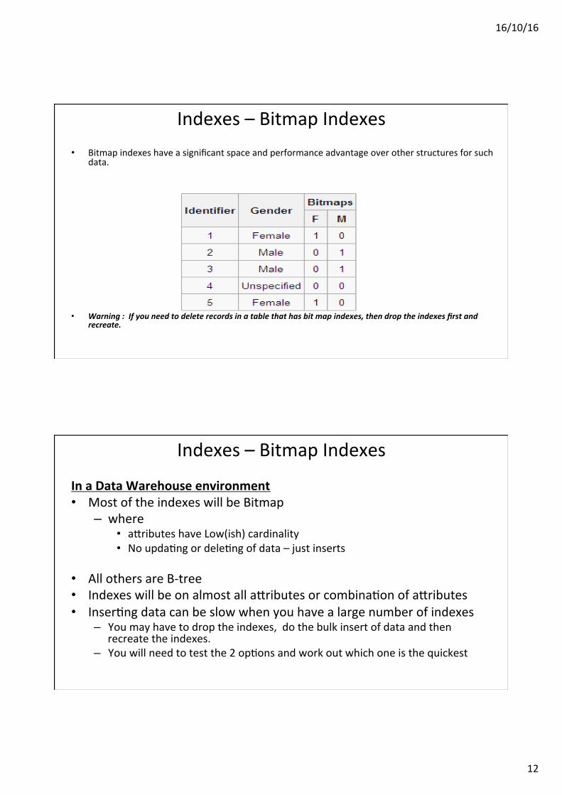
Indexes – Bitmap Indexes • Bitmap indexes have a significant space and performance advantage over other structures for such
data. • Bitmap indexes use bit arrays and answer queries by performing bitwise logical opera;ons on
these bitmaps.
• Warning : If you need to delete records in a table that has bit map indexes, then drop the indexes first and recreate.
Indexes – Bitmap Indexes
In a Data Warehouse environment • Most of the indexes will be Bitmap
– where • afributes have Low(ish) cardinality • No upda;ng or dele;ng of data – just inserts
• All others are B-‐tree • Indexes will be on almost all afributes or combina;on of afributes • Inser;ng data can be slow when you have a large number of indexes
– You may have to drop the indexes, do the bulk insert of data and then recreate the indexes.
– You will need to test the 2 op;ons and work out which one is the quickest
16/10/16
13
Indexes – What Columns should you index? § “I don’t know what the users will query on so let’s index everything”
§ But you do know how they will search!! How?
§ Scenarios when you don’t know?
§ Indexing is part of the (physical) Database Design process § Will also be part of the Testing phase § Every day task for the DBA/DB Designer.
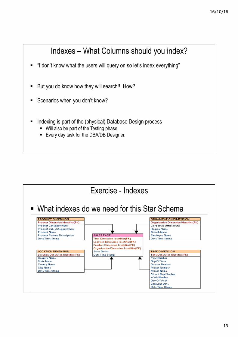
Exercise - Indexes
§ What indexes do we need for this Star Schema

16/10/16
14
Parallel Queries
• Parallel execu;on drama;cally reduces response ;me for data-‐intensive opera;ons on large databases
• Parallelism is the idea of breaking down a task so that, instead of one process doing all of the work in a query, many processes do part of the work at the same ;me. – The statement being processed can be split up among many CPUs on a single
Oracle system – An example of this is when four processes handle four different quarters in a year
instead of one process handling all four quarters by itself.
Parallel Queries
§ For a normal query in a database the server process performs all necessary processing for the sequen;al execu;on of a SQL statement. § For example, to perform a full table scan (such as SELECT * FROM emp), one
process performs the en;re opera;on

16/10/16
15
Parallel Queries • If we perform the same query using Parallel execu;on, the database server breaks the query
into a number of processes and executes these processed to get the data. • The table is divided dynamically based on the number of blocks for the table
• The Degree of Parallelism (DOP) is the number of parallel execu;on servers assigned to a single opera;on
Parallel Queries – Select statement
• Specified as a query hint
SELECT /*+ PARALLEL(orders, 4) */ COUNT(*) FROM orders;
SELECT /*+ PARALLEL(employees 4) PARALLEL(departments 2) */ MAX(salary), AVG(salary) FROM employees, departments WHERE employees.department_id = departments.department_id GROUP BY employees.department_id;
16/10/16
16
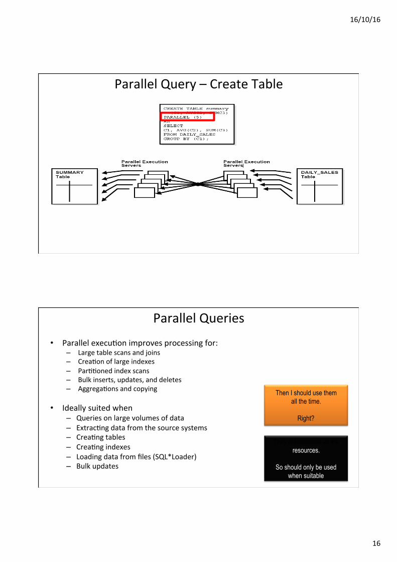
Parallel Query – Create Table
INSERT /*+ PARALLEL(tbl_ins,2) */ INTO tbl_ins SELECT /*+ PARALLEL(tbl_sel,4) */ * FROM tbl_sel;
Parallel Queries
• Parallel execu;on improves processing for: – Large table scans and joins – Crea;on of large indexes – Par;;oned index scans – Bulk inserts, updates, and deletes – Aggrega;ons and copying
• Ideally suited when – Queries on large volumes of data – Extrac;ng data from the source systems – Crea;ng tables – Crea;ng indexes – Loading data from files (SQL*Loader) – Bulk updates
Then I should use them all the time.
Right?
They will consume all the resources.
So should only be used
when suitable

16/10/16
17
Parallel Queries • Degree of Parallelism (DOP)
• Lowest value is 2 • Max is determined by the number of CPUS etc available • You will need to test to find the appropriate value for DOP
– It also depends on what else is running on the server at the same ;me – Par;cularly during the extrac;on process from the source systems
• Exercise to test Parallel Query • Create a table with 500,000 records • Create a table with 1M records, 2M records, … up to 10M records • Issues a Select statement without using parallelism on each table
– SQL> set ;me on -‐ to get the start and end ;mes • Then issue the same query with
– Parallel (<table name>, 2) – Parallel (<table name>, 4) – Parallel (<table name>, 6) – Parallel (<table name>, 8)
Data / Table Partitioning
34
• Partitioning is useful for many different types of applications, particularly applications that manage large volumes of data. OLTP systems often benefit from improvements in manageability and availability, while data warehousing systems benefit from performance and manageability
16/10/16
18
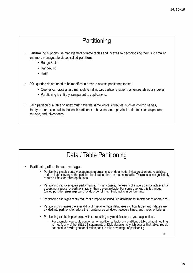
Partitioning • Partitioning supports the management of large tables and indexes by decomposing them into smaller
and more manageable pieces called partitions. • Range & List • Range-List • Hash
• SQL queries do not need to be modified in order to access partitioned tables. • Queries can access and manipulate individuals partitions rather than entire tables or indexes. • Partitioning is entirely transparent to applications.
• Each partition of a table or index must have the same logical attributes, such as column names, datatypes, and constraints, but each partition can have separate physical attributes such as pctfree, pctused, and tablespaces.
Data / Table Partitioning • Partitioning offers these advantages:
• Partitioning enables data management operations such data loads, index creation and rebuilding, and backup/recovery at the partition level, rather than on the entire table. This results in significantly reduced times for these operations.
• Partitioning improves query performance. In many cases, the results of a query can be achieved by accessing a subset of partitions, rather than the entire table. For some queries, this technique (called partition pruning) can provide order-of-magnitude gains in performance.
• Partitioning can significantly reduce the impact of scheduled downtime for maintenance operations.
• Partitioning increases the availability of mission-critical databases if critical tables and indexes are divided into partitions to reduce the maintenance windows, recovery times, and impact of failures.
• Partitioning can be implemented without requiring any modifications to your applications. – For example, you could convert a non-partitioned table to a partitioned table without needing
to modify any of the SELECT statements or DML statements which access that table. You do not need to rewrite your application code to take advantage of partitioning.
36

16/10/16
19
Data / Table Partitioning • Range Partitioning
• Range partitioning maps data to partitions based on ranges of partition key values that you establish for each partition.
• It is the most common type of partitioning and is often used with dates. – For example, you might want to partition sales data into monthly partitions
CREATE TABLE sales_range ( salesman_id NUMBER(5), salesman_name VARCHAR2(30), sales_amount NUMBER(10), sales_date DATE) PARTITION BY RANGE(sales_date) ( PARTITION sales_jan2000 VALUES LESS THAN(TO_DATE('02/01/2000','DD/MM/YYYY')), PARTITION sales_feb2000 VALUES LESS THAN(TO_DATE('03/01/2000','DD/MM/YYYY')), PARTITION sales_mar2000 VALUES LESS THAN(TO_DATE('04/01/2000','DD/MM/YYYY')), PARTITION sales_apr2000 VALUES LESS THAN(TO_DATE('05/01/2000','DD/MM/
YYYY')) );
37
Data / Table Partitioning § List Partitioning
• Enables you to explicitly control how rows map to partitions. • Done by specifying a list of discrete values for the partitioning key in the description for each partition. • This is different from range partitioning, where a range of values is associated with a partition. • The advantage of list partitioning is that you can group and organize unordered and unrelated sets of
data in a natural way. CREATE TABLE sales_list ( salesman_id NUMBER(5), salesman_name VARCHAR2(30), sales_state VARCHAR2(20), sales_amount NUMBER(10), sales_date DATE) PARTITION BY LIST(sales_state) ( PARTITION sales_west VALUES('California', 'Hawaii'), PARTITION sales_east VALUES ('New York', 'Virginia', 'Florida'), PARTITION sales_central VALUES('Texas', 'Illinois') PARTITION sales_other VALUES(DEFAULT) );
38
16/10/16
20
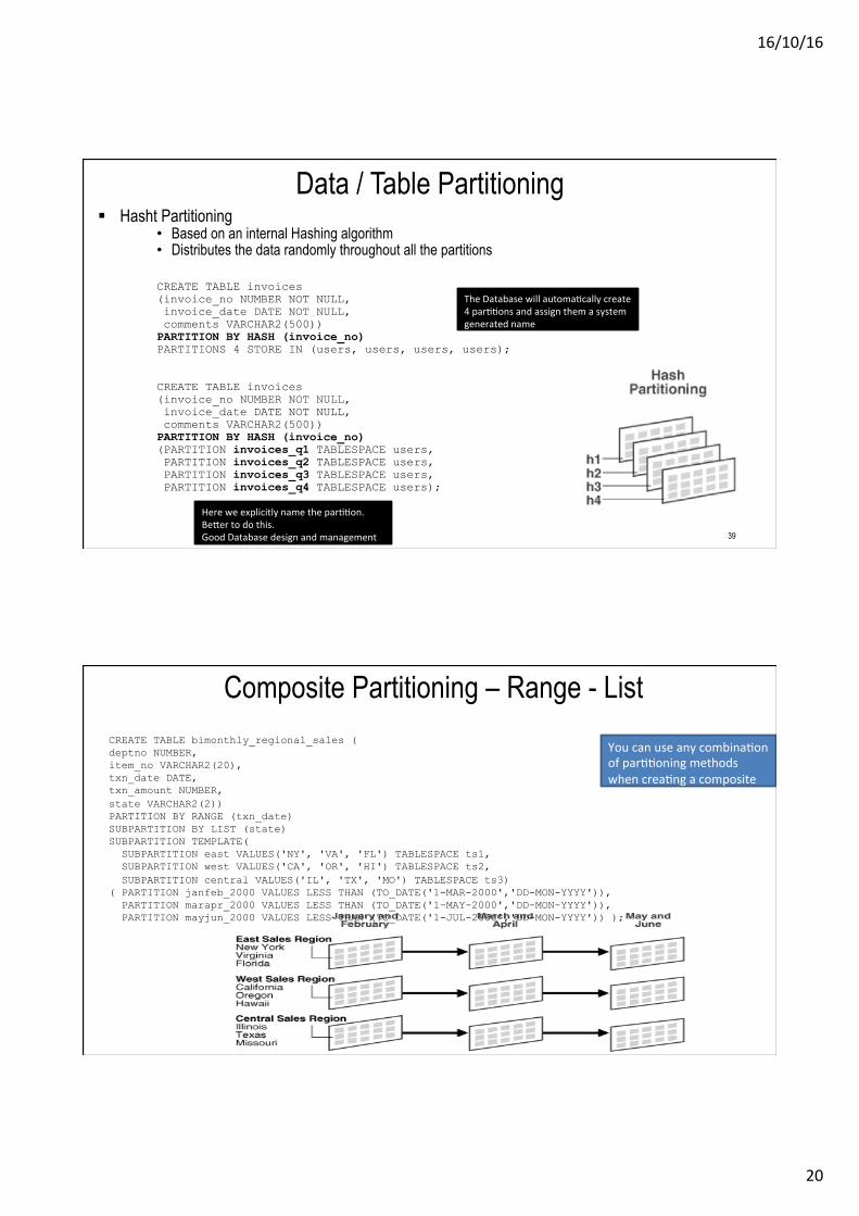
Data / Table Partitioning § Hasht Partitioning
• Based on an internal Hashing algorithm • Distributes the data randomly throughout all the partitions CREATE TABLE invoices (invoice_no NUMBER NOT NULL, invoice_date DATE NOT NULL, comments VARCHAR2(500)) PARTITION BY HASH (invoice_no) PARTITIONS 4 STORE IN (users, users, users, users); CREATE TABLE invoices (invoice_no NUMBER NOT NULL, invoice_date DATE NOT NULL, comments VARCHAR2(500)) PARTITION BY HASH (invoice_no) (PARTITION invoices_q1 TABLESPACE users, PARTITION invoices_q2 TABLESPACE users, PARTITION invoices_q3 TABLESPACE users, PARTITION invoices_q4 TABLESPACE users);
39
The Database will automa;cally create 4 par;;ons and assign them a system generated name
Here we explicitly name the par;;on. Befer to do this. Good Database design and management
Composite Partitioning – Range - List CREATE TABLE bimonthly_regional_sales ( deptno NUMBER, item_no VARCHAR2(20), txn_date DATE, txn_amount NUMBER, state VARCHAR2(2)) PARTITION BY RANGE (txn_date) SUBPARTITION BY LIST (state) SUBPARTITION TEMPLATE( SUBPARTITION east VALUES('NY', 'VA', 'FL') TABLESPACE ts1, SUBPARTITION west VALUES('CA', 'OR', 'HI') TABLESPACE ts2, SUBPARTITION central VALUES('IL', 'TX', 'MO') TABLESPACE ts3) ( PARTITION janfeb_2000 VALUES LESS THAN (TO_DATE('1-MAR-2000','DD-MON-YYYY')), PARTITION marapr_2000 VALUES LESS THAN (TO_DATE('1-MAY-2000','DD-MON-YYYY')), PARTITION mayjun_2000 VALUES LESS THAN (TO_DATE('1-JUL-2000','DD-MON-YYYY')) );
You can use any combina;on of par;;oning methods when crea;ng a composite

16/10/16
21
Partitioning - Indexes
• Indexes can be created using partitioning
CREATE INDEX cost_ix ON sales (amount_sold) GLOBAL PARTITION BY RANGE (amount_sold)
( PARTITION p1 VALUES LESS THAN (1000), PARTITION p2 VALUES LESS THAN (2500), PARTITION p3 VALUES LESS THAN (MAXVALUE));
The same par;;oning methods can be applied when crea;ng indexes
Maybe use the same par;;oning method on table and index. But you don’t have too.
Partitioning
• Very suited to a data warehouse environment as it can greatly increase performance.
• Suited to tables (and indexes) where >2M records and there is a natural (even-ish) distribution of data
• Typically you would partition the Fact table in a DW • Based on the Time Dimension as most of the queries will be
accessing the data based on dates
Non partitioned table Partitioned table
Stored in one tablespace Each Partition can be stored in separate tablespaces

16/10/16
22
Materialised Views
• Materialized views are query results that have been stored in advance so long-running calculations are not necessary when queries are executed.
• It is not untypical for DW queries to take >5, 10, 30, 60 minutes • For standardised queries that are run frequently during the day, MVs can give significant
performance improvement • MVs are typically used summary tables/views
• In a real-time environment they can be used to give current information • You can set a Refresh frequency
Results Regular views are computed each ;me the view is accessed
With MVs the data is cached a predefined ;mes The query is run once. All users select from the cached results
Materialised Views
CREATE MATERIALIZED VIEW all_customers PCTFREE 5 PCTUSED 60 TABLESPACE example
STORAGE (INITIAL 50K NEXT 50K) USING INDEX STORAGE (INITIAL 25K NEXT 25K) REFRESH START WITH ROUND(SYSDATE + 1) + 11/24
NEXT NEXT_DAY(TRUNC(SYSDATE), 'MONDAY') + 15/24 AS SELECT * FROM sh.customers@remote UNION SELECT * FROM sh.customers@local;
• Automatically refreshes this materialized view tomorrow at 11:00 a.m. and subsequently every Monday at 3:00 p.m

16/10/16
23
Clustering
45
Clustering • A cluster is a group of tables that share the same data blocks
– They share common columns and are often used together. – Example
• Employees and Departments table share the department_id column. • When you cluster the employees and departments tables the DB physically stores all rows for each
department from both the employees and departments tables in the same data blocks. – clusters offers these benefits: – Disk I/O is reduced for joins of clustered tables. – Access time improves for joins of clustered tables. – In a cluster, a cluster key value is the value of the cluster key columns for a particular row.
• Each cluster key value is stored only once each in the cluster and the cluster index, no matter how many rows of different tables contain the value.
• Therefore, less storage is required to store related table and index data in a cluster than is necessary in non-clustered table format.
• Example shows how each cluster key (each department_id) is stored just once for many rows that contain the same value in both the employees and departments tables
46

16/10/16
24
Clustering • Records can be randomly distributed • If they were grouped logically together then
• Easier to locate the required data & number of disk accesses would be lower • Records to be stored (clustered) together in the same or adjacent block • This approach is most suitable to bulk/batch processing on specific segments of the data • Example
– Suppose we have a Student table for all students in Ireland – Types of queries/processing might be on location, year of study
» Location = Dublin 8 » All students who live in Dublin 8 will have their records physically stored beside each other
• Can have a large database management overhead • May involve database reorganisation when new data is inserted • Because new records needs to be located beside existing data • This may require data or blocks being moved to another location
• Requires insight into expected use and frequency of different types of request • This applies to all approaches • Need to work out appropriate methods to implement
– Requires skill and experience • Need to monitor continually and make changes if necessary
47
Many things to consider when writing your SQL § We have looked at a number ways and things to consider when writing your SQL
§ But is there anything else that I need to consider ?
§ What about how the results are presented ?
§ Remember all the data/results are sent over the network
§ Can the database and network work together so that I can get my data quicker

16/10/16
25
Networking Compression of Query Results § Oracle Example – Sorry !!! § When you array fetch data from the database, SQL*Net will write the first row in
its entirety on the network. § When it goes to write the second row however, it will only transmit column values
that differ from the first row. § The third row written on the network will similarly be only the changed values
from the second row, and so on. § This compression therefore works well with repetitive data - of which we have a
lot typically! § This compression works even better with data that is sorted by these repeating
values so that the repeating values are near each other in the result set.
The key to this is
§ How can we ensure this repetition will happen?
§ We need a ORDER BY on our SELECT statements
§ The compression works even better with data that is sorted by these repeating values so that the repeating values are near each other in the result set.

16/10/16
26
Example to illustrate § We need to set up some data
§ This newly created table is about 8MB in size and consists of 1,031 blocks in my database – number will differ from Env to Env
§ Additionally, this table stores about 70 rows per block – there are about 72,000 rows on 1,031 blocks.
Setting up the baseline test § Select the entire contents of the table over the network using SQL*Plus
§ 8Mb of data was transferred from the DB server to the client machine
§ The array size is enough for 15 records. § So this equate to approx. 5 reads to get one block of data
16/10/16
27
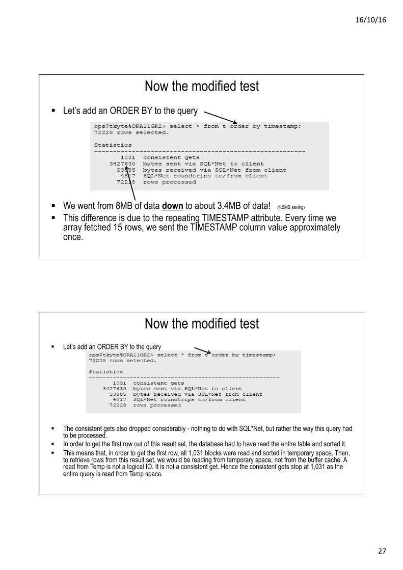
Now the modified test § Let’s add an ORDER BY to the query
§ We went from 8MB of data down to about 3.4MB of data! (4.5MB saving) § This difference is due to the repeating TIMESTAMP attribute. Every time we
array fetched 15 rows, we sent the TIMESTAMP column value approximately once.
Now the modified test § Let’s add an ORDER BY to the query
§ The consistent gets also dropped considerably - nothing to do with SQL*Net, but rather the way this query had to be processed.
§ In order to get the first row out of this result set, the database had to have read the entire table and sorted it. § This means that, in order to get the first row, all 1,031 blocks were read and sorted in temporary space. Then,
to retrieve rows from this result set, we would be reading from temporary space, not from the buffer cache. A read from Temp is not a logical IO. It is not a consistent get. Hence the consistent gets stop at 1,031 as the entire query is read from Temp space.