l3: review of linear algebra and matlabcourses.cs.tamu.edu/rgutier/csce666_f16/l3.pdf · l3: review...

CSCE 666 Pattern Analysis | Ricardo Gutierrez-Osuna | CSE@TAMU 1

L3: Review of linear algebra and MATLAB

• Vector and matrix notation

• Vectors

• Matrices

• Vector spaces

• Linear transformations

• Eigenvalues and eigenvectors

• MATLAB® primer


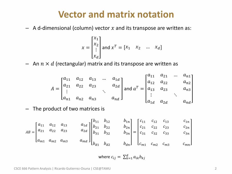
Vector and matrix notation – A d-dimensional (column) vector 𝑥 and its transpose are written as:

𝑥 =

𝑥1𝑥2⋮𝑥𝑑

and 𝑥𝑇 = 𝑥1 𝑥2 … 𝑥𝑑

– An 𝑛 × 𝑑 (rectangular) matrix and its transpose are written as

𝐴 =

𝑎11 𝑎12 𝑎13 … 𝑎1𝑑𝑎21 𝑎22 𝑎23 𝑎2𝑑⋮ ⋱𝑎𝑛1 𝑎𝑛2 𝑎𝑛3 𝑎𝑛𝑑

and 𝑎𝑇 =

𝑎11 𝑎21 … 𝑎𝑛1𝑎12 𝑎22 𝑎𝑛2𝑎13 𝑎23 𝑎𝑛3⋮ ⋱𝑎1𝑑 𝑎2𝑑 𝑎𝑛𝑑

– The product of two matrices is

𝐴𝐵 =

𝑎11 𝑎12 𝑎13 𝑎1𝑑𝑎21 𝑎22 𝑎23 𝑎2𝑑

𝑎𝑚1 𝑎𝑚2 𝑎𝑚3 𝑎𝑚𝑑

𝑏11 𝑏12 𝑏1𝑛𝑏21 𝑏22 𝑏2𝑛𝑏31 𝑏32 𝑏3𝑛

𝑏𝑑1 𝑏𝑑2 𝑏𝑑𝑛

=

𝑐11 𝑐12 𝑐13 𝑐1𝑛𝑐21 𝑐22 𝑐23 𝑐2𝑛𝑐31 𝑐32 𝑐33 𝑐3𝑛

𝑐𝑚1 𝑐𝑚2 𝑐𝑚3 𝑐𝑚𝑛

where 𝑐𝑖𝑗 = 𝑎𝑖𝑘𝑏𝑘𝑗𝑑𝑘=1


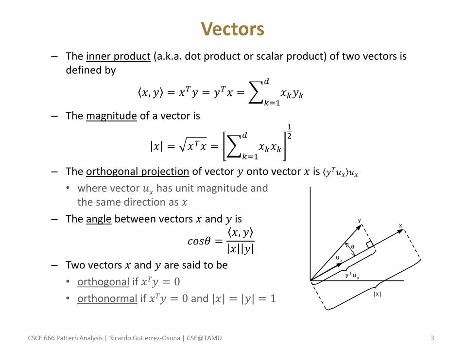
Vectors – The inner product (a.k.a. dot product or scalar product) of two vectors is

defined by

𝑥, 𝑦 = 𝑥𝑇𝑦 = 𝑦𝑇𝑥 = 𝑥𝑘𝑦𝑘𝑑

𝑘=1

– The magnitude of a vector is

𝑥 = 𝑥𝑇𝑥 = 𝑥𝑘𝑥𝑘𝑑

𝑘=1

12

– The orthogonal projection of vector 𝑦 onto vector 𝑥 is 𝑦𝑇𝑢𝑥 𝑢𝑥

• where vector 𝑢𝑥 has unit magnitude and the same direction as 𝑥

– The angle between vectors 𝑥 and 𝑦 is

𝑐𝑜𝑠𝜃 =𝑥, 𝑦

𝑥 𝑦

– Two vectors 𝑥 and 𝑦 are said to be

• orthogonal if 𝑥𝑇𝑦 = 0

• orthonormal if 𝑥𝑇𝑦 = 0 and |𝑥| = |𝑦| = 1

yx

ux

|x |

y T ux


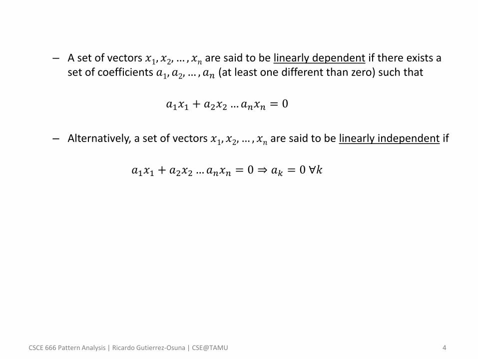
– A set of vectors 𝑥1, 𝑥2, … , 𝑥𝑛 are said to be linearly dependent if there exists a set of coefficients 𝑎1, 𝑎2, … , 𝑎𝑛 (at least one different than zero) such that

𝑎1𝑥1 + 𝑎2𝑥2…𝑎𝑛𝑥𝑛 = 0

– Alternatively, a set of vectors 𝑥1, 𝑥2, … , 𝑥𝑛 are said to be linearly independent if

𝑎1𝑥1 + 𝑎2𝑥2…𝑎𝑛𝑥𝑛 = 0 ⇒ 𝑎𝑘 = 0 ∀𝑘


Matrices – The determinant of a square matrix 𝐴𝑑𝑑 is

𝐴 = 𝑎𝑖𝑘 𝐴𝑖𝑘 −1𝑘+𝑖

𝑑

𝑘=1

• where 𝐴𝑖𝑘 is the minor formed by removing the ith row and the kth column of 𝐴

• NOTE: the determinant of a square matrix and its transpose is the same: |𝐴| = |𝐴𝑇|

– The trace of a square matrix 𝐴𝑑𝑑 is the sum of its diagonal elements

𝑡𝑟 𝐴 = 𝑎𝑘𝑘

𝑑

𝑘=1

– The rank of a matrix is the number of linearly independent rows (or columns)

– A square matrix is said to be non-singular if and only if its rank equals the number of rows (or columns)

• A non-singular matrix has a non-zero determinant


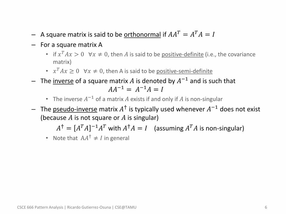
– A square matrix is said to be orthonormal if 𝐴𝐴𝑇 = 𝐴𝑇𝐴 = 𝐼

– For a square matrix A

• if 𝑥𝑇𝐴𝑥 > 0 ∀𝑥 ≠ 0, then 𝐴 is said to be positive-definite (i.e., the covariance matrix)

• 𝑥𝑇𝐴𝑥 ≥ 0 ∀𝑥 ≠ 0, then A is said to be positive-semi-definite

– The inverse of a square matrix 𝐴 is denoted by 𝐴−1 and is such that 𝐴𝐴−1 = 𝐴−1𝐴 = 𝐼

• The inverse 𝐴−1 of a matrix 𝐴 exists if and only if 𝐴 is non-singular

– The pseudo-inverse matrix 𝐴† is typically used whenever 𝐴−1 does not exist (because 𝐴 is not square or 𝐴 is singular)

𝐴† = 𝐴𝑇𝐴 −1𝐴𝑇 with 𝐴†𝐴 = 𝐼 (assuming 𝐴𝑇𝐴 is non-singular)

• Note that A𝐴† ≠ 𝐼 in general


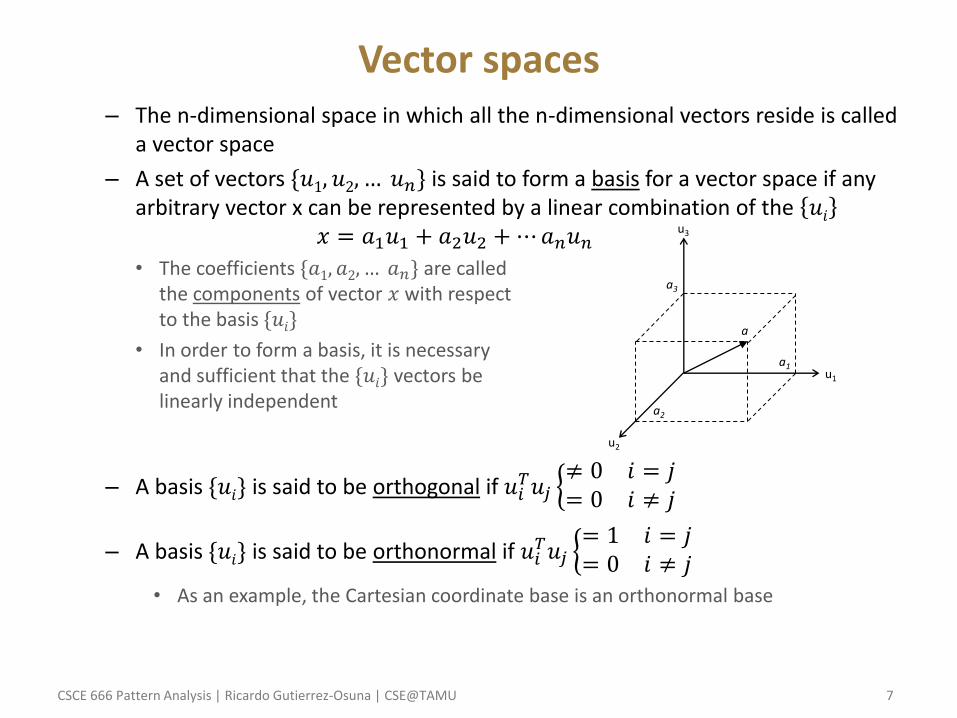
Vector spaces – The n-dimensional space in which all the n-dimensional vectors reside is called

a vector space

– A set of vectors {𝑢1, 𝑢2, … 𝑢𝑛} is said to form a basis for a vector space if any arbitrary vector x can be represented by a linear combination of the 𝑢𝑖

𝑥 = 𝑎1𝑢1 + 𝑎2𝑢2 +⋯𝑎𝑛𝑢𝑛

• The coefficients {𝑎1, 𝑎2, … 𝑎𝑛} are called the components of vector 𝑥 with respect to the basis {𝑢𝑖}

• In order to form a basis, it is necessary and sufficient that the {𝑢𝑖} vectors be linearly independent

– A basis {𝑢𝑖} is said to be orthogonal if 𝑢𝑖𝑇𝑢𝑗 ≠ 0 𝑖 = 𝑗= 0 𝑖 ≠ 𝑗

– A basis {𝑢𝑖} is said to be orthonormal if 𝑢𝑖𝑇𝑢𝑗 = 1 𝑖 = 𝑗= 0 𝑖 ≠ 𝑗

• As an example, the Cartesian coordinate base is an orthonormal base

u2

u1

u3

a1

a2

a3

a


– Given n linearly independent vectors {𝑥1, 𝑥2, … 𝑥𝑛}, we can construct an orthonormal base 𝜙1, 𝜙2, …𝜙𝑛 for the vector space spanned by {𝑥𝑖} with the Gram-Schmidt orthonormalization procedure (to be discussed in the RBF lecture)

– The distance between two points in a vector space is defined as the magnitude of the vector difference between the points

𝑑𝐸 𝑥, 𝑦 = 𝑥 − 𝑦 = 𝑥𝑘 − 𝑦𝑘2

𝑑

𝑘=1

12

• This is also called the Euclidean distance


Linear transformations – A linear transformation is a mapping from a vector space 𝑋𝑁 onto a vector

space 𝑌𝑀, and is represented by a matrix • Given vector 𝑥𝜖𝑋𝑁, the corresponding vector y on 𝑌𝑀 is computed as

𝑦1𝑦2⋮𝑦𝑀

=

𝑎11 𝑎12 𝑎1𝑁𝑎21 𝑎22 𝑎2𝑁

⋱𝑎𝑀1 𝑎𝑀2 𝑎𝑀𝑁

𝑥1𝑥2⋮𝑥𝑁

• Notice that the dimensionality of the two spaces does not need to be the same

• For pattern recognition we typically have 𝑀 < 𝑁 (project onto a lower-dim space)

– A linear transformation represented by a square matrix A is said to be orthonormal when 𝐴𝐴𝑇 = 𝐴𝑇𝐴 = 𝐼 • This implies that 𝐴𝑇 = 𝐴−1

• An orthonormal xform has the property of preserving the magnitude of the vectors

𝑦 = 𝑦𝑇𝑦 = 𝐴𝑥 𝑇𝐴𝑥 = 𝑥𝑇𝐴𝑇𝐴𝑥 = 𝑥𝑇𝑥 = 𝑥

• An orthonormal matrix can be thought of as a rotation of the reference frame

• The row vectors of an orthonormal xform are a set of orthonormal basis vectors

𝑌𝑀×1 =

← 𝑎1→← 𝑎2→

← 𝑎𝑁→

𝑋𝑁×1 with 𝑎𝑖𝑇𝑎𝑗 =

0 𝑖 ≠ 𝑗1 𝑖 = 𝑗


Eigenvectors and eigenvalues – Given a matrix 𝐴𝑁×𝑁, we say that 𝑣 is an eigenvector* if there exists a scalar 𝜆

(the eigenvalue) such that 𝐴𝑣 = 𝜆𝑣

– Computing the eigenvalues

𝐴𝑣 = 𝜆𝑣 ⇒ 𝐴 − 𝜆𝐼 𝑣 = 0 ⇒ 𝑣 = 0 𝐴 − 𝜆𝐼 = 0

𝐴 − 𝜆𝐼 = 0 ⇒ 𝐴 − 𝜆𝐼 = 0 ⇒ 𝜆𝑁 + 𝑎1𝜆𝑁−1 + 𝑎2𝜆

𝑁−2 + +𝑎𝑁−1𝜆 + 𝑎0 = 0

Characteristic equation

*The "eigen-" in "eigenvector" translates as "characteristic"

Trivial solution Non-trivial solution


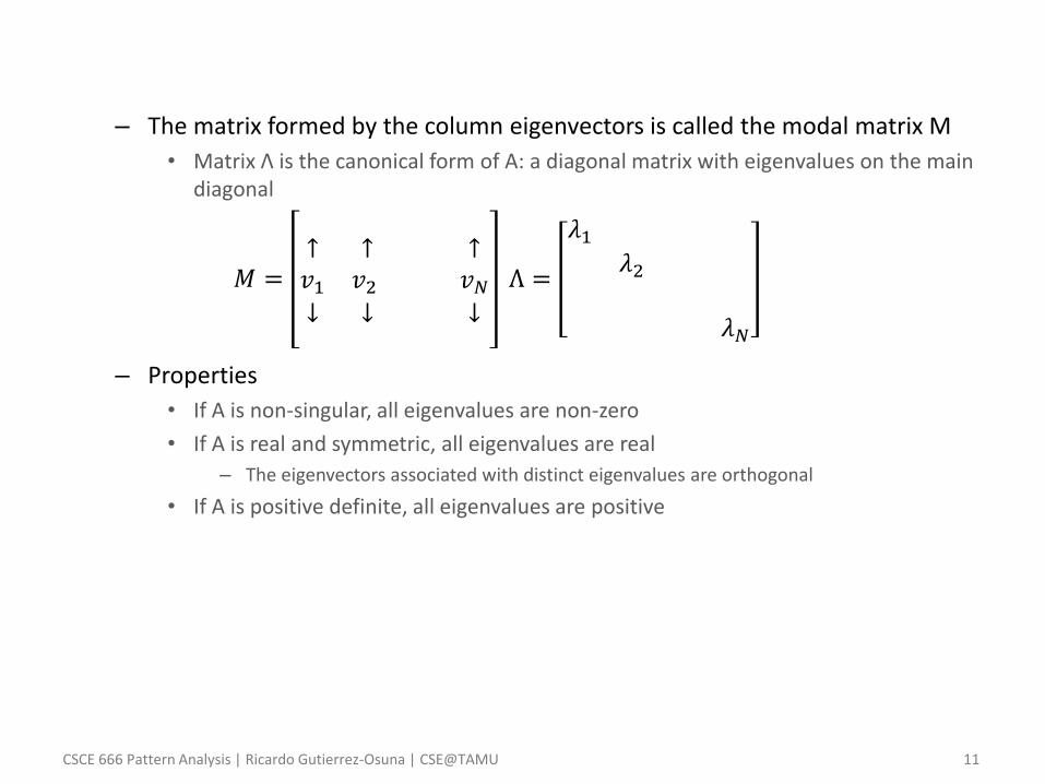
– The matrix formed by the column eigenvectors is called the modal matrix M

• Matrix Λ is the canonical form of A: a diagonal matrix with eigenvalues on the main diagonal

𝑀 =↑ ↑ ↑𝑣1 𝑣2 𝑣𝑁↓ ↓ ↓

Λ =

𝜆1𝜆2

𝜆𝑁

– Properties

• If A is non-singular, all eigenvalues are non-zero

• If A is real and symmetric, all eigenvalues are real

– The eigenvectors associated with distinct eigenvalues are orthogonal

• If A is positive definite, all eigenvalues are positive


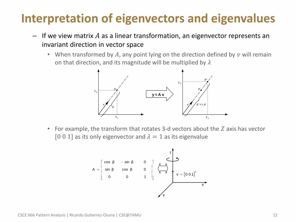
Interpretation of eigenvectors and eigenvalues – If we view matrix 𝐴 as a linear transformation, an eigenvector represents an

invariant direction in vector space

• When transformed by 𝐴, any point lying on the direction defined by 𝑣 will remain on that direction, and its magnitude will be multiplied by 𝜆

• For example, the transform that rotates 3-d vectors about the 𝑍 axis has vector [0 0 1] as its only eigenvector and 𝜆 = 1 as its eigenvalue

x1

x2

v

P

d

y1

y2

v

P

d ’= d

P ’

y = A x

x

y

z

T

100v

100

0βcosβsin

0βsinβcos

A


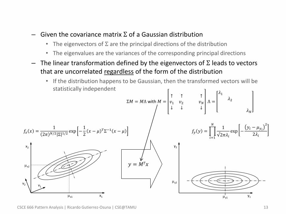
– Given the covariance matrix Σ of a Gaussian distribution

• The eigenvectors of Σ are the principal directions of the distribution

• The eigenvalues are the variances of the corresponding principal directions

– The linear transformation defined by the eigenvectors of Σ leads to vectors that are uncorrelated regardless of the form of the distribution

• If the distribution happens to be Gaussian, then the transformed vectors will be statistically independent

y1

y2

y1

y2

x1

x2

v1 v2

x1

x2 𝑦 = 𝑀𝑇𝑥

Σ𝑀 = 𝑀Λ with 𝑀 =↑ ↑ ↑𝑣1 𝑣2 𝑣𝑁↓ ↓ ↓

Λ =

𝜆1𝜆2

𝜆𝑁

𝑓𝑥 𝑥 =1

2𝜋 𝑁/2 Σ 1/2exp −1

2𝑥 − 𝜇 𝑇Σ−1 𝑥 − 𝜇 𝑓𝑦 𝑦 =

1

√2𝜋𝜆𝑖exp −

𝑦𝑖 − 𝜇𝑦𝑖2

2𝜆𝑖

𝑁

𝑖=1


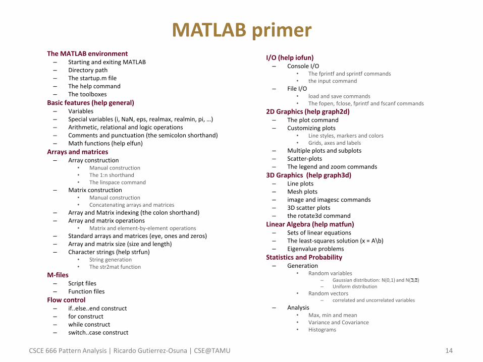
MATLAB primer • The MATLAB environment

– Starting and exiting MATLAB – Directory path – The startup.m file – The help command – The toolboxes

• Basic features (help general) – Variables – Special variables (i, NaN, eps, realmax, realmin, pi, …) – Arithmetic, relational and logic operations – Comments and punctuation (the semicolon shorthand) – Math functions (help elfun)

• Arrays and matrices – Array construction

• Manual construction • The 1:n shorthand • The linspace command

– Matrix construction • Manual construction • Concatenating arrays and matrices

– Array and Matrix indexing (the colon shorthand) – Array and matrix operations

• Matrix and element-by-element operations

– Standard arrays and matrices (eye, ones and zeros) – Array and matrix size (size and length) – Character strings (help strfun)

• String generation • The str2mat function

• M-files – Script files – Function files

• Flow control – if..else..end construct – for construct – while construct – switch..case construct

• I/O (help iofun) – Console I/O

• The fprintf and sprintf commands • the input command

– File I/O • load and save commands • The fopen, fclose, fprintf and fscanf commands

• 2D Graphics (help graph2d) – The plot command – Customizing plots

• Line styles, markers and colors • Grids, axes and labels

– Multiple plots and subplots – Scatter-plots – The legend and zoom commands

• 3D Graphics (help graph3d) – Line plots – Mesh plots – image and imagesc commands – 3D scatter plots – the rotate3d command

• Linear Algebra (help matfun) – Sets of linear equations – The least-squares solution (x = A\b) – Eigenvalue problems

• Statistics and Probability – Generation

• Random variables – Gaussian distribution: N(0,1) and N( , ) – Uniform distribution

• Random vectors – correlated and uncorrelated variables

– Analysis • Max, min and mean • Variance and Covariance • Histograms

l3: review of linear algebra and matlabcourses.cs.tamu.edu/rgutier/csce666_f16/l3.pdf · l3: review...

Documents