l14: refinements for hmms - courses.cs.tamu.educourses.cs.tamu.edu/rgutier/csce689_s11/l14.pdf ·...

Introduction to Speech Processing | Ricardo Gutierrez-Osuna | CSE@TAMU 1

L14: Refinements for HMMs

• Types of HMM structures

• Implementation issues

• Continuous and semi-continuous HMMs

• Robustness to environment and channel effects

• Speaker independent recognition

• Model adaptation

• Discriminative training

This lecture is based on [Rabiner and Juang, 1993; Holmes, 2001, ch11; Gold and Morgan, 200, ch.27]


Types of HMM structure

• Ergodic – An ergodic HMM is a fully connected model,

where each state can be reached in one step from every other state

• This is the most general type of HMM, and the one that had been implicitly assumed earlier

• Left-right – A left-right or Bakis model is one where no transitions are allowed to

states whose indices are lower than the current state 𝑎𝑖𝑗 = 0; ∀𝑗 < 𝑖

• Left-right models are best suited to model signals whose properties change over time, such as speech

• When using left-right models, some additional constraints are commonly placed, such as preventing large transitions 𝑎𝑖𝑗 = 0 ∀𝑗 > 𝑖 + Δ

[Rabiner, 1989]


Implementation issues

• Scaling – Since 𝛼𝑡 𝑖 is the product of a large number of terms that are less

than one, machine precision is likely to be exceeded sooner or later

– To solve this problem, the 𝛼′𝑠 are re-scaled periodically to avoid underflow, and a similar scaling is done to the 𝛽′𝑠 so that the scaling coefficients cancel out exactly

• Multiple observation sequences – Our HMM derivations were based on a single observation sequence

• This becomes a problem in left-right models, since the transient nature of the states only allows a few observations to be used for each state

– For this reason, one has to use multiple observation sequences • Re-estimation formulas for multiple sequences can be found in [Rabiner

and Juang, 1993]


• Initial parameter estimates – How are the initial HMM parameters chosen so that Baum-Welch is

more likely to converge to a global maximum?

– Random or uniform initial values for and 𝐴 have experimentally been found to work well in most cases

– Careful selection of initial values for 𝐵, however, has been found to be helpful in the discrete case and essential in the continuous case • These initial estimates may be found by segmenting the sequences with k-

means clustering


Continuous and semi-continuous HMMs

• Discrete HMMs – Our discussion of HMMs thus far has focused on discrete HMMs

– Discrete HMMs assume that the observations are defined by a set of discrete symbols from a finite alphabet

– In speech, however, observations are inherently multidimensional and have continuous features

• There are two alternatives to handle continuous vectors – Convert the continuous multivariate observations into discrete

univariate observations via a codebook (e.g., with k-means)

• This approach, however, may lead to degraded performance as a result of the discretization of the continuous signals

– Employ HMM states that have continuous observation densities 𝑏𝑗

• This is, in general, a much better alternative, which we explore next


• Continuous HMMs – C-HMMs model the observation probabilities with a continuous

density function, as opposed to a multinomial

• To ensure that the model parameters can be re-estimated in a consistent manner, some restrictions are applied to the form of the observation pdf

• The most common form is the Gaussian mixture model

𝑏𝑗 𝑜 = 𝑐𝑗𝑘𝑁 𝑜, 𝜇𝑗𝑘 , Σ𝑗𝑘𝑀

𝑘=1

• where 𝑜 is the observation vector, and 𝑐𝑗𝑘 , 𝜇𝑗𝑘 , Σ𝑗𝑘 are the mixture

coefficient, mean and covariance for the 𝑘-th Gaussian component at state 𝑆𝑗, respectively


– The re-estimation formulas for the continuous case generalize very gracefully from the discrete HMM

• The term 𝛾𝑡 𝑗 generalizes to 𝛾𝑡 𝑗, 𝑘 , which represents the probability of being in state 𝑆𝑗 at time 𝑡 with 𝑘-mixture component accounting for

observation 𝑜𝑡

𝛾𝑡 𝑗, 𝑘 =𝛼𝑡 𝑗 𝛽𝑡 𝑗

𝛼𝑡 𝑗 𝛽𝑡 𝑗𝑁𝑗=1

𝑐𝑗𝑘𝑁 𝑜𝑡,𝜇𝑗𝑘,Σ𝑗𝑘

𝑐𝑗𝑚𝑁 𝑜𝑡,𝜇𝑗𝑚,Σ𝑗𝑚𝑀𝑚=1

• Note how the first fraction is the same as in the discrete HMM case, whereas the second fraction is due to the 𝑘-th Gaussian component


– The re-estimation formulas for the continuous HMM are

• The new 𝑐 𝑗𝑘is the ratio between the expected number of times the

system is in state 𝑆𝑗 using the 𝑘-th mixture component, and the expected number of times the system is in state 𝑆𝑗

𝑐 𝑗𝑘 = 𝛾𝑡 𝑗,𝑘𝑇

𝑡=1

𝛾𝑡 𝑗,𝑘𝑀𝑘=1

𝑇𝑡=1

• The new 𝜇 𝑗𝑘 weights the numerator in the equation for 𝑐 𝑗𝑘 by the

observation, to produce the portion of the observation that can be accounted by that mixture component

𝜇 𝑗𝑘 = 𝛾𝑡 𝑗,𝑘 𝑜𝑡

𝑇𝑡=1

𝛾𝑡 𝑗,𝑘𝑇𝑡=1

• The re-estimation formula for the covariance term can be interpreted similarly

Σ 𝑗𝑘 = 𝛾𝑡 𝑗,𝑘 𝑜𝑡−𝜇𝑗𝑘 𝑜𝑡−𝜇𝑗𝑘

𝑇𝑇𝑡=1

𝛾𝑡 𝑗,𝑘𝑇𝑡=1

• The re-estimation formula for transition probabilities 𝑎𝑖𝑗 is the same as in

the discrete HMM


• Issues with C-HMMs – C-HMMs avoid the distortions introduced by a discrete codebook, but

• A large number of mixtures are generally required to improve the recognition accuracy as compared to D-HMMs [Huang, 1992]

• As a result, the computational complexity of C-HMMs increases considerably with respect to D-HMMs

• The number of free parameters increases significantly, which means that a larger training set is required to train the model properly

• Semi-continuous HMMs – SC-HMMs represent a compromise between D-HMMs and C-HMMs

– In SC-HMMs, the observation space is modeled with a Gaussian mixture whose components 𝜇, Σ are shared by all states in the HMM

– Each state in the HMM, though, is allowed to have a different mixing coefficient 𝑐𝑗𝑘 for each of the 𝑘 Gaussian components in the “common” mixture

– SC-HMMs are also referred to as tied-mixture HMMs


Robustness to environmental & channel effects

• ASR in real environments – Ideally, speech signals for ASR would be recorded in a quiet

environment, with a good-quality close-talking microphone

– In practice, the speech signal will have been corrupted in some way • Even if the recorded signal isn’t corrupted, speakers tend to modify their

speech (e.g., increased vocal effort) as the environment worsens; this is known as the Lombard effect

• Types of noise – Additive noise

• Examples: environmental noise (electronics, machinery, vehicles, other speakers), noise introduced by poor-quality microphones or noisy transmission channels

• Additive noise is best dealt within the linear spectral domain

– Convolutional noise • Examples: room reverberation, differences in microphone handsets

(channel bandwidth limitations, spectral shaping)

• Convolutional noise is best dealt within the log spectral or cepstral domain, since it becomes additive


– These and other sources of distortion create a mismatch between the conditions in which the recognizer is used, and those under which is was initially trained

• One possible solution to this issue is to train the recognizer under similar conditions as those that will occur operationally

• However, it is not always possible to predict operational conditions in advance, and these conditions change over time

– Thus, techniques are needed to deal with corrupted speech signals, which can be grouped into two categories

• Feature-based methods

– Applied directly at the level of speech features

• Model-based methods

– Built into the recognition process itself


• Feature-based methods – Spectral subtraction

• Used to remove additive noise

• An average of the noise spectrum is obtained from silent segments

• This average noise spectrum is subtracted from the speech spectrum

• Negative values in the resulting spectrum are set to zero

– Cepstral mean subtraction/normalization • Used to remove convolutional noise

• Noise spectra must be estimated in speech regions, since speech must be present for convolutional distortions to appear

• Assuming these distortions remain constant over an utterance, one can then remove them by subtracting the (cepstral or log) mean feature vector computed over a long window

– Relative spectral processing (RASTA) • Removes slowly varying components in the spectrum, to which human

listeners do not pay much attention

• Generally performed with Perceptual Linear Prediction (PLP), a variant of LPC that is more consistent with psychoacoustics


• Model-based methods – Noise masking

• A simple technique that replaces any channel levels below noise levels with an estimate of the noise signal

• By applying this to both observed signals and to the stored model, noisy channels do not contribute to the model’s predictions

– Decomposition

• A separate HMM is built to model noise characteristics

– A one-state HMM may suffice for stationary noise, multi-state may be needed for more complex noise sources

• For each possible state pairing (one state from the noise HMM, another from the speech HMM), estimate probability that signal belongs either to noise or to speech

– As a result, the method can be used to decompose a noisy speech signal into its constituent parts


– Parallel Model Combination

• Separate HMMs are built for both clean speech and pure noise, using standard cepstral methods

• State parameters are then converted into linear spectra (i.e., by means of an inverse DCT) and added for different levels of noise

• The added parameters are converted back to the cepstral domain to obtain an HMM that handles ‘corrupted’ speech

[Holmes, 2001]


Speaker-independent recognition

• Speaker differences – Acoustic realizations of a word may be highly variable across speakers

due to physical differences, accent/dialect, speaking style, etc.

– One alternative is to train the recognizer on multiple speakers

• The underlying Gaussians become broader to accommodate for multiple speakers and therefore will have a greater degree of overlap across different phonemes, which impacts performance

– A second option is to train a separate recognizer for each type of speaker (e.g., males vs. females)

• With this option, however, we either need to identify the type of the speaker (which cannot be done with perfect accuracy) or run multiple recognizers in parallel (which increases computational load)

– Other alternatives, which we review next, include

• Speaker normalization

• Model adaptation


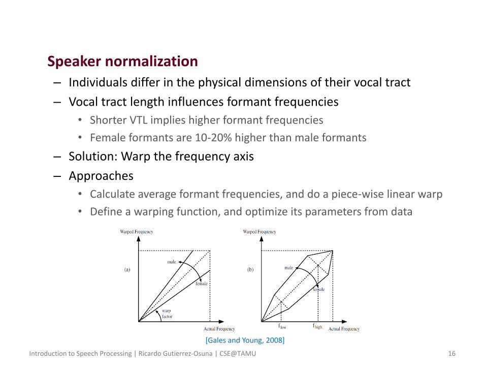
• Speaker normalization – Individuals differ in the physical dimensions of their vocal tract

– Vocal tract length influences formant frequencies

• Shorter VTL implies higher formant frequencies

• Female formants are 10-20% higher than male formants

– Solution: Warp the frequency axis

– Approaches

• Calculate average formant frequencies, and do a piece-wise linear warp

• Define a warping function, and optimize its parameters from data

[Gales and Young, 2008]


Model adaptation

• Objective – Adapts model parameters to provide a better match to data from

other speaker, channel effects or recording conditions

– The amount of calibration data needed to adapt model parameters is only a fraction of that required to train a recognizer from scratch

– Thus, adaptation provides a trade-off between two types of recognizer • Speaker-dependent (SD) recognizers: trained on data from a single

speaker, easier to train and more accurate

• Speaker-independent (SI) recognizers, trained on data from multiple speakers, longer training time, lower recognition accuracy

• Types of model adaptation – Supervised: the text of the adaptation is known

– Unsupervised: the text of the adaptation is unknown • In this case, the initial model is used to recognize the calibration data, and

the recognized transcription is then used to adapt the models

• As would be expected, this method requires that the initial recognition be sufficiently accurate


• Maximum likelihood linear regression (MLLR) – The most widely used of speaker adaptation

– Applies a linear transformation to the mean of the Gaussians

𝜇 𝑗𝑚=𝐴𝑐𝜇𝑗𝑚 + 𝑏𝑐

• where 𝐴𝑐 and 𝑏𝑐 are a regression matrix and bias vector associated with a broad class 𝑐, which are learned using an EM procedure

– When the amount of adaptation data is very small, a single transform 𝑐 = 1 can be shared across all the Gaussians in the model; as the

amount of data increases, the number of transforms can be increased accordingly

– Using a small amount of adaptation data (15 sec), MLLR can improve recognition performance by 7-10% • MLLR can also be applied to the covariance matrices, though the additional

gains in performance are modest (less than 2%)

– A variant of MLLR known as constrained MLLR (CMLLR) applies a common linear transform to the mean and covariance

𝜇 𝑗𝑚=𝐴𝑐𝜇𝑗𝑚 + 𝑏𝑐

Σ 𝑗𝑚 = 𝐴𝑐Σ𝑗𝑚𝐴𝑐𝑇


• Bayesian/MAP adaptation – Uses parameters from an existing SI recognizer as priors, and attempts

to maximize the parameter’s posterior given the new calibration data 𝜃𝑀𝐴𝑃 = arg max

𝜃𝑃 𝑋 𝜃 𝑃 𝜃

– Using various assumptions, MAP adaptation reduces to simple expressions for updating the Gaussian means (𝑗: state; 𝑚: mixture)

𝜇 𝑗𝑚 =𝑁𝑗𝑚

𝑁𝑗𝑚 + 𝜏𝜇 𝑗𝑚 +

𝜏

𝑁𝑗𝑚 + 𝜏𝜇𝑗𝑚

• where 𝜇𝑗𝑚 and 𝜇 𝑗𝑚 are the mean of the SI model and the mean of the

adaptation data, respectively, 𝑁𝑗𝑚 is the occupation likelihood of the

adaptation data and 𝜏 is a weighting for the a-priori knowledge

• Similar equations can be derived for the covariance parameters Σ𝑗𝑚

– Thus, the MAP remains close to the SI estimate when 𝑁𝑗𝑚 is small, and

departs as the amount of adaptation data increases

– MAP has more degrees of freedom than MLLR but also requires significantly more adaptation data


• Speaker adaptive training (SAT) – MLLR can be incorporated into the training procedure of speaker-

independent recognizers

– Procedure

• Start off with a default SI recognizer

• Estimate a transform for each speaker

• Re-estimate the model given each of the speakers transformed data

• Repeat until convergence or termination condition is met

– As a result, the final SI recognizer is less influenced by speaker-specific characteristics, since these are captured by the transforms

– SAT can reduce error rates by an additional 5-10% w.r.t. to MLLR


Discriminative training

• Drawbacks of MLE estimation – MLE maximizes the likelihood of the data given the correct model 𝜔𝑖,

and only data from class 𝜔𝑖 is used to train the parameters 𝜃𝑖

• However, there is no guarantee that if 𝑥 ∈ 𝜔𝑖, the likelihood 𝑃 𝑥|𝜔𝑖 will

be higher than that of the wrong classes 𝑃 𝑥|𝜔𝑗 𝑗≠𝑖

– In contrast, discriminative training techniques aim to maximize the ability of the model to distinguish among the different classes

• This is achieved by estimating model parameters in a way that improves the likelihood of the correct model relative to the likelihood of the incorrect models

– Three discriminative training techniques will be reviewed here

• Maximum mutual information (MMI) training

• Corrective training

• Generalized probabilistic descent (GPD)


• Maximum mutual information (MMI) training – The goal of MMI training is to maximize the mutual information between

the observations 𝑥 and the class labels 𝜔

𝐼 𝑥, 𝜔|𝜃 = 𝐸 log𝑝 𝑥,𝜔|𝜃

𝑝 𝑥|𝜃 𝑃 𝜔|𝜃

• Which, for a particular choice of model and acoustic pair, becomes

𝐼 𝑥, 𝜔𝑖|𝜃 = log𝑝 𝑥, 𝜔𝑖 𝜃

𝑝 𝑥 𝜃 𝑃 𝜔𝑖 𝜃

– To see that this criterion is discriminative, note that 𝑝 𝑥, 𝜔𝑖|𝜃 = 𝑝 𝑥|𝜔𝑖 , 𝜃 𝑃 𝜔𝑖|𝜃

• Thus, substituting back into the earlier expression yields

𝐼 𝑥, 𝜔𝑖|𝜃 = log𝑝 𝑥|𝜔𝑖 , 𝜃

𝑝 𝑥|𝜃

• Assuming that we have a total of 𝐶 models, then

𝐼 𝑥, 𝜔𝑖|𝜃 = log𝑝 𝑥|𝜔𝑖 , 𝜃

𝑝 𝑥|𝜔𝑐 , 𝜃 𝑃 𝜔𝑐|𝜃𝐶𝑐=1

• Note that this equation differs from the one in the previous page in that it lacks a prior in the numerator and there is a log function

– Gradient descent techniques are used to update parameters in the direction that most increases the mutual information


• Corrective training – A pragmatic discriminative training procedure, in which the

parameters are modified only for those utterances in which the correct model had a lower likelihood than the best model

– For these cases, the acoustic probabilities are adapted upward (towards the example) for the correct model 𝜔𝑐 and downwards for the incorrect models 𝜔𝑖:

• if 𝑝 𝑥|𝜔𝑖 , 𝜃 ≥ 𝑝 𝑥|𝜔𝑐 , 𝜃 + Δ

• then 𝜃 → 𝜃∗

• such that 𝑝 𝑥|𝜔𝑐 , 𝜃∗ ≥ 𝑝 𝑥|𝜔𝑐, 𝜃 and 𝑝 𝑥|𝜔𝑖 , 𝜃

∗ ≤ 𝑝 𝑥|𝜔𝑖 , 𝜃

– where Δ is a margin that must be exceeded before an utterance is considered to be recognized so poorly as to suggest correction of the models

• For more details, see [LR Bahl, PF Brown, PV de Souza, and RL Mercer, “A New Algorithm for the Estimation of Hidden Markov Model Parameters,” ICASSP, 1988, p. 493-496]


• Generalized probabilistic descent – GPD is a generalization of corrective training, MMI as well as several

other discriminative procedures

– Consider a discriminant function 𝑔𝑖 𝑥; 𝜃 for each class 𝜔𝑖 𝑔𝑖 𝑥|𝜃 = − log 𝑝 𝑥|𝜔𝑖 , 𝜃

– In GDP, we define the following miss-classification measure

𝑑𝑗 𝑥|𝜃 = 𝑔𝑗 𝑥|𝜃 − log1

𝐶−1 𝑒𝜂𝑔𝑘 𝑥|𝜃

𝑘≠𝑗

1/𝜂

• where the term 𝜂 allows us to control the effect of the competing classes

– For 𝜂 = 1, the competing term is the average of all competing discriminant functions, whereas for 𝜂 → ∞ the competing term is the maximum of them

– Note that, for 𝜂 = 1 and 𝑃 𝜔𝑖 = 1/𝐶, this measure reduces to that of MMI

– This measure can be used to minimize the misclassification rate

• This is done by passing 𝑑𝑖 𝑥; 𝜃 through a sigmoidal function 𝑆 and minimizing the following expression through gradient descent

𝐸 𝜃 = 𝑆 𝑑𝑖 𝑥; 𝜃𝑥∈𝜔𝑗𝑗


• Discussion – MMI and GPD are much more computationally intensive than MLE due

to the inefficiency of gradient descent and the fact that every model parameter must be updated for each training example

– As a result, these procedures are generally used only for tasks containing few classes or data samples

– For all other cases, corrective training provides a more pragmatic approach to discriminative training

l14: refinements for hmms - courses.cs.tamu.educourses.cs.tamu.edu/rgutier/csce689_s11/l14.pdf ·...

Documents