L1 ADAPTIVE CONTROL AUGMENTATION SYSTEMFOR THE X-48B AIRCRAFT

BY

TYLER JOHN LEMAN

THESIS

Submitted in partial fulfillment of the requirementsfor the degree of Master of Science in Mechanical Engineering

in the Graduate College of theUniversity of Illinois at Urbana-Champaign, 2009

Urbana, Illinois

Advisers:

Professor Naira HovakimyanProfessor Geir E. Dullerud

Abstract

This thesis considers the application of L1 adaptive control methodology to

a model of the X-48B Blended Wing Body aircraft. We explicitly verify the

performance bounds of the adaptive flight control system at various flight

conditions. We demonstrate that the resulting L1 adaptive controller does

not require tuning or redesign from one flight condition to another. Further-

more, once designed according to the theoretical guidelines, the L1 adaptive

controller ensures uniform transient and steady-state performance across the

entire flight envelope in the presence of significantly coupled dynamics and

control surface failures.

ii

Acknowledgements

I would like to sincerely thank my advisers, Professor Naira Hovakimyan

and Professor Geir Dullerud, for giving me the opportunity to work on this

project and investing their time in my education. I also want to thank

Enric Xargay, who spent many hours helping me understand L1 theory and

implementation. Thank you to Evgeny Kharisov for his help formatting this

thesis. And finally, a big thank you to Rachel and my parents for their

constant support.

iii

Contents

1 Introduction . . . . . . . . . . . . . . . . . . . . . . . . . . . . 1

1.1 Background and Motivation . . . . . . . . . . . . . . . . . . . 1

1.2 L1 Adaptive Control Overview . . . . . . . . . . . . . . . . . . 3

1.3 X-48B Blended Wing Body . . . . . . . . . . . . . . . . . . . 5

1.4 Organization of Thesis . . . . . . . . . . . . . . . . . . . . . . 6

2 Theoretical Framework . . . . . . . . . . . . . . . . . . . . . 7

2.1 Baseline Control Architecture . . . . . . . . . . . . . . . . . . 7

2.2 Problem Formulation . . . . . . . . . . . . . . . . . . . . . . . 10

2.3 L1 Adaptive Controller Formulation . . . . . . . . . . . . . . . 13

3 Simulation Results . . . . . . . . . . . . . . . . . . . . . . . . 17

3.1 Remarks on the Implementation . . . . . . . . . . . . . . . . . 17

3.2 Results at Stall AOA Trim . . . . . . . . . . . . . . . . . . . . 21

3.3 Results at Normal Flight AOA Trim . . . . . . . . . . . . . . 23

3.4 Time Delay Margin . . . . . . . . . . . . . . . . . . . . . . . . 28

3.5 Comparison of Virtual Control Commands . . . . . . . . . . . 33

iv

4 Conclusions and Future Work . . . . . . . . . . . . . . . . . 36

References . . . . . . . . . . . . . . . . . . . . . . . . . . . . . . . 38

v

Chapter 1

Introduction

1.1 Background and Motivation1

Aircraft loss of control (LOC) during flight is a leading cause of fatal aviation

accidents [2]. Loss of control can result from any number of factors, includ-

ing system and component failures, control system impairment or damage,

inclement weather, or inappropriate pilot inputs. In general, a loss of control

accident takes the airplane beyond the normal flight envelope into regions

where aerodynamic data is not available from conventional sources. For ex-

ample, wind tunnel test data for aerodynamic forces and moments at high

angles of attack is limited in accuracy, as is modeling the effect of a control

surface failure on the aircraft’s dynamics. Thus, the aerodynamic changes

due to such failures cannot be predicted a priori.

1Much of the work contained in this thesis has been previously published in Reference [1]and is reprinted with permission.

1

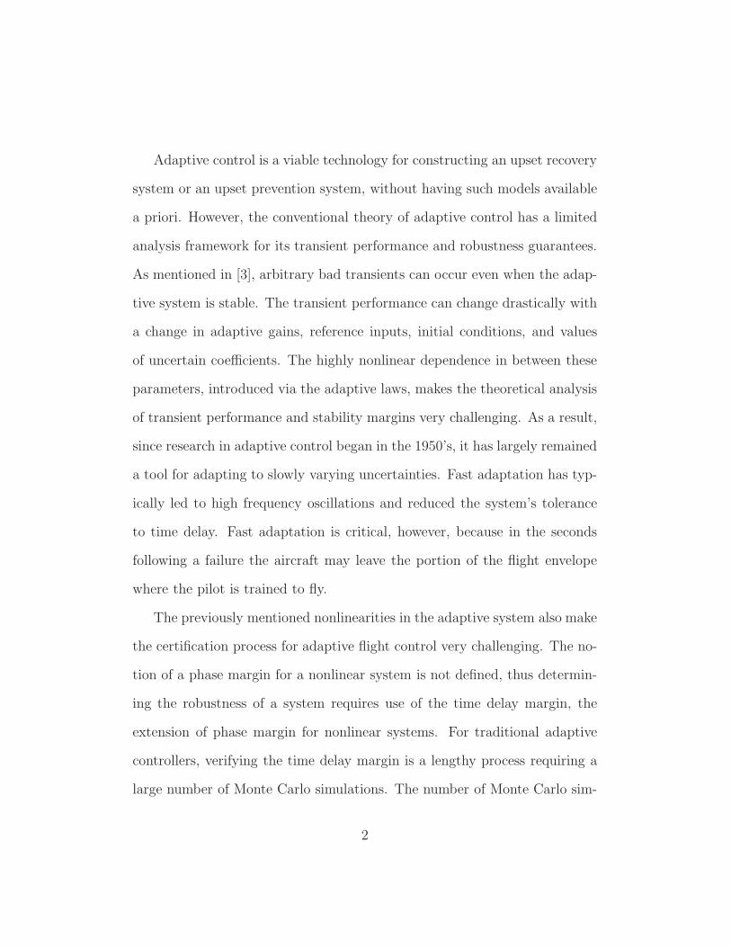
Adaptive control is a viable technology for constructing an upset recovery

system or an upset prevention system, without having such models available

a priori. However, the conventional theory of adaptive control has a limited

analysis framework for its transient performance and robustness guarantees.

As mentioned in [3], arbitrary bad transients can occur even when the adap-

tive system is stable. The transient performance can change drastically with

a change in adaptive gains, reference inputs, initial conditions, and values

of uncertain coefficients. The highly nonlinear dependence in between these

parameters, introduced via the adaptive laws, makes the theoretical analysis

of transient performance and stability margins very challenging. As a result,

since research in adaptive control began in the 1950’s, it has largely remained

a tool for adapting to slowly varying uncertainties. Fast adaptation has typ-

ically led to high frequency oscillations and reduced the system’s tolerance

to time delay. Fast adaptation is critical, however, because in the seconds

following a failure the aircraft may leave the portion of the flight envelope

where the pilot is trained to fly.

The previously mentioned nonlinearities in the adaptive system also make

the certification process for adaptive flight control very challenging. The no-

tion of a phase margin for a nonlinear system is not defined, thus determin-

ing the robustness of a system requires use of the time delay margin, the

extension of phase margin for nonlinear systems. For traditional adaptive

controllers, verifying the time delay margin is a lengthy process requiring a

large number of Monte Carlo simulations. The number of Monte Carlo sim-

2

ulations required also increases with the increasing complexity of the flight

control system (FCS). This fact combined with the criticality of inner-loop

control leads to high certification costs. Thus implementing traditional adap-

tive control typically increases the complexity of the flight control system be-

yond the capability of current Verification and Validation (V&V) processes.

1.2 L1 Adaptive Control Overview

The L1 adaptive control methodology addresses the problems of traditional

adaptive control by providing fast and robust adaptation, which leads to de-

sired transient performance for the systems input and output signals simul-

taneously, in addition to steady-state tracking. It also provides guaranteed,

analytically provable, bounded away from zero, time delay margin [4–6]. The

decoupling between fast adaptation and robustness, inherent to all L1 adap-

tive control architectures, is achieved via the introduction of a low-pass filter

on the adaptive control signal. This filter is introduced with the understand-

ing that uncertainties in any feedback loop can only be compensated for

within the bandwidth of the control channel.

L1 adaptive control theory’s systematic design procedures also signifi-

cantly reduce the tuning effort required to achieve desired closed-loop per-

formance, particularly while operating in the presence of uncertainties and

failures. Its fast adaptation ability allows for control of time-varying nonlin-

ear systems by adapting two parameters only, the adaptive gain and filter

3

bandwidth [7]. The theory shifts the tuning issue from the selection of the

adaptive gain for a nonlinear gradient minimization algorithm to determining

the structure/bandwidth for a linear low-pass filter in the feedback path.

The main features of the L1 adaptive control methodology are summa-

rized below:

1. Decoupling between the rate of adaptation and robustness;

2. Guaranteed fast adaptation, limited only by hardware constraints;

3. Guaranteed transient performance for a system’s input and output sig-

nals, without high gain feedback or enforcing persistent excitation type

assumptions;

4. Guaranteed, bounded away from zero time delay margin;

5. Uniform, scaled transient response dependent on changes in initial con-

ditions, unknown parameters, and reference commands.

Thus, L1 theory has the potential to reduce V&V costs for adaptive con-

trol. Because L1 provides a theoretical guarantee for the time delay margin,

fewer Monte Carlo simulations are required to verify robustness. The time

delay margin only needs to be verified in the neighborhood of the theoretical

prediction. This guarantee on the time delay margin depends on the partic-

ular system structure under consideration, as well as the type of filter being

used.

4

The L1 adaptive control architecture and its variants have been verified

for a number of systems: flight tests of augmentation of an off-the-shelf au-

topilot for path following [8,9], autopilot design and flight test for Micro Air

Vehicles (MAV) [10], tailless unstable military aircraft [11], Aerial Refuel-

ing Autopilot design [12, 13], flexible aircraft (Sensorcraft) [14], control of

wingrock in the presence of faults [15], air-breathing hypersonic vehicles [16],

and the NASA AirSTAR Generic Transport Model [17].

1.3 X-48B Blended Wing Body

The X-48B Blended Wing Body is an experimental aircraft being devel-

oped under NASA’s Fundamental Aeronautics Program Subsonic Fixed-

Wing Project, in collaboration with the Boeing Co. and the Air Force

Research Laboratory (AFRL). The blended wing body concept is a cross

between a conventional plane and a flying wing design. This advanced wing

design and a wide airfoil-shaped body combine to generate higher lift-to-drag

ratios than those found in conventional aircraft, which improves fuel econ-

omy. The blended wing body also has the potential to provide a greatly

reduced noise footprint and a larger payload volume than contemporary air-

craft of comparable size [18]. Thus, the X-48B has significant potential for

both civilian and military applications. The X-48B is remotely piloted and is

currently being flight tested at NASAs Dryden Flight Research Center. The

next iteration of the aircraft, the X-48C, is currently undergoing wind-tunnel

5

testing.

“Certification Techniques of Advanced Flight Critical Systems Challenge

Problem Integration” is a Wright-Patterson AFRL program to analyze the

deficiencies of current V&V practices and advance airworthiness certifica-

tion of new technologies, including adaptive flight control systems. Under

this program, the Boeing Co. and the University of Illinois developed and

evaluated an L1 adaptive inner-loop control augmentation on a model of the

X-48B. The purpose of this project was to demonstrate the advantages of

L1 adaptive control for reducing flight control design costs by providing the

proper framework for V&V.

1.4 Organization of Thesis

This thesis presents an implementation of a recently developed L1 adap-

tive control augmentation system (CAS) on the X-48B aircraft at different

flight conditions. Chapter 2 formulates the control problem, introduces the

L1 adaptive controller for unmatched uncertainties, and presents the pro-

posed L1 adaptive control augmentation system. Chapter 3 presents sim-

ulation results, which demonstrate the benefits of the developed adaptive

control scheme. Finally, Chapter 4 summarizes the key results and presents

opportunities for future work.

6

Chapter 2

Theoretical Framework

2.1 Baseline Control Architecture

The X-48B is equipped with a gain-scheduled baseline controller based on

dynamic inversion, designed by Boeing to achieve desired performance across

the flight envelope. Dynamic inversion (also known as feedback linearization)

is a technique used to transform a nonlinear system into an equivalent lin-

ear system. It has been widely studied over the past 30 years and has been

applied in a variety of settings, including flight control. Because any air-

craft model is an imperfect representation of the actual flight dynamics, an

adaptive controller can be used to augment the baseline controller and com-

pensate for the inversion error. Here, for the first time, L1 adaptive control

theory is applied to augment a dynamic inversion control law.

The objective of the adaptive augmentation is to compensate for the ef-

7

fects of control surface failures and aircraft damage, and to guarantee safe

recovery of the aircraft by ensuring that it does not escape out of the opera-

tional flight envelope where pilots are trained to fly. Furthermore, adaptation

can compensate for the undesirable effects of dynamic inversion errors, which

might become severe in the case of an impaired aircraft.

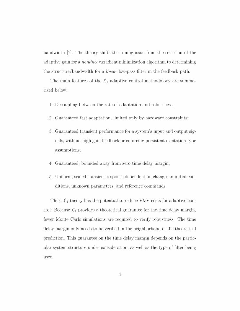
The baseline controller developed by Boeing for the X-48B aircraft con-

sists of a three axis angle of attack (AOA or α), roll rate (p), and sideslip

angle (β) control augmentation system and is designed to yield consistent

nominal system performance. This baseline controller generates virtual roll,

pitch, and yaw acceleration commands (pcmd, qcmd, rcmd), which are then

“deaugmented”, yielding moment commands Lcmd, Mcmd, and Ncmd, for

which control effort is mixed to the control surfaces accordingly. The adap-

tive element uses the feedback signals and the reference commands for α, p,

and β to augment the control signals pcmd, qcmd, and rcmd generated by the

baseline controller. Figure 2.1 presents the complete inner-loop FCS using

dynamic inversion with the L1 adaptive augmentation.

8

αre

f

βre

f

pre

f

pcm

d

q cm

d

r cm

d

δ cm

d

X-4

8BA

/CD

eaugm

enta

tion

&A

lloca

tion

Bas

elin

e

L1

CA

S

Sen

sors

y

ym

Fig

ure

2.1:

Ove

rall

Str

uct

ure

wit

hL

1A

dap

tive

Con

trol

9

2.2 Problem Formulation

A theoretical extension of the L1 adaptive control theory that compensates

for both matched as well as unmatched dynamic uncertainties was imple-

mented on the X-48B model. If uncertainty is unmatched, that simply means

that the uncertainty lies outside the span of a particular linear system’s ‘B’

matrix. For inner-loop FCS design, the effects of slow outer-loop variables

(e.g. airspeed, pitch angle, bank angle) may appear as unmatched uncer-

tainties in the dynamics of the fast inner-loop variables we are trying to

regulate (e.g. angle of attack, sideslip angle, roll rate). Also, unmodeled

nonlinearities, cross-coupling between channels, and dynamic asymmetries

may introduce unmatched uncertainties in the inner-loop system dynamics.

If the design of the inner-loop FCS does not account for these uncertainties,

their effect on the inner-loop dynamics will require continuous compensation

by the pilot, thereby increasing the pilot’s workload. Therefore, automatic

compensation for the undesirable effects of these unmatched uncertainties

on the output of the system is critical to achieve desired performance and

improve the aircraft’s handling qualities.

Next we present the theoretical framework for the development of the

L1 adaptive augmentation system that compensates for the effects of un-

matched uncertainties on the output of the system. The inner-loop dynamics

10

of the X-48B with the baseline controller can be written as:

x(t) = Amx(t) + B1 (Kgr(t) + uad(t) + f1(x(t), z(t), t))

+ B2f2(x(t), z(t), t) , x(0) = x0 ,

z(t) = go (xz(t), t) ,

xz(t) = g (xz(t), x(t), t) , xz(0) = xz0 ,

y(t) = Cx(t) ,

(2.1)

where x(t) ∈ Rn is the system state vector (measured); uad(t) ∈ R

m is

the adaptive control signal; y(t) ∈ Rm is the regulated output; Am is a

known Hurwitz n×n matrix that defines the desired dynamics for the closed-

loop system; B1 ∈ Rn×m is a known constant matrix; B2 ∈ R

n×(n−m) is a

constant matrix such that B⊤1 B2 = 0 and rank([B1 B2]) = n; C ∈ R

m×n

is a known constant matrix; Kg ∈ Rm×m is the baseline feedforward gain

matrix; r(t) ∈ Rm is the reference signal; z(t) and xz(t) are the output

and the state vector of internal unmodeled dynamics; f1(·), f2(·), go(·), and

g(·) are unknown nonlinear functions. In this problem formulation, f1(·)

represents the matched component of the uncertainties, whereas the term

B2f2(·) represents the unmatched component.

The above defined system needs to verify the following assumptions:

Assumption 1 [Stability of internal dynamics] The z-dynamics are bounded-

input-bounded-output (BIBO) stable, i.e. there exist Lz1 > 0 and Lz2 > 0

11

such that

‖zt‖L∞

= Lz1 ‖xt‖L∞

+ Lz2 .

Further, let X(t) ,

[

x⊤(t) z⊤(t)

]⊤

.

Assumption 2 [Semiglobal Lipschitz condition] For any δ > 0, there exist

positive Kδ and B such that

|fj(X1, t) − fj(X2, t)| ≤ Kδ ‖X1(t) − X2(t)‖∞ ,

|fj(0, t)| ≤ B , j = 1, 2

for all ‖Xi(t)‖∞ ≤ δ, i = 1, 2, uniformly in t.

Assumption 3 [Semiglobal uniform boundedness of partial derivatives] For

any δ > 0, there exist dfx(δ) > 0, and dft

(δ) > 0 such that for any ‖x(t)‖∞ ≤

δ, the partial derivatives of fj(X, t), j = 1, 2, are piecewise continuous and

bounded

∥∥∥∥

∂fj(X, t)

∂X

∥∥∥∥

≤ dfx(δ) ,

∣∣∣∣

∂fj(X, t)

∂t

∣∣∣∣

≤ dft(δ) , j = 1, 2 .

Assumption 4 [Stability of matched zero dynamics] The transmission zeros

of the transfer matrix from the control input u(t) to the output of the system

y(t), H1(s) = C (sI − Am)−1 B1, lie on the open left-half plane.

12

With the above formulation, the desired dynamics for the closed-loop

system are given by:

xm(t) = Amxm(t) + B1Kgr(t) , x(0) = x0 ,

ym(t) = Cx(t) .

(2.2)

In particular, if the baseline feedforward gain Kg is chosen to be Kg =

− (CA−1m B1)

−1, then the diagonal elements of the transfer matrix M(s) =

C (sI − Am)−1 B1Kg have DC gain equal to one, while the off-diagonal ele-

ments have zero DC gain.

The control objective is to design an adaptive state feedback control law

uad(t) to compensate for the effect of both the matched and unmatched

uncertainties on the output of the system y(t), and ensure that y(t) tracks

the output response of the desired system ym(t) to a given bounded reference

signal r(t) both in transient and steady-state, while all other signals remain

bounded.

2.3 L1 Adaptive Controller Formulation

Similar to previous L1 adaptive controllers, the philosophy of the L1 adaptive

state feedback controller for unmatched uncertainties is to obtain an estimate

of the uncertainties and define a control signal which compensates for the

effect of these uncertainties on the output y(t) within the bandwidth of low-

pass filters introduced in the feedback loop. These filters guarantee that the

13

L1 adaptive controller stays in the low-frequency range even in the presence

of fast adaptation and large reference inputs. The choice of the low-pass

filters leads to separation between performance and robustness. Adaptation

is based on a piecewise constant adaptive law and uses the output of a state

predictor to update the estimate of the uncertainties.

The elements of L1 adaptive controller are introduced below.

State Predictor:

˙x(t) = Amx(t) + B1Kgr(t) + B1 (uad(t) + σ1(t)) + B2σ2(t)

x(0) = x0

y(t) = Cx(t)

(2.3)

The state predictor replicates the closed-loop system structure, with the es-

timates σ1(t) and σ2(t) replacing the unknown parameters and using the

adaptive control signal uad(t) defined below.

Adaptive Laws:

The adaptive parameters are governed by the following piecewise constant

adaptive law:

σ1(t) = σ1(kTs) , σ2(t) = σ2(kTs) , t ∈ [kTs, (k + 1)Ts]

14

σ1(kTs)

σ2(kTs)

= −

[

B1 B2

]−1

Φ−1(Ts)eAmTs x(kTs) (2.4)

k = 0, 1, 2, ...

where Ts is the sampling rate of the model, Φ(Ts) = A−1m

(eAmTs − I

), and

x(t) = x(t) − x(t) is updated every Ts.

Control Law:

uad(s) = −C1(s)σ1(s)︸ ︷︷ ︸

uad1

− C2(s)H−11 (s)H2(s)σ2(s)

︸ ︷︷ ︸

uad2

(2.5)

where

H1(s) = Cm (sI − Am)−1 B1 , H2(s) = Cm (sI − Am)−1 B2 .

C1(s) is a strictly proper stable filter and C2(s) is selected to ensure that

C2(s)H−11 (s)H2(s) is also proper and stable. Furthermore, the transmission

zeros of H1(s) need to lie on the open left-half plane. Regarding the struc-

ture of uad2, note that H2(s)σ2(s) is the estimated effect of the unmatched

uncertainties on the output of the plant, while −H−11 (s)H2(s)σ2(s) would be

the control signal needed to cancel this effect. The low-pass filters C1(s)

and C2(s) serve to attenuate high frequencies in the adaptive control signals,

15

and thus define the performance-robustness trade-off. By designing a filter

with a lower cutoff frequency, the robustness of the adaptive controller can

be systematically tuned to increase the time delay margin. Similarly a filter

with a higher cutoff frequency will exhibit improved performance, at the cost

of a reduced time delay margin. The proof of the performance bounds of this

architecture can be found in Ref. [19]

Although the L1 adaptive controller does not require gain scheduling, it

can be used to augment a gain scheduled baseline controller, as is the case

for the X-48B. Thus, one can specify varying desired performance specifica-

tions across the flight envelope without changing the adaptive portion of the

controller. Also, the rate of adaptation is decoupled from the robustness of

the controller. and limited only by hardware (or simulation step time) con-

straints. The trade-off between performance and robustness is determined

by the low-pass filters on the adaptive control signals, not by an adaptive

gain. By decreasing the bandwidth of this filter, robustness can be improved

with reduced performance, and vice versa.

The reader will find in Ref. [17] an application of this same extension of

the L1 adaptive control theory to the design of an inner-loop FCS for the

NASA Airborne Subscale Transport Aircraft Research (AirSTAR) system.

The main difference between these two designs is that, while in this paper

we use the L1 adaptive controller as an augmentation system, we consider a

full adaptive FCS without a baseline controller for the the AirSTAR.

16

Chapter 3

Simulation Results

3.1 Remarks on the Implementation

High-fidelity, six degree of freedom linear Simulink models of the X-48B

were provided by Boeing for a wide range of flight conditions, up to post

stall angle of attack and maximum sideslip. The L1 adaptive controller was

then implemented in Simulink to augment the baseline longitudinal, lateral,

and directional control laws. The simulation contained the baseline X-48B

inner-loop control laws, sensor processing and filtering, as well as actuator

dynamics. The baseline control laws of the X-48B model were not modified,

and the entire controller (including the L1 adaptive controller) was simulated

at the original sampling rate of 200 Hz. Here L1 adaptive controller was

designed strictly for pilot-in-the-loop flying, hence there is no outer-loop

compensation to hold altitude, speed, or bank angle. A single-input single-

17

output L1 adaptive controller was added to each of the three control channels

(Figure 3.1). The adaptive control architecture for each channel was exactly

the same, consisting of the control law, state predictor, and adaptive law.

These are the three basic components required for any implementation of an

L1 adaptive control system.

Using this SISO structure, the L1 controller in the longitudinal channel

augmented the pitch acceleration command generated by the baseline con-

troller to achieve the desired longitudinal dynamics specified by the state

predictor. Likewise, the lateral and directional channels independently aug-

mented the baseline roll and yaw acceleration commands, respectively. The

state predictor for each channel was constructed to mimic a transfer function

specifying that channel’s desired dynamics. These desired dynamics were

second-order for the longitudinal and directional channels and first-order for

the roll response.

At each flight condition, the state predictor matrices Am, B1, and B2

were recomputed using the provided state space models of the control input

deaugmentation, allocation, and aircraft response (Figure 2.1). A vector of

state feedback gains was used with the system matrix B1 to place the state

predictor poles at the locations specified by the desired dynamics transfer

functions. Am is the matrix resulting from this pole placement. The matrix

B2 is straightforwardly computed to satisfy the conditions B⊤

1 B2 = 0 and

rank([B1 B2]) = n as specified in Section 2.2. Thus the state predictor ma-

trices Am and B1 ultimately represent the desired, decoupled dynamics with

18

either pdes, qdes, or rdes as the input, depending on the channel, while B2 ulti-

mately allows the adaptive controller to compensate for uncertainty outside

the span of B1. It is important to note that the input to the state predictor

must always be the same as the control input that is being augmented, in

this case the acceleration commands.

Finally, the low-pass filters C1(s) and C2(s), for the matched and un-

matched uncertainty channels respectively, are chosen as first-order filters

and their bandwidth is adjusted based on the desired trade-off between per-

formance and robustness.

19

Lon

gitu

din

al

Dir

ection

al

Lat

eral

L1

CA

S

q cm

d

pcm

d

r cm

d

αre

f

pre

f

βre

f p

[α q

]

[β r

]

(a)L

1C

AS

Arc

hitec

ture

L1

Adap

tive

Con

trol

ler

Con

trol

Law

Law

Adap

tive

Sta

teP

redic

tor

uad

uad1

uad2

x

x

yre

f

x

−

[σ

m σ2

]

(b)L

1C

ontr

oller

Str

uct

ure

Fig

ure

3.1:

L1

Adap

tive

Con

trol

Augm

enta

tion

Syst

em

20

3.2 Results at Stall AOA Trim

Adding the L1 adaptive controller greatly improved angle of attack, sideslip,

and roll rate command tracking, particularly at high angles of attack. The

following plots represent deviations from the trim conditions. Small reference

commands were used because the models were derived from linearizations at

a particular flight condition. Figure 3.2a shows the angle of attack tracking

performance for a pitch doublet at stall angle of attack trim. One can see from

Figures 3.2b and 3.2c that there is strong coupling between the longitudinal

and lateral/directional dynamics, due primarily to nonzero sideslip trim. The

pitch command leads to large changes in sideslip and roll rate. However,

with the L1 adaptive controller, the aircraft maintains sideslip and roll rate

significantly closer to trim conditions than with the baseline controller alone.

We also note that the L1 adaptive controller does not lead to high frequencies

in the control surface deflections (Figure 3.2d).

The L1 adaptive augmentation also maintains improved performance in

the event of control surface failures. Performance is recovered without the

use of failure detection and isolation methods. Figure 3.3 shows the angle

of attack tracking performance of the baseline controller versus its perfor-

mance with the L1 adaptive controller with a symmetric 80% loss of control

effectiveness in the inboard elevons, representing half of the total number of

control surfaces. The L1 adaptive controller did not require any retuning or

reconfiguration from the nominal case to compensate for this failure. When

21

0 2 4 6 8 10 12−3

−2

−1

0

1

2

3

time [s]

∆α [d

eg]

∆αcmd

∆α − baseline∆α − L1 + baseline

(a) Angle of Attack

0 2 4 6 8 10 12−6

−4

−2

0

2

4

6

time [s]

∆β [d

eg]

∆βcmd

∆β − baseline∆β − L1 + baseline

(b) Sideslip

0 2 4 6 8 10 12−20

−15

−10

−5

0

5

10

15

20

time [s]

∆ p

[dps

]

∆ p

cmd

∆ p − baseline∆ p − L1 + baseline

(c) Roll Rate

0 2 4 6 8 10 12−40

−20

0

20

40

time [s]

defle

ctio

n [d

eg]

0 2 4 6 8 10 12−40

−20

0

20

40

time [s]

defle

ctio

n [d

eg]

(d) Control Surface Deflections with BaselineController (Top) and with L1 CAS (Bottom)

Figure 3.2: Pitch Command at Stall AOA Trim

22

0 2 4 6 8 10 12−6

−4

−2

0

2

4

6

8

10

time [s]

∆α [d

eg]

∆α

cmd

∆α − baseline − w/failure∆α − L1 + baseline − w/failure

Figure 3.3: AOA Tracking at Stall AOA Trim, with Failure

the failure is introduced, the tracking performance with L1 augmentation

exhibits a slower transient response with increased oscillation, but the air-

craft generally tracks the reference command. Without L1 augmentation,

the baseline controller is incapable of tracking the reference command and

the system becomes unstable.

3.3 Results at Normal Flight AOA Trim

The same design, without any retuning, was applied for flight conditions at

low angles of attack. Specifically, “without any retuning” means that the

sampling time of the adaptive laws and the design of the filter remained the

same. The benefits of L1 adaptive augmentation are shown here for a normal

23

flight angle of attack trim condition. Again, small reference commands were

used because the given models are linearized about a single flight condition.

With a symmetric 80% loss of control effectiveness in the inboard elevons

the L1 augmented baseline controller enables the aircraft to nearly recover

the nominal performance (Figure 3.4a). Figures 3.4b and 3.4c show that the

L1 augmentation does not lead to undesirable behavior in the directional

and lateral dynamics. The L1 augmentation also eliminates the steady state

error in the roll rate tracking, in the absence any control surface failures (Fig-

ure 3.5c). Figures 3.5a and 3.5b again show that the L1 augmentation does

not produce undesirable behavior in the longitudinal or directional dynam-

ics. Note that the αcmd in Figure 3.5a is not commanded directly. Rather, it

arises in response to additional logic based on the aircraft’s response to the

roll rate command.

In addition to the 80% loss of control effectiveness, the case of 200% con-

trol effectiveness, corresponding to increasing the loop gain by a factor of two,

was checked to ensure at least a 6 dB gain margin. As Figure 3.9 shows, the

L1 adaptive controller remains stable given this increase in control effective-

ness, and in fact reduces the amount of overshoot exhibited by the baseline

controller alone. Again, the controller was in no way retuned or redesigned

to compensate for this failure, which highlights the fact that the L1 control

augmentation system does not require changes to the filter design or rate of

adaptation for unpredictable changes in a system’s dynamics.

24

0 2 4 6 8 10 12−1.5

−1

−0.5

0

0.5

1

1.5

2

2.5

3

3.5

time [s]

∆α (

deg)

∆α

cmd

∆α − baseline∆α − L1 + baseline∆α − baseline − w/failure∆α − L1 + baseline − w/failure

(a) Angle of Attack

0 2 4 6 8 10 12−1

−0.5

0

0.5

1

1.5

2

time [s]

∆β (

deg)

∆β

cmd

∆β − baseline∆β − L1 + baseline∆β − baseline − w/failure∆β − L1 + baseline − w/failure

(b) Sideslip

0 2 4 6 8 10 12−2

−1

0

1

2

3

4

5

time [s]

∆ p

(dps

)

∆ p

cmd

∆ p − baseline∆ p − L1 + baseline∆ p − baseline − w/failure∆ p − L1 + baseline − w/failure

(c) Roll Rate

Figure 3.4: Pitch Command at Normal Flight AOA Trim

25

0 2 4 6 8 10 12−1

−0.5

0

0.5

1

1.5

2

2.5

3

time [s]

∆α (

deg)

∆α

cmd

∆α − baseline

∆α − L1 + baseline

(a) Angle of Attack

0 2 4 6 8 10 12−1

−0.5

0

0.5

1

1.5

2

time [s]

∆β (

deg)

∆β

cmd

∆β − baseline∆β − L1 + baseline

(b) Sideslip

0 2 4 6 8 10 12−25

−20

−15

−10

−5

0

5

10

15

20

25

time [s]

∆ p

(dps

)

∆ p − baseline

∆ pcmd

∆ p − L1 + baseline

(c) Roll Rate

Figure 3.5: Roll Rate Command at Normal Flight AOA Trim

26

0 2 4 6 8 10 12−2

−1.5

−1

−0.5

0

0.5

1

1.5

2

time [s]

∆α (

deg)

∆α

cmd

∆α − baseline

∆α − L1 + baseline

Figure 3.6: AOA Tracking with 200% Control Effectiveness

27

3.4 Time Delay Margin

For the above examples, the adaptive control signal passes through a first

order filter. By reducing the bandwidth of the filter, and thus attenuating

more of the adaptive control signal, the time delay margin of the system can

be systematically increased at the cost of reduced performance. Likewise,

by increasing the bandwidth of the filter the performance of adaptive closed-

loop system can be arbitrarily improved, at the cost of reduced robustness.

Table 3.1 summarizes the time delay margins for simulations at the two angle

of attack trim conditions previously described, using various bandwidths (ω)

for a first-order filter on the adaptive control signal. We determined these

margins by seeing how much time delay the system could tolerate at its input

before becoming marginally stable. The time delay margins were checked

both with and without an asymmetric loss of control effectiveness, which

affected all three control channels. The margins given below are in addition

to any time delay that is already modeled in the X-48B simulation. These

results are slightly improved from those in [1] due to the addition of actuator

dynamics in the state predictor.

To demonstrate this performance/robustness trade-off, the time delay

margin was increased from 50 ms to 135 ms for the “no failure” condition at

normal flight angle of attack trim, at the expense of some performance. To

achieve these improved time delay margins, a first order filter with a band-

width of 4 rad/s was used, compared with 15 rad/s in Figures 3.4 and 3.5.

28

By comparing Figures 3.7 and 3.8 with Figures 3.4a and 3.5c, one can ob-

serve the trade-off in performance to achieve improved time delay margin for

this example. Likewise, the time delay margin for the “no failure” condition

at stall angle of attack trim was increased from 30 ms to 100 ms. For this

case the trade-off between performance and robustness can be seen by com-

paring Figure 3.9 with Figure 3.2a. Figure 3.10 shows that we are still able

to compensate for failures at stall angles of attack, even with the reduced

bandwidth filter. This figure can be compared with Figure 3.3.

Thus, the performance-robustness trade-off for the L1 adaptive controller

can be reduced to the selection of the bandwidth of a first-order filter.

LMI techniques can also be utilized to determine an optimal filter struc-

ture (not necessarily first-order) that maximizes the time delay margin for

the given desired performance level [20]. Further detailed analysis of the per-

formance/robustness trade-off in terms of filter optimization is not pursued

in this thesis.

29

AO

ATrim

Failure

Base

line

margin

L1

+B

ase

line

margin

ω=

15ω

=8

ω=

4N

orm

alN

one

250m

s50

ms

85m

s13

5ms

Nor

mal

Asy

m.

80%

LO

C35

0ms

70m

s10

5ms

155m

sSta

llN

one

160m

s30

ms

50m

s10

0ms

Sta

llA

sym

.80

%LO

CN

oper

form

ance

55m

s80

ms

125m

s

Tab

le3.

1:T

ime

Del

ayM

argi

nC

ompar

ison

30

0 2 4 6 8 10 12−1.5

−1

−0.5

0

0.5

1

1.5

2

2.5

3

3.5

time [s]

∆α (

deg)

∆α

cmd

∆α − baseline∆α − L1 + baseline∆α − baseline − w/failure∆α − L1 + baseline − w/failure

Figure 3.7: AOA Tracking with Reduced Bandwidth Filter at Normal FlightAOA Trim

0 2 4 6 8 10 12−25

−20

−15

−10

−5

0

5

10

15

20

25

time [s]

∆ p

(dps

)

∆ p

cmd

∆ p − baseline

∆ p − L1 + baseline

Figure 3.8: Roll Rate Tracking with Reduced Bandwidth Filter at NormalFlight AOA Trim

31

0 2 4 6 8 10 12−3

−2

−1

0

1

2

3

time [s]

∆α (

deg)

∆α

cmd

∆α − baseline

∆α − L1 + baseline

Figure 3.9: AOA Tracking with Reduced Bandwidth Filter at Stall AOATrim

0 2 4 6 8 10 12−6

−4

−2

0

2

4

6

8

10

time [s]

∆α (

deg)

∆α

cmd

∆α − baseline∆α − L1 + baseline

Figure 3.10: AOA Tracking with Reduced Bandwidth Filter at Stall AOATrim with Failure

32

3.5 Comparison of Virtual Control Commands

Finally, we verified that the low-pass filters in the control law ensure that

the virtual roll, pitch, and yaw commands are in the low frequency range.

The filters can be straightforwardly designed to achieve comparable adap-

tive control signal amplitudes and rates with respect to Boeing’s baseline

controller. Figure 3.11 compares the system response with the baseline con-

troller and the L1 adaptive augmentation using a 4 rad/s) filter bandwidth,

which achieves a 135 ms time delay margin. The virtual commands given by

baseline controller and the L1 augmented controller are compared in Figure

3.12, along with their derivatives. It can be seen that the derivatives of the

control signals with L1 and the baseline are very similar. It is important that

the derivatives of the control action do not contain high frequencies, which

may excite structural modes of an aircraft.

33

0 2 4 6 8 10 12−2

−1.5

−1

−0.5

0

0.5

1

1.5

2

time [s]

∆α (

deg)

∆α

cmd

∆α − baseline

∆α − L1 + baseline

(a) AOA Tracking at Normal Flight AOATrim

0 2 4 6 8 10 12−0.5

0

0.5

1

1.5

time [s]

∆β (

deg)

∆β

cmd

∆β − baseline∆β − L1 + baseline

(b) Sideslip Maintenance at Normal FlightAOA Trim

0 2 4 6 8 10 12−1

−0.5

0

0.5

1

1.5

2

time [s]

∆ p

(dps

)

∆ p

cmd

∆ p − baseline∆ p − L1 + baseline

(c) Roll Rate Maintenance at Normal FlightAOA Trim

Figure 3.11: Pitch Command at Normal Flight AOA Trim with ReducedBandwidth Filter

34

0 2 4 6 8 10 12−100

−50

0

50

100

time [s]

long

itudi

nal c

omm

and

[dps

2 ]

0 2 4 6 8 10 12−2

−1

0

1

2x 10

4

time [s]

long

itudi

nal c

md

rate

[dps

3 ]

0 2 4 6 8 10 12−10

−5

0

5

10

time [s]

late

ral c

omm

and

[dps

2 ]

0 2 4 6 8 10 12−100

−50

0

50

100

time [s]

late

ral c

md

rate

[dps

3 ]

0 2 4 6 8 10 12

−2

0

2

time [s]

dire

ctio

nal c

omm

and

[dps

2 ]

0 2 4 6 8 10 12−10

−5

0

5

10

time [s]dire

ctio

nal c

md

rate

[dps

3 ]

(a) Baseline Controller Commands and Derivatives

0 2 4 6 8 10 12−100

−50

0

50

100

time [s]

long

itudi

nal c

omm

and

[dps

2 ]

0 2 4 6 8 10 12−2

−1

0

1

2x 10

4

time [s]

long

itudi

nal c

md

rate

[dps

3 ]

0 2 4 6 8 10 12−10

−5

0

5

10

time [s]

late

ral c

omm

and

[dps

2 ]

0 2 4 6 8 10 12−100

−50

0

50

100

time [s]

late

ral c

md

rate

[dps

3 ]

0 2 4 6 8 10 12

−2

0

2

time [s]

dire

ctio

nal c

omm

and

[dps

2 ]

0 2 4 6 8 10 12−10

−5

0

5

10

time [s]

dire

ctio

nal c

md

rate

[dps

3 ]

(b) L1 CAS Commands and Derivatives

Figure 3.12: Comparison of Virtual Pitch, Roll, and Yaw Acceleration Com-mands and Their Derivatives

35

Chapter 4

Conclusions and Future Work

An L1 adaptive control augmentation system that compensates for both

matched and unmatched uncertainty has been presented for the X-48B Blended

Wing Body. The L1 adaptive control theory was validated on a wide range of

linear models of the X-48B in the presence of various failures. In these sim-

ulations, L1 adaptive augmentation demonstrates the potential for greatly

improved performance for nominal flight conditions across the entire enve-

lope with guaranteed robustness. In the event of a failure, the L1 adaptive

controller adapts to recover desired aircraft performance and provide a pre-

dictable response to pilot inputs.

L1 theory has been extended to support input saturation constraints,

such as control surface deflection limits. Control surface deflection and rate

limits were not part of the X-48B models provided for this challenge problem.

If higher fidelity models of the aircraft’s dynamics could also be obtained,

36

the performance benefits of and L1 control augmentation system could be

demonstrated in further detail. Future work could also include determining

an appropriate minimum time delay margin for the X-48B models, tuning

the filter to achieve this time delay margin, and analyzing the performance-

robustness trade-off according to a true design requirement.

37

References

[1] Tyler Leman, Enric Xargay, Geir Dullerud, Naira Hovakimyan, and

Thomas Wendel. L1 Adaptive Control Augmentation System for the

X-48B Aircraft. In AIAA Guidance, Navigation, and Control Confer-

ence, Chicago, IL, August 2009.

[2] Jaiwon Shin. The NASA Aviation Safety Program: Overview. March

2000. NASA/TM2000-209810.

[3] Zhuquan Zang and Robert R. Bitmead. Transient Bounds for Adaptive

Control Systems. In 30th IEEE Conference on Decision and Control,

pages 2724–2729, Brighton, U.K., December 1990.

[4] Chengyu Cao and Naira Hovakimyan. Design and Analysis of a Novel L1

Adaptive Control Architecture with Guaranteed Transient Performance.

IEEE Transactions on Automatic Control, 53(3):586–591, 2008.

[5] Chengyu Cao and Naira Hovakimyan. Guaranteed Transient Perfor-

mance with L1 Adaptive Controller for Systems with Unknown Time-

Varying Parameters and Bounded Disturbances: Part I. In Proc. of

38

American Control Conference, pages 3925–3930, New York, NY, July

2007.

[6] Chengyu Cao and Naira Hovakimyan. Stability Margins of L1 Adaptive

Controller: Part II. In Proc. of American Control Conference, pages

3931–3936, New York, NY, July 2007.

[7] Chengyu Cao and Naira Hovakimyan. L1 Adaptive Controller for a Class

of Systems with Unknown Nonlinearities: Part I. In Proc. of American

Control Conference, pages 4093–4098, Seattle, WA, June 2008.

[8] Isaac Kaminer, Oleg Yakimenko, Vladimir Dobrokhodov, Antonio Pas-

coal, Naira Hovakimyan, Chengyu Cao, Amanda Young, and Vijay V.

Patel. Coordinated Path Following for Time-Critical Missions of Mul-

tiple UAVs via L1 Adaptive Output Feedback Controllers. In AIAA

Guidance, Navigation, and Control Conference, Hilton Head Island, SC,

August 2007.

[9] Chengyu Cao, Naira Hovakimyan, Isaac Kaminer, Vijay V. Patel, and

Vladimir Dobrokhodov. Stabilization of Cascaded Systems via L1 Adap-

tive Controller with Application to a UAV Path Following Problem and

Flight Test Results. In American Control Conference, New York, NY,

July 2007.

[10] Randy W. Beard, Nathan B. Knoebel, Chengyu Cao, Naira Hov-

akimyan, and Joshua S. Matthews. An L1 Adaptive Pitch Controller

39

for Miniature Air Vehicles. In AIAA Guidance, Navigation, and Control

Conference, Keystone, CO, August 2006.

[11] Jiang Wang, Vijay V. Patel, Chengyu Cao, Naira Hovakimyan, and

Eugene Lavretsky. L1 Adaptive Controller for Tailless Unstable Aircraft

in the presence of Unknown Actuator Failures. In AIAA Guidance,

Navigation, and Control Conference, Hilton Head Island, SC, August

2007.

[12] Jiang Wang, Chengyu Cao, Vijay V. Patel, Naira Hovakimyan, and

Eugene Lavretsky. L1 Adaptive Neural Network Controller for Au-

tonomous Aerial Refueling with Guaranteed Transient Performance. In

AIAA Guidance, Navigation, and Control Conference, Keystone, CO,

August 2006.

[13] Jiang Wang, Vijay V. Patel, Chengyu Cao, Naira Hovakimyan, and

Eugene Lavretsky. L1 Adaptive Neural Network Controller for Au-

tonomous Aerial Refueling with Guaranteed Transient Performance. In

AIAA Guidance, Navigation, and Control Conference, Keystone, CO,

August 2006.

[14] Irene M. Gregory, Chengyu Cao, Vijay V. Patel, and Naira Hovakimyan.

L1 Adaptive Control Laws for Flexible Semi-Span Wind Tunnel Model

of High-Aspect Ratio Flying Wing. In AIAA Guidance, Navigation, and

Control Conference, Hilton Head Island, SC, August 2007.

40

[15] Chengyu Cao, Naira Hovakimyan, and Eugene Lavretsky. Application of

L1 Adaptive Controller to Wing Rock. In AIAA Guidance, Navigation,

and Control Conference, Keystone, CO, August 2006.

[16] Yu Lei, Chengyu Cao, Eugene Cliff, Naira Hovakimyan, Andy Kurdila,

Michael Bolender, and David Doman. Design of an L1 Adaptive Con-

troller for an Air-Breathing Hypersonic Vehicle Model with Unmodelled

Dynamics. In AIAA Guidance, Navigation, and Control Conference,

Hilton Head Island, SC, August 2007.

[17] Irene M. Gregory, Chengyu Cao, Enric Xargay, Naira Hovakimyan, and

Xiaotian Zou. L1 Adaptive Control Design for NASA AirSTAR Flight

Test Vehicle. In AIAA Guidance, Navigation, and Control Conference,

Chicago, IL, August 2009.

[18] NASA Dryden Flight Research Center. X-48B Blended

Wing Body. Retrieved January 15, 2009 from

http://www.nasa.gov/centers/dryden/research/X-48B/index.html.

[19] Enric Xargay, Chengyu Cao, and Naira Hovakimyan. L1 Adaptive Con-

troller for Nonlinear Multi-Input Multi-Output Systems in the Presence

of Significant Cross-Coupling. In American Control Conference, Balti-

more, MD, June 2010.

[20] Dapeng Li, Naira Hovakimyan, Chengyu Cao, and Kevin A. Wise. Filter

Design for Feedback-loop Trade-off of L1 Adaptive Controller: A Lin-

41

ear Matrix Inequality Approach. In AIAA Guidance, Navigation, and

Control Conference, Honolulu, HI, August 2008.

42