kva and mva: capital valuation adjustment and margin ... · pdf filekva and mva: capital...

KVA and MVA: Capital Valuation Adjustmentand Margin Valuation Adjustment

Andrew Green

Head of CVA/FVA Quantitative Research

Lloyds Bank

July 2015

2

The views expressed in the following material are the

author’s and do not necessarily represent the views of

the Global Association of Risk Professionals (GARP),

its Membership or its Management.

Contents

1 Introducing KVA and MVA

2 Pricing Capital and Initial Margin by Replication

3 KVA Examples

4 Calculating MVA

5 MVA: Numerical ExamplesClearing: XVA vs MVA

6 KVA, MVA and Accounting

7 Conclusions

8 Bibliography

KVA & MVA

Disclaimer

Joint work with Chris Kenyon and Chris Dennis The views expressed in

this presentation are the personal views of the speaker and do notnecessarily reflect the views or policies of current or previous employers.

Chatham House Rules apply to the reporting on this presentation and thecomments of the speaker.

A. Green 01.07.2015 3 / 62

KVA & MVA

Introducing KVA and MVA

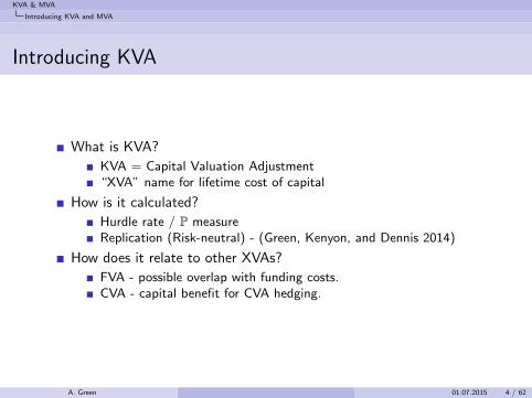
Introducing KVA

What is KVA?

KVA = Capital Valuation Adjustment“XVA” name for lifetime cost of capital

How is it calculated?

Hurdle rate / P measureReplication (Risk-neutral) - (Green, Kenyon, and Dennis 2014)

How does it relate to other XVAs?

FVA - possible overlap with funding costs.CVA - capital benefit for CVA hedging.

A. Green 01.07.2015 4 / 62

KVA & MVA


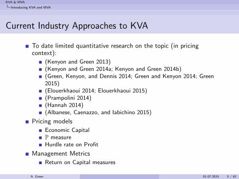
Current Industry Approaches to KVA

To date limited quantitative research on the topic (in pricingcontext):

(Kenyon and Green 2013)(Kenyon and Green 2014a; Kenyon and Green 2014b)(Green, Kenyon, and Dennis 2014; Green and Kenyon 2014; Green2015)(Elouerkhaoui 2014; Elouerkhaoui 2015)(Prampolini 2014)(Hannah 2014)(Albanese, Caenazzo, and Iabichino 2015)

Pricing models

Economic CapitalP measureHurdle rate on Profit

Management Metrics

Return on Capital measures

A. Green 01.07.2015 5 / 62

KVA & MVA


Introducing MVA

What is MVA?

MVA = (Initial) Margin Valuation Adjustment“XVA” name for funding cost of initial marginApplies to CCP Margin and Bilateral Margin (BCBS-317 2015;BCBS-261 2013; BCBS-242 2013; BCBS-226 2012)

How is it calculated?

Replication modelIntegral over expected initial margin profile.

How does it relate to other XVAs?

No overlap.There are trade-offs vs other XVAs.

A. Green 01.07.2015 6 / 62

KVA & MVA


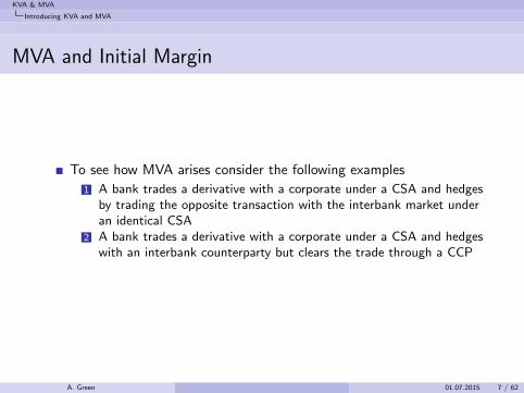
MVA and Initial Margin

To see how MVA arises consider the following examples

1 A bank trades a derivative with a corporate under a CSA and hedgesby trading the opposite transaction with the interbank market underan identical CSA

2 A bank trades a derivative with a corporate under a CSA and hedgeswith an interbank counterparty but clears the trade through a CCP

A. Green 01.07.2015 7 / 62

KVA & MVA


Case 1: Back-to-Back Trade CSA

Bank Corporate Market Interest Rate Swap A Interest Rate Swap B

Case I Trade A –ve Value

to Corp

Trade A +ve Value to Bank

Trade B -ve Value

to Bank

Trade B +ve Value

to Mkt

Corporate Gives Collateral to Bank

Bank Rehypothecates Collateral to Market

Variation Margin

Case II Trade A

+ve Value to Corp

Trade A -ve Value to Bank

Trade B +ve Value

to Bank

Trade B -ve Value

to Mkt

Bank Rehypothecates Collateral to Corporate

Market gives Collateral to Bank

Variation Margin

A. Green 01.07.2015 8 / 62

KVA & MVA


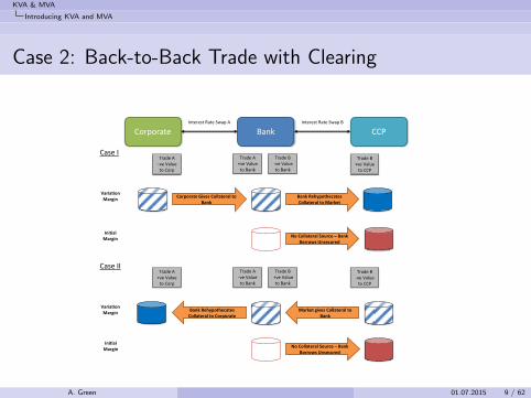
Case 2: Back-to-Back Trade with Clearing

Bank Corporate CCP Interest Rate Swap A Interest Rate Swap B

Case I Trade A –ve Value

to Corp

Trade A +ve Value to Bank

Trade B -ve Value

to Bank

Trade B +ve Value

to CCP

Corporate Gives Collateral to Bank

Bank Rehypothecates Collateral to Market

Variation Margin

Case II Trade A

+ve Value to Corp

Trade A -ve Value to Bank

Trade B +ve Value

to Bank

Trade B -ve Value

to CCP

Bank Rehypothecates Collateral to Corporate

Market gives Collateral to Bank

Variation Margin

No Collateral Source – Bank Borrows Unsecured

Initial Margin

No Collateral Source – Bank Borrows Unsecured

Initial Margin

A. Green 01.07.2015 9 / 62

KVA & MVA


Funding cost of Margin = MVA

Intuitively initial margin must be funded as in most casesrehypothecation of the initial margin is not allowed.

Leads to a new valuation adjustment: Margin Valuation Adjustment

Valuation of derivatives under collateralisation (VM) is now wellestablished - (Piterbarg 2010; Piterbarg 2012; Piterbarg 2013)

How do we model the funding cost of margin?

A. Green 01.07.2015 10 / 62

KVA & MVA

Pricing Capital and Initial Margin by Replication

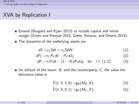
XVA by Replication I

Extend (Burgard and Kjaer 2013) to include capital and initialmargin (Green and Kenyon 2015; Green, Kenyon, and Dennis 2014).

The dynamics of the underlying assets are

dS =µsSdt + σsSdW (1)

dPC =rCPCdt − PCdJC (2)

dPi =riPidt − (1− Ri )PidJB for i ∈ {1, 2} (3)

On default of the issuer, B, and the counterparty, C , the value thederivative takes is

V (t,S , 1, 0) =gB(MB ,X ) (4)

V (t,S , 0, 1) =gC (MC ,X ). (5)

A. Green 01.07.2015 11 / 62

KVA & MVA


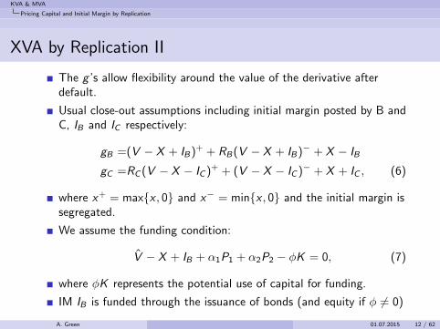
XVA by Replication II

The g ’s allow flexibility around the value of the derivative afterdefault.

Usual close-out assumptions including initial margin posted by B andC, IB and IC respectively:

gB =(V − X + IB)+ + RB(V − X + IB)− + X − IB

gC =RC (V − X − IC )+ + (V − X − IC )− + X + IC , (6)

where x+ = max{x , 0} and x− = min{x , 0} and the initial margin issegregated.

We assume the funding condition:

V − X + IB + α1P1 + α2P2 − φK = 0, (7)

where φK represents the potential use of capital for funding.

IM IB is funded through the issuance of bonds (and equity if φ 6= 0)

A. Green 01.07.2015 12 / 62

KVA & MVA


XVA by Replication III

There is no IC in equation (7) as we have assumed that initialmargin cannot be rehypothecated.

The growth in the cash account positions (prior to rebalancing) are

d βS =δ(γS − qS)Sdt (8)

d βC =− αCqCPCdt (9)

d βX =− rXXdt (10)

d βK =− γK (t)Kdt (11)

d βI =rIB IBdt − rIC ICdt, (12)

where an additional cash account is now included for any return oninitial margin.

The growth in cash account associated with capital d βK representsthe payment of a dividend yield γK on the capital K borrowed fromshareholders

A. Green 01.07.2015 13 / 62

KVA & MVA


XVA by Replication IV

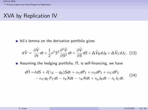
Ito’s lemma on the derivative portfolio gives

dV =∂V

∂tdt +

1

2σ2S2 ∂

2V

∂S2dt +

∂V

∂SdS + ∆VBdJB + ∆VCdJC . (13)

Assuming the hedging portfolio, Π, is self-financing, we have

dΠ =δdS + δ(γS − qS)Sdt + α1dP1 + α2dP2 + αCdPC

− αCqCPCdt − rXXdt − γKKdt + rIB IBdt − rIC ICdt.(14)

A. Green 01.07.2015 14 / 62

KVA & MVA


XVA by Replication V

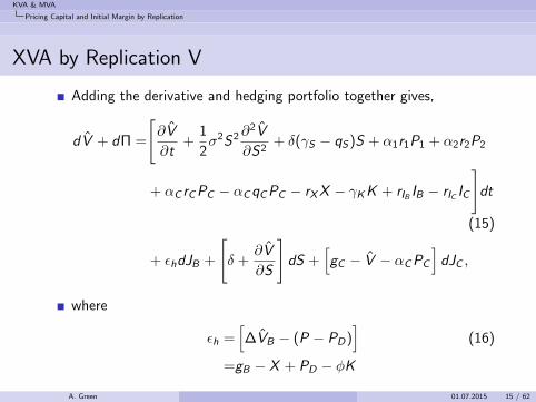
Adding the derivative and hedging portfolio together gives,

dV + dΠ =

[∂V

∂t+

1

2σ2S2 ∂

2V

∂S2+ δ(γS − qS)S + α1r1P1 + α2r2P2

+ αC rCPC − αCqCPC − rXX − γKK + rIB IB − rIC IC

]dt

(15)

+ εhdJB +

[δ +

∂V

∂S

]dS +

[gC − V − αCPC

]dJC ,

where

εh =[∆VB − (P − PD)

](16)

=gB − X + PD − φK

A. Green 01.07.2015 15 / 62

KVA & MVA


XVA by Replication VI

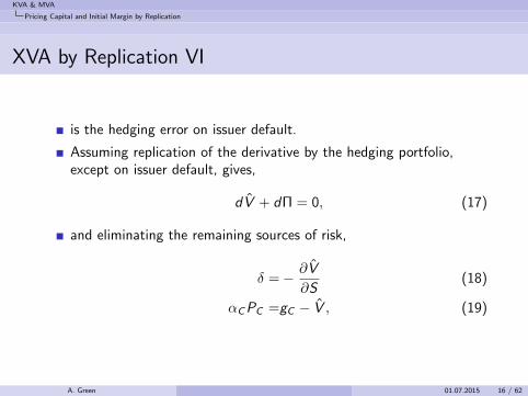
is the hedging error on issuer default.

Assuming replication of the derivative by the hedging portfolio,except on issuer default, gives,

dV + dΠ = 0, (17)

and eliminating the remaining sources of risk,

δ =− ∂V

∂S(18)

αCPC =gC − V , (19)

A. Green 01.07.2015 16 / 62

KVA & MVA


XVA by Replication VII

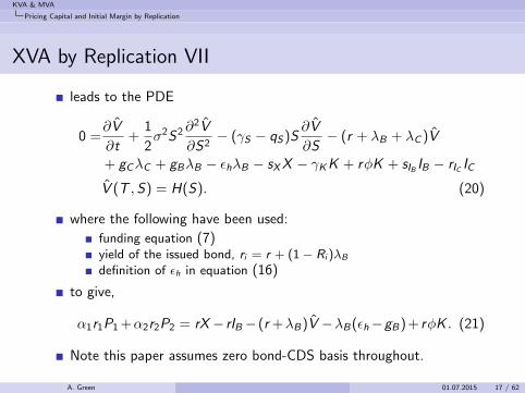
leads to the PDE

0 =∂V

∂t+

1

2σ2S2 ∂

2V

∂S2− (γS − qS)S

∂V

∂S− (r + λB + λC )V

+ gCλC + gBλB − εhλB − sXX − γKK + rφK + sIB IB − rIC IC

V (T ,S) = H(S). (20)

where the following have been used:

funding equation (7)yield of the issued bond, ri = r + (1− Ri )λB

definition of εh in equation (16)

to give,

α1r1P1 +α2r2P2 = rX − rIB− (r +λB)V −λB(εh−gB) + rφK . (21)

Note this paper assumes zero bond-CDS basis throughout.

A. Green 01.07.2015 17 / 62

KVA & MVA


XVA by Replication VIII

Writing, V , as the sumV = V + U (22)

recognising that V satisfies the Black-Scholes PDE,

∂V

∂t+

1

2σ2S2 ∂

2V


∂V

∂S− rV =0

V (T ,S) =0, (23)

gives a PDE for the valuation adjustment, U,

∂U

∂t+

1

2σ2S2 ∂

2U


∂U

∂S− (r + λB + λC )U =

VλC − gCλC + VλB − gBλB + εhλB + sXX − sIB IB + γKK − rφK

U(T ,S) = 0 (24)

A. Green 01.07.2015 18 / 62

KVA & MVA


XVA by Replication IX

Applying Feynman-Kac gives,

U = CVA + DVA + FCA + COLVA + KVA, (25)

where

CVA =−∫ T

t

λC (u)e−∫ ut

(r(s)+λB (s)+λC (s))ds

× Et [V (u)− gC (V (u),X (u))] du (26)

DVA =−∫ T

t

λB(u)e−∫ ut


× Et [V (u)− gB(V (u),X (u))] du (27)

FCA =−∫ T

t

λB(u)e−∫ ut

(r(s)+λB (s)+λC (s))dsEt [εh0 (u)] du (28)

A. Green 01.07.2015 19 / 62

KVA & MVA


XVA by Replication X

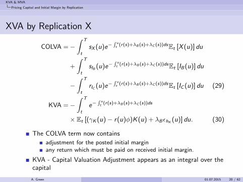
COLVA =−∫ T

t

sX (u)e−∫ ut

(r(s)+λB (s)+λC (s))dsEt [X (u)] du

+

∫ T

t

sIB (u)e−∫ ut

(r(s)+λB (s)+λC (s))dsEt [IB(u)] du

−∫ T

t

rIC (u)e−∫ ut

(r(s)+λB (s)+λC (s))dsEt [IC (u)] du (29)

KVA =−∫ T

t

e−∫ ut


× Et [(γK (u)− r(u)φ)K (u) + λBεhK (u)] du. (30)

The COLVA term now contains

adjustment for the posted initial marginany return which must be paid on received initial margin.

KVA - Capital Valuation Adjustment appears as an integral over thecapital

A. Green 01.07.2015 20 / 62

KVA & MVA


XVA by Replication XI

The FCA term contains the margin funding costs as we will nowdemonstrate.

Consider regular close-out + funding strategy = semi-replicationwith no shortfall on own-default (Burgard and Kjaer 2013).

2 issued bonds,

zero recovery bond, P1, used to fund Ubond with recovery R2 = RB +a hedge ratio given (7).

Hence we have,

α1P1 =− U (31)

α2P2 =− (V − φK − X + IB). (32)

Hedge error, εh, is given by

εh =gB + IB − X − φK + RBα2P2 (33)

=(1− RB)[(V − X + IB)+ − φK

]A. Green 01.07.2015 21 / 62

KVA & MVA


XVA by Replication XII

Hence we obtain the following for the valuation adjustment,

U = CVA + FVA + COLVA + KVA + MVA, (34)

where

CVA =− (1− RC )

∫ T

t

λC (u)e−∫ ut


× Et

[(V (u)− X (u)− IC (u))+

]du (35)

FVA =−∫ T

t

sF (u)e−∫ ut

(r(s)+λB (s)+λC (s))dsEt [(V (u)− X (u))] du

(36)

COLVA =−∫ T

t

sX (u)e−∫ ut

(r(s)+λB (s)+λC (s))dsEt [X (u)] du

−∫ T

t

rIC (u)e−∫ ut

(r(s)+λB (s)+λC (s))dsEt [IC (u)] du (37)

A. Green 01.07.2015 22 / 62

KVA & MVA


XVA by Replication XIII

KVA =−∫ T

t

e−∫ ut

(r(s)+λB (s)+λC (s))dsEt [K (u)(γK (u)− rB(u)φ)] du

(38)

MVA =−∫ T

t

(sF (u)− sIB (u))e−∫ ut

(r(s)+λB (s)+λC (s))dsEt [IB(u)] du,

(39)

where

sF (u) = (1− RB)λB(u)(V − X + IB)+ + (V − X + IB)− = (V − X + IB)

As expected, the MVA takes the form of an integral over theexpected initial margin profile.

We have grouped the change to the COLVA term with MVA as bothare determined by an integral over the initial margin profile.

In the one-sided IM case (CCP) the COLVA integral over IC is zero.

A. Green 01.07.2015 23 / 62

KVA & MVA

KVA Examples

KVA Examples I

Here are some example results to allow the impact of KVA to beassessed and compared to existing valuation adjustments.

Valuation adjustments were calculated using numeric integration ofthe XVA equations.

We choose to calculate the case of semi-replication with no shortfallat own default as described above.

A. Green 01.07.2015 24 / 62

KVA & MVA

KVA Examples

KVA Examples II

Assuming no initial margin the XVA becomes with regular bilateralcloseouts

CVA =− (1− RC )

∫ T

t

λC (u)e−∫ ut (λB (s)+λC (s))dsEt

[e−

∫ ut r(s)ds(V (u))+

]du

(40)

DVA =− (1− RB)

∫ T

t

λB(u)e−∫ ut (λB (s)+λC (s))dsEt

[e−

∫ ut r(s)ds(V (u))−

]du

(41)

FCA =− (1− RB)

∫ T

t

λB(u)e−∫ ut (λB (s)+λC (s))dsEt

[e−

∫ ut r(s)ds(V (u))+

]du

(42)

KVA =−∫ T

t

e−∫ ut (λB (s)+λC (s))dsEt

[e−

∫ ut r(s)dsK(u)(γK (u)− rB(u)φ)

]du,

(43)

A. Green 01.07.2015 25 / 62

KVA & MVA

KVA Examples

KVA Examples III

Since we consider an interest rate swap, interest rates are nowassumed to be stochastic so rates now appear inside expectations(The derivation follows the same steps as for derivatives based onstocks.)

A. Green 01.07.2015 26 / 62

KVA & MVA

KVA Examples

Setup

Market Risk: standardized approach with current exposure methodfor EAD

CCR: standardized approach with external ratings

CVA: large numbers of counterparties approximation. The use of thestandardized approaches avoids the complexity and bespoke natureof internal model methods.

Issuer holds the minimum capital ratio requirement of 10.5%(including minimum capital and capital buffer requirements) andthat the issuer cost of capital is 10%.

A. Green 01.07.2015 27 / 62

KVA & MVA

KVA Examples

Trade

Single 10 year GBP interest rate swap with semi-annual paymentschedules in both directions.

Fixed rate on the swap is 2.7% ensuring the unadjusted value is zeroat trade inception.

Issuer spread is flat 100bp across all maturities and the issuerrecovery rate is assumed to be 40%.

A. Green 01.07.2015 28 / 62

KVA & MVA

KVA Examples

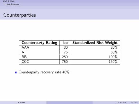
Counterparties

Counterparty Rating bp Standardized Risk WeightAAA 30 20%A 75 50%BB 250 100%CCC 750 150%

Counterparty recovery rate 40%.

A. Green 01.07.2015 29 / 62

KVA & MVA

KVA Examples

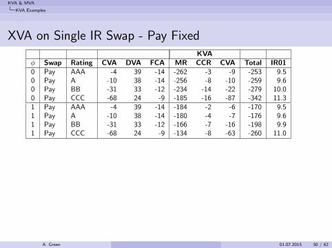
XVA on Single IR Swap - Pay FixedKVA

φ Swap Rating CVA DVA FCA MR CCR CVA Total IR010 Pay AAA -4 39 -14 -262 -3 -9 -253 9.50 Pay A -10 38 -14 -256 -8 -10 -259 9.60 Pay BB -31 33 -12 -234 -14 -22 -279 10.00 Pay CCC -68 24 -9 -185 -16 -87 -342 11.31 Pay AAA -4 39 -14 -184 -2 -6 -170 9.51 Pay A -10 38 -14 -180 -4 -7 -176 9.61 Pay BB -31 33 -12 -166 -7 -16 -198 9.91 Pay CCC -68 24 -9 -134 -8 -63 -260 11.0

A. Green 01.07.2015 30 / 62

KVA & MVA

KVA Examples

Setting aside the Market Risk component of the capital we see thatKVA from CCR and CVA terms gives an adjustment of similarmagnitude to the existing CVA, DVA and FCA terms, demonstratingthat KVA is a significant contributor to the price of the derivative.

Market risk is assumed to be unhedged and so this KVA componentis relatively large compared to the CCR and CVA terms.

Under the standardized approach to market risk the capitalrequirement on a ten year transaction of this type is scaled accordingto a 60 bp move in rates.

A. Green 01.07.2015 31 / 62

KVA & MVA

KVA Examples

When pricing derivatives it is no longer sufficient to look at theimpact of just the new trade, the impact of the trade and allhedging transactions should be considered.

The hedge trades will themselves create additional capitalrequirements, although they may also mitigate other capitalrequirements.

Consider a ten year interest rate swap traded with a corporate clienton an unsecured basis. This trade has market risk, counterpartycredit risk and CVA capital requirements associated with it.

To hedge the market risk the trading desk enters another ten yearswap with a market counterparty on a collateralised basis.

This hedge trade generates a small amount of counterparty creditrisk and CVA capital but reduces the market risk capita to zero as itis back-to-back with the client trade.

A. Green 01.07.2015 32 / 62

KVA & MVA

KVA Examples

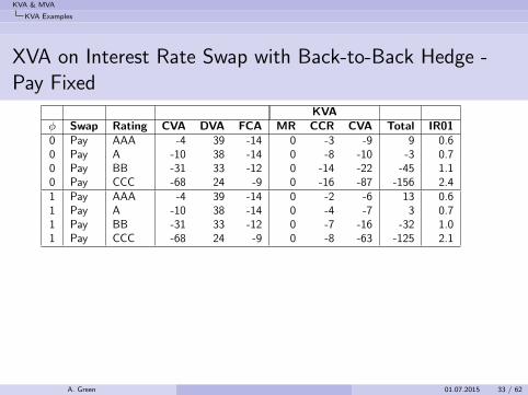
XVA on Interest Rate Swap with Back-to-Back Hedge -Pay Fixed

KVAφ Swap Rating CVA DVA FCA MR CCR CVA Total IR010 Pay AAA -4 39 -14 0 -3 -9 9 0.60 Pay A -10 38 -14 0 -8 -10 -3 0.70 Pay BB -31 33 -12 0 -14 -22 -45 1.10 Pay CCC -68 24 -9 0 -16 -87 -156 2.41 Pay AAA -4 39 -14 0 -2 -6 13 0.61 Pay A -10 38 -14 0 -4 -7 3 0.71 Pay BB -31 33 -12 0 -7 -16 -32 1.01 Pay CCC -68 24 -9 0 -8 -63 -125 2.1

A. Green 01.07.2015 33 / 62

KVA & MVA

KVA Examples

KVA itself, like CVA and FVA, has market risk sensitivities.

The CCR term, for example, is clearly driven by the EAD and henceby the exposure to the counterparty. Capital requirements go up asexposures rise irrespective to any impact on credit quality.

Reducing the IR01 of the trade and adjustments to zero yields thefollowing results

However, Market Risk Capital is no longer zero as trade and hedgeare not back-to-back.

A. Green 01.07.2015 34 / 62

KVA & MVA

KVA Examples

XVA on Interest Rate Swap - IR01 = 0 - Pay FixedKVA

φ Swap Rating CVA DVA FCA MR CCR CVA Total IR01 HedgeChange(%)

0 Pay AAA -4 39 -14 -17 -4 -12 -13 0 70 Pay A -10 38 -14 -20 -11 -13 -30 0 80 Pay BB -31 33 -12 -28 -20 -31 -88 0 120 Pay CCC -68 24 -9 -45 -22 -127 -249 0 241 Pay AAA -4 39 -14 -12 -3 -8 -1 0 61 Pay A -10 38 -14 -13 -5 -9 -14 0 71 Pay BB -31 33 -12 -18 -9 -23 -59 0 111 Pay CCC -68 24 -9 -29 -12 -92 -187 0 21

A. Green 01.07.2015 35 / 62

KVA & MVA

KVA Examples

Impact of KVA

KVA model = risk-neutral approach to pricing the cost of capital.

Clear that KVA really applies at Portfolio Level

’Hedging’ KVA will involve optimization / iteration as hedge tradeswill change KVA

Portfolio Level Effects - Leverage Ratio

KVA has other impacts:

’Exit Prices’Bank resolution planning - large portfolios = large leverage ratioimpact

A. Green 01.07.2015 36 / 62

KVA & MVA

Calculating MVA

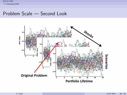
Scaling the Problem

104 trades per CCP Netting set

103 Monte Carlo paths

102 Observation points

102 − 103 Scenarios for VAR

104 × 103 × 102 × 103 = 1012

valuations...

A. Green 01.07.2015 37 / 62

KVA & MVA

Calculating MVA

Problem Scale — Second Look

Original Problem

Portfolio Lifetime

Scen

arios

A. Green 01.07.2015 38 / 62

KVA & MVA

Calculating MVA

VAR and the Risk-Neutral Measure

VAR is most commonly calculated using a historical simulationapproach and hence the VAR scenarios that are generated lie in thereal world measure.

From equation (39) it is clear that to proceed we need to applythese shocks inside a risk-neutral Monte Carlo simulation.

Here we choose to assume that the VAR shocks are exogenouslysupplied and that they do not change during the lifetime of theportfolio.

Allowing the shocks to change inside the risk-neutral Monte Carlowould mean combining the P and Q measures.

A. Green 01.07.2015 39 / 62

KVA & MVA

Calculating MVA

Longstaff-Schwartz Augmented Compression 1/2

To make VAR and CVAR calculations efficient the revaluation of the portfolio needs tobe very fast.Longstaff-Schwartz regression functions - simply a polynomial in the explanatoryvariables Oi (ω, tk) and hence very fast.Approximate value of the portfolio in each scenarios using regression functions with theexplanatory variables calculated using the shocked rates,

V Iq ≈ F (αm,Oi (y a

q , tk), tk). (44)

We apply the Longstaff-Schwartz approach to all derivative products from vanilla linearproducts to more complex exotic structures.Resulting regressions is also a compression technique.A single polynomial is used to replace the entire portfolio valuation.Longstaff-Schwartz Augmented Compression provides a portfolio valuation cost that isconstant and independent of portfolio size.Of course the regression phase of the calculation will itself be a function of the numberof cash flows in the portfolio but our results show that the computational costs isindependent of portfolio size in practice.

A. Green 01.07.2015 40 / 62

KVA & MVA

Calculating MVA

Longstaff-Schwartz Augmented Compression 2/2

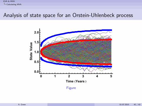
Longstaff-Schwartz, in its original form, requires augmentation for the VARand CVAR calculations because:

At t = 0 portfolio NPV has exactly 1 value, so regression is impossible.For t > 0 the state region explored by the state factor dynamics is muchsmaller than the region explored by VAR shocks.

Consider with a simple example where our model is driven by anOrstein-Uhlenbeck process (i.e. mean reverting),dx = η(µ− x)dt + σdW , x(0) = x0, where W is the driving Weiner process.Slide 1 shows the analysis of the state space with 1024 paths.It is clear that the 1024 paths shown do not cover the state space requiredby VAR calculation when the VAR shocks can give a shift of up to 30% on arelative basis.This magnitude of relative VAR shock was found in the 5-year time seriesused in the numerical examples presented below.

A. Green 01.07.2015 41 / 62

KVA & MVA

Calculating MVA

Analysis of state space for an Orstein-Uhlenbeck process

0 1 2 3 4 5

0.0

0.5

1.0

1.5

2.0

Time HYears L

Sta

teV

alu

e

Figure

A. Green 01.07.2015 42 / 62

KVA & MVA

Calculating MVA

Early Start Monte Carlo

There are two augmentation methods that we can apply, early start Monte Carloand shocked state augmentation.

Early Start Monte Carlo - starts the Monte Carlo simulation earlier thantoday so that enough Monte Carlo paths are present in the region required toobtain accurate regression results for VAR shocks.(Wang and Caflish 2009) suggested the use of early start Monte Carlo inorder to obtain sensitivities.The advantage of the early start Monte Carlo is that it preservespath-continuity.

This is needed for portfolios which contain American or Bermudan styleexercises.For such products a continuation value must be compared with an exercisevalue to obtain the correct valuation during the backward induction step.

Given the portfolios we will consider below contain only vanilla instrumentswe will not apply the early-start approach in this paper.

A. Green 01.07.2015 43 / 62

KVA & MVA

Calculating MVA

Shocked-State Augmentation 1/5

When portfolios do not contain American or Bermudan style exercisewe can use a simpler method to calculate regression functions givingportfolio values.

Typically the case for CCPs.

We call this approach Shocked-State Augmentation.

Simpler because it does not have to preserve path-continuity ofprices, as no backwards-induction step is required.

The regression at each stopping date is independent of of all otherregressions ⇒ parallel computation.

Objective is to have portfolio regressions that are accurate over therange of the state space relevant for calculation of VAR.

A. Green 01.07.2015 44 / 62

KVA & MVA

Calculating MVA


The dimensionality of the state space for VAR at any stopping date on any path isgiven by the dimensionality of a VAR shockOne VAR shock, for example, for a single interest rate may be described by 18 numbersgiving relative movements of the zero yield curve at different tenors, and hence be18-dimensional.The driving dimensionality is defined by the space explored by the VAR shocks.

Usually this will be larger than the dimensionality of the simulation model.This high-dimensionality must be explored by augmenting the state space.

At each stopping date the portfolio price is calculated as the sum of the componenttrades on each path.If there are m paths then this gives m values to fit.We can chose anything for the state variables (swaps and annuities in the example),and have as many as we like.We fit a regression connecting the portfolio value to the state variable values. Usuallym << n where n is the dimensionality of a VAR shock so the problem is overdetermined.We use a least-squares fit, so larger fitting errors are relatively highly penalized, underthe assumption that these are more likely to occur with more extreme scenarios.

A. Green 01.07.2015 45 / 62

KVA & MVA

Calculating MVA


We follow a parsimonious state augmentation strategy, that is completeat t=0. We assume that there are more simulation paths than VARshocks.

Shocked-State Augmentation: apply one VAR shock at eachstopping date, on each path.

This strategy is parsimonious because we do not require any extrasimulation paths, and because we use the same number of computationsas for a usual simulation (apart from computing the effect of the shockson the simulated data of course).

A. Green 01.07.2015 46 / 62

KVA & MVA

Calculating MVA


Strategy is complete at t=0 in that we are certain to cover the full rangerequired by VAR (as we have assumed more simulation paths than VARshocks).Automatic as we use the VAR shocks themselves to expand the state space.Hence certain that all VAR computations will be within the range over whichthe regressions were calibrated.Shocked-State Augmentation is the most parsimonious strategy in that ituses one VAR shock on each stopping date per simulation path.

In this version of Shocked-State Augmentation we pick the VAR shockssequentially for each path at each stopping date, So at t=1, say, path 1 usesshock 1, path 2 uses shock 2, etc.As we have more paths than shocks we will use some shocks multiple times.

A. Green 01.07.2015 47 / 62

KVA & MVA

Calculating MVA


Not interested in average effects of shocks — VAR is an extreme result ofthe shocks on the portfolio.Shocks cover a range of sizes (up to say 30% relative) it is not obviouswhich direction in the n-dimensional space (defined by VAR shockdimensionality) will have the biggest effect on the portfolio.Equally this is why we cannot simply pick the largest component of each ofthe VAR shocks and use this to expand the state space.Although a shock defined as the maximum component of each shock wouldbe large, we cannot say whether it is in the direction which changes theportfolio the most in n-dimensional space, for that magnitude of shock.In Shocked-State Augmentation the shocks are applied exactly as they wouldbe for computing VAR.

In our experiments interest rates VAR shocks are multiplicative shocks on zeroyield curve tenor points.They are applied in Shocked-State Augmentation just as they would be forVAR to create a new market data state (at each particular stopping date oneach path).

A. Green 01.07.2015 48 / 62

KVA & MVA

MVA: Numerical Examples


We calculate MVA on a series of portfolios of US Dollar interest rate swaps.We also calculate the FVA that would apply to the same portfolio if it wereunsecured in order to provide a reference calculation to assess the impact ofthe MVA.We assume the use of the following initial margin methodology,

99% one-sided VAR;10-day overlapping moves;5-year window including a period of significant stress. Our portfolio consistsof IRS so a suitable period starts January 2007.The 5-year window means that there were 1294 shocks.

Each VAR shock was a change to the zero yield curve.

Each VAR shock defined at 18 maturities: 0, 0.5 ,1 ,2 ,3 ,4 ,5 ,6 ,7 ,8 , 9, 10,11, 12, 15, 20, 25, 30 years.Shocks are relative changes to zero yields, so given a zero yield r at T and arelative shock s the resulting discount factor is: e−rT (1+s).Linear interpolation in yield between shock maturities.

A. Green 01.07.2015 49 / 62

KVA & MVA


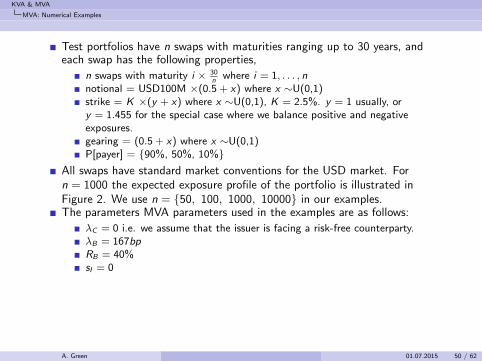
Test portfolios have n swaps with maturities ranging up to 30 years, andeach swap has the following properties,

n swaps with maturity i × 30n

where i = 1, . . . , nnotional = USD100M ×(0.5 + x) where x ∼U(0,1)strike = K ×(y + x) where x ∼U(0,1), K = 2.5%. y = 1 usually, ory = 1.455 for the special case where we balance positive and negativeexposures.gearing = (0.5 + x) where x ∼U(0,1)P[payer] = {90%, 50%, 10%}

All swaps have standard market conventions for the USD market. Forn = 1000 the expected exposure profile of the portfolio is illustrated inFigure 2. We use n = {50, 100, 1000, 10000} in our examples.The parameters MVA parameters used in the examples are as follows:

λC = 0 i.e. we assume that the issuer is facing a risk-free counterparty.λB = 167bpRB = 40%sI = 0

A. Green 01.07.2015 50 / 62

KVA & MVA


- 2,000 4,000 6,000 8,000

10,000 12,000 14,000

0 10 20 30

Exp

osu

re (

MU

SD)

Years

n=1,000

EPE

ENE

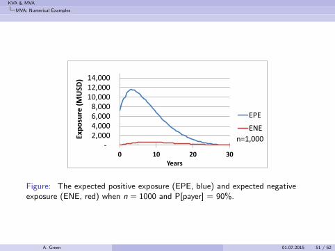
Figure: The expected positive exposure (EPE, blue) and expected negativeexposure (ENE, red) when n = 1000 and P[payer] = 90%.

A. Green 01.07.2015 51 / 62

KVA & MVA


Accuracy of Regression

0.0%0.5%1.0%1.5%2.0%2.5%3.0%

9 21 41 81

Erro

rs in

Re

gre

ssio

n

Po

rtfo

lio P

rice

s

Basis Size (#instruments)

n=1,000

mean

max

Very good with just a few basis functions.

Fewer basis functions are used at later times (because some of themhave matured)

A. Green 01.07.2015 52 / 62

KVA & MVA


Accuracy of VAR and ES

-30

-20

-10

0

10

50 100 1000 10000

Ave

rage

Err

or

in U

se

%/1

00

(b

asis

po

ints

)

Portfolio Size (#swaps)

#basis=41

Value

VAR

Funding

Better than pricing accuracy because of averaging effects — despitethe extreme nature of VAR and ES.

A. Green 01.07.2015 53 / 62

KVA & MVA


Speed

10

100

1,000

10,000

50

10

0

10

00

10

00

0

Co

mp

ute

Tim

e

(se

c)

Portfolio Size (#swaps)

#basis=41

Direct

Regression

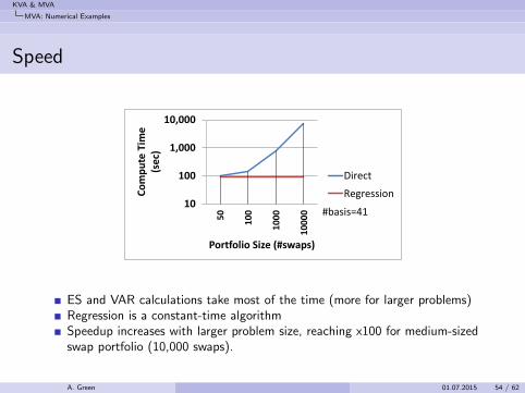
ES and VAR calculations take most of the time (more for larger problems)Regression is a constant-time algorithmSpeedup increases with larger problem size, reaching x100 for medium-sizedswap portfolio (10,000 swaps).

A. Green 01.07.2015 54 / 62

KVA & MVA


MVA Costs

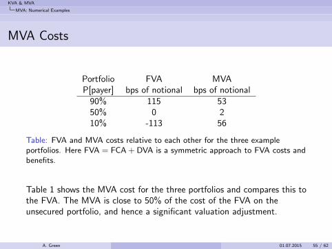
Portfolio FVA MVAP[payer] bps of notional bps of notional

90% 115 5350% 0 210% -113 56

Table: FVA and MVA costs relative to each other for the three exampleportfolios. Here FVA = FCA + DVA is a symmetric approach to FVA costs andbenefits.

Table 1 shows the MVA cost for the three portfolios and compares this tothe FVA. The MVA is close to 50% of the cost of the FVA on theunsecured portfolio, and hence a significant valuation adjustment.

A. Green 01.07.2015 55 / 62

KVA & MVA


Clearing: XVA vs MVA

Clearing: XVA vs MVA

The impact of clearing a portfolio of trades can be clearly seen nowthrough XVA

Cleared trades involve initial margin so MVA will be non-zero

The impact on the other XVAs will depend on the state prior toclearing

If no IM - C&FVA will likely reduce

KVA

Risk weight of CCP lowerBut leverage ratio impact less clear

Key Issue: Clearing decision involves optimization over XVA

Key Issue: CCP ’value’ is the reference value for margin not theeconomic value

A. Green 01.07.2015 56 / 62

KVA & MVA

KVA, MVA and Accounting

KVA, MVA and Accounting

Do KVA and MVA have accounting impact?

FVA now a part of accounting practice - 14 major banks now haveFVA reserves

FVA not in current Accounting StandardsFVA included on basis it is in the ’exit price’

Not clear what will happen to other valuation adjustments but see(Kenyon and Kenyon 2015).

A. Green 01.07.2015 57 / 62

KVA & MVA

Conclusions

Conclusions

Introduced KVA & MVA

Derived a risk-neutral model for KVA & MVA

Considered the numerical / market impact of KVA

Provided a numerical scheme to allow calculation of MVA

Assessed impact of MVA

A. Green 01.07.2015 58 / 62

KVA & MVA

Bibliography

Albanese, C., S. Caenazzo, and S. Iabichino (2015). Capital and Funding. SSRN.

BCBS-226 (2012). Margin requirements for non-centrally-cleared derivatives — consultativedocument. Basel Committee for Bank Supervision.

BCBS-242 (2013). Margin requirements for non-centrally cleared derivatives - Secondconsultative document. Basel Committee for Bank Supervision.

BCBS-261 (2013). Margin requirements for non-centrally cleared derivatives. Basel Committeefor Bank Supervision.

BCBS-317 (2015). Margin requirements for non-centrally cleared derivatives. Basel Committeefor Bank Supervision.

Burgard, C. and M. Kjaer (2013). Funding Strategies, Funding Costs. Risk 26(12).

Elouerkhaoui, Y. (2014). From fva to rwa: Should the cost of equity be included in the pricingof deals? Presented at Global Derivatives 2014.

Elouerkhaoui, Y. (2015). Kva the impact of rwa cost of capital on pricing. Presented at WBSCVA Conference 2015.

Green, A. (2015). XVA: Credit, Funding and Capital Valuation Adjustments. Wiley.Forthcoming.

Green, A. and C. Kenyon (2014). Portfolio KVA: I Theory. SSRN.http://ssrn.com/abstract=2519475.

A. Green 01.07.2015 59 / 62

http://ssrn.com/abstract=2519475

KVA & MVA

Bibliography

Green, A. and C. Kenyon (2015). MVA: Initial Margin Valuation Adjustment by Replication andRegression. Risk 28(5).

Green, A., C. Kenyon, and C. R. Dennis (2014). KVA: Capital Valuation Adjustment byReplication. Risk 27(12).

Hannah, L. (2014). A simple look at xvas (cva, dva, fca, kva). SSRN. Available at SSRN:http://ssrn.com/abstract=2471133.

Kenyon, C. and A. Green (2013). Pricing CDSs’ capital relief. Risk 26(10).

Kenyon, C. and A. Green (2014a, September). Regulatory costs break risk neutrality. Risk 27.

Kenyon, C. and A. Green (2014b, October). Regulatory costs remain. Risk 27.

Kenyon, R. and C. Kenyon (2015). Accounting for KVA Under IFRS 13. SSRN.http://ssrn.com/abstract=2620454.

Piterbarg, V. (2010). Funding beyond discounting: collateral agreements and derivativespricing. Risk 23(2), 97–102.

Piterbarg, V. (2012). Cooking with collateral. Risk 25(8), 58–63.

Piterbarg, V. (2013). Stuck with collateral. Risk 26(10).

Prampolini, A. (2014). The overlap of cva and capital requirements. Presented at 5th AnnualPractical CVA Forum.

Wang, Y. and R. Caflish (2009). Pricing and Hedging American-Style Options: A SimpleSimulation-Based Approach. Journal of Computational Finance 13(4), 95–125.

A. Green 01.07.2015 60 / 62

http://ssrn.com/abstract=2620454

KVA & MVA

Bibliography

Thanks for your attention — questions?

A. Green 01.07.2015 61 / 62

KVA & MVA

Bibliography

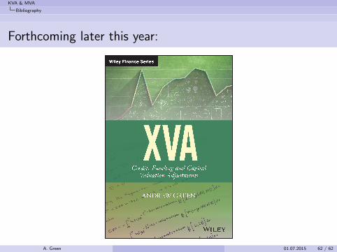
Forthcoming later this year:

A. Green 01.07.2015 62 / 62

kva and mva: capital valuation adjustment and margin ... · pdf filekva and mva: capital...

Documents