kshama thesis1 (repaired)
TRANSCRIPT

8/11/2019 Kshama Thesis1 (Repaired)
http://slidepdf.com/reader/full/kshama-thesis1-repaired 1/53
1
CHAPTER 1
INTRODUCTION
Black liquor is the spent liquid after the pulping process from the pulp mill. It is very complex,
contains high alkalinity and high dissolved solids such as lignin residues, degraded
carbohydrates and inorganic constituent. Black liquor is often called a waste although it contains
valuable energy and most importantly, converted expensive inorganic cooking chemicals. It is
conventionally burned in a large unit called Kraft recovery boiler. For the production of paper,
approximately 4 ton of wood, 200-250 kg chemicals & 8-10 ton of water are required which will
produce 1 ton of pulp and 10 ton of weak black liquor. If this liquor is treated it gives economic
and environmental benefits by way of:
Chemical recovery (caustic soda)
Energy recovery
Less pollution load
Unconventional energy production, from black liquor with surplus energy generation
Although the pulping chemical in the Kraft pulping process is only sodium hydroxide and
sodium carbonate, the discharging of this spent liquor/black liquor into the downstream without
proper treatment will definitely bring serious water pollution in term of biological oxygendemand (BOD), chemical oxygen demand (COD), total suspended solids (TSS), colour unit, pH,
odour and etc [1]. In the US, 80 million tons of black liquor (calculated for 25% water content
liquor) is burnt in recovery boilers every year. That corresponds to over 1% of the US total heat
and power generation [2]. In Northern Europe, black liquor plays even a more important role. In
Finland and Sweden black liquor combustion covers 7 and 4.5% of the total heat and power
generation, respectively. This corresponds in both cases to roughly 30% of the heat and power
generated from biofuels [3].

8/11/2019 Kshama Thesis1 (Repaired)
http://slidepdf.com/reader/full/kshama-thesis1-repaired 2/53
2
Recovery boiler have many problems including smelt-water explosions, unsteady smelt run off,
poor smelt reduction, low steam production, fouling of heat transfer tubes and plugging of flue
gas passages. So it is required to have a prior knowledge of kinetics of combustion of black
liquor when it is fired into the recovery boiler. Devolatilization is an important step in the
combustion of black liquor. Devolatilization refers to the rapid decomposition of organic
material into gaseous compounds and char. The devolatilization reactions affect the amount and
composition of black liquor char and the gas composition in the lower furnace.
Kinetic knowledge is of great importance in achieving good control of the combustion process
and in optimizing system design. Combustion model requires the proper understanding of
physical and chemical processes taking place in the particle during combustion. Kinetic model
should be developed that can predict the experimentally observed combustion behavior and can
be able to transfer experimental observations to furnace environment.
1.1.Outline of the Dissertation
Chapter 1 includes the brief introduction about the importance of Black liquor, how is it
generated and why is it necessary to the kinetics knowledge of devolatilization.
Chapter 2 gives the overview of pulping process and recovery section.
Chapter 3 includes the literature survey. In this chapter, the scenario of pulp and paper
industry has been discussed; black liquor composition and various models used for the
pyrolysis of black liquor are outlined.
Chapter 4 includes the experimental work performed for the purpose of study of
devolatilization of Black Liquor solids and also includes the results of neural network and
response surface methodology.
Chapter 5 includes the conclusion for the dissertation.

8/11/2019 Kshama Thesis1 (Repaired)
http://slidepdf.com/reader/full/kshama-thesis1-repaired 3/53
3
CHAPTER 2
PULPING PROCESS OVERVIEW
Wood is ground and pulped to separate the fibres from each other and to suspend the fibres in
water. Pulping breaks apart the wood fibres and cleans them of unwanted residues. In chemical
pulping, wood chips are cooked in an aqueous solution at high temperature and pressure.
Chemical processes dissolve most of the glue that holds the fibres together (lignin) while leaving
the cellulose fibres relatively undamaged. Chemical pulping produces a waste stream of
inorganic chemicals and wood residues known as black liquor . The Black liquor is concentrated
in evaporators and then incinerated in recovery furnaces, many of which are connected to steam
turbine cogeneration systems. The wood residues provide the fuel and the chemicals areseparated as smelt which is then treated to produce sodium hydroxide. In Figure 2.1 a simple
schematic description for the production of pulp and black liquor is shown.
Figure 2.1: Schematic representation of pulping process
8/11/2019 Kshama Thesis1 (Repaired)
http://slidepdf.com/reader/full/kshama-thesis1-repaired 4/53
4
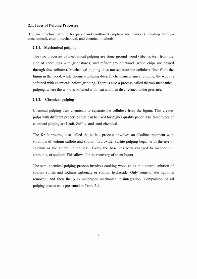
2.1.Types of Pulping Processes
The manufacture of pulp for paper and cardboard employs mechanical (including thermo-mechanical), chemi-mechanical, and chemical methods.
2.1.1.
Mechanical pulping
The two processes of mechanical pulping are stone ground wood (fiber is torn from the
side of short logs with grindstones) and refiner ground wood (wood chips are passed
through disc refiners). Mechanical pulping does not separate the cellulose fiber from the
lignin in the wood, while chemical pulping does. In chemi-mechanical pulping, the wood is
softened with chemicals before grinding. There is also a process called thermo-mechanical
pulping, where the wood is softened with heat and then disc-refined under pressure.
2.1.2.
Chemical pulping
Chemical pulping uses chemicals to separate the cellulose from the lignin. This creates
pulps with different properties that can be used for higher quality paper. The three types of
chemical pulping are Kraft, Sulfite, and semi-chemical.
The Kraft process, also called the sulfate process, involves an alkaline treatment with
solutions of sodium sulfide and sodium hydroxide. Sulfite pulping began with the use of
calcium as the sulfite liquor base. Today the base has been changed to magnesium,
ammonia, or sodium. This allows for the recovery of spent liquor.
The semi-chemical pulping process involves cooking wood chips in a neutral solution of
sodium sulfite and sodium carbonate or sodium hydroxide. Only some of the lignin is
removed, and then the pulp undergoes mechanical disintegration. Comparison of all
pulping processes is presented in Table 2.1.

8/11/2019 Kshama Thesis1 (Repaired)
http://slidepdf.com/reader/full/kshama-thesis1-repaired 5/53
5
Table 2.1 Comparison of the different types of pulping [4]
Kraft: chemical Sulfite: chemicalCTMP: chemi-
mechanical
Ground wood:
mechanical
yield of pulp 40-42% same as Kraft 90-92% about 80%
strength of
fibers
higher thanmechanical,lower than CTMP
lower than Kraft highest lowest strength
color/ brightness
more effective bleaching
methods have been developed
lower than Kraft high poor
cost
higher thanmechanical or
CTMP
lower than Kraftlower than
chemical
low
water use
depends on waterreuse, higher thanmechanical orCTMP
same as Kraftlower thanchemical
low
uses
fine paper, paperboard,
cartons,magazines, etc.
same as Kraft same as Kraft
low quality paper,newspaper,
tissues, towels,etc.
advantages
better than
Groundwood andsulfite, betterrecovery ofchemicals
better thanGroundwoodtechnique
less processingrequired, range ofwood species used
printing
disadvantages
toxic wastestreams (caused by bleaching,
odor
same as Kraft
highlyconcentratedeffluents, worse
than chemical
low strength,impermanent paper (reactive)

8/11/2019 Kshama Thesis1 (Repaired)
http://slidepdf.com/reader/full/kshama-thesis1-repaired 6/53
6
2.2.Chemical Recovery
For economic and environmental reasons, chemical and semi-chemical pulp mills employ
chemical recovery processes to reclaim spent cooking chemicals from the pulping process. At
Kraft and soda pulp mills, spent cooking liquor, referred to as “weak black liquor,” from the
brown stock washers is routed to the chemical recovery area at Kraft and soda pulp mills. The
chemical recovery process involves concentrating weak black liquor, combusting organic
compounds, reducing inorganic compounds, and reconstituting the cooking liquor. The typical
Kraft chemical recovery process consists of the general steps described in the following
paragraphs [5].
Black liquor concentration:
Residual weak black liquor from the pulping process is a dilute solution (approximately 12 to
15 percent solids) of wood lignins, organic materials, oxidized inorganic compounds (sodium
sulfate [Na2SO4], Na2CO3), and white liquor (Na2S and NaOH). The weak black liquor is first
directed through a series of multiple-effect evaporators (MEEs) to increase the solids content
to about 50 percent to form “strong black liquor.” The strong black liquor from the MEE
system is either oxidized in the black liquor oxidation (BLO) system if it is further
concentrated in a direct contact evaporator (DCE) or routed directly to a non-direct contact
evaporator (NDCE), also called a concentrator. Oxidation of the black liquor prior toevaporation in a DCE reduces emissions of odorous total reduced sulfur (TRS) compounds,
which are stripped from the black liquor in the DCE when it contacts hot flue gases from the
recovery furnace. The solids content of the black liquor following the final
evaporator/concentrator typically averages 65 to 80 percent [6].
Recovery furnace
The concentrated black liquor is then sprayed into the recovery furnace, where organic
compounds are combusted, and the Na2SO4 is reduced to Na2S. The black liquor burned in therecovery furnace has a high energy content (5,800 to 6,600 British thermal units per pound
[Btu/lb] of dry solids), which is recovered as steam for process requirements, such as cooking
wood chips, heating and evaporating black liquor, preheating combustion air, and drying the
pulp or paper products. The process steam from the recovery furnace is often supplemented
8/11/2019 Kshama Thesis1 (Repaired)
http://slidepdf.com/reader/full/kshama-thesis1-repaired 7/53
7
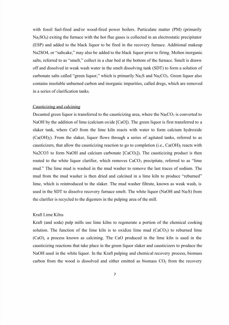
with fossil fuel-fired and/or wood-fired power boilers. Particulate matter (PM) (primarily
Na2SO4) exiting the furnace with the hot flue gases is collected in an electrostatic precipitator
(ESP) and added to the black liquor to be fired in the recovery furnace. Additional makeup
Na2SO4, or “saltcake,” may also be added to the black liquor prior to firing. Molten inorganic
salts, referred to as “smelt,” collect in a char bed at the bottom of the furnace. Smelt is drawn
off and dissolved in weak wash water in the smelt dissolving tank (SDT) to form a solution of
carbonate salts called “green liquor,” which is primarily Na2S and Na2CO3. Green liquor also
contains insoluble unburned carbon and inorganic impurities, called dregs, which are removed
in a series of clarification tanks.
Causticizing and calcining
Decanted green liquor is transferred to the causticizing area, where the Na2CO3 is converted to NaOH by the addition of lime (calcium oxide [CaO]). The green liquor is first transferred to a
slaker tank, where CaO from the lime kiln reacts with water to form calcium hydroxide
(Ca(OH)2). From the slaker, liquor flows through a series of agitated tanks, referred to as
causticizers, that allow the causticizing reaction to go to completion (i.e., Ca(OH)2 reacts with
Na2CO3 to form NaOH and calcium carbonate [CaCO3]). The causticizing product is then
routed to the white liquor clarifier, which removes CaCO3 precipitate, referred to as “lime
mud.” The lime mud is washed in the mud washer to remove the last traces of sod ium. The
mud from the mud washer is then dried and calcined in a lime kiln to produce “reburned”
lime, which is reintroduced to the slaker. The mud washer filtrate, known as weak wash, is
used in the SDT to dissolve recovery furnace smelt. The white liquor (NaOH and Na2S) from
the clarifier is recycled to the digesters in the pulping area of the mill.
Kraft Lime Kilns
Kraft (and soda) pulp mills use lime kilns to regenerate a portion of the chemical cooking
solution. The function of the lime kiln is to oxidize lime mud (CaCO3) to reburned lime
(CaO), a process known as calcining. The CaO produced in the lime kiln is used in the
causticizing reactions that take place in the green liquor slaker and causticizers to produce the
NaOH used in the white liquor. In the Kraft pulping and chemical recovery process, biomass
carbon from the wood is dissolved and either emitted as biomass CO2 from the recovery

8/11/2019 Kshama Thesis1 (Repaired)
http://slidepdf.com/reader/full/kshama-thesis1-repaired 8/53
8
furnace or captured in Na2CO3 exiting in the smelt from the recovery furnace. In the process
of converting the Na2CO3 into new pulping chemicals, this biomass carbon (i.e., the carbonate
ion) is transferred to CaCO3 in the causticizing process. In the lime kiln, the CaCO3 is
converted to CaO (i.e., lime material used in the chemical recovery process) and biomass CO2
originating from the wood residuals contained in black liquor is released to the atmosphere.
Figure 2.2 contains a simplified representation of the Kraft pulping and chemical recovery
process [7].
Figure 2.2: Simplified Representation of the Kraft Pulping and Chemical Recovery System
Unlike lime kilns used at lime production facilities, where CO 2 emissions are entirely fossil in
nature, the CO2 emitted from Kraft mill lime kilns originates from two sources:
(1) Fossil fuels burned in the kiln, and
(2) Conversion of CaCO3 (or “lime mud”) generated in the recovery process to CaO
(lime).
As shown above (in Figure 2.2), the calcium carbonate-derived CO2 emissions almost
exclusively originate from biomass. The lime kiln typically produces about 95 percent of the
lime needed for the causticizing reaction. Either make-up lime or limestone is purchased to
account for losses.
8/11/2019 Kshama Thesis1 (Repaired)
http://slidepdf.com/reader/full/kshama-thesis1-repaired 9/53
9
CHAPTER 3
LITERATURE SURVEY
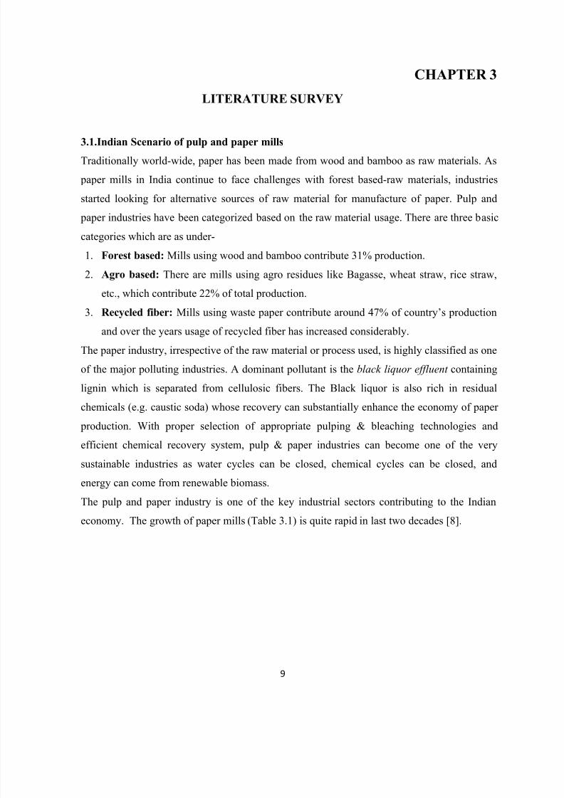
3.1.Indian Scenario of pulp and paper mills
Traditionally world-wide, paper has been made from wood and bamboo as raw materials. As
paper mills in India continue to face challenges with forest based-raw materials, industries
started looking for alternative sources of raw material for manufacture of paper. Pulp and
paper industries have been categorized based on the raw material usage. There are three basic
categories which are as under-
1. Forest based: Mills using wood and bamboo contribute 31% production.
2.
Agro based: There are mills using agro residues like Bagasse, wheat straw, rice straw,etc., which contribute 22% of total production.
3. Recycled fiber: Mills using waste paper contribute around 47% of country’s production
and over the years usage of recycled fiber has increased considerably.
The paper industry, irrespective of the raw material or process used, is highly classified as one
of the major polluting industries. A dominant pollutant is the black liquor effluent containing
lignin which is separated from cellulosic fibers. The Black liquor is also rich in residual
chemicals (e.g. caustic soda) whose recovery can substantially enhance the economy of paper
production. With proper selection of appropriate pulping & bleaching technologies and
efficient chemical recovery system, pulp & paper industries can become one of the very
sustainable industries as water cycles can be closed, chemical cycles can be closed, and
energy can come from renewable biomass.
The pulp and paper industry is one of the key industrial sectors contributing to the Indian
economy. The growth of paper mills (Table 3.1) is quite rapid in last two decades [8].
8/11/2019 Kshama Thesis1 (Repaired)
http://slidepdf.com/reader/full/kshama-thesis1-repaired 10/53
10
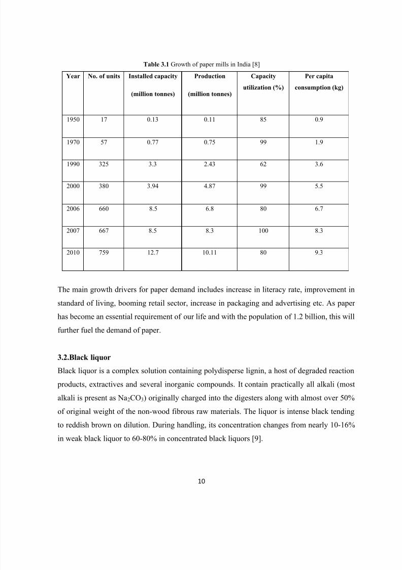
Table 3.1 Growth of paper mills in India [8]
Year No. of units Installed capacity
(million tonnes)
Production
(million tonnes)
Capacity
utilization (%)
Per capita
consumption (kg)
1950 17 0.13 0.11 85 0.9
1970 57 0.77 0.75 99 1.9
1990 325 3.3 2.43 62 3.6
2000 380 3.94 4.87 99 5.5
2006 660 8.5 6.8 80 6.7
2007 667 8.5 8.3 100 8.3
2010 759 12.7 10.11 80 9.3
The main growth drivers for paper demand includes increase in literacy rate, improvement in
standard of living, booming retail sector, increase in packaging and advertising etc. As paper
has become an essential requirement of our life and with the population of 1.2 billion, this will
further fuel the demand of paper.
3.2.Black liquor
Black liquor is a complex solution containing polydisperse lignin, a host of degraded reaction
products, extractives and several inorganic compounds. It contain practically all alkali (most
alkali is present as Na2CO3) originally charged into the digesters along with almost over 50%of original weight of the non-wood fibrous raw materials. The liquor is intense black tending
to reddish brown on dilution. During handling, its concentration changes from nearly 10-16%
in weak black liquor to 60-80% in concentrated black liquors [9].

8/11/2019 Kshama Thesis1 (Repaired)
http://slidepdf.com/reader/full/kshama-thesis1-repaired 11/53
11
Weak black liquor is Non-Newtonian in nature and has properties which influence its
transportation, heat transfer, combustion and stability. The properties are broadly given in the
following areas:
Rheological properties: density, viscosity
Thermal properties: specific heat, conductivity, foaming characteristics, boiling point rise
Combustion properties: ignition temperature, volatile matter calorific value, swelling
characteristics. The composition of black liquor is given in Table 3.1.
Table3.2 Elemental analysis of the dry black liquor solids [10]
Element w/w (%)
C 36.4
H 3.5
O 34.3
N 0.14
Na 18.6
K 2.02
Cl 0.24
S 4.8
total 100
From the point of view of fluid mechanics, black liquor is a liquid. However, it has two states,
fluid and solid. Its main components are inorganic cooking chemicals, lignin and other
organic constituents removed from the wood during pulping in the digester, and water. These
organic constituents are combined chemically with sodium hydroxide (NaOH) in the form of
sodium salts such as Na2S, Na2CO3 and Na2SO4. Table 3.3 shows a comparison of black
liquor, wood and two coals in terms of elemental composition and the most important
combustion properties that also affect the selection of a modeling approach.
8/11/2019 Kshama Thesis1 (Repaired)
http://slidepdf.com/reader/full/kshama-thesis1-repaired 12/53
12
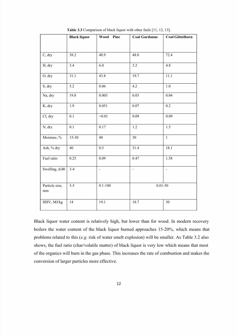
Table 3.3 Comparison of black liquor with other fuels [11, 12, 13].
Black liquor Wood Pine Coal Gardanne Coal Göttelborn
C, dry 38.2 48.9 48.0 72.4
H, dry 3.4 6.0 3.2 4.8
O, dry 31.1 43.8 19.7 11.1
S, dry 5.2 0.06 4.2 1.0
Na, dry 19.8 0.003 0.03 0.04
K, dry 1.9 0.051 0.07 0.2
Cl, dry 0.1 <0.01 0.09 0.09
N, dry 0.1 0.17 1.2 1.5
Moisture, % 15-30 40 30 1
Ash, % dry 40 0.5 31.4 18.1
Fuel ratio 0.25 0.09 0.47 1.58
Swelling, d/d0 3-4 - - -
Particle size,
mm
3-5 0.1-100 0.01-50
HHV, MJ/kg 14 19.1 18.7 30
Black liquor water content is relatively high, but lower than for wood. In modern recovery
boilers the water content of the black liquor burned approaches 15-20%, which means that
problems related to this (e.g. risk of water smelt explosion) will be smaller. As Table 3.2 also
shows, the fuel ratio (char/volatile matter) of black liquor is very low which means that most
of the organics will burn in the gas phase. This increases the rate of combustion and makes the
conversion of larger particles more effective.

8/11/2019 Kshama Thesis1 (Repaired)
http://slidepdf.com/reader/full/kshama-thesis1-repaired 13/53
13
Another important factor is the swelling behavior; the diameter of the particle may increase by
a factor of 3-4 during devolatilization. This effectively increases the external reaction surface
area, which affects the rate of external heat and mass transfer controlled processes. In the
recovery boiler, black liquor droplets are sprayed which do not keep their original shape
during swelling and in most of the modeling, spherical particles were considered [14]. From
the boiler operation point of view black liquor is a very difficult fuel as it has high ash content
and more importantly, black liquor ash has a very low melting point that may give rise to
severe boiler fouling problems [15].
3.3. Black liquor Gasification
In the pulp and paper industry, large quantities of forest biomass have been used and the by-
products or residues resulting from the industry including bark, forest logging residues and
black liquor are one of the major biomass resources that can be further used for energy
purpose to produce electricity, heat and bio fuels [16]. Black liquor gasification (BLG) is
considered as an alternative technology to replace conventional recovery cycle with the
recovery boiler. BLG technologies are distinguished in two major classes; (i) Low
temperature gasification, and (ii) High temperature gasification. Low temperature gasifier
operates at 600 – 850 oC, below the melting point of inorganics, thus avoiding smelt-water
explosions. High temperature gasification units generally operate in the 900 – 1000 oC range,
and produce a molten smelt [17].
3.4. Combustion of Black liquor
The combustion of black liquor has been studied for more than 40 years. Knowledge of the
composition of black liquor particles are required in order to study the combustion of the
black liquor in the boilers. A literature survey was conducted on the combustion stages of
black liquor. It is followed by explanation of different types of black liquor combustionmodels currently available to broaden the knowledge of the art of the modelling in this
category.The rapid development of numerical simulation methods has made it possible to
simulate a recovery furnace and accurately predict its performance [9] and has the potential to
enhance our understanding of the processes occurring in a recovery furnace.

8/11/2019 Kshama Thesis1 (Repaired)
http://slidepdf.com/reader/full/kshama-thesis1-repaired 14/53
14
Combustion of the organic portion of liquor in a recovery boiler will form sodium sulfide and
sodium carbonate and thus, produce heat. Then, the heat produces high pressure steam to
generate electricity and low pressure steam for process use. In order to convert the chemicals
and energy in the black liquor in an efficient way, the black liquor has to be atomized to
droplets and sprayed into the recovery unit in some way [18]. Typical representation of the
recovery boiler consists mainly of the furnace & several heat exchangers unit is shown in
figure 3.1.
Figure 3.1: Typical recovery furnace
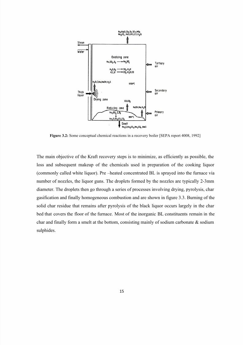
Figure 3.2 below shows some principal inorganic reactions in a recovery boiler and also
where in the furnace the reactions take place. In a conventional recovery boiler there is an
oxidizing zone in the upper part and a reducing zone in the lower part. The thick liquor is
introduced through one or several nozzles into the reducing zone. Combustion air is mostly
supplied at three different levels as primary, secondary and tertiary air (from the bottom up)
8/11/2019 Kshama Thesis1 (Repaired)
http://slidepdf.com/reader/full/kshama-thesis1-repaired 15/53
15
Figure 3.2: Some conceptual chemical reactions in a recovery boiler [SEPA report 4008, 1992]
The main objective of the Kraft recovery steps is to minimize, as efficiently as possible, the
loss and subsequent makeup of the chemicals used in preparation of the cooking liquor
(commonly called white liquor). Pre – heated concentrated BL is sprayed into the furnace via
number of nozzles, the liquor guns. The droplets formed by the nozzles are typically 2-3mmdiameter. The droplets then go through a series of processes involving drying, pyrolysis, char
gasification and finally homogeneous combustion and are shown in figure 3.3. Burning of the
solid char residue that remains after pyrolysis of the black liquor occurs largely in the char
bed that covers the floor of the furnace. Most of the inorganic BL constituents remain in the
char and finally form a smelt at the bottom, consisting mainly of sodium carbonate & sodium
sulphides.

8/11/2019 Kshama Thesis1 (Repaired)
http://slidepdf.com/reader/full/kshama-thesis1-repaired 16/53
16
Figure 3.3: Different stages of black liquor droplets in recovery boiler [19]
It has been understood that black liquor behaves in very unconventional fashion during
combustion. Its combustion behaviour is more like that of solid fuels, such as coal, than that
of oil or other liquid fuels. As the black liquor droplets enters the recovery unit they are being
exposed for hot gases and will undergo drying, pyrolysis, char conversion and smelt reaction.
During these stages the droplets undergo morphological changes which lead to changes in
both the heat transfer and aerodynamic properties of the droplets. In figure 3.4 these threemain stages are shown graphically.
Figure 3.4: Conversion stages of a black liquor droplet
The organic matter in black liquor solids begins to degrade thermally above 200 oC, producing
water vapor, CO2, CO, hydrogen, light hydrocarbons, tar, and light sulfur-containing gases

8/11/2019 Kshama Thesis1 (Repaired)
http://slidepdf.com/reader/full/kshama-thesis1-repaired 17/53
17
[20, 21]. For the relatively large (2-3 mm) droplets fired in black liquor burning,
devolatilization is essentially complete when the residue temperature reaches 650-750 C [22].
The char residue contains fixed carbon, some hydrogen, and most of the inorganic matter. The
following reactions very simply explain the combustion of the combustible organic
compounds:
C + O2 → CO2 + heat
2C + O2 → 2CO + heat
CO + ½O2 → CO2 + heat
2H2 + O2 → 2H2O + heat
In conjunction with the above combustion the following chemical reactions are also
occurring:
H2S + 1½O2 → SO2 + H2O
Na2O + SO2 + ½O2 → Na2SO4
NaOH + CO2 → Na2CO3 + H2O
Na2O + CO2→ Na2CO3
SO2 + ½O2 → SO3
The chemical transformation that takes place in the recovery boiler is not just due to
combustion, but also involves the reduction of sodium sulfate to sodium sulfide. The main
reaction is:
Na2SO4 + 2C + heat→ Na2S + 2CO2
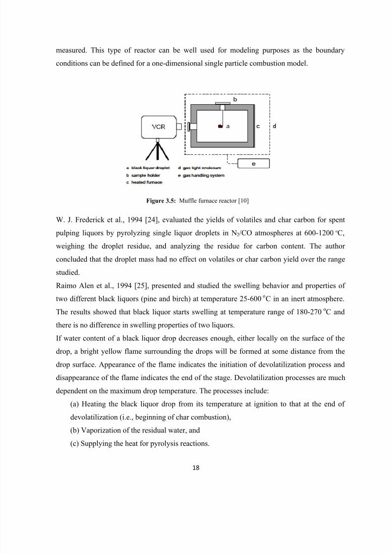
This reaction consumes heat, i.e. it is endothermic.For determining the combustion behavior of 1.5-2.5 mm particles, a muffle furnace, figure 3.5
has been extensively used [22, 23]. The duration of different combustion stages, swelling
behavior and mass loss and the release of species at predetermined time intervals are
8/11/2019 Kshama Thesis1 (Repaired)
http://slidepdf.com/reader/full/kshama-thesis1-repaired 18/53
18
measured. This type of reactor can be well used for modeling purposes as the boundary
conditions can be defined for a one-dimensional single particle combustion model.
Figure 3.5: Muffle furnace reactor [10]
W. J. Frederick et al., 1994 [24], evaluated the yields of volatiles and char carbon for spent
pulping liquors by pyrolyzing single liquor droplets in N2/CO atmospheres at 600-1200 oC,
weighing the droplet residue, and analyzing the residue for carbon content. The author
concluded that the droplet mass had no effect on volatiles or char carbon yield over the range
studied.
Raimo Alen et al., 1994 [25], presented and studied the swelling behavior and properties of
two different black liquors (pine and birch) at temperature 25-600 oC in an inert atmosphere.
The results showed that black liquor starts swelling at temperature range of 180-270 oC and
there is no difference in swelling properties of two liquors.
If water content of a black liquor drop decreases enough, either locally on the surface of the
drop, a bright yellow flame surrounding the drops will be formed at some distance from the
drop surface. Appearance of the flame indicates the initiation of devolatilization process and
disappearance of the flame indicates the end of the stage. Devolatilization processes are much
dependent on the maximum drop temperature. The processes include:
(a) Heating the black liquor drop from its temperature at ignition to that at the end of
devolatilization (i.e., beginning of char combustion),
(b) Vaporization of the residual water, and
(c) Supplying the heat for pyrolysis reactions.
8/11/2019 Kshama Thesis1 (Repaired)
http://slidepdf.com/reader/full/kshama-thesis1-repaired 19/53
19
Devolatilization time was taken as the duration of the visible flame and time needed to
complete above mentioned processes. The point of maximum swelling of the drop also
indicates the end of devolatilization stage.
During the devolatilization of black liquor droplets, investigation has been done on the factors
which influence the yield of volatiles and the carbon content of the char produced, i.e. liquor
type, droplet size, dry solid content, oxygen content, furnace temperature and pyrolysis time.
It was found that the amount of volatiles formed increased and the carbon content of the char
decreased with increasing reaction time at a constant furnace temperature. Carbon, sodium
and total mass loss from the char particles continued beyond devolatilization. This was
assumed to be due to sodium carbonate decomposition. The volatiles yield for different Kraft
liquor ranged from 35% to 47 % of the initial mass of the liquor [26].
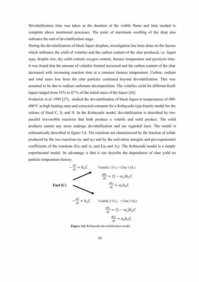
Frederick et al. 1999 [27], studied the devolatilization of black liquor at temperatures of 400-600°C at high heating rates and extracted constants for a Kobayashi-type kinetic model for the
release of fixed C, S, and N. In the Kobayashi model, devolatilization is described by two
parallel irreversible reactions that both produce a volatile and solid product. The solid
products cannot any more undergo devolatilization and are regarded inert. The model is
schematically described in figure 3.6. The reactions are characterized by the fraction of solids
produced by the two reactions (α1 and α2) and by the activation energies and pre-exponential
coefficients of the reactions (Ea1
and A1 and Ea
2and A
2). The Kobayashi model is a simple
experimental model. Its advantage is that it can describe the dependence of char yield on
particle temperature history.
Volatile 1 (V1) + Char 1 (S1)
Fuel (C)
Volatile 2 (V2) + Char 2 (S2)
Figure 3.6: Kobayashi devolatilization model

8/11/2019 Kshama Thesis1 (Repaired)
http://slidepdf.com/reader/full/kshama-thesis1-repaired 20/53
20
Hupa et al., 1994 [28], published an article on black liquor combustion in which they defined
the stages of black liquor combustion as drying, devolatilization and char burning. Their work
with a laboratory furnace enabled them to define three time-periods describing the entire
droplet combustion process: drying time, ti, from the initial contact with the gas to ignition;
devolatilization time, tv, from the appearance of the flame to maximum expansion; and char
burning time, tc. Good empirical correlations were established for all three: ti is proportional to
the initial droplet diameter, and both tv and tc are proportional to the 5/3 power of that
diameter. They were also able to generate profiles of the swelling and of the droplets
temperature as a function of the liquor combustion time.
As the combustion behaviour of black liquor is somewhat like of coal and other biomass so
kinetic model of devolatilization of coal and biomass were also studied.
A common approach in coal pyrolysis modeling is a single step nth order reaction. It assumes
that solid fuel, during one global decomposition step, transforms into solid residue (char) and
gaseous volatiles. The simplest of these models is the single 1st order model, which is popular
in engineering applications. For n = 1, the reaction rate is linearly dependent on the
concentration of the unreacted fuel. The single-step models are based on an empirical
expression of the global kinetics and do not describe the physical and chemical phenomena
taking place during pyrolysis. The rate of volatile release for reaction i is written as [29]:
( )
Here Vi,t is the volatile yield at time t, Vi,∞ the total volatile yield and n the reaction order. The
reaction rate coefficient K i is obtained from the well-known Arrhenius equation:
/RT)
The pre-exponential factor k i describes the probability that a collision between two molecules
leads to reaction. Ei is the activation energy and can be described as the height of an energy
8/11/2019 Kshama Thesis1 (Repaired)
http://slidepdf.com/reader/full/kshama-thesis1-repaired 21/53
21
barrier that must be overcome before the reaction can take place. R is the universal gas
constant and T temperature.
The modeling of coal pyrolysis has progressed from simple, (single equation) kinetic model to
complex "network" models. The most fundamental pyrolysis models, which try to describe the
physical and chemical phenomena taking place during devolatilization, are the network
models. These models approximate coal as a polymeric structure and provide more detailed
predictions of pyrolysis behavior than is possible with the simpler models. A total of three
network coal devolatilization models have been developed, [30-32], which have various
capacities for predicting coal thermal decomposition under practical conditions. These coal
devolatilization models are:
Functional Group - Depolymerization, Vaporization, Cross linking (FG-DVC) model
Chemical Percolation Devolatilization (CPD) model
FLASHCHAIN model
Belosevic et al., 2010 [33], indicated the importance of co-firing of coal with biomass which
can lead to CO2 reduction. In his study, different modelling approaches were reported for
different processes occurring during combustion of biomass.
3.5. Modelling techniques
A method for practical process modeling is the black box approach, where models are
obtained exclusively from experimental plant data. Such models do not provide a detailed
knowledge of the underlying physics of the problem, but they do provide a description of the
dynamic relationship between input and output variables. Statistical models based on
regression analysis are an example of such a black box approach. Recently a promising
modeling technique, artificial neural networks (ANNs) and response surface methodology
(RSM), has found numerous applications in representing the functional relationships between
input variables and the output (response) of the process using experimental data.

8/11/2019 Kshama Thesis1 (Repaired)
http://slidepdf.com/reader/full/kshama-thesis1-repaired 22/53
22
3.5.1. Artificial Neural Networks (ANNs)
In many situations, the functional relationship between covariates (also known as input
variables) and response variables (also known as output variables) is of great interest.
Artificial neural networks can be applied to approximate any complex functional
relationship. Neural network approach, unlike the mechanistic model, doesn’t require any
external manifestation of parametric relationship [34]. This makes artificial neural
networks a valuable statistical tool. Observed data are used to train the neural network
and the neural network learns an approximation of the relationship by iteratively adapting
its parameters. ANNs is built to train Multi-layer Perceptrons (MLP) in the context of
regression analyses, i.e. to approximate functional relationships between covariates and
response variables. Figure 3.7 shows the neural network topology with 4 inputs, 1 hidden
layer (15 neurons) and 1 output.
Figure 3.7: Neural Network topology
Fundamental aspects
The MLP is usually composed of an input, a hidden and an output layer of neurons. The
neurons in the input layer are typically linear, while the ones in the hidden layer have
nonlinear (often sigmoidal) activation functions. The neurons in the output layer may be
linear or nonlinear. Each interconnection between two layers of neurons has a parameter

8/11/2019 Kshama Thesis1 (Repaired)
http://slidepdf.com/reader/full/kshama-thesis1-repaired 23/53
23
associated with it that weights the feed forwardly passing signal. Additionally, each
neuron in the hidden and output layers has an intercept, also known as bias. Neural
networks are mainly characterized by the type of learning rule, neurons used and the way
that they are organized, number of layers and number of neurons per layer. These are
related to the number of training points and to the nature of the function [35]. The
learning algorithm is a procedure for modifying the weights and biases of the network.
Among the many leaning (training) algorithms of neural networks, the back propagation
(BP) has demonstrated excellent capability for various prediction and classification
problems [36]. Transfer functions for the neurons are needed/introduce to bring the non-
linearity into the network. Without this nonlinearity, neurons would behave in a linear
fashion and the ANN would not be able to account the nonlinear input-output
relationships. Now-a-days, three types of transfer function are being commonly used:Linear, Sigmoid and Tang hyperbolic [37].
Interpretability of statistical models, or the understanding of the way inputs relate to an
output in a model, is a desirable property in applied research. Commonly used models,
such as the logistic regression model, are interpretable, but often do not provide adequate
prediction, thus making their interpretation questionable. Statistical aspects of ANNs,
such as approximation and convergence properties, have been discussed, and compared
with properties of more classical methods [38, 39]. The large flexibility provided by
neural network models results in prediction with a relatively small bias, but a large
variance. Careful methods for variance control [40-42] can lead to a smaller prediction
error and are required to robustify the prediction.
3.5.2. Response Surface Methodology (RSM)
Response surface methodology (RSM) is a collection of mathematical and statistical
techniques for empirical model building. By careful design of experiments, the objective
is to optimize a response (output variable) which is influenced by several independent
variables (input variables). An experiment is a series of tests, called runs, in which
changes are made in the input variables in order to identify the reasons for changes in the
output response. The application of RSM to design optimization is aimed at reducing the
cost of expensive analysis methods (e.g. finite element method or CFD analysis) and their

8/11/2019 Kshama Thesis1 (Repaired)
http://slidepdf.com/reader/full/kshama-thesis1-repaired 24/53
24
associated numerical noise. In recent years, multivariate statistical techniques have been
preferred to identify the optimal combination of factors and interactions among factors,
which are not possible to identify using the univariate method. In addition, these
techniques are very useful tools to reduce the time and cost of studies. The experimental
design involves estimation of the coefficients in a mathematical model, predicting the
response, and checking the adequacy of the model [43].
Response Surface Methodology (RSM) combined with Artificial Neural Networks
(ANN) becomes a powerful tool for modeling and simulations for various processes.
Both methodologies don’t need the explicit expressions of the physical meaning of the
system or process under investigation.
Abbas et al., 2003 [44], presented the shortcomings of models for devolatilization,
combustion & emission and reported a new approach based on artificial neural network.Then neural network model was implemented with the existing 3D CFD combustion
code. Model based on neural network was found comparable with other devolatization
model and is fast, reliable for solving complex control problems.
Previous literature papers employed neural networks to predict characteristics of
combustion, pyrolysis or gasification processes. In reference [45], a hybrid gasification
model using ANNs was developed to estimate reactivity parameters of different types of
coal with relative success. Reference [46] used ANNs to predict the emission of pollutant
gases in the combustion process of a mixture of coal and urban solid residuals with a
good agreement between experimental and predicted data.
Joseph et al., [47] performed a comparison between classical statistical methods and
ANNs. They concluded that ANN models perform better than regression models and
show more tolerance to noise in the data.
Marchitan et al., 2010 [48], presents a comparative study between RSM and ANN for
reactive extraction optimization of tartaric acid from aqueous solution using amine. The
extraction efficiency was modeled and optimized as a function of three input variables,
i.e. tartaric acid concentration in aqueous phase, pH of aqueous solution and amine
concentration in organic phase. Both methodologies have been compared for their
modeling and optimization abilities. Both models have been employed for construction of

8/11/2019 Kshama Thesis1 (Repaired)
http://slidepdf.com/reader/full/kshama-thesis1-repaired 25/53
25
response/output surface plots in order to reveal the influence of input variables on
extraction efficiency as well as to figure out the interaction effects between variables.
To overcome the RSM at a disadvantage i.e. getting trapped in local minimum
(maximum), Babak Abbasi et al., 2012 [49], used neural networks as a means to improve
the estimation in the RSM. This approach leads to reducing the calculations.

8/11/2019 Kshama Thesis1 (Repaired)
http://slidepdf.com/reader/full/kshama-thesis1-repaired 26/53
26
CHAPTER 4
EXPERIMENTAL WORK
4.1.
Preparation of dry Black liquor solids (DBS)
Black liquor procured from a Star Paper Mills in Saharanpur after the evaporation and the
solid concentration is 62%. The black liquor sample was first heated and stirred to decrease
the viscosity and increase the homogeneity of the liquor. About 150 g of the liquor were
poured in a rectangular galvanized iron sheet of dimensions 35cm by 25 cm, and spread over
the sheet to form a thin film of liquor. This was necessary in order to increase the surface area,
shorten the drying time, and prevent non-uniformity in the liquor. Four sheets of liquor were
prepared with this method, and placed in a drying oven controlled at 105 °C for 12 hours to
evaporate the water content of black liquor, Figure 4-1. A thin dried layer of black liquor
remained on the sheet after drying and it was allowed to cool down to room temperature. The
weight of the sheet plus black liquor was noted periodically and when this weight reached a
constant value indicating that all the moisture had evaporated, the solids were scraped off. It
was powdered in a domestic mixer-grinder and sieved into different particle size ranges 63-90
µm.
4.2. Experiment using dry Black Liquor solids
For the experimental studies in the muffle furnace, a known amount of DBS was taken in a
standard silica crucible fitted with a lid. The crucible was purged with nitrogen and the initial
weight of the crucible & DBS noted. A laboratory muffle furnace (M/S Commercial
Equipments, New Delhi, India) fitted with kanthal aluminium heating elements, asbestos
lagging and digital temperature indicator/controller was used. Through a tiny hole in the door
of the muffle furnace, nitrogen (N2) gas was supplied to create an inert atmosphere in the
furnace. The furnace was heated up to the required temperature and the silica crucible quickly
inserted into the furnace using tongs. The crucible was kept in the muffle furnace for the
desired time period and then removed. To cool down the crucible to room temperature ice
quenching was done. The final weight of the cooled crucible was noted. An electronic
weighing balance (Sartorius GC16035-OCE, Germany) with an accuracy of 10 mg was used

8/11/2019 Kshama Thesis1 (Repaired)
http://slidepdf.com/reader/full/kshama-thesis1-repaired 27/53
27
for noting the weights. The range of the experimental parameters used in the study is given
below. Most of the experiments were replicated to verify the obtained results.
Temperature: 300 – 1000 oC
Holding time: 30 – 180 sec
Mass of DBS: 2 & 5 gms
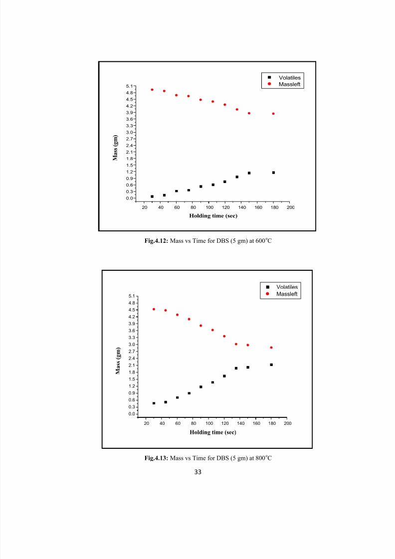
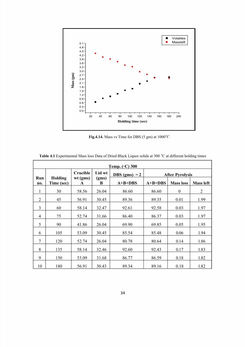
4.3. Experimental results obtained from the pyrolysis of dry Black Liquor solids
The experimental results obtained in the temperature range of 300oC-1000oC for different
time periods are shown in Figures 4.1-4.14 and the data is presented in Tables.
Fig.4.1: Mass vs Time for DBS (2 gm) at 300oC
20 40 60 80 100 120 140 160 180 200
0.0
0.2
0.4
0.6
0.8
1.0
1.2
1.4
1.6
1.8
2.0
M a s s ( g m )
Holding time (sec)
Volatiles
Massleft
8/11/2019 Kshama Thesis1 (Repaired)
http://slidepdf.com/reader/full/kshama-thesis1-repaired 28/53
28
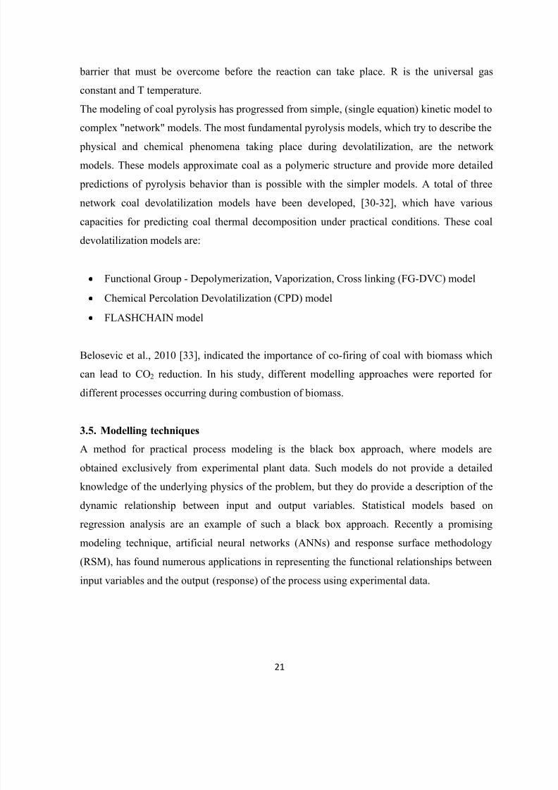
Fig.4.2: Mass vs Time for DBS (2 gm) at 400oC
Fig.4.3: Mass vs Time for DBS (2 gm) at 500oC
20 40 60 80 100 120 140 160 180 200
0.0
0.2
0.4
0.6
0.8
1.0
1.2
1.4
1.6
1.8
2.0
M a s s ( g m )
Holding time (sec)
Volatiles
Massleft
20 40 60 80 100 120 140 160 180 200
0.0
0.2
0.4
0.6
0.8
1.0
1.2
1.4
1.6
1.8
2.0
M a s s ( g m )
Holding time (sec)
Volatiles
Massleft

8/11/2019 Kshama Thesis1 (Repaired)
http://slidepdf.com/reader/full/kshama-thesis1-repaired 29/53
29
Fig.4.4: Mass vs Time for DBS (2 gm) at 600oC
Fig.4.5: Mass vs Time for DBS (2 gm) at 700oC
20 40 60 80 100 120 140 160 180 200
0.0
0.2
0.4
0.6
0.8
1.0
1.2
1.4
1.6
1.8
2.0
M a s s ( g m )
Holding time (sec)
Volatiles
Massleft
20 40 60 80 100 120 140 160 180 200
0.0
0.2
0.4
0.6
0.8
1.0
1.2
1.4
1.6
1.8
2.0
M a s s ( g m )
Holding time (sec)
Volatiles
Massleft
8/11/2019 Kshama Thesis1 (Repaired)
http://slidepdf.com/reader/full/kshama-thesis1-repaired 30/53
30
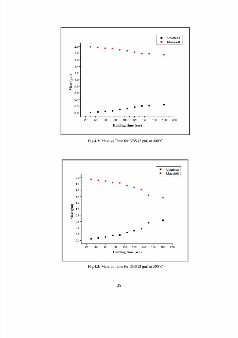
Fig.4.6: Mass vs Time for DBS (2 gm) at 800oC
Fig.4.7: Mass vs Time for DBS (2 gm) at 900oC
20 40 60 80 100 120 140 160 180 200
0.0
0.2
0.4
0.6
0.8
1.0
1.2
1.4
1.6
1.8
2.0
M a s s ( g m )
Holding time (sec)
Volatiles
Massleft
20 40 60 80 100 120 140 160 180 200
0.0
0.2
0.4
0.6
0.8
1.0
1.2
1.4
1.6
1.8
2.0
M a s s ( g m )
Holding time (sec)
Volatiles
Massleft
8/11/2019 Kshama Thesis1 (Repaired)
http://slidepdf.com/reader/full/kshama-thesis1-repaired 31/53
31
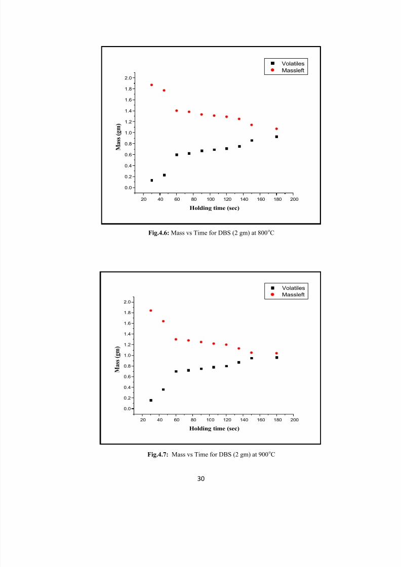
Fig.4.8: Mass vs Time for DBS (2 gm) at 1000oC
Fig.4.9: Mass vs Time for DBS (5 gm) at 300oC
20 40 60 80 100 120 140 160 180 200
0.0
0.2
0.4
0.6
0.8
1.0
1.2
1.4
1.6
1.8
2.0
M a s s ( g m )
Holding time (sec)
Volatiles
Massleft
20 40 60 80 100 120 140 160 180 200
0.0
0.3
0.6
0.9
1.2
1.5
1.8
2.1
2.4
2.7
3.0
3.3
3.6
3.9
4.2
4.5
4.8
5.1
M a s s ( g m )
Holding time (sec)
Volatiles
Massleft

8/11/2019 Kshama Thesis1 (Repaired)
http://slidepdf.com/reader/full/kshama-thesis1-repaired 32/53
32
Fig.4.10: Mass vs Time for DBS (5 gm) at 400oC
Fig.4.11: Mass vs Time for DBS (5 gm) at 500oC
20 40 60 80 100 120 140 160 180 200
0.0
0.3
0.6
0.9
1.2
1.5
1.8
2.1
2.4
2.7
3.0
3.3
3.6
3.9
4.2
4.5
4.8
5.1
M a s s ( g m )
Holding time (sec)
Volatiles
Massleft
20 40 60 80 100 120 140 160 180 200
0.0
0.3
0.6
0.9
1.2
1.5
1.8
2.1
2.4
2.7
3.0
3.3
3.6
3.9
4.2
4.5
4.8
5.1
M a s s ( g m )
Holding time (sec)
Volatiles
Massleft
8/11/2019 Kshama Thesis1 (Repaired)
http://slidepdf.com/reader/full/kshama-thesis1-repaired 33/53
33
Fig.4.12: Mass vs Time for DBS (5 gm) at 600oC
Fig.4.13: Mass vs Time for DBS (5 gm) at 800oC
20 40 60 80 100 120 140 160 180 200
0.0
0.3
0.6
0.9
1.2
1.5
1.8
2.1
2.4
2.7
3.0
3.3
3.6
3.9
4.2
4.5
4.8
5.1
M a s s ( g m )
Holding time (sec)
Volatiles
Massleft
20 40 60 80 100 120 140 160 180 200
0.0
0.3
0.6
0.9
1.2
1.5
1.8
2.1
2.4
2.7
3.0
3.3
3.6
3.9
4.2
4.5
4.8
5.1
M a s s ( g m )
Holding time (sec)
Volatiles
Massleft
8/11/2019 Kshama Thesis1 (Repaired)
http://slidepdf.com/reader/full/kshama-thesis1-repaired 34/53
34
Fig.4.14. Mass vs Time for DBS (5 gm) at 1000oC
Table 4.1 Experimental Mass loss Data of Dried Black Liquor solids at 300 oC at different holding times
Temp. (◦C) 300
Run
no.
Holding
Time (sec)
Crucible
wt (gms)
A
Lid wt
(gms)
B
DBS (gms) = 2 After Pyrolysis
A+B+DBS A+B+DBS Mass loss Mass left
1 30 58.56 26.04 86.60 86.60 0 2
2 45 56.91 30.45 89.36 89.35 0.01 1.99
3 60 58.14 32.47 92.61 92.58 0.03 1.97
4 75 52.74 31.66 86.40 86.37 0.03 1.97
5 90 41.86 26.04 69.90 69.85 0.05 1.95
6 105 53.09 30.45 85.54 85.48 0.06 1.94
7 120 52.74 26.04 80.78 80.64 0.14 1.868 135 58.14 32.46 92.60 92.43 0.17 1.83
9 150 53.09 31.68 86.77 86.59 0.18 1.82
10 180 56.91 30.43 89.34 89.16 0.18 1.82
20 40 60 80 100 120 140 160 180 200
0.0
0.3
0.6
0.9
1.2
1.5
1.8
2.1
2.4
2.7
3.0
3.3
3.6
3.9
4.2
4.5
4.8
5.1
M a s s ( g m )
Holding time (sec)
Volatiles
Massleft

8/11/2019 Kshama Thesis1 (Repaired)
http://slidepdf.com/reader/full/kshama-thesis1-repaired 35/53
35
Table 4.2 Experimental Mass loss Data of Dried Black Liquor solids at 400 oC at different holding times
Temp. (◦C) 400
Run
no.
Holding
Time (sec)
Crucible
wt (gms)
A
Lid wt
(gms)
B
DBS (gms) = 2 After Pyrolysis
A+B+DBS A+B+DBS Mass loss Mass left
1 30 58.55 31.67 92.22 92.21 0.01 1.99
2 45 52.76 26.04 80.80 80.77 0.03 1.97
3 60 56.92 30.46 89.38 89.33 0.05 1.95
4 75 53.06 30.42 85.48 85.42 0.06 1.94
5 90 58.53 26.04 86.57 86.47 0.10 1.90
6 105 41.85 32.45 76.30 76.17 0.13 1.87
7 120 52.76 31.68 86.44 86.27 0.17 1.838 135 58.09 26.04 86.13 85.92 0.21 1.79
9 150 41.82 30.43 74.25 74.03 0.22 1.78
10 180 53.09 32.52 87.61 87.36 0.25 1.75
Table 4.3 Experimental Mass loss Data of Dried Black Liquor solids at 500 oC at different holding times
Temp. (◦C) 500
Run
no.
Holding
Time (sec)
Crucible
wt (gms)
A
Lid wt
(gms) B
DBS (gms) = 2
After Pyrolysis
A+B+DBS A+B+DBS Mass loss Mass left
1 30 58.08 31.71 91.79 91.74 0.05 1.95
2 45 58.50 37.18 97.68 97.60 0.08 1.92
3 60 52.72 32.43 87.15 87.04 0.11 1.89
4 75 42.10 31.67 75.77 75.61 0.16 1.84
5 90 53.13 32.43 87.56 87.39 0.17 1.836 105 56.84 37.18 96.02 95.77 0.25 1.75
7 120 41.76 23.66 67.42 67.11 0.31 1.69
8 135 52.72 32.45 87.17 86.79 0.38 1.62
9 150 42.10 37.18 81.28 80.72 0.56 1.44
10 180 58.76 31.68 92.44 91.80 0.64 1.36

8/11/2019 Kshama Thesis1 (Repaired)
http://slidepdf.com/reader/full/kshama-thesis1-repaired 36/53
36
Table 4.4 Experimental Mass loss Data of Dried Black Liquor solids at 600 oC at different holding timee
Temp. (◦C) 600
Runno.
HoldingTime (sec)
Crucible
wt (gms)A
Lid wt
(gms) B
DBS (gms) = 2 After Pyrolysis A+B+DBS A+B+DBS Mass loss Mass left
1 30 53.13 32.47 87.60 87.54 0.06 1.94
2 45 58.57 26.04 86.61 86.50 0.11 1.89
3 60 52.73 37.18 91.91 91.79 0.12 1.88
4 75 58.07 32.46 92.53 92.37 0.16 1.84
5 90 56.87 30.42 89.29 88.97 0.32 1.68
6 105 41.80 37.18 80.98 80.40 0.58 1.42
7 120 42.15 32.47 76.62 75.96 0.66 1.34
8 135 53.15 26.04 81.19 80.48 0.71 1.29
9 150 58.09 30.43 90.52 89.78 0.74 1.26
10 180 52.74 24.58 79.32 78.51 0.81 1.19
Table 4.5 Experimental Mass loss Data of Dried Black Liquor solids at 700 oC at different holding times
Temp. (◦C) 700
Run
no.
HoldingTime
(sec)
Cruciblewt (gms)
A
Lid wt(gms)
B
DBS (gms) = 2 After Pyrolysis
A+B+DBS A+B+DBS Mass loss Mass left
1 30 52.62 32.43 87.05 86.95 0.10 1.9
2 45 42.06 31.65 75.71 75.59 0.12 1.88
3 60 53.08 37.17 92.25 91.90 0.35 1.65
4 75 41.75 26.02 69.77 69.35 0.42 1.58
5 90 58.48 26.04 86.52 86.06 0.46 1.54
6 105 58.01 31.67 91.68 91.04 0.64 1.36
7 120 42.09 37.18 81.27 80.55 0.72 1.28
8 135 58.02 32.47 92.49 91.72 0.77 1.23
9 150 52.73 32.46 87.19 86.39 0.80 1.20
10 180 41.78 31.19 74.97 74.13 0.84 1.16

8/11/2019 Kshama Thesis1 (Repaired)
http://slidepdf.com/reader/full/kshama-thesis1-repaired 37/53
37
Table 4.6 Experimental Mass loss Data of Dried Black Liquor solids at 800 oC at different holding times
Temp. (◦C) 800
Runno.
Holding Time (sec)
Crucible
wt (gms)A
Lid wt
(gms) B
DBS (gms) = 2 After Pyrolysis
A+B+DBS A+B+DBS Mass loss Mass left
1 30 42.12 31.69 75.81 75.68 0.13 1.87
2 45 56.83 26.03 84.86 84.63 0.23 1.77
3 60 52.74 30.44 85.18 84.58 0.60 1.4
4 75 53.10 21.96 77.06 76.44 0.62 1.38
5 90 52.71 32.46 87.17 86.50 0.67 1.33
6 105 41.78 32.45 76.23 75.54 0.69 1.31
7 120 58.07 37.18 97.25 96.54 0.71 1.29
8 135 42.13 23.69 67.82 67.07 0.75 1.25
9 150 56.84 30.43 89.27 88.41 0.86 1.14
10 180 53.13 31.70 86.83 85.90 0.93 1.07
Table 4.7 Experimental Mass loss Data of Dried Black Liquor solids at 900 oC at different holding times
Temp. (◦C) 900
Run
no. Holding
Time (sec)
Cruciblewt (gms)
A
Lid wt(gms)
B
DBS (gms) = 2 After Pyrolysis
A+B+DBS A+B+DBS Mass loss Mass left
1 30 58.55 30.42 90.97 90.81 0.16 1.84
2 45 58.08 31.69 91.77 91.41 0.36 1.64
3 60 41.82 23.69 67.51 66.81 0.70 1.30
4 75 56.87 24.58 83.45 82.73 0.72 1.28
5 90 52.75 26.04 80.79 80.04 0.75 1.25
6 105 53.15 32.46 87.61 86.83 0.78 1.227 120 41.82 23.69 67.51 66.71 0.80 1.2
8 135 58.56 32.45 93.01 92.14 0.87 1.13
9 150 42.14 30.42 74.56 73.61 0.95 1.05
10 180 58.11 31.66 91.77 90.65 1.12 0.88

8/11/2019 Kshama Thesis1 (Repaired)
http://slidepdf.com/reader/full/kshama-thesis1-repaired 38/53
38
Table 4.8 Experimental Mass loss Data of Dried Black Liquor solids at 1000 oC at different holding times
Temp. (◦C) 1000
Run
no.
Holding
Time (sec)
Crucible
wt (gms)
A
Lid wt
(gms)
B
DBS (gms) = 2 After Pyrolysis
A+B+DBS A+B+DBS Mass loss Mass left1 30 56.9 30.42 89.32 89.00 0.32 1.68
2 45 58.55 31.68 92.23 91.66 0.57 1.43
3 60 53.09 31.68 86.77 86.01 0.76 1.24
4 75 58.13 31.68 91.81 91.00 0.81 1.19
5 90 58.55 30.48 91.03 90.14 0.89 1.11
6 105 56.91 30.42 89.33 88.43 0.90 1.10
7 120 56.91 26.04 84.95 84.03 0.92 1.08
8 135 52.78 30.42 85.2 84.22 0.98 1.02
9 150 58.14 26.04 86.18 85.20 0.98 1.02
10 180 58.53 31.65 92.18 91.15 1.03 0.97
Table 4.9 Experimental Mass loss Data of Dried Black Liquor solids at 300 oC at different holding times
Temp. (◦C) 300
Runno.
Holding Time (sec)
Crucible
wt (gms)A
Lid wt
(gms) B
DBS (gms) = 5 After Pyrolysis
A+B+DBS A+B+DBS Mass loss Mass left
1 30 58.14 37.18 100.32 100.315 0.005 4.995
2 45 52.74 23.66 81.4 81.37 0.03 4.97
3 60 41.86 32.45 79.31 79.25 0.06 4.94
4 75 53.09 37.18 95.27 95.2 0.07 4.93
5 90 52.74 31.68 89.42 89.31 0.11 4.89
6 105 58.14 32.47 95.61 95.48 0.13 4.87
7 120 58.08 26.04 89.12 88.93 0.19 4.81
8 135 58.50 37.18 100.68 100.45 0.23 4.77
9 150 52.72 32.46 90.18 89.93 0.25 4.75
10 180 42.10 30.42 77.52 77.23 0.29 4.71
8/11/2019 Kshama Thesis1 (Repaired)
http://slidepdf.com/reader/full/kshama-thesis1-repaired 39/53
39
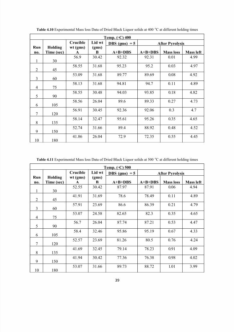
Table 4.10 Experimental Mass loss Data of Dried Black Liquor solids at 400 oC at different holding times
Temp. (◦C) 400
Run
no. Holding
Time (sec)
Crucible
wt (gms)
A
Lid wt
(gms) B
DBS (gms) = 5 After Pyrolysis
A+B+DBS A+B+DBS Mass loss Mass left
1 30 56.9 30.42 92.32 92.31 0.01 4.99
2 4558.55 31.68 95.23 95.2 0.03 4.97
3 6053.09 31.68 89.77 89.69 0.08 4.92
4 7558.13 31.68 94.81 94.7 0.11 4.89
5 9058.55 30.48 94.03 93.85 0.18 4.82
6 10558.56 26.04 89.6 89.33 0.27 4.73
7 12056.91 30.45 92.36 92.06 0.3 4.7
8 13558.14 32.47 95.61 95.26 0.35 4.65
9 15052.74 31.66 89.4 88.92 0.48 4.52
10 18041.86 26.04 72.9 72.35 0.55 4.45
Table 4.11 Experimental Mass loss Data of Dried Black Liquor solids at 500 oC at different holding times
Temp. (◦C) 500
Run
no. Holding
Time (sec)
Cruciblewt (gms)
A
Lid wt(gms) B
DBS (gms) = 5 After Pyrolysis A+B+DBS A+B+DBS Mass loss Mass left
1 3052.55 30.42 87.97 87.91 0.06 4.94
2 4541.91 31.69 78.6 78.49 0.11 4.89
3 6057.91 23.69 86.6 86.39 0.21 4.79
4 7553.07 24.58 82.65 82.3 0.35 4.65
5 9056.7 26.04 87.74 87.21 0.53 4.47
6 105 58.4 32.46 95.86 95.19 0.67 4.33
7 12052.57 23.69 81.26 80.5 0.76 4.24
8 13541.69 32.45 79.14 78.23 0.91 4.09
9 15041.94 30.42 77.36 76.38 0.98 4.02
10 18053.07 31.66 89.73 88.72 1.01 3.99
8/11/2019 Kshama Thesis1 (Repaired)
http://slidepdf.com/reader/full/kshama-thesis1-repaired 40/53
40
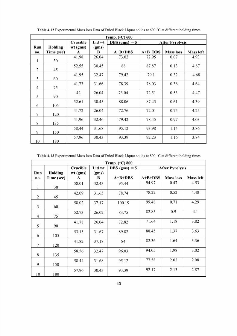
Table 4.12 Experimental Mass loss Data of Dried Black Liquor solids at 600 oC at different holding times
Temp. (◦C) 600
Run
no. Holding
Time (sec)
Crucible
wt (gms)
A
Lid wt
(gms) B
DBS (gms) = 5 After Pyrolysis
A+B+DBS A+B+DBS Mass loss Mass left
1 30 41.98 26.04 73.02 72.95 0.07 4.93
2 4552.55 30.45 88 87.87 0.13 4.87
3 6041.95 32.47 79.42 79.1 0.32 4.68
4 7541.73 31.66 78.39 78.03 0.36 4.64
5 9042 26.04 73.04 72.51 0.53 4.47
6 10552.61 30.45 88.06 87.45 0.61 4.39
7 12041.72 26.04 72.76 72.01 0.75 4.25
8 13541.96 32.46 79.42 78.45 0.97 4.03
9 15058.44 31.68 95.12 93.98 1.14 3.86
10 18057.96 30.43 93.39 92.23 1.16 3.84
Table 4.13 Experimental Mass loss Data of Dried Black Liquor solids at 800 oC at different holding times
Temp. (◦C) 800
Run
no.
Holding Time (sec)
Crucible
wt (gms)
A
Lid wt
(gms) B
DBS (gms) = 5 After Pyrolysis
A+B+DBS A+B+DBS Mass loss Mass left
1 3058.01 32.43 95.44 94.97 0.47 4.53
2 4542.09 31.65 78.74 78.22 0.52 4.48
3 6058.02 37.17 100.19 99.48 0.71 4.29
4 7552.73 26.02 83.75 82.85 0.9 4.1
5 9041.78 26.04 72.82 71.64 1.18 3.82
6 105
53.15 31.67 89.82 88.45 1.37 3.63
7 12041.82 37.18 84 82.36 1.64 3.36
8 13558.56 32.47 96.03 94.05 1.98 3.02
9 15058.44 31.68 95.12 77.58 2.02 2.98
10 18057.96 30.43 93.39 92.17 2.13 2.87

8/11/2019 Kshama Thesis1 (Repaired)
http://slidepdf.com/reader/full/kshama-thesis1-repaired 41/53
41
Table 4.14 Experimental Mass loss Data of Dried Black Liquor solids at 1000 oC at different holding times
Temp. (◦C) 1000
Run
no. Holding
Time (sec)
Crucible
wt (gms)
A
Lid wt
(gms) B
DBS (gms) = 5 After Pyrolysis
A+B+DBS A+B+DBS Mass loss Mass left
1 30 53.09 30.42 88.51 87.85 0.66 4.34
2 4558.13 31.69 94.82 93.88 0.94 4.06
3 6058.55 23.69 87.24 86.15 1.09 3.91
4 7556.91 24.58 86.49 85.21 1.28 3.72
5 9056.91 26.04 87.95 86.4 1.55 3.45
6 10552.78 32.46 90.24 88.57 1.67 3.33
7 120 58.08 23.69 86.77 84.72 2.05 2.95
8 13558.50 32.45 95.95 93.7 2.25 2.75
9 15052.72 30.42 88.14 85.63 2.51 2.49
10 18042.10 31.66 78.76 76.21 2.55 2.45
4.4. Modeling techniques for devolatilization of dry Black Liquor solids (DBS)
4.4.1. Artificial neural network (ANN) model
There are several ANN models such as feed-forward, Multi-Layer Perceptron (MLP) and the
Radial Basis Function (RBF) have been used in engineering applications to model or
approximate properties [50]. In this study, feed-forward MLP (with tangent sigmoid transfer
function (tansig) at hidden layers and at output layer were used as ANN network to predict the
volatiles release from the dry Black liquor solids during pyrolysis (Fig 4.15). The input- output
patterns required for training were obtained from experimental work. Different back-propagation
(BP) algorithms were compared to select the best suited BP algorithm. The Marquardt –
Levenberg learning algorithm with a minimum mean squared error (MSE) was found as the best.
The performance function for feed-forward networks is mean square error (MSE)- the average
squared error between the network outputs (a) and the target outputs (t). It is defined as follows:

8/11/2019 Kshama Thesis1 (Repaired)
http://slidepdf.com/reader/full/kshama-thesis1-repaired 42/53
42
The ANN model and its parameters variation were determined based on the minimum value ofthe MSE of the training and prediction set. The training parameters are used as number of input
nodes: 3, number of hidden neurons: 6, 10, and 15 number of output node: 1, learning rule:
Levenberg – Marquardt, number of epochs: 1000, error goal: 0.0001, Mu: 0.01 in this
investigation.
Fig 4.15: Neural network structure
In the ANN, 173 samples were taken for the training of the network by changing the number of
neurons whereas 72 samples were kept aside for the purpose of simulation. When the network
was sufficiently trained, 72 samples were then tested to see the how well the network is
predicting the values of unseen data. From fig 4.16 to 4.21, the results of test data and simulation
data for different neurons were shown. So from the comparison, 10 neurons in the hidden layer is
predicting the good results and it is well agreement with the experimental values. So the structure
of ANN used for modeling is 3 inputs, one hidden layer with 10 neurons, one output layer with 1
neuron and 1 output i.e. 3 x 10 x 1 x 1.

8/11/2019 Kshama Thesis1 (Repaired)
http://slidepdf.com/reader/full/kshama-thesis1-repaired 43/53
43
Fig 4.16: Output vs experimental values of 173 samples Fig 4.17: Actual vs predicted values of 72 samples (6(6 neuron) neuron)
Fig 4.18: Output vs experimental values of 173 samples Fig 4.19: Actual vs predicted values of 72 samples (10(10 neuron) neuron)
R² = 0.9647
0
0.5
1
1.5
2
2.5
3
0 1 2 3
Test data
R² = 0.7565
0
0.5
1
1.5
2
2.5
0 0.5 1 1.5
Simulation data
R² = 0.9505
0
0.5
1
1.5
2
2.5
3
0 1 2 3
Test data
R² = 0.9241
0
0.2
0.4
0.6
0.8
1
1.2
1.4
1.6
1.8
0 0.5 1 1.5
Simulation data

8/11/2019 Kshama Thesis1 (Repaired)
http://slidepdf.com/reader/full/kshama-thesis1-repaired 44/53
44
Fig 4.20: Output vs experimental values of 173 samples Fig 4.21: Actual vs predicted values of 72 samples (15
(15 neuron) neuron)
4.4.2. Response surface methodology (RSM) model
Box behnken design was used to understand the influence of the experimental factors and their
interactions on the release of volatile gases and to make predictions for different input values.
Tests were performed to investigate the factors affecting the mass loss of DBS. The levels of the
experimental factors and the design matrix are given in Table 4.15. The Box behnken had three
levels i.e. (-1, 0, +1) resulting in a total of 17 experiments used to optimize the chosen variables
for the mass loss. Experiments were performed in a random order, according to the below
experimental plan to avoid systematic errors.
R² = 0.9188
0
0.5
1
1.5
2
2.5
3
0 1 2 3
Test data
R² = 0.3701
0
0.5
1
1.5
2
2.5
3
0 0.5 1 1.5
Simulation data

8/11/2019 Kshama Thesis1 (Repaired)
http://slidepdf.com/reader/full/kshama-thesis1-repaired 45/53
45
Table 4.15 Experimental data set for Box behnken design
Factors Symbols
Level of factors
-1 0 1
Temperature (oC) X1 300 650 1000
Time (sec) X2 30 105 180
DBS (gm) X3 2 3.5 5
Run Actual and coded level of variables Mass loss (gm)
X1 X2 X3
1 -1 0 -1 0.062 0 1 1 0.65
3 0 -1 -1 0.084 1 0 -1 0.85 -1 1 0 0.556 -1 -1 0 0.017 0 1 -1 0.818 1 1 0 1.99 0 0 0 0.9810 0 0 0 1.0111 0 0 0 0.9812 0 0 0 0.9813 1 0 1 1.55
14 -1 0 1 0.1315 0 0 0 116 1 -1 0 0.617 0 -1 1 0.1
The experimental data was processed using Design Expert 9 Software. As can be seen from
Table 4.16, linear, square and interaction coefficients (X1X2) were found as significant terms at
the 5% probability level for the response mass loss.

8/11/2019 Kshama Thesis1 (Repaired)
http://slidepdf.com/reader/full/kshama-thesis1-repaired 46/53
46
Table 4.16 Estimated coefficients for Mass loss (gm) at coded units
Factor Coefficient Standard Error p-value
Intercept -0.010 0.098 < 0.0001
A-Temperature 1.30 0.078 < 0.0001
B-Time 1.17 0.078 < 0.0001
C-DBS 0.18 0.078 0.0464
AB -0.71 0.11 0.0001
A2 -0.53 0.11 0.0009
B2 -0.73 0.11 < 0.0001
C2 -0.62 0.11 0.0003
S = 0.22 R-Sq = 98.67% R-Sq(adj)= 97.64% PRESS = 2.51
According to the reduced quadratic model suggested by the RSM and recommended
transformation was natural logarithm, the relationship between the mass loss of DBS and the
factors was obtained with coded variables as follows:
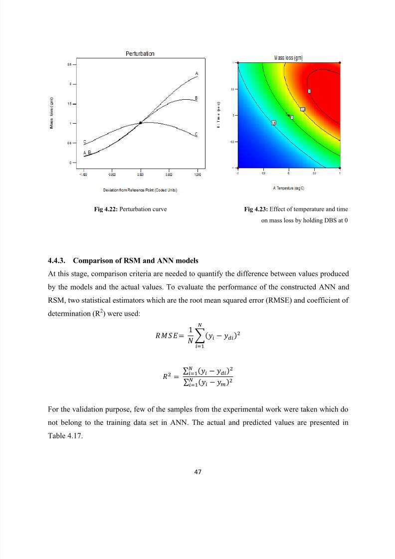
Fig 4.22 shows the effect of mass loss with the change in the variables (factors) within the
experimental range. So from the perturbation curve, it can be interpreted that temperature and
time are the significant variables which affect the release of volatiles during devolatilization.
This can also be justified by the equation given by the RSM that the intereaction of temperature
and time is the only interaction parameter which is affecting the mass loss. In the fig 4.23, effect
of temperature and time on the mass loss is shown and with the inrease in temperature and time,
relaese of volatiles is also significantly increasing.
8/11/2019 Kshama Thesis1 (Repaired)
http://slidepdf.com/reader/full/kshama-thesis1-repaired 47/53
47
Fig 4.22: Perturbation curve Fig 4.23: Effect of temperature and time
on mass loss by holding DBS at 0
4.4.3. Comparison of RSM and ANN models
At this stage, comparison criteria are needed to quantify the difference between values produced
by the models and the actual values. To evaluate the performance of the constructed ANN and
RSM, two statistical estimators which are the root mean squared error (RMSE) and coefficient of
determination (R 2) were used:
∑ ∑
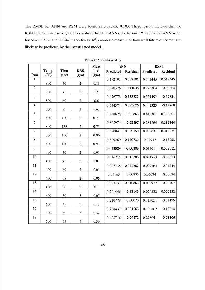
For the validation purpose, few of the samples from the experimental work were taken which do
not belong to the training data set in ANN. The actual and predicted values are presented in
Table 4.17.
8/11/2019 Kshama Thesis1 (Repaired)
http://slidepdf.com/reader/full/kshama-thesis1-repaired 48/53
48
The RMSE for ANN and RSM were found as 0.073and 0.103. These results indicate that the
RSMs prediction has a greater deviation than the ANNs prediction. R 2 values for ANN were
found as 0.9363 and 0.8942 respectively. R 2 provides a measure of how well future outcomes are
likely to be predicted by the investigated model.
Table 4.17 Validation data
Run
Temp.
(oC)
Time
(sec)
DBS
(gm)
Mass
loss
(gm)
ANN RSM
Predicted Residual Predicted Residual
1800 30 2 0.13
0.192101 0.062101 0.142445 0.012445
2800 45 2 0.23
0.340376 -0.11038 0.220364 -0.00964
3
800 60 2 0.6
0.476778 0.123222 0.321492 -0.27851
4800 75 2 0.62
0.534374 0.085626 0.442323 -0.17768
5800 120 2 0.71
0.738628 -0.02863 0.810361 0.100361
6800 135 2 0.75
0.808974 -0.05897 0.881864 0.131864
7800 150 2 0.86
0.820841 0.039159 0.905031 0.045031
8800 180 2 0.93
0.809269 0.120731 0.79947 -0.13053
9
400 30 2 0.01
0.013089 -0.00309 0.012011 0.002011
10400 45 2 0.03
0.016715 0.013285 0.021873 -0.00813
11400 60 2 0.05
0.027738 0.022262 0.037564 -0.01244
12400 75 2 0.06
0.05165 0.00835 0.06084 0.00084
13400 90 2 0.1
0.083137 0.016863 0.092927 -0.00707
14600 30 5 0.07
0.201446 -0.13145 0.070332 0.000332
16
600 45 5 0.130.210779 -0.08078 0.118051 -0.01195
17600 60 5 0.32
0.258437 0.061563 0.186862 -0.13314
18600 75 5 0.36
0.408716 -0.04872 0.278941 -0.08106

8/11/2019 Kshama Thesis1 (Repaired)
http://slidepdf.com/reader/full/kshama-thesis1-repaired 49/53
49
CHAPTER 5
CONCLUSION
RSM and ANN are modeling tools able to solve linear and nonlinear multivariate regression problems. RSM and ANN models were used to investigate the release of volatiles from dry black
liquor solids during pyrolysis process. Both models were well fitted to experimental data.
However, predictive power of ANN was found more powerful than that of CCD. On the other
hand, RSM has the advantage of giving a regression equation for prediction and showing the
effect of experimental factors and their interactions on response in comparison with ANN.
However, the main limitation of RSM assumes only quadratic non-linear correlation. Since ANN
can inherently capture almost any form of non-linearity, it can easily overcome limitation of
RSM. Another advantage of ANN is that this methodology does not require a standard
experimental design to build the model. In addition, an ANN model, unlike statistical models
operates upon the experimental data without data transformations.

8/11/2019 Kshama Thesis1 (Repaired)
http://slidepdf.com/reader/full/kshama-thesis1-repaired 50/53
50
REFERENCES
[1] Smook GA, Overview of pulping methodology, Handbook for Pulp & Paper Technologists,2nd edn. Angus Wilde Publications, Vancouver, (1992), pg 36.
[2] Macek, A., (1999) Research on combustion of black-liquor drops, Progress in Energy and
Combustion Science 25, (1999), pg 275.
[3] Asplund, D.,The Status and Development Possibilities of Bioenergy in Energy Industry,
Ministry of Trade and Industry, Energy Department, Finland, (1997).
[4] Sara Mortenson, BOD & COD in Effluent of Pulp and Paper Mills, retrived on 14-12-2013
[5] EPA, Pulp and Paper Combustion Sources National Emission Standards for Hazardous Air
Pollutants: A Plain English Description. U.S. Environmental Protection Agency. EPA-456/R-01-
003, (2001a). http://www.epa.gov/ttn/atw/pulp/chapters1-6pdf.zip
[6] EPA, Pulping and Bleaching System NESHAP for the Pulp and Paper Industry: A Plain
English Description. U.S. Environmental Protection Agency. EPA-456/R-01-002, (2001b).
Available: http://www.epa.gov/ttn/atw/pulp/guidance.pdf
[7] EPA, Technical Support Document for the Pulp and Paper Sector: Proposed Rule for
Mandatory Reporting of Greenhouse Gases. Office of Air and Radiation, U.S. EPA. February 11,
(2009c). Avaialble: http://www.epa.gov/climatechange/emissions/archived/ghg_tsd.html[8] GoI., Pulp and paper sector report of the working group for 12 th five year plan 2012-17.
Department of industrial Policy & Promotion of Commerce & industry, New Delhi, (2011), pp.
2-14
[9] Dr. Michalel J Kowerk, Properties of fibrous material and their preparation for pulping, Vol
1, Joint Textbook Committee, TAPPI, (1983), pp 154-164.
[10] M. Marklund. Black Liquor Recovery: How does it Work? (2011) Available:
http://www.etcpitea.se/blg/document/PBLG_or_RB. Pdf
[11] Adams, T. N., Frederick, J. M., Grace, T. M., Hupa, M., Iisa, K., Jones, A. K. and Tran, H.,
Kraft Recovery Boilers, Tappi Press, Atlanta, (1997)
[12] Kankkunen, A., Miikkulainen, P. and Järvinen, M., International Chemical Recovery
Conference, Whistler, BC, Canada, PAPTAC, Canada, (2001), pp 51-54

8/11/2019 Kshama Thesis1 (Repaired)
http://slidepdf.com/reader/full/kshama-thesis1-repaired 51/53
51
[13] Zevenhoven, R. and Hupa, M. Characterization of Solid Fuels for Advanced Pressurized
Combustion and Gasification, Proceedings of the 14th International Conference on Fluidized
Bed Combustion, ASME, New York, USA, 1997, (1997), pp. 213-227.
[14] Blasiak, W., Lixin, T., Vaclavinek J., “Recovery Furnace Modelling”, Preliminary study,
Nutek/IEA. Project no 92-09979, Department of Energy and Furnace Technology Stockholm,
Sweden, (1992).
[15] Hupa, M., Solin, P., Hyoty, P, Combustion behaviour of black liquor droplets, J. Pulp Paper
Science, 13(2), (1987), pp 67-72.
[16] Joelsson, J., Gustavsson, L., CO2 emission and oil use reduction through black liquor
gasification and energy efficiency in pulp and paper industry. Resources, Conservation and
Recycling 52, (2008), pp 747 – 763,.
[17] Patrick, K., Siedel, B., Gasification Edges Closer to Commercial reality with Three New N.A mills Startups. (2003).
[18] Green, R. P., Hough G., Chemical Recovery in the Alkaline Pulping Processes, ISBN 0-
8985-255-2, TP B-046, (1992)
[19] S. Ramesh, A. S. Chaurasia, H. Mahalingam, and N. J. Rao, Kinetics of Devolatilization of
Black Liquor Droplets in Chemical Recovery Boilers - Pyrolysis of Dry Black Liquor Solids, Int.
J. Chemical engineering and applications, 4, (2013)
[20] Kubes, G.J., Fleming, B.I., MacLeod, J.M., Bolker, H.I.,. Thermal analysis of spent pulping
liquor: activation energies. J. Wood Chem. Tech. 2 (3), (1982), pp 279-295.
[21] Bhattacharya, P., Vidyasekara, P., Kunzru, D., Pyrolysis of black liquor solids. Ind. Eng.
Chem. Proc. Des. Dev, 25, (1986), pp 420-426,.
[22] Frederick W. J. Hupa M, The Effects of Temperature and Gas Composition On Swelling of
Black Liquor Droplets During Devolatilization, Journal of Pulp and Paper Sci., 20, (1994), pp
274-280.
[23] Frederick, W. J., Combustion Processes in Black Liquor Recovery: Analysis and
Interpretation of Combustion Rate Data and an Engineering Model, DOE Report
DOE/CE/40637- T8, USA, (1990a).
[24] Frederick, W. J. and Hupa, M. Report 90-12, Gasification of Black Liquor at Elevated
Pressures, Part 2. Rate Data with CO2 and Water Vapor, Combustion Chemistry Research Group
Report, Åbo Akademi, Turku, Finland, (1990b).
8/11/2019 Kshama Thesis1 (Repaired)
http://slidepdf.com/reader/full/kshama-thesis1-repaired 52/53
52
[25] W. J. Frederick, M. Hupa & T. Uusikartano, Volatiles and char carbon yields during black
liquor pyrolysis, Bioresource Technology, 48, (1994), pp 59-64.
[26] Raimo Alen, Swelling behavior of kraft black liquor and its organic constituents,
Bioresource Technology 49, (1994), pp 99-103.
[27] Frederick, W. J., Hupa M., “Combustion Properties of Black Liquors“, US DOE Report
DOE/CE/40936-T1, (1993).
[28] Frederick, W.J., Phimolmas, V. and IISA K., “The Effect of Temperature and Residence
Time on the Distribution of Carbon, Sulfur and Nitrogen between Gaseous and Condensed Phase
Products from Low Temperature Pyrolysis of Kraft Black Liquor”, AIChE Symposium Series,
95, (1999), pp 119-127.
[29] R.H. Essenhigh. Fundamentals of coal combustion. In Chemistry of Coal Utilization, Ed.
M.A. Elliot, Wiley & Sons, (1981), pp 1153 – 1312.[30] Solomon, P. R., Hamblen, D. G., Carangelo, R. M., Serio, M. A,, and Deshpande, G. V.,
Energy & Fuels, 2,405 (1988).
[31] Solomon, P. R., Hamblen, D. G., Yu, Z. -Z. and Serio, M. A,, Fuel, 69, (1990), p 754.
[32] Solomon, P. R., Hamblen, D. G., Serio, M., A,, Yu, Z. -Z. and Charpenay, S. C., Fuel, 72,
(1993), p 469.
[33] Srdan Belosevic, Modeling Approaches to Predict Biomass Co-firing with Pulverized Coal,
the Open Thermodynamics Journal, 4, (2010), pp 50-70.
[34] P. McCullagh and J. Nelder. Generalized Linear Models. Chapman and Hall, London,
(1983).
[35] Shearer, S. A., J.A. Thomasson, T.G. Mueller, J.P. Fulton, S.F. Higgins and S. Samson,
Yield prediction using a neural network classifier trained using soil landscape features and soil
fertility dat. ASAE paper no. 993042. St. Joseph, Mich, (1999).
[36] Pao, Y.H., 1989. Adaptive Pattern Recognition and Neural networks. New York, Addison
Wesley, (1989).
[37] Ripley, B.D., Pattern Recognition and Neural Networks. Cambridge University Press, NY,
USA, (1996).
[38] Barron, A. R. and Barron, R. L., Statistical learning networks: A unifying view, in:
Wegman, E.,editor, Computing Science and Statistics: Proc. 20th Symp. Interface, American
Statistical Association, Washington, DC, (1988), pp 192-203.

8/11/2019 Kshama Thesis1 (Repaired)
http://slidepdf.com/reader/full/kshama-thesis1-repaired 53/53
[39] Geman, S., Bienenstock, E., and Doursat, R., Neural networks and the bias-variance
dilemma. Neural Computation, 4, (1992), pp 1-58.
[40] Barron, A. R., Complexity regularization with application to arti_cial neural networks, in:
Roussas, G., editor, Nonparametric Functional Estimation and Related Topics, (Kluwer
Academic Publishers, Dordrecht, The Netherlands, (1991), pp 561-576.
[41] Breiman, L., Bagging predictors. Machine Learning, 24, (1996), pp 123-140.
[42] Raviv, Y. and Intrator, N., Bootstrapping with noise: An effective regularization technique.
Connection Science, Special issue on combining Estimators, 8, (1996), pp 356-372.
[43] Montgomery, D.C., Design and Analysis of Experiments, seventh ed. John Wiley & Sons,
New York, (2008).
[44] T. Abbas, M.M. Awais, F.C. Lockwood, An artificial intelligence treatment of
devolatilization for pulverized coal and biomass in co-fired flames, Combustion and Flame 132,(2003), pp 305 – 318.
[45] Guo B., Shen Y., Li D., & Zhao F. Modelling coal gasification with a hybrid neural
network. Fuel, 76, (1997), pp 1159-1164.
[46] Dong C., Jin B., Zhong Z., & Lan J. Tests on co-firing of municipal solid waste and coal in
a circulating fluidized bed. Energy Conversion and Management, 43, (2002), pp 2189-2199.
[47] Joseph, B., Wang, F. H. and Shieh, D. S, Exploratory data analysis: A comparison of
statistical methods with artificial neural networks, Comp Chem Eng, 16, (1992), p 413.
[48] N. Marchitan, C. Cojocarub, A. Mereuta, Gh. Duca, I. Cretescu, M. Gonta, Modeling and
optimization of tartaric acid reactive extraction from aqueous solutions: A comparison between
response surface methodology and artificial neural network Separation and Purification
Technology 75, (2010), pp 273 – 285.
[49] Babak Abbasi, Hashem Mahlooji, Improving response surface methodology by using
artificial neural network and simulated annealing, Expert Systems with Applications 39, (2012),
pp 3461 – 3468.
[50] Haykin, S., Neural Networks: a Comprehensive Foundation, Second Edition.
Prentice Hall International, Inc, (1999).