ks chapter 5 fir filter design
DESCRIPTION
FIR FILTER DESIGNTRANSCRIPT

Chapter 5
FIR Filter Design
Objectives
• Describe the general approach to filter design and the design equation for FIR filters.
• Define phase distortion and show how it affects signals.• Demonstrate how linear phase response eliminates phase distortion.• Demonstrate the symmetry condition on FIR impulse response that results
in linear phase.• Derive the impulse responses of ideal low-pass and high-pass linear phase
filters.• Describe and demonstrate the window design method for linear phase FIR
filters.• Demonstrate the design of low-pass, high-pass, band-pass, and band-reject
FIR filters.• Describe and demonstrate the sampling method of linear phase FIR filter
design.• Demonstrate the tools in MATLAB for optimized FIR filter design using the
Parks-McClellan algorithm.
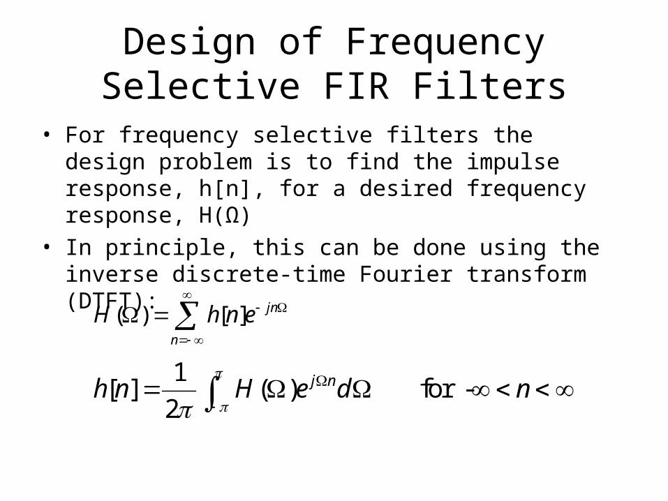
Design of Frequency Selective FIR Filters
• For frequency selective filters the design problem is to find the impulse response, h[n], for a desired frequency response, H(Ω)
• In principle, this can be done using the inverse discrete-time Fourier transform (DTFT):
1[ ] ( ) for -
2j nh n H e d n
( ) [ ] jn
n
H h n e
Phase Distortion
• Phase distortion results from a variable time delay (phase delay) for different frequency components of a signal.
• If the phase response of a filter is a linear function of frequency, then the phase delay is constant for all frequencies and no phase distortion occurs.
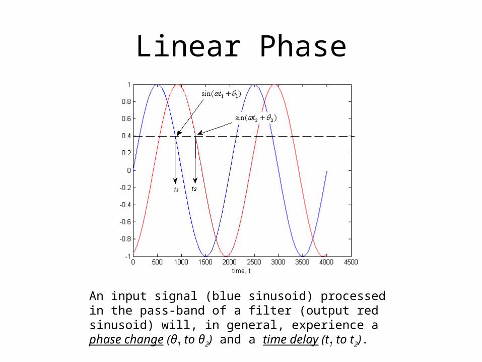
Linear Phase
An input signal (blue sinusoid) processed in the pass-band of a filter (output red sinusoid) will, in general, experience a phase change (θ1 to θ2) and a time delay (t1 to t2).
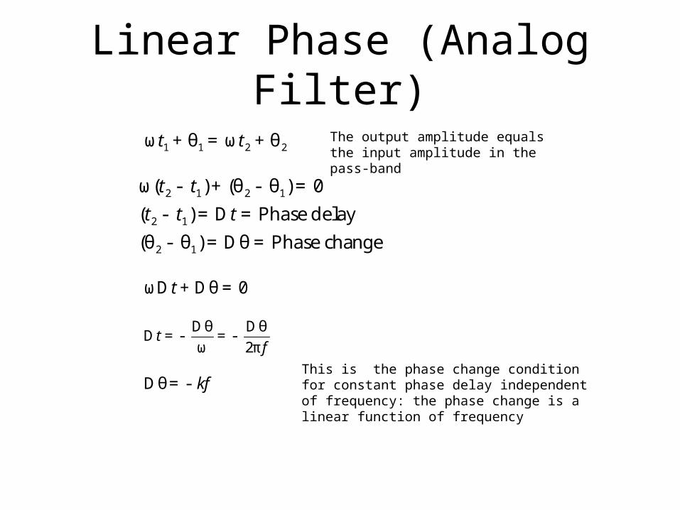
Linear Phase (Analog Filter)
1 1 2 2ω θ ω θt t+ = +
2 1 2 1
2 1
2 1
0ω( ) (θ θ )
( ) Phase delay
(θ θ ) θ Phase change
t t
t t t
- + - =
- =D =
- =D =
0ω θtD +D =
2
θ θω π
tf
D DD =- =-
θD =- kfThis is the phase change condition for constant phase delay independent of frequency: the phase change is a linear function of frequency
The output amplitude equals the input amplitude in the pass-band
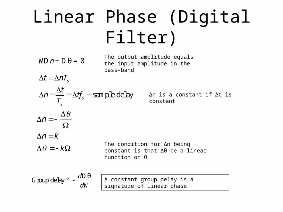
Linear Phase (Digital Filter)
sample delay
s
ss
t nT
tn tf
T
0θnWD +D =
n
n k
k
Δn is a constant if Δt is constant
The condition for Δn being constant is that Δθ be a linear function of Ω
The output amplitude equals the input amplitude in the pass-band
θGroup delay
Dº -
Wd
dA constant group delay is a signature of linear phase
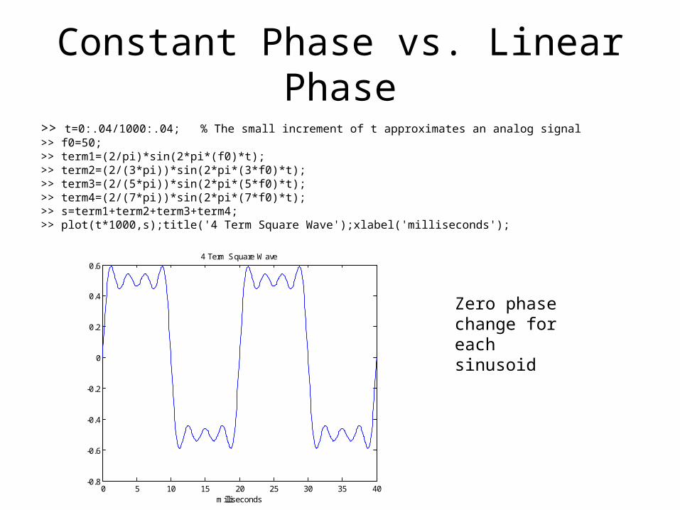
Constant Phase vs. Linear Phase
>> t=0:.04/1000:.04; % The small increment of t approximates an analog signal>> f0=50;>> term1=(2/pi)*sin(2*pi*(f0)*t);>> term2=(2/(3*pi))*sin(2*pi*(3*f0)*t);>> term3=(2/(5*pi))*sin(2*pi*(5*f0)*t);>> term4=(2/(7*pi))*sin(2*pi*(7*f0)*t);>> s=term1+term2+term3+term4;>> plot(t*1000,s);title('4 Term Square Wave');xlabel('milliseconds');
0 5 10 15 20 25 30 35 40-0.8
-0.6
-0.4
-0.2
0
0.2
0.4
0.64 Term Square Wave
milliseconds
Zero phase change for each sinusoid
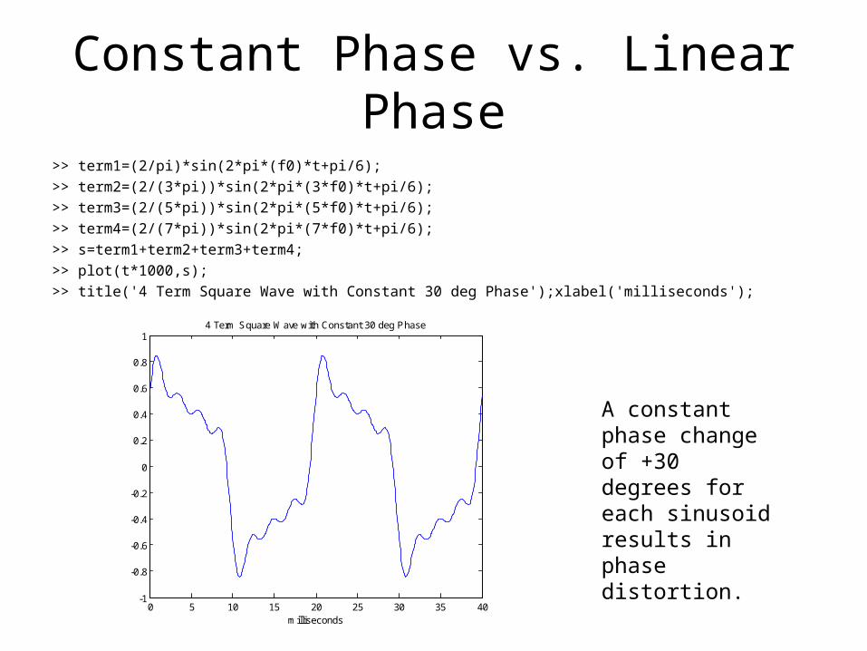
Constant Phase vs. Linear Phase
>> term1=(2/pi)*sin(2*pi*(f0)*t+pi/6);
>> term2=(2/(3*pi))*sin(2*pi*(3*f0)*t+pi/6);
>> term3=(2/(5*pi))*sin(2*pi*(5*f0)*t+pi/6);
>> term4=(2/(7*pi))*sin(2*pi*(7*f0)*t+pi/6);
>> s=term1+term2+term3+term4;
>> plot(t*1000,s);
>> title('4 Term Square Wave with Constant 30 deg Phase');xlabel('milliseconds');
0 5 10 15 20 25 30 35 40-1
-0.8
-0.6
-0.4
-0.2
0
0.2
0.4
0.6
0.8
14 Term Square Wave with Constant 30 deg Phase
milliseconds
A constant phase change of +30 degrees for each sinusoid results in phase distortion.
Constant Phase vs. Linear Phase
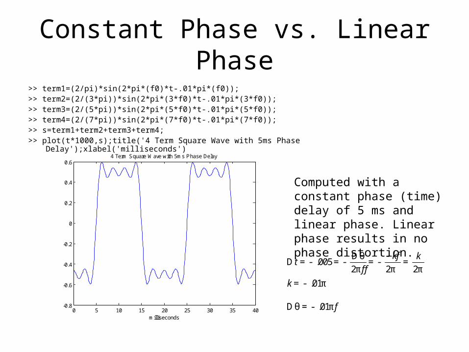
>> term1=(2/pi)*sin(2*pi*(f0)*t-.01*pi*(f0));>> term2=(2/(3*pi))*sin(2*pi*(3*f0)*t-.01*pi*(3*f0));>> term3=(2/(5*pi))*sin(2*pi*(5*f0)*t-.01*pi*(5*f0));>> term4=(2/(7*pi))*sin(2*pi*(7*f0)*t-.01*pi*(7*f0));>> s=term1+term2+term3+term4;>> plot(t*1000,s);title('4 Term Square Wave with 5ms Phase Delay');xlabel('milliseconds')
0 5 10 15 20 25 30 35 40-0.8
-0.6
-0.4
-0.2
0
0.2
0.4
0.64 Term Square Wave with 5ms Phase Delay
milliseconds
0052 2 2
θ.
π π πkf k
tff
-DD =- =- =- =
Computed with a constant phase (time) delay of 5 ms and linear phase. Linear phase results in no phase distortion.
01. πk=-
01θ . πfD =-

Sufficient Condition for Linear Phase
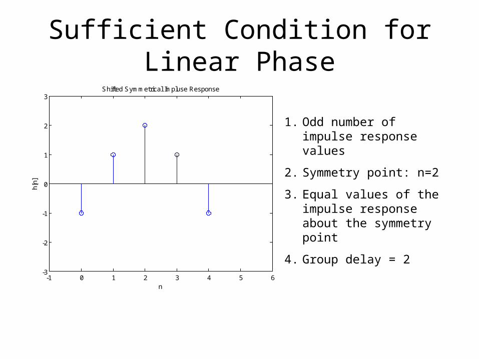
• If a FIR filter consists of an odd number of coefficients, M + 1, where M is even, and is symmetrical about the M/2 term, the filter has a linear phase response of Δθ = −(M/2)Ω. The filter will have a group delay of M/2
• This is termed a “type I” filter (odd length and positive symmetry). Other types have different permutations of length and symmetry. This type is the most common and easiest to design.
Sufficient Condition for Linear Phase
-1 0 1 2 3 4 5 6-3
-2
-1
0
1
2
3
n
h[n]
Shifted Symmetrical Impluse Response
1. Odd number of impulse response values
2. Symmetry point: n=2
3. Equal values of the impulse response about the symmetry point
4. Group delay = 2
Sufficient Condition for Linear Phase
0 0.1 0.2 0.3 0.4 0.5 0.6 0.7 0.8 0.90
0.9
1.8
2.7
3.6
4.5
Normalized Frequency ( rad/sample)
Mag
nitu
de
Magnitude and Phase Responses
-300
-240
-180
-120
-60
0
Pha
se (
degr
ees)
0 0.1 0.2 0.3 0.4 0.5 0.6 0.7 0.8 0.91
1.2
1.4
1.6
1.8
2
2.2
2.4
2.6
2.8
3
Normalized Frequency ( rad/sample)
Gro
up d
elay
(in
sam
ples
)
Group Delay
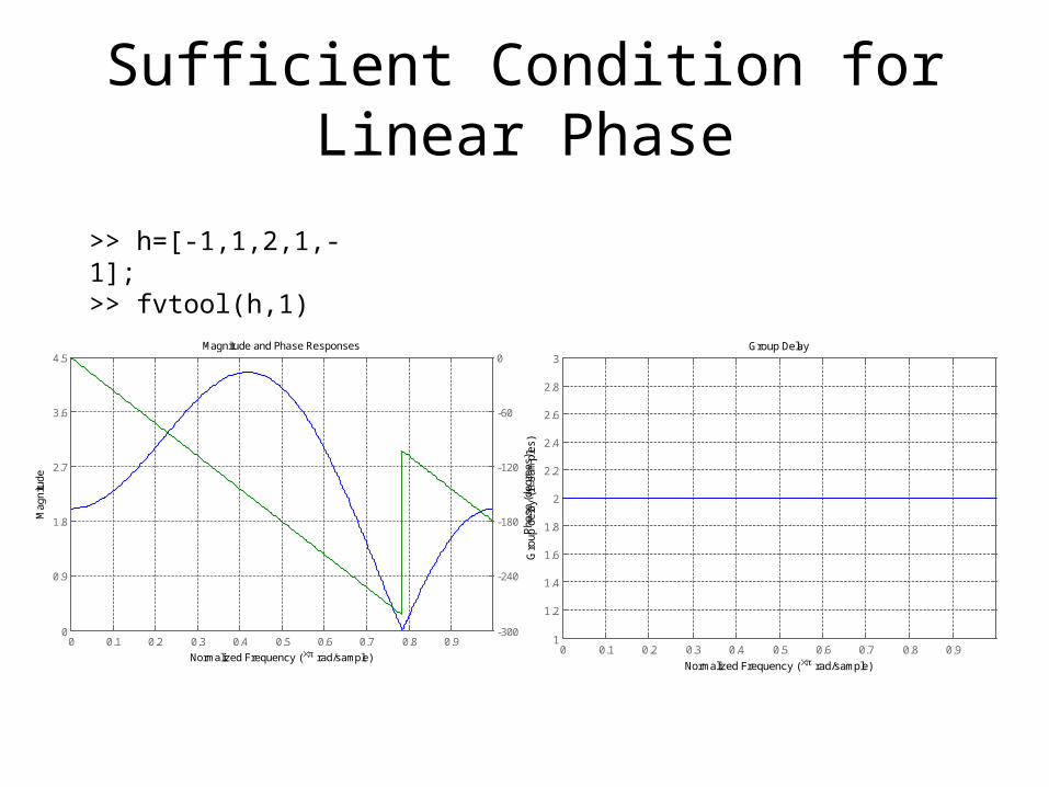
>> h=[-1,1,2,1,-1];>> fvtool(h,1)
Sufficient Condition for Linear PhaseThe Running Average Filter
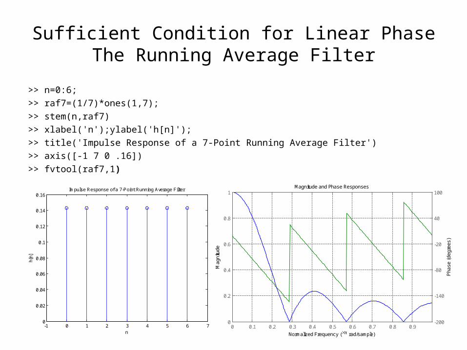
>> n=0:6;
>> raf7=(1/7)*ones(1,7);
>> stem(n,raf7)
>> xlabel('n');ylabel('h[n]');
>> title('Impulse Response of a 7-Point Running Average Filter')
>> axis([-1 7 0 .16])
>> fvtool(raf7,1)
-1 0 1 2 3 4 5 6 70
0.02
0.04
0.06
0.08
0.1
0.12
0.14
0.16
n
h[n]
Impulse Response of a 7-Point Running Average Filter
0 0.1 0.2 0.3 0.4 0.5 0.6 0.7 0.8 0.90
0.2
0.4
0.6
0.8
1
Normalized Frequency ( rad/sample)
Mag
nitu
de
Magnitude and Phase Responses
-200
-140
-80
-20
40
100
Pha
se (
degr
ees)
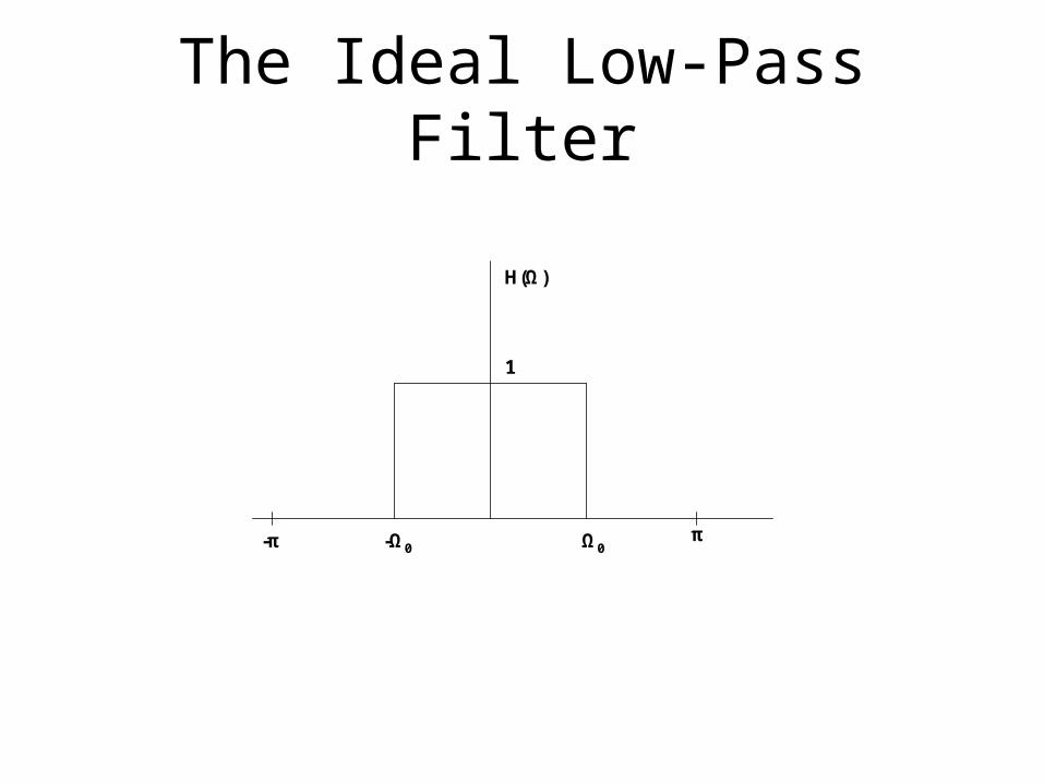
The Ideal Low-Pass Filter
Ω0-Ω0
H(Ω)
1
π-π
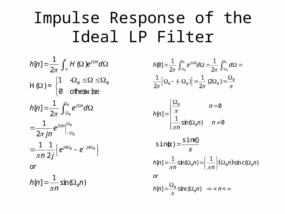
Impulse Response of the Ideal LP Filter
0
0
0
0
0 0
0 0
0
1[ ] ( )
21 -
H( ) = 0 otherwise
1[ ]
21
2
1 1
2
1[ ] sin( )
j n
j n
j n
jn jn
h n H e d
h n e d
ejn
e en j
or
h n nn
0 0
0 0
0
00 0 0
1 1[0]
2 21 1
( ) (2 )2 2
jh e d d
0
0
0[ ]
1sin( ) 0
nh n
n nn
x
xx
)sin()(sinc
0 0 0
00
1 1[ ] sin( ) sin c( )
[ ] sinc( ) -
h n n n nn n
or
h n n n
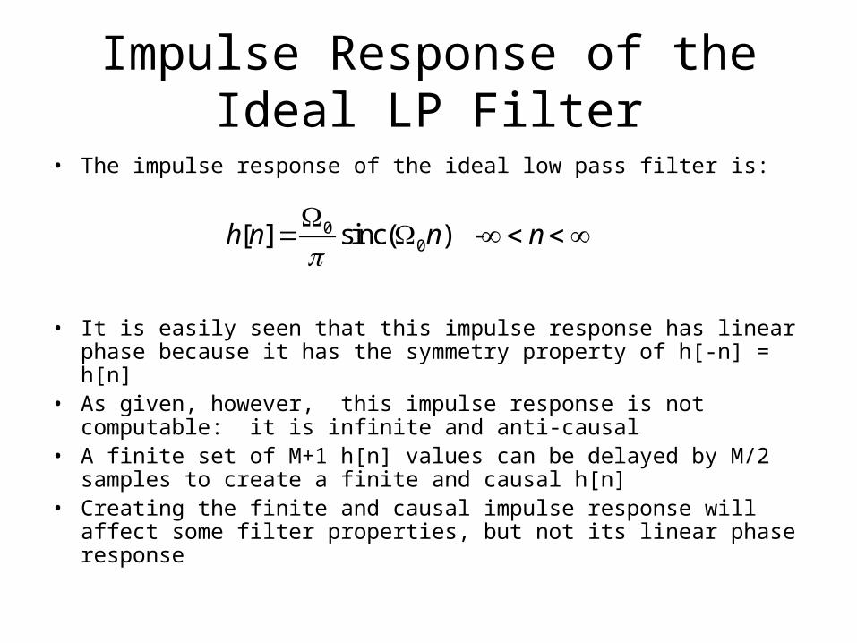
Impulse Response of the Ideal LP Filter
• The impulse response of the ideal low pass filter is:
• It is easily seen that this impulse response has linear phase because it has the symmetry property of h[-n] = h[n]
• As given, however, this impulse response is not computable: it is infinite and anti-causal
• A finite set of M+1 h[n] values can be delayed by M/2 samples to create a finite and causal h[n]
• Creating the finite and causal impulse response will affect some filter properties, but not its linear phase response
00[ ] sinc( ) - h n n n
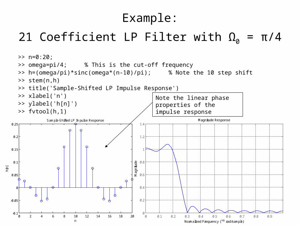
Example:
21 Coefficient LP Filter with Ω0 = π/4 >> n=0:20; >> omega=pi/4; % This is the cut-off frequency>> h=(omega/pi)*sinc(omega*(n-10)/pi); % Note the 10 step shift>> stem(n,h)>> title('Sample-Shifted LP Impulse Response')>> xlabel('n')>> ylabel('h[n]')>> fvtool(h,1)
0 2 4 6 8 10 12 14 16 18 20-0.1
-0.05
0
0.05
0.1
0.15
0.2
0.25Sample-Shifted LP Impulse Response
n
h[n]
0 0.1 0.2 0.3 0.4 0.5 0.6 0.7 0.8 0.90
0.2
0.4
0.6
0.8
1
1.2
1.4
Normalized Frequency ( rad/sample)
Mag
nitu
de
Magnitude Response
Note the linear phase properties of the impulse response
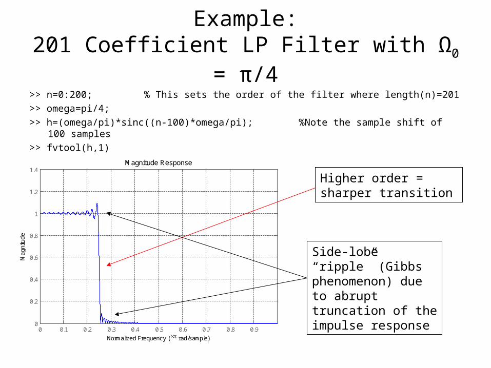
Example:201 Coefficient LP Filter with Ω0 = π/4
>> n=0:200; % This sets the order of the filter where length(n)=201
>> omega=pi/4;
>> h=(omega/pi)*sinc((n-100)*omega/pi); %Note the sample shift of 100 samples
>> fvtool(h,1)
0 0.1 0.2 0.3 0.4 0.5 0.6 0.7 0.8 0.90
0.2
0.4
0.6
0.8
1
1.2
1.4
Normalized Frequency ( rad/sample)
Mag
nitu
de
Magnitude Response
Higher order = sharper transition
Side-lobe “ripple” (Gibbs phenomenon) due to abrupt truncation of the impulse response
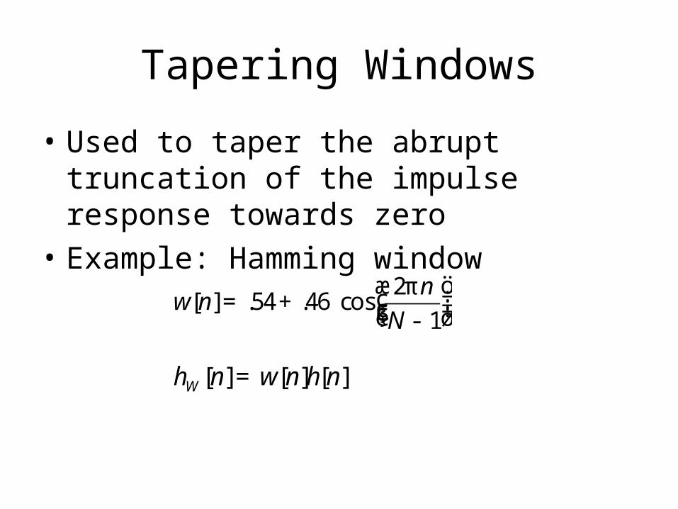
Tapering Windows
• Used to taper the abrupt truncation of the impulse response towards zero
• Example: Hamming window
254 46
1
π[ ] . . cos
nwn
Næ ö÷ç= + ÷ç ÷çè ø-
[ ] [ ] [ ]Wh n wnhn=
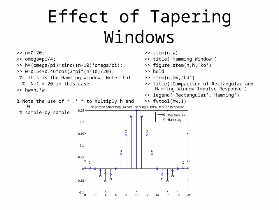
Effect of Tapering Windows>> n=0:20;>> omega=pi/4;>> h=(omega/pi)*sinc((n-10)*omega/pi);>> w=0.54+0.46*cos(2*pi*(n-10)/20); % This is the Hamming window. Note that % N-1 = 20 in this case>> hw=h.*w; % Note the use of “ .* “ to multiply h and w % sample-by-sample
>> stem(n,w)>> title('Hamming Window')>> figure,stem(n,h,'ko')>> hold>> stem(n,hw,'bd')>> title('Comparison of Rectangular and Hamming
Window Impulse Response')>> legend('Rectangular','Hamming')>> fvtool(hw,1)
0 2 4 6 8 10 12 14 16 18 20-0.1
-0.05
0
0.05
0.1
0.15
0.2
0.25Comparison of Rectangular and Hamming Window Impulse Response
Rectangular
Hamming
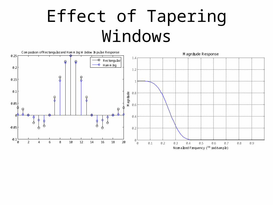
Effect of Tapering Windows
0 2 4 6 8 10 12 14 16 18 20-0.1
-0.05
0
0.05
0.1
0.15
0.2
0.25Comparison of Rectangular and Hamming Window Impulse Response
Rectangular
Hamming
0 0.1 0.2 0.3 0.4 0.5 0.6 0.7 0.8 0.90
0.2
0.4
0.6
0.8
1
1.2
1.4
Normalized Frequency ( rad/sample)
Mag
nitu
de
Magnitude Response
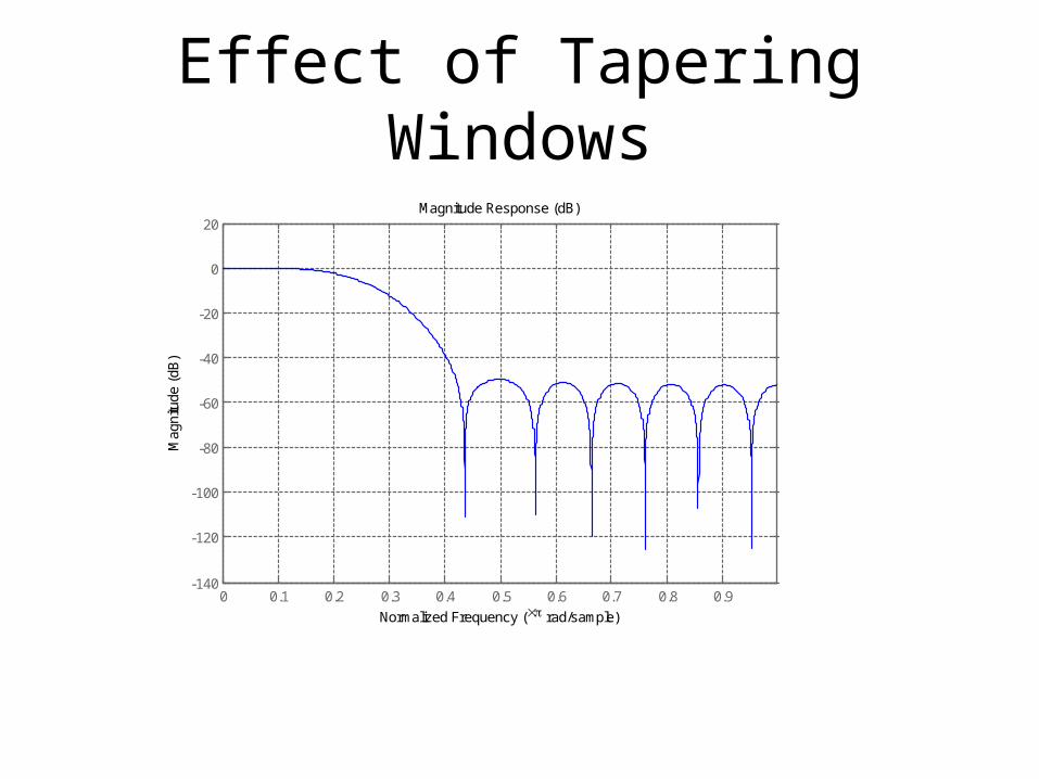
Effect of Tapering Windows
0 0.1 0.2 0.3 0.4 0.5 0.6 0.7 0.8 0.9-140
-120
-100
-80
-60
-40
-20
0
20
Normalized Frequency ( rad/sample)
Mag
nitu
de (
dB)
Magnitude Response (dB)
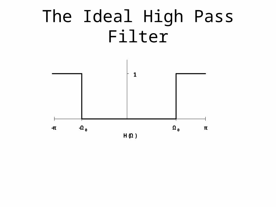
The Ideal High Pass Filter
-π π-Ω0 Ω0
1
H(Ω)

The Ideal High Pass Filter
0
0
0
0
0 0
0 0
1
21 1
2 21 1 1 1
2 2
1 1 1 1
2 2
1 1 1 1
2 2
π
π
π
π
π
π π
π π
[ ] ( ) π
π π
π π
π π
π π
j n
j n j n
j n j n
j n j n j n j n
j n j n j n j n
hn H e d
e d e d
e ejn jn
e e e en j n j
e e e en j n j
p
W
-
- WW W
- W
- WW W
- W
- W - W
W - W -
= W W
= W+ W
= +
é ù é ù= - + -ë û ë û
é ù é ù= - + + -ë û ë û
ò
ò ò
0
1 1 sin(π ) sin( )
π πn n
n n= - W
00[ ] sinc(π ) sinc( )
πh n n n n
W= - W - ¥ < <¥
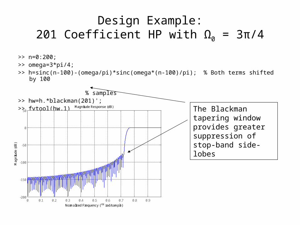
Design Example:201 Coefficient HP with Ω0 = 3π/4
>> n=0:200;>> omega=3*pi/4;>> h=sinc(n-100)-(omega/pi)*sinc(omega*(n-100)/pi); % Both terms shifted by 100 % samples>> hw=h.*blackman(201)';>> fvtool(hw,1)
0 0.1 0.2 0.3 0.4 0.5 0.6 0.7 0.8 0.9-200
-150
-100
-50
0
50
Normalized Frequency ( rad/sample)
Mag
nitu
de (
dB)
Magnitude Response (dB) The Blackman tapering window provides greater suppression of stop-band side-lobes
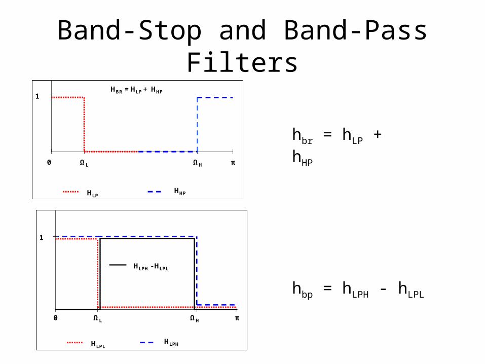
Band-Stop and Band-Pass Filters
0 πΩL ΩH
1HBR = HLP + HHP
HLPHHP
HLPLHLPH
ΩL ΩH π0
HLPH - HLPL
1
hbr = hLP + hHP
hbp = hLPH - hLPL
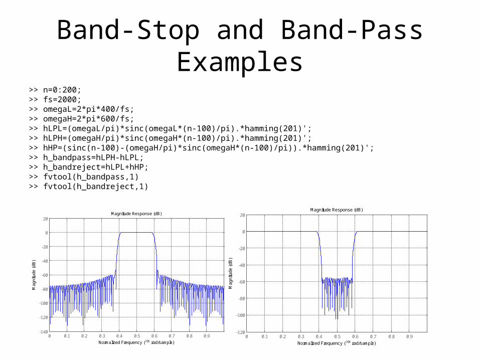
Band-Stop and Band-Pass Examples
>> n=0:200;>> fs=2000;>> omegaL=2*pi*400/fs;>> omegaH=2*pi*600/fs;>> hLPL=(omegaL/pi)*sinc(omegaL*(n-100)/pi).*hamming(201)';>> hLPH=(omegaH/pi)*sinc(omegaH*(n-100)/pi).*hamming(201)';>> hHP=(sinc(n-100)-(omegaH/pi)*sinc(omegaH*(n-100)/pi)).*hamming(201)';>> h_bandpass=hLPH-hLPL;>> h_bandreject=hLPL+hHP;>> fvtool(h_bandpass,1)>> fvtool(h_bandreject,1)
0 0.1 0.2 0.3 0.4 0.5 0.6 0.7 0.8 0.9-140
-120
-100
-80
-60
-40
-20
0
20
Normalized Frequency ( rad/sample)
Mag
nitu
de (
dB)
Magnitude Response (dB)
0 0.1 0.2 0.3 0.4 0.5 0.6 0.7 0.8 0.9-120
-100
-80
-60
-40
-20
0
20
Normalized Frequency ( rad/sample)
Mag
nitu
de (
dB)
Magnitude Response (dB)
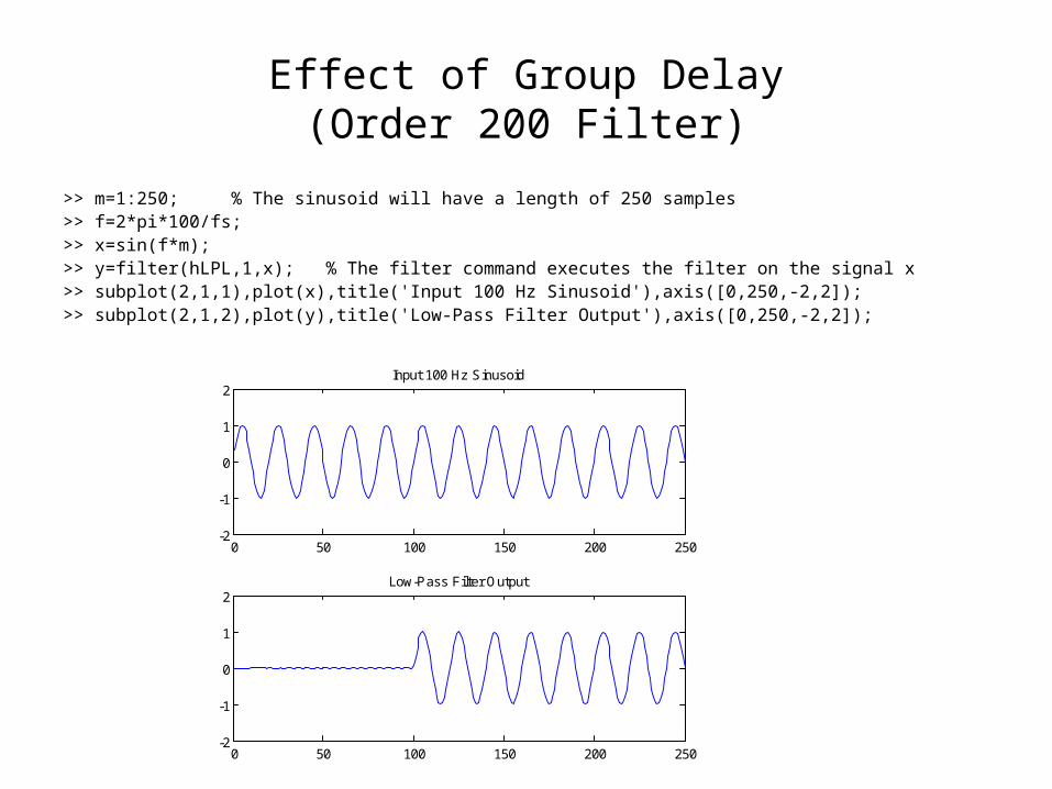
Effect of Group Delay(Order 200 Filter)
>> m=1:250; % The sinusoid will have a length of 250 samples>> f=2*pi*100/fs;>> x=sin(f*m);>> y=filter(hLPL,1,x); % The filter command executes the filter on the signal x>> subplot(2,1,1),plot(x),title('Input 100 Hz Sinusoid'),axis([0,250,-2,2]);>> subplot(2,1,2),plot(y),title('Low-Pass Filter Output'),axis([0,250,-2,2]);
0 50 100 150 200 250-2
-1
0
1
2Input 100 Hz Sinusoid
0 50 100 150 200 250-2
-1
0
1
2Low-Pass Filter Output
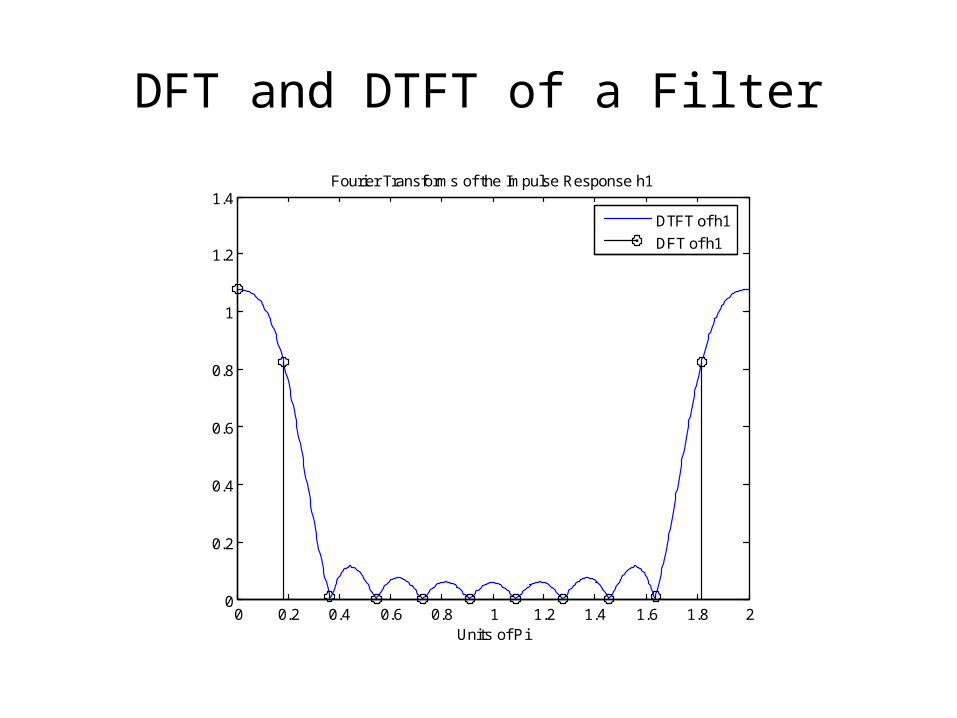
Sampling Method of FIR DesignBasic Theory
• The sampling method is based on the principle that the DFT is a sample of the DTFT
• To see this, take the DFT of the frequency response of a filter:
>> n=0:10; % Design a low pass filter by the window method>> omega=pi/4;>> h1=(omega/pi)*sinc(omega*(n-5)/pi);>> dtft_demo(h1,0,2*pi,512); % Display the DTFT of the filter>> hold>> [H1,f]=dft_demo(h1); % Take the DFT of the filter>> stem(f/pi,abs(H1),'k');>> legend('DTFT of h1','DFT of h1')>> title('Fourier Transforms of the Impulse Response h1')>> hold off
DFT and DTFT of a Filter
0 0.2 0.4 0.6 0.8 1 1.2 1.4 1.6 1.8 20
0.2
0.4
0.6
0.8
1
1.2
1.4Fourier Transforms of the Impulse Response h1
Units of Pi
DTFT of h1
DFT of h1
Sampling Method of FIR DesignBasic Theory
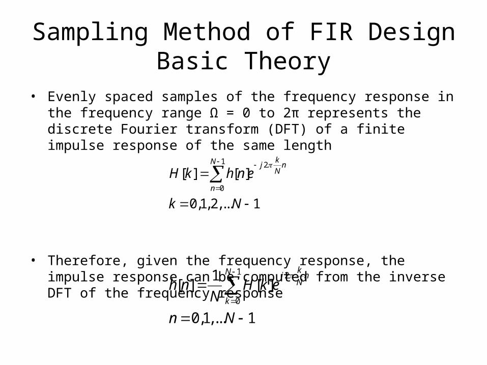
• Evenly spaced samples of the frequency response in the frequency range Ω = 0 to 2π represents the discrete Fourier transform (DFT) of a finite impulse response of the same length
• Therefore, given the frequency response, the impulse response can be computed from the inverse DFT of the frequency response
1 2
0
[ ] [ ]
0,1, 2,... 1
kN j nN
n
H k h n e
k N
1 2
0
1[ ] [ ]
0,1,... 1
kN j nN
k
h n H k eN
n N
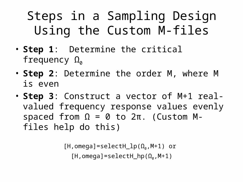
Steps in a Sampling DesignUsing the Custom M-files
• Step 1: Determine the critical frequency Ω0
• Step 2: Determine the order M, where M is even• Step 3: Construct a vector of M+1 real-valued
frequency response values evenly spaced from Ω = 0 to 2π. (Custom M-files help do this)
[H,omega]=selectH_lp(Ω0,M+1) or
[H,omega]=selectH_hp(Ω0,M+1)
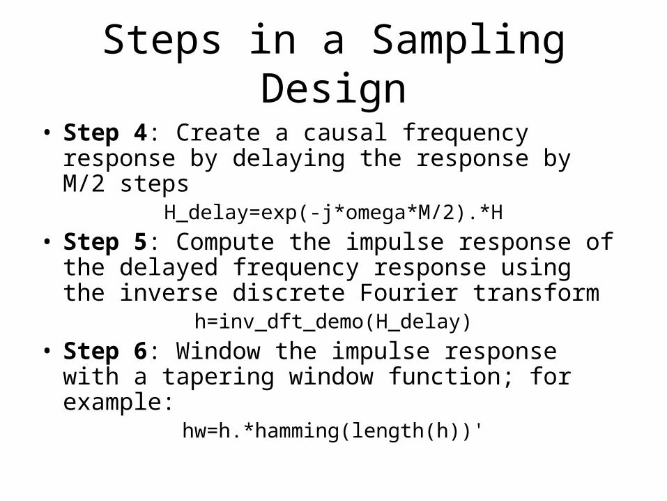
Steps in a Sampling Design
• Step 4: Create a causal frequency response by delaying the response by M/2 steps
H_delay=exp(-j*omega*M/2).*H
• Step 5: Compute the impulse response of the delayed frequency response using the inverse discrete Fourier transform
h=inv_dft_demo(H_delay)
• Step 6: Window the impulse response with a tapering window function; for example:
hw=h.*hamming(length(h))'
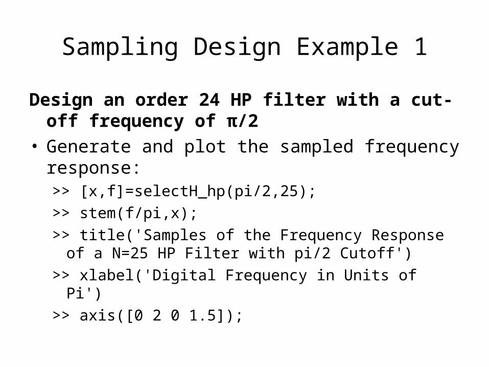
Sampling Design Example 1
Design an order 24 HP filter with a cut-off frequency of π/2
• Generate and plot the sampled frequency response:>> [x,f]=selectH_hp(pi/2,25);
>> stem(f/pi,x);
>> title('Samples of the Frequency Response of a N=25 HP Filter with pi/2 Cutoff')
>> xlabel('Digital Frequency in Units of Pi')
>> axis([0 2 0 1.5]);
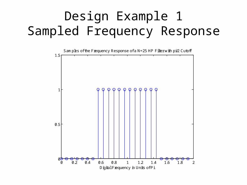
Design Example 1Sampled Frequency Response
0 0.2 0.4 0.6 0.8 1 1.2 1.4 1.6 1.8 20
0.5
1
1.5Samples of the Frequency Response of a N=25 HP Filter with pi/2 Cutoff
Digital Frequency in Units of Pi
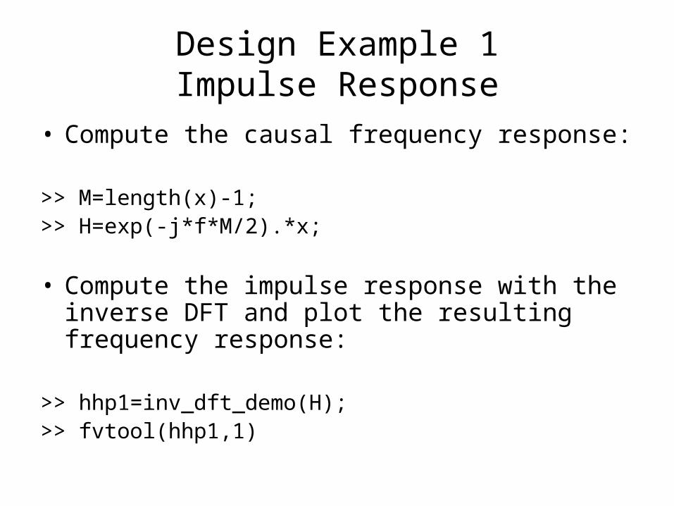
Design Example 1Impulse Response
• Compute the causal frequency response:
>> M=length(x)-1;>> H=exp(-j*f*M/2).*x;
• Compute the impulse response with the inverse DFT and plot the resulting frequency response:
>> hhp1=inv_dft_demo(H);>> fvtool(hhp1,1)
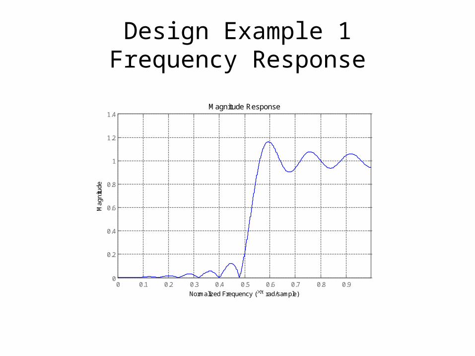
Design Example 1Frequency Response
0 0.1 0.2 0.3 0.4 0.5 0.6 0.7 0.8 0.90
0.2
0.4
0.6
0.8
1
1.2
1.4
Normalized Frequency ( rad/sample)
Mag
nitu
deMagnitude Response
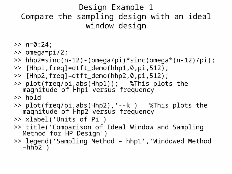
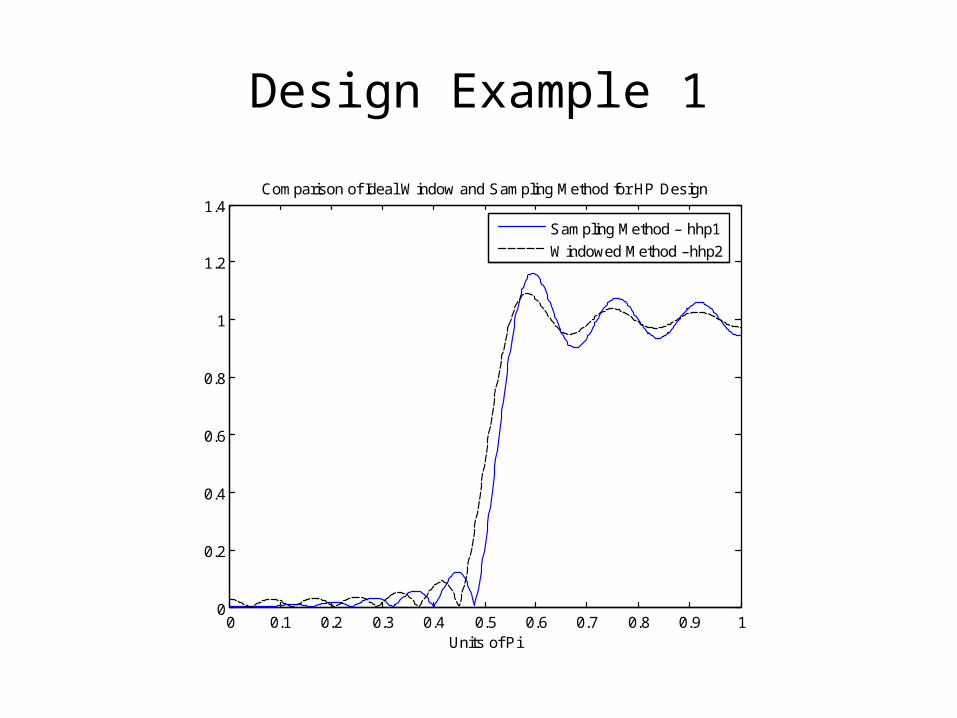
Design Example 1Compare the sampling design with an ideal window design
>> n=0:24;>> omega=pi/2;>> hhp2=sinc(n-12)-(omega/pi)*sinc(omega*(n-12)/pi);>> [Hhp1,freq]=dtft_demo(hhp1,0,pi,512);>> [Hhp2,freq]=dtft_demo(hhp2,0,pi,512);>> plot(freq/pi,abs(Hhp1)); %This plots the magnitude of Hhp1 versus
frequency>> hold>> plot(freq/pi,abs(Hhp2),'--k') %This plots the magnitude of Hhp2
versus frequency>> xlabel('Units of Pi')>> title('Comparison of Ideal Window and Sampling Method for HP
Design')>> legend('Sampling Method – hhp1','Windowed Method –hhp2')
Design Example 1
0 0.1 0.2 0.3 0.4 0.5 0.6 0.7 0.8 0.9 10
0.2
0.4
0.6
0.8
1
1.2
1.4
Units of Pi
Comparison of Ideal Window and Sampling Method for HP Design
Sampling Method – hhp1
Windowed Method –hhp2
Sampling Design 2
• Specifications:– low-pass filter of order 100, – a cut-off frequency 500 Hz – sampling frequency of 3000 Hz – Hamming window.
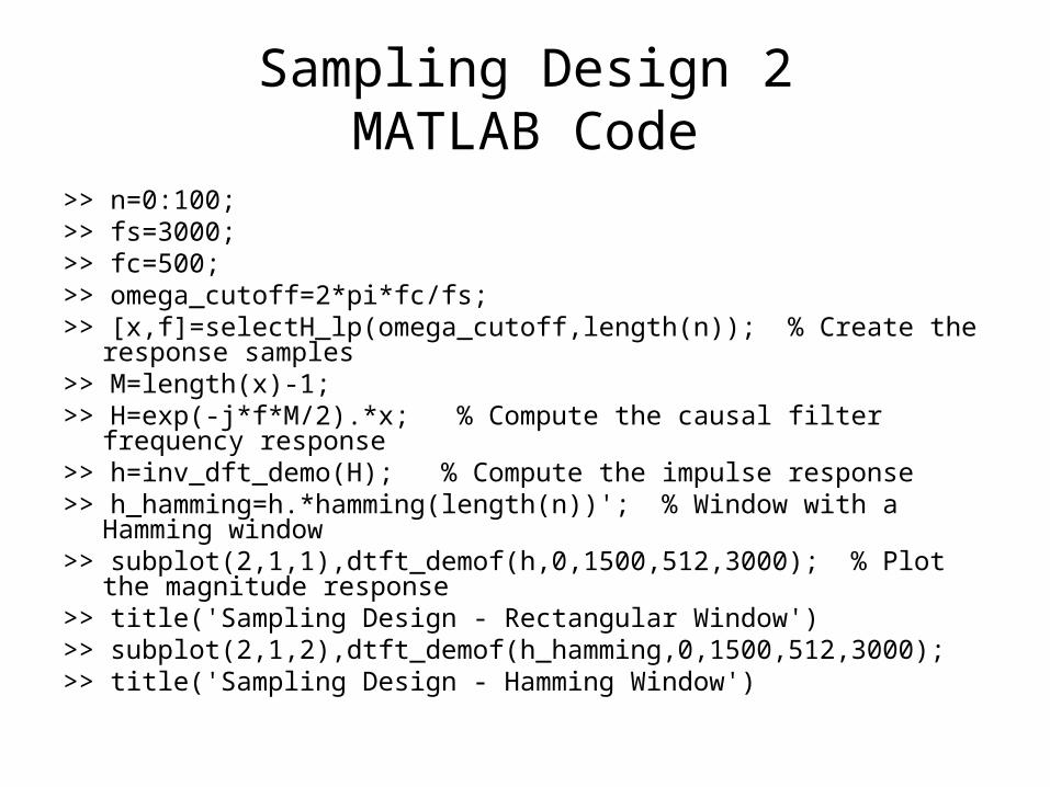
Sampling Design 2MATLAB Code
>> n=0:100;>> fs=3000;>> fc=500;>> omega_cutoff=2*pi*fc/fs;>> [x,f]=selectH_lp(omega_cutoff,length(n)); % Create the response samples>> M=length(x)-1;>> H=exp(-j*f*M/2).*x; % Compute the causal filter frequency response>> h=inv_dft_demo(H); % Compute the impulse response>> h_hamming=h.*hamming(length(n))'; % Window with a Hamming window>> subplot(2,1,1),dtft_demof(h,0,1500,512,3000); % Plot the magnitude
response>> title('Sampling Design - Rectangular Window')>> subplot(2,1,2),dtft_demof(h_hamming,0,1500,512,3000);>> title('Sampling Design - Hamming Window')
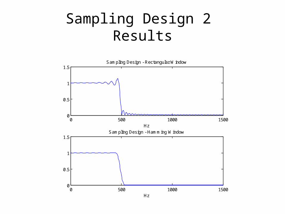
Sampling Design 2 Results
0 500 1000 15000
0.5
1
1.5Sampling Design - Rectangular Window
Hz
0 500 1000 15000
0.5
1
1.5Sampling Design - Hamming Window
Hz
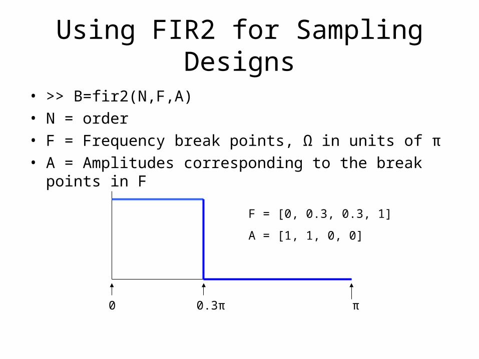
Using FIR2 for Sampling Designs
• >> B=fir2(N,F,A)• N = order• F = Frequency break points, Ω in units of π• A = Amplitudes corresponding to the break points in F
0 0.3π π
F = [0, 0.3, 0.3, 1]
A = [1, 1, 0, 0]
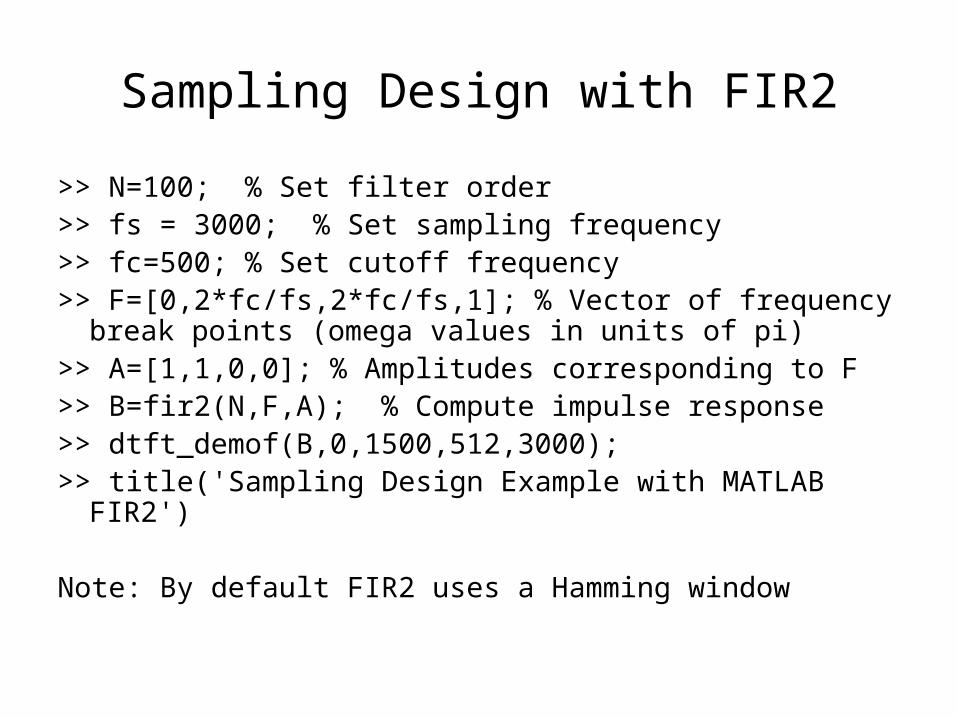
Sampling Design with FIR2
>> N=100; % Set filter order>> fs = 3000; % Set sampling frequency>> fc=500; % Set cutoff frequency>> F=[0,2*fc/fs,2*fc/fs,1]; % Vector of frequency break
points (omega values in units of pi)>> A=[1,1,0,0]; % Amplitudes corresponding to F>> B=fir2(N,F,A); % Compute impulse response>> dtft_demof(B,0,1500,512,3000);>> title('Sampling Design Example with MATLAB FIR2')
Note: By default FIR2 uses a Hamming window
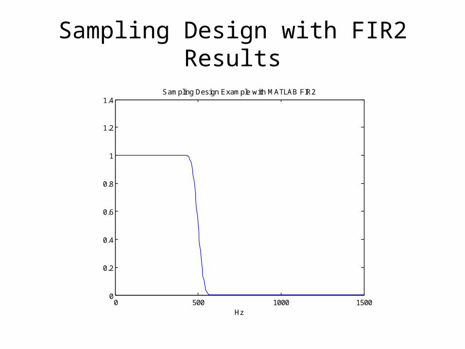
Sampling Design with FIR2Results
0 500 1000 15000
0.2
0.4
0.6
0.8
1
1.2
1.4Sampling Design Example with MATLAB FIR2
Hz
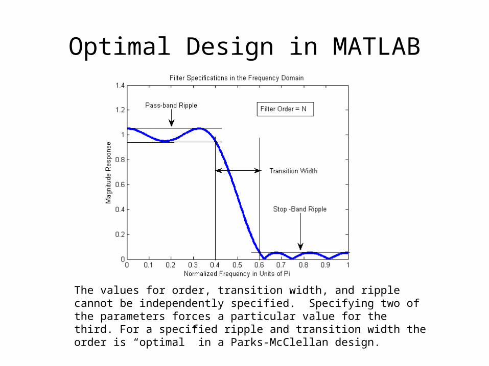
Optimal Design in MATLAB
The values for order, transition width, and ripple cannot be independently specified. Specifying two of the parameters forces a particular value for the third. For a specified ripple and transition width the order is “optimal” in a Parks-McClellan design.
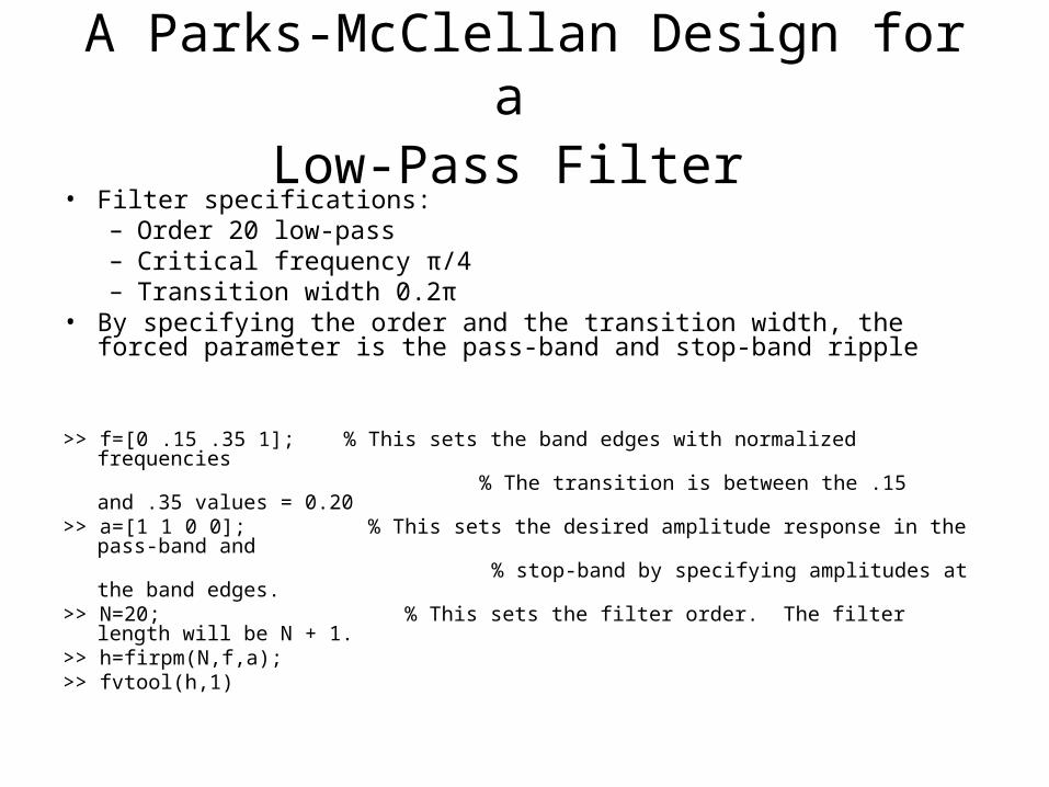
A Parks-McClellan Design for a Low-Pass Filter
• Filter specifications:– Order 20 low-pass– Critical frequency π/4– Transition width 0.2π
• By specifying the order and the transition width, the forced parameter is the pass-band and stop-band ripple
>> f=[0 .15 .35 1]; % This sets the band edges with normalized frequencies % The transition is between the .15 and .35 values = 0.20>> a=[1 1 0 0]; % This sets the desired amplitude response in the pass-band and % stop-band by specifying amplitudes at the band edges.>> N=20; % This sets the filter order. The filter length will be N + 1.>> h=firpm(N,f,a);>> fvtool(h,1)
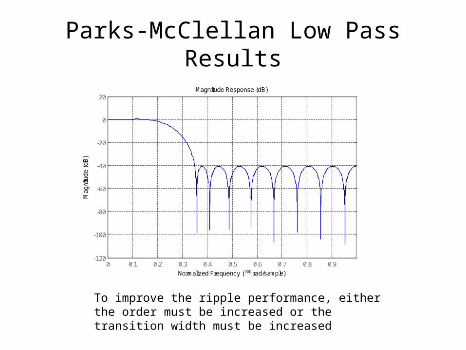
Parks-McClellan Low PassResults
0 0.1 0.2 0.3 0.4 0.5 0.6 0.7 0.8 0.9-120
-100
-80
-60
-40
-20
0
20
Normalized Frequency ( rad/sample)
Mag
nitu
de (
dB)
Magnitude Response (dB)
To improve the ripple performance, either the order must be increased or the transition width must be increased
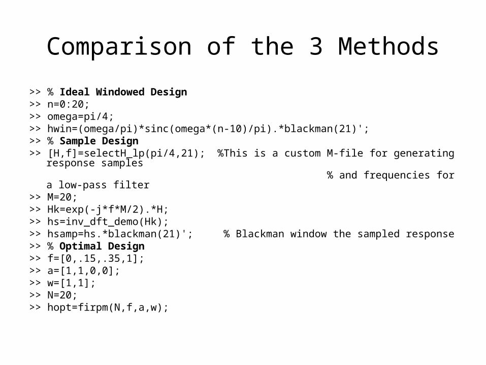
Comparison of the 3 Methods
>> % Ideal Windowed Design>> n=0:20;>> omega=pi/4;>> hwin=(omega/pi)*sinc(omega*(n-10)/pi).*blackman(21)';>> % Sample Design>> [H,f]=selectH_lp(pi/4,21); %This is a custom M-file for generating response samples % and frequencies for a low-pass filter>> M=20;>> Hk=exp(-j*f*M/2).*H;>> hs=inv_dft_demo(Hk);>> hsamp=hs.*blackman(21)'; % Blackman window the sampled response>> % Optimal Design>> f=[0,.15,.35,1];>> a=[1,1,0,0];>> w=[1,1];>> N=20;>> hopt=firpm(N,f,a,w);
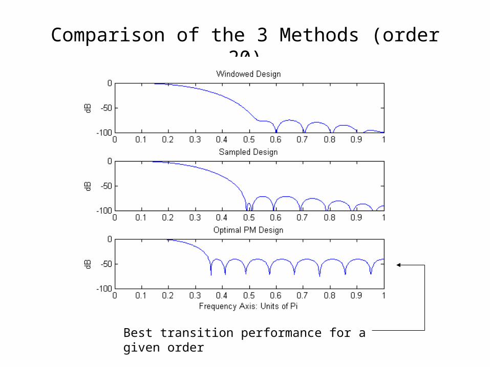
Comparison of the 3 Methods (order 20)
Best transition performance for a given order
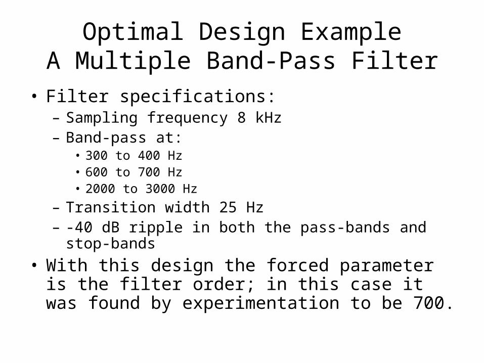
Optimal Design ExampleA Multiple Band-Pass Filter
• Filter specifications:– Sampling frequency 8 kHz– Band-pass at:
• 300 to 400 Hz• 600 to 700 Hz• 2000 to 3000 Hz
– Transition width 25 Hz– -40 dB ripple in both the pass-bands and stop-bands
• With this design the forced parameter is the filter order; in this case it was found by experimentation to be 700.
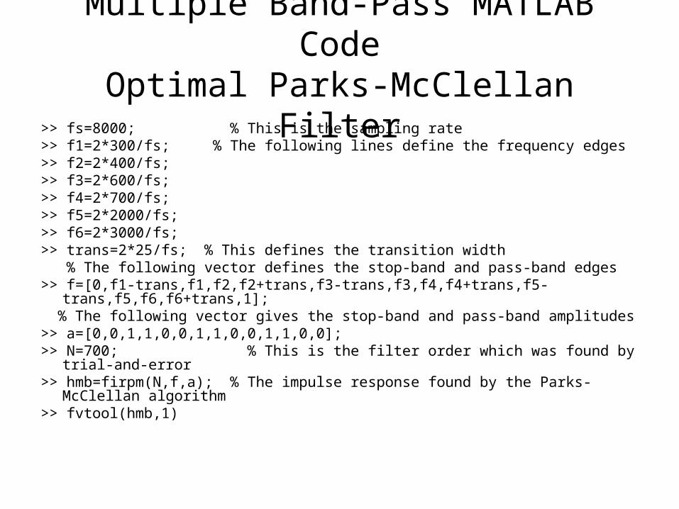
Multiple Band-Pass MATLAB CodeOptimal Parks-McClellan Filter
>> fs=8000; % This is the sampling rate>> f1=2*300/fs; % The following lines define the frequency edges>> f2=2*400/fs;>> f3=2*600/fs;>> f4=2*700/fs;>> f5=2*2000/fs;>> f6=2*3000/fs;>> trans=2*25/fs; % This defines the transition width % The following vector defines the stop-band and pass-band edges>> f=[0,f1-trans,f1,f2,f2+trans,f3-trans,f3,f4,f4+trans,f5-trans,f5,f6,f6+trans,1]; % The following vector gives the stop-band and pass-band amplitudes>> a=[0,0,1,1,0,0,1,1,0,0,1,1,0,0];>> N=700; % This is the filter order which was found by trial-and-error>> hmb=firpm(N,f,a); % The impulse response found by the Parks-McClellan
algorithm>> fvtool(hmb,1)
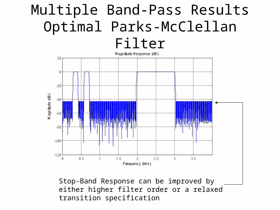
Multiple Band-Pass ResultsOptimal Parks-McClellan Filter
0 0.5 1 1.5 2 2.5 3 3.5-120
-100
-80
-60
-40
-20
0
20
Frequency (kHz)
Mag
nitu
de (
dB)Magnitude Response (dB)
Stop-Band Response can be improved by either higher filter order or a relaxed transition specification
Summary
• FIR filters allow the design of linear phase filters, which eliminate the possibility of signal phase distortion.
• Three methods of linear phase FIR design were discussed: – The ideal window method– The sampling method– The optimal Parks-McClellan method