kress smoothing transformation -...

KRESS SMOOTHING TRANSFORMATION FOR WEAKLY SINGULAR

FREDHOLM INTEGRAL EQUATION OF SECOND KIND

HASSAN MOHAMED SAEED BAWAZIR

UNIVERSITI TEKNOLOGI MALAYSIA

KRESS SMOOTHING TRANSFORMATION FOR WEAKLY SINGULAR

FREDHOLM INTEGRAL EQUATION OF SECOND KIND

HASSAN MOHAMED SAEED BAWAZIR

This dissertation is submitted

in partial fulfillment of the requirements for the

Master Degree of Science (Mathematics)

Faculty of Science

Universiti Teknologi Malaysia

MARCH 2006

iii

To

my beloved family and friends,

especially

my sons: Faisal and Mohamed.

iv

ACKNOWLEDGEMENT

In The Name Of ALLAH, The Most Beneficent, The Most Merciful

All praise is due only to ALLAH, the lord of the worlds. Ultimately, Only

ALLAH has given us the strength and courage to proceed with our entire life.

His works are truly splendid and wholesome, and his knowledge is truly complete

with due perfection.

I am particularly appreciative of my supervisor, Assoc. Prof. Dr. Ali

bin Abd Rahman for his invaluable supervision, guidance and assistance. He

has provided me with some precious ideas and suggestions throughout this

dissertation.

In addition I would like to thank Hadhramout University of Science &

Technology for their support. I am also grateful to Al-Sheikh Eng. Abdullah

Ahmad Bogshan for his financial support.

Also I would like to thank the Mathematics Department, Faculty of

Science, UTM, for providing the facilities.

I am grateful for the help of my best friends. Among these are Dr.

Mohammed M. S. Nasser and Mr. Omer Abdulaziz Mohamed Ali.

Besides, I want to dedicate heartiest gratitude to my beloved parents, my

uncle, and my wife for direct and indirect support and encouragement during the

completion of my dissertation.

v

ABSTRACT

This work investigates a numerical method for the second kind Fredholm

integral equation with weakly singular kernel k(x, y), in particular, when k(x, y) =

ln |x−y|, and k(x, y) = |x−y|−α, −1 ≤ x, y ≤ 1, 0 < α < 1. The solutions of such

equations may exhibit a singular behaviour in the neighbourhood of the endpoints

x = ±1. We introduce a new smoothing transformation based on the Kress

transformation for solving weakly singular Fredholm integral equations of the

second kind, and then using the Hermite smoothing transformation as a standard.

With the transformation an equation which is still weakly singular is obtained,

but whose solution is smoother. The transformed equation is then solved

numerically by product integration methods with interpolating polynomials. Two

types of interpolating polynomials, namely the Gauss-Legendre and Chebyshev

polynomials, have been used. Numerical examples are presented to investigate

the performance of the former.

vi

ABSTRAK

Kajian ini adalah untuk menyelidiki kaedah berangka bagi persamaan

kamiran Fredholm jenis kedua dengan inti aneh secara lemah k(x, y), khususnya,

apabila k(x, y) = ln |x − y|, dan k(x, y) = |x − y|−α, −1 ≤ x, y ≤ 1, 0 <

α < 1. Penyelesaian bagi persamaan ini mempamerkan perilaku singular dalam

kejiranan titik hujung x = ±1. Diperkenalkan juga penjelmaan berdasarkan

penjelmaan Kress untuk menyelesaikan kelemahan singular persamaan kamiran

Fredholm jenis kedua, seterusnya menggunakan penjelmaan Hermite, sebagai

piawai. Dengan penjelmaan ini persamaan yang masih lemah, diperolehi tetapi

penyelesaiannya lebih licin. Persamaan penjelmaan kemudian diselesaikan secara

berangka dengan kaedah hasildarab kamiran bersama polinomial interpolasi. Dua

jenis polinomial interpolasi, Gauss-Legendre dan Chebyshev, telah digunakan.

Contoh berangka diberikan menunjukkan keberkesanan kaedah ini.

vii

TABLE OF CONTENTS

CHAPTER TITLE PAGE

DISSERTATION STATUS DECLARATION

SUPERVISOR’S DECLARATION

TITLE PAGE i

DECLARATION ii

DEDICATION iii

ACKNOWLEDGEMENT iv

ABSTRACT v

ABSTRAK vi

TABLE OF CONTENTS vii

LIST OF TABLES xi

GLOSSARY xiv

LIST OF APPENDICES xv

1 PRELIMINARY REMARKS 1

1.1 Introduction 1

1.2 Problem Statement 4

1.3 Objectives of the Study 6

1.4 Scope of the Study 7

1.5 Simulation Tool 8

1.6 Dissertation’s Plan 9

viii

2 LITERATURE REVIEW 10

2.1 Introduction 10

2.2 Literature Review 11

2.3 Solution Behaviour 13

2.4 Hermite Transformation 14

2.5 Kress Transformation 16

3 PRODUCT INTEGRATION METHOD 20

3.1 Introduction 20

3.2 Integration Rules 21

3.3 Product Integration with Gaussian Abscissae

and Weights 24

3.3.1 Introduction 24

3.3.2 Application to Fredholm Equation

with Abel Kernels 25


with Logarithmic Kernels 27

3.4 Product Integration with Curtis-Clenshaw Points 28

3.4.1 Introduction 28





3.5 Concluding Remarks 33

4 QUADRATURE FORMULA 34

4.1 Introduction 34

4.2 An Integration Quadrature Formula 35

4.2.1 Hermite Smoothing Transformation 35

4.2.2 Kress Smoothing Transformation 37

ix

4.2.3 Modified Kress Transformation 41

4.3 Application to Weakly Singular Fredholm

Integral Equation of the Second Kind 43

4.3.1 Fredholm Weakly Singular Integral Equations

of the Second Kind with Abel Kernels 44

4.3.2 Fredholm Weakly Singular Integral Equations

of the Second Kind with Logarithmic Kernels 45

5 NUMERICAL RESULTS 47

5.1 Introduction 47

5.2 Product Integration with Gaussian Abscissae

and Weights 48

5.2.1 Weakly Singular Integral Equations


5.2.1.1 Matrix Elements 49

5.2.1.2 Examples 50




5.2.2.2 Examples 66

5.3 Product Integration with Curtis-Clenshaw Points 70




5.3.1.2 Examples 72




5.3.2.2 Examples 79

5.4 Discussion 88

6 SUMMARY AND CONCLUSIONS 91

x

6.1 Summary 91

6.2 Conclusions 92

6.3 Recommendations for Future Study 93

REFERENCES 94

APPENDICES

APPENDIX A 97

APPENDIX B 101

APPENDIX C 104

APPENDIX D 108

xi

LIST OF TABLES

TABLE NO. TITLE PAGE

3.1 Error Norm of Example 3.1 23

5.1 Error Norm of Example 5.1 with p = 2 58



5.4 The Values |θ256(t) − θn(t)| of Example 5.3 with p = 2 59



5.7 The Values |θ256(t) − θn(t)| of Example 5.4 60

5.8 The Values |θ256(t) − θn(t)| of Example 5.5 with

α0 = α2 = 4, α1 = 9 60


α0 = α1 = 3 60







α0 = α2 = 4, α1 = 9 62


α0 = α1 = 3 63





xii

5.21 Error Norm of Example 5.11. 68

5.22 The values |θ256(t) − θn(t)| of Example 5.12 68

5.23 The values |θ128(t) − θn(t)| of Example 5.13 with

α0 = α1 = 2 68

5.24 The values |θ128(t) − θn(t)| of Example 5.13 with

α0 = α1 = 3 69

5.25 The values |θ128(t) − θn(t)| of Example 5.14 with p = 2 69

5.26 The values |θ128(t) − θn(t)| of Example 5.14 with p = 3 70



5.29 Error Norm of Example 5.15 with α0 = α1 = 2 74









α0 = α1 = 3 76


α0 = α2 = 4, α1 = 9 77












xiii

α0 = α1 = 3 87


α0 = α2 = 4, α1 = 9 87

xiv

GLOSSARY

GM Gauss method

CM Clenshaw method

HT Hermite transformation

KT Kress transformation

MKT Modified Kress transformation

xv

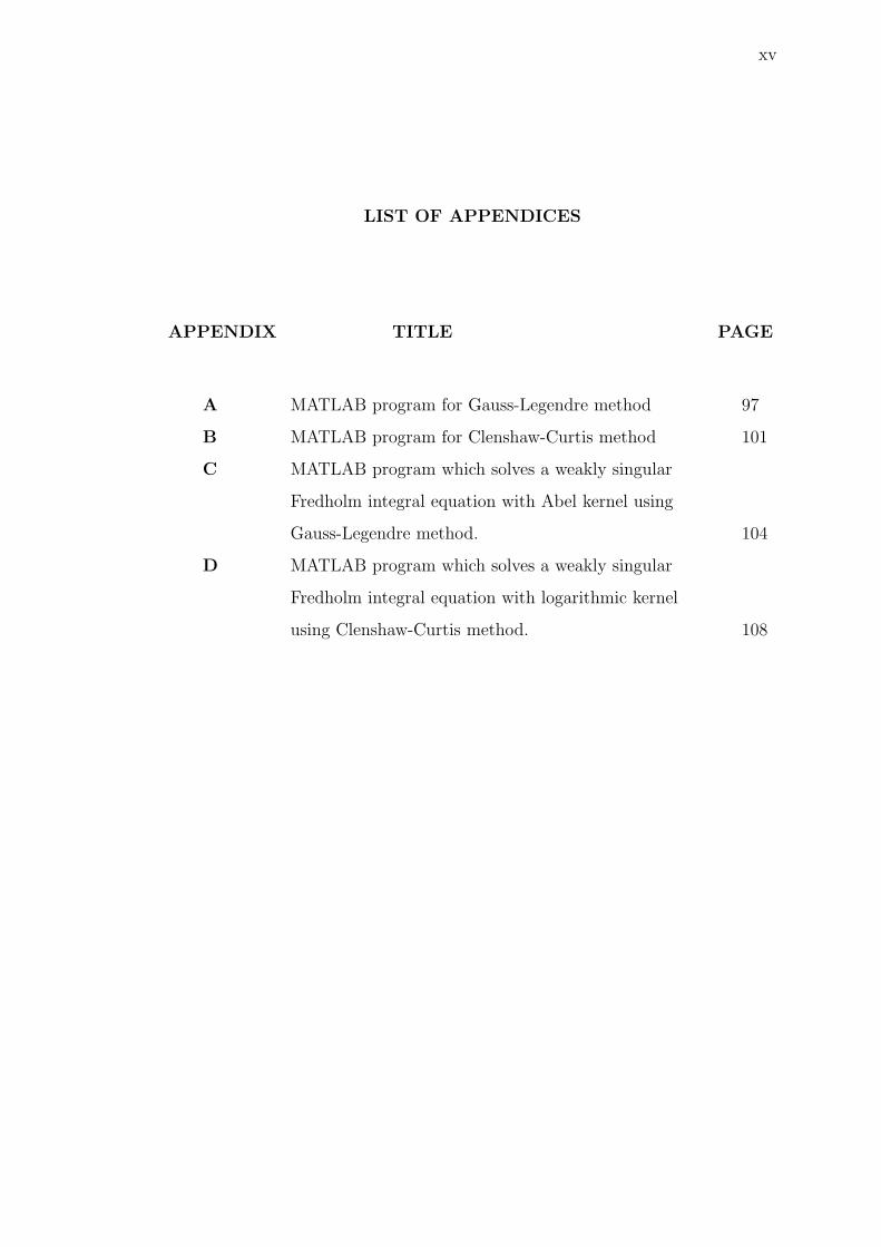
LIST OF APPENDICES

APPENDIX TITLE PAGE

A MATLAB program for Gauss-Legendre method 97

B MATLAB program for Clenshaw-Curtis method 101

C MATLAB program which solves a weakly singular

Fredholm integral equation with Abel kernel using

Gauss-Legendre method. 104

D MATLAB program which solves a weakly singular

Fredholm integral equation with logarithmic kernel

using Clenshaw-Curtis method. 108

CHAPTER 1

PRELIMINARY REMARKS

1.1 Introduction

An integral equation is an equation in which the unknown function f(x)

to be determined appears under the integral sign. A typical form of an integral

equation in f(x) is of the form

f(x) − λ

∫ β(x)

α(x)

k(x, y)f(y)dy = g(x), (1.1)

where k(x, y) is called the kernel of the integral equation, and α(x) and β(x) are

the limits of integration. It is important to point out that the kernel k(x, y) and

the function g(x) in (1.1) are given in advance, g(x) is called input function.

The standard form of a Volterra linear integral equation, where the limits

of integration are functions of rather than constants, are of the form

φ(x)f(x) − λ

∫ x

a

k(x, y)f(y)dy = g(x), a ≤ x ≤ b, (1.2)

and the standard form of a Fredholm linear integral equation, where the limits

of integration α(x) and β(x) are constants (say a and b), is given by the form

φ(x)f(x) − λ

∫ b

a

k(x, y)f(y)dy = g(x), a ≤ x, y ≤ b, (1.3)

2

where the kernel of the integral equation, k(x, y), and the function g(x) are given

in advance, and λ is a parameter. The equations (1.2) and (1.3) is called linear

because the unknown function f(x) under the integral sign occurs linearly, i.e,

the power of f(x) is one.

The value of φ(x) will give rise to the following kinds of Fredholm linear

integral equations:

1. When φ(x) = 0, equation (1.3) becomes

g(x) + λ

∫ b

a

k(x, y)f(y)dy = 0, a ≤ x, y ≤ b, (1.4)

and is called Fredholm integral equation of the first kind.

2. When φ(x) = 1, equation (1.3) becomes

f(x) − λ

∫ b

a

k(x, y)f(y)dy = g(x), a ≤ x, y ≤ b, (1.5)

and is called linear Fredholm integral equation of the second kind. In fact, the

form of equation (1.5) can be obtained from (1.3) by dividing both sides of (1.3)

by φ(x), provided that φ(x) �= 0,

As a special case of equation (1.5) when g(x) = 0, we have the equation

f(x) − λ

∫ b

a

k(x, y)f(y)dy = 0, a ≤ x, y ≤ b, (1.6)

By a boundary value problem for an ordinary differential equation of nth

order, we mean the problem of determining the solution of the equation in a

certain interval, on the boundaries of which the solution and its derivatives of

order not higher than n − 1 take on prescribed values, or satisfy given relations.

These problems lead to Fredholm integral equations (see Pogorzelski (1966),

p.221).

The boundary value problems for partial differential equations the

parabolic and hyperbolic type lead to Volterra integral equations, while the

3

boundary value problems for partial differential equations of the elliptic type

yield Fredholm equations.

The solution of the Dirichlet and von Neumann problems are one of

applications of the theory of Fredholm equation (see Pogorzelski (1966), p.230).

Equation (1.1) is called singular if the lower limit, the upper limit or both

limits of integration are infinite. In addition, the equation (1.1) is also called a

singular integral equation if the kernel k(x, y) becomes infinite at one or more

points in the domain of integration (see Wazwaz (1997), p.7).

The kernels which become unbounded at x = y, for example

k(x, y) = |x − y|−α, 0 < α < 1,

or

k(x, y) = ln |x − y|,

are said to have a weak singularties (see Baker (1977), p.68). The case where

k(x, y) and g(x) are piecewise-continuous, with finite jump discontinuities only

on lines parallel to the coordinate axes; these ‘singularities’ are called ‘mild’ (see

Baker (1977), p.526).

Supposing that our functions k(x, y) and g(x) are piecewise-continuous

and bounded, then in solving (1.6) we seek values of the parameter λ for which

(1.6) has a non-trivial solution f(x). Such a value λ is called a characteristic

value and the solution is called the eigenfunction (see Baker (1977), p. 4).

In general we cannot guarantee the existence of any solution λ �= 0 for

equation (1.6). In particular if the kernel k(x, y) is not identically zero, real, and

k(x, y) = k(y, x) ( in this case k(x, y) is said to be real and symmetric), there is

at least one non-zero characteristic value and all of the characteristic values are

real.

4

A value λ such that the equation (1.5) is uniquely solvable (when g(x)

is piecewise-continuous but otherwise arbitrary) is known as a regular value. If

λ is a characteristic value and ψ(x) a corresponding eigenfunction then to any

solution f(x) of equation (1.5) there corresponds another solution f(x) + αψ(x),

where α is arbitrary. Thus if λ is a characteristic value it cannot be a regular

value. Moreover, if λ is not a characteristic value it can be shown that equation

(1.5) has a unique solution, for arbitrary g(x), and hence that λ is a regular value

(see Baker (1977), p. 15).

The previous results, which are about uniqueness and existence of the

solution of Fredholm integral equations of the first and second kinds, are obtained

under the supposition that the kernel k(x, y) and the input function g(x) are

piecewise-continuous and bounded. Additional consideration of weakly singular

Fredholm integral equation requires some concepts such as compact integral

operators, and Banach spaces; furthermore it requires some theorems like the

Fredholm Alternative. Consider a weakly singular Fredholm integral equation of

the second kind of the form

f(x) − λ

∫ 1

−1

k(x, y)f(y)dy = g(x) − 1 ≤ x, y ≤ 1, (1.7)

with

k(x, y) = |x − y|−α, 0 < α < 1,

or

k(x, y) = ln |x − y|.

It can be proved that (1.7) has a unique solution if and only if the corresponding

homogeneous equation has only the trivial solution; for more details see Atkinson

(1997), pages 6-13.

1.2 Problem Statement

This dissertation introduces a new smoothing transformation based on

the Kress transformation for solving weakly singular Fredholm integral equations

5

of the second kind, and then using the Hermite smoothing transformation as a

standard, investigates the performance of the former.

Consider weakly singular Fredholm integral equation of second kind of the

form

f(x) − λ

∫ 1

−1

k(x, y)f(y)dy = g(x) − 1 ≤ x, y ≤ 1, (1.8)

with weakly singular kernels of one of the following forms:

Abel kernel

k(x, y) = |x − y|−α, 0 < α < 1,

logarithmic kernel

k(x, y) = ln |x − y|,

where −1 ≤ x ≤ 1.

The numerical solution of (1.8) is closely related to the solution of a linear

algebraic system. Indeed, the main goal of the numerical methods to solve (1.8) is

to reduce it approximately to a linear algebraic system. Then the linear algebraic

system is solved to obtain an approximate solution of (1.8) as shown in the next

chapters.

The numerical treatment of weakly singular integral equations should take

into account the nature of the singularities at the endpoints x = ±1. Some of the

techniques that can be used to solve these integral equations are as follows:

1. Canceling the singularity (of the kernel).

2. Modified quadrature method.

3. Smoothing the kernel.

4. Approximating the kernel by a degenerate kernel.

5. Expansion methods (Galerkin and collocation methods).

6. Product integration.

6

Kress (1990) introduces an algebraic transformation for smoothing the

solution of a boundary Fredholm integral equation in domains with corners.

The solution of this integral equation has a singularity at the corner point. He

considers integral equations of the second kind in the slightly unconventional

form, and supposes that the input function is continuous, so we will focus on

using of his transformation when the input function g(x) is smooth. We will do

some modifications of the Kress transformation to be applicable with non-smooth

input functions. More details for these transformations will be given later.

Elliott and Prossdorf (1995) introduce a transformation of [0,1] onto itself

such that an arbitrary number of derivatives vanish at the end points 0 and 1. If

the transformed kernel is dominated near the origin by a Mellin kernel then they

give conditions under which the use of a modified Euler-Maclaurin quadrature

rule and the Nystrom method gives an approximate solution which converges to

the exact solution of the original equation.

Monegato and Scuderi (1998) introduce a simple smoothing change

of variable to solve one-dimensional linear weakly singular integral equations

on bounded intervals, with input functions which may be smooth or not.

In both cases either the input function is smooth or non-smooth, they

define the smoothing transformation w = w(t) by using piecewise Hermite

interpolation polynomial HM(t), so we will call this transformation as the Hermite

transformation. We will focus on using the Hermite smoothing transformation

for both cases as a standard. We will give more details for this transformation

later.

1.3 Objectives of the Study

1. Using the Hermite smoothing transformation, reduce a second kind

Fredholm integral equation with a weakly singular kernel, for both smooth

7

and non-smooth input functions, to an equivalent equation with smoother

solution.

2. Using the Kress smoothing transformation, reduce a second kind Fredholm

integral equations with a weakly singular kernel, for smooth input functions,

to an equivalent equation with smoother solution.

3. Introduce a new transformation by modifying the Kress transformation so

that it can be applied to non-smooth input functions.

4. Using the modified Kress transformation, reduce a second kind Fredholm

integral equation with a weakly singular kernel, for non-smooth input

functions, to an equivalent equation with smoother solution.

5. Solve the new transformed equation using the product integration method.

6. Compare the numerical results from the transformations.

1.4 Scope of the Study

This dissertation focuses on introducing a new usage of the Kress

smoothing transformation for solving weakly singular Fredholm integral equation

of second kind, and then using the Hermite smoothing transformation as a

standard, investigates the performance of the former.

Firstly, we shall introduce a quadrature formula for the numerical

evaluation of integrals of the form

∫ 1

−1

f(x)dx, (1.9)

where the integrand is continuous on the interval (-1,1) and has singularities at

the endpoints ±1. The idea of the new quadrature formula is to use the Hermite

and Kress smoothing transformations to reduce the integral (1.9) to an equivalent

integral with a smooth integrand.

8

Next, each transformation will be used to reduce, respectively, a second

kind Fredholm integral equation with a weakly singular kernel to an equivalent

equation with smoother solution.

The new transformed equation will be discretized using the product

integration method to obtain an equivalent linear algebraic system. The following

product integration methods will be used:

1. Product integration with Gauss-Legendre points and weights.

2. Product integration with Clenshaw-Curtis (practical Chebyshev) points.

The linear system will be solved using the MATLAB software (refer to

Rosenberg (2001)) to obtain an approximate solution to the integral equation.

1.5 Simulation Tool

MATLAB is a language for mathematical computations whose

fundamental data types are vectors and matrices. It is distinguished from

languages such as FORTRAN and C/C++ by operating at a higher mathematical

level, including hundreds of operations such as matrix inversion, the singular value

decomposition, and the fast Fourier transform as built-in commands. It is also

a problem-solving environment, processing top-level commends by an interpreter

rather than a compiler and providing in-line access to 2D and 3D graphics.

The version of MATLAB, MATLAB7.0, is used in the present study, and

the programs are written to reduce an integral equation to a linear algebraic

system, and to calculate the numerical solution of the algebraic problem. The

calculations are done on Intel Pentium 4 2.4GHz Personal Computer.

9

1.6 Dissertation’s Plan

This dissertation contains six chapters.

Chapter 2 is a literature review of some important numerical methods, the

solution behaviour, the Hermite smoothing transformation and Kress smoothing

transformation. Chapter 3 contains a discussion of the product integration

method with Gaussian abscissae and product integration method with Curtis-

Clenshaw points, and the application of the two methods to solving weakly

singular Fredholm integral equations of the second kind with Abel and logarithmic

kernels. Chapter 4 discusses the quadrature formula to obtain a numerical

approximation of integrals with singularities at the endpoints of the interval of

the integration by using the smoothing transformations. Chapter 5 presents the

numerical results of this study. Finally, a conclusion of the work is given in

Chapter 6.

94

REFERENCES

Atkinson, Kendall E. (1967). The Numerical Solution of Fredholm Integral

Equation of Second Kind SIAM J. Numer. Anal. 4: 337–348.

Atkinson, Kendall E. (1976). A Survey of Numerical Methods for Solution of

Fredholm Integral Equation of Second Kind. SIAM, Philadelphia.

Atkinson, Kendall E. (1997). The Numerical Solution of Integral Equation of the

Second Kind. Cambridge University press.

Baker, C.T.H. (1977). The Numerical Treatment of Integral Equation. Oxford

University Press.

Clenshaw, C. W. and Curtis, A.R. (1960). A Method for Numerical Integration

on an Automatic Computer. Numer. Math. 2: 197–205.

Criscuolo, G., Mastroianni, G. and Monegato, G. (1990). Convergence Properties

of A class of Product Formulas for Weakly Singular Integral Equations. Math.

Comp. 55: 213–230.

Davis, Philip F. and Rabinowitz, Philip. (1984). Methods of Numerical

Integration. 2nd ed. Academic Press Inc.

Delves, L.M. and Mohamed, J. L. (1985). Computational Methods for Integral

Equations. Cambridge University Press, Cambridge.

Elliott, David and Prossdorf, Siegfried. (1995). An algorithm for the approximate

95

solution of integral equations of Mellin type. Numer. Math. 70: 427–452.

Graham , Ivan G. (1982). Singularity expansions for the solutions of second kind

Fredholm integral equations with weakly singular convolution kernels. J.

Integral Equations 4: 1–30.

Graham, Ivan G. (1982). Galerkin Method for Second Kind Integral Equations

with Singularities. Math. Comp. 39: 519–533.

Graham, I. and Chandler, G. (1988). High order methods for linear functionals

of solutions of second kind integral equations. SIAM J. Numer. Anal. 25:

1118–1137.

Jerri, Abdul J. (1985). Introduction to Integral Equations with Applications.

Marcel Dekker, INC. New York.

Kaneko, Hideaki and Xu, Yuesheng. (1991). Numerical Solutions for Weakly

Singular Fredholm Integral Equations of the Second Kind. Appl. Numer.

Math. 7: 167–177.

Kaneko, Hideaki and Xu, Yuesheng. (1994). Numerical Gauss-Type Quadratures

for Weakly Singular Integrals and Their Application to Fredholm Integral

Equations of the Second Kind. Math. Comp. 62: 739-753.

Kress, Rainer. (1989). Linear Integral Equations. Berlin: Springer-Verlag.

Kress, Rainer. (1990). A Nystrom method for boundary integral equations in

domains with corners. Numer. Math. 58:145–161.

Kythe, Prem K. and Puri, Pratap. (2002). Computational Methods for Linear

Integral Equations. Birkhauser Boston.

Linz, Peter. (1985). Analytical and Numerical Methods for Volterra Equations.

SIAM Pub., Philadelphia.

96

Monegato, G. and Scuderi, L. (1998). High Order Methods for Weakly Singular

Integral Equations with Non Smooth Input Function. Math. Comp. 67:

1493–1515.

Piessens, Robert and Branders, Maria. (1976). Numerical Solution of Integral

Equations of Mathematical Physics Using Chebyshev Polynomials. J. Comp.

Phys. 21: 178–196.

Pogorzelski, W. (1966). Integral Equation and Their Applications. Vol. 1. Oxford:

Pergamon Press.

Rosenberg, Jonathan M. (2001). A Guide to Matlab: For Beginners and

Experienced Users. Cambridge University Press.

Schneider, Claus. (1981). Product Integration for Weakly Singular Integral

Equations. Math. Comp. 36: 207–213.

Sloan, Ian H. (1980). On Choosing the Points in Product Integration. J. Math.

Phys. 21: 1032-1039.

Wazwaz, Abdul-Majid. (1997). A first course in integral equations. World

Scientific.

Young, A. (1954). Approximate Product-Integration. Proc. Roy. Soc. London

Ser. A 224: 552–561.

APPENDICES

APPENDIX A

MATLAB program to find the approximation

matrix using Gauss-Legendre method.

% gau_point.m

function [t,wg] = gau_point(n)

n1=n+1; e1=n1*(n1+1);

if mod(n1,2)==0

m=n1/2

else

m=(n1+1)/2

end

for i=1:m

t=(4*i-1)*pi/(4*n1+2); xo=(1-(1-1/n1)/(8*n1^2))*cos(t);

pkm1=1; pk=xo;

for k=2:n1

t1=xo*pk; pkp1=t1-pkm1-(t1-pkm1)/k+t1;

pkm1=pk; pk=pkp1;

end

den=1-xo^2; d1=n1*(pkm1-xo*pk);

dpn=d1/den; dpn2=(2*xo*dpn-e1*pk)/den;

dpn3=(4*xo*dpn2+(2-e1)*dpn)/den;

dpn4=(6*xo*dpn3+(6-e1)*dpn2)/den;

u=pk/dpn; v=dpn2/dpn;

h=-u*(1+0.5*u*(v+u*(v^2-dpn3/(3*dpn))));

p=pk+h*(dpn+0.5*h*(dpn2+h/3*(dpn3+0.25*h*dpn4)));

dp=dpn+h*(dpn2+0.5*h*(dpn3+h*dpn4/3));

98

h=h-p/dp; x(i)=xo+h;

fx=d1-h*e1*(pk+0.5*h*(dpn+h/3*(dpn2+0.25*h*(dpn3+0.2*h*dpn4))));

w(i)=2*(1-x(i)^2)/(fx^2);

end

if (m+m > n1 )

x(m)=0;

end

if (m+m > n1 )

t(m)=0;

wg(m)=w(m);

for i=0:m-2

t(i+1)=-x(i+1); t(i+m+1)=x(m-i-1);

wg(i+1)=w(i+1); wg(i+m+1)=w(m-i-1);

end

else

for i=0:m-1

t(i+1)=-x(i+1); t(i+m+1)=x(m-i);

wg(i+1)=w(i+1); wg(i+m+1)=w(m-i);

end

end

1. For kernel k(x, y) = |x − y|− 12

% Gau_Leg_Abs_Mat.m

function [w, p] = Gau_Leg_Abs_Mat(n)

[t,wg] = gau_point(n);

for j=0:n

p(1,j+1)=1;

p(2,j+1)=t(j+1);

end

for i=1:n-1

for j=0:n

p(i+2,j+1)=((2*i+1)*t(j+1)*p(i+1,j+1)-i*p(i,j+1))/(i+1);

end

end

for i=0:n

a(1,i+1)=2*(sqrt(1+t(i+1))+sqrt(1-t(i+1)));

end

for i=0:n

a(2,i+1)=t(i+1)*a(1,i+1)+2*((1-t(i+1))^1.5-(1+t(i+1))^1.5)/3;

end

99

for k=1:n-1

for i=0:n

a(k+2,i+1)=2*((2*k+1)*t(i+1)*a(k+1,i+1)-0.5*(2*k-1)*a(k,i+1))/...(2*k+3);

end

end

for i=0:n

for j=0:n

sum1=0;

for k=0:n

sum1=sum1+(2*k+1)*p(k+1,j+1)*a(k+1,i+1)/2;

end

w(i+1,j+1)=wg(j+1)*sum1;

end

end

2. For kernel k(x, y) = ln |x − y|

% Gau_Leg_log_Mat.m

function [w,p] = Gau_Leg_Log_Mat(n)

[t,wg] = gau_point(n);

for j=0:n

p(1,j+1)=1;

p(2,j+1)=t(j+1);

end

for i=1:n-1

for j=0:n

p(i+2,j+1)=((2*i+1)*t(j+1)*p(i+1,j+1)-i*p(i,j+1))/(i+1);

end

end

for i=0:n

a(1,i+1)=(1+t(i+1))*log(1+t(i+1))+(1-t(i+1))*log(1-t(i+1))-2;

end

for i=0:n

a(2,i+1)=0.5*(1-t(i+1)^2)*log((1-t(i+1))/(1+t(i+1)))-t(i+1);

end

for i=0:n

a(3,i+1)=0.5*t(i+1)*(1-t(i+1)^2)*log((1-t(i+1))/(1+t(i+1)))...+(2-3*t(i+1)^2)/3;

end

for k=2:n-1

100

for i=0:n

a(k+2,i+1)=((2*k+1)*t(i+1)*a(k+1,i+1)-(k-1)*a(k,i+1))/(k+2);

end

end

for i=0:n

for j=0:n

sum1=0;

for k=0:n

sum1=sum1+(2*k+1)*p(k+1,j+1)*a(k+1,i+1)/2;

end

w(i+1,j+1)=wg(j+1)*sum1;

end

end

101

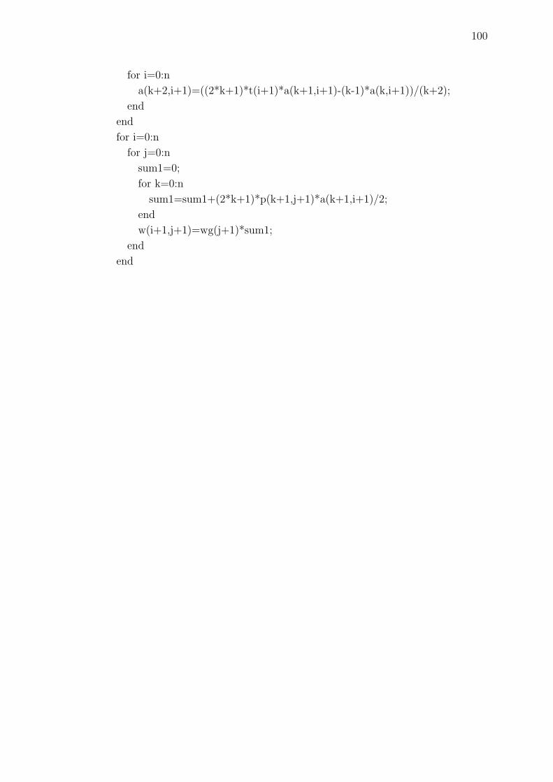
APPENDIX B

MATLAB program to find the approximation

matrix using Clenshaw-Curtis method

1. For kernel k(x, y) = |x − y|− 12

% Cel_Cur_Abs_Mat.m

function [w,t] = Cel_Cur_Abs_Mat(m)

for i=0:m

t(i+1)=cos(i*pi/m);

end

for i=0:m

a(1,i+1)=2*(sqrt(1+t(i+1))+sqrt(1-t(i+1)));

end

for i=0:m

a(2,i+1)=t(i+1)*a(1,i+1)+2*((1-t(i+1))^1.5-(1+t(i+1))^1.5)/3;

end

for i=0:m

a(3,i+1)=4*t(i+1)*a(2,i+1)-(2*(t(i+1))^2 +1)*a(1,i+1)...+4*((1-t(i+1))^(2.5)+(1+t(i+1))^(2.5))/5;

end

for j=2:m-1

for i=0:m

a(j+2,i+1)=(2*j+2)*(2*t(i+1)*a(j+1,i+1)-(2*j-3)*a(j,i+1)/(2*(j-1))...+2*(sqrt(1-t(i+1))-((-1)^j)*sqrt(1+t(i+1)))/(1-j^2))/(2*j+3);

end

end

p(1)=0.5; p(m+1)=0.5;

for i=1:m-1

p(i+1)=1;

end

for j=0:m

for i=0:m

sum=(a(1,i+1)+a(m+1,i+1)*cos(j*pi))/2;

for k=1:m-1

sum=sum+a(k+1,i+1)*cos(j*k*pi/m);

end

102

w(i+1,j+1)=2*p(j+1)*sum/m;

end

end

2. For kernel k(x, y) = ln |x − y|

% Cel_Cur_log_Mat.m

function [w,t] = Cel_Cur_Log_Mat(n)

for i=0:n

t(i+1)=cos((i*pi)/n);

end

a(1,1) =2*log(2)-2; a(1,n+1)=2*log(2)-2;

for j=1:n-1

a(1,j+1)=(t(j+1)+1)*log(1+t(j+1))+(1-t(j+1))*log(1-t(j+1))-2;

end

a(2,1) =-a(1,1)-1+2*log(2); a(2,n+1)=a(1,n+1)+1-2*log(2);

for j=1:n-1

a(2,j+1)=t(j+1)*(a(1,j+1)+1)+0.5*(((1-t(j+1))^2)*log(1-t(j+1))...-((1+t(j+1))^2)*log(1+t(j+1)));

end

a(3,1) =-3*a(1,1)-4*a(2,1)+16*(3*log(2)-1)/9;

a(3,n+1)=-3*a(1,n+1)+4*a(2,n+1)+16*(3*log(2)-1)/9;

for j=1:n-1

a(3,j+1)=-(1+2*t(j+1)^2)*a(1,j+1)+4*t(j+1)*a(2,j+1)...+(6*(((1+t(j+1))^3)*log(1+t(j+1))...+((1-t(j+1))^3)*log(1-t(j+1)))-4*(1+3*(t(j+1))^2))/9;

end

a(4,1) =-10*a(1,1)-15*a(2,1)-6*a(3,1)+16*log(2)-4;

a(4,n+1)=10*a(1,n+1)-15*a(2,n+1)+6*a(3,n+1)-16*log(2)+4;

for j=1:n-1

a(4,j+1)=2*t(j+1)*(3+2*t(j+1)^2)*a(1,j+1)-3*(1+4*t(j+1)^2)*a(2,j+1)...+6*t(j+1)*a(3,j+1)+(1-t(j+1))^4*log(1-t(j+1))-(1+t(j+1))^4*...log(1+t(j+1))+2*t(j+1)*(1+t(j+1)^2);

end

for i=3:n-1

for j=0:n

if( j==0)

a(i+2,j+1)=(i+1)*(-2*a(i+1,j+1)-(i-2)*a(i,j+1)/(i-1)+4*log(2)/(1-i^2)...-6*(1-(-1)î)/((i^2-1)*(i^2-4)))/(i+2);

elseif (j==n)

a(i+2,j+1)=(i+1)*(2*a(i+1,j+1)-(i-2)*a(i,j+1)/(i-1)-4*(-1)î*log(2)/...(1-i^2)-6*(1-(-1)î)/((i^2-1)*(i^2-4)))/(i+2);

103

else

a(i+2,j+1)=(i+1)*(2*t(j+1)*a(i+1,j+1)-(i-2)*a(i,j+1)/(i-1)...+2*((1-t(j+1))*log(1-t(j+1))-(-1)^i*(1+t(j+1))*log(1+t(j+1)))/(1-i^2)...-6*(1-(-1)^i)/((i^2-1)*(i^2-4)))/(i+2);

end

end

end

p(1)=0.5; p(n+1)=0.5;

for i=1:n-1

p(i+1)=1;

end

for j=0:n

for i=0:n

sum1=(a(1,i+1)+a(n+1,i+1)*cos(j*pi))/2;

for k=1:n-1

sum1=sum1+a(k+1,i+1)*cos(j*k*pi/n);

end

w(i+1,j+1)=2*p(j+1)*sum1/n;

end

end

104

APPENDIX C

MATLAB program which solves a weakly singular Fredholm integral

equation with Abel kernel using Gauss-Legendre method

PART I Computation of the error norm between the exact and approximate

solutions.

% main.m

clear

n=256; % choose n

p=2; % choose p

[x,wg]=gau point(n);

[B, p1]=Gau Leg Abs Mat(n);

[w,wd]=w wd(x,p); % For Hermite, replace it by ‘[w,wd]=h hd(x,n)’.

xi n=(wd.*g(w)).′;

% delta beginning

alpha=0.5;

for i=0:n

for j=0:n

if(i==j)

if(wd(i+1)==0)

delta(i+1,j+1)=0;

else

delta(i+1,j+1)=((abs(wd(i+1)))^(-alpha))*wd(i+1);

end

else

delta(i+1,j+1)=((abs((w(i+1)-w(j+1))/(x(i+1)-x(j+1))))...

^(-alpha))*wd(i+1);

end

end

end

% delta end

A=B.*delta;

approximate solution=(eye(n+1)-(1/pi).*A)\ xi n;

exact solution=(wd.*f(w)).′;norm infinity=norm(exact solution-approximate solution,inf)

105

clear

% w wd.m

function [w,wd]=w wd(t,p)

a1=v(t,p).^p; a2=v(-t,p).^p; b1=v(t,p).^(p-1); b2=v(-t,p).^(p-1);

w=(a1-a2)./(a1+a2);

wd=2.*p.*(a1.*b2.*vd(-t,p)+a2.*b1.*vd(t,p))./((a1+a2).^2);

function v=v(t,p)

v = (1/2-1/p).*t.^3+t./p+1/2;

function vd=vd(t,p)

vd = 3.*(1/2-1/p).*t.^2+1/p;

% h hd.m

function [h,hd]=h hd(t,n)

syms y

h1=1980*y^8*(1+y)^3;

h2=1980*y^8*(1-y)^3;

for i=0:n

if (t(i+1)<=0)

h(i+1)=double(int(h1,-1,t(i+1))-1);

hd(i+1)=hd1(t(i+1));

else

h(i+1)=double(int(h2,0,t(i+1)));

hd(i+1)=hd2(t(i+1));

end

end

function z=hd1(r)

z=1980*(r^8)*((1+r)^3);

function z=hd2(r)

z=1980*(r^8)*((1-r)^3);

% g.m

function g=g(x)

x1=(1+x).^0.5; x2=(1-x).^0.5;

g=x.^3-(2/pi).*(((-1/7).*x1.^7+(3/5).*x.*(x1.^5)-(x.^2).*(x1.^3)+...

(x.^3).*x1)+((1/7).*x2.^7+(3/5).*x.*(x2.^5)+(x.^2).*(x2.^3)+(x.^3).*x2));

% f.m

function f=f(x);

f=x.^3;

106

PART II Computation of the absolute error between the reference and

approximate solutions.

% main.m

clear

n=128; % choose n

p=3; % choose p

[t,wg]=gau point(n);

[B,p1]=Gau Leg Abs Mat(n);

[w,wd]=w wd(t,p);

xi n=(wd.*g(w)).′;% delta beginning

alpha=0.5;

for i=0:n

for j=0:n

if(i==j)

if(wd(i+1)==0)

delta(i+1,j+1)=0;

else

delta(i+1,j+1)=((abs(wd(i+1)))^(-alpha))*wd(i+1);

end

else

delta(i+1,j+1)=((abs((w(i+1)-w(j+1))/(t(i+1)-t(j+1))))...

^(-alpha))*wd(i+1);

end

end

end

% delta end

A=B.*delta;

approximate solution=(eye(n+1)-(1/pi).*A)\xi n;

% Computation of the approximate solution at the vector x

x = [0.1 0.2 0.3 0.4 0.5 0.6 0.7 0.8 0.9];

for m=0:n

p2(m+1,:)=Leg(m,x);

end

for j=0:n

sum=0;

for m=0:n

sum=sum+(m+0.5)*p1(m+1,j+1).*p2(m+1,:);

end

phi(j+1,:)=wg(j+1).*sum;

end

107

sum=0.*x;

for j=0:n

sum=sum+approximate solution(j+1).*phi(j+1,:);

end

theta n = sum.′;theta 256=[-5.89029345423331

-4.72472398875914

-3.43967128944800

-2.26330205451274

-1.34307342163110

-0.71640457082352

-0.33606671856362

-0.12735966541007

-0.02774404425589];

absolut error = abs(theta 256-theta n)

clear

% w wd.m



w=(a1-a2)./(a1+a2);


function v=v(t,p)

v = (1/2-1/p).*t.^3+t./p+1/2;

function vd=vd(t,p)

vd = 3.*(1/2-1/p).*t.^2+1/p;

% g.m

function g=g(x)

g=abs(x);

% Leg.m

function y = Leg (n,x)

P3(1,:)=1+x-x;

P3(2,:)=x;

for i=1:n-1

P3(i+1+1,:)=((2*i+1).*x.*P3(i+1,:)-i.*P3(i,:))/(i+1);

end

y=P3(n+1,:);

108

APPENDIX D

MATLAB program which solves a weakly singular Fredholm integral

equation with logarithmic kernel using Clenshaw-Curtis method

% main.m % Computes the error norm between the exact and

clear % approximate solutions.

n=256; % choose n

p=2; % choose p

[C,x] = Cel Cur Log Mat(n);

[w,wd]=w wd(x,p);

xi n=(wd.*g(w)).′;

% B beginning

gamma(1)=0.5; gamma(n+1)=0.5;

for i=1:n-1

gamma(i+1)=1;

end

for i=0:n

for j=0:n

sum=0;

for m=0:floor(n/2)

sum=sum+gamma(2*m+1)*cos((2*m*j*pi)/n)/(1-4*m^2);

end

B(i+1,j+1)=(4*gamma(j+1)/n)*sum;

end

end

% B end

% delta beginning

for i=0:n

for j=0:n

if(i==j)

if(wd(i+1)==0)

delta(i+1,j+1)=0;

else

delta(i+1,j+1)=(log(abs(wd(i+1))))*wd(i+1);

end

109

else

delta(i+1,j+1)=(log(abs((w(i+1)-w(j+1))/(x(i+1)-x(j+1)))))*wd(i+1);

end

end

end

% delta end

A=((wd.′)*ones(1,n+1)).*C-B.*delta;

approximate solution=(eye(n+1)-(1/pi).*A)\xi n;

exact solution=(wd.*f(w)).′;norm infinity=norm(exact solution-approximate solution,inf)

clear

% w wd.m



w=(a1-a2)./(a1+a2);


function v=v(t,p)

v = (1/2-1/p).*t.^3+t./p+1/2;

function vd=vd(t,p)

vd = 3.*(1/2-1/p).*t.^2+1/p;

% g.m

function g=g(x)

g=1-(1/pi).*(log((x+1).^(x+1))+log((1-x).^(1-x))-2);

% f.m

function f=f(x)

f=x-x+1;

kress smoothing transformation -...

Documents