kpis for asset management: a pump case study
TRANSCRIPT

Department of Automatic Control
KPIs for Asset Management: A Pump Case Study
Matthieu Lucke

MSc Thesis ISRN LUTFD2/TFRT--6001--SE ISSN 0280-5316
Department of Automatic Control Lund University Box 118 SE-221 00 LUND Sweden
© 2016 by Matthieu Lucke. All rights reserved. Printed in Sweden by Tryckeriet i E-huset Lund 2016

3
Abstract The integration of multiple data sources and the convergence of process control systems and business intelligence layer such as the enterprise resource planning (ERP) are paving the way for important progress in plant operation optimization. Numerous companies offer “Analytics Services” to leverage this newly available mine of data but applications still appear to be limited to certain specific types of large plants. Key Performance Indicators (KPIs) is arguably the most used approach to make sense of large and complex systems in a wide variety of fields and its applicability to industrial operations is more and more common, to the extent that standardization of KPIs has become a major topic for the International Organization for Standardization (ISO). While the KPI standard ISO 22400 focuses on KPIs for manufacturing operations management at the plant level, the scope of this thesis is to bring it to the first layer of the control system: the equipment. In addition to being part of the quest for operational excellence and energy efficiency, bringing KPIs to the asset level is an important step towards integration of the different layers of the automation pyramid, integrating in particular control and scheduling. Developed within the frame of the new generation of Operations Management Software for the process industries, this work presents a case study on the most widely used assets in the field – pumps, based on operational data of different plants in the Oil & Gas and Chemicals industries.

4

5
Acknowledgements These six months spent at ABB’s Corporate Research Centre in Ladenburg were truly rewarding, both professionally and personally. I would like to thank Dr. Margret Bauer and Dr. Moncef Chioua for having given me the opportunity to work there. I would also like to thank the team members of the KPI project for their support throughout the project.
I would like to address my gratefulness to Professor Charlotta Johnsson from the Department of Automatic Control at Lund University for her precious counseling.
And I would like to thank again Dr. Margret Bauer for her patient supervision.

6

7
Contents
1.INTRODUCTION..........................................................................91.1CONTEXT......................................................................................91.2ABB..........................................................................................101.3SCOPEOFTHEPROJECTANDMETHODOLOGY.....................................11
2.LITERATUREANDBACKGROUND..............................................152.1AUTOMATIONSYSTEMSFORTHEPROCESSINDUSTRIES........................152.2KEYPERFORMANCEINDICATORS.....................................................192.3PLANTASSETMANAGEMENT.........................................................222.4PUMPINGSYSTEMS:ANIDEALCASESTUDY........................................23
3.PUMPINGSYSTEMS..................................................................263.1FUNDAMENTALSANDOPERATION...................................................263.2ACADEMICSTATE-OF-THE-ARTFORPUMPINGSYSTEMSOPERATION.......353.3PUMPINGSYSTEMSOPERATIONINANINDUSTRIALCONTEXT................37
4.KPISFORPUMPINGSYSTEMS...................................................384.1PLANTOPERATIONDATA................................................................384.2EXTRACTINGTHEDATA..................................................................384.3KPISDEFINITIONFORPUMPINGSYSTEMS..........................................404.4COMPUTINGTHEKPIS...................................................................41
5.IMPLEMENTATION....................................................................465.1KPIAPPLICATION.........................................................................46
8
5.2PUMPAPPLICATION......................................................................48
6.DISCUSSIONANDFURTHERDEVELOPMENT..............................556.1TOWARDSAPUMPMLLANGUAGE...................................................556.2EXTENDINGTHEAPPROACHTOOTHERASSETS:ASSETKPILIBRARYAND
ASSETML.................................................................................................566.3EXTENDINGTHEAPPROACHTOHIGHERLEVELS:FLEETMANAGEMENT....576.4KPISASINTEGRATIONBETWEENCONTROLANDSCHEDULING...............58
7.CONCLUSION............................................................................62
BIBLIOGRAPHY.............................................................................64
APPENDICES.................................................................................68APPENDIXA......................................................................................69APPENDIXB......................................................................................70APPENDIXC......................................................................................86APPENDIXD......................................................................................87APPENDIXE......................................................................................88

9
1. Introduction
1.1 Context The publication in 2014 of the first two parts (Part 1: Overview, concepts and
terminology and Part 2: Definitions and descriptions) of the standards ISO 22400 “Automation systems and integration -- Key performance indicators (KPIs) for manufacturing operations management” marked a milestone in the field of operations management. KPIs have been in use for all industrial operations for a long time, but their use and their implementation has been highly dependent on the company, site, process, and even on the users – operators, supervisor, management. The initiative of the International Organization for Standardization (ISO) has rationalized the use of KPIs for manufacturing operations, and brought it to light for both the academic and the industrial world. This work specifies the KPIs residing at level 3 of the functional hierarchy of the plant, i.e. related to Manufacturing Operations Management; while trying to be as exhaustive as possible, there is a slight focus on discrete manufacturing operations. Therefore it is paving the way for different new studies that will target other industries or a different level. In that perspective ISO has worked in 2015 on an amendment for energy-related KPIs that will be published later on. A standard of KPIs for the process industries could be another example of amendment.
Bringing such a standardization of KPIs to the asset level seems also particularly promising. Assets are the first layer in the automation pyramid but ensuring their good management is highly complex and involves multiple heterogeneous topics such as design, performance management, maintenance management, scheduling, etc. While the field of plant asset management has been a field of research for a long time, especially regarding the integration of control, scheduling and maintenance perspectives, the systems described quickly reach important scales and high complexity and face strong issues in the

10
implementation. Introducing KPIs to the asset level is thus a way to get over this complexity.
Other overwhelming issues that have to be faced are data availability and data usability. By data availability is meant the presence of data through measurements directly on the assets or by estimation. Trends such as the Internet of Things (IoT) tend to bring up more and more measurements that are directly related to the assets and that have to be treated in order to get information; KPIs are a first transformation of this raw data. The second issue – data usability – is directly linked to the actual implementation of these measurements that can be highly heterogeneous and the different information systems they belong to: Computerized Maintenance Management System (CMMS), Distributed Control System (DCS) or Supervisory Control and Data Acquisition (SCADA), Laboratory Information Management System (LIMS). Getting all this data directly available for the user under a single homogeneous format requires a new layer of information system and a real work on integration of these different sources. Here also technological trends have tended to show the emergence of a new generation of Operations Management Software in that direction, paving the way for new uses of data.
1.2 ABB This project has been carried out in the department of Process and Production Optimisation at ABB’s Corporate Research Centre in Germany. ABB is a multinational company focused on power and automation technologies, employing 140 000 people worldwide. The Process and Production Optimisation department is hosting research projects on software technologies for process automation and operations research for the process and discrete industries.
This project is part of a larger KPIs project involving six people at the department and whose goal is to define and implement an extensive KPI library based on the ISO 22400 approach in ABB’s new Operations Management Software, Decathlon.
Decathlon software Decathlon is an Operations Management Software with a design relying on
an “application” approach (Figure 1). Applications can be developed by any user thanks to a Software Development Kit. Standard applications include energy management, KPIs, scheduling, etc.

11
Figure 1 - Decathlon desktop
This new platform is a critical element in the KPI project in order to implement the ISO 22400 standard. The architecture of the software allows to integrate data from heterogeneous data sources and visualize it on large periods of time, which cannot be done with a classical process control system. Furthermore, the “application” approach advocated by the platform presents a lot of degrees of freedom in the implementation of the KPIs. The KPI project as a whole, and this thesis in particular have been focused on the development of the very first applications in Decathlon (“Beta testers”); that is one of the main reasons why implementation has been a key factor in this thesis.
1.3 Scope of the project and methodology The scope of the project is to introduce a KPI approach at the asset level inspired from the ISO22400 standard. However, the approach differs in the sense that a strong emphasis is put on the implementability of the KPIs, and on the fact that the data used must only be the data directly available in the information systems of the plant. These criteria are prerequisites when it comes to dealing with data at
12
such a low level – the equipment – in order for the work to be of any operational value.
As a result, the format of the project massively leans on a case study for a particular type of asset – pumping systems - based on real historical data on several plants.
The objectives of the thesis are: • To define pumps-specific KPIs according to the operational data
available and implement it as a pump KPI library that can be monitored in Decathlon.
• To leverage these KPIs in order to design a pump monitoring application based on the operational data available and implement it in Decathlon.
Methodology The methodology adopted for project can be summarized in six stages:
1. Literature and theoretical review of data-driven methods for pumping systems
2. Technological state-of-the-art and competition study 3. Best operating practices identification 4. Data collection and data analysis 5. KPIs definition and computation 6. Application development in Decathlon
The literature and theoretical review stage deals with the study of all the data-driven methods that can be applied to pumping systems regarding topics such as modeling, state estimation, performance monitoring, health monitoring, optimization, scheduling, etc. The objective is to gather all the latest works to be able to extract as much information as possible from a given historical dataset of the operation of a pump in an industrial context.
The technological state-of-the-art and competition study stage deals with the study of all the already implemented solutions available on the market related to “Analytics Services” for pumping systems. This includes solutions developed by operation technology providers, pump manufacturers but also engineering services companies.
The best operating practices identification stage deals with the operational input required in order to address an operational topic. The whole project has been carried out in close collaboration with end users within ABB’s business units in

13
order to integrate feedback from the field. Several interviews have been done with researchers at ABB’s German Corporate Research Centre to identify the most promising areas. Several engineers with different backgrounds (mainly from pump manufacturing companies and engineering services companies) have also been interviewed at the ACHEMA Fair 2015 in Frankfurt. The data collection and data analysis stage deals with the gathering of operational data, the cleaning and pre-processing that have to be done in order for it to be exploitable, the analysis of the operational datasets and the selection of one to carry out the implementation. This part has been in large part carried out in Matlab. The KPIs definition and computation stage deals with the KPIs definition according to the ISO 22400 standard and the development and test of the algorithms in Matlab.
Finally, the application development stage consisted of the implementation in Decathlon. The goals of this thesis in relation to Decathlon are two:
• Implement a KPIs library for pumps that would be a case study of asset-related KPIs library.
• Develop the concept of a pump application in which all the information contained in the plant databases would be monitored, and in which KPIs will obviously stand an important role.
Outline of the thesis In this Section, the context, the scope, the objectives and the methodology of the thesis have been defined. Section 2 will develop the main concepts that constitute the background of this thesis (e.g. Process Automation Systems, KPIs, Plant Asset Management) based on reference literature. The choice of pumping systems as case study is also explained. Section 3 focuses on pumping systems: it describes the fundamentals about pumping systems and their operation, references the main data-driven methods that can be found in the literature that can be applicable to it, and adds a few words about pumping systems in an industrial context. Section 4 addresses the KPIs definition: it details the data analysis stage and describes the KPIs selected as well as how they can be computed. Section 5 details the implementation stage in Decathlon, both regarding the KPI application and the pump application. Finally, Section 6 contains a succession of discussions that held

14
an important role during the project such as the generalization of the approach to other assets or to higher levels (e.g. fleet management), or the use of KPIs as parameters for control and/or scheduling.

15
2. Literature and background
2.1 Automation systems for the process industries
As opposed to discrete manufacturing, “process industries” is a general denomination that includes all the industries where the production is either continuous, or following a batch process. As a matter of fact, it can apply to a large number of industries, of which the following ones are the most representative: food and beverages, chemicals, petrochemicals, mining, pulp and paper, water, pharmaceuticals, ceramics, base metals, plastics, rubber, textiles, tobacco, wood and wood products, coal, etc.
In spite of the broad range of products that it represents, the operation of such
plants obey to common principles. In order to resituate the context of the plant operation, a functional architecture of the enterprise has been defined in the standard ISA 95 and is presented in Figure 2:

16
Figure 2 - Functional hierarchy according to ISA 95 from [30]
The plant operations can also be represented using a role-based equipment approach as in Figure 3.
Figure 3 – Role-based equipment hierarchy from [30]

17
The functional hierarchy presented in Figure 2 is the very first model on which automation systems, and the related information systems are based. In order to formalize the structure of the process automation systems in relation to this model one often uses the 5-level automation pyramid.
Figure 4 - Traditional 5-level automation pyramid from [10]
At the bottom of the pyramid, Level 0, Level 1 and Level 2 represent the sensors and process control layer. Distributed Control System (DCS) and Supervisory Control And Data Acquisition (SCADA) are the main types of process control systems.
At the top of the pyramid, the Enterprise Resource Planning (ERP) is the management system of all the resources of the enterprise at the business level.
The layer in-between is defined as the integration between the enterprise and control systems. There have been different types of corresponding systems including Manufacturing Execution System (MES), Collaborative Production Management (CPM) and Manufacturing Operations Management (MOM). These three types of systems are today more or less equivalent, though the MES is supposed to be the closest to the control layer and the MOM, the closest to the enterprise layer. The integration of these different levels was the topic of the international standard ANSI/ISA-95 - Enterprise-Control System Integration published by the International Society of Automation in six parts:
18
• Part 1: Models and Terminology (2010) • Part 2: Object Model Attributes (2010) • Part 3: Activity Models of Manufacturing Operations Management
(2013) • Part 4: Objects and attributes for manufacturing operations management
integration (2012) • Part 5: Business-to-Manufacturing Transactions (2013) • Part 6: Messaging Service Model (2014)
In these different parts the different activities of the MOM, the data that should be exchanged between these different activities, and the data that should be exchanged with the control levels and with the enterprise level are defined. It also specifies the model of the exchanged data. The ISA-95 standard plays an important role since it is the standard on which all the latest generations of MOM in the industry are based. The ISO 22400 is also based on ISA-95 since it defines the KPIs at level 3 corresponding to MOM.
Process Automation Systems The scope of this thesis being the definition of KPIs at the asset level, it is
important not to stay at the MOM level and to look deeper into the what one call Process Automation Systems – the term used for control systems in the process industries.
As mentioned in Figure 4, classical process automation systems include DCS, SCADA, and – mainly in case of discrete manufacturing – PLC. However these systems have also been subject to the urge for integration with the upper layers, leading to the introduction of a new paradigm of system between the process automation systems and the MOM/MES: the Collaborative Process Automation System (CPAS). The concept of CPAS, first introduced by Dave Woll in [26], is further developed by Martin Hollender in [25]:
“A three-level hierarchy consisting of ERP, MES and CPAS can be found in most production companies. All system levels support decision-making to enhance production efficiency. The improvement objectives, however, have a different focus at each level. The function of ERP and MES is to manage production, that is, to administer, to allocate, and plan. Decisions are made strategically to fulfill demand, satisfy customer needs, minimize cost and, ultimately, maximize profit.
In contrast, the CPAS aims at achieving stable and safe production. The objective of control is to remove variability from key process quantities. The

19
CPAS is therefore concerned with data acquisition as well as monitoring and stabilizing the operation.”
CPAS must include a common object model, which supports reusable and generic solutions, and be defined under an Open Platform Communications (OPC) unified architecture. Automated and functional designs are advocated, mainly through object-oriented process automation. Important functionalities must include plant asset management, KPIs, energy management and optimization, and an integration with the MES/MOM is suggested allowing, among others, planning and scheduling.
As a result CPAS is an important concept to consider when trying to introduce a new standard library of KPIs at the asset level.
2.2 Key Performance Indicators Operational excellence has developed as a key driver of any manufacturing
industry. This philosophy of continuous improvement of operations based on systematical application of a set of principles, models and tools is fundamentally based on the definition of performance metrics. Metrics define the set points and the objectives regarding the manufacturer’s activity, and constitute a basis for benchmarking productivity in a certain field.
Key Performance Indicators are critical elements of these metrics. Their use is overwhelming at each level of the enterprise, from the macro financial level to the operation level. While KPIs have been for a long time a topic limited to the operational sphere, a recent interest from the academic world can nowadays be noticed. Research targeting KPIs often applies to specific operations or industry; on the opposite, the standard ISO 22400 “Automation systems and integration — Key performance indicators (KPIs) for manufacturing operations management” aims at defining a common scheme for Manufacturing Operations Management KPIs across industries.
ISO 22400 standard The first two parts of the international standard ISO 22400 were published in 2014:
• Part 1: Overview, concepts and terminology • Part 2: Definitions and descriptions
The following parts are planned: • Part 3: Exchange and use
20
• Part 4: Relationships and dependencies The KPIs defined in the ISO 22400 are defined for manufacturing operations
which include four main categories: • production operations, • inventory handling operations, • quality assurance testing operations, and • maintenance operations.
Each category can be further detailed using eight categories: • detailed scheduling, • dispatching, • execution management, • resource management, • definition management, • tracking, • data collection, and • analysis.
Part 1 describes in particular the concepts and terminology that have to be used for a KPI. It can be summarized using the tabular structure of a KPI.

21
Figure 5 - Tabular structure of a KPI
Part 2 specifies a selection of 34 KPIs for MOM in current practice. This list constitutes a core set of KPIs intended to target discrete as well as batch and continuous production. Nevertheless, such a standard list of KPIs cannot meet all the requirements regarding performance measurement of such heterogeneous processes, and a certain number of amendments are already on their way. A first amendment for KPIs for energy management has been under development in 2015 to provide manufacturing companies with a set of metrics to deal with energy efficiency.
22
Implementation of the ISO 22400 standard A first version of a Key Performance Indicator Markup Language (KPI-ML) has been defined in May 2015 by the Manufacturing Enterprise Solutions Association (MESA) in [33]. According to [33], “KPI-ML is an XML implementation of the ISO 22400 standard, Automation systems integration - Key performance indicators (KPIs) for manufacturing operations management. KPI-ML consists of a set of XML schemas written using the World Wide Web Consortium's XML Schema language (XSD) that implement the data models in the ISO 22400 standard.”
Selected research on KPIs While the ISO 22400 standard constitutes a major breakthrough in the field of KPIs since it provides us with a scheme and a basic material to build upon, a certain number of research projects had been carried out in this field previously that can be good to mention. In particular, as the ISO 22400 list can be thought of as “discrete-manufacturing oriented” when looking at the KPIs, some projects have been focused on looking for KPIs specific to the process industries – and so are of particular relevance. [11] and [32] are a good examples of attempts to define KPIs using statistical analysis of operational data.
2.3 Plant Asset Management According to a study by VDI/VDE cited in [25], the concept of plant asset
management can be defined as: • The management of assets during their entire life cycle. The main focus
covers identification, asset history, and economic and technical data. • The organization of the deployment and preservation of assets. • The generation and provision of information, especially concerning
trends and prognoses about asset health for decision support.
The optimization objectives in relation to the process plants are: • Attaining the best reliability and efficiency of the assets. • Improving each asset’s value by enhancing the application and
minimizing the maintenance costs. • Reducing replacement demands by optimum application and best
possible preservation of the existing assets.

23
The tasks covered by the field are summarized Figure 6, according to the VDI/VDE study (2008).
Figure 6 - Plant asset management tasks from [25]
When considering this project, the main fields of study are performance monitoring and, to a weaker extent, condition monitoring. The field of condition monitoring of assets is a very active field of research since the stakes are very important (e.g. provide breakdown from happening) and the methods used are too complex to be implemented as simple KPIs. As a result, the condition monitoring aspect has been considered in this thesis but the KPIs defined mainly relates to performance monitoring.
2.4 Pumping systems: an ideal case study As the topic requires a case study to be tested, pumping systems seem to be a excellent subject. First of all, pumps are the most widely represented assets in the Oil and Gas and Chemicals industries, which can turn out to be interesting when it comes to get access to a significant quantity of operational data. In addition to that, pumps are the most energy consuming assets in these industries, and their

24
operation is generally far from being optimal. Figure 7 shows the energy savings opportunities for the motors corresponding to different systems in various industries; and pumping systems can be verified to be the ones with the highest potential.
Figure 7 - Overview of industrial motor systems optimization opportunities from
[27]
Furthermore, it is also particularly interesting to point out that energy costs represent 40% of the total life cycle cost of a pumping system. Maintenance costs represent 25%.
Figure 8 - Example life cycle costs for a pumping system from [27]
Another study, [28], details the cost saving potential for pumps, and shows that the highest potential lies in a better control of the system (variable-speed drive

25
instead of throttle control) – and so proves the importance of monitoring closely the performance of a pumping system.
Figure 9 - Energy cost saving potential: Electric & hydraulic from [28]
26
3. Pumping systems
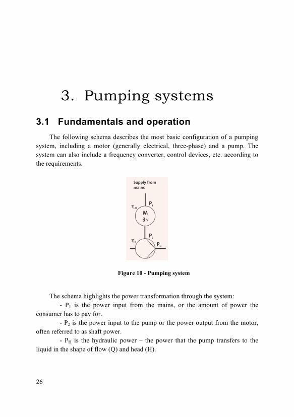
3.1 Fundamentals and operation The following schema describes the most basic configuration of a pumping
system, including a motor (generally electrical, three-phase) and a pump. The system can also include a frequency converter, control devices, etc. according to the requirements.
Figure 10 - Pumping system
The schema highlights the power transformation through the system:
- P1 is the power input from the mains, or the amount of power the consumer has to pay for.
- P2 is the power input to the pump or the power output from the motor, often referred to as shaft power.
- PH is the hydraulic power – the power that the pump transfers to the liquid in the shape of flow (Q) and head (H).

27
As a result, when studying a pump one has to pay attention to several types of terms: hydraulic terms, electrical terms, mechanical terms and liquid properties.
Hydraulic terms The most important hydraulic terms are the flow, the pressure and the head. The flow is the amount of liquid that passes through a pump within a certain
period of time. When one deals with performance readings, one has to distinguish between two flow parameters: the volume flow (Q) and the mass flow (Qm).
The pressure is a measure of force per unit area. One distinguishes between static pressure, dynamic pressure and total pressure. The total pressure is the sum of the static pressure and the dynamic pressure.
The head of a pump is an expression of how high the pump can lift a liquid. Head is measured in meter (m) and is independent on the liquid density. The following formula shows the relation between pressure (p) and head (H): 𝐻 =
𝑝𝜌 𝑔
[1]
where : H is the head in [m] p is the pressure in [Pa = N/m2] ρ is the liquid density in [kg/m3] g is the acceleration of gravity in [m/s2]
Figure 11 - hydraulic system

28
The pump head is determined by reading the pressure on the flanges of the pump p2, p1 (see Figure 11) and then by converting the values into head. However, if a geodetic difference in head is present between the two measuring points, as it is the case in figure 11, it is necessary to compensate for the difference. Furthermore, if the port dimensions of the two measuring points differ from one another the actual head has to be corrected for this as well.
The actual pump head is calculated by the following formula:
𝐻 =𝑝! − 𝑝!𝜌 𝑔
+ ℎ! − ℎ! + 𝜈! − 𝜈!2𝑔
[2]
where : H is the actual pump head in [m] p is the pressure at the flanges in [Pa = N/m2] ρ is the liquid density in [kg/m3] g is the acceleration of gravity in [m/s2] h is the geodetic height in [m] v is the liquid velocity in [m/s] The liquid velocity 𝜈 is calculated by:
𝜈 =4.𝑄𝜋 𝐷!
[3]
where: v is the velocity in [m/s] Q is the volume flow in [m3/s] D is the port diameter in [m]
Electrical terms The most important electrical values are the power consumption, the voltage,
the current, and the power factor. Like pressure drives flow through a hydraulic system, voltage drives a
current (I) through an electrical circuit. Normally, pumps are supplied with AC voltage supply. The layout of AC mains supply differs from one country to another. However, the most common layout is four wires with three phases (L1, L2, L3) and a neutral (N). Besides these four wires, a protective earth connection (PE) is added to the system as well. For a 3x400 V/230 V mains supply, the

29
voltage between any two of the phases (L1, L2, L3) is 400 V. The voltage between one of the phases and neutral (N) is 230 V.
For the most common pump types, the term power consumption normally refers to the shaft power, e.g. P2 described above. For pumps with standard AC motors, the power input, e.g. P1, is found by measuring the input voltage and input current and by reading the value cos(j) on the motor/pump nameplate. cos(j) is the phase angle between voltage and current. cos(j) is also referred to as power factor (PF). The power consumption P1 can be calculated:
- for a AC single-phase motor e.g. 1 x 230V 𝑃! = 𝑈 𝐼 𝑐𝑜𝑠𝜑 [4]
- for a AC three-phase motor 1 x 230V 𝑃! = 3 𝑈 𝐼 𝑐𝑜𝑠𝜑 [5]
The QH-curve The QH-curve shows the head, which the pump is able to perform at a given
flow (blue curve).
Figure 12 - A typical QH-curve for a centrifugal pump

30
The red curve is the (hydraulic) system’s characteristic curve which describes
the relation between flow Q and head H in the system. The system’s characteristic curve depends on the type of system in question. One can distinguish between two types:
• Closed systems are circulating systems like heating or air-conditioning systems, where the pump has to overcome the friction losses in the pipes, fittings, valves, etc. in the system.
• Open systems are liquid transport systems like water supply systems. In such systems the pump has to deal with both the static head and overcome the friction losses in the pipes and components.
Open and closed systems consist of resistances (valves, pipes, heat exchanger, etc.) connected in series or parallel, which altogether affect the system characteristic.
When the system’s characteristic is drawn in the same system of co-ordinates as the pump curve, the duty point of the pump can be determined as the point of intersection of the two curves:
The pump curve can be approximated with the following equation:
𝐻 = 𝐻!"# −𝑄𝑄!
!
(𝐻!"# − 𝐻!) [6]
where Qn is the nominal or design flow rate, Hn the nominal head and Hmax
the maximum head. All these parameters come from pump specification given by the supplier.
The same kind of approximation can be done for the system curve.
The η-curve The efficiency is the relation between the supplied power and the utilized
amount of power (Figure 13). In the world of pumps, the efficiency ηp is the relation between the power, which the pump delivers to the water (PH) and the power input to the shaft (P2 ):
𝜂! =𝑃!𝑃!
= 𝜌 𝑔 𝑄 𝐻𝑃! 3600
[7]
where: ρ is the density of the liquid in kg/m3,

31
g is the acceleration of gravity in m/s2, Q is the flow in m3/h H is the head in m
Figure 13 - The efficiency curve of a typical centrifugal pump
The P2-curve The relation between the power consumption of the pump and the flow is
shown in Figure 14. The P2-curve of most centrifugal pumps is similar to the one in Figure 14 where the P2 value increases when the flow increases. 𝑃! =
𝜌 𝑄 𝐻 𝑔3600 𝜂!
[8]

32
Figure 14 - The power consumption curve of a typical centrifugal pump
Control of a pumping system The four main ways to control a pumping system are ON/OFF control, throttle control, bypass control and variable speed drive:
• ON/OFF control is the most rudimentary type of control and consists of a simple bang-bang control.
• Throttle control consists in controlling the flow through a valve placed in series with the pump.
• Bypass control consists in controlling the flow through a valve placed in parallel with the pump.
• Finally, using a variable speed drive is the most efficient method, since it allows a full control of the motor of the pump using a frequency converter.
Energy efficiency audit of a pumping system Figures 15 and 16 presents the standard tool to carry out an energy efficiency audit for a pumping system used in the industry at this day. This is a first approach to compute the power consumption of the pumping system based on nominal data.

33
Figure 15 - Pump save tool inputs
Nominal data regarding the pump and the motor are entered, as well as the type of control used for the pump. The power consumption for each type of control can be estimated using nominal data and an estimation of the flow.
The mechanical power or shaft power at the nominal point P2,n is computed as

34
𝑃!,! = 𝜌 𝑄! 𝐻! 0.981
𝜂! [9]
where 𝜌 is the density of the pumped liquid and 𝜂! is the efficiency of the pump at the nominal operating point. The power consumption is estimated from empirical derived formulations according to the control type. With a variable speed drive:
𝑃!"# ! = 𝜌 𝑄! 𝐻! 9.81
𝜂! 𝜂! 𝜂!"# 𝑘!" 𝑘!"#$ [10]
where
𝑘!" = (𝑄!𝑄!)(!.!!!.! !!"/!!) [11]
and𝑘!"#$ can be found in an empirical table.With throttle Control:
𝑃!! ! =
𝜌 𝑄! 𝐻!" 9.81𝜂! 𝜂! 𝑘!"
[12]
where
𝑘!" = 𝑄! (2.4 − 1.44
𝑄!𝑄!
)/𝑄! [13]
With ON/OFF Control:
𝑃!"/!"" !"# = 𝜌 𝑄! 𝐻! 9.81
𝜂! 𝜂! [14]
An estimation of the flow profile (e.g. time split of the flow at which the
pump is operated) is entered by the user, as well as some economic data regarding energy cost. The energy consumption can then be estimated, as well as the savings that could be done using different types of control – mainly variable-speed drive.

35
Figure 16 - Pump save tool outputs
3.2 Academic state-of-the-art for pumping systems operation
Since it represents an important proportion of the global energy consumption, pumping systems have been the topic of many research projects. Most of them deal with monitoring of the system, mainly for state estimation and condition monitoring, and with optimization of the operation.

36
Operational state estimation Being able to identify the state of a pumping system is the first step towards a
better operation, but it requires a lot of measurements. Recent methods developed aims at getting over the lack of sensors [1] and advocates model-based methods [3]. Frequency convertors, more and more frequent on the field, are also a new tool for state estimation [2].
Performance monitoring Performance monitoring of a pumping system can be seen as a further state
estimation. Methods developed use the same approaches: - using a frequency converter [4] - using model-based methods and first principles [5], [6], [7] - using data-driven methods [16]
Condition monitoring Condition monitoring of a pumping system is much more complex than
performance monitoring; literature is therefore much more luxuriant. Methods often require hard to get measurement such as vibration of the pump. As a result good condition monitoring is difficult to implement in the frame of this thesis. Interesting methods such as [12] or [15] can still be mentioned.
Statistical modelling Modelling of a pumping system is also an important field of study, since it is
closely related to the optimization problem. Latest research can be found in [14], [18], [19] and [20].
Operation optimization and optimal scheduling Operation optimization and optimal scheduling are key topics for pumping
systems, both for the operation of a single pump or a system (series, parallel) of pumps. [8], [13], [21], [22], [23] addresses different methods of optimization.

37
3.3 Pumping systems operation in an industrial context
Most papers mentioned in Section 3.3 depicts methods tested in optimal conditions regarding data availability. On Oil and Gas and Chemical plants, data availability is a critical issue. The number of measurements is limited and most of them are local, e.g. cannot be used for monitoring. In addition to that, unclear structure of the databases sometimes prevents data from being used. As a result, most methods described previously cannot be used in an operational context, and solutions on the market are considerably different. This is one of the main reasons why KPIs appear as a relevant solution to monitor pumping systems.

38
4. KPIs for pumping systems
4.1 Plant operation data The study has been carried out on historical datasets from different petrochemical plants. It is important to study different plant topologies in order to get a relatively broad view of the data generally available for pumps.
The retained dataset for the study contains the data available in the process historian from the Distributed Control System (DCS), the alarm logs as well as the relational tables to define the structure of the database.
The data available from the DCS features: - 1376 variables sampled every minute - 1 comma separated values (csv) file per day (~ 10 MB) - 2 months of available data (i.e. ~ 600 MB) - P&IDs & Process Descriptions The relational tables link tags, process measurements, equipment description,
alarms descriptions, etc. The alarm logs features 1 csv file per day including all the alarms of the plant.
4.2 Extracting the data Extracting the relevant data is a critical stage when dealing with plant asset management. There is an important number of assets that have to be dealt with according to their type, and the information related to a certain asset is very often not straightforward to get. The structure of the database in the process historian is a key element to be able to extract the data, e.g. defining which process measurements are related to which assets, which nominal data are related to which asset, which events are related to which assets, etc. as well as linking all the tag names to physical values. Thus, according to the structure of the database, a

39
certain search function can be defined to extract relevant data. Figure 17 shows the web interface of such a search function designed by another student at ABB’s Corporate Research Centre for the plant studied in the frame of this thesis.
Figure 17 - Web interface for the search function defined for this plant
However, in most cases the structure of the database alone is not enough to carry out a perfect clustering of the data and information is lost. An extensive manual review has to be done using a process approach, that is based on the P&IDs of the plant. It includes by definition:
• all the assets and their IDs, • all the process measurements and their IDs, and • all the design and nominal information regarding the assets. In the case of the dataset mentioned in Section 4.1, the search function
approach led to approximately a half of the process measurements that could be found using the P&IDs.
There are a several other approaches that can be used to cluster the data available. Semantic clustering can be implemented to cluster the assets according to their type without supervision. Such methods have also been tested in the frame of this thesis and the results were encouraging.
However, in order to be as exhaustive as possible, the datasets used for the project are the ones obtained though the process approach. Appendix A contains a table summarizing all the most important data available for the different pumps of the plant.

40
4.3 KPIs definition for pumping systems As mentioned earlier, the approach chosen for this project is to define KPIs
based on available historical data. Implementability is a critical factor, and both a first principles approach (from the theory of pumping systems) and a data analysis approach have their merits. Based on the selected dataset presented in Appendix A for a representative fleet of pumps of a petrochemical plant, a set of KPIs have been extracted.
First, the measurements that can be found in the dataset in relation to a certain pump are selected.
Measurements (defined as time series) • Number of operating hours • Motor current • Pressure (input & output) • Flow (input & output) • Temperature (input & output)
Some direct computations led us to another set of time series: Direct Computations (defined as time series) • Delivery Head • Electrical Power • Hydraulic Power
Some important information can also be derived from the distribution (over a certain period of time) of relevant signals:
Distributions • Power distribution • Flow distribution • Delivery Head distribution
These time series and distributions contains a lot of information on the operation of the system but cannot be defined as KPIs according to the ISO 22400 standard definition. The following KPIs be defined based on these signals, defined as single values.

41
KPIs Average • Average current during ON stages
KPIs Consumption • Energy Consumption • Flow Consumption
KPIs Efficiency • Total efficiency • Ratio Energy/ Flow = Energy Performance Indicator • Ratio Cost/Flow = Financial Performance Indicator • Savings if operated with variable speed drive
KPIs Deviation To Design • Deviation to design power • Deviation to nominal flow • Deviation to nominal head • Deviation to Optimal efficiency
KPIs Startups Analysis (mainly for batch process) • Frequency of startups • Average current peak height during startup • Average duration of the current peaks during startup
KPIs Condition (based on the number of operating hours signal) • Mean Time Between Failure • Mean Time To Repair
These KPIs are defined according to the ISO 22400 nomenclature in Appendix B.
4.4 Computing the KPIs KPIs are first computed using Matlab based on the data extracted for the pumps.
Average current during ON stages This KPI is computed from the motor current signal. The ON and OFF stages are first defined according to this signal; for that one can introduce a certain relative threshold for the current under which the motor can be considered to be off (it will

42
never be exactly zero due to noise and measurement errors); a threshold like 5% gives generally good results. An average is then computed for the current over the ON stages.
Energy Consumption The power consumption is computed from the integral of the power time series over a certain period of time, or equivalently from the voltage (entered as a single value or as a time series) and the current measurement using the formula given in the KPI definition.
Flow Consumption The flow consumption is defined as the integral of the flow measurement over a certain period of time.
Total efficiency The total efficiency is computed using the formula given in the KPI definition, e.g. involving the electrical power consumed and the hydraulic power supplied (estimated from the flow and the pressure measurement). It is computed over a certain period of time.
Ratio Energy/ Flow - Energy Performance Indicator This KPI is computed as a ratio between the power time series and the flow time series. It can be computed at time T or as an average over a certain period of time.
Ratio Cost/Flow - Financial Performance Indicator This KPI is computed as a ratio between the power time series (integrating the energy cost) and the flow time series. It can be computed at time T or as an average over a certain period of time.
Savings if operated with variable speed drive The savings with variable speed drive can be estimated using the method described in the pump save tool in Section 3.2. Based on the flow distribution (over time) that can be computed from the flow measurement, and on the nominal data detailed in Section 3.2, an estimation of the annual savings with a variable speed drive can be estimated in terms of energy or cost.

43
Deviation to design power The deviation to the design power is computed from the power time series using the design power of the pump given in the P&IDs. It can be computed at time T or as an average over a certain period of time.
Deviation to nominal flow The deviation to the design flow is computed from the flow time series using the design flow of the pump given in the P&IDs. It can be computed at time T or as an average over a certain period of time.
Deviation to nominal head The deviation to the design head is computed from the pressure time series using the design head of the pump given in the P&IDs. It can be computed at time T or as an average over a certain period of time.
Deviation to Optimal efficiency The deviation to the optimal efficiency is computed from the total efficiency using the optimal efficiency of the pump given in the P&IDs. It can be computed at time T or as an average over a certain period of time.
The next three KPIs are computed using the motor current signal based on the phenomenon of current peak during each startup of the pump. The Matlab function findpeaks used is described below.
[pks, locs, w]= findpeaks(data,'MinPeakProminence',15,'MinPeakDistance',100,'Annotate','extents','WidthReference','halfheight')
where the inputs are: • data: the motor current measurement• 'MinPeakProminence': defines the minimum prominence of the
peaks that the function will return.• 'MinPeakDistance': defines the minimum distance between the
peaks that the function will return.
and the outputs : • pks : defines the local maxima (peak)

44
• locs : defines the location of the peak• w : defines the width of the peak
The function is tuned and applied to the current signal.
Frequency of startups The frequency of startups is defined as the number of peaks returned by the findpeaks function and divided by the time period.
Average current peak height during startup The average current peak height is defined as the average height of the peaks returned by the findpeaks function.
Average duration of the current peaks during startup The average duration of the peak is defined as the average width returned by the findpeaks function.
The mean time to failure and mean time between failure can be estimated
using the number of operating hours signal associated with the pump. It is implemented as a an incremental counter that is running when the pump is in operation. As a result one can suppose that when the counter stays constant, the pump is in some way or another facing a technical issue that prevents it from being run. The spare pump, placed in parallel of the main one, is then activated. A failure can thus be detected by a change of slope in the signal as pictured in Figure 18. The duration of the failure is supposed to be equal to the time period on which the main pump signal is constant.

45
Figure 18 - Number of operating hours signal for the main pump (bottom graph)
and the spare pump (upper graph).
Mean Time Between Failure The mean time between failure is computed as the average duration for which the pump is operated without failure.
Mean Time To Repair The mean time to repair is computed as the average duration for which the pump is off after a failure.

46
5. Implementation
5.1 KPI Application The standard ISO22400 defines a KPI markup language that allows KPIs to
be implemented, stored and exchanged in a standard way. KPIs can thus be written directly in XML and stored as XML files. Once all the KPIs for pumps have been defined as XML files, a KPI configuration tool developed in Decathlon can be used in order to generate instances of this KPIs.
Figure 19 - KPI configuration tool in Decathlon

47
Loading data from the pump KPIs library containing all the KPIML files, this tool allows to generate (and compute) a KPI for a specific pump using the relevant data and stores it in an XML file. Inputs specific to the pump have to be specified (nominal data or measurements) so that the KPI can be computed.
The pump library therefore includes the KPIML files but also all the Matlab routines that these KPIMLs must call in order to process the computations. The Matlab routines are compiled beforehand in dll files in order to be usable directly.
KPIs defined through the KPI configuration tool (KPI instances) can then be
displayed and monitored in the main dashboard of the software. The search function allows to access the predefined KPIs.
Figure 20 - Example of KPI - deviation to design power for a pump displayed at
time T

48
Figure 21 - Example of KPI - deviation to design power for a pump monitored over a certain period of time
5.2 Pump Application While the pump KPIs library is a first direct implementation of the work presented in Section 4, another approach would be to adopt an asset point of view and, building on the data analysis stage carried out on historical operational datasets, to design a pump specific application gathering all the relevant information associated with it.
Concept The concept of the pump application is presented in Appendix C.
The faceplate constitutes the technical datasheet of the asset and includes all the nominal and technical details of the pump that can be found from the P&IDs in the database of the plant. The trends part offers to display all the process measurements associated with the asset as well as important values that can derived directly such as the delivery

49
head, the electrical power consumed and the hydraulic power supplied. The deviations from the design parameters (deviation to design power, deviation to nominal flow, deviation to nominal head, deviation to optimal efficiency) can also be displayed as trends. The power distribution, the flow distribution, and the delivery head distribution, which contain particularly relevant information on how the pump is being run are displayed too. The notes part and the alarms part gather all the events that can be found in the historian of the DCS that may be linked to this particular pump according to the search function previously defined – e.g. that may contain the tag name of the asset. These events can be automatically generated or manually entered by the operators. Finally the KPI part lists all the most important KPIs defined as single values (over a certain period of time).
Realization The concept of the pump application has been implemented in Decathlon for the plant selected. First of all, similarly than for KPIs, pumps have to be defined as pump instances of a pump object. This way, information (nominal and design values, references of the related process measurements) can be stored and easily modified by the operators The structure used is a simple spreadsheet (type Microsoft Excel).
The application is developed in a .NET framework and information is read directly from the spreadsheet. The different pumps listed in the plant can be found using a search bar (see Figure 22), and one can access the pump application of a particular pump by drag and dropping to the dashboard.

50
Figure 22 – Faceplate of the selected pump
The first page that appears (Figure 22) is the faceplate of the pump. It displays all the technical details of the selected pump that can be found in the different data files of the plant, according to the concept mentioned earlier.

51
Figure 23 – Energy monitor of the pump
The second page one can access (figure 23) is the an energy monitor of the pump. It shows the energy related KPIs which can be computed for the selected pump over the selected period of time. The graph displays the power signal as well as the design power, and the power distribution over time is presented on the right. The user can navigate over time using a rollover cursor and recompute the different indicators on the new time period though the interact mode accessible on the left of the screen. The “back in time” mode allows to navigate back in time in the process measurement to troubleshoot possible malfunctioning.

52
Figure 24 - Flow monitor of the pump
The third page (Figure 24) is the flow monitor of the pump. The flow is the
expected output of the pump and it is critical to monitor for the operator. The relevant KPIs are computed above and the distribution is displayed on the right. “Interact” and “back in time” mode cover the same features as for the energy monitor.

53
Figure 25 - Process measurements related to the selected pump
The fourth page gathers all the process measurements associated with the pump and basic indicators are computed.

54
Figure 26 - KPIs page
The final page contains all the KPIs which can be computed for the selected pump. Energy and flow KPIs are presented once again, as well as others.

55
6. Discussion and Further Development
6.1 Towards a pumpML language The need for information about pumps to be stored in pump “objects” has
been mentioned in Section 5.4. When implemented in Decathlon, this was done using a spreadsheet format gathering all the information related to the pumps of the plant. While this solution presents the advantage of being convenient and straightforward to modify for the newcomer, it features a serious lack of competitiveness when compared with a markup language such as the one that has been defined for KPIs. In that perspective, the introduction of an assetML language seems particularly relevant.
The structure of the pumpML language would include all the fields that are related to a pump object, according to the concept of object-oriented engineering which is more and more advocated in the literature. In a brief overview, the pumpML structure would feature:
• the basic information of the pump (nominal and design values, technical details, etc.),
• the relevant process measurements for a pump, • the notes, • the alarms, and • the KPI defined in the pump KPIs library.
Once this structure has been formalized it is possible to generate instances for all the pumps that can be found in the plant. These instances, as KPI instances do, contain the information for the pump selected that is available, and the reference to the tag names of the available measurements as well as references to the

56
computable KPIs. These instances carry the information of the pump, but the data (measurements, KPIs) is stored somewhere else.
Integration of the pumpML and KPIML approaches One of the main issue that can be faced when defining a pumpML object
with this structure is the integration between the pumpML and the KPIML approaches. Indeed, when defined in the pump object, pump KPIs are designated as they have been defined as KPI objects. However, when the pump is instantiated, the KPIs fields have to be filled with instances of KPIs. As a result, pump KPIs have to be instantiated totally independently of the pump instance – but based on the same process measurements defined in the pump instance. This raises an important conceptual problem that prevents the pumpML approach to be implemented in a proper way for the user.
On the other hand, if the pumpML structure is implemented such as KPIs are directly defined in the pump object in the same way as they are defined in the KPI object, then computation can be processed without requiring the generation of KPI instances. Nevertheless, in this case KPIs defined in the pump object will not be available as KPIs object, and thus impossible to monitor independently for the user.
6.2 Extending the approach to other assets: asset KPI library and assetML
The aim of this thesis was to define and test an asset specific KPI library, as well as to place it as far as possible in an asset markup language that would regulate the storage and the exchange of information in a standard way building on the concept of object-oriented engineering. An overwhelming part of the project has been carried out as a case study on a particular type of asset – pumps, because they represent an ideal candidate in the sense that they are the most widely represented asset in the plants (implying a important population to study in a statistical point of view) and they represent one of the highest potential of savings in operations expenditures. However, generalization of the approach to any type of asset is an important topic.
The work carried out on KPIs definition can be extended to any type of asset, e.g. compressors, boilers, heat exchangers etc. For each type of asset, a theoretical study can be lead to the definition of operational KPIs that can be implemented
57
according to the operational data generally available for these assets on the plant. A comprehensive assets KPIs library can thus be established and provide the different audience (operator, supervisor, management) with pre defined tools to build a custom KPI dashboard. The KPIML implementation allows KPIs to be instantiated in a straightforward way and then ready to be monitored anytime.
The definition of an assetML implementation is a much more complex problem, since it has to deal with the heterogeneity of the features of the different types of assets. Therefore defining a non-asset-specific common markup language could require a lot of work but a structure like the one suggested for the pumpML implementation could be an interesting starting point, e.g. :
• the technical details of the asset • the relevant process measurements for the asset • the operator notes related to the asset • the alarms associated with the asset • the KPI defined in the asset KPIs library
However, the degree of generalization of the assetML implementation has still to be defined, according to the use that can be done with it.
6.3 Extending the approach to higher levels: fleet management
The work carried out on pump monitoring and asset monitoring in general has been centered around monitoring of a single asset. It can also be extended to a higher level in order to implement a fleet management feature.
First, synthetizing all the information available for each pump of the plant in the pump application, one can develop an aggregate dashboard to monitor the state of the pump fleet. “Second-level” KPIs can be determined in order to provide an overview of how the fleet is run. A “concept draft” of aggregate dashboard for pumps can be found in Appendix D.
The upper part includes general KPIs that can be used to assess the state of the fleet such as the age of the fleet (through the number of operating hours) and an indicator of how well the pumps are being run (such as the frequency of startups). It includes key trends such as the total energy consumption of the fleet and/or the cost that it represents; this allows the audience to point out what are the global trends of the fleet over representative periods of time. It also allows them to diagnostic global shifts in these values that may not identified on a single asset.

58
The bottom part provides an overview of the individual assets presenting only a couple of most representative KPIs such as the number of operating hours, the frequency of startups or the savings if this particular pump was run with a variable speed drive. The power consumption as a trend can also be displayed, as well as an indicator if the pump is related to an alarm or a note that happened recently. This allows the audience to make a decision about the action to be taken on the fleet at a glance.
The approach described above can be applied to any type of asset once defined the assetML structure. Aggregate dashboards and overviews of the fleet of this asset type can be computed directly from the individual asset monitor based on operational data. As a result, in addition to providing the user with fleet management by asset type it is possible to build a synthetic assets dashboard showing synthetic information about how the different families of assets are operated. Appendix E suggests a “concept draft” of such a synthetic dashboard.
For each type of asset, an OPEX related KPI can be visualized as a trend, e.g. the power consumption for the whole fleet of this type of asset. The cost that it represents can also be displayed. A condition related KPI, chosen according to the type of asset, can also be showed as a trend.
6.4 KPIs as integration between control and scheduling
Another important topic that has been raised during this project is the integration of control and scheduling. Control and scheduling tend to be more and more integrated, but although literature abounds in this sense (see [10] for example), their full integration seems to be actually very difficult to reach. Studying KPIs at the asset level allows to highlight how KPIs could serve as vectors for this integration. As an illustrating example, a KPI for start and stop analysis of batch processes based on the current signal of the motor of the pump is presented. The KPI has been designed in the frame of this thesis and is described in [29].
The idea of the paper is to claim that some KPIs defined by the ISO 22400 standard may be used as outputs of the scheduling system and computed taking inputs both from the scheduling system and from the DCS. Since these KPIs are monitored and used as primary variables for feedback and action on the production system, they represent a vector of integration of the scheduling system and the DCS.

59
One of the examples chosen in the paper is the effectiveness of an asset or a work unit that can be defined by the product of the planned runtime per item (which is a direct output of the scheduling system) multiplied by the produced quantity in relationship to the actual production time, which can be measured using the process measurement associated with the equipment in the DCS.
Using the current measurement of the motor of a pump, it is possible to compute the actual production time for a batch process. The method developed in the frame of this thesis, and described in the paper, is recalled below.
Step 1. Convert the current signal to a binary signal in order to determine whether the motor is switched on (above a defined threshold) or off (below the threshold). The current will never drop to zero due to measurement errors and artefacts.
yi =1 𝑥! ≥ 𝜃 0 𝑥! < 𝜃 [15]
Step 2. Eliminate short periods where the motor is switched off since these periods do not constitute the change between two batches.
yi =1 𝑦! = 1 δi 𝑦! = 0 [16]
where δi is defined as
𝛿! =1 𝑖: 𝑘!"",!"# − 𝑘!"",!"#$" > 𝐾! δi 𝑖: 𝑘!"",!"# − 𝑘!"",!"#$" ≤ 𝐾!
[17]
𝑘!"",!"#$" is the start of the off period and 𝑘!"",!"# is the end of the off period within the sample i lies. Kδ is the length below which an off period is considered
insignificant.
Step 3. Eliminate short periods where the motor is switched on since these periods

60
do not constitute a change between two batches.
yi =𝜀! 𝑦! = 1 0 𝑦! = 0 [18]
where εi is defined as
𝜀! =
1 𝑖: 𝑘!",!"# – 𝑘!",!"#$" > 𝐾!0 𝑖: 𝑘!",!"# – 𝑘!",!"#$" ≤ 𝐾!
[19]
𝑘!",!"#$" is the start of the on period and 𝑘!",!"#is the end of the on period within
the sample i lies. 𝐾! is the length below which an off period is considered insignificant.
Figure 27 - Start and stop analysis of batches using the pump’s motor current
signal

61
Figure 27 shows the implementation of the method in Matlab. Red lines represent the start of the batches and green lines represent the end. The actual production time can then be computed and any action that can be taken in order to improve the effectiveness of the asset or the work unit has to consider both the outputs of the scheduling system and the inputs of the DCS.

62
7. Conclusion Building on the ISO 22400 standard on KPIs for manufacturing operations management, the initial idea of this project was to test the KPI approach at the asset level, defining a standard set of KPIs (or a library) associated with a certain type of asset and taking into account the data generally available in the different information systems of the plant. In order for the project to be operationally significant, a major part of the study has been carried out as a case study on a particular type of asset – pumping systems – using historical data from petrochemical plants.
The pump KPI library has been defined using the standard developed in ISO 22400; the KPIs have then been implemented in Matlab and compiled to be used in ABB’s new operations management software, Decathlon. The pump KPI library has been defined using a KPIML implementation in order for it to be instantiated easily through the KPI configuration tool, and then monitored in the KPI dashboard for the pumps of the selected plant.
The work on KPIs has been taken further by the creation of a pump application designed to monitor all the information available in the databases that are linked to the selected pump. Including all the data that had been identified in the data analysis stage of the project (technical details of the pump, operator notes, alarms, process measurements), the application relies to a large part on the KPIs defined previously for pumps. The application has been implemented in Decathlon as one of the first applications to be implemented in the software, and as a prototype for “asset monitoring application”.
The pump application raises the question of a pump mark-up language that would allow to store and exchange the information related to pumps in a standard way. The topic has been studied in the frame of the project, but no definite standard implementation has been defined, mainly due to the issues raised by the integration with the KPIML implementation.
63
All the work carried out in the frame of the case study on pumps is intended to be extended to any type of asset. Asset-specific KPI libraries could be developed for each type of asset based on data generally available on the plants. Asset monitoring applications can thus be designed based on the scheme “Technical details of the asset – Relevant process measurements – KPIs defined for the asset”. Such a structure would lay a common ground for a potential asset mark-up language implementation and would allow asset monitoring applications to be taken to a higher level to introduce a fleet management feature. Such ideas have been discussed in the frame of the project but their further development and/or their implementation would have gone beyond the initial scope of the project, and the time required far beyond the time accorded for the project.

64
Bibliography 1. Ahonen, T., Tamminen, J., Ahola, J., & Kestilä, J. (2009,
September). Sensorless pump operation estimation. In Power Electronics and Applications, 2009. EPE'09. 13th European Conference on (pp. 1-10). IEEE.
2. Ahonen, T., Tamminen, J., Ahola, J., & Kestilä, J. (2012). Frequency-converter-based hybrid estimation method for the centrifugal pump operational state. Industrial Electronics, IEEE Transactions on, 59(12), 4803-4809.
3. Ahonen, T., Tamminen, J., Ahola, J., Viholainen, J., Aranto, N., & Kestilä, J. (2010). Estimation of pump operational state with model-based methods.Energy Conversion and Management, 51(6), 1319-1325.
4. Ahonen, T., Tiainen, R., Viholainen, J., Ahola, J., & Kestilä, J. (2008, June). Pump operation monitoring applying frequency converter. In Power Electronics, Electrical Drives, Automation and Motion, 2008. SPEEDAM 2008. International Symposium on (pp. 184-189). IEEE.
5. Attivissimo, F., Di Febo, M., Paganini, P., & di Mango, G. (2014, September). Model based control and diagnostic system for centrifugal pumps. InEnvironmental Energy and Structural Monitoring Systems (EESMS), 2014 IEEE Workshop on (pp. 1-6). IEEE.
6. Bae, C. O., Vuong, D. P., & Park, Y. S. (2012, November). Pump efficiency instrumentation based on thermodynamic method and traditional technique. InControl, Automation and Information Sciences (ICCAIS), 2012 International Conference on (pp. 359-363). IEEE.
7. Cicciotti, M., Xenos, D. P., Bouaswaig, A. E., Thornhill, N. F., & Martinez-Botas, R. F. (2014, June). Online Performance Monitoring of Industrial Compressors Using Meanline Modelling.

65
In ASME Turbo Expo 2014: Turbine Technical Conference and Exposition (pp. V02DT42A003-V02DT42A003). American Society of Mechanical Engineers.
8. da Costa Bortoni, E., de Almeida, R. A., & Viana, A. N. C. (2008). Optimization of parallel variable-speed-driven centrifugal pumps operation. Energy Efficiency, 1(3), 167-173.
9. Discenzo, F. M., Rusnak, D., Hanson, L., Chung, D., & Zevchek, J. (2002). Next generation pump systems enable new opportunities for asset management and economic optimization. In PROCEEDINGS OF THE INTERNATIONAL PUMP USERS SYMPOSIUM (pp. 9-16).
10. Engell, S., & Harjunkoski, I. (2012). Optimal operation: Scheduling, advanced control and their integration. Computers & Chemical Engineering, 47, 121-133.
11. Hao, H., & Shaanxi, V. R. Key Performance Monitoring and Diagnosis in Industrial Automation Processes.
12. Kleinmann, S., Stetter, R., Prasad, K., & Kumar, P. (2013, October). Optimization of a pump health monitoring system using fuzzy logic. In Control and Fault-Tolerant Systems (SysTol), 2013 Conference on (pp. 251-256). IEEE.
13. Kopanos, G. M., Xenos, D. P., Cicciotti, M., Pistikopoulos, E. N., & Thornhill, N. F. (2015). Optimization of a network of compressors in parallel: Operational and maintenance planning–The air separation plant case. Applied Energy, 146, 453-470.
14. Kusiak, A., Zeng, Y., & Zhang, Z. (2013). Modeling and analysis of pumps in a wastewater treatment plant: A data-mining approach. Engineering Applications of Artificial Intelligence, 26(7), 1643-1651.
15. Li, X., Du, R., & Guan, X. P. (2004). Utilization of information maximum for condition monitoring with applications in a Machining Process and a water pump. Mechatronics, IEEE/ASME Transactions on, 9(4), 711-714.
16. Marzi, H. (2005, June). Reconfigurable multi-stage neural networks in monitoring industrial machines. In Soft Computing in Industrial Applications, 2005. SMCia/05. Proceedings of the 2005 IEEE Mid-Summer Workshop on (pp. 142-147). IEEE.
17. Sun, Q. (2012, October). Research and design of the computer-aided selection system of the circulation pump based on the performance curve. In System Science, Engineering Design and

66
Manufacturing Informatization (ICSEM), 2012 3rd International Conference on (Vol. 1, pp. 150-153). IEEE.
18. Xenos, D. P., Cicciotti, M., Bouaswaig, A. E., Thornhill, N. F., & Martinez-Botas, R. (2014, June). Modeling and optimization of industrial centrifugal compressor stations employing data-driven methods. In ASME Turbo Expo 2014: Turbine Technical Conference and Exposition (pp. V03BT25A004-V03BT25A004). American Society of Mechanical Engineers.
19. Xenos, D. P., Thornhill, N. F., Cicciotti, M., & Bouaswaig, A. E. (2014, July). Preprocessing of raw data for developing steady-state data-driven models for optimizing compressor stations. In Control (CONTROL), 2014 UKACC International Conference on (pp. 438-443). IEEE.
20. Zhang, Z., & Kusiak, A. (2011). Models for optimization of energy consumption of pumps in a wastewater processing plant. Journal of Energy Engineering.
21. Zhang, Z., He, X., & Kusiak, A. (2015). Data-driven minimization of pump operating and maintenance cost. Engineering Applications of Artificial Intelligence, 40, 37-46.
22. Zhang, Z., Zeng, Y., & Kusiak, A. (2012). Minimizing pump energy in a wastewater processing plant. Energy, 47(1), 505-514.
23. Zhuan, X., & Xia, X. (2013). Optimal operation scheduling of a pumping station with multiple pumps. Applied Energy, 104, 250-257.
24. ANSI/ISA-95.00.01-2000: Enterprise-Control System Integration, Part 1-5, 2007
25. Hollender, M. (2010). Collaborative Process Automation Systems. ISA.
26. Woll, Dave (2004). Achieving Operational Excellence Through Collaborative Process Automation Systems, ARC Advisory Group
27. Ferman, R., et al., (2008). “Optimizing Pumping Systems”, page XXII. New Jersey: Hydraulic Institute.
28. Merkle , M. (2015) “Optimale Wertschöpfung von Maschinen durch ganzheitliche Betrachtung von Anlagen der Prozessindustrie“
29. Bauer, M., Harjunkoski, I., Lucke, M., Schlake, J. (2016): “KPIs as the Interface between Scheduling and Control”
30. ISO 22400-1 and 2 (2014). Automation systems and integration - key performance indicators (KPIs) for manufacturing operations management – Part 1 and Part 2

67
31. ISO 22400-2 Amendment 1 (2015)— Manufacturing operations Management — Part 2: Key performance indicators for energy management
32. Groenewald, J. (2015), A process performance monitoring methodology for mineral processing plants
33. MESA International, Key Performance Indicator Markup Language, Version 01 - May 2015

68
Appendices

69
Appendix A
Measured Values Nominal Values Other Informations
ID Current
Pressure
Temperature
Flow PH Nominal flow
Nominal head
Design P_in
Design P_out
Design T_in
Design T_out
Material Pumped medium
Voltage
P402A
N6020
T6009 254,4 102 17,5 20 170 200 GS-C 25 Hot base U6000
P402B
N6021
P6018 T6009 254,4 102 17,5 20 170 200 GS-C 25 Hot base U6000
P404A
N6024
P 6019 T6017 150 86 17 20 120 200 GS-C 25 MDEA U6000
P404B
N6025
P 6019 T6017 150 86 17 20 120 200 GS-C 25 MDEA U6000
P406A
N6030
T6018 130 158 26 120 GS-C 25 MDEA U6000
P406B
N6031
T6018 130 158 26 120 GS-C 25 MDEA U6000
P411A
N6107
FI6110
110 21 40 50 120 250 "1.4517" Sauerwasser U6100
P411B
N6108
FI6110
110 21 40 50 120 250 "1.4517" Sauerwasser U6100
P431A
N6305
QI6303
199 41 10 20 GS-C 25 Water U6300
P431B
N6306
QI6303
199 41 10 20 GS-C 25 Water U6300
P432A
N6315
72 79 20 200 GS-C 25 MDEA U6300
P432B
N6316
72 79 20 200 GS-C 25 MDEA U6300
P433A
N6317
7,6 27 8 170 HII 1.0425/ 1.693 GGG40
SCOT U6300
P433B
N6318
7,6 27 8 170 HII 1.0425/ 1.693 GGG41
SCOT U6300
P451A
N6502
FI6502
60 60 16 170 1.0619(GS-C 25)
Schwefelverlader
U6500
P451B
N6503
FI6502
60 60 16 170 1.0619(GS-C 25)
Schwefelverlader
U6500
P462A
N6608
T6613 FI6628
37,8 375 40 120 GS-C 25 Kesselspeisewasser
U6600
P462B
N6609
T6613 FI6628
37,8 375 40 120 GS-C 25 Kesselspeisewasser
U6600

70
Appendix B KPI Definition
Content
Name Average current during ON stages
ID
Description Average current provided to the pump over a certain period of time considering only the time when the pump is ON
Scope
Formula "𝐀𝐯𝐞𝐫𝐚𝐠𝐞 𝐜𝐮𝐫𝐫𝐞𝐧𝐭 𝐝𝐮𝐫𝐢𝐧𝐠 𝐎𝐍 𝐬𝐭𝐚𝐠𝐞𝐬" =𝐈𝐎𝐍𝒊𝒏
𝒊!𝟏
𝐓𝒔𝒕𝒂𝒈𝒆
IONi : average current on ith stage on which the pump is ON Tstage : duration of the stage
Unit of Measure Ampere
Range Min: 0 Max: infinite
Trend
Context
Timing On-Demand or periodically
Audience Operator, supervisor
Production Methodology
Mainly batch process
Effect Model Diagram
Notes

71
KPI Definition
Content
Name Energy Consumption
ID
Description Energy consumption of the pump over a certain period of time.
Scope
Formula 𝐄𝐧𝐞𝐫𝐠𝐲 𝐂𝐨𝐧𝐬𝐮𝐦𝐩𝐭𝐢𝐨𝐧 = 𝑼 ∗ 𝑰 ∗ 𝟑 ∗ 𝒄𝒐𝒔(𝝋) 𝒅𝒕
Defined as the integral of the power signal over a certain period of time
Unit of Measure kWh
Range Min: 0 Max: to be defined
Trend The closer to 0, the better
Context
Timing Online or on-demand.
Audience Operator, supervisor
Production Methodology Discrete, batch, continuous
Effect Model Diagram
Notes

72
KPI Definition
Content
Name Flow Consumption
ID
Description Flow consumption of the pump over a certain period of time.
Scope
Formula 𝐅𝐥𝐨𝐰 𝐂𝐨𝐧𝐬𝐮𝐦𝐩𝐭𝐢𝐨𝐧 = 𝑸 𝒅𝒕
Defined as the integral of the flow signal over a certain period of time
Unit of Measure m3
Range Min: 0 Max: to be defined
Trend The higher, the better
Context
Timing Online or on-demand.
Audience Operator, supervisor
Production Methodology Discrete, batch, continuous
Effect Model Diagram
Notes

73
KPI Definition
Content
Name Overall Efficiency
ID
Description Measured efficiency of the pump
Scope
Formula Overall Efficiency = ηtotal measured= Phydraulic/Pelectrical = Qeff * ∆Hdyn * g * ρ / (U*I*cos(φ)*√3) Phydraulic: hydraulic power provided by the pump Pelectrical: electrical power consumed by the pump Qeff: measured flow as a single value or as a time series ∆Hdyn: measured dynamical head as a single value or as a time series g: gravity constant as a single value ρ: density of the pumped liquid as a single value U: measured voltage as a single value or as a time series I: measured current as a single value or as a time series cos(φ): cos(φ) of the motor as a single value
Unit of Measure -----
Range Min: 0 Max: 1
Trend The higher the better
Context
Timing Online or on-Demand
Audience Operator, supervisor
Production Methodology
Discrete, batch, continuous
Effect Model Diagram
Notes

74
KPI Definition
Content
Name Energy Performance Indicator
ID
Description Single ratio indicator to consider the power required for a certain amount of flow provided by the pump
Scope
Formula Energy Performance Indicator = Power Consumed / Flow provided Power Consumed: power consumed by the pump over a certain period of time (measurement) as a single value Flow provided: flow provided by the pump over a certain period of time (measurement) as a single value
Unit of Measure kWh/m3
Range Min: 0 Max: infinite
Trend The lower the better
Context
Timing On-Demand for a certain period of time or periodically.
Audience Supervisor, management
Production Methodology
Discrete, batch, continuous
Effect Model Diagram
Notes

75
KPI Definition
Content
Name Financial Performance Indicator
ID
Description A single financial indicator in relation to flow
Scope
Formula Financial Performance Indicator = Energy Performance Indicator x Electricity Average Unit Price [€/kWh] Energy Performance Indicator: KPI computed over a certain period of time expressed as a single value Electricity Average Unit Price: Average price of the electricity over the same period of time expressed as a single value
Unit of Measure €/m3
Range Min: 0 Max: infinite
Trend The lower the better
Context
Timing Online
Audience Supervisor, management
Production Methodology
Discrete, batch, continuous
Effect Model Diagram
Notes

76
KPI Definition
Content
Name Savings with variable speed drive
ID
Description Estimation of the savings if the pump was controlled with a variable speed drive instead of the current type of control (generally supposed to be ON/OFF control)
Scope
Formula The KPI is computed using the methods presented in the pump save tool, based on nominal data and on the flow distribution over time. It is computed over a certain period of time.
Unit of Measure Can be expressed in relation to energy savings (in MWh per year for example) or in relation to financial savings (in € per year for example)
Range Min: to be defined Max: to be defined
Trend The lower, the better: it means that the current control of the pump is efficient. Otherwise, it assesses room for potential improvement.
Context
Timing On-demand.
Audience Supervisor, management
Production Methodology
Discrete, batch, continuous
Effect Model Diagram
Notes

77
KPI Definition
Content
Name Deviation to Design Power
ID
Description Evaluation of the distance between the power at which the motor of the pump is operated and its design power.
Scope
Formula Deviation to Design Power =(Pdesign-Pmeasured)/Pdesign Pdesign: Electrical design power of the motor of the pump as a single value or as a constant time series Pmeasured: Measured electrical power consumed by the motor as a time series or as a single value.
Unit of Measure %
Range Min: to be defined Max: to be defined
Trend The closer to 0, the better
Context
Timing Online or on-demand.
Audience Operator, supervisor
Production Methodology
Discrete, batch, continuous
Effect Model Diagram
Notes

78
KPI Definition
Content
Name Deviation to Design Flow
ID
Description Evaluation of the distance between the flow at which the pump is operated and its design flow.
Scope
Formula Deviation to Design Flow=(Qdesign-Qmeasured)/Qdesign Qdesign: Design flow of the pump as a single value or as a constant time series Qmeasured: Measured flow at the output of the pump as a single value or as a time series.
Unit of Measure %
Range Min: to be defined Max: to be defined
Trend The closer to 0, the better
Context
Timing Online or on-demand
Audience Operator, supervisor
Production Methodology
Discrete, batch, continuous
Effect Model Diagram
Notes

79
KPI Definition
Content
Name Deviation to Design Head
ID
Description Evaluation of the distance between the head at which the pump is operated and its design head.
Scope
Formula Deviation to Design Head=(Hdesign-Hmeasured)/Hdesign Hdesign: Design head of the pump as a single value or as a constant time series Hmeasured: Measured head of the pump as a single value or as a time series.
Unit of Measure %
Range Min: to be defined Max: to be defined
Trend The closer to 0, the better
Context
Timing Online or on-Demand
Audience Operator, supervisor
Production Methodology
Discrete, batch, continuous
Effect Model Diagram
Notes

80
KPI Definition
Content
Name Deviation to Optimal Efficiency
ID
Description An indicator of the distance between the measured efficiency of the pump and the optimal efficiency.
Scope
Formula Deviation to Optimal Efficiency = (ηhydraulic optimal* ηmotor optimal - ηtotal
measured)/( ηhydraulic optimal * ηmotor optimal) ηhydraulic optimal: optimal hydraulic efficiency of the pump as a single value or as a time series ηmotor optimal: optimal efficiency of the motor as a single value or as a time series ηtotal measured: total measured efficiency as a single value or as a time series
Unit of Measure %
Range Min: to be defined Max: to be defined
Trend The closer to 0, the better
Context
Timing Online or on-Demand
Audience Operator, supervisor
Production Methodology
Discrete, batch, continuous
Effect Model Diagram
Notes

81
KPI Definition
Content
Name Frequency of start-ups of the pump
ID
Description Number of start-ups of the pump over a certain period of time.
Scope
Formula Frequency of start-ups of the pump = number of start-ups / time period
Unit of Measure /Time period
Range Min: 0 Max: infinite
Trend The lower the better
Context
Timing On-Demand or periodically
Audience Operator, supervisor
Production Methodology
Mainly batch process
Effect Model Diagram
Notes
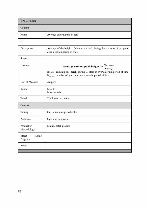
82
KPI Definition
Content
Name Average current peak height
ID
Description Average of the height of the current peak during the start-ups of the pump over a certain period of time
Scope
Formula "𝐀𝐯𝐞𝐫𝐚𝐠𝐞 𝐜𝐮𝐫𝐫𝐞𝐧𝐭 𝐩𝐞𝐚𝐤 𝐡𝐞𝐢𝐠𝐡𝐭 " = 𝐈𝐡𝐞𝐢𝐠𝐡𝐭𝒊𝒏𝒊!𝟏
𝐍𝒔𝒕𝒂𝒓𝒕𝒖𝒑𝒔
IHeighti : current peak height during ith start-up over a certain period of time Nstartups : number of start-ups over a certain period of time
Unit of Measure Ampere
Range Min: 0 Max: infinite
Trend The lower the better
Context
Timing On-Demand or periodically
Audience Operator, supervisor
Production Methodology
Mainly batch process
Effect Model Diagram
Notes

83
KPI Definition
Content
Name Average current peak duration
ID
Description Average of the duration of the current peak during the start-ups of the pump over a certain period of time
Scope
Formula "𝐀𝐯𝐞𝐫𝐚𝐠𝐞 𝐜𝐮𝐫𝐫𝐞𝐧𝐭 𝐩𝐞𝐚𝐤 𝐝𝐮𝐫𝐚𝐭𝐢𝐨𝐧 " = 𝐓𝐩𝐞𝐚𝐤𝒊𝒏𝒊!𝟏
𝐍𝒔𝒕𝒂𝒓𝒕𝒖𝒑𝒔
Tpeaki : current peak duration during ith start-up over a certain period of time Nstartups : number of start-ups over a certain period of time
Unit of Measure Time unit
Range Min: 0 Max: infinite
Trend The lower the better
Context
Timing On-Demand or periodically
Audience Operator, supervisor
Production Methodology
Mainly batch process
Effect Model Diagram
Notes

84
KPI Definition
Content
Name Mean operating time between failures (MTBF)
ID
Description The mean operation time between failures is calculated as the mean of all time between failure measures (TBF) for a work unit for all failure instances (FE).
Scope Work unit
Formula 𝐌𝐓𝐁𝐅 =
𝑻𝑩𝑭𝒊𝒏𝒊!𝟏
𝑭𝑬 + 𝟏
Unit of Measure Time unit
Range Min: 0 Max: infinite
Trend The higher, the better
Context
Timing On-demand, periodically
Audience Supervisor, management
Production Methodology
Discrete, batch, continuous
Effect Model Diagram
Notes Mean operating time between failures (MTBF) is an indicator of expected system reliability calculated on a statistical basis from the known failure rates of various components of the work unit. It represents the expectation of the operating time between failures. It is a statistical approximation of how long a work unit should last before failure. MTBF numbers are usually stated in terms of hours. The indicator is calculated in each work unit. Every time a failure happens, a new TBF is obtained to calculate the MTBF. The MTBF is the sum of MTTR and MTTF.

85
KPI Definition
Content
Name Mean time to repair (MTTR)
ID
Description Mean time to repair (MTTR) is the average time that an item required to restore a failed component in a work unit. The mean time to repair is calculated as the mean of all time to repair measures (TTR) for a work unit for all failure events (FE).
Scope Work unit
Formula 𝐌𝐓𝐓𝐑 =
𝑻𝑻𝑹𝒊𝒏𝒊!𝟏
𝑭𝑬 + 𝟏
Unit of Measure Time unit
Range Min: 0 Max: infinite
Trend The higher, the better
Context
Timing On-demand, periodically
Audience Supervisor, management
Production Methodology
Discrete, batch, continuous
Effect Model Diagram
Notes Mean time to repair (MTTR) is the average time that an item required to restore a failed component in a work unit. It represents the expectation of the time to repair. MTTR numbers are usually stated in terms of hours. The indicator is calculated in each work unit. Every time a failure has been restored, a new TTR is obtained to calculate the MTTR.

86
Appendix C

87
Appendix D

88
Appendix E

Lund UniversityDepartment of Automatic ControlBox 118SE-221 00 Lund Sweden
Document nameMASTER´S THESISDate of issueFebruary 2016Document NumberISRN LUTFD2/TFRT--6001--SE
Author(s)
Matthieu LuckeSupervisorMargret Bauer, ABB AG, Corporate Research CentreCharlotta Johnsson, Dept. of Automatic Control, Lund University, SwedenKarl-Erik Årzén, Dept. of Automatic Control, Lund University, Sweden (examiner)Sponsoring organization
Title and subtitle
KPIs for Asset Management : A Pump Case Study
Abstract
The integration of multiple data sources and the convergence of process control systems and business intelligence layer such as the enterprise resource planning (ERP) are paving the way for important progress in plant operation optimization. Numerous companies offer “Analytics Services” to leverage this newly available mine of data but applications still appear to be limited to certain specific types oflarge plants. Key Performance Indicators (KPIs) is arguably the most used approach to make sense of large and complex systems in a wide variety of fields and its applicability to industrial operations is more and more common, to the extent that standardization of KPIs has become a major topic for the International Organization for Standardization (ISO). While the KPI standard ISO 22400 focuses on KPIs for manufacturing operations management at the plant level, the scope of this thesis is to bring it to the first layer of the control system: the equipment.In addition to being part of the quest for operational excellence and energy efficiency, bringing KPIs
to the asset level is an important step towards integration of the different layers of the automationpyramid, integrating in particular control and scheduling. Developed within the frame of the newgeneration of Operations Management Software for the process industries, this work presents a case study on the most widely used assets in the field – pumps, based on operational data of differentplants in the Oil & Gas and Chemicals industries.
Keywords
Classification system and/or index terms (if any)
Supplementary bibliographical information
ISSN and key title0280-5316
ISBN
LanguageEnglish
Number of pages1-88
Recipient’s notes
Security classification
http://www.control.lth.se/publications/