Norwegian University of Life Sciences

Department of Chemistry, Biotechnology and Food Science

PHILOSOPHIAE DOCTOR THESIS 2008:1

Reliable prediction and determination of Norwegian

lamb carcass composition and value

Pålitelig bestemmelse av sammensetningen i norske lammeslakt og verdi nedskåret vare

Jørgen Kongsro

ISBN 978-82-575-0798-5

ISSN 1503-1667

TABLE OF CONTENTS

PREFACE ................................................................................................................ii

SUMMARY ............................................................................................................iii

OPPSUMMERING (Summary in Norwegian) .............................................................. iv

LIST OF PAPERS ..................................................................................................... v

Background and motivation......................................................................................... 1

Dissection, cutting and value of cuts from lamb carcasses ................................................ 5

Classification of lamb and sheep carcasses; the EUROP classification system..................... 8

Measuring systems for lamb carcass composition ......................................................... 11

Multivariate calibration............................................................................................. 22

Main results of papers I-V and future perspectives. ....................................................... 28

References .............................................................................................................. 31

PAPERS I - V

PREFACE

This work was sponsored by grant 162188 of the Norwegian Research Council, as a part of a

Ph. D. study program. The Ph.D. study is a part of a research project at Animalia – Norwegian

Meat Research Centre, which among other activities is also devoted to optimizing

classification and grading of Norwegian lamb carcasses. The main area of activity for

Animalia is to conduct generic work funded by a farmer Research and Development levy. The

classification and grading system in Norway is supervised by Animalia, but the system is

owned by Nortura BA. Nortura BA has served as an industry partner in this project, and has

provided the sampled carcasses from different abattoirs located in southern Norway.

I would like to thank my supervisors at Norwegian University of Life Sciences, Prof. Are

Aastveit, Associate Prof. Knut Kvaal and last but not least, my main supervisor, Prof. Bjørg

Egelandsdal, who’s scientific and administrative skills, experience and valuable opinions have

guided me through this work to a higher academic level. Morten Røe at Animalia is

acknowledged for his practical and universal skills concerning the meat industry, carcass

classification and dissection, and for providing data and advice, and guiding me through this

work on a pragmatic level. The butchers at Animala are acknowledged for their skills in

dissection of carcasses, and for showing me the art of cutting and dissection of carcasses. Tor

Arne Ruud, Dr. Ole Alvseike and Per Berg are acknowledged for their support and help

during start-up of the project. Dr. Mohamed Kheir Omer Abdella is gratefully acknowledged

for his editing support. I would also like to thank the Norwegian Research Council for

funding this work (grant 162188).

I would also like to thank my family and friends, and especially my wife Tone for her love,

support and motivation during this work.

SUMMARY

The main objective of this work was to study prediction and determination of Norwegian

lamb carcass composition with different techniques spanning from subjective appraisal to

computer-intensive methods. There is an increasing demand, both from farmers and

processors of meats, for a more objective and reliable system for prediction of muscle (lean

meat), fat, bone and value of a lamb carcass. When introducing new technologies for

determination of lamb carcass composition, the reference method used for calibration must be

precise and reliable. The precision and reliability of the current dissection reference for lamb

carcass classification and grading has never been quantified. A poor reference method will not

benefit even the most optimal system for prediction and determination of lamb carcasses. To

help achieve reliable systems, the uncertainty or errors in the reference method and measuring

systems needs to be quantified. Using proper calibration methods for the measuring systems,

the uncertainty and modeling power can be determined for lamb carcasses.

The results of the work presented in this thesis show that the current classification system

using subjective appraisal (EUROP) is reliable; however the accuracy with respect to carcass

composition, especially for lean meat or muscle and carcass value, is poor. The reference

method used for determining lamb carcass composition with respect to lamb carcass

classification and grading is precise and reliable for carcass composition. For the composition

and yield of sub-primal cuts, the reliability varied, and was especially poor for the breast cut.

Further attention is needed for jointing and cutting of sub-primals to achieve even higher

precision and reliability of the reference method. As an alternative to butcher or manual

dissection, Computer Tomography (CT) showed promising results with respect to prediction

of lamb carcass composition. This method is nicknamed “virtual dissection”. By utilizing the

spectroscopic features of CT histograms of tissue density estimates, the composition of a lamb

could be modeled and validated using multivariate calibration. The precision and reliability of

virtual dissection was higher than for butcher dissection, and the running costs are much

lower, even though fixed costs of CT equipment is somewhat high. When summarizing all the

different techniques for lamb carcass composition used in this work, it seems like the most

precise and reliable system at the present time for prediction of lamb carcass composition and

value, is on-line optical probing of carcass side calibrated against Computer Tomography

(CT) virtual dissection.

OPPSUMMERING (Summary in Norwegian)

Hovedmålet med dette arbeidet var å studere måling og prediksjon av sammensetningen

(kjøtt, fett og bein) av norske lammeslakt ved bruk av forskjellige måleteknikker som strekker

seg fra subjektiv visuell bedømming til data-intensive instrumentelle metoder. Det er et

konstant ønske, både fra produsenter og foredlingsledd av kjøtt, om et mer objektivt og

pålitelig system for prediksjon av kjøtt, fett, bein og fastsettelse av verdi i et lammeslakt. Når

man introduserer og kalibrerer nye teknikker for bestemmelse av sammensetningen, er man

helt avhengig av en presis og pålitelig referansemetode. Nøyaktigheten til dagens

referansemetode, nedskjæring av slakt, har aldri blitt kvantifisert. Et optimalt system for

bestemmelse av sammensetningen i lammeslakt vil ikke kunne dra nytte av en god

måleteknikk når referansemetoden ikke er tilstrekkelig god nok. For å oppnå en høy

pålitelighet av et system, må usikkerheten eller feilen i referansemetoden kunne oppgis. Ved å

kombinere en god referansemetode med en god kalibrering av målesystemer, vil man kunne

kvantifisere usikkerheten og forklaringsgraden til målesystemer for bestemmelse av

kroppsinnhold i lammeslakt.

Resultatene i denne avhandlingen viste at det nåværende klassifiseringssystemets (EUROP)

bruk av subjektiv bedømming er pålitelig, men nøyaktigheten for prediksjon av

sammensetningen i lammeslakt, spesielt for muskelvev og fastsettelse av verdi, er ikke god

nok. Nedskjæring av slakt ved bruk av et panel av kjøttskjærere, viste seg å være akseptabel

som referansemetode for å bestemme sammensetningen av lammeslakt. Resultatene var noe

varierende for utbytte av stykningsdeler og innhold av kjøtt, fett og bein i stykningsdelene.

Skjærepanelet hadde store problemer med nedskjæring av bryststykket. Ytterligere

oppmerksomhet må rettes mot presisjon ved stykking av slakt, spesielt for bryststykket, for å

oppnå enda høyere nøyaktighet i referansemetoden nedskjæring av slakt. Resultatene har vist

at datatomografi (CT) er et godt alternativ til nedskjæring av slakt, og CT var både mer presis

og mer pålitelig enn nedskjæring av slakt. Ved å utnytte de spektroskopiske egenskapene til

pikselverdier i CT-bilder, og koble data mot nedskjæring, kan man estimere og studere

sammensetningen i lammeslakt ved bruk av multivariat kalibrering. De faste kostnadene (CT-

skanner og utstyr) er noe høy, mens driftskostnadene på sikt er mye lavere enn ved

nedskjæring. Evalueringen av forskjellige teknikker for å predikere sammensetningen i norske

lammeslakt viste at det mest presise og pålitelige systemet ved nåværende tidspunkt, synes å

være ”on-line” optisk probemåling av sidetykkelse kalibrert mot CT.

LIST OF PAPERS

I. J. Johansen, A.H. Aastveit, B. Egelandsdal, K. Kvaal and M. Røe (2006). Validation

of the EUROP system for lamb classification in Norway; repeatability and accuracy of

visual assessment and prediction of lamb carcass composition. Meat Science 74: 497-

509.

II. J. Kongsro, B. Egelandsdal, K. Kvaal, M. Røe, A.H. Aastveit (2008). The reference

butcher panel’s precision and reliability of dissection for calibration of lamb carcass

classification in Norway. Animal, Submitted manuscript.

III. J. Johansen, B. Egelandsdal, M. Røe, K. Kvaal and A.H. Aastveit (2007). Calibration

models for lamb carcass composition analysis using Computerized Tomography (CT)

imaging. Chemometrics and Intelligent Laboratory Systems 87: 303-311.

IV. J. Kongsro, M. Røe, A.H. Aastveit, K. Kvaal and B. Egelandsdal (2007). Virtual

dissection of lamb carcasses using computer tomography (CT) and its correlation to

manual dissection. Journal of Food Engineering, In Press, Accepted Manuscript.

V. J. Kongsro, M. Røe, K. Kvaal, A.H. Aastveit and B. Egelandsdal (2007). Prediction of

fat, muscle and value in Norwegian lamb carcasses using EUROP classification,

carcass shape and length measurements, visible light reflectance and computer

tomography (CT). Meat Science, Submitted manuscript.

Note: The author J. Johansen has changed his name as from 12th of July 2007 to J. Kongsro.

1

Background and motivation

Grading and classification of farmed animal carcasses and determination of carcass value are

the basis for the economical interface between the farmers and abattoirs in Norway. It is

critical to have an accurate and reliable determination of carcass quality and its value. The

definitions of accuracy and reliability are not always equal between different fields of

science. Accuracy is defined, from a technical and general perspective, to be an

approximation to a certain expected value (Hofer et al., 2005). Esbensen (2000) defined

accuracy as faithfulness of a method, i.e. how close the measured values is to the actual or

true values. Accuracy has to be seen in relation to precision, which indicates how close

together or how repeatable the results are (information about measurement error). Reliability

is defined as to express a degree of confidence that a part or system will successfully function

in a certain environment during a specified time period (Juran and Gryna, 1988). This means

to minimize uncertainty or doubt about the validity of the measurement method or experiment

(Martens and Martens, 2001), expressed as experimental error. For prediction of lamb carcass

composition and value, accuracy is defined as the relationship or closeness between the actual

and predicted value for the lamb carcass tissues and value, and is expressed as explained

variance (R2) and prediction error (RMSEP). Precision of measurements is the degree to

which measurements show the same or similar results, and is expressed as the ratio between

standard deviation of the difference between two repeated measurements and the mean value

of the measure (expressed as coefficient of variation, CV %). Reliability is expressed as the

correlation (Pearson’s r) between repeated measurements.

The major motivation behind this work was to characterize and predict lamb carcass

composition and value using a range of technologies, spanning from simple, univariate

carcass weighing, to computer intensive Computer Tomography (CT). It is crucial to know

what is measured, its relation to carcass composition and value and the accuracy and

reliability of the measurement. Another important feature of the measurements is how it can

be applied in abattoirs. Is one type of technology more relevant in small scale abattoirs in

comparison to larger ones? What is most crucial, speed, cost or accuracy?

For sheep, the classification system in Norway is under constant debate with respect to

accuracy and reliability. Sometimes, the sheep farmers are not satisfied with the current

classification system, and complain that their animals are not correctly assessed (i.g. obtain

2

too low classification scores) compared to other farmers in other parts of the country. An

example from the US, shows that some cattle producers are reluctant to market cattle on a

carcass merit system because of subjective grading (Savell and Cross, 1991). The sheep

farmers in Norway seems to be less reluctant as the farmers in the US, however, the same

problem prevails here also for both sheep and cattle farmers. Sometimes, the meat processors

argue that the current system does not reflect the real value of the carcass, and the payment to

farmers does not correspond to the yield obtained from different classes of carcasses. Another

Norwegian example which highlights the disparity between classification and yield is the

abattoirs reluctance towards cutting carcasses with high conformation class. The price level of

high conformant carcasses is too high compared to the saleable meat yield obtained from the

carcasses. The opposite situation with respect to carcass prices is the willingness to cut low

conformant carcasses due to the low price of carcasses compared to the saleable meat yield

obtained from them. This situation highlights the need to have a price system which is reliable

and reflects the value and yield obtained from the carcasses. The implications or usefulness of

any technology for prediction of lamb carcass composition will depend on the future

commitment of the sheep industry to developing a lamb price system based on carcass or

primal cut composition (Berg et al., 1997).

During the last decades, methods for measuring lamb carcass composition have moved from

subjective appraisal towards more objective and computer intensive methods. Scientifically,

the development of methods for prediction of lamb carcass composition is moving forward,

however, the application and practice in the meat industry has not kept up with the science.

The pig industry is the most advanced of the meat industries with respect to objectivity and

use of new technologies in practice (Kirton, 1989). Even though the disadvantage of using

subjective appraisal has been document in several studies (Diaz et al., 2004; Kirton, 1989;

Swatland, 1995), the lamb meat industry still applies subjective methods for prediction of

lamb carcass composition. There seems to be a huge gap between science and practice in

terms of prediction of lamb carcass composition. In Norway, the European classification

system EUROP is used for determination of lamb carcass composition. The system is based

on visual appraisal of carcass conformation and fatness, in addition to carcass weight, sex and

age. In addition to the system being based on subjective appraisal, the major concerns have

been relationship between classification and saleable meat yield, and the confounding

between conformation and fatness. The confounding is due to carcasses with thicker fat cover

tend to be judged to have better conformation (Navajas et al., 2007).

3

In most cases, the national sheep population in previous studies, does not reflect the

worldwide sheep population, especially with respect to fatness (Diaz et al., 2004). The carcass

weight, breed and time of slaughter (maturity) of sheep varies between regions, i.e.

Mediterranean lambs having a carcass weight of approx. 10 kg compared to northern

European lambs (UK, Germany) of approx. 22 kg. It is difficult to have a global validity of

studies performed on carcasses sampled around the national or regional mean carcass weight.

Sampling of lean vs. fat carcass and proper validation must be taken into consideration when

addressing global prediction models which are valid both scientifically and for practical

applications in abattoirs worldwide. Building a solid experimental design for sampling will

make the modeling of measurement systems more efficient, bring focus and ensure a more

global variability. This must be the overall aim from a sampling point of view, even when it

may seem difficult in practice.

During recent years, new computer intensive and technologically advanced measurements

have become available for prediction of lamb carcass composition. However, the studies or

applications of these new emerging technologies have been too narrowly focused, or have not

been adapted for sheep (i.e. developed for pigs). When applying new technologies for

classification or prediction of lamb carcass composition, the precision of measurements in an

industry environment is of the greatest importance. In a scientifically controlled experiment,

the precision of measurements will most probably be better than in an industrial environment.

This may be one of the main reasons why science has not kept up with industry applications.

Berg et al. (1997) stated that further testing of emerging technologies in an industrial setting is

needed before adoption of specific technology to quantify lamb carcass composition can

occur. Precision studies including repeatability and reproducibility standard deviations,

preferably in an industrial environment, can help bring the gap between science and industry

closer together.

Emerging technologies which are computer and technology intensive, challenge the modeling

and analysis of measurement data. The data generated by these instruments are often complex

(i.e. spectral, image or profile data) and are characterized by being multi-component and

having many-to-many relationships. The data may also be organized not only as matrices of

rows and columns, but as multi-level matrices (i.e. 3D cubes). The basis of statistical

modeling is to separate the relevant information in a data set from the background noise. By

introducing computer intensive chemometric methods such as Partial Least Square Regression

4

(PLSR) for 2-way (rows*columns) and multi-level PLSR (NPLSR) and Parallel Factor

Analysis (PARAFAC) for multi-way modeling and analysis of data, calibration and prediction

of lamb carcass composition can be carried out in a short time collecting relevant information

from the complete spectrum of complex instrument data. Meat science, like other food

sciences, draws on a wealth of disciplines from chemistry and physics, mathematics and

statistics, to biology, genetics, medicine, microbiology, agriculture, technology and

environmental science, and even further to the cognitive sciences like sensory and consumer

analysis and psychology as well as to other social disciplines like economy (Munck et al.,

1998). Such a wide field of sciences increases the need for the establishment of basic

principles for multivariate data analysis. Chemometric methods can contribute to food and

meat science with new more flexible data programs which display the exploratory results in

cognitively accessible graphical data interfaces.

The aim of the project was to evaluate state of art technologies for grading and classification

of lamb carcasses, and to study the accuracy and reliability of the different technologies for

prediction of lamb carcass composition and value. New approaches for calibration and data

analysis are also addressed to achieve robust prediction models of carcass tissues like fat and

muscle, and the value or yield of products derived from lamb carcasses.

5

Dissection, cutting and value of cuts from lamb carcasses

The main tissues of a lamb carcass are (proportion average; decreasing order) muscle, bone

and fat. Dissection of carcasses is defined as separation of the different tissues in carcasses

where the main purpose is scientific analysis, such as anatomical studies. Cutting of carcasses

is defined as separation of carcass tissues performed by a butcher with respect to producing

meat for consumption and to maximize profit. Dissection is performed in controlled scientific

environments; while cutting is performed in industrial environments. Lamb cutting in Norway

is based on three primal cuts; legs, side and forepart, and their respective five sub-primals;

legs, loin, side, shoulder and breast (Fig. 1). The five sub-primal cuts are cut into retail

products such as filets, steaks, manufacturing meats, fat and bone. In addition, residual tissues

like glands are removed, as waste, at time of cutting. The leg (proximal pelvic limb) may be

cut long or short, with or without the sirloin (Swatland, 2000). The mid-part (lumbar region)

of the carcass is divided into loin and flank or side (Fig. 1). The shoulder (proximal thoracic

limb) is removed to contain the large anterior (forepart) bones (Os scapula, humerus, ulna and

radius), leaving the anterior ribs and cervical and anterior thoracic vertebrae as a breast with

neck (Swatland, 2000) (Fig. 1). The Norwegian dissection of lambs is based on guidelines

supervised by Gunnar Malmfors, SLU, Sweden, exemplified in a Swedish Master Thesis

(Einarsdottir, 1998) and the EAAP standard described by (Fisher and de Boer, 1994).

6

1

2

3

45

Figure 1. Norwegian sub-primal cuts; lamb carcass. Shoulder (proximal thoracic limb, 1), breast (neck and anterior thorax, 2), side (lumbar, ventral side, 3), loin (lumbar, dorsal side, 4) and leg (proximal pelvic limb, 5). Surrounding pictures: Different retail products derived from lamb carcass primal cuts.

The loin and the leg for all livestock animals are in average higher priced compared to the

side, shoulder and breast. This is due to the high content of tender and lean muscle i.e. M.

longissimus dorsi in loin and M. semimembranosus in leg. In Norway, there are some

exceptions, i.e. during Christmas where the side of pig and lamb is highly appreciated. The

retail products derived from lamb leg and loin are roast, filets and lean manufacturing meats.

The side is mostly used for rolls and cold cuts, and the largest retail products from shoulder

and breast are stew meat with bone (for sheep and cabbage stew, which is a Norwegian

tradition) and manufacturing meats with higher fat content compared to leg and loin.

When dissection is used as a reference method for grading, classification or breeding traits,

one must be able to quantify the size of the error and bias. Introduction of new classification

or grading methods, or maintenance of existing methods, will be compared through the

accuracy of the reference method. A large error and bias in the reference method will

eventually lead to a poorer reliability for the whole system for lamb carcass classification and

grading. For dissection of pig carcasses, the accuracy of dissection was high, although

7

significantly different dissection results were found between butchers with respect to lean

meat percentage (Nissen et al., 2006). The dissection of ruminants like sheep is more complex

compared to non-ruminants such as pig, due to differences in level of subcutaneous fat (higher

proportion in pig carcasses). An international reference method for lamb carcass

measurements and dissection procedures was presented in 1994 (Fisher and de Boer, 1994),

where the approach was to describe carcass form and size, and quantify carcass composition.

The reference method involved four stages of operation: Measurement of carcass dimensions,

preparation of half carcass to a defined standard, carcass jointing and tissue separation. All

stages were defined so that it could be implemented by all research groups in this international

reference exercise. However, the authors stated that it was probably too costly to carry out

studies on carcass composition involving a large number of animals. In Norway, the tradition

has been to dissect carcasses to produce saleable products (commercial dissection).

Commercial dissection is based on separation of saleable retail products (lean muscle,

manufacturing meats, fat and bone) rather than complete anatomical dissection. The main

advantage of commercial cutting is that the dissected parts produced are saleable (industry

products; steaks, filets, manufacturing meats etc) after dissection, which makes the operation

less expensive, and the cutting trials can involve a larger number of animals. The

disadvantage of commercial cutting is that the procedure is difficult to harmonize between

countries, since commercial industry products may vary in shape, size and fat/lean ratio

between countries. Complete anatomical dissection is regarded to be the theoretical value of

carcass components, while commercial dissection is the economic value of the carcass

components, reflected by i.e. saleable meat yield.

8

Classification of lamb and sheep carcasses; the EUROP classification

system

Grading is defined as a single measurement or set of measurements sampled from carcasses

to assign or estimate the amount or value of meat, fat and bone obtained from carcasses.

Classification is defined as sorting or classifying carcasses into groups or meat trade classes

which reflect the value and allow sorting of carcasses for further processing of fresh meat

merchandising, and transfer information back to the farmers (Kvame, 2005).

Classification of sheep and lamb has been carried out systematically in Norway since 1931

performed by trained operators or assessors. Category (age and sex), carcass weight,

conformation and fatness have formed the basis for classification. In 1996, the European

classification system EUROP was introduced in Norway. EUROP is very similar to previous

classification systems in Norway, based on a subjective assessment of category, conformation

and fatness, in addition to carcass weight. However, like any other subjective system, the

system has its weaknesses with respect to accuracy and reliability within and between

operators or assessors. The reference method used for the EUROP system is based on

quantified expertise according to EU commission standards (Commission Regulation (EC) No

823/98, 1998; Commission Regulation (EEC) No 461/93, 1993), but has never been validated

with respect to fat content, saleable or lean meat yield. For cattle, it was stated that the EC or

EU plan for grading and classification had two main disadvantages: it is subjective, and the

carcass characteristics that determine value are not recorded accurately enough. There is no

lack of demand for the recording of carcass values to be objectivized (Augustini et al., 1994).

This situation is also valid for sheep. For cattle, the inclusion of conformation in the EUROP

system was done to make the classification system more acceptable to meat trades concerned

than because of the additional accuracy of the yield information provided (Colomer-Rocher et

al., 1980). Little evidence supports the use of conformation as a classification factor for

predicting meat yield in sheep (Kirton, 1989).

The EUROP system is based on visual appraisal of carcass conformation and fat cover laid

down by the EU Commission (Commission Regulation (EC) No 823/98, 1998; Commission

Regulation (EEC) No 461/93, 1993) (Fig. 2).

9

Figure 2. Visual appraisal of lamb carcass conformation and fat using EUROP classification system.

Table 1. EUROP classification system; conformation class E-U-R-O-P and fat class 5-4-3-2-1, with +/- for each class. Numerical discrete scale from 1 to 15 for each class with +/-. Conformation + E - + U - + R - + O - + P -

Scale 15 14 13 12 11 10 9 8 7 6 5 4 3 2 1 Fat + 5 - + 4 - + 3 - + 2 - + 1 -

The system is based on 5 main classes, both for conformation and fat cover, with the

possibility of extending +/- for each class, making the total number of classes 15 (Tab. 1).

Conformation is classified using the letter E-U-R-O-P, where E is the most convex

conformation group (Fig. 3). Fat cover is classified 1-2-3-4-5, where 5 is the highest fat cover

(Fig. 3). In some cases with extreme conformation, an additional S has been added (S-

EUROP), i.e. for Belgian blue cattle and callipygian gene sheep.

Figure 3. Left: EUROP conformation classification of lamb carcasses. Carcass with convex shape (U+) vs. a carcass with concave shapes (P). Right: EUROP fat classification of lamb carcasses. Carcasses with low fat cover (1) vs. a carcass with high fat cover (5).

10

From a scientific perspective, one of the shortcomings of the EUROP classification system is

that conformation tends to be confounded with fatness, i.g. conformation tends to be

correlated with fatness (Navajas et al., 2007). It is difficult to obtain lean, high conformant

carcasses in sheep population, even though some callipygian gene sheep have shown to yield

lean and high conformant carcasses. In general, any improvement in conformation will

inevitably lead to increased fatness and lead to a lower proportions (%) of lean meat.

One of the main objectives of the EUROP classification system for sheep is to improve

market transparency in the sheep meat sector; (Council Regulation (EEC) No 2137/92, 1992).

In order to improve the market transparency, a more objective, accurate and reliable

classification standard is needed, based on the direct relationship between the amount of lean

meat and fat content, and the value of saleable meat obtained from the lamb carcasses.

11

Measuring systems for lamb carcass composition

Measurement systems for lamb carcass composition must be based on robust predictions that

explain highest possible carcass and meat variation, and provides the lowest possible

prediction error. Berg et al. (1997) stated that determination of carcass yield and composition

must be determined by instrument means that can be monitored, standardized, and regulated

(Berg et al., 1997). One of the best established and accepted sheep carcass grading systems is

that in New Zealand, which is the largest international trader of sheep meat products (Kirton,

1989). The system is based on objective carcass weighing and fat classes specified

subjectively or objectively by grading rule (GR) total tissue thickness in the region of the 12th

rib, 11 cm from the dorsal mid-line. The GR is assessed by a metal ruler or grading probe.

Due to high chain speed, the bulk of New Zealand sheep carcasses are classified subjectively

for fatness, however improvements are being made to measure fatness electronically on-line

at chain speed at least as accurately, preferably more accurately, than the subjective

measurement (Kirton, 1989). Recent advances of on-line carcass grading in New Zealand

involve i.e. Video Image Analysis (VIA) and visible light reflectance probing with frames for

classification of lamb carcasses (Chandraratne et al., 2006; Hopkins et al., 1995; Kirton et al.,

1995). New marketing initiatives have been introduced, involving payment of farmers based

directly on the assessment of carcass value using ultrasound, Computer Tomography (CT) or

Video Image Anaysis (VIA) (Jopson et al., 2005).

Objective systems for prediction of lamb carcass composition have developed from easily

obtainable carcass measures such as specific gravity or the ratio of the density of a given

substance, to the density of water (H2O) (Barton and Kirton, 1956), carcass weight, backfat

thickness, kidney fat weight and sub-primal weight (Judge et al., 1966), towards more

advanced and computer – and equipment intensive measurements using Bioelectrical

Impedance (BIA) or Computer Tomography (CT) (Berg et al., 1994; Lambe et al., 2006).

Visual scores and linear carcass measurements

Kempster et al. (1986) exemplified linear measurements, visual scores and the proportions of

tissues in primal or sub-primal cuts as predictors of carcass composition (Kempster et al.,

1986b). The result from this study outlines the importance of breed differences, especially in a

highly diverse population of sheep. The methods are based on subjective appraisal of the

carcasses similar to the EUROP system. The results showed that there was a considerable bias

12

(predicted vs. actual lean percentage) when applying an overall (global) prediction to

individual breeds. No significant sex differences were found. Joints and combination of joints

with high predictive precision tended to have predictions that were robust to differences

between breeds. The convex and concave shapes of carcass conformation can be assessed

more detailed or objective than the EU Commission guidelines for the industry. Unpublished

trials for scientific use have been tested in Norway using a more detailed assessment of

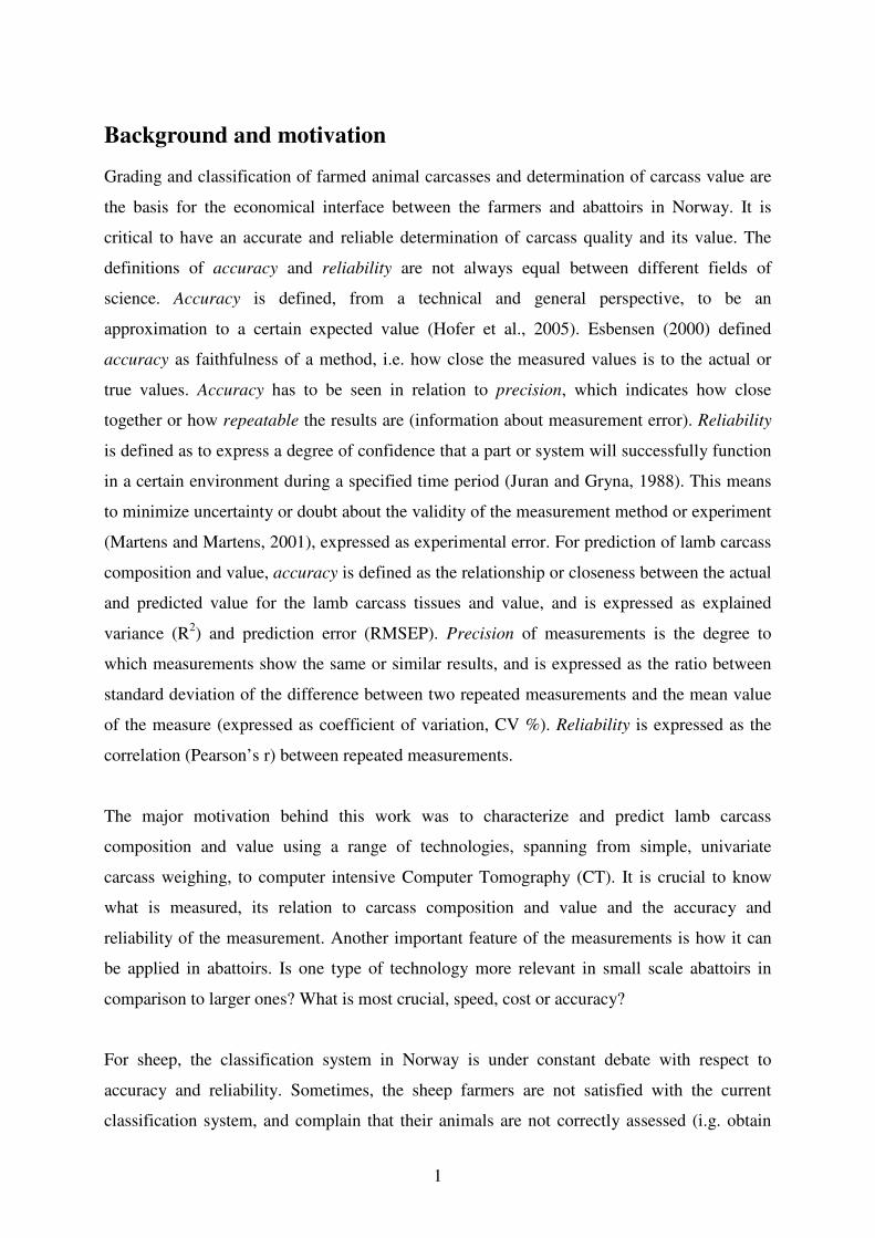
conformation across the entire carcass. Linear shape and size measurements of conformation

from the unpublished Norwegian trial are shown in Figure 4 (from paper #5); utilizing the

convex and concave shapes on a carcass more objectively using i.e. rulers and measuring

tapes.

Figure 4. EUROP advanced carcass shape (white or gray L1-L4, R1 and F1-F2) and length / width (black) measurements based on the detailed rules laid down by the EU commission concerning the classification of ovine animals. In addition, carcass length from 1st anterior rib to carcass steel hook was measured (from paper #5).

Video image analysis (VIA)

Video image analysis (VIA) is a fast and automatic method to assess the shape, length and

color of carcass surfaces. The technology is based on objective and computed assessment of

carcass shapes, lengths and surface color from digital images captured by a charge-coupled

device (CCD) camera on-line (Fig. 5) (Hopkins et al., 2004; Newman, 1987; Stanford et al.,

1998; Swatland, 1995). In a comparison study, a video image analysis system developed by

Meat and Livestock Australia, VIAScan®, was compared to hot carcass weight (HCW) and

tissue depth at grading rule (GR) site (thickness over the 12th rib, 11 cm from the midline),

13

with respect to prediction of lean meat yield (Hopkins et al., 2004). A greater prediction

accuracy (R2=0.52) was achieved by the VIAScan® system compared to HCW and GR

(R2=0.41). The VIAScan® system offered a workable method for predicting lean meat yield

automatically. The video image device Lamb Vision System (LVS), accounted for 50-54% of

the observed variation in boxed carcass value, compared to traditional HCW based value

assessment which accounted for 25-33% of the variation in boxed carcass value (Brady et al.,

2003). The LVS assessed individual lamb carcass value more accurately than the traditional

HCW assessment. Interestingly, the LVS was found to be highly accurate with respect to

prediction of lamb fabrication yields, with a repeatability of 0.98 (Cunha et al., 2004). For

beef carcasses, it was found that VIA was equally accurate to the EUROP classification scores

plus HCW in predicting saleable and primal yield (Allen, 2003). In a Norwegian trial using

the E+V vision system VSS2000 for lamb carcasses, it was found that VSS2000 compared

well with EUROP conformation scores (Berg et al., 2001). The repeatability was higher for

VSS2000 compared to trained operators for EUROP scores. In EU member states, new

technologies presented for carcass classification must be approved according to EU

Commission standards (Commission Regulation (EC) No 1215/2003, 2003). An annex was

added to this regulation in 2003, setting conditions and minimum requirements for

authorisation of automated grading techniques for beef. This annex is also valid for lamb,

since the requirements are equal, in practice. These requirements are based on prediction of

EUROP grading or classification scores, and not weight or yield of meat and sub-primals. The

prediction of EUROP scores will be a prediction of a prediction, since EUROP is a method

for predicting market value. This cannot be considered an optimal solution in practice, and

raises the following question: What is the actual reference; EUROP scores or weight / yield?

The common practice in some countries have been to meet the requirements of the EU

commission for EUROP grading and classification towards farmers, and use the VIA systems

for predicting saleable meat yield within the company for process control. The main concern

from the EU Commission is that saleable meat yield is difficult to standardize and to

harmonize between the member states. For now, it seems like harmonization is favoured in

contrast to higher accuracy and estimation of yields by using VIA and other automatic

technologies. In Norway, the VSS2000 system has not yet passed the requirements for

prediction of EUROP scores. The use of the system for on-line prediction of primal cut and

saleable meat yield has not yet been fully utilized in Norway, however, the system have

shown to be very accurate (Berg et al., 2001). The trend in Europe seems to shift towards the

same marketing initiatives involving payment of farmers based directly on the assessment of

14

carcass value by VIA in New Zealand (Jopson et al., 2005). In New Zealand, one of the

largest meat processors has recently installed VIA systems in all of its sheep plants, and the

other meat companies are working on similar systems (Jopson et al., 2005). Despite VIA’s

recent popularity in the meat industry, the main future challenge for VIA systems, however, is

to introduce a new reference or payment system based on saleable meat yield or the value of

the carcass directly. The experience so far has been that this is a rather slow process where the

changes will be gradual.

Figure 5. Video Image Analysis. CCD image of lamb carcass.

Visible light reflectance probing

Visible light reflectance probing is a spectroscopic method which utilizes the reflectance of

visible light from different types of tissues. The probe is inserted into i.e. the loin of a carcass,

and a profile of the loin, from back-fat to the body cavity (costa) is measured (Fig. 6). The

probe is an evolution of the manual caliper used to perform length and width measurements.

The data generated for industrial use from the probe are fat and muscle thickness. The tip of

the probe contains a light-emitting diode followed by a light detection device (Berg et al.,

1997). Muscle and fat tissue reflects the light differently, and this difference is used to

measure muscle and fat depth at the probe site. Optical probes are considered to be invasive,

although penetration damage is minimal (Swatland et al., 1994). Optical probing is currently

used in Norway and other European countries for grading of pig carcasses by measuring

backfat and m. longissimus thickness. Recent advances of the probe provide the color and

level of marbling in the muscle. The color can be related to meat quality attributes, and is

currently used in Norway to identify Pale Soft Exudative (PSE) meat on pigs. However, it has

recently been questioned in the Norwegian pork meat industry how increased marbling (intra

15

muscular fat) impacts the measurements. This concern may be excessive, since the “noise”

from marbling can be modeled statistically and may not compromise the accuracy of

measurements. In New Zealand and Australia, lamb and sheep carcasses are graded using

grading probes, measurements of back-fat in the same fashion as pig carcasses in Europe.

Probing by using GR or other back-fat measures is considered to be more robust and accurate

compared to visual appraisal using the EUROP system (Kempster et al., 1986a). Probe

measurement of backfat thickness between the 12th and 13th rib provided a superior method

compared to visual assessment for prediction of lean content in lamb carcasses (Jones et al.,

1992). In Europe (including Norway), there has been a major concern using probing for sheep

and cattle, due to large variation in breeds and crossbreeds, and damaged subcutaneous fat

cover during slaughter and hide-pulling (Augustini et al., 1994; Kirton, 1989). In Iceland,

probe measurements (ICEMEAT probe) of backfat and side thickness has proven to be

successful (Einarsdottir, 1998), probably due to a very homogenous population of sheep

(Icelandic sheep breed). In Iceland and New Zealand, no major concerns have been raised

concerning damaged subcutaneous fat during slaughter (Kirton, 1989), however there are

some concerns due to positioning and operation of the probe at high chain speed.

Figure 6. Visible light reflectance probe (Hennessy Grading Probe®). Measurement of lamb side and backfat thickness assessed by the author J. Kongsro. Reflectance profile from Hennessy Grading Probe®, from backfat to body cavity. Reflectance peaks (white) at back-fat and costa (high fat).

The repeatability of probe measurements is highly dependent on the operator of the equipment

(Olsen et al., 2007). Robotics or support frames can increase the repeatability of

measurements by visible light reflectance probing (Swatland et al., 1994). The cost of

equipment is also an issue; however, the price of visible reflectance probes is relatively low.

Robotics and support frames will also increase cost; however, increased repeatability will pay

off over time. Stanford et al. (1998) found that the increased accuracy of optical probing

compared to manual GR measurements of back-fat, was likely due to improvements in the

accuracy of prediction of carcass composition of cold as compared to warm carcasses. The

reason for the improvement in accuracy and repeatability of cold vs. warm carcasses may be

16

errors caused by fat bubbles in subcutaneous fat when the hide is removed from warm

carcasses. During chilling of carcasses, the fat bubbles are reduced significantly and the

subcutaneous fat layer obtains a more even shape and thickness. The effect of fat bubbling on

subjective appraisal or VIA has, however, not been documented. Information on meat color

and quality from GP is an additional advantage. When measuring meat color, time post

mortem is of great importance. Measurements of color 24 hours post mortem and 7 days post

mortem are different (Linares et al., 2007). The accuracy of probes can probably be improved

by increasing the number of measuring sites, sampling from several anatomical positions

along the carcass. However, the penetration damage may increase by adding probing sites,

and may be too invasive in practice. The operation at high chain speed may also be an issue

when introducing several measuring sites.

Total Body Electrical Conductivity (TOBEC) and Bioelectrical Impedance (BIA)

Total Body Electrical Conductivity (TOBEC) and Bioelectrical Impedance (BIA) are methods

which utilize the transfer of an electrical current through biological material like a lamb

carcass. Lean tissue is much more conductive than fat and bone tissue due to the high

concentration of water and electrolytes in the tissue (Stanford et al., 1998). A fat lamb carcass

should impede the transmission of electrical current to a larger extent than a lean lamb (Berg

et al., 1996). Using this difference between tissues in electrical conductivity or impedance, the

carcass composition can be predicted. Berg et al. (1996) also found that individual electronic

methodologies tested in their study were moderate predictors of proportional carcass lean

(Berg et al., 1996). Another study reported that the impedance method is not suitable for the

prediction of carcass composition, neither in lambs of similar weight nor in heterogeneous

animals (Altmann et al., 2005). For TOBEC, is was found that the research approach using

electromagnetic scanning was not a reliable tool for predicting body composition of live

lambs (Wishmeyer et al., 1996). Overall, it seems that methods using transfer of an electrical

current through a lamb carcass need to be further developed to achieve higher accuracy and

reliability.

Computer Tomography (CT)

Computer Tomography was introduced for medical diagnostics in the 1970’s (Hounsfield,

1973), for which G. N. Hounsfield and A.M. Cormack received the Nobel Price in Medicine

in 1979. The method is computer intensive, and the principle is based on X-ray attenuation

through an object, where an X-ray source and detectors rotate 360o around the object (Fig. 7).

17

For sheep, CT has primarily been used for selection of breeding traits (Kvame, 2005) and

prediction of lamb carcass tissue weights (Junkuszew and Ringdorfer, 2005; Lambe et al.,

2003).

Figure 7. Left: Computer Tomography (CT) scanner. Lamb carcass subject for assessment. Right: CT Tomogram Image. Image sampled from mid-part of carcass (11th rib).

X-ray images are generated during rotation of the X-ray tube, and data recovered from the X-

ray detectors are reconstructed by a computer to form a tomogram or CT image of the entire

object, both internally and externally (Fig. 7). A set of CT images from a set of trans-sectional

images or spiral scanning can be used to generate 3D images or volumes of the object

subjected for study. Different tissues produce different degrees of X-ray attenuation,

reflecting their density, thickness and atomic number (Harvey and Blomley, 2005). Lower

density tissues will appear more transparent than higher density tissues to X-rays. Air is

transparent to X-rays, and will appear black, while bone, due to its high mineral content, is

not very transparent, and appears white in CT images. In radiographic terms, the transparency

of X-rays is often called radiodensity, and is quantified in Hounsfield Units (HU), where the

X-ray attenuation of distilled water is used as a Hounsfield scale reference (HU=0). The

images generated from CT can be analyzed using the HU value of each pixel. CT images can

be organized according to spectroscopic profiles using the histogram of pixels, where the

intensity of pixels can be visualized according to the respective CT value (HU) (Fig. 8). Fat

tissue has a lower density compared to muscle tissue, and much lower density than bone

tissue. To get a better separation of tissues with respect to radiodensity, contrasting agents can

be added via feeding pre-slaughter or via blood vessels (i.e. for segmentation of internal

organs using iodine).

18

-200 -100 0 100 2000

2000

4000

6000

8000

10000

12000

CT value (HU)

Fre

qu

en

cy p

ixels

Figure 8. CT histogram pixels from 120 lambs (left) (samples from paper III). Soft tissue region from HU value -120 to 120. The first, smaller peak was identified as fat tissue, the second, larger peak identified as muscle tissue (right).

The CT histograms can be decomposed using two strategies: (1) utilize a priori knowledge or

windowing of CT values (Kalender, 2005) reflecting the CT values of fat, muscle and bone

tissue, or (2) through calibration of CT histograms against a known reference such as

commercial or full dissection (Dobrowolski et al., 2004). If the a priori knowledge is robust

and globally valid for new samples, the computation is both fast and efficient. If there are

differences in CT value windows or radiodensity for the same tissue (i.e. muscle) between and

within populations of lambs, the predictions will be less accurate using windowing. A pixel

will represent the mean value of the area covered by the pixel, and the pixel may sometimes

(i.e. border pixels between two types of tissues) represent an average of two tissues, making

discrimination between the tissues difficult. This mixed pixel distribution is called the partial

volume effect (Lim et al., 2006). It is therefore of great importance to perform calibrations by

using representative samples of the actual carcass population which CT is meant to predict.

Using the calibration strategy, the CT values are calibrated against real data sampled from the

actual population you want to model. The calibration is performed using the spectroscopic

approach, where the CT histogram is treated as a spectrum, and can be modeled using

multivariate calibration. Regression coefficients can be estimated from calibration, and can be

used as window levels or models for further prediction of carcass tissues. The disadvantage of

calibration, is that the reference method used (dissection) is often inaccurate and have poor

repeatability due to butcher or operator error, as shown for pig carcass dissection (Nissen et

al., 2006).

19

By using stereological methods such as the Cavalieri principle (Russ, 2002), unbiased

estimates of the tissue volumes can be obtained (Fig. 9). The CT images are organized in

sections based on the equipment settings and method, and the total volume of the segmented

tissue will be the area of tissue in the CT images, multiplied by the section distance.

Dissection seemed to be a choice between accuracy and number of samples; full tissue

separation vs. commercial dissection. CT can offer a combination of both, providing a high

number of “low-cost” estimates of full tissue separation. Dissection using CT is sometimes

nicknamed “virtual dissection”, where live animals or carcasses can be dissected in virtual

space using a computer. For industrial on-line use, it has been stated that CT would be too

slow, even if it is cost-effective (Stanford et al., 1998). Advances in CT technology since

1998, has proven that CT can operate during high speed in hospital environments. Single

scans of selected anatomical sites can in theory be obtained in 0.8 seconds (scan time;

protocol). High-speed dual-source computed tomography scanning (DSCT) of human hearts

have been performed with mean scan times of 8.58 seconds (Weustink et al., 2007). CT

scanners may be able to predict lamb carcass composition on-line at chain speed; it is just a

matter of designing a CT scanner for abattoir environments.

Figure 9. Cavalieri estimation and visualization of lamb carcass side using CT (left). Fat (yellow), muscle (red) and bone (light gray) segmented using windows presented by (Kvame et al., 2004).

20

Summary of methods and economical considerations

Table 2. Summary of different methods or technologies (systems) for prediction of lamb carcass tissues presented, with respect to explained variance and prediction error. System (independent) Tissue reference

(dependent)

Explained

variance

RSD

RMSE Reference

Live weight Muscle (kg) R2 = 0.96 (Teixeira et al., 2006) HCW Muscle (g) R2 = 0.92 RSD = 69.94 (Diaz et al., 2004) Leg fat (%) Carcass fat (%) R = 0.93 RSD = 1.55 (Kirton and Barton,

1962) Loin fat (%) Carcass fat (%) R = 0.97 RSD = 1.07 (Kirton and Barton,

1962) Specific gravity (hind saddle)

Carcass fat trim % R2 = 0.51 (Adams et al., 1970)

Linear carcass measures Total dissected lean (%) R2 = 0.72 RMSE = 2.55 (Berg et al., 1997) Linear carcass measures Total dissected lean (kg) R2 = 0.86 RMSE = 0.78 (Berg et al., 1997) Linear carcass measures Muscle (%) R2 = 0.63 RSD = 1.55 (Diaz et al., 2004) Linear carcass measures Fat (%) R2 = 0.84 RSD = 1.83 (Diaz et al., 2004) EUROP classification Fat (%) R2 = 0.57 RSD = 2.35 (Einarsdottir, 1998) EUROP classification Lean meat (%) R2 = 0.23 RSD = 2.54 (Einarsdottir, 1998) GR Carcass fat (%) R2 = 0.57 -

0.58 RSD = 2.97 (Kirton et al., 1995)

Ultrasound Total dissected lean (%) R2 = 0.26 RMSE = 4.46 (Berg et al., 1996) Ultrasound Total dissected lean (kg) R2 = 0.54 RMSE = 1.31 (Berg et al., 1996) Ultrasound Fat (%) R2 = 0.06 -

0.41 (Olesen and Husabø,

1992) HC Fat (%) R2 = 0.73 RSD = 2.06 (Einarsdottir, 1998) ICEMEAT Lean meat (%) R2 = 0.28 RSD = 2.53 (Einarsdottir, 1998) HC + EUROP Fat (%) R2 = 0.80 RSD = 1.80 (Einarsdottir, 1998) HC + EUROP Lean meat (%) R2 = 0.38 RSD = 2.46 (Einarsdottir, 1998) Electronic probe Carcass fat (%) R2 = 0.47 -

0.58 RSD = 2.99 - 3.48

(Kirton et al., 1995)

BIA Fat-free soft tissue (kg) R2 = 0.94 RSD = 0.43 (Jenkins et al., 1988) BIA + linear carcass measures

Fat-free soft tissue (kg) R2 = 0.96 RSD = 0.34 (Jenkins et al., 1988)

HCW + VIA (color + shape)

Saleable meat yield (%) R2 = 0.71 RSD = 1.43 (Stanford et al., 1998)

VIA + HCW Saleable meat yield (%) R2 = 0.64 RMSE = 3.30 (Brady et al., 2003) TOBEC Dissected lean (%) R2 = 0.62 RMSE = 2.97 (Berg et al., 1997) TOBEC Dissected lean (kg) R2 = 0.83 RMSE = 0.85 (Berg et al., 1997) CT Primal weight (kg) R2 = 0.85 -

0.98 RSD = 0.02 - 0.37

(Kvame et al., 2004)

CT Primal lean (kg) R2 = 0.80 - 0.98

RSD = 0.01 - 0.32

(Kvame et al., 2004)

CT Primal fat, subcutaneous and intermuscular (kg)

R2 = 0.82 - 0.98

RSD = 0.004 - 0.09

(Kvame et al., 2004)

CT Fat (kg) R2 = 0.80 - 0.84

(Junkuszew and Ringdorfer, 2005)

CT Muscle (kg) R2 = 0.63 - 0.65

(Junkuszew and Ringdorfer, 2005)

BIA = Bioelectrical impedance CT = Computer Tomgraphy GR = fat thickness, grading rule site (mm) HC = Icelandic Manual GR meter (hot carcass) HCW = hot carcass weight ICEMEAT = ICEMEAT GR probe (cold carcass)

Rack = lamb loin with ribs RMSE = Root Mean Square Error RSD = Residual Standard Deviation SE = Standard Error TOBEC = total body electrical conductivity VIA = Video Image Analysis

21

The usefulness of different measurements or methods from previous studies was compared in

table 2, with respect to explained variance (R2) and residual standard deviation (RSD) or root

mean square error (RMSE), when available. The table spans from live or carcass weight,

subjective appraisal and linear measurements, electronic probing and bioelectrical impedance,

and finally computer tomography (CT).

The usefulness for tissue composition in weights (kg) seems to be more accurate than those

for tissue proportion in percentage. For practical purposes, the most accurate solution seem to

be to estimate the carcass tissue in weight, then, an estimate of the proportion can be obtained

as a proportion of carcass weight; tissue (kg) * carcass weight-1 (kg). The results in Table 2

show that live or carcass weight is a very good single predictor of both fat and muscle weight

in kg. The best measuring systems in Table 2 with respect to explained variance, RSD or

RMSE seem to be Computer Tomography (CT). The authors used single scans from selected

anatomical sites (Junkuszew and Ringdorfer, 2005) or sequential scanning using 50 mm

section distances, with an average of 18 images per animal (Kvame et al., 2004). By using

denser scans with smaller section distances or spiral scanning, the accuracy may be improved.

Results from spiral scanning of pig carcasses have shown that the predictions were very good

and provided a fast volumetric scanning method of the entire carcass (Dobrowolski et al.,

2004; Fuchs et al., 2003; Kalender, 1994; Romvari et al., 2006). Using tissue proportions

obtained from primals have shown to be very well correlated with carcass tissue proportion

(Kirton and Barton, 1962). However, primal dissection used as predictor of carcass

composition is a laborious process, which has little relevance in a practical setting. The error

of determining the tissue reference (i.e. by dissection) has not been quantified in any of the

previous studies. A significant error in the reference will inevitably have an effect of the

precision of the measuring method. This can be solved by repeated measurements, i.e.

estimating paired differences between repeated measurements, depending on how costly or

time consuming the measurements are (Esbensen, 2000).

22

Multivariate calibration

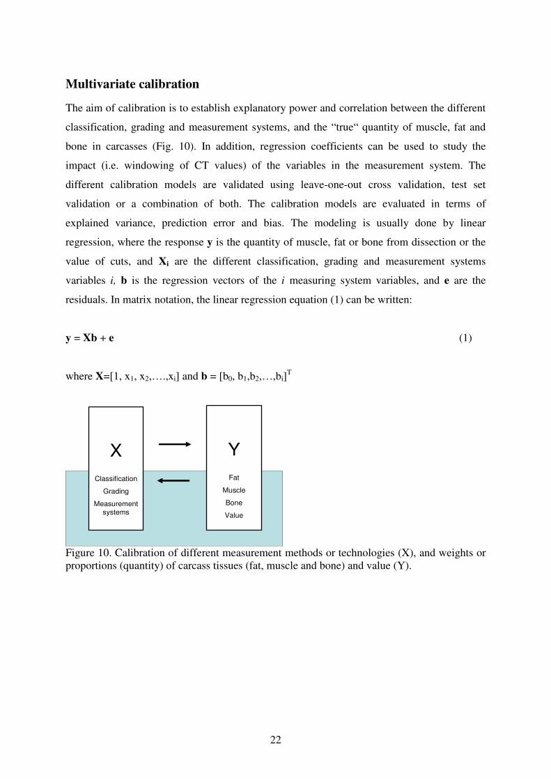
The aim of calibration is to establish explanatory power and correlation between the different

classification, grading and measurement systems, and the “true“ quantity of muscle, fat and

bone in carcasses (Fig. 10). In addition, regression coefficients can be used to study the

impact (i.e. windowing of CT values) of the variables in the measurement system. The

different calibration models are validated using leave-one-out cross validation, test set

validation or a combination of both. The calibration models are evaluated in terms of

explained variance, prediction error and bias. The modeling is usually done by linear

regression, where the response y is the quantity of muscle, fat or bone from dissection or the

value of cuts, and Xi are the different classification, grading and measurement systems

variables i, b is the regression vectors of the i measuring system variables, and e are the

residuals. In matrix notation, the linear regression equation (1) can be written:

y = Xb + e (1)

where X=[1, x1, x2,….,xi] and b = [b0, b1,b2,…,bi]T

X

Classification

Grading

Measurement

systems

Y

Fat

Muscle

Bone

Value

Figure 10. Calibration of different measurement methods or technologies (X), and weights or proportions (quantity) of carcass tissues (fat, muscle and bone) and value (Y).

23

Table 3. Classification of data by their tensorial properties, and typical methods for data analysis (Escandar et al., 2006). Instrument data examples, regression method and second order advantage. Classification Order of

data

Sample

data set

Instrument

data

Typical

method

Second

order

advantage

Univariate Zeroth-order One-way - Fat thickness - EUROP fat score

OLSR No

Multivariate First-order Two-way - Set of fat thickness (GP probing) - CT histogram

PCR, PLSR No

Higher-order unfolded to first-order

Two-way CT histogram

Unfold PCR Unfold PLSR

No

Second-order Three-way CT histogram

PARAFAC NPLSR

Yes

CT = Computer Tomography

GP = visible light reflectance probing

NPLSR = N-way PLSR

OLSR = Ordinary Least Squares Regression

PARAFAC = Parallel Factor Analysis

PCR = Principal Component Regression

PLSR = Partial Least Squares Regression

Many instrumental measurements produce one, two or multidimensional arrays of data. The

different dimensions of data is called the order of data (Escandar et al., 2006). The different

dimensions of data produced by classification, grading or other measurement are seen as the

components of a first-, second- or nth-order tensor, respectively (Sanchez and Kowalski,

1987). The univariate case or zeroth-order of data can be exemplified by fat thickness

measured at a singe site as a single vector x and total fat from a carcass in kg as a y. This is

handled by Ordinary Least Squares regression (OLSR) (Tab. 3). Univariate calibration or

modeling using estimates to predict the quantity of carcass tissues are sometimes called direct

estimation. Another example of univariate calibration can be tissue estimates from CT

scanning using windowing. In this case, single estimates (vector x) from CT scanning is

calibrated against a cutting reference y. When introducing a set of measurement variables

such as EUROP conformation and fat classes, carcass weight and several fat thicknesses

probed by GP, we enter the multivariate domain with several variables in X. This is best

handled by multivariate calibration methods such as Principal Component Regression (PCR)

24

or Partial Least Square Regression (PLSR). The original sets of sampled responses within

these variables are transformed into scores by latent variable selection, and regression is

performed on these scores. Higher order data has recently been applied to a number of

different fields within analytical chemistry and food science (Andersen and Bro, 2003; Bro,

1996; Escandar et al., 2006; Huang et al., 2003). These data are provided by i.e. sampling

using multi-component instruments and cross-section images from CT. The data are

recognized by each sample providing a data array (multi-way) instead of a vector (2-way).

This multi-way data array can be handled in two different ways; either by unfolding the

higher order (I * K * L) data set to a first-order (two-way) data set by rearranging the data

across a higher order mode (IK * L) (Chiang et al., 2006). There are several advantages of

keeping the higher order data structure in the previous example, called the second-order

advantage. The second-order advantage makes it possible to utilize the multi-way structure,

like in the previous example, and extracting valuable information concerning the higher order

structure, i.e. cross section from CT images.

One of the requirements of linear regression is that the variables X should preferably be

independent or orthogonal (Martens and Martens, 2001). In measuring systems, the variables

are often correlated, and calibration and prediction may suffer from collinearity when using

OLSR. OLSR has a number of assumption, for example that the errors are independently

distributed and that the independent variables are not to strongly correlated or collinear

(Esbensen, 2000; Martens and Martens, 2001). When collinearity is high, it is almost

impossible to obtain reliable estimates of regression coefficients. It does not affect the ability

of the regression to predict the response; however, the estimates or contribution of the

individual regression coefficients bi becomes unstable. The main purpose of regression is to

seek the largest explanation of variance in y as a function of X. The obvious solution seems to

be removal of one or more of the correlated variables in X. Instead of looking at collinearity

as a problem, some multivariate calibration methods utilize the correlation between variables,

and construct a set of latent variables which are orthogonal (independent). The latent variables

are estimated as linear functions of both original input variables and the observations, and is

often called bilinear modeling (BLM) (Esbensen, 2000; Martens and Martens, 2001), as

shown in Figure 11. Principal Component Analysis (PCA) or Principal Component

Regression (PCR) and Partial Least Square Regression (PLSR) are some bilinear methods

which handle collinearity and construct a set of orthogonal latent variables called principal

components for further calibration. The goal of PCR and PLSR is to fit as much variation as

25

possible using as few PCs possible (Martens and Martens, 2001). The first latent variable or

PC explains the largest amount of variation, the 2nd the second largest, and so on. The original

variables are projected down to the PCs space, and are called loadings. The measurements or

information carried by the original variables are also compressed and projected down on the

PC space, and are called scores. Each sample has a score along each PC (Esbensen, 2000).

For each PC, we have loadings and scores which reflect the compression of the original data

structure with samples and variables (Fig. 11). The number of latent variables is always

smaller than the original data set; especially for spectroscopic studies, where the number of

variables (i.e. wavelengths) is very large. PCR focus on obtaining PCs from the X data array,

followed by regression of Y using the scores obtained from the PC. For PLSR, the modeling

of PCs is done by seeking the largest covariance between X and y or ensuring y-relevant PCs

from X (Martens and Martens, 2001). The result is that the PLSR models are simpler and

more compact models, and in most cases uses fewer PCs compared to PCR.

X t

l

=

Figure 11. Bilinear modeling. Latent variable decomposition of a data set X. Scores (t) and loadings (l).

The performance of a multivariate calibration model is quantified by validation. The purpose

of validation is two-fold (Esbensen, 2000): (1) to make sure that the calibration model will

work in the future, on new data sets and (2) to find the optimal dimensionality of the model to

avoid under- or overfitting. The overall aim of validation is to obtain the lowest prediction

error possible using the optimal dimensionality of the model. The calibration modeling error

is defined as the Root Mean Square Error of Cross Validation (RMSECV). The cross-

validated model is tested using a separate test set, and the prediction error is found using the

Root Mean Square Error of Prediction (RMSEP).

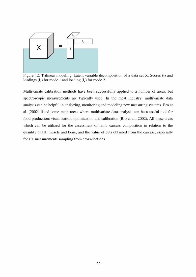
The bilinear modeling handles first-order data structures (samples*variables). For higher-

order data structures, i.e. second-order or three way data matrices, two original input spaces of

26

variables and the observations are modeled, and this is often called trilinear modeling. A set

of scores and two sets of loadings are estimated from the trilinear modeling (Fig 12). NPLSR

is PLSR for multi-way or higher order data, where trilinear modeling estimates a set of scores

and n set of loadings, where n is larger than 1. PARAFAC or Parallel Factor Analysis was

introduced in two parallel papers by (Carroll and Chang, 1970; Harshman, 1970) for

psychometric studies, and has been further developed for Chemometrics by Bro (Bro, 1997).

PARAFAC is a generalization of PCA into higher order data arrays, but is somewhat different

from the bilinear PCA (Bro, 1997). PARAFAC yields n number of loadings when there are n

modes or dimensions in the data, and often the first mode is named scores and represent the

information in samples or objects (Rinnan, 2004). The decomposition of data using

PARAFAC differs from PCA by providing unique solutions (Bro, 1997), calculating all

components simultaneously, different from PCA which calculates one component at a time.

The components in PARAFAC will represent the unique solution in X, while PCA will seek

the largest covariance in X. If the optimal number of components is selected, and the data is

trilinear or higher order in nature and a global optimum is achieved, PARAFAC is a robust

and strong tool for decomposition and modeling of multi-way data. While PCR, PLS and N-

PLS for multi-way data require reference samples for modeling (y), the uniqueness of

PARAFAC makes it able to estimate the true underlying profiles in the multi-way data set

(Khayamian, 2007). The optimal number of components can be found by different validation

techniques, like core consistency and split-half analysis (Trevisan and Poppi, 2003). If the

PARAFAC model is correct, then it is expected that the superdiagonal elements will be close

to one and the off-diagonal elements close to zero, and core consistency is achieved (Trevisan

and Poppi, 2003). In an optimal PARAFAC model, the core consistency should be as close to

100% as possible (Bro and Kiers, 2003). Another validation tool is split-half analysis. The

idea of this analysis is to divide the data set into two halves and make a PARAFAC model on

both halves. Due to the uniqueness of the PARAFAC model, one will obtain the same result

on both data sets, if the correct number of components is chosen (Christensen et al., 2005).

27

X t

l1

l2

=

Figure 12. Trilinear modeling. Latent variable decomposition of a data set X. Scores (t) and loadings (l1) for mode 1 and loading (l2) for mode 2.

Multivariate calibration methods have been successfully applied to a number of areas, but

spectroscopic measurements are typically used. In the meat industry, multivariate data

analysis can be helpful in analyzing, monitoring and modeling new measuring systems. Bro et

al. (2002) listed some main areas where multivariate data analysis can be a useful tool for

food production: visualization, optimization and calibration (Bro et al., 2002). All these areas

which can be utilized for the assessment of lamb carcass composition in relation to the

quantity of fat, muscle and bone, and the value of cuts obtained from the carcass, especially

for CT measurements sampling from cross-sections.

28

Main results of papers I-V and future perspectives.

This thesis focuses on reliable prediction and determination of lamb carcass composition

using different methods or techniques.

The objective of Paper I was to study the repeatability and accuracy of the EUROP

classification system applied in Norway. The assessors were highly reliable, achieving high

correlation between repeated measurements and between assessors. There were some

differences between abattoir operators and EU commission assessors, but these differences

were within limits accepted by the EU commission. The EUROP prediction of lean meat

percentage was poor, achieving relatively high prediction error and low explained variance.

The prediction of bone and fat percentage was somewhat better, especially for fat. This

showed that EUROP does not predict lean meat in carcasses very well, but is somewhat

accetable for prediction of fat.

The precision and reliability of lamb carcass dissection as the reference method for lamb

carcass classification and grading has never been quantified. In paper II, an estimate of the

reliability and precision of the reference butcher panel used for calibration of lamb carcass

classification and grading in Norway was obtained from a sample set of Norwegian lambs.

The goal was to develop a methodical framework to study the accuracy of lamb carcass

dissection in Norway; describe and obtain estimates of the precision and reliability of the

reference dissection in Norway for calibration of lamb carcass classification. The overall

precision and reliability was acceptable (reliability > 0.80) for carcass composition traits,

however, the results for sub-primal yield and composition were somewhat poorer. The sub-

primal breast seemed to be difficult for the butchers to dissect, and needs special attention

when setting up a dissection of lamb carcasses.

In paper III, the objective was to find the best prediction model for carcass soft tissues (fat

and muscle) using Computer Tomography (CT). The digital image data from CT scanning

was organized according to histograms of CT value and anatomical direction, yielding a

multi-way data array. Two strategies of modeling were tested. The first, direct estimation was

based on a priori thresholds of fat and muscle tissue in CT images or scores from PARAFAC

modeling of the multi-way data array. The second strategy was based on multivariate

calibration using 2-way PLS or n-way NPLS against a commercial dissection reference. The

29

results showed that multivariate calibration using NPLS gave the best results for fat and

muscle tissue with respect to prediction error (RMSEP). There were some biases between

measured (dissection) and predicted (CT) fat and muscle, and bias corrections proved to be

advantageous for the models.

In paper IV, the objectives were: (1) to obtain estimates of precision and reliability using

virtual dissection by CT scanning of lamb carcass, and (2) to test different equidistances or

section distances using sequential CT scanning with respect to correlation between manual

commercial and virtual dissection. The precision and reliability of virtual dissection was

higher (reliability > 0.95) compared to manual commercial dissection in paper II. Increasing

section distances gave poorer accuracy, which is an effect of poor modeling of irregular 3D

structures (i.e. bone cartilage) in carcasses. There were some biases between manual and

virtual dissection, especially for bone and muscle. This may be a combination of butcher error

and modeling by sequential scanning. Spiral scanning may solve the bias problem and

modeling of 3D structures, and may prove CT to be a more accurate reference compared to

manual commercial dissection.

In paper V, a number of different technologies for measuring carcass soft tissues (fat and

muscle) and carcass value were tested with respect to accuracy and prediction. Four

technologies were tested on the same data set, spanning from manual EUROP classification to

Computer Tomography (CT) scanning of carcasses. CT yielded the highest overall accuracy

and most unbiased predictions, both for fat and muscle tissue. Currently, CT may be too slow

and expensive for on-line, however, recent developments of CT scanners may operate at chain

speed in the near future. The chain speed at Norwegian abattoirs during lamb slaughter season

is approx. 300-400 animals per hour. The most practical solution at the time for prediction of

carcass soft tissues and value, seem to be optical probing of carcass side thickness calibrated

against a CT virtual dissection reference.

The calculation of costs when introducing new measuring systems for lamb carcass

composition needs further attention.

� Does the increased accuracy and reliability of an alternative or new measuring system,

relate to the running, development and training costs?

� Are some types of measuring systems more relevant for larger abattoirs than for

smaller ones?

30

In this work, different technologies for prediction of carcass composition and value have been

tested, and current and alternative reference methods used for prediction have been evaluated

with respect to accuracy and reliability. The speed and cost of maintaining the current

EUROP classification system must be compared with the development costs and maintenance

of new technologies. A cost-benefit study beyond this work will determine the future

developments of technologies for prediction of carcass composition and value. In addition,

CT images, once available may provide many other relevant data in slaughter houses:

intramuscular fat, abnormal water to protein ratios of lean meat. Palatability traits such as

tenderness, juiciness etc., have not been addressed in this thesis. These traits must be

considered in future work in development of new systems for carcass evaluation. CT scanning

has proven throughout this work as the most accurate and reliable tool for prediction of

carcass composition. Spiral scanning of carcasses was not applied in this work; however it

may prove to be the best solution, covering variation in complex 3D structures (i.e. bone

cartilage) in carcasses. For future work using CT scanning, spiral scanning is therefore highly

recommended. Whether the methods or technologies presented in this thesis are dependent on

size of abattoirs or plants may be discussed, but it seems obvious that smaller plants with a

smaller turnover of carcasses and meat will not be able to benefit as much as larger plants, i.e.

fixed costs of expensive equipment. The size of plants is a major concern when trying to

harmonize the classification or grading methods between and within countries or regions. This

emphasises the need of an objective and reliable reference, in which the plants can use as a

measure. New methods or technologies needs to be measured and validated against this

reference, in order to obtain solid risk assessment, both in terms of accuracy and cost.

During this work, an application using CT as a reference method for carcass composition and

value has shown to be more accurate, cheaper and reliable compared to manual dissection

performed by butchers. In terms of measuring systems, smaller plants can to a large degree

utilize carcass weight or simple linear measures, and still obtain an accuracy close (or

sometimes better) to more computer-intensive systems like VIA and BIA. When investing in

new technology for prediction of lamb carcass composition and value; the easiest solution is

most often the best one, and it all depends on the reference method used for prediction.

31

References

Adams, N. J., Z. L. Carpente, and C. W. Spaeth. 1970. Estimation of Lamb Carcass Composition by Use of Specific Gravity Measurements. J. Anim Sci. 31:1081-1088.

Allen, P. 2003. Beef Carcass Grading in Europe and U.S.A. - The Prospects for Using VIA Systems. Page 96 in Proceedings. ICoMST, Campinas, Brazil.

Altmann, M., U. Pliquett, R. Suess, and E. von Borell. 2005. Prediction of carcass composition by impedance spectroscopy in lambs of similar weight. Meat Science 70:319-327.

Andersen, C. M. and R. Bro. 2003. Practical aspects of PARAFAC modeling of fluorescence excitation-emission data. Journal of Chemometrics 17:200-215.

Augustini, C., A. Dobrowolski, and F. Heining. 1994. Objective Evaluation of Bovine Carcasses. Fleischwirtschaft 74:1059.

Barton, R. A. and A. H. Kirton. 1956. Determination of fat in mutton carcasses by measurement of specific gravity. Nature 178:920.

Berg, E. P., J. C. Forrest, D. L. Thomas, N. Nusbaum, and R. G. Kauffman. 1994. Electromagnetic Scanning to Predict Lamb Carcass Composition. J. Anim Sci. 72:1728-1736.

Berg, E. P., M. K. Neary, J. C. Forrest, D. L. Thomas, and R. G. Kauffman. 1996. Assessment of lamb carcass composition from live animal measurement of bioelectrical impedance or ultrasonic tissue depths. J. Anim Sci. 74:2672-2678.

Berg, E. P., M. K. Neary, J. C. Forrest, D. L. Thomas, and R. G. Kauffman. 1997. Evaluation of electronic technology to assess lamb carcass composition. J. Anim Sci. 75:2433-2444.

Berg, P., H. Eger, J. S. Løkting, and M. Røe. 2001. Automatic grading of sheep by vision. Page 24 in Proceedings. 47th ICoMST, Krakow, Poland.

Brady, A. S., K. E. Belk, S. B. LeValley, N. L. Dalsted, J. A. Scanga, J. D. Tatum, and G. C. Smith. 2003. An evaluation of the lamb vision system as a predictor of lamb carcass red meat yield percentage. J. Anim Sci. 81:1488-1498.

Bro, R. 1996. Multi-Way Calibration. Multi-Linear PLS. Journal of Chemometrics 10:47-62.

Bro, R. 1997. PARAFAC. Tutorial and applications. Chemometrics and Intelligent Laboratory Systems 38:149-171.

Bro, R. and H. A. L. Kiers. 2003. A new efficient method for determing the number of components in PARAFAC models. Journal of Chemometrics 17:274-286.

Bro, R., F. van den Berg, A. Thybo, C. M. Andersen, B. M. Jorgensen, and H. Andersen. 2002. Multivariate data analysis as a tool in advanced quality monitoring in the food production chain. Trends in Food Science & Technology 13:235-244.

32

Carroll, J. D. and J.-J. Chang. 1970. Analysis of Individual Differences in Multidimensional scaling via an N-way generalization of "Eckart-Young" Decomposition. Psychometrika 35:283-319.

Chandraratne, M. R., D. Kulasiri, C. Frampton, S. Samarasinghe, and R. Bickerstaffe. 2006. Prediction of lamb carcass grades using features extracted from lamb chop images. Journal of Food Engineering 74:116-124.

Chiang, L. H., R. Leardi, R. J. Pell, and M. B. Seasholtz. 2006. Industrial experiences with multivariate statistical analysis of batch process data. Chemometrics and Intelligent Laboratory Systems 81:109-119.

Christensen, J., E. M. Becker, and C. S. Frederiksen. 2005. Fluorescence spectroscopy and PARAFAC in the analysis of yogurt. Chemometrics and Intelligent Laboratory Systems 75:201-208.

Colomer-Rocher, F., J. J. Bass, and D. L. Jonhson. 1980. Beef carcass conformation and some relationships with carcass composition and muscle dimension. J. Agric. Sci. (Camb. ) 94:697.

Commission Regulation (EC) No 1215/2003. 2003. Commission Regulation (EC) No 1215/2003 of 7 July 2003 amending Regulation (EEC) No 344/91 laying down detailed rules for applying Council Regulation (EEC) No 1186/90 to extend the scope of the Community scale for the classification of carasses of adult bovine animals.

Commission Regulation (EC) No 823/98. 1998. Commission Regulation (EC) No 823/98 of 20 April 1998 amending Regulation (EEC) No 461/93 laying down detailed rules for the Community scale for the classification of carcases of ovine animals.

Commission Regulation (EEC) No 461/93. 1993. Commission Regulation (EEC) No 461/93 of 26 February laying down detailed rules for the Community scale for the classification of carcases of ovine animals.

Council Regulation (EEC) No 2137/92. 1992. Council Regulation (EEC) No 2137/92 of 23 July 1992 concerning the Community scale for the classification of carcases of ovine animals and determining the Community standard quality of fresh or chilled sheep carcases and extending Regulation (EEC) No 338/91.

Cunha, B. C. N., K. E. Belk, J. A. Scanga, S. B. LeValley, J. D. Tatum, and G. C. Smith. 2004. Development and validation of equations utilizing lamb vision system output to predict lamb carcass fabrication yields. J. Anim Sci. 82:2069-2076.

Diaz, M. T., V. Caneque, S. Lauzurica, S. Velasco, F. R. de Huidobro, and C. Perez. 2004. Prediction of suckling lamb carcass composition from objective and subjective carcass measurements. Meat Science 66:895-902.

Dobrowolski, A., W. Branscheid, R. Romvari, P. Horn, and P. Allen. 2004. X-ray computed tomography as possible reference for the pig carcass evaluation. Fleischwirtschaft 84:109-112.

Einarsdottir, Ó. B. 1998. The use of probes to predict the composition of Icelandic lamb carcasses (M.Sc. Thesis). Swedish University of Agricultural Sciences (SLU).

33

Esbensen, K. H. 2000. Multivariate Data Analysis - in practice. 4th ed. CAMO ASA.

Escandar, G. M., P. C. Damiani, H. C. Goicoechea, and A. C. Olivieri. 2006. A review of multivariate calibration methods applied to biomedical analysis. Microchemical Journal 82:29-42.

Fisher, A. V. and H. de Boer. 1994. The EAAP standard method of sheep carcass assessment. Carcass measurements and dissection procedures report of the EAAP working group on carcass evaluation, in cooperation with the CIHEAM instituto agronomico Mediterraneo of Zaragoza and the CEC directorate general for agriculture in Brussels. Livestock Production Science 38:149-159.

Fuchs, T. O. J., M. Kachelriess, and W. A. Kalender. 2003. Fast volume scanning approaches by X-ray-computed tomography. Proceedings of the Ieee 91:1492-1502.

Harshman, R. A. 1970. Foundations of the PARAFAC procedure: Models and conditions for an "explanatory" multi-modal factor analysis. UCLA Working Papers in Phonetics 16:84.

Harvey, C. J. and M. J. Blomley. 2005. Principles and precautions of conventional radiography. Surgery (Oxford) 23:158-161.

Hofer, M., G. Strauß, K. Koulechov, and A. Dietz. 2005. Definition of accuracy and precision - evaluating CAS-systems. International Congress Series 1281:548-552.

Hopkins, D. L., M. A. Anderson, J. E. Morgan, and D. G. Hall. 1995. A Probe to Measure GR in Lamb Carcasses at Chain Speed. Meat Science 39:159-165.

Hopkins, D. L., E. Safari, J. M. Thompson, and C. R. Smith. 2004. Video image analysis in the Australian meat industry - precision and accuracy of predicting lean meat yield in lamb carcasses. Meat Science 67:269-274.

Hounsfield, G. N. 1973. Computerized Transverse Axial Scanning (Tomography) .1. Description of System. British Journal of Radiology 46:1016-1022.

Huang, J., H. Wium, K. B. Qvist, and K. H. Esbensen. 2003. Multi-way methods in image analysis-relationships and applications. Chemometrics and Intelligent Laboratory Systems 66:141-158.

Jenkins, T. G., K. A. Leymaster, and L. M. Turlington. 1988. Estimation of Fat-Free Soft Tissue in Lamb Carcasses by use of Carcass and Resistive Impedance Measurements. J. Anim Sci. 66:2174-2179.

Jones, S. D. M., L. E. Jeremiah, A. K. W. Tong, W. M. Robertson, and L. L. Gibson. 1992. Estimation of Lamb Carcass Composition Using An Electronic Probe, A Visual Scoring System and Carcass Measurements. Canadian Journal of Animal Science 72:237-244.

Jopson, N. B., M. Behrent, and J. C. McEwan. 2005. New marketing initiatives in New Zealand; payment schemes on predicted cut weights. The International Skjervold-symposium 2005, 'Lamb Innovation', Breeding for high quality lamb carcasses, Hamar, Norway.

34

Judge, M. D., T. G. Martin, and J. B. Outhouse. 1966. Prediction of Carcass Composition of Ewe and Wether Lambs from Carcass Weights and Measurements. J. Anim Sci. 25:92-95.

Junkuszew, A. and F. Ringdorfer. 2005. Computer tomography and ultrasound measurement as methods for the prediction of the body composition of lambs. Small Ruminant Research 56:121-125.

Juran, J. M. and F. M. Gryna. 1988. Juran's Quality Control Handbook. 4th ed. Mcgraw-Hill (Tx).

Kalender, W. A. 1994. Principles and Applications of Spiral Ct. Nuclear Medicine and Biology 21:693-699.

Kalender, W. A. 2005. Computed Tomography - Fundamentals, System Technology, Image Quality, Applications. 2nd revised edition ed. Publicis Corporate Publishing, Erlangen.

Kempster, A. J., J. P. Chadwick, R. I. Cue, and M. Granley-Smith. 1986a. The Estimation of Sheep Carcass Composition from Fat and Muscle Thickness Measurements Taken by Probes. Meat Science 16:113-126.

Kempster, A. J., D. W. Jones, and B. T. Wolf. 1986b. A comparison of alternative methods for predicting the carcass composition of crossbred lambs of different breeds and crosses. Meat Science 18:89-110.

Khayamian, T. 2007. Robustness of PARAFAC and N-PLS regression models in relation to homoscedastic and heteroscedastic noise. Chemometrics and Intelligent Laboratory Systems 88:35-40.

Kirton, A. H. 1989. Current Methods of On-Line Carcass Evaluation. J. Anim Sci. 67:2155-2163.

Kirton, A. H. and R. A. Barton. 1962. Study of some Indices of the Chemical Composition of Lamb Carcasses. J. Anim Sci. 21:553-557.

Kirton, A. H., G. J. K. Mercer, D. M. Duganzich, and A. E. Uljee. 1995. Use of Electronic Probes for Classifying Lamb Carcasses. Meat Science 39:167-176.

Kvame, T. 2005. Selection for slaugther quality in two genetic lines of sheep by the use of computer tomography. Dr. Scienctarum Thesis 2005:10, Dept. of Animal and Aquaculture Sciences, Norwegian University of Life Sciences (UMB), Norway.

Kvame, T., J. C. McEwan, P. R. Amer, and N. B. Jopson. 2004. Economic benefits in selection for weight and composition of lamb cuts predicted by computer tomography. Livestock Production Science 90:123-133.

Lambe, N. R., J. Conington, K. A. Mclean, E. A. Navajas, A. V. Fisher, and L. Bunger. 2006. In vivo prediction of internal fat weight in Scottish Blackface lambs, using computer tomography. Journal of Animal Breeding and Genetics 123:105-113.

35

Lambe, N. R., M. J. Young, K. A. Mclean, J. Conington, and G. Simm. 2003. Prediction of total body tissue weights in Scottish Blackface ewes using computed tomography scanning. Animal Science 76:191-197.

Lim, S. J., Y. Y. Jeong, and Y. S. Ho. 2006. Automatic liver segmentation for volume measurement in CT Images. Journal of Visual Communication and Image Representation 17:860-875.

Linares, M. B., R. Bornez, and H. Vergara. 2007. Effect of different stunning systems on meat quality of light lamb. Meat Science 76:675-681.

Martens, H. and M. Martens. 2001. Multivariate Analysis of Quality - An Introduction. John Wiley & Sons.

Munck, L., L. Norgaard, S. B. Engelsen, R. Bro, and C. A. Andersson. 1998. Chemometrics in food science--a demonstration of the feasibility of a highly exploratory, inductive evaluation strategy of fundamental scientific significance. Chemometrics and Intelligent Laboratory Systems 44:31-60.

Navajas, E. A., N. R. Lambe, K. A. Mclean, C. A. Glasbey, A. V. Fisher, A. J. L. Charteris, L. Bunger, and G. Simm. 2007. Accuracy of in vivo muscularity indices measured by computed tomography and their association with carcass quality in lambs. Meat Science 75:533-542.

Newman, P. B. 1987. The use of video image analysis for quantitative measurement of visible fat and lean in meat: Part 3-- lipid content variation in commercial processing beef and its prediction by image analysis. Meat Science 19:129-137.

Nissen, P. M., H. Busk, M. Oksama, M. Seynaeve, M. Gispert, P. Walstra, I. Hansson, and E. Olsen. 2006. The estimated accuracy of the EU reference dissection method for pig carcass classification. Meat Science 73:22-28.

Olesen, I. and J. O. Husabø. 1992. Results from ultrasonic scanning in Norwegian Sheep. EEAP 1992 43.

Olsen, E. V., M. Candek-Potokar, M. Oksama, S. Kien, D. Lisiak, and H. Busk. 2007. On-line measurements in pig carcass classification: Repeatability and variation caused by the operator and the copy of instrument. Meat Science 75:29-38.

Rinnan, Å. 2004. Application of PARAFAC on Spectral Data. Dr.Scienctarum Thesis 2004 Food Technology, Department of Food Science, The Royal Veterinary and Agricultural University, Denmark.

Romvari, R., A. Dobrowolski, I. Repa, P. Allen, E. Olsen, A. Szabo, and P. Horn. 2006. Development of a computed tomographic calibration method for the determination of lean meat content in pig carcasses. Acta Veterinaria Hungarica 54:1-10.

Russ, J. C. 2002. Global Image Measurements. Page 445 in The Image Processing Handbook. CRC Press.

Sanchez, E. and B. R. Kowalski. 1987. Tensorial calibration: I. First-order calibration. Journal of Chemometrics 2:247-263.

36

Savell, J. W. and H. R. Cross. 1991. Value-based marketing: Current status. Page 117 in Proc. Recip. Meat Conf.

Stanford, K., S. D. M. Jones, and M. A. Price. 1998. Methods of predicting lamb carcass composition: A review. Small Ruminant Research 29:241-254.

Swatland, H. J. 1995. Objective assessment of meat yield and quality. Trends in Food Science & Technology 6:117-120.

Swatland, H. J. 2000. Norway - Lamb Cuts. Page 137 in Meat Cuts and Muscle Foods. Nottingham University Press.

Swatland, H. J., S. P. Ananthanarayanan, and A. A. Goldenborg. 1994. A Review of Probes and Robots: Implementing New Technologies in Meat Evaluation. J. Anim Sci. 72:1475-1486.

Teixeira, A., S. Matos, S. Rodrigues, R. Delfa, and V. Cadavez. 2006. In vivo estimation of lamb carcass composition by real-time ultrasonography. Meat Science 74:289-295.

Trevisan, M. G. and R. J. Poppi. 2003. Determination of doxorubicin in human plasma by excitation-emission matrix fluorescence and multi-way analysis. Analytica Chimica Acta 493:69-81.

Weustink, A. C., W. B. Meijboom, N. R. Mollet, M. Otsuka, F. Pugliese, C. van Mieghem, R. Malago, G. P. Krestin, and P. J. de Feyter. 2007. Reliable high-speed coronary computed tomography in symptomatic patients. Journal of the American College of Cardiology 50:786-794.

Wishmeyer, D. L., G. D. Snowder, D. H. Clark, and N. E. Cockett. 1996. Prediction of live lamb chemical composition utilizing electromagnetic scanning (ToBEC). J. Anim Sci. 74:1864-1872.

Paper I

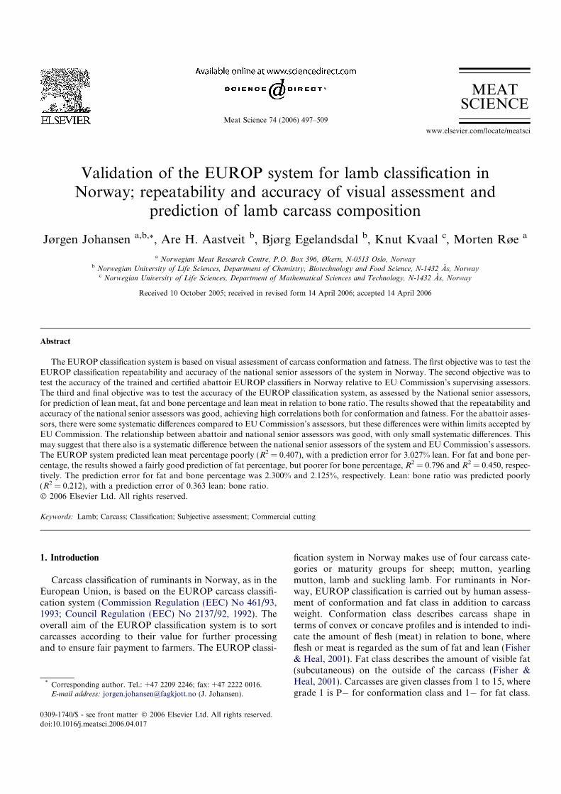
Validation of the EUROP system for lamb classification inNorway; repeatability and accuracy of visual assessment and

prediction of lamb carcass composition

Jørgen Johansen a,b,*, Are H. Aastveit b, Bjørg Egelandsdal b, Knut Kvaal c, Morten Røe a

a Norwegian Meat Research Centre, P.O. Box 396, Økern, N-0513 Oslo, Norwayb Norwegian University of Life Sciences, Department of Chemistry, Biotechnology and Food Science, N-1432 As, Norway

c Norwegian University of Life Sciences, Department of Mathematical Sciences and Technology, N-1432 As, Norway

Received 10 October 2005; received in revised form 14 April 2006; accepted 14 April 2006

Abstract

The EUROP classification system is based on visual assessment of carcass conformation and fatness. The first objective was to test theEUROP classification repeatability and accuracy of the national senior assessors of the system in Norway. The second objective was totest the accuracy of the trained and certified abattoir EUROP classifiers in Norway relative to EU Commission’s supervising assessors.The third and final objective was to test the accuracy of the EUROP classification system, as assessed by the National senior assessors,for prediction of lean meat, fat and bone percentage and lean meat in relation to bone ratio. The results showed that the repeatability andaccuracy of the national senior assessors was good, achieving high correlations both for conformation and fatness. For the abattoir asses-sors, there were some systematic differences compared to EU Commission’s assessors, but these differences were within limits accepted byEU Commission. The relationship between abattoir and national senior assessors was good, with only small systematic differences. Thismay suggest that there also is a systematic difference between the national senior assessors of the system and EU Commission’s assessors.The EUROP system predicted lean meat percentage poorly (R2 = 0.407), with a prediction error for 3.027% lean. For fat and bone per-centage, the results showed a fairly good prediction of fat percentage, but poorer for bone percentage, R2 = 0.796 and R2 = 0.450, respec-tively. The prediction error for fat and bone percentage was 2.300% and 2.125%, respectively. Lean: bone ratio was predicted poorly(R2 = 0.212), with a prediction error of 0.363 lean: bone ratio.Ó 2006 Elsevier Ltd. All rights reserved.

Keywords: Lamb; Carcass; Classification; Subjective assessment; Commercial cutting

1. Introduction

Carcass classification of ruminants in Norway, as in theEuropean Union, is based on the EUROP carcass classifi-cation system (Commission Regulation (EEC) No 461/93,1993; Council Regulation (EEC) No 2137/92, 1992). Theoverall aim of the EUROP classification system is to sortcarcasses according to their value for further processingand to ensure fair payment to farmers. The EUROP classi-

fication system in Norway makes use of four carcass cate-gories or maturity groups for sheep; mutton, yearlingmutton, lamb and suckling lamb. For ruminants in Nor-way, EUROP classification is carried out by human assess-ment of conformation and fat class in addition to carcassweight. Conformation class describes carcass shape interms of convex or concave profiles and is intended to indi-cate the amount of flesh (meat) in relation to bone, whereflesh or meat is regarded as the sum of fat and lean (Fisher& Heal, 2001). Fat class describes the amount of visible fat(subcutaneous) on the outside of the carcass (Fisher &Heal, 2001). Carcasses are given classes from 1 to 15, wheregrade 1 is Pÿ for conformation class and 1ÿ for fat class.

0309-1740/$ - see front matter Ó 2006 Elsevier Ltd. All rights reserved.

doi:10.1016/j.meatsci.2006.04.017

* Corresponding author. Tel.: +47 2209 2246; fax: +47 2222 0016.E-mail address: jorgen.johansen@fagkjott.no (J. Johansen).

www.elsevier.com/locate/meatsci

Meat Science 74 (2006) 497–509

MEATSCIENCE

Grade 15 is E+ conformation class and 5+ for fat class.High value for conformation class indicates a carcass withwell to excellent rounded muscles. High value on fat classindicates a carcass with a high degree of external fat (sub-cutaneous), and utilizes the relationship between externalfat and total fat content of carcass.

In Norway, human assessors carry out EUROP classifi-cation of lamb carcasses (manually) by sensory evaluationof carcasses. Classification of ruminant carcasses is tradi-tionally done by trained assessors because of the difficultyof identifying appropriate instrumental methods. The Nor-wegian Meat Research Centre (NMRC) (national seniorassessors) has been given the responsibility by the Norwe-gian classification board (Røe, 2002) to train and certifyabattoir assessors, using EU Commission photographicstandards. Abattoir assessors are supervised after they havefinished their training and certification, and are validatedseveral times annually by the national senior assessors.Certification is withdrawn from abattoir assessors if theyfail supervision and validation tests. The approval limitsfor certification and validation of assessors for the EUROPclassification system are described by the EU Commissionregulation (EC) No. 1215/2003. National senior assessorsare also supervised and validated annually by the EU Com-mission assessors. The foundation of the EUROP carcassclassification system is a 5-class system, legislated by theEU Commission (Regulation (EEC) No 2137/92, No461/93, 1992/1993; Commission Regulation (EEC) No461/93, 1993; Council Regulation (EEC) No 2137/92,1992). In Norway, EUROP carcass classification of lambcarcasses is carried out using 15 classes (5 classes with +and ÿ for each class), both for conformation and fat.The rules laid down by the EU Commission states thatabsolute maximum deviation (bias) between EU Commis-sion and abattoir assessors should not be larger than 0.3and 0.6 for conformation and fat class, respectively (Com-mission Regulation (EC) No 1215/2003, 2003). The slopeof a linear regression line (fitted) between EU Commissionand abattoir assessors should not deviate more than ±0.15and 0.30 from 1 for conformation and fat class, respectively(Commission Regulation (EC) No 1215/2003, 2003).

Pig carcasses are not classified, but graded instrumen-tally by measuring backfat and muscle depth as a predictorof lean meat percentage. At the same level of overall bodyfat, pigs have 68% of the dissectible fat subcutaneous, whilesheep and dairy cattle have 43% and 24%, respectively(Warriss, 2000). Beef cattle have a somewhat higher pro-portion of subcutaneous fat than dairy cattle. The greaterproportion of subcutaneous fat in pig carcasses makesgrading using instruments measuring backfat more accu-rate for pigs than for sheep and cattle. There is however,a lot of interest (Allen, 2003; Allen & Finnerty, 2001; Berg,Neary, Forrest, Thomas, & Kauffman, 1997; Cunha et al.,2003; Du & Sun, 2004; Fisher, 1990; Garrett, Edwards,Savell, & Tatum, 1992; Hopkins, Anderson, Morgan, &Hall, 1995; Kempster, Chadwick, Cue, & Granley-Smith,1986; Kirton, Mercer, & Duganzich, 1992; Stanford, Jones,

& Price, 1998; Swatland, Ananthanarayanan, & Golden-borg, 1994), both industrially and scientifically, to lookfor instrumental methods for ruminant species, i.e. opticalprobes and video image analysis (VIA). It can be arguedthat the use of the EUROP assessment scheme involvingtraining of assessors and the use of photographic standardsas reference points result in an evaluation system which isobjective in nature. However, since instrumental methodsusually are calibrated against known references for a givenset of parameters, visual assessment may be less stable dueto differences between operators plus the season-based nat-ure of lamb slaughtering. This is a major concern, evenwhen assessors are well trained, supervised and calibratedagainst photographic standards.

The main objectives of this study were to:

1. Study and identify the accuracy of the national seniorassessors using the EUROP classification system photo-graphic standards for lamb.

2. Study the abattoir EUROP classification accuracy inNorway compared with EU Commission’s assessorsusing the EUROP classification system photographicstandards for lamb.

3. Compare national senior vs. abattoir assessors withrespect to EUROP classification, and study the accuracyof the EUROP classification system for prediction oflean meat, fat and bone percentage and lean meat inrelation to bone ratio.

The first two objectives will identify the accuracy ofvisual assessment before the EUROP system is testedagainst carcass composition end-points.

2. Materials and methods

2.1. Trials

Three separate trials were carried out (Table 1).The assessors that participated in the different trials

were allocated into three levels: (1) Abattoir assessors, (2)national senior assessors (NMRC) and (3) EU Commissionassessors (Fig. 1). The abattoir assessors were trained andapproved assessors available and working at the selectedplants during the time of the study. National senior asses-sors were a group of three highly skilled assessors workingat the Norwegian Meat Research Centre. The EU Commis-sion assessors were a group of four highly skilled interna-tional assessors from Great Britain, France, Iceland andNorway. The photographic standards of the EU Commis-sion were used as the main reference point for lamb carcassclassification in all trials. The first trial was carried out inautumn of 2000 to check the repeatability of the nationalsenior assessors. The second trial was carried out inautumn of 2004 to validate the abattoir classification levelin Norway. The third trial was carried out in autumn of1999 to check the accuracy of the EUROP classificationsystem carried out by the national senior assessors for pre-

498 J. Johansen et al. / Meat Science 74 (2006) 497–509

diction of lean meat, fat and bone percentage and leanmeat: bone ratio. The reason that the verification and val-idation of the different levels of assessors was done after thecutting trial (trial 3), was related to the fact that the actualresults brought up the issue of improved documentation ofthe actual global validity of the results.

2.2. EUROP classification routines

In all the experiments, categories of animal, conforma-tion and fat class were assessed according to the EUROPguidelines made effective in Norway in 1996 (Røe, 2002).

The flow of supervision and validation is shown in Fig. 1.A 5-group system was introduced to compare the accuracyof 15 groups versus 5 groups. Both the 5-group and15-group systems are shown in Table 2 for comparison.

2.3. Raw data

2.3.1. Trial 1: EUROP classification repeatability

(accuracy) of national senior assessors

Forty lamb carcasses were sampled from a single Nor-wegian abattoir in the southeast part of Norway (GildeHed-Opp Rudshøgda). The carcasses were selected froma population classified by abattoir assessors (Table 3).

Three national senior assessors classified the 40 car-casses three times (triple test). The carcasses were arrangedin random order for each repetition.

2.3.2. Trial 2: Accuracy of abattoir EUROP classification in

Norway compared to EU Commission supervising assessors

Five hundred lamb carcasses (trial 2) were sampled fromfive different abattoirs distributed according to EUROPconformation and fat class during a 5-day trial in theautumn of 2004 (Table 4).

The carcasses were distributed as evenly and as practi-cally possible across a 15*15 grid (Table 5) of EUROPconformation and fat classes following the allocation ofabattoir assessors. Four EU Commission assessors classi-fied the 500 carcasses during the 5-day trial. Three out ofthe four assessors were regarded as more experienced,and their assessment was weighed with 2 compared to thelast, less experienced assessor, which was weighed with 1.All the assessments were averaged for further analysisaccording to the weighing of assessor into a ‘‘Gold Mean’’.

2.3.3. Trial 3: Accuracy of abattoir EUROP classification in

Norway compared to national senior assessors. Accuracy of

the EUROP classification system for prediction of lean meat,

fat and bone percentage and lean meat: bone ratio

Three hundred ninety five lamb carcasses from six differ-ent abattoirs distributed geographically across Norwaywere sampled for cutting at the NMRC pilot plant duringautumn of 1999. The largest abattoir (Gilde Hed-Opp Rud-shøgda) provided 298 lamb carcasses. The experimental

Fig. 1. Order of EUROP assessors. EU Commission assessors superior to

NMRC national (senior) assessors, and NMRC national (senior) assessors

superior to abattoir assessors.

Table 2

15-Point scale and 5-point scale used for EUROP conformation and fat class

Conformation class-15 E+ E Eÿ U+ U Uÿ R+ R Rÿ O+ O Oÿ P+ P PÿScale-15 15 14 13 12 11 10 9 8 7 6 5 4 3 2 1

Fat class-15 5+ 5 5ÿ 4+ 4 4ÿ 3+ 3 3ÿ 2+ 2 2ÿ 1+ 1 1ÿ

Conformation class-5 E U R O P

Scale-5 5 4 3 2 1

Fat class-5 5 4 3 2 1

Table 1

Description of trials

Trial Number of

animals (n)

Time of trial Objective

1 40 Autumn 2000 EUROP classification

repeatability (accuracy) of

national senior assessors

2 500 Autumn 2004 Accuracy of abattoir EUROP

classification in Norway

compared to EU Commission

supervising assessors

3 396 Autumn 1999 Accuracy of abattoir EUROP

classification in Norway

compared to national senior

assessors. Accuracy of the

EUROP classification system for

prediction of lean meat, fat and

bone percentage and lean meat to

bone ratio

J. Johansen et al. / Meat Science 74 (2006) 497–509 499

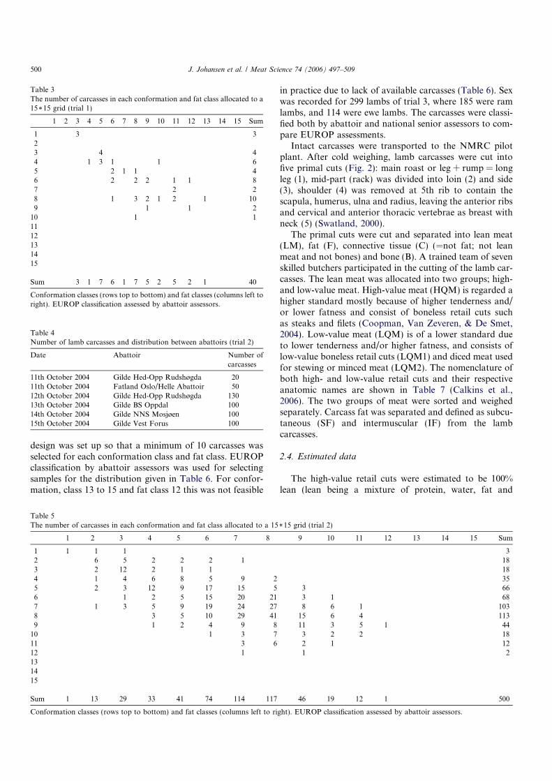
design was set up so that a minimum of 10 carcasses wasselected for each conformation class and fat class. EUROPclassification by abattoir assessors was used for selectingsamples for the distribution given in Table 6. For confor-mation, class 13 to 15 and fat class 12 this was not feasible

in practice due to lack of available carcasses (Table 6). Sexwas recorded for 299 lambs of trial 3, where 185 were ramlambs, and 114 were ewe lambs. The carcasses were classi-fied both by abattoir and national senior assessors to com-pare EUROP assessments.

Intact carcasses were transported to the NMRC pilotplant. After cold weighing, lamb carcasses were cut intofive primal cuts (Fig. 2): main roast or leg + rump = longleg (1), mid-part (rack) was divided into loin (2) and side(3), shoulder (4) was removed at 5th rib to contain thescapula, humerus, ulna and radius, leaving the anterior ribsand cervical and anterior thoracic vertebrae as breast withneck (5) (Swatland, 2000).

The primal cuts were cut and separated into lean meat(LM), fat (F), connective tissue (C) (=not fat; not leanmeat and not bones) and bone (B). A trained team of sevenskilled butchers participated in the cutting of the lamb car-casses. The lean meat was allocated into two groups; high-and low-value meat. High-value meat (HQM) is regarded ahigher standard mostly because of higher tenderness and/or lower fatness and consist of boneless retail cuts suchas steaks and filets (Coopman, Van Zeveren, & De Smet,2004). Low-value meat (LQM) is of a lower standard dueto lower tenderness and/or higher fatness, and consists oflow-value boneless retail cuts (LQM1) and diced meat usedfor stewing or minced meat (LQM2). The nomenclature ofboth high- and low-value retail cuts and their respectiveanatomic names are shown in Table 7 (Calkins et al.,2006). The two groups of meat were sorted and weighedseparately. Carcass fat was separated and defined as subcu-taneous (SF) and intermuscular (IF) from the lambcarcasses.

2.4. Estimated data

The high-value retail cuts were estimated to be 100%lean (lean being a mixture of protein, water, fat and

Table 3

The number of carcasses in each conformation and fat class allocated to a

15*15 grid (trial 1)

1 2 3 4 5 6 7 8 9 10 11 12 13 14 15 Sum

1 3 3

2

3 4 4

4 1 3 1 1 6

5 2 1 1 4

6 2 2 2 1 1 8

7 2 2

8 1 3 2 1 2 1 10

9 1 1 2

10 1 1

11

12

13

14

15

Sum 3 1 7 6 1 7 5 2 5 2 1 40

Conformation classes (rows top to bottom) and fat classes (columns left to

right). EUROP classification assessed by abattoir assessors.

Table 4

Number of lamb carcasses and distribution between abattoirs (trial 2)

Date Abattoir Number of

carcasses

11th October 2004 Gilde Hed-Opp Rudshøgda 20

11th October 2004 Fatland Oslo/Helle Abattoir 50

12th October 2004 Gilde Hed-Opp Rudshøgda 130

13th October 2004 Gilde BS Oppdal 100

14th October 2004 Gilde NNS Mosjøen 100

15th October 2004 Gilde Vest Forus 100

Table 5

The number of carcasses in each conformation and fat class allocated to a 15*15 grid (trial 2)

1 2 3 4 5 6 7 8 9 10 11 12 13 14 15 Sum

1 1 1 1 3

2 6 5 2 2 2 1 18

3 2 12 2 1 1 18

4 1 4 6 8 5 9 2 35

5 2 3 12 9 17 15 5 3 66

6 1 2 5 15 20 21 3 1 68

7 1 3 5 9 19 24 27 8 6 1 103

8 3 5 10 29 41 15 6 4 113

9 1 2 4 9 8 11 3 5 1 44

10 1 3 7 3 2 2 18

11 3 6 2 1 12

12 1 1 2

13

14

15

Sum 1 13 29 33 41 74 114 117 46 19 12 1 500

Conformation classes (rows top to bottom) and fat classes (columns left to right). EUROP classification assessed by abattoir assessors.

500 J. Johansen et al. / Meat Science 74 (2006) 497–509

ash). The lean percentage of the low-value retail cuts(lm1%) were estimated by chemical analysis (2006b),and the lean meat percentage of diced and minced meatproducts (lm2%) were estimated using AnylRay (ScanioA/S, 1997) at-line in the NMRC pilot plant. Total leanmeat content (LMC) was estimated using the weight ofall high-value retail cuts, and the lean percentage estima-tions of the low-value meat. Lean meat percentage(LM%) was estimated by dividing the total lean meat con-tent by the cold carcass weight, expressed as relative pro-portions (%):

LMC ¼ HQMþ lm1% � ðLQM1Þ þ lm2% � ðLQM2Þ;

LM% ¼ LMC=CCW � 100%:

Subcutaneous fat (SF) and manually separated intermuscu-lar fat (IF) was estimated to be 70% fat (30% mainly pro-teins and water). The fat percentage of LQM1 (f1%) wasestimated by the residue proportion from chemical analy-sis, and the fat percentage of LQM2 (f2%) by the residueproportion from AnylRay measurement. Total fat content(FC) was estimated using weight of SF + IF, and the fatestimations of LQM1 and LQM2. Fat percentage (F%)

Table 6

The number of carcasses in each conformation and fat class allocated to a 15*15 grid (trial 3)

1 2 3 4 5 6 7 8 9 10 11 12 13 14 15 Sum

1 19 5 19 24

2 5 16 7 3 5 31

3 9 12 8 29

4 2 23 14 4 1 44

5 6 14 9 3 6 5 43

6 1 1 12 11 10 9 6 3 2 1 56

7 1 4 5 2 8 3 1 2 1 27

8 3 5 5 6 3 1 23

9 1 2 4 4 1 3 15

10 4 3 8 9 9 4 2 2 41

11 1 1 5 3 9 9 3 1 32

12 1 2 1 3 2 1 10

13 3 1 1 2 1 3 8

14 2 2 2 2 2 1 2 11

15 1 1

Sum 29 37 56 72 49 44 59 29 9 7 4 29 395

Conformation classes (rows top to bottom) and fat classes (columns left to right). EUROP classification assessed by abattoir assessors.

Fig. 2. Lamb carcass primal cuts used in Norway.

Table 7

High-value and low-value meat; retail cuts

Name of retail cut Standard Major muscles

Lamb tenderloin High-value Psoas major, Psoas minor

Lamb loin High-value Longissimus, Complexus, Multifidus, Spinalis dorsi

Lamb inside round High-value Semimembranosus

Lamb leg roast (chump) High-value Semitendinosus, Biceps femoris, Rectus Femoris, Vastus lateralis, Vastus medialis,

Vastus intermedius

Lamb rib skin + flank for manufacturing Low-value Intercostal + abdominal muscles (flank)

Lamb shoulder clod roast Low-value Serratus ventralis, Subscapularis, Infraspinatus, Supraspinatus, Triceps brachii, Teres major

Lamb chuck Low-value Triceps brachii, Teres major, Longissimus

J. Johansen et al. / Meat Science 74 (2006) 497–509 501

was estimated by dividing the total fat content by the coldcarcass weight, expressed as relative proportions (%):

FC ¼ 0:7% � ðSFþ IFÞ þ f1% � ðLQM1Þ þ f2% � ðLQM2Þ;

F% ¼ FC=CCW � 100%:

All the soft tissues (LM, F, and C) were removed fromthe bones, and the total bone content (BC) was estimatedby weighing all the bones (B). Bone percentage (B%) wasestimated by dividing the total bone content by the coldcarcass weight, expressed as relative proportions (%):

BC ¼ B;

B% ¼ BC=CCW � 100%:

Lean meat to bone ratio (LM:B) was estimated by divid-ing the total lean content by the total bone content,expressed as a ratio between lean and bone:

LM : B ¼ LMC=BC:

2.5. Chemical analysis

Chemical analysis to estimate fat content in low-valueretail cuts was carried out by the Buchi-CaviezelÒ method(Norwegian Accreditation, 2006), NMKL23.

2.6. Statistical data analysis

Prediction of lamb carcass composition was carried outusing partial least square regression, PLS, modeling oneY-variable at the time (PLS1) (Martens & Martens, 2001),using the PLS_Toolbox for MATLAB (Wise et al., 2004).Cold carcass weight (CCW), EUROP conformation andfat class assessed by national senior assessors was chosenas predictors (X). Lean, fat and bone percent in additionto lean: bone ratio was chosen as dependent variables (Y).Validation of the prediction models was carried out usingfull leave-one-out cross validation, using root mean squareerror of cross validation (RMSECV) as diagnostic tool tofind a representative regression model. All the models werecentered to remove offset and reduce rank in the models.

3. Results

3.1. EUROP classification repeatability and accuracy of

national senior assessors

Table 8 shows the mean value and standard deviationsfor EUROP conformation and fat class for the national

senior assessors. There seemed to be some difference inassessment of conformation class between assessors. Asses-sor 3 tended to have a lower standard deviation than theother assessors. For fat class (Table 8), a larger differencebetween mean values was identified, both within andbetween assessors. However, there were no significant dif-ferences at 5% significance level.

From the correlation matrix (Table 9), assessor 3seemed to achieve a somewhat lower correlation coefficientfor conformation class than the other assessors did. For fatclass, the different national senior assessors were almostidentical with respect to variation in correlation betweenassessor and within tests (Table 10).

3.2. Accuracy of abattoir EUROP classification in Norway

compared to EU Commission supervising assessors

The agreement between the EU Commission assessorsshowed that 67.48% and 70.63% of the conformation andfat class assessments, respectively, were identical. The meanvalues and standard deviations in Table 11 show onlyminor differences and high conformity between EU Com-mission assessors.

Table 12 compared the mean values and standard devi-ations of abattoir and EU Commission assessors. The val-ues showed a difference in the classification level; theabattoir assessors seemed to over-classify (give a higherclass) the conformation class, and under-classify the fatclass (farmer-friendly classification). The standard devia-tions for conformation class between abattoir and EUCommission assessors are very similar. For fat class,

Table 8

Mean EUROP conformation and fat class (SD in parenthesis) of the three separate tests on 40 carcasses

Assessor n Conformation class Fat class

Test 1 Test 2 Test 3 Test 1 Test 2 Test 3

1 40 5.80 (2.64) 5.78 (2.56) 5.63 (2.55) 8.15 (3.08) 7.75 (2.94) 7.88 (3.01)

2 40 5.90 (2.71) 5.78 (2.61) 5.88 (2.71) 8.25 (3.07) 8.03 (3.20) 8.25 (3.26)

3 40 5.38 (2.54) 5.40 (2.57) 5.13 (2.41) 8.30 (3.14) 7.90 (3.19) 8.03 (3.09)

Three national senior assessors evaluated 40 lamb carcasses (n = 40; trial 1).

Table 9

Correlation coefficients (Pearson r) between three repeated tests (T1–T3)

of EUROP conformation class

Test n A1 A2 A3

T1 T2 T3 T1 T2 T3 T1 T2 T3

A1–T1 40 97.9 97.4 95.6 95.6 96.7 93.2 95.6 93.8

A1–T2 40 97.8 95.6 94.2 96.2 93.8 95.4 94.5

A1–T3 40 96.7 96.3 96.2 95.3 96.3 93.4

A2–T1 40 96.6 96.8 92.8 96.0 93.5

A2–T2 40 98.0 92.0 95.5 91.5

A2–T3 40 93.9 96.5 95.0

A3–T1 40 95.9 94.0

A3–T2 40 94.4

A3–T3 40

Three national senior assessors (A1–A3). 40 lamb carcasses (n = 40). Trial

1.

502 J. Johansen et al. / Meat Science 74 (2006) 497–509

standard deviations are smaller for abattoir than EU Com-mission assessors. Studying each abattoir with respect toconformation class assessment, one of them seemed toover-classify the carcasses significantly, one abattoir over-classified to some extent, two abattoirs where on target,while the last abattoir was under-classifying the carcasses.For fat class, only one abattoir was on target, three abatt-oirs were under-classifying and one abattoir was over-clas-sifying. Fig. 3 show the scatter plot between the averageabattoir and EU Commission assessments. The correla-tions (r) were 0.888 and 0.868 for conformation and fatclass, respectively. In this trial, the absolute deviationsbetween EU Commission and abattoir assessors were0.20 and 0.26 for conformation and fat class, respectively.

For the slope of the linear regression (fitted) line, the resultsshowed an offset of ÿ0.099 and ÿ0.184 from 1 for confor-mation and fat class, respectively.

3.3. Trial 3: Accuracy of abattoir EUROP classification in

Norway compared to national senior assessors. Accuracy of

the EUROP classification system for prediction of lean meat,

fat and bone percentage and lean meat: bone ratio

There were no significant differences between sexes forconformation class, carcass weight and lean meat percent-age. For fat class, fat and bone percentage there were clearsignificant differences between sexes. Ewe lambs were fatterthan ram lambs, and ram lambs had more bone than ewelambs. There seemed to be some difference in standarddeviations for conformation and fat class, where ram lambsshowed higher variability than ewe lambs for conformationclass, and ewe lambs showed higher variability than ramlambs for fat class. Correlation analysis was carried outwith or without sex as a factor. There was little or no dif-ference between the two alternatives, and it was decidednot to include sex in the following data analysis, in orderto achieve as many samples as possible from all abattoirs.

Fig. 4 shows the scatter plot between the national seniorand abattoir assessor with respect to EUROP classifica-tion. The correlations between national senior and abattoirassessors were 0.96 and 0.92 for conformation and fatclass, respectively. From the scatter plot, outliers, bothfor conformation and fat class were observed. These werecarcasses where abattoir assessors disagreed with thenational senior assessors, under-classifying both for con-formation and fat class. Otherwise, the abattoir andnational senior assessment seem to be synchronized bothfor conformation and fat class, with deviations spreadevenly across the scale. No significant bias or offset wasidentified.

Mean carcass weight (Table 13) for the samples washigher than for the whole population of 1999 (Røe,2000). Mean conformation class was also higher than thepopulation of 1999, but fat class was almost similar.

The correlation between carcass weight (CCW), confor-mation and fat class is shown in Table 14. The largest

Table 10

Correlation coefficients (Pearson r) between three repeated tests (T1–T3)

of EUROP fat class

Test n A1 A2 A3

T1 T2 T3 T1 T2 T3 T1 T2 T3

A1–T1 40 97.9 97.5 97.6 97.2 97.3 95.9 97.1 96.4

A1–T2 40 97.9 97.5 97.3 98.0 95.9 96.6 95.5

A1–T3 40 97.7 97.0 97.2 96.3 95.8 96.0

A2–T1 40 96.5 97.5 97.7 97.0 96.5

A2–T2 40 98.7 95.2 96.0 95.4

A2–T3 40 96.0 96.9 96.1

A3–T1 40 96.2 97.7

A3–T2 40 96.2

A3–T3 40

Three national senior assessors (A1–A3). 40 lamb carcasses (n = 40). Trial

1.

Table 11

Mean and standard deviation of EUROP conformation and fat class of

lamb carcasses

EU Commission

assessor

n Mean EUROP

conformation

class (SD)

Mean EUROP

fat class (SD)

1 500 6.68 (2.16) 6.73 (2.01)

2 500 6.66 (2.06) 6.75 (2.01)

3 500 6.68 (2.21) 6.64 (2.08)

4 500 6.69 (2.09) 6.69 (1.99)

EU Commission assessors. Trial 2.

Table 12

Mean and standard deviation of EUROP conformation and fat class of lamb carcasses

Date n EUROP conformation class EUROP fat class

Abattoir Gold mean Abattoir Gold mean

11th October 2004a 100 5.88 (1.45) 5.99 (1.66) 6.27 (1.46) 6.57 (1.56)

12th October 2004 100 7.34 (1.63) 7.32 (1.54) 7.44 (1.73) 7.49 (1.59)

13th October 2004 100 7.47 (1.72) 7.14 (2.00) 5.60 (1.72) 6.86 (1.68)

14th October 2004 100 8.44 (2.09) 7.42 (2.34) 7.46 (2.41) 7.05 (2.29)

15th October 2004 100 5.58 (2.14) 5.55 (2.13) 4.75 (1.84) 5.61 (2.22)

Total 500 6.88 (2.07) 6.68 (2.10) 6.31 (2.12) 6.57 (2.43)

Abattoir assessors vs. EU Commission assessors. Trial 2.a For 11th of October 30 carcasses from the Rudshøgda abattoir the 12th of October was included in addition to the 70 original carcasses form the 11th

of October.

J. Johansen et al. / Meat Science 74 (2006) 497–509 503

correlations were found between bone and lean: bone ratio(r = ÿ0.87), fat class and fat percentage (r = 0.86) and con-formation class and CCW (r = 0.84).

The heaviest carcasses both have high conformation andfat class. One exemption was a group of lean, highly con-formed (class 12 to 15) carcasses, yielding a somewhat neg-ative correlation between CCW and conformation classesfor high conformation carcasses (Table 15).

The results from prediction of lean meat percentage(Fig. 5) showed that 40.7% of the variation was explainedusing CCW and EUROP conformation and fat class aspredictors. The prediction error (RMSECV) was 3.027%lean. For 5 EUROP classes for conformation and fat

instead of 15 classes, RMSECV was 3.253. The followingprediction equation was extracted for lean percentage (15classes) from the regression analysis:

LM% ¼ 63:71ÿ 0:111 � CCW

þ 0:533 � EUROP Conformation Class

ÿ 1:158 � EUROP Fat Class:

EUROP fat class seemed to be the largest predictor,whereas high fat class yielded a lower lean percentage.

For fat percentage, Fig. 6 showed that 73.7% of thevariation was explained using the selected predictors. Theprediction error was 2.395% fat. Using 5 groups instead

Fig. 3. Scatter plot. Average assessment EU Commission assessors (y-axis) vs. average abattoir assessors (x-axis) (n = 500). Conformation and fat class.

Fig. 4. Scatter plot. Average assessment NMRC assessors (y-axis) vs. average abattoir assessors (x-axis) (n = 395). Conformation and fat class.

Table 13

Descriptive statistics, trial 3, n = 395

Parameter n Mean SD Min. Max.

CCW 395 19.20 5.55 7.22 33.50

Conformation class 395 6.51 3.50 1 15

Fat class 395 5.77 2.57 1 12

Lean percent 395 63.71 3.93 45.10 73.50

Fat percent 395 13.88 4.67 6.59 33.21

Bone percent 395 22.41 2.87 15.70 35.38

Lean: bone ratio 395 2.89 0.41 1.64 4.31

1. National senior assessors, EUROP classification.

2. Cold carcass weight, kg.

3. Percentage tissue of CCW (%).

Table 14

Correlation coefficients (Pearson) EUROP classification and cutting

variables

Confa Fata CCWb Leanc Fatc Bonec

Fata 0.63

CCWb 0.84 0.74

Leanc ÿ0.15 ÿ0.59 ÿ0.31

Fatc 0.51 0.86 0.65 ÿ0.79

Bonec ÿ0.63 ÿ0.60 ÿ0.63 ÿ0.08 ÿ0.54

Lean: bone 0.47 0.22 0.38 0.53 0.09 ÿ0.87

a National senior assessors, EUROP classification.b Cold carcass weight, kg.c Percentage tissue of CCW (%).

504 J. Johansen et al. / Meat Science 74 (2006) 497–509

of 15, the prediction error was larger (2.735). The followingprediction equation was extracted for fat percentage fromthe regression analysis:

F% ¼ 13:88þ 0:217 � CCW

ÿ 0:318 � EUROP Conformation Class

þ 1:472 � EUROP Fat Class:

EUROP fat class was the largest predictor, where highfat class yielded high fat percentage. Due to a non-lineartrend between predicted and measured values (Fig. 6), dif-ferent fat transformations of fat percent data were tested.The natural logarithmic transformations seemed toimprove predictions better than other types of transforma-tions (square root, logarithmic, polynomic).

By transforming data, the explained variance increasedfrom 73.7% to 79.6% of the variation in fat percentage

(Fig. 7) and the predicted vs. measured fit became more lin-ear. Transformation of data yielded a prediction error of2.30, which was smaller than the non-transformed data.The following prediction equation was extracted for ln(natural logarithm) fat percentage from the regressionanalysis:

ln F% ¼ 2:58þ 0:0163 � CCW

ÿ 0:0192 � EUROP Conformation Class

þ 0:0993 � EUROP Fat Class:

For bone percentage, Fig. 8 showed that 45.0% of thevariation was explained using the selected predictors. Pre-diction error was 2.125% bone. Fat class seemed to bethe largest predictor, whereas high fat class yielded lowbone percentage. High level of all the predictors yieldedlow level of bone percentage. Some non-linearity seemed

Table 15

Mean carcass weight (kg) per conformation and fat class (trial 3)

C F

1 2 3 4 5 6 7 8 9 10 11 12 Avg.

1 9.83 9.87 12.39 10.07

2 11.81 13.32 12.67 14.16 12.44

3 12.30 14.25 13.23 14.05 13.63

4 14.81 14.76 15.83 16.62 14.70 15.83

5 18.00 17.92 17.64 18.14 19.30 17.92 18.03

6 19.82 15.36 19.30 19.67 18.46 18.58 25.62 18.92 19.20

7 18.10 17.08 21.09 19.45 21.35 21.62 24.21 24.59 20.78

8 20.73 21.10 22.96 21.86 23.64 24.65 21.72 28.05 22.53

9 21.92 20.14 22.99 22.39 23.95 23.74 24.92 22.00 22.94

10 21.82 24.38 23.88 24.69 23.90 24.41 27.23 28.39 25.55 24.93

11 28.48 22.58 24.02 23.72 26.29 26.11 28.82 29.41 29.29 25.65

12 19.02 23.98 24.05 23.36 26.73 27.62 25.40 24.63

13 25.10 17.44 25.36 25.09 23.62

14 27.98 23.29 33.50 27.21

15 20.59 21.60 20.93

Avg. 9.83 12.63 15.62 15.44 18.15 20.17 21.63 23.18 24.62 24.78 25.28 28.67 19.20

Conformation class (C) (rows) and fat class (F) (columns).

45 50 55 60 65 70 7556

58

60

62

64

66

68

70

72

74

Y Measured 1

Y C

V P

redic

ted 1

Lean percentage

CCW CONF CLASS FAT CLASS-1.2

-1

-0.8

-0.6

-0.4

-0.2

0

0.2

0.4

0.6

Variable

Re

gr.

Co

eff.

Lean percentage

Fig. 5. Regression plot predicted vs. measured (left). Regression coefficients (right) for carcass weight (CCW), EUROP conformation and fat class. Lean

percentage.

J. Johansen et al. / Meat Science 74 (2006) 497–509 505

to be present between predicted and measured values, butdifferent transformations did not improve predictions.The following prediction equation was extracted for bonepercentage from the regression analysis:

B% ¼ 22:41ÿ 0:075 � CCW

ÿ 0:257 � EUROP Conformation Class

ÿ 0:333 � EUROP Fat Class:

For lean: bone ratio, Fig. 9 showed that 21.2% of thevariation was explained using the selected predictors. Pre-diction error was 0.363 lean: bone ratio. Conformationclass seemed to be the largest predictor, whereas high con-formation class yielded a higher lean: bone ratio. Differenttransformations of data did not improve predictions. Thefollowing prediction equation was extracted for lean: boneratio from the regression analysis:

L : B ¼ 2:89þ 0:161 � CCW

þ 0:445 � EUROP Conformation Class

ÿ 0:185 � EUROP Fat Class:

4. Discussion

The overall aim of the EUROP classification system isto sort carcasses according to their value presently definedby the variables CCW, fat, lean and lean: bone ratio, andthereby ensure fair payment to farmers. In addition, highrepeatability and reproducibility between classifiers ensurefair payment to farmers. The classifiers are expected to dothe same job, independent of geographical location andtime. The EU Commission assessors concluded that devia-tions were present between and within Norwegian abatt-oirs, but the deviations were within EU Commissionlimits for validation and approval of EUROP classificationcertification, especially for fat class in spite of the observedsystematic bias. The EU Commission limits for fat classifi-cation are less restricted than for conformation class. Thisis due to prognosis indicating that fat class is more difficultto assess than conformation class. Nevertheless, the valida-tion of abattoir classification against EU level in Norwayshowed that the average Norwegian abattoir assessor weresomewhat farmer-friendly, over-classifying conformation

5 10 15 20 25 30 355

10

15

20

25

Y Measured 1

Y C

V P

redic

ted 1

Fat percentage

CCW CONF CLASS FAT CLASS-0.4

-0.2

0

0.2

0.4

0.6

0.8

1

1.2

1.4

1.6

Variable

Re

gr.

Co

eff.

Fat percentage

Fig. 6. Regression plot predicted vs. measured (left). Regression coefficients (right) for carcass weight (CCW), EUROP conformation and fat class. Fat

percentage.

1.8 2 2.2 2.4 2.6 2.8 3 3.2 3.42

2.5

3

3.5

Y Measured 1

Y C

V P

red

icte

d 1

Ln Fat percentage

CCW CONF CLASS FAT CLASS-0.02

0

0.02

0.04

0.06

0.08

0.1

Variable

Re

gr.

Co

eff.

ln Fat percentage

Fig. 7. Regression plot predicted vs. measured (left). Regression coefficients (right) for carcass weight (CCW), EUROP conformation and fat class.

Natural logarithmic transformation (ln) of fat percentage.

506 J. Johansen et al. / Meat Science 74 (2006) 497–509

class and under-classifying fat class. For fat class, the aver-age abattoir assessor seemed to squeeze their classificationassessment towards the mean value (lower standard devia-tion than EU Commission assessors). This could be due tothe fear of assessing extreme values caused by lack of train-ing, infrequent number of extreme carcasses during workhours or biased training by the national senior assessors.There was also some variation between abattoirs, wheresome abattoirs performed poorer than others. This demon-strated the different level and lack of accuracy betweenabattoirs with respect to carcass classification despite thefact that Norway has a good certification system in accor-dance with the EU Commission. There was a good correla-tion within national senior assessors, and the correlationwith respect to abattoir assessment was also good. The sys-tematic bias and offset between abattoir and EU Commis-sion may also be valid for the relationship between EUCommission and national senior assessors, since nationalsenior assessors are responsible for training and supervis-

ing abattoir assessors. This may be interpreted that abat-toir assessors have adapted the bias and offset from theirtraining and supervision from the national senior assessors.

The main predictor of lean meat percent seems to be fatclass; high fat class yields low lean percentage. This is dueto the negative correlation between fat and lean meat per-centage. EUROP predicted fat percent well, with fat classas the main predictor. Transformation with natural loga-rithm seemed to improve predictions, mainly due to theassessors’ uncertainty for high fat classes. Bone percentagewas poorly predicted by EUROP, but the main trend wasthe negative correlation between bone percentage andEUROP + CCW variables; increasing weight, higher con-formation and fatness yields a lower bone percentage.Fat class was the most important predictor, which maybe due to the large difference in growth rate of fat andbone, as a function of carcass weight. Lean: bone ratio isa derivative of muscle: bone ratio, which describes the rela-tionship between lean and bone percentage. Lean: bone,

15 20 25 30 35 4018

19

20

21

22

23

24

25

26

27

Y Measured 1

Y C

V P

red

icte

d 1

Bone percentage

CCW Conf class Fat class-0.35

-0.3

-0.25

-0.2

-0.15

-0.1

-0.05

0

Variable

Re

gr.

coe

ff.

Bone percentage

Fig. 8. Regression plot predicted vs. measured (left). Regression coefficients (right) for carcass weight (CCW), EUROP conformation and fat class. Bone

percentage.

1.5 2 2.5 3 3.5 4 4.52.5

2.6

2.7

2.8

2.9

3

3.1

3.2

3.3

3.4

3.5

Y Measured 1

Y C

V P

red

icte

d 1

Lean:bone

CCW Conf class Fat class-0.03

-0.02

-0.01

0

0.01

0.02

0.03

0.04

0.05

0.06

Variable

Re

gr.

co

eff.

Lean:bone

Fig. 9. Regression plot predicted vs. measured (left). Regression coefficients (right) for carcass weight (CCW), EUROP conformation and fat class. Lean:

bone ratio.

J. Johansen et al. / Meat Science 74 (2006) 497–509 507

however, describes the leanness, not muscle, of the carcassrelated to bone. The major problem with muscle: boneratio is that it does not take into consideration the fat con-tent of the carcass. All carcasses contain fat in varying pro-portions primarily dependent upon degree of maturity ofthe animal from which the carcass came. And, in mostcases, carcasses with high muscle: bone ratios also havehigh fat: bone ratios so that they may have lower percent-age of carcass muscle than carcasses with low muscle: boneratios (Thonney, 2006). A high level of lean: bone ratio issomewhat correlated with conformation, and may serveas a measurement of muscularity of the carcass adjustingfor the level fatness. A high lean: bone ratio generally yieldsa high-muscled lean carcass. Compared to previous studies(Warriss, 2000), the lamb carcasses in this trial were rela-tively lean (13.88% fat). The estimated lean percentagewas similar to Warriss (2000) but bone percentage was sig-nificantly larger. The difference in fat and bone percentagesbetween this trial and other studies may be because Norwe-gian lamb carcasses are lower in carcass weight than thoseof Warriss (2000) yielding carcasses with higher percentageof bone and lower percentage of fat. There may also besome influence from cutting error, where the butchers lefttoo much tissue on the bones, but it is not expected thatthis error should be any larger than in any other study sim-ilar to this trial.

5. Conclusion

For abattoir assessors, there were some systematic dif-ferences compared to EU Commission’s assessors carryingout EUROP classification, but these differences were withinEU Commission limits. In average, the abattoirs seemed toover-classify conformation class and under-classify fatclass (farmer-friendly classification). The relationshipbetween abattoir and the national senior assessors wasgood with no systematic bias or offset. This suggests thatthe same bias and offset is to be found between nationalsenior and EU Commission assessors as for abattoir vs.EU Commission’s assessors. For prediction of the carcasscomponent parameters, lean meat and bone percentagewas not very accurate by the EUROP system. Predictionof fat percentage was fairly accurate, and yielded the mostaccurate prediction of the carcass component parameters.Lean: bone ratio was predicted poorly, and yielded thepoorest predictions of all parameters.

References

Allen, P. (2003). Beef carcass grading in Europe and USA – The prospects

for using VIA systems. In 49th ICoMST (pp. 96–101).

Allen, P., & Finnerty, N. (2001). Mechanical grading of beef carcasses.

TEAGASC, Report.

Berg, E. P., Neary, M. K., Forrest, J. C., Thomas, D. L., & Kauffman, R.

G. (1997). Evaluation of electronic technology to assess lamb carcass

composition. Journal of Animal Science, 75, 2433–2444.

Calkins, C., Jones, S., Carpenter, B., Minary, R., Brewster, R., Withing,

K., et al. (2006). Bovine myology and muscle profiling. University of

Nebraska, Lincoln; University of Florida; National Cattlemen’s Beef

Association; Cattlemen’s Beef Board. Available from http://

bovine.unl.edu.

Cunha, B. C. N., Belk, K. E., Scanga, J. A., LeValley, S. B., Tatum, J. D.

& Smith, G. C. (2003). Development and validation of equations

utilizing lamb vision system (LVS) output to predict lamb carcass

fabrication yields. In 49th ICoMST (pp. 341–342).

Commission Regulation (EEC) No 461/93. Commission Regulation

(EEC) No 461/93 of 26 February laying down detailed rules for the

Community scale for the classification of carcasses of ovine animals.

Commission regulation (EEC) No. 461/93.

Community scale for the classification of carcasses of ovine animals of

1992/1993. Regulation (EEC) No 2137/92, No 461/93.

Commission Regulation (EC) No 1215/2003 of 7 July 2003 amending

Regulation (EEC) No 344/91 laying down detailed rules for applying

Council Regulation (EEC) No 1186/90 to extend the scope of the

Community scale for the classification of carcasses of adult bovine

animals. No. 1215/2003.

Coopman, F., Van Zeveren, A., & De Smet, S. (2004). Comparison of

slaughter characteristics of ‘‘S’’ and ‘‘E’’ class slaughter bulls of the

double-muscled Belgian Blue beef breed using a commercial cutting

method. Vlaams Diergeneeskundig Tijdschrift, 73, 170–175.

Council Regulation (EEC) No 2137/92 of 23 July 1992 concerning the

Community scale for the classification of carcasses of ovine animals

and determining the Community standard quality of fresh or chilled

sheep carcasses and extending Regulation (EEC) No 338/91. Council

regulation (EEC) No 2137/92.

Du, C.-J., & Sun, D.-W. (2004). Recent developments in the application of

image processing techniques for food quality evaluations. Trends in

Food Science & Technology, 15, 230–249.

Fisher, A. V. (1990). New approaches to measuring fat in the carcasses of

meat animals. In J. D. Wood & A. V. Fisher (Eds.), Reducing fat in

meat animals (pp. 255–343). Amsterdam: Elsevier Applied Science.

Fisher, A., & Heal, J. (2001). Carcass classification. Beef & Sheep 2001, p.

314. Livestock Knowledge Transfer, a DEFRA initiative, operated by

ADAS/IGER/University of Bristol.

Garrett, R. P., Edwards, J. W., Savell, J. W., & Tatum, J. D. (1992).

Evaluation of the Hennessy grading probe to predict yields of lamb

carcasses fabricated to multiple end points. Journal of Animal Science,

70, 1146–1152.

Hopkins, D. L., Anderson, M. A., Morgan, J. E., & Hall, D. G. (1995). A

probe to measure GR in lamb carcasses at chain speed. Meat Science,

39, 159–165.

Kempster, A. J., Chadwick, J. P., Cue, R. I., & Granley-Smith, M. (1986).

The estimation of sheep carcass composition from fat and muscle

thickness measurements taken by probes. Meat Science, 16, 113–

126.

Kirton, A. H., Mercer, G. J. K., & Duganzich, D. M. (1992). Grading

probes for lamb carcasses. In Twenty-seventh meat industry research

conference.

Martens, H., & Martens, M. (2001). Multivariate analysis of quality – An

introduction. New York: Wiley.

Røe, M. (2000). Annual report: classification and weight results for 1999.

Norwegian Meat Research Centre, Norway.

Røe, M. (2002). Klassifiseringshandboken. Norwegian Meat Research

Centre (in Norwegian).

Scanio A/S. (1997). Scanio scanalyzer Ver. 7.00 – Manual.

Stanford, K., Jones, S. D. M., & Price, M. A. (1998). Methods of

predicting lamb carcass composition: a review. Small Ruminant

Research, 29, 241–254.

Swatland, H. J., Ananthanarayanan, S. P., & Goldenborg, A. A. (1994). A

review of probes and robots: implementing new technologies in meat

evaluation. Journal of Animal Science, 72, 1475–1486.

Swatland, H. J. (2000). Norway – lamb cuts. Meat cuts and muscle foods.

Nottingham University Press (pp. 137–138).

The Norwegian Institute for Food and Environmental Analysis –

Norwegian Accreditation. NS-EN ISO/IEC 17025 – TEST001

(2006). P12 – Chemical Analysis, Norwegian Accreditation.

508 J. Johansen et al. / Meat Science 74 (2006) 497–509

Thonney, M. (2006). Animal Science 360. Beef Cattle 2006. Electronic

lecture. Animal Sciences at Cornell University. Web page.

Warriss, P. D. (2000). Meat science – An introductory text. 0-85199-424-5.

CABI Publishing.

Wise, B. M., Gallagher, N. B., Bro, R., Shaver, J. M., Windig, W. &

Koch, R. S. (2004). PLS_Toolbox 3.5 for use with MATLABä.

Eigenvector Research, Inc., 830 Wapato Lake Road, Manson, WA

98831, USA.

J. Johansen et al. / Meat Science 74 (2006) 497–509 509

Paper II

1

The reference butcher panel’s precision and reliability of dissection for

calibration of lamb carcass classification in Norway

J. Kongsroa,b*, B. Egelandsdalb, K. Kvaalc, M. Røea, A.H. Aastveitb

a Animalia – Norwegian Meat Research Centre, P.O. Box 396 Økern, N-0513 Oslo, Norway

b Dept. of Chemistry, Biotechnology and Food Science, Norwegian University of Life Sciences, P.O. Box 5003, N-1432 Ås, Norway

c Dept of Mathematical Sciences and Technology, Norwegian University of Life Sciences, P.O. Box 5003, N-1432 Ås, Norway

Abstract

Dissection of lamb carcasses is used as a reference method for maintenance and development

of lamb carcass classification and grading. The accuracy in terms of precision and reliability

of lamb carcass dissection as a reference method has never been quantified. The reference

method in Norway is performed by a skilled butcher panel at Animalia – Norwegian Meat

Research Centre. Lamb carcass dissection was studied with respect to precision and reliability

of repeated measurements using splitting of lamb carcasses (left-right). The carcass dissection

traits yield and carcass composition were estimated for both sides, and the precision and

reliability was quantified for the butcher panel. The overall precision and reliability was

acceptable for carcass composition traits, however the results for sub-primal yield and

composition was somewhat poorer. The precision (CV %) of the carcass tissues fat, muscle

and bone were 4.34, 2.27 and 3.19 for tissue weights, and 4.11, 1.19 and 3.00 for tissue

proportions, respectively. The reliabilities of the carcass tissues were 0.98, 0.96 and 0.85 for

tissue weights, and 0.93, 0.80 and 0.90 for tissue proportions, respectively. The muscle tissue

was most precise, while the fat tissue was most reliable. With respect to sub-primal

dissection, the lamb breast seem to be difficult for the butchers to dissect, and needs special

attention when setting up a dissection of lamb carcasses.

Keywords: Dissection, lamb carcass classification, precision, reliability

* Corresponding author. Phone: +4722092246; Fax: +4722220016.

E-mail address: jorgen.kongsro@animalia.no (Jørgen Kongsro)

2

Introduction

The main purpose of dissection of lamb carcasses in Norway is to evaluate carcass

composition and slaughter maturity, and to act as a reference method for classification and

grading methods for lamb (i.e. visual appraisal, visible light probing, Video Image Analysis

(VIA) and ultrasound) (Røe, 1998). Although international reference methods had been

developed for pork and beef carcasses in the late seventies and early eighties, no such method

had been agreed for sheep carcasses until (Fisher and de Boer, 1994) presented their EAAP

standard method of sheep carcass assessment in the nineties. However, like the other

reference methods for pork and beef, the EAAP standard method was not quantified with

respect to precision and reliability. The EUROP classification system for lamb carcasses is a

classification scale laid down by Council Regulation (EEC) No 2137/92, where the

classification must be made on the basis of conformation and the degree of fat cover and the

combination of these two criteria enables carcasses of ovine animals to be divided into classes

(Council Regulation (EEC) No 2137/92, 1992). The regulation provided for a Community-

wide carcass classification standard with the object of improving market transparency in the

sheepmeat sector. The details for the classification system were laid down in Commission

Regulation (EEC) No 461/93, where the market price for ovine carcasses are to be established

on the basis of the EUROP scale, and conformation and fat classes are described in the Annex

(Commission Regulation (EEC) No 461/93, 1993). After the implementation of EUROP in

Norway in 1996, dissection is still used as an objective measure for carcass quality in addition

to EUROP conformation and fat class, and is regularly used as a calibration method to check

for relationship between EUROP classes and carcass composition (muscularity, lean meat

yield and fat content). In addition, dissection is important for breeding traits, which rely solely

on the dissection as an objective measure for selection. The lamb carcasses are dissected by a

reference butcher panel at the pilot plant at Animalia – Norwegian Meat Research Centre

(Johansen et al., 2006). The butcher panel’s dissection of lamb carcasses in Norway involves

the dissection of 5 primal cuts (leg, loin, side, breast and shoulder) from a lamb carcass.

For pig carcass classification, the estimated accuracy of the EU reference dissection

method was presented quite recently (Nissen et al., 2006). The authors found variations

between butchers from different EU countries with respect to lean meat percentage and

jointing of carcasses. The maximum difference of Lean Meat Percentage (LMP) between two

butchers was found to be 1.9 %. The authors also found that even if the EU reference

dissection method for pig carcasses was well described by (Walstra and Merkus, 1996), some

deviations was observed during their experiment, especially the lack of description of

3

anatomical lines in the forepart or shoulder. For dissection of lamb carcasses, the jointing is

somewhat different from pork dissection. The forepart of lamb is jointed into two primal cuts;

shoulder and breast. The distribution of fat in lamb carcasses is also somewhat different

compared to pig carcasses. Some deviations and lack of description was also found in the

EAAP standard method for sheep carcass assessment described by Fisher and de Boer (1994),

especially for neck and thorax (breast) jointing and dissection. A more detailed description

and methodical framework is needed for the dissection of lamb carcasses.

As a reference for carcass classification and grading, it is important that the precision and

reliability of dissection are as high as possible. Dissection or determination of carcass

composition is the basis for development and maintenance of carcass grading and

classification, and the accuracy of the reference dissection method for lamb and sheep needs

to be described and quantified.

The objective of this study was to describe and quantify the precision and reliability of

lamb carcass dissection as a reference method for lamb carcass classification in Norway

performed the Animalia reference butcher panel. In addition, a methodical framework was put

forward for future studies and regular inspection of the accuracy of lamb carcass dissection in

Norway.

4

Materials & methods

Slaughter and experimental design

Sixty (60) half carcasses (30 whole carcasses) were selected from cold storage (-18oC)

according to EUROP fat class to ensure as much variation in fatness as possible. The lambs

were slaughtered during October 2006 at one large abattoir in central Norway (Rudshøgda),

and were frozen and stored after conditioning for a maximum of 5 days post-slaughter (4oC).

The carcasses were thawed one week prior to cutting, in batches of 10 carcasses per week, in

a refrigerated room (0-4oC) during January 2007. The weight-loss from thawing was closely

monitored, and the mean weight loss from warm carcass weight to thawed carcass was 3.95

%. The carcass weight used to obtain and estimate dissection traits in this study, is the cold

carcass weight before dissection, after thawing. The 30 carcasses were distributed evenly

among five skilled reference butchers at the Animalia (Norwegian Meat Research Centre)

pilot plant during January 2007, according to an experimental design using EUROP fat class

(Tab. 1).

Table 1. Experimental design; butcher panel dissection of lambs. Cold carcass weight (CCW), EUROP conformation and fat class given butchers A-E. Number (n) of whole (1/1) carcasses and mean values (standard deviations in parenthesis). Butcher -> A B C D E Total n 6 6 6 6 6 30 CCW (kg) 17.10

(2.62) 16.88 (1.94)

17.13 (2.27)

15.92 (2.77)

16.40 (1.05)

16.69 (2.21)

Conformation class

5.50 (1.31)

5.83 (1.75)

6.17 (1.40)

5.33 (0.98)

5.17 (0.72)

4.80 (1.92)

Fat class 5.50 (2.15)

4.67 (1.97)

5.33 (2.15)

4.50 (1.88)

4.00 (1.04)

5.60 (1.30)

The reference butcher panel

The pilot plant at Animalia acts as a reference dissection panel for carcass classification and

grading in Norway. The reference butcher panel consists of 5 butchers, who are employed at

the Animalia pilot plant. The butchers are skilled professionals who perform dissection

regularly for industry and scientific use. The total numbers of carcasses dissected annually are

approximately 2800 pig, 70 beef and 200 lamb carcasses.

Dissection and cutting traits

The Norwegian dissection of lambs is based on guidelines supervised by Gunnar Malmfors,

SLU, Sweden, exemplified in a Swedish Master Thesis (Einarsdottir, 1998), and the

guidelines presented in the EAAP standard method by Fisher and de Boer (1994). The

5

carcasses were split into 2 halves along the spinal column and the halves were jointed into 3

primal cuts; forepart, midpart and backpart (legs). The mid-part (lumbar region) of the carcass

was divided into sub-primals loin (rack) and side (flank) (Fig. 1). The sub-primal shoulder

(proximal thoracic limb) was removed at the 5th rib to contain the large anterior (forepart)

bones (scapula, humerus, ulna and radius), leaving the anterior ribs and cervical and anterior

thoracic vertebrae as sub-primal breast with neck (Swatland, 2000) (Fig. 1). The backpart

(proximal pelvis limb) was cut into lamb legs, long style with sirloin. For all primals and sub-

primals, the first operation in the dissection process was the removal of subcutaneous fat.

Muscles were then removed from bones, either singly or in groups. Finally, intermuscular fat

was trimmed from large muscles (steaks and filets), and bones and items such as tendons,

lymph nodes etc. are separated from the major tissues (Fisher and de Boer, 1994). The smaller

muscles or trimmings containing some fat were classified as manufacturing meat. Jointing

and dissection of both halves from each carcass was performed by the same butcher (A – E),

and 6 (12 halves) carcasses were dissected by each butcher (Tab. 1). In average, one butcher

dissected two carcasses (four halves) per day. Detailed figures of dissection of sub-primals are

shown in Figure 2.

6

1

2

3

4

5

Figure 1. Norwegian lamb cuts. Sub-primals shoulder (proximal thoracic limb) (1), breast (neck and thorax) (2), side (lumbar, ventral side) (3), loin (lumbar, dorsal side) (4) and leg (proximal pelvic limb) (5). Surrounding pictures: Different retail products derived from lamb carcass sub-primal cuts.

7

Breast

Loin

Leg

Shoulder

Side Figure 2. Dissection of a lamb carcass; sub-primal cuts. The five sub-primal cuts from left to right: breast, loin (top), shoulder and leg (middle) and side (bottom). The sub-primals are dissected into steaks and filets (large muscles), manufacturing meat, fat, bone and waste (tendons, lymph nodes etc.).

The fat content of manufacturing meats was estimated using AnylRay (Scanio A/S, 1997)

at-line in the NMRC pilot plant. Estimates of soft tissues were obtained by calculating the fat-

trimmed (lean) muscles from filets and steaks, fat content in manufacturing meats and the

separable fat (subcutaneous and intermuscular fat) from dissection. The carcass composition

8

data was reported as weights (kg or g) or as proportions (%), either as sums of the ½ carcass,

or as sub-primal yield or composition.

Statistical analysis

All data analysis were performed using MATLAB Version 7.4.0.287 (R2007a), January 29,

2007, Copyright 1984-2007, The MathWorks, Inc (The MathWorks, 2007). The difference in

dissection traits were calculated using absolute difference between the two sides (left-right).

The precision of cutting was measured by using the relative standard deviation (RSD) of the

difference between the two carcass halves (Breidenstein et al., 1964), using the ratio of the

standard deviation of the difference between the two sides (left-right) and the average carcass

side (left-right), sub-primal or tissue weight / proportion. The RSD was expressed as a fraction,

but more usually as a percentage and was then called coefficient of variation (CV) (van

Reeuwijk and Houba, 1998) (1):

%100..

xMean

differenceofdsCV = (1)

The reliability (REL) of dissection was defined as the correlation (r) between the repeated

measurements (the two carcass sides) (2):

222

22),cov(

σσσ

σσ

σσ ++

+==

CB

CB

rl

rl XXREL (2)

where l is left, and r right side.

The effect carcass side (left-right) on carcass and dissection traits, and carcass weight on

differences in carcass traits were analyzed using one-way ANOVA in MATLAB (ANOVA1).

9

Results

Table 2. Dissection results for cutting traits; Yield, fat, muscle and bone of carcass, primals and sub-primals; in weight and proportions (%). Mean, standard deviation (s.d.) and coefficient of variation (CV); n=30 carcasses (60 ½ carcasses).

Mean

(kg)

s.d. Diff

(g)

CV

(%)

REL Mean

(%)

s.d. Diff

(%)

CV

(%)

REL Dissection

traits

½ carcass, primal and sub-primal weights Primal and sub-primal proportions ½ Carcass 8.02 1.12 153.3 1.56 0.98 Primals Leg (backpart) 2.71 0.31 52.3 1.80 0.97 33.90 1.56 0.86 2.16 0.74 Mid 2.22 0.41 101.0 3.63 0.95 27.60 1.98 1.11 3.09 0.76 Forepart 3.09 0.48 140.3 4.14 0.92 38.47 2.21 1.43 2.89 0.67 Sub-primals Shoulder 1.46 0.23 48.3 3.66 0.95 18.16 1.18 0.56 3.75 0.72 Breast 1.54 0.26 130.0 6.73 0.79 19.21 1.76 1.47 5.99 0.45 Side 1.08 0.21 74.3 5.13 0.90 13.40 1.30 0.90 4.37 0.66 Loin 1.09 0.19 56.3 5.52 0.92 13.54 0.94 0.94 4.49 0.62 Leg 2.66 0.30 46.0 1.73 0.98 33.36 1.58 0.86 1.98 0.77 Fat weights Fat proportions ½ Carcass 0.96 0.28 47.8 4.34 0.98 11.72 2.13 0.57 4.11 0.93 Sub-primals Shoulder 0.11 0.03 6.3 6.71 0.94 7.35 0.91 0.36 5.54 0.84 Breast 0.21 0.11 58.7 23.89 0.76 12.91 5.12 2.94 20.83 0.72 Side 0.15 0.04 14.9 12.25 0.82 13.43 1.51 0.82 10.53 0.44 Loin 0.13 0.06 17.0 9.43 0.95 11.11 4.26 1.51 9.60 0.91 Leg 0.09 0.03 13.9 18.63 0.79 3.36 0.80 0.49 17.13 0.62 Muscle weights Muscle proportions ½ Carcass 4.97 0.67 39.1 2.27 0.96 62.06 1.68 0.83 1.19 0.80 Sub-primals Shoulder 1.00 0.18 42.4 4.86 0.94 68.20 2.26 1.18 1.32 0.80 Breast 0.82 0.12 44.2 6.34 0.87 53.54 4.27 4.04 5.76 0.30 Side 0.72 0.14 44.9 4.67 0.92 66.61 2.61 1.89 1.71 0.65 Loin 0.61 0.10 21.4 3.20 0.96 55.95 3.68 3.15 5.01 0.38 Leg 1.95 0.23 34.5 1.68 0.98 73.20 1.43 0.83 0.86 0.76 Bone weights Bone proportions ½ Carcass 1.92 0.23 92.8 4.48 0.85 24.13 2.40 0.90 3.00 0.90 Sub-primals Shoulder 0.34 0.04 14.6 3.19 0.89 23.90 2.66 1.08 3.70 0.87 Breast 0.47 0.08 70.0 11.72 0.44 30.69 3.91 2.72 7.13 0.63 Side 0.19 0.04 30.4 10.33 0.68 18.06 3.24 1.99 8.65 0.72 Loin 0.32 0.06 57.3 16.94 0.24 29.44 4.43 3.93 11.70 0.34 Leg 0.60 0.06 27.5 3.31 0.85 22.45 1.84 0.78 2.85 0.85

Thirty lamb carcasses were split into two halves (left-right), giving a total of sixty carcass

sides subject for dissection. There were no significant differences between carcass weight,

EUROP conformation and fat class between butchers, which indicates that the selection of

data was in accordance with the experimental design (Tab. 1) distributing carcasses evenly

among the 5 reference butchers in the butcher panel.

The left and right carcass sides were nearly equal in weights, with an average difference of

153 g. The standard deviation of the weight difference (coefficient of variation, CV %) was

about 1.56 % of the average side weight (left-right) (Tab. 2). No effect of carcass side (left-

10

right) was found for any of the carcass dissection traits. There were found significant effects

of carcass weight, for sub-primal side weight, muscle weight in sub-primals side and leg,

bone weight in sub-primal leg, and fat percentage in sub-primal shoulder. The difference in

the dissection traits between sides (left-right) increased with increasing carcass weight.

For primal or sub-primal yield in kg, precision (CV, %) varied from 1.73 to 6.73 %. The

poorest precision (6.73 %) for yield in kg was found for breast and the highest (1.73 %) for

leg. With respect to yield as proportions (%), the precision spanned from 1.98 to 5.99 %, for

sub-primal leg and breast proportions, respectively. In general, the reliability was high for

primal and sub-primal weights (r = 0.90 – 0.98), except for breast, which had a somewhat fair

reliability (r = 0.79). For primal and sub-primal yield as proportions, the reliability was fair (r

= 0.62 – 0.77), except for breast which was somewhat unreliable (r = 0.45).

For fat, the mean differences between the two carcass sides were 47.8 g and 0.57 % for fat

weight and proportion, respectively. The largest difference (130 g) was found for breast fat.

The precision of breast fat in kg was somewhat poor (CV = 23.89 %). Carcass fat was the

most precise (CV = 4.34 %). With respect to reliability, the dissection was fairly reliable for

breast, side and leg fat (r = 0.76 – 0.82), and high for carcass, shoulder and loin fat (r = 0.94 –

0.98). The precision for fat as proportions (%) spanned from 4.11 to 20.83 %, for carcass and

breast fat, respectively. The reliability varied from 0.44 to 0.93 for side and carcass fat,

respectively. For muscle, the mean differences between the carcass sides were 39.1 g and 0.83

% for muscle weight and proportion, respectively. The largest sub-primal differences were

found for shoulder, breast and side (nearly similar) for muscle weight, and for breast with

respect to muscle proportion (%). The overall precision for muscle dissection in kg was

somewhat high, spanning from 1.68 to 6.34 %, for leg and breast muscle, respectively. The

reliability was also somewhat high, 0.87 for breast muscle to 0.98 for leg muscle. For muscle

as proportions (%), the precision was somewhat high; varying from carcass muscle (%) CV =

1.19 % to breast muscle CV = 5.76 %. The reliability was low for breast muscle, and the

reliability of muscle proportions varied from 0.30 for breast muscle to 0.80 for carcass and

shoulder muscle. For bone, the mean differences between the carcass sides were 92.8 g and

0.90 % for bone weight and proportion, respectively. The largest bone difference was found

for loin with respect to bone weight and proportion (%). The precision (CV) of bone

dissection weights varied from 3.19 % for shoulder bone to 16.94 % for loin bone. The

reliability varied from 0.24 to 0.89 for loin and shoulder bone, respectively. For bone as

proportions, precision varied from 3.00 % for carcass bone and 11.70 % for loin bone. The

11

reliability was somewhat fair for bone, except for loin, which seemed to be somewhat

unreliable (r = 0.34).

Fat and bone traits seem to have an overall poorer precision compared to the other cutting

traits (muscle and yield). Weights in kg were more reliable than proportions (%), but the level

of precision seemed to be somewhat similar. Breast seemed to have a lower overall precision

and reliability compared to other sub-primals.

12

Discussion

Carcass side (left-right) had no significant effect on any of the dissection traits. It seemed that

the differences in dissection traits between carcass sides were due to butcher error or carcass

weight, and not due to asymmetric splitting of the lamb carcasses. The effect of carcass

weight on the carcass side (left-right) difference may be due to increased fatness with

increasing carcass weight (Kirton et al., 1999). It appeared more difficult to dissect and

separate tissues in high-fat carcassses and sub-primals compared to low-fat. The anatomical

lines may be easier to identify in low-fat carcasses compared to high-fat.. All significant

differences found in some of the dissection traits (Table 2) between carcass sides (left-right)

seemed to increase with increasing carcass weight. The difference in leg bone may be due to

increased residue fat and muscle left on bones due to increased size and fatness, especially for

the Ischium and Pubis. The effect of carcass weight may also be influenced by the butchers,

due to buthcer A tended to dissect carcasses with somewhat higher carcass weight and fat

class (however, not significant different) than butcher E (Tab. 1). There may therefore have

been some confounding between carcass weight and butcher, however, this may not be a

major concern, since no significant differences were found between butchers for carcass

weight, conformation and fat class.

The precision and reliability of the lamb carcass reference dissection were given as CV (%)

values and correlations (r) between the carcass sides (left-right). Precision and reliability is

critical during splitting and primal jointing, since the errors will aggregate during processing

or finer dissection of sub-primal cuts. The results showed that the jointing of primals and sub-

primals was very precise and accurate, except for the sub-primal breast. The source of error

may be the trimming of fat from the sub-primal, which may not be clearly defined in the

dissection specification (Fisher and de Boer, 1994). The weight difference of 130 g was

almost twice as high as the second largest weight (sub-primal, side) difference between sub-

primal sides (left-right) and some of this weight difference may be due to inaccurate trimming

of fat. Another source of error may be jointing of breast and shoulder by band saw, which

may be inaccurate; however no significant effects were found for sub-primals breast or

shoulder yields between the carcass sides (left-right). The anatomical lines in the breast are

hard to identify, which makes the operation even more difficult.

The overall precision and reliability of carcass dissection traits (fat, muscle and bone) were

acceptable, according to Nissen et al. (2006), who stated that as rule of thumb reliability

above 0.8 is considered acceptable accuracy for pig dissection. The reliabilities for all carcass

dissection traits were above 0.8 in this study, ranging from 0.80 to 0.98 for muscle proportion

13

(%) and fat weight (kg), respectively. It seemed like the lamb carcass dissection method

presented was suitable as a reference method for carcass traits, especially carcass tissue (fat,

muscle and bone) weights (kg) and carcass fat proportion (%). Overall, the reliabilities were

somewhat higher for primal, sub-primal and carcass tissue weights than proportions, which to

some extent agreed with previous studies done on suckling lambs (Diaz et al., 2004), where

prediction equations for tissue composition in grams were found to be more accurate (R2 >

0.91) than those for tissue proportion. The overall precision in this study seemed to be

somewhat similar or slightly better for carcass and sub-primal tissue proportions compared to

weights. In this study, the butchers tended to be more precise in allocating tissues as

proportions; however, the weights of tissues were more reliable. This may be due to the size

of the standard deviations of carcass and sub-primal tissue weight differences (left-right) in

relation to carcass and sub-primal tissue weights, compared to proportions (Tab. 2).

Cutting inaccuracies between sub-primals (left-right) used for dissection had no direct

influence on the estimated carcass traits, whereas it had an influence on the estimation of

tissues in the sub-primals themselves. Thus, the variation in precision and reliability of sub-

primals weights or proportions did not seem to have a large influence on the carcass tissue

weights or proportions. Concerning the proportions of primals and sub-primals, the results for

reliability showed that there were inaccuracies in jointing of carcasses, especially for breast.

This indicated that jointing of carcasses or cutting of sub-primals was sometimes more

difficult for the butchers than the actual dissection procedure (separation of lean muscle, fat

and bone) itself, as shown for EU dissection of pig carcasses by Nissen et al. (2006). Further

attention must be made, especially for jointing and cutting of forepart to get more reliable

estimates of carcass sub-primals for carcass classification. Breidenstein et al. (1964) stated

that splitting errors usually would affect most the weight difference between the left and right

wholesale loins because of unequal division of vertebra column. Even though no significant

difference between carcass sides (left-right) were found for loin muscle weight or proportion

in this lamb carcass study, the poor reliability for loin muscle proportion (r = 0.38) may be

due to splitting error, however, it seemed most likely that the reliability is due to inaccurate

separation of muscle, fat and bone by butchers. The tenderloin (m. psoas major), m.

longissimus and manufacturing meat were not cut or trimmed accurately enough, and may

reflect the poor reliability.

The training of butchers, both on a national and international level, is very important, both

to maintain the skillls and to open up for new, innovative thoughts regarding dissection

patterns and cuts. The work presented involved butchers from the Norwegian reference panel

14

of butcher, thus within a country. Butchers within a country will be trained together and

should be more uniform in their work compared to butchers from different countries as Nissen

et al. (2006) compared for pig carcass dissection. The methodical framework presented in this

work can be used for future studies of precision and reliability and as a supplement for

standard dissection methods for lamb carcasses. It can also be used as a tool for the meat

industry, i.e. as a quantitative tool for supervision, training or payment systems for industry

butchers.

Since carcass dissection is both laborious and expensive, recent advanced have been made

towards new instrumental methods for determination of carcass composition, i.e. X-ray

absorptiometry, bioelectrcal impedance or computer tomography (CT). It was stated that for

research conditions, X-ray absorptiometry is a simple an accurate alternative to carcass

dissection (Mercier et al., 2006). For bioelectrical impedance, the authors concluded that the

impedance contribution to accuracy of carcass disseciton was relatively small, and the

impedance method is not suitable for the prediction of carcass composition, neither in lambs

of similar weight nor in heterogeneous animals (Altmann et al., 2005). Johansen et al. (2007),

found that computer tomography is a accuracte and reliable tool for prediction of lamb carcass

composition. The fixed instrument costs of the instrumental methods are somewhat high,

however they are expected to pay off over time due to minimal labour costs, if they provide

similar or (hopefully) better precision and reliabilty than the reference dissection method for

lamb carcasses.

Conclusion

The precision and reliability of lamb carcass dissection as a reference method for lamb

carcass classification and grading in Norway were acceptable for carcass composition traits,

all achieving reliabilities higher than 0.8, both for weights and proportion of primal and sub-

primal yield and tissues. The results for sub-primals were not as accurate, varying both in

precision and reliability, and was especially poor for the sub-primal breast. Special attention

is needed for the sub-primal breast and side, due to large variation in fatness with increasing

carcass weight. Overall, the precision and reliability of carcass composition traits shows that

carcass dissection can be used as a reference method for carcass classification and grading.

The muscle tissue was most precise, while the fat tissue was most reliable. The precision was

somewhat similar for tissue weights and proportions, while the reliability was higher for

tissue weights. New instrumental methods (i.e. Computer Tomography) can provide a more

cost-effective alternative to butcher dissection.

15

Acknowledgements

This study was sponsored by grant 162188 of the Research Council of Norway, as part of a

Ph.D. study program. The pilot plant butchers at Animalia are acknowledged for their

professionalism and skills concerning dissection of lamb carcasses.

References

Altmann M, Pliquett U, Suess R and von Borell E 2005. Prediction of carcass composition by

impedance spectroscopy in lambs of similar weight. Meat Science 70, 319-327.

Breidenstein BC, Kauffman RG, LaPlant T and Norton HW 1964. Bilateral Symmetry of the

Pork Carcass. Journal of Animal Science 23, 1054-1056.

Commission Regulation (EEC) No 461/93 26-2-1993. Commission Regulation (EEC) No

461/93 of 26 February laying down detailed rules for the Community scale for the

classification of carcases of ovine animals. COMMISION REGULATION (EEC) No 461/93.

Council Regulation (EEC) No 2137/92 23-7-1992. Council Regulation (EEC) No 2137/92 of

23 July 1992 concerning the Community scale for the classification of carcases of ovine

animals and determining the Community standard quality of fresh or chilled sheep carcases

and extending Regulation (EEC) No 338/91. COUNCIL REGULATION (EEC) No 2137/92.

Diaz MT, Caneque V, Lauzurica S, Velasco S, de Huidobro FR and Perez C 2004. Prediction

of suckling lamb carcass composition from objective and subjective carcass measurements.

Meat Science 66, 895-902.

Einarsdottir ÓB 1998. The use of probes to predict the composition of Icelandic lamb

carcasses (M.Sc. Thesis). Swedish University of Agricultural Sciences (SLU), pp.

Fisher AV and de Boer H 30-4-1994. The EAAP standard method of sheep carcass

assessment. Carcass measurements and dissection procedures report of the EAAP working

group on carcass evaluation, in cooperation with the CIHEAM instituto agronomico

Mediterraneo of Zaragoza and the CEC directorate general for agriculture in Brussels.

Livestock Production Science 38, 149-159.

Johansen J, Aastveit AH, Egelandsdal B, Kvaal K and Roe M 2006. Validation of the EUROP

system for lamb classification in Norway; repeatability and accuracy of visual assessment and

prediction of lamb carcass composition. Meat Science 74, 497-509.

16

Kirton AH, Mercer GJK, Duganzich DM, Clarke JN and Woods EG 1999. Composition of

lamb carcasses and cuts based on the October 1983 to 1998 export lamb carcass classification

standards in New Zealand. New Zealand Journal of Agricultural Research 42, 65-75.

Mercier J, Pomar C, Marcoux M, Goulet F, Theriault M and Castonguay FW 2006. The use

of dual-energy X-ray absorptiometry to estimate the dissected composition of lamb carcasses.

Meat Science 73, 249-257.

Nissen PM, Busk H, Oksama M, Seynaeve M, Gispert M, Walstra P, Hansson I and Olsen E

2006. The estimated accuracy of the EU reference dissection method for pig carcass

classification. Meat Science 73, 22-28.

Røe M 1998. Nedskjæring av lam (in Norwegian); dissection of lamb carcasses. 1-55 pp.

Scanio A/S 1997. Scanio Scanalyzer Ver. 7.00 - Manual,Ver. 7.0.

Swatland HJ 2000. Norway - Lamb Cuts. In Meat Cuts and Muscle Foods (), pp. 137-138.

Nottingham University Press,

The MathWorks 29-1-2007. MATLAB(R).

van Reeuwijk LP and Houba VJG 1998. Basic Statistical Tools. In Guidelines for Quality

Management in Soil and Plant Laboratories, pp. Food and Agriculture Organization of the

United Nations

Walstra P and Merkus GSM 1996. Procedure for assessment of the lean meat percentage as a

consequence of the new EU reference dissection method in pig carcass classification. ID-

DLO, 22 pp.

Paper III

Calibration models for lamb carcass composition analysis using

Computerized Tomography (CT) imaging

J. Johansen a,b,⁎, B. Egelandsdal b, M. Røe a, K. Kvaal c, A.H. Aastveit b

a Animalia – Norwegian Meat Research Centre, P.O. Box 396 Økern, N-0513 Oslo, Norwayb Dept. of Chemistry, Biotechnology and Food Science, Norwegian University of Life Sciences, P.O. Box 5003, N-1432 Ås, Norway

c Dept of Mathematical Sciences and Technology, Norwegian University of Life Sciences, P.O. Box 5003, N-1432 Ås, Norway

Received 17 October 2006; received in revised form 9 February 2007; accepted 29 March 2007

Available online 13 April 2007

Abstract

Dissection of carcasses is a costly, laborious and time-consuming method of assessing carcass tissue composition, and is often inaccurate due to

human measurement errors (i.e. cutting error). The need for accurate, non-invasive and objective measurements, both scientifically and

industrially, have introduced CT (Computerized Tomography) as a robust, cheaper and less time-intensive tool. Digital images from CT can be

used to model carcass tissue composition, introducing direct estimation (Otsu thresholding and Parallel Factor Analysis (PARAFAC)) and

multivariate calibration methods (Partial Least Square Regression (PLS).and multi-way PLS (NPLS)). 15 anatomical sites on 120 lamb Norwegian

carcasses were CT scanned before they were commercially dissected. The data was separated into calibration (n=84) and test set (n=36). The

results showed that multivariate calibration using NPLS gave the best results for fat and muscle tissue with respect to prediction error (RMSEP).

© 2007 Elsevier B.V. All rights reserved.

Keywords: Lamb carcass composition; Computerized tomography; Otsu; PARAFAC; Multivariate calibration; Prediction; Dissection

1. Introduction

Dissection of carcasses is a common reference method for

assessing carcass composition of farmed animals, worldwide. The

goal of dissection is to measure the composition of carcass tissues

such as fat (adipose) and muscle. Dissection is a costly and time-

intensive method, and the accuracy and repeatability may vary

between countries, operators and type of animal scheduled for

dissection (lamb, pig, cattle etc). Traditionally, the alternative to

dissection is chemical analysis of carcasses or primal cuts,

yielding standard chemical solutions as a reference for carcass

composition, such as protein (nitrogen), water, fat and ash [1]. The

need for cost-efficient and non-invasive assessment of carcass

composition, has introduced Computerized Tomography (CT) as

an alternative for dissection of carcasses.

The development of CT scanning methods and technology

can be divided into phases assigned to single decades [2],

ranging from whole body scanning (1970's), fast single slice

scanning and sequential CT (1980's) to fast volume scanning

and spiral CT (1990's). For medical purposes, most of

sequential CT is replaced by spiral CT, due to time-demanding

table-feed procedures and patient movements such as breathing.

For studies of inanimate objects such as animal carcasses, object

or “patient” movements, are not considered a problem.

For human body composition, CT has been introduced as an

indirect method to replace or as a supplement to traditional

methods for body density and volume measurements (underwater

weighing, air-displacement plethysmography), dilution methods

(total body water, extra cellular and intracellular water), total body

potassium, urinary creatine excretion, densitometry and anthro-

pometry [3,4]. Reconstruction of total body mass and organ

separation are of excellent accuracy (b1%). The CT images can

also separate adipose tissues (subcutaneous vs. visceral fat), lean

and muscle tissue (skeletal muscle vs. organ mass). Both single

sequential and spiral scanning are applied for these purposes [5–7].

The principle of CT is based on the attenuation of X-rays

through an object or tissue. Larger density of object or tissue

yields larger attenuation of X-rays. This direct relationship

Chemometrics and Intelligent Laboratory Systems 87 (2007) 303–311

www.elsevier.com/locate/chemolab

⁎ Corresponding author. Animalia – Norwegian Meat Research Centre, P.O.

Box 396 Økern, N-0513 Oslo, Norway. Tel.: +4722092246; fax: +4722220016.

E-mail address: jorgen.johansen@animalia.no (J. Johansen).

0169-7439/$ - see front matter © 2007 Elsevier B.V. All rights reserved.

doi:10.1016/j.chemolab.2007.03.009

between attenuation and density can be used to separate tissues,

due to the different densities i.e. for fat and muscle tissue. Fat

tissue has somewhat lower density than muscle tissue. From a

CT image, the tissues will appear with different gray values,

depending on the density of the tissue. Darker gray represents

lower density than lighter gray values. This gray scale can be

utilized to separate tissues or objects in the CT image.

Most animal applications are on live pigs or pig carcasses

[8–11] due to the magnitude and abundance of pigs in meat

production. During the EU Project “EUPIGCLASS” [12], the

results showed that CT holds great potential as an indirect

method for predicting pig carcass composition such as lean meat

(muscle) content, and weights of cuts. For lamb carcasses, the

main focus has been to assess breeding values on live animals,

using a small number of anatomically defined scans [13–15].

Otsu thresholding [16] is one method widely used to segment

different tissues or segments in CT or other types of gray-scale

images. For carcass tissues, pixel value segments may vary be-

tween and within animals depending on the density and mixture

of tissues (intramuscular fat within muscle). Dobrolowski et.al.

[9] reported a problem with adapting certain pixel values as

estimates for various body components in grading. This was due

to non-exact delimitation ofmuscle tissue ranges on the gray scale

range due to influence of intramuscular fat. Using multivariate

calibration of dissected carcass tissue, against the intensity histo-

grammay deal with these problems, yielding more correct ranges

for tissues and more exact estimations. Principal Component

Analysis (PCA) and Partial Least Square (PLS) [17] is based on a

bilinear decomposition of two-dimensional (samples⁎variables)

data into scores and loadings [18]. The CT data sets in this trial are

three-dimensional (samples⁎variables⁎ length/anatomy). Three-

dimensional data sets have to be unfolded, averaged or sum-

marized into 2D data set to be handled by bilinear PCA or PLS.

On the other hand, there are multivariate techniques designed to

handle multidimensional data sets, like the Parallel Factor

analysis (PARAFAC) and multidimensional PLS (NPLS) [19–

21]. These techniques use in this case, trilinear decomposition of

the data, yielding scores for one mode in sample space, and

loadings for two modes or variables spaces. PARAFAC provides

unique solutions for components in the data sets, using the

optimal number of components in the dataset found via valida-

tion. The unique solutions based on the optimal number of

components, can be used as direct estimates of the different

components or tissues in the dataset. NPLS uses the same

decomposition principle as PLS, except that multidimensional (n-

way) data matrices are used instead of two-way (samples⁎vari-

ables) data matrices. By validating these methods against a

separate test set, the precision and accuracy for a real world

application will be tested.

The aim of the study was to find the best calibration models

for prediction of fat and muscle tissue in lamb carcasses with

respect to prediction accuracy (error and bias).

2. Experimental

2.1. Sampling

One hundred and twenty (120) lambs from a single Norwegian

abattoir were sampled according from August to September in

2005. The experimental designwas set up to cover the variation in

all levels of fatness in the carcasses based on the principle of over-

sampling at the extremes [22]. The carcasses were sampled in

three groups; low, intermediate and high level of fatness.

Selection was made using fatness score from the EUROP carcass

grading system for lamb in Norway [23]. Low fatness equals –2

standard deviations (std) below mean fatness score value High

fatness equals +2 std above mean value. Forty (40) % of all the

samples were selected from each of the groups with low and high

fatness, and 20% were selected from the group with intermediate

fatness (Table 1), yielding a 40–20–40 grouping of the designed

samples. The data was split into two sets; calibration (84 samples)

and test (36 samples). The calibration set was selected using the

first seven samples for every ten samples (1–7, 11–17,…,111–

117), and the test set was selected using the last three samples for

every ten samples (8–10, 18–20,…,118–120) The similarity of

the two data sets (calibration and test set) was visualized using

multi-way PCA (Fig. 1).

2.2. Computerized Tomography (CT)

The lamb carcasses were scanned at the Norwegian

University of Life Sciences using a Siemens Somaton Emotion

Table 1

Sampling and experimental design chosen for the investigation, n=120

N=120 Low fatness Intermediate

fatness

High fatness

% n % N % n

Design 40 48 20 24 40 48

Calibration set 39 33 19 16 42 35

Test set 42 15 22 8 36 13

Number and percentage of samples in each group. Calibration set (n=84) and

test set (n=36).

Fig. 1. Multiway Principal Component Analysis (MPCA) score plot for a 2-

component model. 72.68% explained variation in X. Space of calibration (●)

(black) and test set (□) (red). 95% confidence level for detection of outliers

(dashed, blue). Sample #20 suspected outlier.

304 J. Johansen et al. / Chemometrics and Intelligent Laboratory Systems 87 (2007) 303–311

CT Scanner. The measurements from the X-ray detectors were

reconstructed by the instrument software into an image

(tomogram). A tomogram is a [512×512] image matrix,

where each element in the matrix represents a pixel with a

given gray value (black to white). The level of gray scale values

in a CT image is measured by using Hounsfield Units (HU)

[24]. The purpose of the HU scale is to center gray values in the

area of biological tissues, where water is assigned HU values 0.

The HU and gray value scale are parallel, where HU=0 equals

gray value=1024. The protocol of CT scanning is given in

Table 2.

2.3. Import and pre-processing of images

The CT scanner generated images in DICOM format. The

images were imported into MATLAB Version 7.3.0.67

(R2006b) © The MathWorks, Inc, using the Image Processing

Toolbox Version 5.3 (R2006b) routine dicomread.

2.4. Commercial dissection, end point reference (Y)

A team of 7 highly skilled butchers at the Norwegian Meat

Research Centre dissected the 120 lamb carcasses. The lambs

were dissected according to Norwegian Meat Industry com-

mercial standards, as a whole carcass (not split in two halves).

The carcasses were cut into five major cuts: leg, loin, side,

shoulder and breast. Each of the major cuts was separated and

sorted into fat, muscle and bone tissue, and the mass (kg) of the

different tissues were estimated for the entire carcass. Dissected

fat (kg) and muscle (kg) was used as end point reference (Y-

vector) for calibration.

2.5. Anatomical sites selection

Fifteen (15) anatomical scanning sites (discrete sequential

scan) spanning the entire carcass were selected using dorsal

vertebras as fixing points (Fig. 2). A color code represented

different anatomical sections; cervical (neck), thoracic (shoul-

der and breast), lumbar (mid-part, side), sacral (pelvic region)

and caudal (tail) and leg. The anatomical sites were selected to

span the entire length of the carcass. A high X-ray dose

(170 mAs) was selected to increase the resolution of the tomo-

grams. Most of the sites were selected from the mid-section of

the carcass, used for grading of lamb carcasses [25–30]. In

addition to grading sites from mid-section of the carcass,

additional sites on the leg, shoulder, breast and neck were

selected to cover as much variation as possible. For each lamb,

15 images were generated, generating a 3-way array

[1×400×15], yielding a [120×400×15] data array for the

entire samples. Calibration models using only one anatomical

site at a time was applied to find the “best” anatomical site for

prediction of fat and muscle tissue (kg).

Table 2

CT protocol used for scanning of lamb carcasses

Topogram Sequence

100 mA 170 mAs

130 kV 130 kV

Slice width: 2.0 mm Scantime: 0.8 s

Width: 1024.00 mm (512) Slicewidth: 3 mm

Height: 1024.00 mm (512) Width: 400.00 mm (512)

Resolution: 0.500 pixels per mm Height: 400.00 mm (512)

Tube position: AP Resolution: 1.280 pixels per mm

Direction: Caudiocranial Number of scans: 15

Kernel: T80s (sharp) Direction: Caudiocranial

Window: 256–64 Kernel: B50M

HU[0]=Gray value[1024] Window: 100–50

HU[0]=Gray value[1024]

Fig. 2. 15 pre-processed CT images acquired on all scanning sites, from neck (1) to knee joint of leg (15).

305J. Johansen et al. / Chemometrics and Intelligent Laboratory Systems 87 (2007) 303–311

2.6. Modeling

The calibration models were constructed using PLS_Toolbox,

Eigenvector Research Inc. 3.5.1b [31]. The histograms of the CT

images were used for calibration (X-data), yielding 2280 gray

level values fromblack (0) towhite (2280). Since CT images have

a storage capacity of 12 bits [32], the possible range of gray values

per pixel is [0, 4096]. No pixels were detected above 2280, so the

range was limited to [0, 2280]. The corresponding range of HU

values were [-1024, 1256]. Two types of histograms were

generated, (1) Two-dimensional histogram of each sample using

the sum of the 15 anatomical sites and (2) Three-dimensional

histogram of each sample using the 15 anatomical sites. Carcass

samples of the different histograms are shown in Figs. 3 and 4.

Only ranges of HU values that are relevant to fat and muscle

tissues are visualized in the figures [24]. The range shown is HU

value from -200 to 300. The histograms were mean-centered and/

or scaled beforemodeling to test for the effect of pre-processing of

the histograms.

2.6.1. Direct estimation - OtsuTo find the optimal threshold to separate fat, muscle and

bone tissue in the CT histograms, a threshold method presented

by Otsu [33,34] was used. This algorithm is an implementation

of the Otsu thresholding technique. The histograms are divided

in two classes and the inter-class variance is minimized. This

method selects the optimal threshold to separate objects from

their background. The optimal threshold (k) to separate object in

class 1 and 2 is calculated maximizing the between-class vari-

ance. The thresholding was performed in three steps: (1) sepa-

rating bone from soft tissue, (2) separating soft tissue from dark

background, (3) separating fat and muscle in soft tissue. The

algorithm was carried out using ‘graythresh - global imagethreshold using Otsu's method’ using the Image Processing

Toolbox. The sum of pixels within these thresholds was used as

estimates for fat and muscle tissue.

2.6.2. PARAFACPARAFAC [20] was used to estimate unique solutions for fat

and muscle tissue using the 3D gray value histograms. The

decomposition of the 3D data array (2) was made into triads or

trilinear components, but instead of one score vector and one

loading vector as in PCA, each component consisted of one

score vector (samples) and two loading vectors (CT histograms

and anatomical sites) (trilinear) [20]. The optimal number of

components for the PARAFAC model was selected using the

core consistency test, seeking core consistency as close to 100%

as possible [20]. A low or negative core consistency (%) may

indicate an over fitted and unstable PARAFAC model. To

stabilize the PARAFAC solutions, different constraints like non-

negativity and unimodality were applied to the model [20]. The

Fig. 3. Carcass sample of 2D Gray value histogram, CT images. Sum of all 15

anatomical sites.

Fig. 4. Carcass sample of 3D gray value histogram. Gray value histogram per anatomical site.

306 J. Johansen et al. / Chemometrics and Intelligent Laboratory Systems 87 (2007) 303–311

PARAFAC models were tested with and without (raw) applying

constraints.

2.6.3. Multivariate calibrationThe gray value histograms from the CT images were used for

multivariate calibration. The 2D histograms were modeled using

Partial Least Square Regression (PLSR) [18] and the 3D histo-

grams using multi-way PLS; NPLS [19]. All histograms were

mean-centered before modeling. The models were calibrated

against commercially dissected fat and muscle (kg). In addition,

PLSRmodelswere also fitted to each anatomical site, using the 2D

histogram from each site, seeking the “best” single anatomical site.

The accuracy of the predictive ability of the PLS and NPLS

calibration models were validated using full leave-one-out

cross-validation. The differences in predictive ability of models

were tested seeking lowest Root Mean Square Error of Cross-

Validation (RMSECV). RMSECV is regarded as a measure of

model quality, and is defined by:

RMSECV ¼

ffiffiffiffiffiffiffiffiffiffiffiffiffiffiffiffiffiffiffiffiffiffiffiffiffiffiffiffiffiffiffiffi

1

n

X

n

i¼1

ycvi yi" #2

s

ð1Þ

where n is the number of samples in the calibration set, the yi'sare the real (measured) responses and the y i

cv's are the estimated

responses found via cross-validation [35].

The optimal number of latent components in the PLS and

NPLS models were determined using the minimum prediction

residual sum of squares (PRESS).

2.7. Prediction

When the performance of the calibration set was tested and

the optimal number of latent components using RMSECV and

PRESS was found, the predictive ability of the calibration

models was validated using a test set. The test set validation was

applied using Root Mean Square Error of Prediction and

systematic errors in predictive values (BIAS):

RMSEP ¼

ffiffiffiffiffiffiffiffiffiffiffiffiffiffiffiffiffiffiffiffiffiffiffiffiffiffiffiffiffiffiffi

1

n

X

n

i¼1

y pi yið Þ2

s

ð2Þ

where n is the number of samples in the test set, the yi's are thereal (measured) responses and the yi

p's are the estimated

responses found via cross-validation

BIAS ¼1

n

X

n

i¼1

y pi yið Þ ð3Þ

where n is the number of objects tested, the yi's are the real(measured) responses and the yi

p's are the estimated responses

found via cross-validation

3. Results & Discussion

3.1. CT histograms

One carcass sample of the 2D and 3D gray value histograms are

shown in Figs. 3 and 4. The highest peaks in the 2D histograms are seen

with HU value interval [-64, -54] and [61, 71], separated by a valley

with gray value interval [-9, 1]. The first peak was identified as a fat

tissue peak, the second peak as a muscle tissue peak, separated by a

valley (Fig. 3). These values corresponds to some degree with previous

intervals identified for fat and muscle tissue [5,24,36]. The frequency

for muscle is larger than for fat, which is in accordance with the amount

of fat and muscle that is present in the CT images and carcass.

The peaks in the 2D histogram are found as ridges is the 3D histogram

(Fig. 4), where the two ridges are identified as fat (smallest) and muscle

(largest). The frequency of the 3D histogram varies between ana-

tomical sites, where the largest intensity for fat tissue is found in the

shoulder and mid-section of the animal. This corresponds with dis-

section results, where the largest amount of fat tissue is found in these

anatomical regions of the carcass. For muscle tissue, the largest

intensity is found in the shoulder region and leg region. This also

corresponds with dissection results, where the largest amount of

muscle tissue is found in these anatomical regions of the carcass.

Overall, pre-processing using mean-centering provided the best

results for prediction. Scaling of CT histograms did not improve the

results. Scaling may disturb the smoothness and shape of the CT

histograms, which seem to be an important feature for estimating of

fat and muscle tissue.

3.2. Modeling

3.2.1. Direct estimationFrom the Otsu thresholding, 3 thresholds were identified. First,

bone was separated from the soft tissue, yielding an estimated threshold

(C) with HU value of kC=296. Second, soft tissue was separated from

the background noise, yielding an estimated threshold (A) with HU-

value kA=-156. Finally, a threshold separating fat and muscle (B)

tissue was estimated, yielding a HU value of kB=10. The sum of pixels

within these thresholds was used as estimates of fat and muscle tissue.

The results for estimation of fat and muscle tissue using Otsu

thresholds are shown in Table 3. Otsu threshold estimates explained

95.5% and 94.3% of the variation in fat and muscle tissue, respectively,

yielding a RMSE of 0.463 kg and 0.657 kg fat and muscle tissue,

respectively.

For the PARAFAC estimation, a PARAFAC model of the 3-way CT

data matrix was fitted. If the CT data is trilinear by nature, the true

underlying histograms will be found if the right number of components is

used and the signal-to-noise ratio is appropriate [20]. The loadings for CT

histograms should represent the decomposition of CT histograms into

histograms of true carcass tissues when an optimal solution is found. The

scores for each of the components may then serve as estimates of carcass

tissues (fat & muscle). Models were estimated with one to four factors.

Based on core consistency, the PARAFAC model with two components

were considered optimal. More than 3 components yielded negative

core consistency values, which indicates over fitting and instability of

the PARAFAC models. This also reflects the characteristics of the two

Table 3

Direct estimation of fat and muscle tissue (kg)

Model Fat tissue Muscle tissue

R2 RMSE (kg) R2 RMSE (kg)

Otsu 0.9549 0.4630 0.9432 0.6571

PARAFAC 0.9413 0.5282 0.9342 0.7072

PARAFAC - non-negative 0.9429 0.5208 0.9060 0.8455

PARAFAC - unimodality 0.9432 0.5193 0.9087 0.8330

Explained variance and RMSE values for calibration.

307J. Johansen et al. / Chemometrics and Intelligent Laboratory Systems 87 (2007) 303–311

tissue types; fat and muscle. Different constraints like unimodality and

non-negativity were applied to the model. For fat tissue, unimodality

constraints seemed to give the best fit, explaining 94.3% of the variation

in fat tissue; RMSE of 0.519 kg fat. The unimodality constraint seeks

single modes or peaks (histogram) of each component (unimodal) and

this seem yield the best fit for fat tissue. For muscle tissue, the

unconstrained (raw) model seemed to give the best fit, explaining 93.4%

of the variation in muscle tissue; RMSE of 0.707 kg muscle. A single

peak may not be the best solution for muscle tissue, showing that there

may be several modes or peaks (multimodality) in the muscle component

in PARAFAC.

If reference values from dissection (Y) are not available or of poor

quality for calibration, direct estimation may be applied directly for CT

scanned carcasses. However, these will be virtual estimates of CT

attenuation, and accuracy and bias related to real-world data should

always be checked.

3.2.2. Multivariate calibrationThe optimal number of latent components in the PLS model was 2

components for fat tissue, and 5 components for muscle tissue, using

RMSECV and PRESS as criteria for optimal number of components

(Fig. 5). The models indicate that the relationship between muscle and

dissection is somewhat more complex than for fat and dissection. This

may be related to the phenomena revealed in the PARAFAC analysis,

where muscle tissue could consist of several modes in the CT

histogram. Explained variance (RMSEC) for the PLS models were

95.6% and 95.8% for fat and muscle tissue, respectively, using the

optimal number of components. RMSECV values for the models were

Fig. 5. PRESS (blue) and RMSECV (green) values for latent components 1 to 10, PLS and NPLS modeling. Fat (left) and muscle (right) tissue modeling.

Table 4

Multivariate calibration of fat and muscle tissue (kg)

Model Fat tissue Muscle tissue

R2 RMSEC (kg) RMSECV (kg) # comp R2 RMSEC (kg) RMSECV(kg) # comp

PLS 0.9560 0.4573 0.4895 2 0.9578 0.5666 0.6601 5

NPLS 0.9564 0.4553 0.4920 2 0.9641 0.5221 0.6049 4

PLS modeling of 2D summarized CT histograms. NPLS modeling of 3D CT histograms. Explained variance, RMSEC, RMSECV, and optimal number of latent

components.

308 J. Johansen et al. / Chemometrics and Intelligent Laboratory Systems 87 (2007) 303–311

0.490 kg and 0.660 kg for fat and muscle tissue, respectively, using the

optimal number of components (Table 4).

The optimal number of latent components in the NPLS model was 2

components for fat tissue, and 4 components for muscle tissue, using

RMSECV and PRESS as criteria for optimal number of components

(Fig. 5). The RMSECV and PRESS values seem to increase slightly

after 4 components, then drop from 5 to 8 components (Fig. 5). This

small increase after 4 components may indicate the optimal number of

components is selected. Due to risk of over fitting, even though

8 components seem optimal, 4 components are considered optimal.

Explained variance (RMSEC) for the NPLS model was 95.6% and

96.4% for fat and muscle tissue, respectively, using the optimal number

of components. RMSECV values for the models were 0.492 kg and

0.605 kg for fat and muscle tissue, respectively, using the optimal

number of components (Table 4).

In addition, PLS models were fitted to each anatomical site (15 sub-

models), to find the “best” single anatomical site for prediction of fat

and muscle tissue. The best anatomical site was selected using

RMSECV value for each model (15 sub-models) as selection criteria.

The result for fat tissue is shown in Fig. 6 and for muscle tissue in

Fig. 7. For fat tissue, the best predictor seems to be anatomical site F or

#6. This is located in the side region next to the 10th rib (Fig. 2). This is

in accordance with previous publication locating the best predictor for

industrial prediction of fat tissue by probing side or back fat thickness.

The optimal number of components or complexity of the model was

also lowest in the side region (F to K; #6 to #12). For muscle tissue, the

best predictor seems to be site N or #14. This is the central part of the

leg region, where the large muscles are located. The number of

components seems to vary between anatomical sites, but was lowest for

site J, K, L and N. These are large single muscles, which are more

uniform in CT images compared to muscles in the shoulder region. One

exception was site M, which yielded optimal number of components

11. When zooming in on the images in Fig. 2, there seem to be some

noise in the muscle-bone borderline, and the number of components

may be affected by this.

Multivariate calibration is dependent on highly reproducible reference

values to yield robust models. The reproducibility of commercial

dissection has not been tested in this paper. Since commercial dissection

is performed manually by operators, an error in Y is highly probable.

From a practical point of view, this is a risk which is a consequence of

sampling commercial data. For future calibrations, a measure of the

reproducibility (error) of commercial dissection should be analyzed.

3.3. Prediction

The calibration models were tested for predictive ability using a test

set. From this test set, bias and prediction error (RMSEP) were obtained.

Table 5 show the results from the test set validation. The RMSEP values

for fat tissue were similar or slightly lower than the RMSECV values

from the calibration models. For muscle tissue, the RMSEP values were

larger than the RMSECV values. This means that the models for fat

tissue are very robust and in accordance with results found in modeling

Fig. 6. RMSECV for each anatomical site (A-neck, O leg). Fat tissue (kg).

Fig. 7. RMSECV for each anatomical site (A-neck, O leg). Muscle tissue (kg).

Table 5

Prediction of fat and muscle tissue (kg)

Model Fat tissue Muscle tissue

R2 RMSEP

(kg)

Bias

(kg)

R2 RMSEP

(kg)

Bias

(kg)

Otsu 0.9637 0.4843 0.2376 0.9234 0.9773 0.6108

PARAFAC 0.9593 0.6567 -1.17e-15 0.8921 0.9068 1.47e-15

PARAFAC –

non-neg

0.9526 0.5428 2.18e-15 0.8020 1.1412 -1.44e-15

PARAFAC -

unimod

0.9555 0.5048 5.50e-14 0.8365 1.0408 -1.14e-14

PLS 0.9695 0.4480 0.2271 0.9528 0.8051 0.5497

NPLS 0.9700 0.4423 0.2205 0.9607 0.7718 0.5301

Explained variance, RMSEP and bias.

Fig. 8. Predicted vs. measured, Fat (kg). Otsu, PARAFAC and NPLS model.

Target line (X=Y) shown as solid black. Otsu (◇) thresholding, PARAFAC (□)and NPLS (△) prediction models. Test set (n=36).

309J. Johansen et al. / Chemometrics and Intelligent Laboratory Systems 87 (2007) 303–311

or calibration. For muscle tissue, the models were not so robust, yielding

a RMSEP value 0.2 kg larger than the RMSECV value found in

modeling. NPLS models for fat and muscle had the lowest RMSEP

values. For both fat and muscle tissue, there was a systematic error (bias)

between predicted and measured values using Otsu estimation and

multivariate calibration. For fat tissue, bias was between 0.22 kg to

0.23 kg fat. For muscle tissue, the bias was between 0.53 kg and 0.61 kg.

The PARAFAC estimations showed no systematic errors (very low bias),

both for fat and muscle tissue. With respect to RMSEP values for the

PARAFAC models, the result was somewhat poorer for fat and muscle

than for NPLS. However, the difference in RMSEP was not large,

especially for fat prediction. The predicted vs. measured values for the

different models are shown in Figs. 8 and 9. From the figures, the

systematic bias seems to be constant along the range of values, both for

fat and muscle tissue (kg). Bias correction was performed on the

predicted values for Otsu estimation and multivariate calibration. The

results showed that the models were improved after bias correction

(Table 6), yielding lower RMSEP values than before bias correction. In

this case, bias correction proved to be advantageous for the models, but

this may not necessarily be the case for all types of models. The benefit

from bias correction in this case, proved to be a result from the systematic

error which was constant for the whole range of fat and muscle tissue

(kg).

4. Conclusion

Computer Tomography images can be a useful tool for

predicting fat and muscle tissue in lamb carcasses. Using ana-

tomical scanning (anatomical sites repeated each time); anatom-

ical sites can be compared between animals. 3D calibration using

NPLS seem to give the best model fit and lowest RMSEP values.

Using the 3D structure of data proved to be advantageous.

Acknowledgments

This study was sponsored by grant 162188 of the Research

Council of Norway, as part of a Ph.D. study program. Engineer

Knut Dalen at the Norwegian University of Life Sciences is

acknowledged for his technical contribution to this paper. The

butchers at the pilot plant at Animalia are acknowledged for

their skills in dissection. Professors Chris Glasbey at BioSS and

Rasmus Bro at the Faculty of Life Sciences, University of

Copenhagen are acknowledged for fruitful discussions and

valuable contributions to this paper.

References

[1] P. Allen, Reducing Fat in Meat Animals, vol. 6, Elsevier Applied Science,

ISBN: 1-85166-455-6, 1990, pp. 201–254.

[2] W.A. Kalender, 2nd revised edition, Publicis Corporate Publishing,

Erlangen, ISBN 3-89578-216-5, 2005.

[3] K.J. Ellis, Physiological Reviews, 80, 2, 2000, pp. 649–680, 0031–9333.

[4] H.C. Lukaski, American Journal of Clinical Nutrition, 46, 4, 1987,

pp. 537–556, 0002–9165.

[5] A. Dobrowolski, W. Branscheid, R. Romvari, P. Horn, P. Allen,

Fleischwirtschaft, 84, 3, 2004, pp. 109–112, 0015–363X.

[6] T.O.J. Fuchs, J.U. Krause, W.A. Kalender, Physica Medica, 17, 3, 2001,

pp. 129–134, 1120–1797.

[7] T.O.J. Fuchs, M. Kachelriess, W.A. Kalender, Proceedings of the IEEE,

2003, pp. 1492–1502, 0018–9219.

[8] G. Collewet, P. Bogner, P. Allen, H. Busk, A. Dobrowolski, E. Olsen, A.

Davenel, Meat Science, 70, 4, 2005, pp. 563–572, 0309–1740.

[9] A. Dobrowolski, R. Romvári, P. Allen, W. Branscheid, P. Horn, 49th

ICoMST, 2003, pp. 371–372.

[10] M. Monziols, G. Collewet, M. Bonneau, F. Mariette, A. Davenel, M.

Kouba, Meat Science 72 (2006) 146–154.

[11] D. Suster, B.J. Leury, E. Ostrowska, K.L. Butler, D.J. Kerton, J.D. Wark,

Livestock Production Science 84 (2004) 231–242.

[12] Danish Meat Research Institute, EUPIGCLASS Final Workshop (CD-

ROM), 2003, Danish Meat Research Institute.

[13] T. Kvame, J.C. McEwan, P.R. Amer, N.B. Jopson, Livestock Production

Science, 90, 2–3, 2004, pp. 123–133, 0301–6226.

[14] N.R. Lambe, M.J. Young, K.A. Mclean, J. Conington, G. Simm, Animal

Science, 76, 2003, pp. 191–197, 1357–7298.

[15] N.R. Lambe, J. Conington, K.A. Mclean, E.A. Navajas, A.V. Fisher,

L. Bunger, Journal of Animal Breeding and Genetics, 123, 2, 2006,

pp. 105–113, 0931–2668.

[16] N. Ostu, IEEETrans.Systems,Man and Cybernetics, vol. 9, 1979, pp. 62–66.

[17] S. Wold, M. Sjostrom, L. Eriksson, Chemometrics and Intelligent

Laboratory Systems, 58, 2, 2001, pp. 109–130, 0169–7439.

[18] H. Martens, M. Martens, 2001, John Wiley & Sons, ISBN 0-471-97428-5.

[19] R. Bro, Journal of Chemometrics 10 (1996) 47–62.

[20] R. Bro, Chemometrics and Intelligent Laboratory Systems, 38, 2, 1997,

pp. 149–171, 0169–7439.

[21] R. Bro, 1998, Ph.D. Thesis, Royal Veterinary and Agricultural University,

Denmark.

[22] B. Engel, W.G. Buist, P. Walstra, E.V. Olsen, G. Daumas, Animal Science

76 (2003) 199–209.

[23] J. Johansen, A.H. Aastveit, B. Egelandsdal, K. Kvaal, M. Roe, Meat

Science 74 (3) (2006) 497–509.

Table 6

Prediction, after bias correction

Model Fat tissue Muscle tissue

R2 RMSEP

(kg)

R2 RMSEP

(kg)

R2 RMSEP

(kg)

Otsu 0.9637 0.4221 -3.57e-05 0.9234 0.7630 -1.33e-05

PARAFAC 0.9593 0.6567 -1.17e-15 0.8921 0.9068 1.47e-15

PARAFAC –

non-neg

0.9526 0.5428 2.18e-15 0.8020 1.1412 -1.44e-15

PARAFAC -

unimod

0.9555 0.5048 5.50e-14 0.8365 1.0408 -1.14e-14

PLS 0.9695 0.3862 -1.25e-05 0.9528 0.5882 -2.31e-06

NPLS 0.9700 0.3834 3.67e-05 0.9607 0.5610 -1.01e-05

Explained variance, RMSEP and bias.

Fig. 9. Predicted vs. measured, Muscle (kg). Target line (X=Y) shown as solid

black. Otsu (◇) thresholding, PARAFAC (□) and NPLS (△) prediction models.Test set (n=36).

310 J. Johansen et al. / Chemometrics and Intelligent Laboratory Systems 87 (2007) 303–311

[24] G.N. Hounsfield, Nobel Lectures in Physiology or Medicine 1971–1980,

World Scientific Publishing Company, ISBN 981-02-0790-5, 1979

(hardcover).

[25] E.P. Berg, M.K. Neary, J.C. Forrest, D.L. Thomas, R.G. Kauffman, Journal

of Animal Science 75 (1997) 2433–2444.

[26] A.S. Davies, K.L. Garden, M.J. Young, C.S.W. Reid, 1987, Science

Information Publishing Centre, DSIR, P.O. Box 9741, Wellington, New

Zealand, 0–477–02506–4.

[27] S.D.M. Jones, L.E. Jeremiah, A.K.W. Tong, W.M. Robertson, L.L. Gibson,

Canadian Journal of Animal Science, 72, 2, 1992, pp. 237–244, 0008–3984.

[28] A.H. Kirton, G.J.K. Mercer, D.M. Duganzich, Twenty-Seventh Meat

Industry Research Conference, 1992.

[29] K. Stanford, S.D.M. Jones, M.A. Price, Small Ruminant Research 29

(1998) 241–254.

[30] H.J. Swatland, S.P. Ananthanarayanan, A.A. Goldenborg, Journal of

Animal Science 72 (1994) 1475–1486.

[31] B.M. Wise, N.B. Gallagher, R. Bro, J.M. Shaver, W. Windig, R.S. Koch,

2006, Eigenvector Research, Inc., 830 Wapato Lake Road, Manson, WA

98831 USA, 0–9761184–0–8.

[32] National Electrical Manufacturers Association (NEMA), The DICOM

STANDARD, 2004 http://medical.nema.org/dicom/2004/04_01PU.PDF.

[33] S. Hyder Ali, R. Sukenesh, R. Avinsha, Proceedings of the International

Conference on Mathematics and Engineering Techniques in Medicine and

Biological Scienes, METMBS ‘04, June 21–24, 2004, Las Vegas, Nevada,

USA, METMBS, CSREA Press, 2004, pp. 191–196.

[34] Ion P.I. Pappas,Martin Styner, PujaMalik, LucaRemonda,MarcoCaversaccio,

AJNR American Journal of Neuroradiology 26 (2005) 137–144.

[35] H.R. Cederkvist, A.H. Aastveit, T. Naes, Journal of Chemometrics, 19, 9,

2005, pp. 500–509, 0886–9383.

[36] C.A. Glasbey,C.D. Robinson, Biometrics, 58, 4, 2002, pp. 928–936,

0006–341X.

311J. Johansen et al. / Chemometrics and Intelligent Laboratory Systems 87 (2007) 303–311

Paper IV

1

Virtual dissection of lamb carcasses using computer tomography (CT) and its

correlation to manual dissection

J. Kongsroa,b,*, M. Røea, A.H. Aastveitb , K. Kvaalc, B. Egelandsdalb

a Animalia – Norwegian Meat Research Centre, P.O. Box 396 Økern, N-0513 Oslo, Norway

b Dept. of Chemistry, Biotechnology and Food Science, Norwegian University of Life Sciences, P.O. Box 5003, N-1432 Ås, Norway

c Dept of Mathematical Sciences and Technology, Norwegian University of Life Sciences, P.O. Box 5003, N-1432 Ås, Norway

Abstract

119 lambs from a single abattoir in Norway were scanned using Computer Tomography

(CT) at different equidistances (40, 80, 160 and 320 mm) to perform a virtual dissection of the

carcasses, separating muscle, fat and bone tissue. The population of sheep used covered the

commercial range of breeds and body composition in Norway and the full range of fat and

conformation scores. After CT scanning, the carcasses were manually dissected by trained

butchers. The volume and weight of all carcasses were estimated using Cavalieri estimation of

the different equidistances of CT slices. The precision and reliability of virtual dissection

were estimated from repeated measurements using splitting of carcasses into 2 halves. The

results showed that virtual dissection (r > 0.95) was more precise and reliable than manual

dissection (r > 0.80), both for carcass tissue weights and proportions. The correlation between

virtual and commercial dissection was high for carcass weight and muscle tissue weight,

however, lower for fat and bone tissues. The precision and reliability of virtual dissection, and

the correlation between virtual and manual dissection were highest using low equidistance CT

scanning (40 mm). There were some biases between virtual and manual dissection, especially

for bone tissue. The source of bias can be explained by inaccurate manual dissection

performed by the butchers and underestimation of bone using Cavalieri estimation.

Keywords: Virtual dissection, lamb carcass, computer tomography, precision, reliability, density, estimation, carcass tissues

* Corresponding author. Phone: +4722092246; Fax: +4722220016.

E-mail address: jorgen.kongsro@animalia.no (Jørgen Kongsro)

2

1. Introduction

Tools to predict carcass composition for grading and classification of carcasses generally

use dissected composition as a reference. This reference is usually obtained by manual

dissection performed by skilled butchers. However, the labour and economic costs of

dissection have introduced new technologies for estimation and prediction of animal carcass

tissues, i.e. Computer Tomography (CT), Magnetic Resonance Imaging (MRI) and visible

light imaging (Dobrowolski et al., 2004; Romvari et al., 2006; Szabo et al., 1999). These

technologies have been nicknamed “Virtual Dissection”, due to the handling and dissection of

carcass samples in virtual space by image analysis and computer programming. These

methods allow carcass and animal tissues (in vivo) to be studied and predicted in a non-

destructive way.

Computer Tomography has been used for human diagnostics since the 1970s. During the

1980s CT was applied to predict animal carcass tissues (Skjervold et al., 1982; Standal, 1984;

Szabo et al., 1999). The work from the 1980’s focused on pigs, however, later work was done

for sheep and lamb (Sehested, E., 1986). The results showed that the correlation between CT

and manual dissection performed by butchers or chemical analysis was very good, and the

standard error of predictions was lower compared to previous methods such as ultrasound.

However, no error estimate or repeatability test was carried out for the reference (manual

dissection) used in these studies. The repeatability of chemical analysis is regarded to be

better than for manual dissection, since it is objective and not sensitive to human errors. Since

then, several studies have been carried out on pig and lamb carcasses using manual dissection

as reference (Dobrowolski et al., 2004, Johansen et al., 2007, Jones et al., 2002, Lambe et al.,

2003, Lambe et al., 2006, Navajas et al., 2007, Szabo et al., 1999). The work by Nissen et al.

(2006) presented new information concerning the accuracy of the manual dissection reference

of pig carcasses. Nissen et al. (2006) found that pig carcass dissection was highly accurate

with respect to lean meat percentage; however, some significant effects between butchers with

respect to lean meat weight and percentage were found. Kongsro et al. (2008) found that lamb

carcass dissection was acceptable with respect to precision and reliability of manual carcass

tissue dissection. Manual and CT (virtual) dissection can be compared with respect to

precision and reliability by using repeated measurements of carcasses; left and right halves of

carcasses, utilizing the symmetry of animals along the spinal column. Calibrations of new

technologies like CT using carcass dissection as reference are completely dependent on the

accuracy of the reference dissection. The direct relationship between CT attenuation and

3

tissue density may prove carcass dissection to be redundant for future applications. Direct

estimation using CT attenuation (CT values; HU) has proven to yield accurate, robust and

unbiased estimates of carcass composition in lamb carcasses (Johansen et al., 2007).

Estimation of volume and mass in biological samples using CT can be performed by

scanning single slices (sequential CT) or spiral scanning (spiral CT) (Kalender, 2005). By

using sequential CT, several scans are taken using a fixed distance (sequence length) (i.e.

40mm) between positions zn-1 to zn. A CT image (tomogram) is provided at each position. The

object is transported (table feed) for the defined distance between the positions. The number

of positions (n) will depend on the length of the object at a selected resolution along z. An

object of 1 m or 1000 mm will need 25 positions along the length of the carcass when using a

40 mm sequence (1000 mm/ 40 mm). Each sequential scan will be a discrete sample from the

entire object, and the accuracy of sequential scanning will depend on the sequence length

(distance between zn-1 and zn). For spiral CT, the scanning procedure is continuous, using one

single scan with rotating scanners from position zn-1 to zn. A CT image is provided for each

rotation. Spiral scanning is regarded as faster and more accurate than sequential scanning,

since images are provided from continuous sampling (spiral), rather than discrete (sequential)

sampling. In this study, the carcasses were scanned using sequential CT. In addition to

comparison of manual and virtual dissection with respect to accuracy, repeatability and

reliability, different section distances using sequential CT scanning were applied to study the

effect of section distance on the prediction of carcass tissues. A study by Thompson and

Kinghorn (1992) suggested how many scans or minimum section distances were required to

accurately predict the volume and subsequently the weight of any body component for

prediction.

The objective of this study was (1) to describe and quantify the precision and reliability of

virtual lamb carcass dissection using Computer Tomography (CT) sequential scanning using

different equidistances (section distances), and (2) study the correlation between manual and

virtual dissection at different equidistances.

4

2. Materials & methods

2.1. Experimental samples

The samples were collected from an abattoir in the central part of southern Norway during

autumn 2004, during a classification and grading study of Norwegian lambs. One hundred

and nineteen carcasses were collected during the slaughter season and classified using the

EUROP system (Johansen et al., 2006). The carcasses were chilled for 24 hours, then

transported to the Norwegian University of Life Sciences, where they were CT scanned. After

CT scanning, the carcasses were transported to the Norwegian Meat Research Centre’s pilot

plant, where they were dissected (Johansen et al., 2006; Kongsro et al., 2008). The population

of sheep used covered the commercial range of body composition in Norway and the full

range of fat and conformation scores. The balance of sexes was approx 65 % male and 35 %

female lambs. Norwegian White breed was in majority among the breeds (58 %), Spæl breed

26 % and Dala breed 10 %. The rest were Old Norwegian Spæl, Steigar and Rygja breeds (< 6

%). The distribution of breeds reflected the Norwegian sheep population.

2.2. CT scanning

The lamb carcasses were scanned at the Norwegian University of Life Sciences using a

Siemens Somaton Emotion CT Scanner. The measurements from the X-ray detectors were

reconstructed by the instrument software into an image (tomogram) (Johansen et al., 2007).

An equidistance of 40 mm was used as a basis (Figure 1), generating an image stack of 23 to

28 CT images depending on carcass length. The CT images from the CT scanner were

processed by the Siemens computer software, and transferred to a CD-rom. In average, 20

carcasses were scanned each week, during the 6 week period.

5

Figure 1. Lamb carcass, CT sequential scanning. Equidistance of 40 mm. Carcass were split using virtual dissection along the spine column.

2.3 Image analysis and computer programming

The CT images were imported and analyzed using MATLAB (Version 7.3.0.267

(R2006b), August 03, 2006, Copyright 1984-2006, The MathWorks, Inc) and the Image

Processing Toolbox (V5.3 (R2006b)). Artefacts (CT feed table couch); kidneys and internal

fat were removed using region of interest (ROI) and binary masking. The carcass tissues (fat,

muscle and bone) were segmented from the CT images using reference HU values

representing the different tissues (Kvame and Vangen, 2007; Jopson et al., 1995). Figure 2

shows the relationship between frequency distribution of HU values and tissue thresholds

(T1-T3), and the mean tissue density within each tissue threshold (M1-M3). Bone tissue was

segmented using HU range of 147 (T3) to 3072, creating a binary mask representing bone

tissue. The bone marrow was included in the bone tissue, and the bone density was corrected

for marrow (bone density = osseous tissue density + marrow density) to make the bone

fraction more comparable to the bone fraction identified through dissection. The marrow was

included using a flood-fill operation on the binary bone tissue images. The muscle tissue was

segmented using HU range of -22 to 146 (T2), creating a binary mask representing muscle

tissue. Fat tissue was segmented using HU range of -194 (T1) to -23, creating a binary mask

representing fat tissue.

6

Figure 2. Frequency distribution of fat, muscle and bone in one single carcass (all slices). Segment thresholds (T1-T3) and mean HU values (M1-M3) for each carcass tissue (1=fat, 2=muscle, 3=bone).

2.4. Estimation of tissue density

The average densities of tissues (fat, muscle and bone) were estimated using the mean HU

value for all segmented tissue images in the stack. The estimated density is a function (1) of

true density (Campbell et al., 2003), where:

True density = HU * 0.00106 + 1.0062 (1)

2.5. Virtual dissection. Estimation of volume and mass.

Table 1. Section distance and number of images per carcass (depending on carcass length). Section distance (resolution)

Number of images per carcass

40 mm (1/1) 23-27 80 mm (1/2) 12-14 160 mm (1/4) 6-7 320 mm (1/8) 3-4

When no dissection data are available to establish prediction equation for carcass tissue

weights, the Cavalieri stereological method can be applied to estimate tissue volumes and

weights (Gundersen et al., 1988; Lambe et al., 2007). In this study, all carcasses were

7

dissected, and dissection data made available for comparison of virtual and manual dissection.

The Cavalieri method involved the stack of 23 to 28 CT images (tomograms), depending on

carcass length, starting at a random point and moving from the lamb carcass neck to leg at an

equidistance of 40 mm. The volume of the tissues was estimated using the equation (2)

(Roberts et al., 1993):

Volume (cm3) = total area of carcass tissue (cm2) x section distance (cm) (2)

The total area of carcass tissue was calculated from the tissue image stack, where the

number of pixels was multiplied by the area of each pixel. The grid based on 40 mm

equidistance was split into 1/2; 80 mm, 1/4; 160 mm and 1/8; 320 mm to test the effect of

resolution of the sequential grid (Table 1). Tissue volumes (dm3) were converted to weights

(kg) using the average estimated tissue density CT image HU values (3):

Mass (g) = Tissue volume (cm3) x average tissue density (g/cm3) (3)

2.6. Manual dissection performed by butchers

The carcasses were transported from the CT scanner at the University of Life Sciences to

the Animalia pilot plant in Oslo, where the fat, muscle and bone were separated by dissection

(Johansen et al., 2006). Dissection traits (carcass fat, muscle and bone tissues) in weight (kg)

and as proportions (%) were estimated according to guidelines presented in previous studies

of lamb carcass dissection (Johansen et al., 2006; Kongsro et al., 2008).

2.7. Statistical data analysis

To test the precision and reliability of the virtual dissection, the carcasses were split in two

halves using ROI and binary masking, using the spinal column as the fixing point. This split

utilizes the symmetry of animals along the spine column, where the left and right side can be

treated as repeated measurements of each other. Each image in the tissue stacks was split

using binary masking on each image, splitting the carcasses perpendicular along the spine.

The split was done according to guidelines presented by Kongsro et al. (2008) to simulate real

carcasses at time of cutting.

All data analysis were performed using MATLAB Version 7.4.0.287 (R2007a), January

29, 2007, Copyright 1984-2007, The MathWorks, Inc (The MathWorks, 2007). The

8

difference in dissection traits were calculated using absolute difference between the two sides

(left-right).

The precision of virtual dissection was estimated by the relative standard deviation (RSD)

of the difference between the two carcass halves, using the ratio of the standard deviation of

the difference between the two sides (left-right) and the average carcass side (left-right), sub-

primal or tissue weight / proportion (Kongsro et al., 2008). The RSD was expressed as a

fraction, but more usually as a percentage and was then called coefficient of variation (CV)

(4):

%100..

xMean

differenceofdsCV = (4)

The reliability (REL) of dissection was defined as the correlation (r) between the repeated

measurements (the two carcass sides) (Kongsro et al., 2008) (5):

222

22),cov(σσσ

σσ

σσ ++

+==

CB

CB

rl

rl XXREL (5)

where l is left, and r right side.

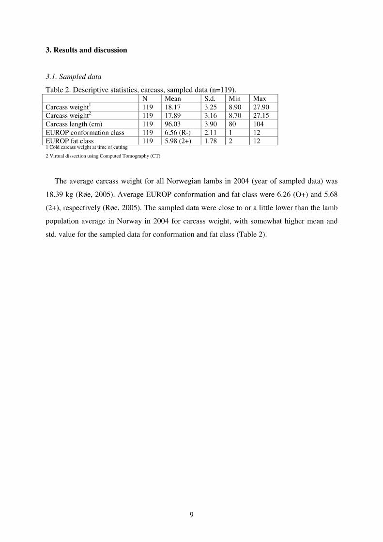
9

3. Results and discussion

3.1. Sampled data

Table 2. Descriptive statistics, carcass, sampled data (n=119). N Mean S.d. Min Max Carcass weight1 119 18.17 3.25 8.90 27.90 Carcass weight2 119 17.89 3.16 8.70 27.15 Carcass length (cm) 119 96.03 3.90 80 104 EUROP conformation class 119 6.56 (R-) 2.11 1 12 EUROP fat class 119 5.98 (2+) 1.78 2 12 1 Cold carcass weight at time of cutting

2 Virtual dissection using Computed Tomography (CT)

The average carcass weight for all Norwegian lambs in 2004 (year of sampled data) was

18.39 kg (Røe, 2005). Average EUROP conformation and fat class were 6.26 (O+) and 5.68

(2+), respectively (Røe, 2005). The sampled data were close to or a little lower than the lamb

population average in Norway in 2004 for carcass weight, with somewhat higher mean and

std. value for the sampled data for conformation and fat class (Table 2).

10

3.2. Precision and reliability of the virtual dissection method using CT scanning on the two

carcass halves. Effect of section distance.

Table 3. Estimated dissection traits yield and carcass tissues fat, muscle and bone for each ½ carcass (n=119 carcasses; 238 halves). Mean value in kg and %, standard deviation (s.d.), absolute side (left-right) difference, coefficient of variation (CV, %) and reliability (REL) correlation coefficient (r) in kg and % for all section distances using sequential scanning (equidistance). Dissection

traits

Mean

(kg)

s.d. Diff

(kg)

CV

(%)

REL Mean

(%)

s.d. Diff

(%)

CV

(%)

REL

½ Carcass weight

8.95 1.58 0.14 1.21 0.99

Fat 0.99 0.40 0.04 3.14 0.99 10.86 3.41 0.30 2.12 0.99 Muscle 6.45 1.17 0.10 1.26 0.99 72.10 2.74 0.56 0.60 0.97

40 mm

Bone 1.51 0.22 0.05 2.62 0.96 17.05 1.83 0.47 2.16 0.95 ½ Carcass weight

8.96 1.60 0.15 1.37 0.99

Fat 1.00 0.40 0.04 3.48 0.99 10.97 3.52 0.38 2.83 0.99 Muscle 6.48 1.22 0.13 1.71 0.99 72.22 3.10 0.91 1.10 0.92

80 mm

Bone 1.49 0.26 0.08 4.49 0.92 16.81 2.62 0.88 4.62 0.90 ½ Carcass weight

0.91 1.66 0.23 2.04 0.99

Fat 1.14 0.46 0.07 4.53 0.99 12.45 3.97 0.63 3.74 0.98 Muscle 6.38 1.25 0.19 2.28 0.99 70.47 4.25 1.41 1.80 0.90

160 mm

Bone 1.53 0.36 0.13 8.73 0.86 17.08 3.49 1.38 7.68 0.85 ½ Carcass weight

8.91 1.96 0.26 2.86 0.98

Fat 1.04 0.45 0.08 8.30 0.97 11.52 3.70 0.79 5.59 0.97 Muscle 6.33 1.43 0.15 8.38 0.87 71.13 4.58 1.58 1.70 0.91

320 mm

Bone 1.53 0.44 0.18 8.38 0.87 17.35 3.72 1.72 7.36 0.83

The precision and reliability of the virtual dissection method was defined by the coefficient

of variation (CV, %) and the correlation (r) between repeated measurements (carcass sides;

left-right), respectively. Table 3 shows the estimated mean value and standard deviation (s.d.)

of the dissection traits, the absolute difference between repeated measurements, the precision

and reliability for section distances (equidistance) from 40 mm to 320 mm using sequential

CT scanning. The carcass side difference increased with increasing equidistance. When using

40 mm section distance, the precision and reliability for ½ carcass weight was 1.21 % and

0.99, respectively. For fat weight and proportions, the precisions and reliabilities were 3.14

and 2.12 %, and 0.99, respectively. For muscle weight and proportions, 1.26 and 0.60 %, and

0.99 and 0.97, respectively. For bone weight and proportions, 2.62 and 2.16 %, and 0.96 and

0.95, respectively. For the other equidistances (80 mm, 160 mm and 320 mm), the precisions

and reliabilities were gradually lower (Table 3) by increasing equidistance.

11

The geometry of fat and muscle tissues was considered to be less irregular compared to

bone (unidirectional) throughout the carcass, i.e. the complex geometry of the rib cage,

having a curved shape which was difficult to model using sequential scanning. This was

especially valid for high section distance (low resolution, 320 mm), where the Cavalieri

estimation was not as precise and reliable compared to lower section distances (40 – 160

mm).

All section distances showed acceptable reliability according to the definition by Nissen et

al. (2006), where reliability above 0.8 was considered an acceptable reference method. For

section distance of 40 mm, the results were excellent, where all reliabilities were above 0.95.

Compared to the precision and reliability of manual dissection presented by Kongsro et al.

(2008), the virtual dissection was both more precise and reliable. For ½ carcass weight, the

results for manual dissection (Kongsro et al., 2008) were 1.56 % and 0.98 for precision and

reliability. For fat, muscle and bone weight, the results were 4.34 % and 0.98, 2.27 and 0.96,

and 4.48 % and 0.85, for precision and reliability, respectively. For fat, muscle and bone

proportion, the results were 4.11 % and 0.93, 1.19 % and 0.80, and 3.00 and 0.90, for

precision and reliability, respectively. For fat and muscle, the results for virtual dissection

using section distances of 40 mm and 80 mm seem to be more precise and reliable compared

to manual dissection. For bone, only the 40 mm section distance seems to be better than

manual dissection.

3.3. Virtual vs. manual dissection

Table 4. Descriptive statistics, manual and virtual dissection (n=119).

Dissection

traits n Mean Std Min Max

Fat (kg) 119 2.45 0.93 0.72 6.34 Muscle (kg) 119 11.07 1.96 5.70 17.56 Bone (kg) 119 3.97 0.58 2.27 5.71 Fat (%) 119 13.23 3.36 8.14 26.09 Muscle (%) 119 61.02 2.75 50.73 67.51 M

anua

l1

Bone (%) 119 22.06 2.05 16.54 25.96 Fat (kg) 119 1.97 0.80 0.44 4.93 Muscle (kg) 119 12.90 2.35 6.44 20.47 Bone (kg) 119 3.02 0.44 1.81 4.34 Fat (%) 119 10.86 3.42 4.20 20.23 Muscle (%) 119 72.10 2.75 65.17 79.39 V

irtu

al2

Bone (%) 119 17.05 1.83 12.74 20.89 1 Manual dissection performed by 5 trained butchers

2 Virtual dissection using Computed Tomography (CT) equidistance 40 mm

12

The correlations between manual and virtual dissection for fat and muscle tissue seemed to

be relatively stable with increasing equidistance, and correlation of bone drops with

increasing equidistance (Figure 3). The most plausible explanation for this phenomenon is the

irregular nature of bone shapes (i.e. complex geometry of rib cage) which is described less

efficiently with greater equidistance. From 40 mm to 160 mm, fat and muscle tissue only

showed minor changes with respect to correlation, which may be indicative that 6 to 7 scans

per lamb carcass or 160 mm is enough to cover variation in total fat and muscle tissue in the

lamb carcasses. For bone, 40 mm or 23 to 27 scans per lamb carcass seemed insufficient to

cover the variation in total bone tissue in lamb carcasses.

The descriptive statistics from the sampled data, both virtual and manual dissection,

showed some differences between the two dissection methods (Table 4). The amount of

muscle tissue was higher for virtual dissection both in kg and %, compared to manual

dissection. This may be due to that manual dissection underestimates the muscle content by

leaving too much meat on bones and the sorting of manufacturing meat by fat content

(Kongsro et al. 2008). The Cavalieri estimation overestimates muscle content by extrapolating

the void between section distances using section images, where the bone structure is not

completely covered, compromising bone and replacing the void with muscle. The difference

in carcass weight between carcass weighing and virtual dissection (Table 2) may also be the

results of underestimation of bone and overestimation of muscle. Bone has higher density

than muscle, and the carcass weight will therefore be somewhat lower when muscle is

overestimated. The amount of fat was smaller compared to manual dissection, both in kg and

%. The reason for this difference may be due to the practise of sorting meat into manufactured

meat. The inaccuracy of butchers separating fat from lean muscle was reflected in the work by

Kongsro et al. (2008). There may also be an effect of Cavalieri estimation, where fat depots

are not well modelled or extrapolated.

13

40 mm 80 mm 160 mm 360 mm0.4

0.5

0.6

0.7

0.8

0.9

1

Equidistance

Co

rrela

tio

n (

r)

Fat (kg)

Muscle (kg)

Bone (kg)

Fat (%)

Muscle (%)

Bone (%)

Figure 3. Correlation between manual dissection and virtual (CT) dissection (equidistance 40, 80, 160 and 320 mm).

The relationship between true carcass weight and CT estimated carcass weight is shown in

Figure 4. Virtual dissection with 40 mm equidistance is used for comparison with manual

dissection and true carcass weight. The correlation is very high (r=0.99) and there is only a

minor bias (difference between red target line (Y=X) and blue predicted line) for large

carcasses, where carcass weight is slightly underestimated. This underestimation is reflected

in the descriptive statistics, and may be the results of Cavalieri estimation, overestimating

muscle at the sacrifice of bone (higher density).

14

5 10 15 20 25 305

10

15

20

25

30

CCW (kg)

CT

(kg

)

Figure 4. Relationship between true carcass weight (kg) and CT carcass estimated carcass weight (kg).

For manual vs. virtual dissection, the correlation of fat in kg is good (r=0.90) (Figure 5).

There is some bias for fat in kg, where fat is underestimated; i.e. for 5 kg dissected fat, the

difference is approx. 1 kg (4 kg for virtually dissected fat).

0 1 2 3 4 5 6 70

1

2

3

4

5

6

7

Dissected fat (kg)

CT

fa

t (k

g)

Figure 5. Relationship between manual dissected fat (kg) and CT carcass estimated fat (kg).

For muscle in kg, the correlation (r=0.98) is higher than for fat (Figure 6), but the bias and

drift from red target line is the opposite from fat; muscle in kg is overestimated and the

overestimation increases with increasing amount of muscle in kg; i. e. 12 kg of dissected

muscle corresponds to 14 kg of virtual dissected muscle.

15

4 6 8 10 12 14 16 18 20 224

6

8

10

12

14

16

18

20

22

Dissected muscle (kg)

CT

muscle

(kg)

Figure 6. Relationship between manual dissected muscle (kg) and CT carcass estimated muscle (kg).

For bone in kg, the relationship is good (r=0.92) (Figure 7), but there is a large drift and

bias from the red target line where bone is highly underestimated, i. e. 4 kg of dissected bone

corresponds to 3 kg of virtually dissected bone.

1 2 3 4 5 61

2

3

4

5

6

Dissected bone (kg)

CT

bon

e (

kg

)

Figure 7. Relationship between manual dissected bone (kg) and CT carcass estimated bone (kg).

The bias and drift from target line Y=X were reflected in Table 4, where differences in

manual and virtual dissection are shown. The standard deviations (s.d.) between the different

16

dissection methods are almost identical, however, the std. for muscle tissue in kg, seemed to

be somewhat larger for virtual dissection. The butchers seem to shrink the scale of muscle

tissue, due to poorer separation of muscle, fat and bone tissue. For bone, the std. seems to be

somewhat larger for manual dissection, which may be a direct result of the combination

between the assumptions used in virtual dissection, and muscle residue left on bone by the

butchers. Adjustment of tissue thresholds within reasonable limits using the peaks and valleys

in Figure 2 was tested to reduce the bias between manual and virtual dissection. The tissue

estimates or the bias did not change significantly when adjusting thresholds back and forth for

all tissues, indicating that the thresholds are robust, flexible and inelastic. Another reason for

the bias in fat, muscle and bone between the two dissection methods may be the scanning

method, where the section distance using sequential scanning is not accurate enough to detect

the variation in tissues, especially for bone shape and size. The underestimation of bone using

Cavalieri estimation of the void between the sections has an effect on the estimation of the

other tissues and the volume and mass of the entire object (lamb carcass). The solution for

this problem is to scan with smaller section distances (< 40 mm) or use spiral scanning. With

new CT scanners, spiral scanning is part of the standard operating protocol, and will probably

be the fastest and best option available. The bias between manual and virtual dissection

seemed to be a sum of two sources of error; butcher and Cavalieri estimation, where the

Cavalieri estimation error increases with increasing section distance.

Formulas for tissue density, like the one used by Campbell et al. (2003) for estimation of

tissue density, have been suggested to be instrument dependent (Håseth et al., 2007).

Differences between CT scanners or units must be accounted for by testing the validity of the

tissue density formula. Such test was not performed in this study; however, it is recommended

in future studies.

17

4. Conclusion and application

Virtual dissection using sequential scanning in this study has proved to be an alternative to

manual dissection, despite some bias between manual and virtual ones. The high values for

the correlations suggest that prediction of fat, lean and bone would be accurate using CT.

It is assumed that the butchers cannot cut with the same accuracy as CT, and this needs to

be accounted for in the virtual value assessment. The precision of virtual dissection in this

study was higher compared to manual dissection and was highest with dense sequential

scanning (40 mm), and lower with increasing equidistance (80 to 320 mm). Complex bone

structures and irregular 3D structures could have led to some bias between virtual and manual

dissection, especially for bone, which was highly underestimated. The bias in carcass tissue

seems to be a combination of inaccurate butcher dissection and overestimation of muscle

tissue by Cavalieri estimation and sequential scanning for virtual dissection. By correcting for

bias and assessing size of butcher error, virtual dissection can be put into practical use.

Introducing spiral scanning or reducing sequential section distance, to cover the more

variation in irregular components of the skeleton and reducing void between sections, may

also prove advantageous.

Acknowledgements

This study was sponsored by grant 162188 of the Research Council of Norway, as part of a

Ph.D. study program. Engineer Knut Dalen is acknowledged for operating the CT Scanner at

UMB, Ås and for valuable discussions that has contributed to this paper. The pilot plant

butchers at Animalia are acknowledged for their practical skills and knowledge.

18

References

Campbell, A. W., Bain, W. E., McRae, A. F., Broad, T. E., Johnstone, P. D., Dodds, K. G.,

Veenvliet, B. A., Greer, G. J., Glass, B. C., Beattie, A. E., Jopson, N. B., & McEwan, J. C.

(2003). Bone density in sheep: genetic variation and quantitative trait loci localisation. Bone,

33, 540-548,

Dobrowolski, A., Branscheid, W., Romvari, R., Horn, P., & Allen, P. (2004). X-ray computed

tomography as possible reference for the pig carcass evaluation. Fleischwirtschaft, 84, 109-

112.

Gundersen, H. J. G, Korbo, T. F., Marcussen, N., Møller, A., Nielsen, K., Nyengaard, J. R.,

Pakkenberg, B., Sørensen, F. B., Vesterby, A., and West, M. J., (1988). Some new, simple

and efficient stereological methods and their use in pathological research and diagnostics.

Acta Pathol.Microbiol.Immunol.Scand., 96, 379-394,

Håseth, T. T., Egelandsdal, B., Bjerke, F. & Sørheim, O. (2007). Computed Tomography for

Quantitative Determination of Sodium Chloride in Ground Pork and Dry-Cured Hams,

Journal of Food Science, 72, 8, Page E420

Johansen, J., Aastveit, A. H., Egelandsdal, B., Kvaal, K. & Roe, M. (2006). Validation of the

EUROP system for lamb classification in Norway; repeatability and accuracy of visual

assessment and prediction of lamb carcass composition. Meat Science, 74, 497-509.

Johansen, J., Egelandsdal, B., Roe, M., Kvaal, K., & Aastveit, A. H. (2007). Calibration

models for lamb carcass composition analysis using Computerized Tomography (CT)

imaging. Chemometrics and Intelligent Laboratory Systems, 87, 303-311.

Jones, H. E., Lewis, R. M., Young, M. J., & Wolf, B. T. (2002). The use of X-ray computer

tomography for measuring the muscularity of live sheep. Animal Science, 75, 387-399.

19

Jopson, N.B., Kolstad, K., Sehested, E., & Vangen, O. (1995). Computer tomography as an

accurate and cost effective alternative to carcass dissection. Australian Association of Animal

Breeding and Genetics. Proceedings, vol. 11, 635-638.

Kalender, W. A. (2005). Computed Tomography - Fundamentals, System Technology, Image

Quality, Applications. 2nd revised edition. Wiley-VCH; 2 Har/Cdr edition.

Kongsro, J., Egelandsdal, B., Kvaal, K., Røe, M., & Aastveit, A.H. (2008). The reference

butcher panel’s precision and reliability of dissection for calibration of lamb carcass

classification in Norway. Animal, Submitted.

Kvame, T. & Vangen, O. (2007). Selection for lean weight based on ultrasound and CT in a

meat line of sheep. Livestock Science, 106, 232-242.

Lambe, N. R., Conington, J., Mclean, K. A., Navajas, E. A., Fisher, A. V., & Bunger, L.

(2006). In vivo prediction of internal fat weight in Scottish Blackface lambs, using computer

tomography. Journal of Animal Breeding and Genetics, 123, 105-113.

Lambe, N. R., Young, M. J., Mclean, K. A., Conington, J., & Simm, G. (2003). Prediction of

total body tissue weights in Scottish Blackface ewes using computed tomography scanning.

Animal Science, 76, 191-197.

Lambe, N. R., Navajas, E. A., Mclean, K. A., Simm, G., & Bunger, L. (2007). Changes in

carcass traits during growth in lambs of two contrasting breeds, measured using computer

tomography. Livestock Science, 107, 37-52.

Navajas, E. A., Lambe, N. R., Mclean, K. A., Glasbey, C. A., Fisher, A. V., Charteris, A. J.

L., Bunger, L., & Simm, G. (2007). Accuracy of in vivo muscularity indices measured by

computed tomography and their association with carcass quality in lambs. Meat Science, 75,

533-542.

Navajas, E. A., Lambe, N. R., Mclean, K. A., Glasbey, C. A., Fisher, A. V., Charteris, A. J.

L., Bunger, L., & Simm, G. (2007). Accuracy of in vivo muscularity indices measured by

20

computed tomography and their association with carcass quality in lambs. Meat Science, 75,

533-542.

Nissen, P. M., Busk, H., Oksama, M., Seynaeve, M., Gispert, M., Walstra, P., Hansson, I., &

Olsen, E. (2006). The estimated accuracy of the EU reference dissection method for pig

carcass classification. Meat Science, 73, 22-28.

Roberts, N., Cruzorive, L. M., Reid, N. M. K., Brodie, D. A., Bourne, M., & Edwards, R. H.

T. (1993). Unbiased Estimation of Human-Body Composition by the Cavalieri Method Using

Magnetic-Resonance-Imaging. Journal of Microscopy, 171, 239-253.

Romvari, R., Dobrowolski, A., Repa, I., Allen, P., Olsen, E., Szabo, A., & Horn, P., (2006).

Development of a computed tomographic calibration method for the determination of lean

meat content in pig carcasses. Acta Veterinaria Hungarica, 54, 1-10.

Røe, M. (2005). Annual report: classification and weight results for 2004, Norway.

Norwegian Meat Research Centre. Internal report available animalia@animalia.no.

Sehested, E. (1986). In-vivo prediction of lamb carcass composition by computerized

tomography. Ph.D. Thesis, Agricultural University of Norway.

Szabo, C., Babinszky, L., Verstegen, M. W. A., Vangen, O., Jansman, A. J. M., & Kanis, E.,

(1999). The application of digital imaging techniques in the in vivo estimation of the body

composition of pigs: a review. Livestock Production Science, 60, 1-11.

Skjervold, H., Gronseth, K., Vangen, O., & Evensen, A. (1981). In vivo estimation of body

composition by computerised tomography. Zeitschrift für Tierzüchtung und

Züchtungsbiologie, 98, no. 183, 77–79.

Standal, N. (1984). Establishment of CT facility for farm animals. In Vivo Measurement of

Body Composition in Meat Animals, Lister, D. (Ed.), Elsevier, London, pp. 43–51.

21

Thompson J. and Kinghorn B. (1992). CATMAN - A program to measure CAT-Scans for

prediction of body composition in live animals. Australian Association of Animal Breeding

and Genetics. 10:560-564

Paper V

1

Prediction of fat, muscle and value in Norwegian lamb carcasses using EUROP

classification, carcass shape and length measurements, visible light reflectance

and computer tomography (CT)

J. Kongsroa,b*, M. Røea, K. Kvaalc, A.H. Aastveitb and B. Egelandsdalb

a Animalia – Norwegian Meat Research Centre, P.O. Box 396 Økern, N-0513 Oslo, Norway

b Dept. of Chemistry, Biotechnology and Food Science, Norwegian University of Life Sciences, P.O. Box 5003, N-1432 Ås, Norway

c Dept of Mathematical Sciences and Technology, Norwegian University of Life Sciences, P.O. Box 5003, N-1432 Ås, Norway

Abstract

84 carcasses were sampled to compare different techniques or methods for prediction of

lamb carcass composition and value. Four methods that are used at the Norwegian Meat

Research Centre, Animalia, were selected. These were basic EUROP classification, advanced

EUROP classification using carcass shape and length measurements, visible light reflectance

probing (GP) and Computer Tomography (CT). Multivariate Calibration models were

developed for all techniques against dissected fat and muscle, carcass value and carcass value

per kg. The calibration models were validated using a separate test set of 36 sampled

carcasses. The best prediction models were obtained using CT, with respect to explained

variance, prediction error and bias. Basic EUROP classification seemed to be the most biased

technique of the four types selected in this trial. EUROP assessors seemed to underestimate

large carcasses, especially with respect to muscle in kg and carcass value. Due to high cost

and low operating speeds of CT, optical probing (GP) may be the second best solution of the

technologies used in this study, combined with a CT dissection reference as an alternative to

manual dissection.

Keywords: Lamb, carcass composition, prediction, multivariate calibration, computer tomography, visible light reflectance, probing, EUROP

classification, carcass shape and length measurements

* Corresponding author. Phone: +4722092246; Fax: +4722220016.

E-mail address: jorgen.kongsro@animalia.no (Jørgen Kongsro)

2

1. Introduction

A number of different technologies for measuring composition of carcasses on-line

(automated sampling or analysis) exists, i.e. visual classification, linear measurements using

human or computer vision, visual, IR or NIR reflectance, conductivity, bio-impedance and

computer tomography (CT). The most common technology used in the meat industry is visual

classification, either by use of the EUROP (Europe) or the USDA classification system (North

America). Lamb production in Norway, and in many countries worldwide, is based on season

slaughter, where a large number of animals are slaughtered during a limited period of time

during autumn. Season-based slaughter presents a challenge with respect to on-line

measurements of carcasses. The first challenge is speed, where a large number of carcasses

pass through the abattoirs during slaughter. The second challenge is calibration and

repeatability, where it is difficult for operators to be accurate from year to year when the

assessment is carried out during a short period each year.

Accurate assessments and prediction of carcass tissue and value are of great importance for

suppliers of meat to consumers. In a review by Stanford et al. (1998) of methods for

predicting lamb carcass composition, a large set of in and ex vivo methods for prediction of

lamb carcass composition based on previous published or unpublished trials are described, but

they did not do a comparison of methods based on real data. This study compares a smaller

set of ex vivo methods using real data for comparison. In Norway and the rest of Europe, the

carcass classification system, EUROP is used on-line, and is practiced by trained operators or

classifiers by visual appraisal (Johansen et al., 2006). Their evaluation time is relatively short

(5 to 10 seconds), but the accuracy has proven to be poor, especially for carcass muscle

content and value (Johansen et al., 2006). An advanced version of the EUROP system

(Commission Regulation (EC) No 823/98, 1998; Commission Regulation (EEC) No 461/93,

1993), which is used by national inspectors (Johansen et al., 2006) make use of specific

carcass shape and length measurements, and is regarded to be more accurate, but the

evaluation time is higher than the standard EUROP procedure. Grading probes using visible

light reflectance are used in the meat industry for pig carcasses in Norway, but is not currently

used for lambs or sheep. The evaluation time is fast, and a trained operator only needs 5

seconds for carcass evaluation. The accuracy of probes is acceptable, especially for pig

carcasses, but the subcutaneous fat is more difficult to assess for lamb and sheep compared to

pig, due to the lack of rind to support the probe and more heterogeneous distribution of fat in

lamb and sheep carcasses. Pigs have a higher percentage of body subcutaneous fat compared

3

to ruminants such as sheep and cattle. Recent versions of grading probes can also assess meat

quality, i.e. marbling, colour and water-holding capacity. Computer Tomography (CT) has

been shown to hold great potential for early and accurate assessment, both for live animal and

carcass fatness, muscularity and weight (Cross and Belk, 1994; Kvame et al., 2004; Lambe et

al., 2003; Macfarlane et al., 2004; Macfarlane et al., 2006; Stanford et al., 1998). However,

CT is regarded as an expensive tool and the carcass evaluation time required is somewhat

higher than that of other on-line methods. Recent advances on development of CT scanners

have introduced multi-slice scanning combined with spiral scanning that have achieved

speeds from 4 to 16 images per second (Lewis et al., 2006). With this speed, carcasses can be

evaluated and assessed according to carcass composition at chain speed, on-line in abattoirs.

The repeatability, reproducibility and reliability of visual classification using EUROP

classification are found to be good (Johansen et al. 2006) using classes to classify carcasses,

however, there were some bias between the Commission standards assessed by National

assessors and industry assessors. The operators are consistent; however, the system has

proven to predict carcass composition poorly, especially for lean meat or muscle content. For

visible light reflectance using probes, a number of factors influencing the accuracy in addition

to calibration were reported by (Fisher, 1997; Olsen et al., 2007). These include maintenance

of instruments, training of operators and working conditions. The authors found that the

variations between operators were more important than variations between the probe

instruments from different manufacturers. For CT, the results from Johansen et al. (2007)

showed that CT was a useful tool for predicting fat and muscle tissues in lamb carcasses.

The most common reference method used for calibration of technologies for carcass

composition is carcass dissection. For visual classification like EUROP (Johansen et al. 2006;

(Commission Regulation (EC) No 823/98, 1998; Commission Regulation (EEC) No 461/93,

1993) and USDA classification (Fisher, 1997; Olsen et al., 2007; USDA, 1992), regulations

between or within countries for carcass conformation class and fat class are determined and

used as reference method. The visual classification methods are most often supervised by

national assessors using the regulations as reference method (Johansen et al. 2006). Dissection

has proven to be accurate for lean meat content in pig carcasses (Nissen et al., 2006), but

somewhat poorer with respect to repeatability and reliability with respect to fat and muscle

(lean meat) for lamb carcasses (Johansen et al., 2007). New reference methods using

Computer Tomography (CT) has proven to be more accurate, faster and more cost-effective

for estimating lamb carcass composition (Kongsro et al., 2008). The results showed that CT

was more precise and reliable compared to manual dissection, however there were some

4

biases between manual and CT dissection, especially for estimation of bone, which could be

explained by butcher and CT estimation error.

The main objective of this study was to compare the accuracy and prediction of carcass

soft tissues (fat and muscle) weights and carcass value using different on-line technologies for

lamb carcasses; EUROP, advanced EUROP using linear measurements, visible light grading

probe and computer tomography (CT).

2. Materials and methods

2.1 Experimental data

One hundred and twenty (120) lambs from a single Norwegian abattoir were sampled

during autumn of 2005. The experimental design was set up to cover the variation in all levels

of fatness in the carcasses based on the principle of over-sampling at the extremes (Engel et

al., 2003; Johansen et al., 2007b). The carcasses were sampled in three groups; low,

intermediate and high level of fatness (Johansen et al., 2007b). The data was split into two

sets; calibration (84 samples) and test sets (36 samples).

2.2 EUROP classification

The lamb carcasses were classified using the European system EUROP, according to

conformation and fat group (Johansen et al., 2006). In this study, the EUROP classification

system was assessed by trained National assessors in a cool storage room at Animalia pilot

plant. This was done to ensure the best possible accuracy and repeatability of measurements.

2.3. EUROP advanced – carcass shape and length measurements

In addition to ordinary EUROP classification and carcass weight, several carcass shape and

length measurements were sampled from the carcasses (Fig. 1). These measurements were

sampled by Animalia assessors using manual rulers. The measurements were based on the

detailed rules laid down by the EU commission concerning the classification of ovine animals

(Commission Regulation (EEC) No 461/93, 1993).

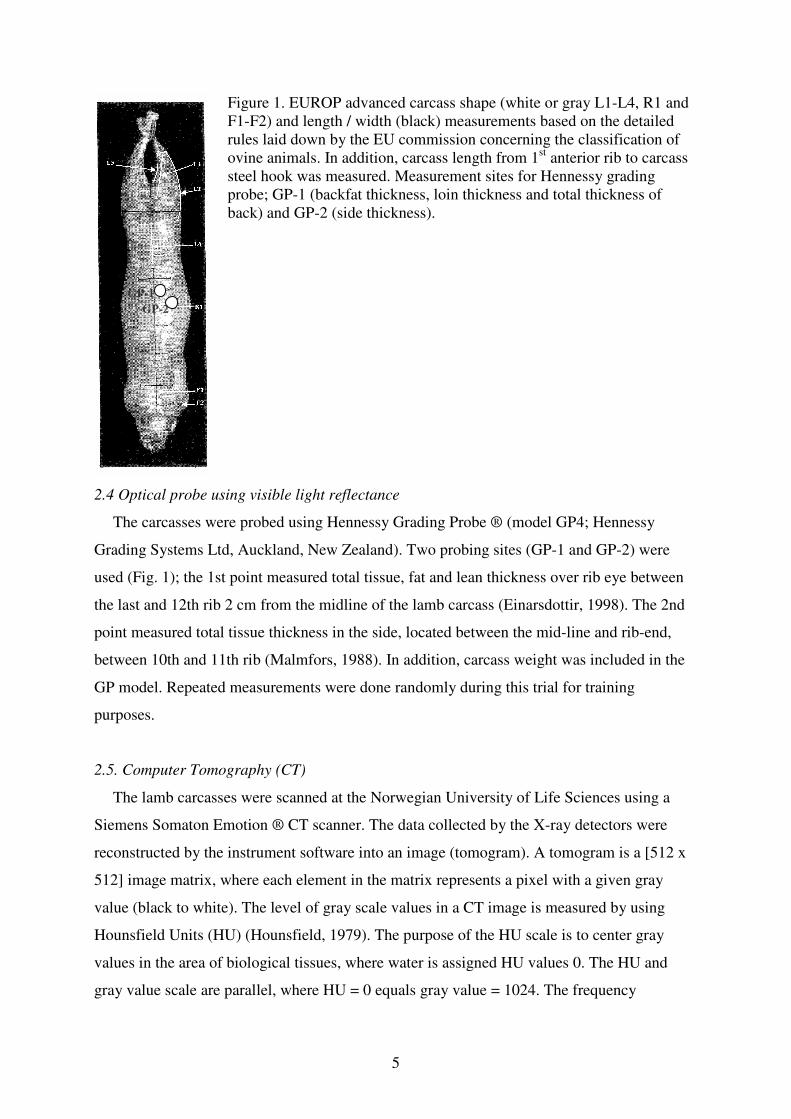
5

Figure 1. EUROP advanced carcass shape (white or gray L1-L4, R1 and F1-F2) and length / width (black) measurements based on the detailed rules laid down by the EU commission concerning the classification of ovine animals. In addition, carcass length from 1st anterior rib to carcass steel hook was measured. Measurement sites for Hennessy grading probe; GP-1 (backfat thickness, loin thickness and total thickness of back) and GP-2 (side thickness).

2.4 Optical probe using visible light reflectance

The carcasses were probed using Hennessy Grading Probe ® (model GP4; Hennessy

Grading Systems Ltd, Auckland, New Zealand). Two probing sites (GP-1 and GP-2) were

used (Fig. 1); the 1st point measured total tissue, fat and lean thickness over rib eye between

the last and 12th rib 2 cm from the midline of the lamb carcass (Einarsdottir, 1998). The 2nd

point measured total tissue thickness in the side, located between the mid-line and rib-end,

between 10th and 11th rib (Malmfors, 1988). In addition, carcass weight was included in the

GP model. Repeated measurements were done randomly during this trial for training

purposes.

2.5. Computer Tomography (CT)

The lamb carcasses were scanned at the Norwegian University of Life Sciences using a

Siemens Somaton Emotion ® CT scanner. The data collected by the X-ray detectors were

reconstructed by the instrument software into an image (tomogram). A tomogram is a [512 x

512] image matrix, where each element in the matrix represents a pixel with a given gray

value (black to white). The level of gray scale values in a CT image is measured by using

Hounsfield Units (HU) (Hounsfield, 1979). The purpose of the HU scale is to center gray

values in the area of biological tissues, where water is assigned HU values 0. The HU and

gray value scale are parallel, where HU = 0 equals gray value = 1024. The frequency

GP-1

GP-2

6

distributions of pixel HU values (histogram) for were used for calibration (X-data), yielding

2280 gray level values from black (0) to white (2280). 15 anatomical scans were taken across

the entire carcass (Johansen et al., 2007), and the histograms of HU values were generated for

the sum of pixels from all anatomical sites.

2.6. Commercial dissection, end point reference (Y)

A team of 5 highly skilled butchers at Animalia (Norwegian Meat Research Centre) pilot

plant dissected the 120 lamb carcasses. Whole carcasses from lambs were commercially

dissected according to Norwegian Meat Industry commercial standards (Johansen et al.,

2006). The carcasses were cut into five major cuts: leg, loin, side, shoulder and breast. Each

of the major cuts was separated and sorted into fat, muscle and bone tissue, and the mass (kg)

of the different tissues were estimated for the entire carcass. Dissected fat (kg), muscle (kg)

and value in NOK (Norwegian kroner) and NOK / kg was used as end point reference (Y-

vector) for calibration. The reference prices for the major cuts are retrieved from Norway

Meat commercial industry prices for lamb cuts in autumn of 2006. The currency was

approximately 1 EUR = 8 NOK (Oct. 2007).

2.7. Statistical data analysis – modelling

2.7.1. Multivariate calibration

All calibration models were constructed using a calibration set of 84 samples (Tab. 1).

The EUROP data matrix contained EUROP conformation, fat class and carcass weight. The

EUROP advanced data matrix contained linear measurements, EUROP conformation and fat

class, and carcass weight. The optical probe data matrix contained GP fat cover (GP-1), GP

muscle thickness (GP-1), GP total thickness (GP-1), GP side thickness (GP-2) and carcass

weight. The CT data matrix contained the frequency distribution (histograms) of HU values

range from [-200,200] (Johansen et al., 2007) in addition to carcass weight. The data for the

different models were mean-centered and scaled using the autoscale option in PLS_Toolbox

4.1, Copyright 2006 Eigenvector Research, Inc. for use with MATLAB R2007a, Version

7.4.0.287 (R2007a), Copyright 1984-2007, The Mathworks, Inc. All the data matrices were

calibrated against the end-point reference Y (dissected fat and muscle (kg) and value in NOK

and NOK/kg). The calibration models were constructed using Partial Least Square Regression

(PLSR) (Martens and Martens, 2001) and were modelled using PLS_Toolbox function

analysis. The calibration models were validated using full leave-one-out cross-validation. The

optimal number of PLS components in the calibration models were decided seeking the

7

lowest Root Mean Square Error of Cross-Validation (RMSECV) (Esbensen, 2000). RMSECV

is regarded as a measure of model quality, and is defined by:

∑=

−=n

i

i

cv

i yyn

RMSECV1

2)ˆ(1

(1)

where n is the number of samples in the calibration set, the i

y ’s are the real (measured)

responses and the i

y ’s are the estimated responses found via cross-validation (Cederkvist et al., 2005).

During multivariate calibration, important predictors in each model were found using the

PLS_Toolbox 4.1, Variable Importance in Projection (VIP) (Chong and Jun, 2005). VIP

estimates the importance of each variable used in a PLS model. A variable with VIP score

larger than 1 can be considered to be important in a given model.

2.7.2. Prediction

When the performance of the calibration set was tested and the optimal number of latent

components using RMSECV was found, the predictive ability of the calibration models was

validated using a test set. The test set validation was applied using Root Mean Square Error of

Prediction (RMSEP) and systematic errors in predictive values (BIAS):

∑=

−=n

i

i

p

i yyn

RMSEP1

2)ˆ(1

(2)

where n is the number of samples in the test set, the yi’s are the real (measured) responses and

the i

y ’s are the estimated responses found via cross-validation:

)ˆ(1

1i

p

i

n

i

yyn

BIAS −= ∑=

(3)

where n is the number of samples in the calibration set, the i

y ’s are the real (measured)

responses and the i

y ’s are the estimated responses found via cross-validation.

8

3. Results

Table 1. Mean values and variation of different carcass traits measurements on lamb carcasses. Calibration and validation (test) set. Carcass traits Mean1 Std1 Mean2 Std2

Weight (kg) 18.49 5.48 19.09 5.28 Fat (kg) 3.27 2.19 3.51 2.23 Muscle (kg) 10.35 2.77 10.95 2.59 EUROP Conformation class 6.33 (O+) 3.48 6.28 (O+) 3.13 EUROP Fat class 6.40 (2+) 3.64 6.47 (2+) 3.32 HGP fat thickness loin (GP-1) 45.63 33.51 51.11 36.37 HGP muscle thickness loin (GP-1) 287.20 100.53 302.11 90.61 HGP total thickness loin (GP-1) 419.18 95.15 439.97 81.71 HGP side thickness (GP-2) 147.45 72.63 156.22 67.71 Value (NOK3) 893.72 287.01 953.64 283.24 Value (NOK3/kg) 49.75 1.79 50.17 1.98 1 Calibration set (n=84)

2. Validation (test) set (n=36)

3 1 NOK = 0.126 EUR

In Table 1, the mean value and variation of the measurements applied on the carcasses are

shown. The carcass weight in kg is close to the national mean value (18.39 kg) of Norwegian

lamb carcasses in 2004 (Røe, 2005), both for the calibration and validation (test) set. For

conformation and fat class, the mean value was close to national mean (6.26) for

conformation class, and somewhat higher than national mean (5.68) for fat class. The larger

value for fat class is due to the set up of experimental design, spanning the variation of fatness

in carcasses.

Table 2. Prediction of fat (kg). Number of components (#) in PLS model, explained variance calibration (R2

cal), calibration error using cross-validation (RMSECV), explained variance prediction (R2

pred), prediction error using test set validation (RMSEP), bias and most important variable in projection (VIP). # R

2cal RMSECV R

2pred RMSEP Bias VIP

EUROP1 2 0.697 1.200 0.620 1.373 -0.191 Fat class

EUROP2

ADV

4 0.755 1.080 0.588 1.421 -0.109 Fat class

GP3 5 0.876 0.767 0.904 0.694 0.055 GP side

CT4 3 0.922 0.614 0.935 0.571 0.085 HU value -63

1 Basic EUROP

2 Advanced EUROP; carcass shape and length measurements

3 Visible light reflectance; Hennessy Grading Probe

4 Computer Tomography

The prediction of fat in kg is shown in Table 2. Only a small difference in prediction of fat

(kg) was found between basic and advanced EUROP classification. The calibration results

9

(RMSECV) was slightly better for EUROP advanced. EUROP advanced was also less biased

compared to basic EUROP. The most important predictor was EUROP fat class. The R2

values were 0.62 and 0.59 for basic and advanced EUROP, and the prediction error were 1.37

and 1.42, respectively. GP and computer tomography (CT) both achieved R2 values larger

than 0.9, with prediction error of 0.69 and 0.57, respectively. The most important predictor

(VIP) for fat (kg) for GP was GP side (side thickness), and the most important CT value was

HU = -63. Basic EUROP seemed to be slightly more biased (-0.19) compared to GP and CT

(0.05 and 0.08, respectively).

Table 3. Prediction of muscle (kg). Number of components (#) in PLS model, explained variance calibration (R2

cal), calibration error using cross-validation (RMSECV), explained variance prediction (R2

pred), prediction error using test set validation (RMSEP), bias and most important variable in projection (VIP). # R

2cal RMSECV R

2pred RMSEP Bias VIP

EUROP1 1 0.634 1.669 0.699 1.499 -0.516 Carcass weight

EUROP2

ADV

2 0.754 1.618 0.712 1.384 -0.151 L1

GP3 1 0.733 1.425 0.690 1.432 -0.164 Carcass weight

CT4 5 0.910 0.833 0.917 0.744 0.007 HU value 63

1 Basic EUROP

2 Advanced EUROP; carcass shape and length measurements

3 Visible light reflectance; Hennessy Grading Probe

4 Computer Tomography

The prediction of muscle (kg) is shown in Table 3. EUROP advanced seemed to perform

slightly better compared to basic EUROP, with R2 values of 0.70 and 0.71, and RMSEP

values of 1.50 and 1.38 for basic and advanced EUROP, respectively. Carcass weight and

linear measure L1 (circumference of m. semimembranosus) (Fig. 1), seemed to be the best

predictors for basic and advanced EUROP, respectively. GP did not improve the predictions

of muscle compared to EUROP, while CT showed major improvements, yielding a R2 value

of 0.92 and prediction error of 0.74. The most important predictors for GP and CT was

carcass weight and CT value HU = 63. Basic EUROP (-0.516) seem to be more biased than

the other methods, and seem to underestimate the muscle content in kg, especially for

carcasses with high content of muscle in kg. CT gave the smallest bias, and seems to be

virtually unbiased with respect to muscle in kg (0.007). The comparison of different methods

for prediction of muscle (kg) is shown in Figure 2.

10

4 6 8 10 12 14 16 184

6

8

10

12

14

16

18

Predicted muscle (kg)

Measure

d m

uscle

(kg)

dis

section

EUROP

EUROPADV

GP

CT

Figure 2. Measured vs. predicted; muscle (kg). Measurements: EUROP, EUROP advanced, Hennessy Grading Probe (GP) and computer tomography (CT). Table 4. Prediction of value (NOK). Number of components (#) in PLS model, explained variance calibration (R2

cal), calibration error using cross-validation (RMSECV), explained variance prediction (R2

pred), prediction error using test set validation (RMSEP), bias and most important variable in projection (VIP). # R

2cal RMSECV R

2pred RMSEP Bias VIP

EUROP1 1 0.728 148.850 0.727 155.250 -49.976 Carcass weight

EUROP2

ADV

3 0.831 117.390 0.736 144.770 -18.846 L1

GP3 2 0.833 116.720 0.830 116.460 -14.943 GP side

thickness CT

4 5 0.940 70.130 0.945 65.420 -0.660 HU value 63 Table 5. Prediction of value (NOK/kg). # R

2cal RMSECV R

2pred RMSEP Bias VIP

EUROP1 1 0.001 1.797 0.039 1.961 -0.402 Carcass weight

EUROP2

ADV

1 0.004 1.794 0.048 1.949 -0.379 Width of leg

GP3 1 0.027 1.766 0.103 1.892 -0.319 GP total loin

thickness CT

4 3 0.196 1.607 0.396 1.530 -0.173 HU value 70 1 Basic EUROP

2 Advanced EUROP; carcass shape and length measurements

3 Visible light reflectance; Hennessy Grading Probe

4 Computer Tomography

The predictions of value in NOK and NOK/kg are shown in Table 4 and 5. Basic EUROP

seemed to yield somewhat poorer predictions compared to advanced EUROP. Basic EUROP

11

seemed to be more biased than the other methods. The most important predictor for value in

NOK was carcass weight and linear measure L1 (Fig. 1), for basic and advanced EUROP,

respectively. For value in NOK/kg, the most important predictors were carcass weight and

width of leg (Fig. 1), for basic and advanced EUROP, respectively. GP and CT seemed to

improve the predictions, with CT yielding the highest R2 values and lowest RMSEP. The

most important predictors for GP and CT for value in NOK were GP side and CT value

HU=63. For value in NOK / kg, HGP total and CT value HU 70 were the most important

predictors. The variance explained for value in NOK / kg was low for all methods, not

achieving R2 values above 0.4 for prediction. CT gave the lowest bias of all the methods, -

0.66 and -0.17 for value in NOK and NOK / kg, respectively.

4. Discussion

All data in this study have been sampled in controlled environments. In an industry

environment, it is highly probable that the accuracy of measurements will be poorer due to

faster operating speed and other influential factors during production. These factors may be

handled by automating measurements, making them less vulnerable to human assessment or

operator error. EUROP and carcass shape and length measurements can be automated by

image analysis such as video image analysis or VIA. GP can be automated by using robotics

for probing to ensure high repeatability. CT is already an equipment-driven application, and

may be automated by computer programming and feeding carcasses into the CT during

slaughter. The speed and cost of CT is, however, still a major concern for industry

applications.

For prediction of fat tissue, the results showed that GP and CT predicted fat tissue well

achieving R2 higher than 0.9. EUROP predicted fat somewhat satisfactory, and the most

important predictor was EUROP fat class. The most important GP predictor was side

thickness (GP side), which indicates that side thickness of lamb carcasses is a very good

predictor of carcass fat. Previous studies of CT value frequency distribution (histogram)

showed that the CT histograms of lamb carcass soft tissues had two peaks, separated by a

valley; the left peak represented the amount of fat, and the right peak amount of muscle

(Johansen et al. 2007). The CT value HU=-63, which was the most important predictor for fat,

represented the local maxima of the left peak in CT histogram. In relation to cost and speed,

the results for GP showed that this method is very promising for prediction of carcass fat,

which was in accordance with the previous studies by Johansen et al. (2007) and Kongsro et

12

al. (2008). Side thickness measured by GP seemed to be a very good predictor of carcass

fatness.

For prediction of muscle, CT predicted muscle in kg well, achieving R2 higher than 0.9.

The other methods predicted muscle satisfactorily, whereas advanced EUROP using linear

measurements achieved the highest explained variance. Conformation does not seem to

contribute more to explaining variation in muscle (kg) compared to carcass weight using basic

EUROP, which indicates the importance of carcass weight as a single predictor for muscle.

Carcass weight is also objective and cheap for on-line use. If repeatability, reproducibility and

reliability of EUROP classification are poor, one can consider the use of carcass weight as a

single predictor of carcass muscle. The L1 measure (circumference of m. semimembranosus)

was the most important predictor of muscle using advanced EUROP, but carcass weight was

almost similar with respect to VIP measures. The circumference of m. semimembranosus

seemed to be a good indicator of muscle content in carcasses. Carcass weight was also the

most important predictor for GP measures, but the probe measurements (GP-1 and GP-2)

seemed to add some explained variation to the models compared to basic EUROP

classification. During this trial, there were some challenges using GP measurements in the

loin; site GP-1 (Fig. 1). For very small carcasses, it was especially difficult to probe the

muscle perpendicularly, and the accuracy and repeatability may be affected. By using frames

to align the probes, the accuracy and repeatability for measuring muscle thickness may be

improved. Repeated measurements showed that alignment was not critical for the accuracy

and repeatability of fat thickness. In a previous study (Johansen et al. 2006), underestimation

of muscle using basic EUROP classification was observed. This can also be observed in

Figure 2 and in the bias in Table 3. Basic EUROP seemed to underestimate large carcasses; a

bias introduced during training of assessors or operators and sampling of carcasses during

inspections and exams (too little variation in carcass size). The CT value 63, representing the

muscle peak in CT histograms, was the most important CT value for prediction of muscle.

For prediction of value in NOK, CT achieved the best prediction results. GP predicted

value rather well, and EUROP predicted value fair. Carcass shape and length measurements

using advanced EUROP did not improve prediction as for muscle. Carcass weight and L1

length of leg were the most important predictors for EUROP basic and advanced,

respectively, as observed for muscle. This indicates the high correlation between muscle in kg

and value in NOK. GP side thickness was the most important predictor for value in NOK

using GP measures, which seemed to reflect the value of the lamb cut side, which is

13

considered valuable in the Norwegian market, despite its high fat content (raw material for

dry cured lamb side; traditional Christmas meal in Norway).

The value in NOK / kg is not well predicted by either of the methods, not achieving R2

above 0.4. Table 1 shows that the standard deviation of value per kg was low, indicating that

there was not much variation to model. The value in NOK / kg seemed to be somewhat

constant, varying only +/- 2 NOK (~2 std.). Previous unpublished trials at Animalia pilot plant

has shown that the variation in NOK / kg of dissection was explained mainly by butchers. A

combination of limited variation in data for value per kg, and variance caused by butcher

dissection error can be the reason for the poor predictions made by the different methods. CT

gave the best predictions of the different methods, where the CT value HU=70 was the most

important predictor. This CT value represents a value close to the peak for muscle. The small

shift towards higher CT values may be caused by leaner muscle (higher CT value) yielding a

higher value per kg. However, the difference is only 7 HU units, and may not be a valid

difference or may be caused by repeatability (machine) error in CT (Allen and Leymaster,

1985).

In terms of accuracy, the different methods varied; basic EUROP seemed to yield the

lowest overall accuracy, while computer tomography (CT) seemed to yield the highest. For

muscle tissue, EUROP yielded the same accuracy as GP, but did yield a higher bias. In terms

of speed, the chain speed at Norwegian abattoirs (300-400 animals per hour during lamb

slaughter season) does not favour CT. In average, the CT speed was 6 minutes per carcass

using anatomical scanning. Using other scanning methods, such as spiral scanning, the speed

can be improved, but will probably not reach 6 seconds or less at chain speed. The high

accuracy of CT can be applied for dissection purposes (replacing dissection) or to obtain and

assess breeding traits. For industrial use, faster CT scanning methods and computer interfaces

must be developed for on-line use. The second best accuracy was achieved by the optical

probe (Hennessy grading probe; HGP). The HGP can be operated at chain speed of 6 seconds

or less by a trained operator or robot. This study shows that visible light reflectance probing is

an accurate method, achieving higher accuracy and smaller biases compared to the current

EUROP system used in European abattoirs. Of all the methods tested in this paper; using CT

as dissection reference (Kongsro et al. 2008), and optical probing as on-line tool calibrated

against CT, may be the best current application for assessing carcass composition and value.

Other methods not tested in this paper may provide a higher accuracy than GP. However, the

results in this trial proved that GP was an accurate tool, especially for fat prediction. For

14

muscle, a solid frame can help the probe to achieve higher accuracy and repeatability,

especially for small carcasses.

Breed and sex was not included in the data providing the calibration models. Introducing

breed and sex may improve predictions, however, since none of the methods included breed

and sex information; the comparisons of methods are still valid. The bias present in some of

the methods are well known in prediction of carcass composition (Hambrock, 2005). The

most common problems are overestimation of muscle in fat carcasses, and underestimation of

muscle in lean carcasses. The main source of error may be sex and breed error and changes in

animal material over time; however, this can be handled by proper sampling and experimental

design when performing calibrations. Dissection error may also influence the results, where

commercial dissection tend to lead to over- and underestimation of fat and muscle tissue

depending on carcass muscle and fat content. The butchers tend to cut or dissect

“economically” rather than “scientifically” (Johansen et al., 2007)

Recent advances of CT technology using multi-slice spiral scanning have improved the

speed of CT scanners. The scanning method used in this paper was sequential scanning with

fixed anatomical points. This is a time-consuming task, and was done to study the variation

and effect of different anatomical sites in a lamb carcass. By scanning the whole body using

multi-slice CT scanning, both speed and accuracy will be improved, due to continuous

scanning and coverage of the whole body and carcass tissues, respectively. This may lead the

way for CT scanning on-line in an industry environment or pilot plants. The hardware cost of

a basic CT scanner is in the range from 300.000 to 600.000 EUR, depending on the supplier,

technology and toolboxes. Maintenance may also be expensive compared to other methods,

but in the long run, the high accuracy and repeatability of measuring lamb carcass

composition using CT will pay off, both for farmers, butchers and suppliers of lamb carcasses

and meat.

15

5. Conclusion

Four different technologies for assessing lamb carcass composition and value were tested

in this study. The accuracy of carcass tissue prediction varied between the different

technologies, where computer tomography yielded the highest overall accuracy, and EUROP

classification yielded the lowest. Computer tomography gave the most unbiased predictions,

while EUROP classification did show some bias between predicted and measured carcass

tissue in kg, and carcass value. Due to high cost and low operating speeds of CT, optical

probing (GP) may be the second best solution of the technologies used in this study,

combined with a CT dissection reference as an alternative to manual dissection.

Acknowledgements

This study was sponsored by grant 162188 of the Research Council of Norway, as a part of

a Ph. D. study program. The butchers at the pilot plant at Animalia are acknowledged for their

dissection skills and valuable discussion concerning the value of meat. Engineer Knut Dalen

at the Norwegian University of Life Sciences is acknowledged for technical contributions

concerning computer tomography. Hennessy Grading Systems Ltd. is acknowledged for

support and information concerning their grading probe. Prof. Gunnar Malmfors is

acknowledged for fruitful discussions and knowledge concerning lamb grading and anatomy.

16

Reference List

Allen, P. and K. A. Leymaster. 1985. Machine Error in X-Ray Computer-Tomography and Its

Relevance to Prediction of In vivo Body-Composition. Livestock Production Science

13:383-398.

Cederkvist, H. R., A. H. Aastveit, and T. Naes. 2005. A comparison of methods for testing

differences in predictive ability. Journal of Chemometrics 19:500-509.

Chong, I.-G. and C.-H. Jun. 2005. Performance of some variable selection methods when

multicollinearity is present. Chemometrics and Intelligent Laboratory Systems 78:103-

112.

Commission Regulation (EC) No 823/98. 1998. Commission Regulation (EC) No 823/98 of

20 April 1998 amending Regulation (EEC) No 461/93 laying down detailed rules for

the Community scale for the classification of carcases of ovine animals.

Commission Regulation (EEC) No 461/93. 1993. Commission Regulation (EEC) No 461/93

of 26 February laying down detailed rules for the Community scale for the

classification of carcases of ovine animals.

Cross, H. R. and K. E. Belk. 1994. Objective Measurements of Carcass and Meat Quality.

Meat Science 36:191-202.

Einarsdottir, Ó. B. 1998. The use of probes to predict the composition of Icelandic lamb

carcasses (M.Sc. Thesis). Swedish University of Agricultural Sciences (SLU).

Engel, B., W. G. Buist, P. Walstra, E. V. Olsen, and G. Daumas. 2003. Accuracy of prediction

of percentage lean meat and authorization of carcass measurement instruments:

adverse effects of incorrect sampling of carcasses in pig classification. Animal Science

76:199-209.

Esbensen, K. H. 2000. Multivariate Data Analysis - in practice. 4th ed. CAMO ASA.

Fisher, A. V. 1997. A review of the technique of estimating the composition of livestock

using the velocity of ultrasound. Computers and Electronics in Agriculture 17:217-

231.

Hambrock, B. W. 2005. Linear fat measurements to predict pig carcass composition. Magister

Techologiae: Agriculture Department of Animal Sciences, Faculty of Agricultural

Sciences, Tshwane University of Technology.

Hounsfield, G. N. 1979. Computed medical imaging. World Scientific Publishing Company.

17

Johansen, J., A. H. Aastveit, B. Egelandsdal, K. Kvaal, and M. Roe. 2006. Validation of the

EUROP system for lamb classification in Norway; repeatability and accuracy of visual

assessment and prediction of lamb carcass composition. Meat Science 74:497-509.

Johansen, J., B. Egelandsdal, M. Røe, K. Kvaal, and A. H. Aastveit. 2007. Calibration models

for lamb carcass composition analysis using Computerized Tomography (CT)

imaging. Chemometrics and Intelligent Laboratory Systems 87:303-311.

Kongsro, J., Egelandsdal, B., Kvaal, K., Røe, M., & Aastveit, A.H. (2008). The reference

butcher panel’s precision and reliability of dissection for calibration of lamb carcass

classification in Norway. Animal, Submitted.

Kongsro, J., M. Røe, A. H. Aastveit, K. Kvaal, and B. Egelandsdal. 2008. Virtual dissection

of lamb carcasses using computer tomography (CT) and its correlation to manual

dissection. Journal of Food Engineering, In Press, Accepted Manuscript.

Kvame, T., J. C. McEwan, P. R. Amer, and N. B. Jopson. 2004. Economic benefits in

selection for weight and composition of lamb cuts predicted by computer tomography.

Livestock Production Science 90:123-133.

Lambe, N. R., M. J. Young, K. A. Mclean, J. Conington, and G. Simm. 2003. Prediction of

total body tissue weights in Scottish Blackface ewes using computed tomography

scanning. Animal Science 76:191-197.

Lewis, M., N. Keat, and S. Edyvean. 2006. Sixteen slice CT scanner comparisons report

version 14. Page 1 in NHS - Purchasing and Supply Agency - Centre for Evidence-

based Purchasing, ed. ImPACT, Bence Jones Offices, St George's Hospital, London

SW140QT.

Macfarlane, J. M., R. M. Lewis, and G. C. Emmans. 2004. Effects of two dried forages, and a

choice between them, on intake, growth and carcass composition in lambs of two

breeds and their cross. Animal Science 78:485-496.

Macfarlane, J. M., R. M. Lewis, G. C. Emmans, M. J. Young, and G. Simm. 2006. Predicting

carcass composition of terminal sire sheep using X-ray computed tomography. Animal

Science 82:289-300.

Malmfors, G. 1988. Skattning av fettmängd i lammslaktkroppar (in Swedish). Husdjur 7.

Martens, H. and M. Martens. 2001. Multivariate Analysis of Quality - An Introduction. John

Wiley & Sons.

Nissen, P. M., H. Busk, M. Oksama, M. Seynaeve, M. Gispert, P. Walstra, I. Hansson, and E.

Olsen. 2006. The estimated accuracy of the EU reference dissection method for pig

carcass classification. Meat Science 73:22-28.

18

Olsen, E. V., M. Candek-Potokar, M. Oksama, S. Kien, D. Lisiak, and H. Busk. 2007. On-line

measurements in pig carcass classification: Repeatability and variation caused by the

operator and the copy of instrument. Meat Science 75:29-38.

Røe, M. 2005. Annual report: classification and weight results for 2004, Norway. Animalia –

Norwegian Meat Research Centre, ed. Animalia.

Stanford, K., S. D. M. Jones, and M. A. Price. 1998. Methods of predicting lamb carcass

composition: A review. Small Ruminant Research 29:241-254.

USDA. 1992. United States Standards for Grades of Lamb, Yearling Mutton, and Mutton

Carcasses. United States Department of Agriculture, Agricultural Marketing Service,

Livestock and Seed Division.