komplexe analysis, oberwolfach, august 31, 2006 exceptional sets and fiber products andrew sommese...

Komplexe Analysis, Oberwolfach, August 31, 2006

Exceptional Sets and Fiber Products

Andrew Sommese

University of Notre Dame

Charles Wampler

General Motors R&D Center

Komplexe Analysis, Oberwolfach, August 31, 2006 2

Reference on Numerical Algebraic Geometry up to 2005: A.J. Sommese and C.W. Wampler, Numerical

solution of systems of polynomials arising in engineering and science, (2005), World Scientific Press.

Recent articles are available at www.nd.edu/~sommese


Overview

A Motivating Problem Exceptional Sets and Fiber Products Numerical Algebraic Geometry

Isolated Solutions Positive Dimensional A Case Study


A Motivating Problem and an Approach to It

This is joint work with Charles Wampler. The problem is to find the families of overconstrained mechanisms of specified types.


for i from 0 to 5

Inverse Displacement Problem: determine the Li from (p,R)

Forward Displacement Problem: determine (p,R) from the Li

)()(2ii

Tiii aRbpaRbpL

3IRRT


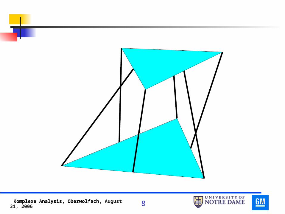
If the lengths of the six legs are fixed the platform robot is usually rigid.

Husty and Karger made a study of exceptional lengths when the robot will move: one interesting case is when the top joints and the bottom joints are in a configuration of equilateral triangles.


Another Example


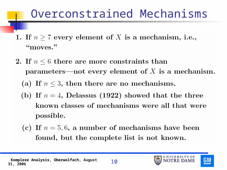
Overconstrained Mechanisms


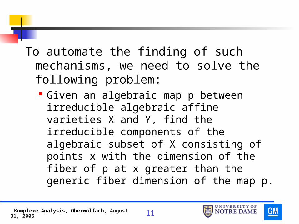
To automate the finding of such mechanisms, we need to solve the following problem: Given an algebraic map p between irreducible

algebraic affine varieties X and Y, find the irreducible components of the algebraic subset of X consisting of points x with the dimension of the fiber of p at x greater than the generic fiber dimension of the map p.


One Approach

A method to find the exceptional sets A.J. Sommese and C.W. Wampler, Exceptional

sets and fiber products, preprint.

A method to solve large systems with few solutions A.J. Sommese, J. Verschelde and C.W.

Wampler, Solving polynomial systems equation by equation, preprint.


Exceptional Sets


A Simple Example


Setup


Problem Statement


For

0);(212

11

xxq

xqqxf


Fiber Products


Main Components


The Notion of a Main Component


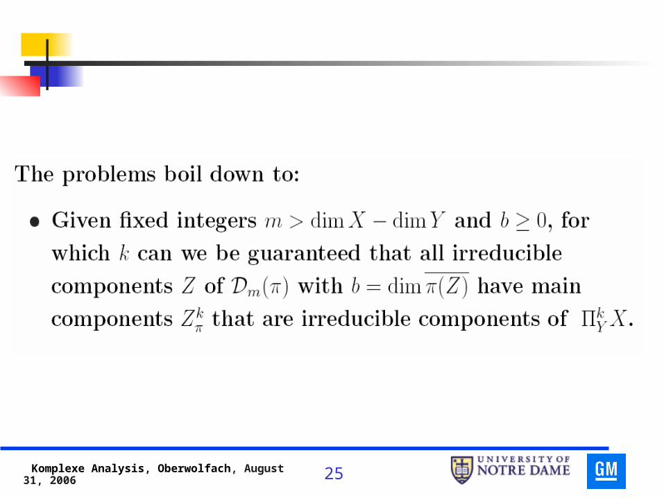
It is easy to recognize main components. An irreducible subset W of is a main component if

XkY

kZ


A Bound


An Alternate Bound


Numerical Algebraic Geometry

Isolated Solutions Positive Dimensional Solutions Bertini A Case Study


Computing Isolated Solutions

Find all isolated solutions in of a system on n polynomials:

NC

0

),...,(f

),...,(f

1n

11

N

N

xx

xx


Solving a system

Homotopy continuation is our main tool: Start with known solutions of a known start

system and then track those solutions as we deform the start system into the system that we wish to solve.


Path Tracking

This method takes a system g(x) = 0, whose solutions

we know, and makes use of a homotopy, e.g.,

Hopefully, H(x,t) defines “paths” x(t) as t runs

from 1 to 0. They start at known solutions of

g(x) = 0 and end at the solutions of f(x) at t = 0.

tg(x). t)f(x)-(1 t)H(x,


The paths satisfy the Davidenko equation

To compute the paths: use ODE methods to predict and Newton’s method to correct.

t

H

dt

dx

x

H

dt

t)dH(x(t),0

N

1

i

i

i


Solutions of

f(x)=0

Known solutions of g(x)=0

t=0 t=1H(x,t) = (1-t) f(x) + t g(x)

x3(t)

x1(t)

x2(t)

x4(t)


Newton correction

prediction

{

t

xj(t)

x*

01


Algorithms

middle 80’s: Projective space was beginning to be used, but the methods were a combination of differential topology and numerical analysis with homotopies tracked exclusively through real parameters.

early 90’s: algebraic geometric methods worked into the theory: great increase in security, efficiency, and speed.


Uses of algebraic geometry

Simple but extremely useful consequence of algebraicity [A. Morgan (GM R. & D.) and S.]

Instead of the homotopy H(x,t) = (1-t)f(x) + tg(x)

use H(x,t) = (1-t)f(x) + tg(x)


Genericity

Morgan + S. : if the parameter space is irreducible, solving the system at a random points simplifies subsequent solves: in practice speedups by factors of 100.


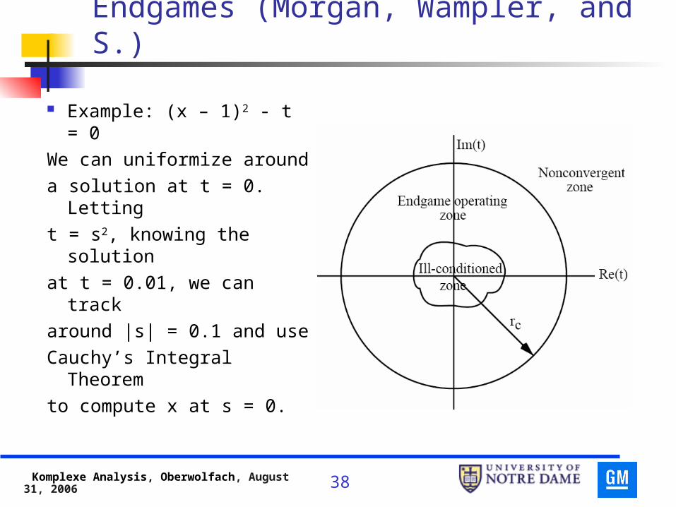
Endgames (Morgan, Wampler, and S.)

Example: (x – 1)2 - t = 0

We can uniformize around

a solution at t = 0. Letting

t = s2, knowing the solution

at t = 0.01, we can track

around |s| = 0.1 and use

Cauchy’s Integral Theorem

to compute x at s = 0.


Special Homotopies to take advantage of sparseness


Multiprecision

Not practical in the early 90’s! Highly nontrivial to design and dependent on

hardware Hardware too slow


Hardware

Continuation is computationally intensive. On average: in 1985: 3 minutes/path on largest mainframes.


Hardware

Continuation is computationally intensive. On average: in 1985: 3 minutes/path on largest mainframes. in 1991: over 8 seconds/path, on an IBM 3081;

2.5 seconds/path on a top-of-the-line IBM 3090.


Hardware

Continuation is computationally intensive. On average: in 1985: 3 minutes/path on largest mainframes. in 1991: over 8 seconds/path, on an IBM 3081;

2.5 seconds/path on a top-of-the-line IBM 3090. 2006: about 10 paths a second on an single

processor desktop CPU; 1000’s of paths/second on moderately sized clusters.


A Guiding Principle then and now

Algorithms must be structured – when possible – to avoid paths leading to singular solutions: find a way to never follow the paths in the first place.


Continuation’s Core Computation

Given a system f(x) = 0 of n polynomials in n unknowns, continuation computes a finite set S of solutions such that: any isolated root of f(x) = 0 is contained in S; any isolated root “occurs” a number of times

equal to its multiplicity as a solution of f(x) = 0; S is often larger than the set of isolated

solutions.


References

A.J. Sommese and C.W. Wampler, Numerical solution of systems of polynomials arising in engineering and science, (2005), World Scientific Press.

T.Y. Li, Numerical solution of polynomial systems by homotopy continuation methods, in Handbook of Numerical Analysis, Volume XI, 209-304, North-Holland, 2003.


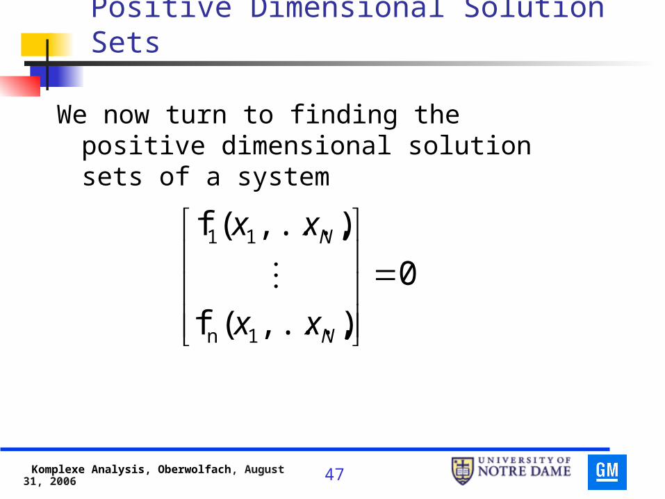
Positive Dimensional Solution Sets

We now turn to finding the positive dimensional solution sets of a system

0

),...,(f

),...,(f

1n

11

N

N

xx

xx


How to represent positive dimensional components?

S. + Wampler in ’95: Use the intersection of a component with

generic linear space of complementary dimension.

By using continuation and deforming the linear space, as many points as are desired can be chosen on a component.


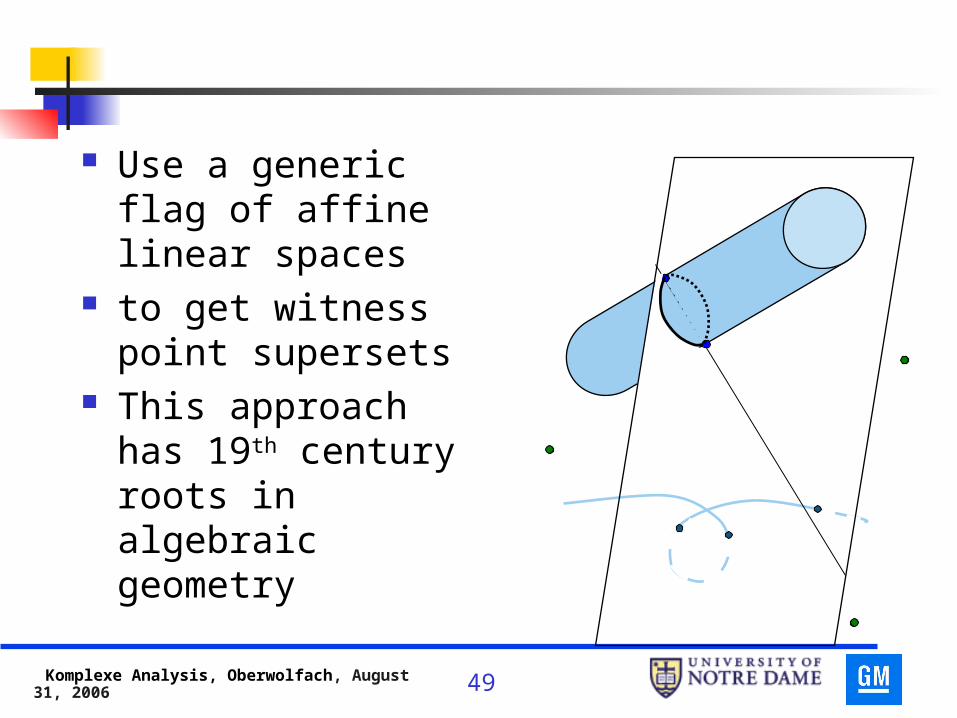
Use a generic flag of affine linear spaces

to get witness point supersets

This approach has 19th century roots in algebraic geometry


The Numerical Irreducible Decomposition

Carried out in a sequence of articles with

Jan Verschelde (Univiversity at Illinois at Chicago)

and Charles Wampler (General Motors Research and

Development) Efficient Computation of “Witness Supersets’’

S. and V., Journal of Complexity 16 (2000), 572-602. Numerical Irreducible Decomposition

S., V., and W., SIAM Journal on Numerical Analysis, 38 (2001), 2022-2046.


An efficient algorithm using monodromy S., V., and W., SIAM Journal on Numerical Analysis 40

(2002), 2026-2046.

Intersections of algebraic sets S., V., and W., SIAM Journal on Numerical Analysis 42

(2004), 1552-1571.


Symbolic Approach with same classical roots

Two articles in this direction: M. Giusti and J. Heintz, Symposia Mathematica

XXXIV, pages 216-256. Cambridge UP, 1993. G. Lecerf, Journal of Complexity 19 (2003), 564-596.


The Irreducible Decomposition


Witness Point Sets


Basic Steps in the Algorithm


Example


From Sommese, Verschelde, and Wampler,SIAM J. Num. Analysis, 38 (2001), 2022-2046.


Numerical issues posed by multiple components

Consider a toy homotopy

Continuation is a problem because the Jacobian with

respect to the x variables is singular.

How do we deal with this?

0),,(2

21

21

tx

xtxxH


Deflation

The basic idea introduced by Ojika in 1983 is

to differentiate the multiplicity away. Leykin,

Verschelde, and Zhao gave an algorithm for an

isolated point that they showed terminated.

Given a system f, replace it with

0

bzA

zJf(x)

f(x)


Bates, Hauenstein, Sommese, and Wampler:

To make a viable algorithm for multiple components, it is necessary to make decisions on ranks of singular matrices. To do this reliably, endgames are needed.


Bertini and the need for adaptive precision

Why use Multiprecision? to ensure that the region where an endgame

works is not contained the region where the numerics break down;





to ensure that a polynomial is zero at a point is the same as the polynomial numerically being approximately zero at the point;





to ensure that a polynomial is zero at a point is the same as the polynomial numerically being approximately zero at the point;

to prevent the linear algebra in continuation from falling apart.


Evaluation

To 15 digits of accuracy one of the roots of this polynomial is a = 27.9999999999999. Evaluating p(a) to 15 digits, we find that

p(a) = -2. Even with 17 digit accuracy, the approximate root a

is a = 27.999999999999905 and we still only have p(a) = -0.01.

128)( 910 zzzp


Wilkinson’s Theorem Numerical Linear Algebra

Solving Ax = f, with A an N by N matrix,

we must expect to lose digits of

accuracy. Geometrically, is

on the order of the inverse of the distance in

from A to to the set defined by det(A) = 0.

)](cond[log10 A

||||||||)( cond 1 AAA1NNP


One approach is to simply run paths that fail over at a higher precision, e.g., this is an option in Jan Verschelde’s code, PHC.


One approach is to simply run paths that fail over at a higher precision, e.g., this is an option in Jan Verschelde’s code, PHC.

Bertini is designed to dynamically adjust the precision to achieve a solution with a prespecified error. Bertini is being developed by Daniel Bates, Jon Hauenstein, Charles Wampler, and myself (with some early work by Chris Monico).


Issues

You need to stay on the parameter space where your problem is: this means you must adjust the coefficients of your equations dynamically.


Issues

You need to stay on the parameter space where your problem is: this means you must adjust the coefficients of your equations dynamically.

You need rules to decide when to change precision and by how much to change it.


The theory we use is presented in the article D. Bates, A.J. Sommese, and C.W. Wampler,

Multiprecision path tracking, preprint.

available at www.nd.edu/~sommese


Case Study: Alt’s Problem

We follow


A four-bar planar linkage is a planar quadrilateral with a rotational joint at each vertex.

They are useful for converting one type of motion to another.

They occur everywhere.


How Do Mechanical Engineers Find Mechanisms?

Pick a few points in the plane (called precision points)

Find a coupler curve going through those points

If unsuitable, start over.


Having more choices makes the process faster.

By counting constants, there will be no coupler curves going through more than nine points.


Nine Point Path-Synthesis Problem

H. Alt, Zeitschrift für angewandte Mathematik und Mechanik, 1923:

Given nine points in the plane, find the set of all four-bar linkages, whose coupler curves pass through all these points.


First major attack in 1963 by Freudenstein and Roth.


D′

Pj

δj

λj

µj

u b v

CD

x

y

P0

C′


Pj

δj

µj

b-δj

v

C

y

P0

θj

yeiθj

b

v = y – b

veiμj = yeiθj - (b - δj)

= yeiθj + δj - b

C′


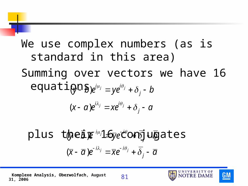
We use complex numbers (as is standard in this area)

Summing over vectors we have 16 equations

plus their 16 conjugates

byeeby jii jj )(

axeeax jii jj )(

beyeby jii jj )(

aexeax jii jj )(


This gives 8 sets of 4 equations:

in the variables a, b, x, y, and

for j from 1 to 8.

byeeby jii jj )(

axeeax jii jj )(

beyeby jii jj )(

aexeax jii jj )(

,y ,x ,b ,a

jjj ,,λ


Multiplying each side by its complex conjugate

and letting we get 8 sets of 3 equations

in the 24 variables

with j from 1 to 8.

0δδ - x)- a(δ )x - a(δγ x)δ - (a γ)xδ - a( jjjjjjjj

0δδ - y) - b(δ )y - b(δγ y)δ - (b γ)yδ - b( jjjjjjjj

0γγγγ jjjj

jj γ, γand y ,x ,b ,a y, x,b, a,

1eγ jiθj


in the 24 variables

with j from 1 to 8.

0δδ - x) -a (δ )x - a(δγ x)δ -(a γ)xδ - a( jjjjjjjj

0δδ - y)- b(δ )y - b(δγ y)δ - (b γ)yδ - b( jjjjjjjj

0γγγγ jjjj

jj γ, γand y ,x ,b ,a y, x,b, a,


Using Cramer’s rule and substitution we have

what is essentially the Freudenstein-Roth

system consisting of 8 equations of degree 7.

Impractical to solve: 78 = 5,764,801solutions.


Newton’s method doesn’t find many solutions: Freudenstein and Roth used a simple form of continuation combined with heuristics.

Tsai and Lu using methods introduced by Li, Sauer, and Yorke found only a small fraction of the solutions. That method requires starting from scratch each time the problem is solved for different parameter values


Solve by Continuation

All 2-homog.systems

All 9-pointsystems

“numerical reduction” to test case (done 1 time)

synthesis program (many times)

komplexe analysis, oberwolfach, august 31, 2006 exceptional sets and fiber products andrew sommese...

Documents